uncertainty-driven business cycles: assessing the markup
TRANSCRIPT

Uncertainty-driven business cycles:assessing the markup channel�
Benjamin Born Johannes Pfeifer
September 8, 2020
Abstract
Precautionary pricing and increasing markups in representative-agent DSGE modelswith nominal rigidities are commonly used to generate negative output e�ects ofuncertainty shocks. We assess whether this theoretical model channel is consistent withthe data. Three things stand out. First, consistent with precautionary wage setting,we find that wage markups increase after uncertainty shocks. Second, the impulseresponses of price markups are largely inconsistent with the standard model, both at theaggregate as well as the industry level. Finally, and in contrast to times-series evidence,our theoretical model robustly predicts that uncertainty shocks have a quantitativelysmall impact on the economy.
Keywords: Uncertainty shocks, precautionary pricing, markup channel,price markup, wage markup
JEL-Codes: E32, E01, E24
�Born: Frankfurt School of Finance & Management, CEPR, and CESifo, [email protected], Pfeifer: BundeswehrUniversity Munich, [email protected]. We would like to thank the editor, Kjetil Storesletten, andthree anonymous referees, as well as Angela Abbate, Klaus Adam, Lukas Freund, Matthias Hartmann,Alex Kriwoluzky, Keith Kuester, Ariel Mecikovsky, Gernot Müller, Morten Ravn, Mirko Wiederholt, andaudiences at the Universities of Aarhus, Barcelona, Frankfurt, Göttingen, Halle, Heidelberg, Cologne,Lüneburg, Southampton, Toulouse, and Tübingen, as well as at University College London, the CESifo SurveyConference 2016, the CIRET/KOF/RIED WSE Workshop 2015, the Dynare Conference 2016, the ECB,ESSIM 2016, the Frankfurt-Mannheim Workshop 2015, the EU Joint Research Council at Ispra, T2M 2016,the Annual Meeting of the Verein für Socialpolitik 2016, and the Meeting of the Macroeconomic Council ofthe Verein für Socialpolitik 2017 for helpful comments and suggestions. Special thanks go to Randy A. Beckerand Wayne Gray for important clarifications regarding the NBER-CES Manufacturing Industry Database.
1 IntroductionSince the seminal paper by Bloom (2009), many studies have focused on the e�ects ofuncertainty shocks on economic fluctuations (see Castelnuovo 2019, for a survey). Whiletime-series approaches regularly find negative e�ects of uncertainty shocks on output (Baker,Bloom, and Davis 2016; Jurado, Ludvigson, and Ng 2015; Bachmann, Elstner, and Sims2013, and numerous others),1 it has proven surprisingly di�cult to generate negative outpute�ects after uncertainty shocks in representative-agent models as uncertainty shocks areexpansionary in the standard RBC model.2 As shown by Fernández-Villaverde, Guerrón-Quintana, Kuester, and Rubio-Ramírez (2015), Born and Pfeifer (2014a), and Basu andBundick (2017) and used in various papers, countercyclical aggregate markups of the formpresent in standard New Keynesian (NK) models are key to match the empirical evidence.Many recent representative-agent DSGE studies rely on this countercyclical movement ofprice and/or wage markups conditional on uncertainty shocks.3 However, direct empiricalevidence on the presence of this transmission channel is limited.
We therefore assess whether this so-called “markup channel” is consistent with the data.To this end, we build and (partially) estimate an NK DSGE model with time-varying priceand wage markups that serves two purposes. First, the dynamic dimension of the model isused to generate predictions on the e�ects of uncertainty shocks on price and wage markupsthat can be empirically tested. Second, the intratemporal first-order conditions can be usedas a Chari, Kehoe, and McGrattan (2007)-type business cycle accounting framework toconstruct aggregate price and wage markups from the data.
As predicted by the previous literature, in the model an increase in uncertainty leadsto an increase in both price and wage markups and a decline in output, whereas withoutnominal rigidities the precautionary labor supply motive dominates and output increases.However, overall, the model-implied e�ects of uncertainty shocks on output are quantitativelysmall. This is due to two things. First, we employ a micro-estimate-based, conservativemodel parameterization not specifically tailored to generate large e�ects. Second and mostimportantly, our driving processes estimated using full information techniques do not featurelarge and persistent increases in uncertainty.
1See Berger, Dew-Becker, and Giglio (2020) for a countervailing viewpoint that it is only realized volatilityand not future uncertainty that matters.
2The present paper is not concerned with heterogeneous agent models with non-convex adjustment costsand idiosyncratic uncertainty like Bloom (2009) and Bachmann and Bayer (2013), where real options e�ectsare responsible for the negative e�ects of uncertainty.
3E.g. Ba�kaya, Hülagü, and Kü�ük (2013), Mumtaz and Zanetti (2013), Cesa-Bianchi and Fernandez-Corugedo (2018), Carriero, Mumtaz, Theodoridis, and Theophilopoulou (2015), Alessandri and Mumtaz(2019), Castelnuovo and Pellegrino (2018), and Leduc and Liu (2016). Notable exceptions are Christiano,Motto, and Rostagno (2014) and Chugh (2016), who embed uncertainty in a financial accelerator mechanism.
1
Time-series techniques are then used to identify uncertainty shocks in the data and tostudy whether the conditional comovement between markups and output is consistent withthe one implied by the model. Overall, we find that in the data, wage markups consistentlyincrease after identified uncertainty shocks as the model predicts. This finding is robust acrossdi�erent identification schemes as well as uncertainty and wage markup measures. In contrast,the impulse responses of price markups are largely inconsistent with the standard model. Wedo not find robust evidence for a strong increase in price markups, neither at the aggregatenor at the industry level, regardless of whether markups are measured along the intensivelabor or the intermediate input margin. The only exception is the extensive labor margin,where price markups tend to increase. This latter finding suggests that recent modeling e�ortscombining search-and-matching models with uncertainty shocks are particularly promisingfor obtaining data-consistent responses (Leduc and Liu 2016; den Haan, Freund, and Rendahl2020).
Our findings come with obvious caveats. There is no consensus on how to measuremarkups, neither at the aggregate nor the individual level.4 The same applies to measuringuncertainty and identifying uncertainty shocks. To alleviate these concerns, we show thatour results are robust to employing various uncertainty measures, identification schemes,and assumptions for measuring markups. Nevertheless, results will always rely on modelingassumptions. Despite this drawback, we consider theory-driven studies of markups useful asthey may inform us on both the likely validity of the underlying model’s assumptions andthe measurement approach itself.
Our investigation of price markups is most closely related to Nekarda and Ramey (2013),who argue that aggregate price markups are pro- to acyclical unconditionally and alsoregularly do not show the conditional movement after shocks predicted by standard NKmodels. However, they do not consider uncertainty shocks and only focus on the pricemarkup, while the main e�ect might work through wage markups. This is important as,e.g., Karabarbounis (2014) argues that about 90% of the cyclical movement in the totalmarkup derives from movements in the wage component of this markup. Fernández-Villaverdeet al. (2015) provide some tentative evidence of an increase in the price markup following anuncertainty shock. But this critically relies on estimating uncertainty shocks based on anexogenous process, but subsequently treating these exogenous shocks as endogenous variablesin an unrestricted VAR. Recently, Basu and House (2016) and Bils, Klenow, and Malin (2018)(BKM in the following) have argued that measured average hourly earnings often are notallocative due to the presence of implicit contracts and composition e�ects and, as BKM
4See e.g. the discussions in Nekarda and Ramey (2013), Anderson, Rebelo, and Wong (2018), and DeLoecker, Eeckhout, and Unger (2020).
2
argue, this distorts the cyclicality of the resulting price markups. BKM, therefore, propose torather measure price markups for the self-employed and along the intermediate input margin.Our paper is also related to earlier papers studying the (unconditional) cyclical movementof (price) markups, surveyed in Rotemberg and Woodford (1999), as well as “business cycleaccounting” studies like Chari et al. (2007) and Hall (1997). Galí, Gertler, and López-Salido(2007) is an influential study that decomposes the labor wedge into a firm and a householdcomponent to study the welfare implications of labor-wedge fluctuations.
Section 2 provides a detailed exposition on the mechanism embedded in NK models thatgives rise to contractionary uncertainty e�ects. Section 3 presents a baseline NK DSGE withtime-varying wage and price markups and documents the predicted conditional comovementof output and markups following uncertainty shocks. The intratemporal first-order conditionsof the model also provide an accounting framework, which is used to construct markups fromthe data. Section 4 then identifies uncertainty shocks from the data, studies whether theconditional comovement between markups and output is consistent with the one implied bythe model, and provides robustness checks. Section 5 investigates the price markup responseat the industry level. Section 6 concludes.
2 Precautionary pricing: a stylized modelAs shown by Basu and Bundick (2017), the reason that uncertainty is expansionary in thestandard RBC model is the presence of a “precautionary labor supply” motive. When facedby higher uncertainty, the household does not only self-insure by consuming less and investingmore, but also by working more. From the neoclassical production function, where TFPis una�ected by uncertainty and capital is predetermined, it follows that this increase inlabor results in an output expansion that fuels higher savings. The solution to generatecontractionary e�ects of uncertainty is to break this tight link between labor supply andproduction. This can be achieved by introducing monopolistic competition in labor and goodsmarkets, which gives rise to time-varying markups (see also Fernández-Villaverde et al. 2015;Born and Pfeifer 2014a). In the presence of sticky prices and wages, firms and households intheir price- and wage-setting decisions face a convex marginal revenue product. This gives riseto inverse Oi-Hartman-Abel-e�ects and precautionary pricing when faced with uncertaintyabout future economic variables. Price-setters face the following choice: If prices are set toolow, more units need to be sold at too low a price, which is bad for the firm. In contrast, ifprices are set too high, the higher price compensates for being able to sell fewer units. Dueto this asymmetric, nonlinear e�ect, price setters prefer to err on the side of too high pricesand increase their markups. It is instructive to consider the case of perfect competition. If
3
0.95 1 1.05 1.1
≠0.02
0.01
0.04
0.07
0.10
pi,t≠1
Period Profit
0.95 1 1.05 1.1
≠0.02
0.01
0.04
0.07
0.10
pi,t≠1
Expected Profit
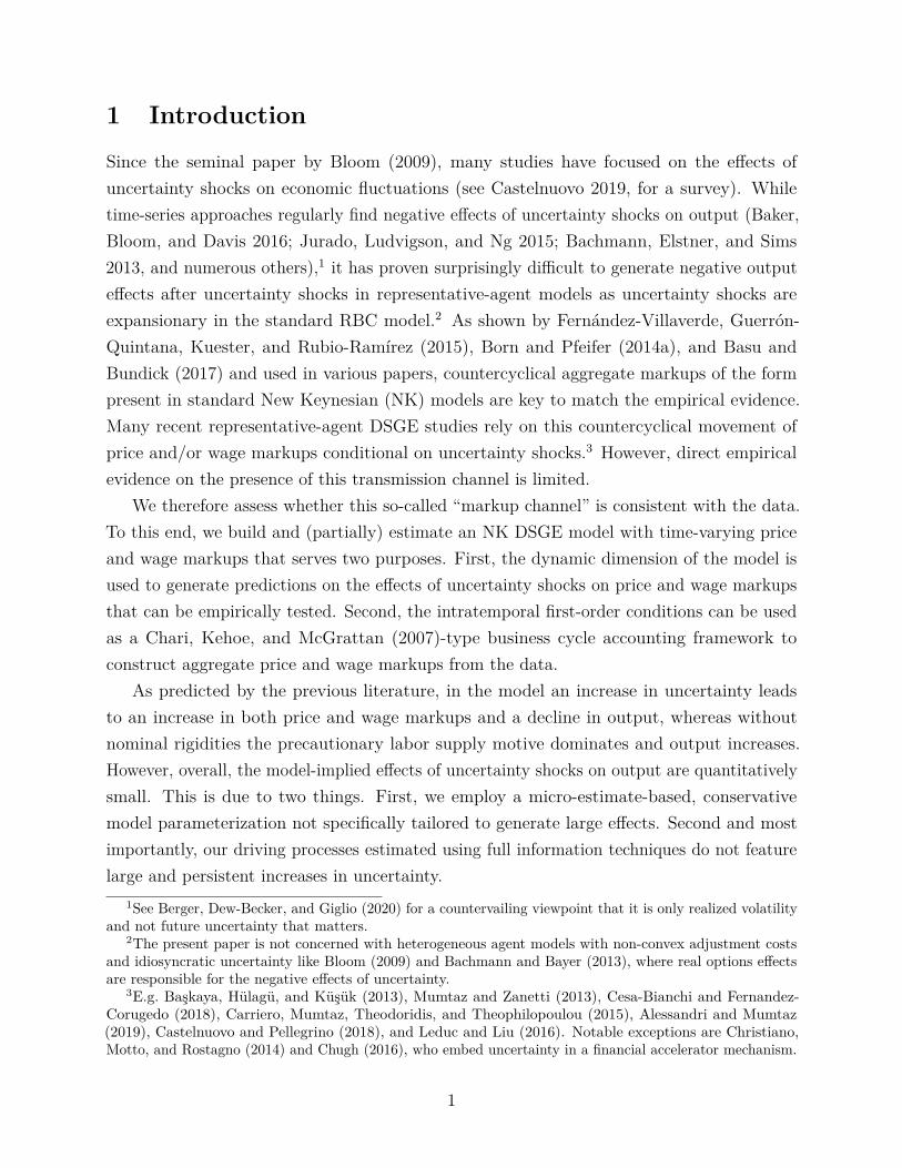
Figure 1: Stylized pricing example. Notes: period profit (left panel) and expected profit ofthe firm (right panel) as function of the price pi,t≠1. The black dashed line indicatesthe maximum of the respective function. Red dashed line: mean preserving spreadto the optimal price that the firm faces. Blue dash-dotted line: profits whenchoosing the mean optimal price of 1.
the price is just an epsilon below marginal costs, the firm will have to satisfy all demand at aloss, leading to (potentially) unbounded losses. In contrast, if the price is just an epsilon toohigh, the firm will face zero demand. Hence, the worst case if the price is too high is zeroprofits. If this increase in markups after uncertainty shocks is strong enough, it dampensdemand and decreases output.
To see this more clearly, consider the following stylized partial equilibrium example. Afirm i of a continuum of identical, monopolistically competitive firms chooses its optimalprice pi,t≠1 subject to a Dixit-Stiglitz-type demand function yi,t =
1pi,t≠1
pt
2≠◊pyt, where yt
is aggregate demand, ◊p is the demand elasticity, and pt the aggregate price level. For themechanism to be as transparent as possible, we assume the firm is subject to a Taylor-typepricing friction in that it has to set its price one period in advance.5 Its output is producedusing a constant returns to scale production function that is linear in labor: yi,t = li,t. Thelabor market is assumed to be competitive, with the economy-wide wage being denoted bywt. Real firm profits are then given by
fi =C
pi,t≠1pt
≠ wt
pt
D Api,t≠1
pt
B≠◊p
yt . (2.1)
5A similar mechanism is also present in the Rotemberg price adjustment cost framework used in themedium-scale NK model below as well as in Calvo- and Menu Cost-models. In these settings, marginal profitsare still convex in the price (see, e.g., Fernández-Villaverde et al. 2015; Balleer, Hristov, and Menno 2017).While the logic in a symmetric Rotemberg equilibrium is a bit more involved (see Oh forthcoming), theunderlying upward pressure on markups resulting from the nonlinear Phillips Curve is still crucial.
4

Without loss of generality, assuming for the aggregate variables that yt = 1 and wtpt
=(◊p ≠ 1)/◊p, this simplifies to
fi =C
pi,t≠1pt
≠ ◊p ≠ 1◊p
D Api,t≠1
pt
B≠◊p
. (2.2)
Expression (2.2) shows that there are two di�erent channels through which prices a�ectprofits. First, a higher price pi,t≠1 has an immediate price impact on the revenue, while leavingthe marginal costs una�ected. But second, there is an additional impact on the quantitysold. The left panel of Figure 1 shows the profit function for ◊p = 11. As is well-known, inthe absence of uncertainty the firm will optimally charge a gross markup ◊p
◊p≠1 over marginalcosts, resulting in a profit-maximizing price of pi,t≠1 = 1.
Assume now that the firm faces uncertainty about the optimal price, because the aggregateprice level is with probability 1/2 either pt = 1/1.05 or pt = 1/0.95, so that in the absence ofpricing frictions, either pi,t = 0.95 or pi,t = 1.05 is optimal. Thus, compared to the previoussituation, the optimal price is subject to a mean-preserving spread.6 Setting the price at theexpected optimal pi,t≠1 = 1 is suboptimal, because it would lead to lower expected profitsdue to the marginal profit being convex in the price. Rather, the optimal price in this case isslightly higher at pi,t≠1 = 1.02. This can be seen in the expected profit schedule as a functionof pi,t≠1 shown in the right panel of Figure 1. A formal proof can be found in Appendix E.
The same mechanism is at work in the household sector where the households have tomaximize utility by setting a nominal wage subject to an equivalent demand function fortheir labor services.7
We close this section by pointing out that the empirical test of the markup channel hasimplications beyond the precautionary pricing mechanism outlined above. Even in modelswhere precautionary pricing is shut o� by linearizing the New Keynesian Phillips Curves,countercyclical markups due to nominal rigidities are key because they are instrumental inamplifying “run-of-the-mill” demand e�ects (see the excellent discussion in den Haan et al.2020). A case in point is the work of Leduc and Liu (2016), whose search-and-matchingframework generates negative output e�ects even in a flex-price model via nonlinearities in
6For ease of exposition we consider a mean-preserving spread to the endogenous variable. The same e�ectwould arise following a mean-preserving spread to aggregate price pt, but in this case an additional Jensen’sInequality e�ect would complicate matters due to the price level entering in the denominator.
7The asymmetry of the profit function comes from the isoelastic Dixit-Stiglitz demand function paired withthe assumption that demand always has to be satisfied. For small to moderate shocks, the latter assumptioncan be justified by contractual obligations and reputational concerns. Firms tend to not close shop if theirposted price turns out to be too low, while workers cannot stay at home when asked to work overtime, evenif their marginal rate of substitution turns out to be high. However, these considerations also suggest thatfirms can more easily avoid having to satisfy demand by “being out of stock”. This potential violation of acrucial model assumption may be one reason why we find less evidence of a precautionary pricing for firms.
5

the wage setting equation. However, even in their setting, price rigidities and the associatedcountercyclical price markup are used in the final model to provide key amplification (up toa factor of 20).
3 ModelIn this section we construct a prototypical New Keynesian DSGE model that embeds thepreviously outlined mechanism on the firm and household side. The model serves twopurposes. First, the dynamic dimension of the model can be used to generate predictionson the e�ects of uncertainty shocks on price and wage markups. Second, the intratemporalfirst-order conditions can be used as a Chari et al. (2007)-type business cycle accountingframework to construct aggregate price and wage markups from the data.
The model economy is populated by a continuum of intermediate good firms producingdi�erentiated intermediate goods using bundled labor services and capital, and a final goodfirm bundling intermediate goods to a final good. A continuum of households j œ [0, 1] sellsdi�erentiated labor services to a labor bundler. In addition, the model features a governmentsector that finances government spending with distortionary taxation and transfers, and amonetary authority, which sets the nominal interest rate according to an interest rate rule.The full set of model equations is relegated to Appendix A.1.
3.1 Firms
The final good Yt is assembled from a continuum of di�erentiated intermediate inputs Yt(i),i œ [0, 1], using the constant returns to scale Dixit-Stiglitz-technology
Yt =5⁄ 1
0Yt(i)
◊p≠1◊p di
6 ◊p◊p≠1
, (3.1)
where ◊p > 0 is the elasticity of substitution between intermediate goods. Standard costminimization yields the demand for good i:
Yt(i) =C
Pt(i)Pt
D≠◊p
Yt , (3.2)
where Pt is the aggregate price level.The monopolistically competitive intermediate good firms produce Yt(i) using capital
6

Kt(i) and a hired composite labor bundle Nt(i) according to a CES production function
Yt(i) = Ynorm
Y]
[–
5Kt (i)
6 Â≠1Â
+ (1 ≠ –)5Zt (Nt (i) ≠ N
o)6 Â≠1
Â
Z^
\
ÂÂ≠1
≠ � .
Here, 0 Æ – Æ 1 parameterizes the labor share and Ynorm is a normalization factor that
makes output equal to one in steady state. is the elasticity of substitution between capitaland labor, with  = 1 being the Cobb-Douglas case. The fixed cost of production � reduceseconomic profits to zero in steady state, thereby ruling out entry or exit (see, e.g., Christiano,Eichenbaum, and Evans 2005). N
o = „oN , where N denotes steady-state labor, is overheadlabor used in the production of goods.8 Zt denotes a stationary, labor-augmenting technologyprocess specified below. Each intermediate good firm owns its capital stock, whose law ofmotion is given by
Kt+1(i) = (1 ≠ ”) Kt(i) +Q
a1 ≠ „K
2
AIt(i)
It≠1(i)≠ 1
B2R
b It(i) , „K Ø 0 , (3.3)
where ” denotes the quarterly depreciation rate of the capital stock. Equation (3.3) includesinvestment adjustment costs at the firm level of the form popularized by Christiano et al.(2005).
Intermediate good producers are owned by households and therefore use the households’stochastic discount factor for discounting. They maximize the present discounted value ofper period profits subject to the law of motion for capital and the demand from the finalgood producer:
CPt(i)Pt
D1≠◊p
Yt ≠ Wt
Pt
Nt(i) ≠ It(i) ≠ „p
2
APt(i)
Pt≠1(i)≠ �
B2
Yt(i) , (3.4)
where Nt(i) is hired in a competitive rental market at given wage rate Wt. The last termdenotes Rotemberg price adjustment costs as in Fernández-Villaverde et al. (2015), where �is steady-state inflation. From the firms’ cost minimization problem follows the first-ordercondition for labor inputs as
�p,t
Wt
Pt
= MPLt , (3.5)
where �p,t is the gross price markup over marginal costs. Due to monopolistic competition,�p,t will generally not be equal to 1 as firms set a markup over marginal costs. Time-variation
8Overhead labor, apart from being an empirically realistic feature, allows the marginal wage in the economyto di�er from the average wage. This is important, because it makes the price markup more countercyclicalthan would be inferred from the rather a-cyclical total labor share alone (see, e.g., Rotemberg and Woodford1999).
7

in this markup is a central element of shock transmission in the NK model.
3.2 Households
Following Erceg, Henderson, and Levin (2000), we assume that the economy is populatedby a continuum of monopolistically competitive households, supplying di�erentiated laborNt(j) at wage Wt(j) to a labor bundler who then supplies the composite labor input to theintermediate good producers. Formally, the aggregation technology follows a Dixit-Stiglitzform
Nt =5⁄ 1
0Nt(j)
◊w≠1◊w dj
6 ◊w◊w≠1
, ◊w > 0 . (3.6)
Expenditure minimization yields the optimal demand for household j’s labor as
Nt(j) =C
Wt(j)Wt
D≠◊w
Nt ’ j . (3.7)
Household j has preferences
Vt =Œÿ
h=0—
h[(Ct+h(j))÷(1 ≠ Nt+h(j))1≠÷]1≠‡ ≠ 1
1 ≠ ‡, (3.8)
where the parameter ‡ Ø 0 measures the risk aversion, 0 < — < 1 is the discount rate,and 0 < ÷ < 1 denotes the share of the consumption good in the consumption-leisureCobb-Douglas bundle.
The household faces the budget constraint
(1 + ·c
t)Ct(j) + Bt(j)
Pt
Æ(1 ≠ ·n
t)Wt(j)
Pt
Nt(j) + Rt≠1Bt≠1(j)
Pt
+ Dt(j)
≠ „w
2
A
�≠1 Wt(j)Wt≠1(j) ≠ 1
B2
Yt + Tt ,
(3.9)
where the household earns income from supplying di�erentiated labor, which is taxed atrate ·
n
t. In addition, it receives real dividends Dt(j) from owning a share of the firms in the
economy and a real gross return Rt≠1(Bt≠1(j)/Pt) from investing in a zero net supply risklessnominal bond. The household spends its income on consumption Ct(j), taxed at rate ·
c
t, real
savings in the private bond Bt(j)/Pt, and to cover the costs of adjusting its wage (the secondto last term on the right hand side). Finally, Tt denotes transfers/lump-sum taxes.
The optimization problem of the household involves maximizing (3.8) subject to thebudget constraint (3.9) and the demand for the household’s di�erentiated labor input (3.7).The first-order condition for labor supply implies that a gross markup over the after-tax
8

marginal rate of substitution �w,t is chosen such that
Wt
Pt
= �w,t
1 + ·c
t
1 ≠ ·nt
(≠1)VN,t
VC,t
,
where VN and VC are the partial derivatives of the utility function with respect to labor andconsumption, respectively.
3.3 Government Sector
The government’s budget constraint is given by
·c
tCt + ·
n
t
Wt
Pt
Nt = Gt + Tt , (3.10)
where Gt is exogenous government consumption and where we have suppressed aggregationover households j for notational convenience.
The model is closed by assuming that the central bank follows a Taylor rule that reactsto inflation and output:
Rt
R=
3Rt≠1
R
4flR
Q
aA
�t
�
B„Rfi
AYt
Y HPt
B„Ry
R
b1≠flR
. (3.11)
Here, 0 Æ flR Æ 1 is a smoothing parameter introduced to capture the empirical evidence ofgradual movements in interest rates, � is the target inflation rate set by the central bank,and the parameters „Rfi and „Ry capture the responsiveness of the nominal interest rateto deviations of inflation from its steady-state value and output from its model-consistentHodrick and Prescott (HP) filter trend Y
HP
t, respectively.9
3.4 Exogenous shock processes
The two exogenous processes for government spending and TFP follow AR(1)-processes withstochastic volatility:
Zt = flzZt≠1 + ‡z
tÁ
z
t(3.12)
Gt = flgGt≠1 + „gyYt≠1 + ‡g
t Ág
t (3.13)
‡z
t= (1 ≠ fl‡z)‡z + fl‡z‡
z
t≠1 + ÷‡zÁ‡
z
t(3.14)
‡g
t = (1 ≠ fl‡g)‡g + fl‡g‡g
t≠1 + ÷‡gÁ‡
g
t, (3.15)
9This specification follows Born and Pfeifer (2014a). The HP filtered output gap is embedded into thedynamic rational expectations model following the approach of Cúrdia, Ferrero, Ng, and Tambalotti (2015).
9

where the Ái
t, i œ {z, g, ‡
z, ‡
g} are standard normally distributed i.i.d. shock processes, hatsdenote percentage deviations from trend, and „gy governs the output feedback to governmentspending. ‡
z
tand ‡
g
t are our proxies for supply and demand uncertainty, respectively, withÁ
‡z
tand Á
‡z
tbeing the corresponding uncertainty shocks.
3.5 Equilibrium
The use of Rotemberg price and wage adjustment costs implies the existence of a representativefirm and a representative household. We consider a symmetric equilibrium in which allintermediate good firms charge the same price and choose the same labor input and capitalstock. Similarly, all households set the same wage, supply the same amount of labor, andwill choose the same consumption and savings.
The resource constraint then implies that output is used for consumption, investment,government spending, and to pay for price and wage adjustment costs:
Yt = Ct + It + Gt + „w
2
A
�≠1 Wt
Wt≠1≠ 1
B2
Yt + „p
2
A
�≠1 Pt
Pt≠1≠ 1
B2
Yt . (3.16)
3.6 Parametrization
Table 1 displays the parametrization of our quarterly model for the US economy from 1964Q1to 2015Q4. The capital share – is set to one third and the depreciation rate ” to imply anannual depreciation rate of 10 percent. The discount factor — = 0.995 implies an annualizedinterest rate of 2% in steady state. The investment adjustment cost parameter „k is set to2.5, the value estimated in Christiano et al. (2005).
The price adjustment cost parameter „p is chosen to imply the same slope of the linearNew Keynesian Phillips Curve as a Calvo model with an average price duration of 3 quarters.While this value is in the range of typical estimates based on micro data (e.g. Nakamura andSteinsson 2008), it is slightly lower than the typical value of 4 quarters used in the uncertaintyliterature (e.g. Leduc and Liu 2016; Basu and Bundick 2017; Fernández-Villaverde et al.2015). Similarly, the wage adjustment cost parameter is chosen to imply an average wagecontract duration of 3 quarters (see Born and Pfeifer 2020). We will explore the robustnessto these choices below. The two substitution elasticity parameters ◊p and ◊w are set to 11,which implies a steady-state markup of 10%.
We consider a zero-inflation steady state, i.e. � = 1. The Taylor rule parameters arestandard values in the literature with a moderate degree of interest smoothing and outputfeedback.10 The risk aversion parameter is set to ‡ = 2. The leisure share in the Cobb-Douglas
10It should be noted that the choice of monetary policy is not completely innocuous. If the central bank
10

Table 1: Model Parametrization
Parameter Description Value Target– Capital share 0.094 Capital share of 1/3— Discount factor 0.995 2% annualized interest rate” Depreciation rate 0.025 10% per year‡ Risk aversion 2 standard value„k Inv. adj. costs 2.5 Christiano, Eichenbaum, and Evans (2005)„p Price adj. costs 59 Implied average duration of 3 quarters„w Wage adj. costs 371 Implied average duration of 3 quarters◊w Labor subst. ela. 11 10% steady-state markup◊p Goods subst. ela. 11 10% steady-state markup÷ Leisure share 0.468 Frisch elasticity of 1„
o Overh. lab. share 0.11 Nekarda and Ramey (2013)Â Subst. ela. CES 0.5 Chirinko (2008)� Fixed costs 0.019 0 Steady-state profits� Ss gross inflation 1 Zero inflationflr Interest smoothing 0.75 Standard value„Rfi Inflation feedback 1.35 Standard value„Ry Output feedback 0.125 Standard value·
c Cons. tax rate 0.094 Sample mean·
n Labor tax rate 0.220 Sample meanG/Y G/Y share 0.206 Sample meanY
norm Output normalization 1.351 Output of 1
utility bundle ÷ is set to imply a Frisch elasticity of 1.11 We set the share of overhead laborto 11%, following the evidence of Levitt, List, and Syverson (2013) that adding a second shiftin car manufacturing plants increases labor by 80%. Given that automobile plants run twoshifts most of the time, this means overhead labor accounts for 20/180 = 0.11 (see Nekardaand Ramey 2013). The fixed costs � are set to imply 0 profits in steady state, thereby rulingout entry and exit.12 The substitution elasticity between capital and labor is set to  = 0.5,the midpoint of the estimates surveyed in Chirinko (2008) and in line with Chirinko andMallick (2017) and Oberfield and Raval (2019).13 The fiscal parameters are set to their meanover the sample 1964Q1 to 2015Q4. The tax rates are computed as average e�ective tax rates
puts relatively little weight on current inflation, it will tolerate large deviations of sticky prices from theiroptimal target. Firms will anticipate this and react with strong precautionary pricing. For the parameterranges typically found in the literature, we experienced quantitative di�erences, but the qualitative e�ect weare investigating in this paper remained una�ected.
11See Appendix A.2.1.12Note that in contrast to e.g. Smets and Wouters (2007), these fixed costs are non-labor related fixed
costs as the latter are captured in the overhead labor share.13We verified that our results are robust to variations in the substitution elasticity; see Section 4.5 below.
11

following Jones (2002).14
Table 2: Prior and Posterior Distributions of the Shock Processes
Parameter Prior distribution Posterior distributionDistribution Mean Std. Dev. Mean 5 % 95 %
G processfl‡g Beta* 0.90 0.100 0.513 0.313 0.708flg Beta* 0.90 0.100 0.945 0.883 0.999÷‡g Gamma 0.50 0.100 0.003 0.002 0.004‡
g Uniform 0.05 0.014 0.008 0.007 0.009„gy Normal 0.00 1.000 0.028 -0.026 0.083
TFP processfl‡z Beta* 0.90 0.100 0.517 0.312 0.722flz Beta* 0.90 0.100 0.773 0.692 0.855÷‡z Gamma 0.50 0.100 0.002 0.002 0.003‡
z Uniform 0.05 0.014 0.007 0.006 0.008
Note: Beta* indicates that the parameter divided by 0.999 follows a betadistribution. The sample ranges from 1964Q1 to 2015Q4 (N=208).
Finally, the exogenous processes are estimated via Bayesian techniques using sequentialMonte Carlo Methods on a quarterly US sample from 1964Q1 to 2015Q4.15 To constructoutput, government spending, and TFP deviations from trend, a one-sided HP-filter (⁄ = 1600)is used. For TFP, we cumulate the utilization-adjusted TFP series constructed by Fernald(2012).16 Table 2 displays the prior and posterior distributions, while Figure A.1 shows thesmoothed volatilities.
3.7 Dynamic e�ects of uncertainty shocks
As outlined in Section 2, precautionary price and wage setting in response to an increase inuncertainty lead to an increase in both price and wage markups. Thinking about a stylizedlabor market as depicted in the schematic diagram shown in Figure 2, this should cause boththe labor demand and supply curves to shift to the left, resulting in an overall decrease inhours worked and a reduction in aggregate output.
We can now feed uncertainty shocks into our general-equilibrium model to study the14While we allow tax rates to vary in the empirical analysis, we keep them fixed at their steady-state value
for the model analysis. See Appendix C for details on the construction of tax rates.15Our approach is described in Section A.5 of the Appendix, which also provides convergence diagnostics.16See Appendix C.1 for details on the data construction.
12

nÕ
nSS
log1
W
P
2Õ
mrs
mrs(›w > 0)
mpl
mpl(›p > 0)
SS SSeff
›p
›w
log N
log W
P
Figure 2: Uncertainty shocks ins a stylized labor market. Notes: Labor supply is character-ized by the condition that the log marginal rate of substitution (mrs) is equal tothe log real wage, while the labor supply curve is characterized by the log marginalproduct of labor (mpl) being equal to the log real wage. The point SS
eff denotesthe e�cient steady state where mrs and mpl are equal. The presence of a wageand price markup (›w and ›
p) drives a wedge between the two curves and thereal wage.
e�ects on markups and real activity in a richer model environment.17 We solve the modelusing third-order approximation around the deterministic steady state, using Dynare 4.6.1(Adjemian et al., 2011) with the pruning algorithm of Andreasen, Fernández-Villaverde, andRubio-Ramírez (2018). IRFs are generalized impulse response functions, shown as percentagedeviations from the stochastic steady state (for details, see the appendix to Born and Pfeifer2014b). We use two-standard deviation uncertainty shocks.18
Figure 3 displays the impulse responses to a two-standard deviation technology (i.e. supply)uncertainty shock (top panel) and to a two-standard deviation government spending (i.e.demand) uncertainty shock (bottom panel). We see that, indeed, an increase in uncertaintyleads to an increase in both price and wage markups and a decline in output.19 Whenthe shock dies out, the markups converge back to their pre-shock values as does output.The output response is quantitatively small, an issue we will investigate further in the nextsubsection. We do not show here the response of the real wage, which increases. As the labor
17Figure A.5 displays the IRFs to level shocks. They look as expected and square well with the empiricalliterature.
18The empirical literature (see e.g. Bloom 2009; Jurado et al. 2015) often uses four-standard deviationsbecause it this is roughly the increase in uncertainty proxies during the Great Recession. As the size of themodel IRFs scales roughly linearly in the size of uncertainty shocks, this would imply a doubling of the e�ects.
19Output is plotted net of price and wage adjustment costs.
13

5 10 15 20
quarters
0
20
40
60perc
ent
TFP Uncertainty
5 10 15 20
quarters
0
1
2
10-3 Price Markup
5 10 15 20
quarters
0
2
4
610-3 Wage Markup
5 10 15 20
quarters
-0.003
-0.002
-0.001
0Output
(a) Technology uncertainty
5 10 15 20
quarters
0
20
40
60
perc
ent
G Uncertainty
5 10 15 20
quarters
0
1
2
3
10-5 Price Markup
5 10 15 20
quarters
0
1
2
10-4 Wage Markup
5 10 15 20
quarters
-0.8
-0.6
-0.4
-0.2
010-4 Output
(b) Government spending uncertainty
Figure 3: Model IRFs to two-standard deviation technology uncertainty (Panel a) andgovernment spending uncertainty (Panel b) shocks. Notes: IRFs measured inpercentage deviations from the stochastic steady state.
market diagram in Figure 2 makes clear, its theoretical response is ambiguous, depending onwhether the wage or price markup response is stronger, increasing for the former and fallingfor the latter.
A necessary ingredient for the negative response of output to an uncertainty shock is thepresence of at least one type of nominal rigidity. Figures A.2 and A.3 in the appendix showthe IRFs with only price and wage rigidity, respectively. In both cases, there is a drop inoutput, which is even more pronounced in the case of price stickiness only. That indicates asignificant interaction e�ect between both types of rigidity as wage stickiness limits the firms’cost risk. Finally, A.4 shows the IRFs in the model without nominal rigidities. In this casethe precautionary labor supply motive dominates and output increases.
3.8 Dissecting the quantitative output response
While the previous subsection discussed the qualitative e�ects of uncertainty shocks onmarkups and output, in this subsection we will investigate the quantitatively small outputresponse after an uncertainty shock. We will focus on TFP uncertainty here, but all resultsalso hold for the government spending uncertainty shock.
In our baseline parameterization, output falls by about 0.0035 percent on impact after atwo-standard deviation uncertainty shock. As Figure 4 demonstrates (red dashed line), thisnumber can be almost doubled by introducing an additional precautionary motive for firms.
14

5 10 15 20
quarters
-1
-0.8
-0.6
-0.4
-0.2
0
0.2perc
ent
10-2 Output
Baseline
Firm RA
RA + FV et al. calib.
5 10 15 20
quarters
-0.15
-0.1
-0.05
0
perc
ent
Output
RA + FV et al. + Leduc Liu
(order 3)
RA + FV et al. + Leduc Liu
(order 4)
Figure 4: Model IRFs to a two-standard deviation technology uncertainty shock using ourestimated TFP process (left panel) and the TFP process estimated in Leduc andLiu (2016) (right panel). The left panel displays the output response for thebaseline calibration (blue solid line), the baseline calibration with higher firm riskaversion (red dashed line), and the latter calibration with lower real and highernominal rigidities as in Fernández-Villaverde, Guerrón-Quintana, Kuester, andRubio-Ramírez (2015) (orange dotted line). The right panel combines the lastcalibration with the Leduc and Liu (2016) TFP process, with the model solved atorder 3 as in the baseline (green dashed dotted line) and at order 4 (light bluedotted line). See the main text for details. Notes: IRFs measured in percentagedeviations from the stochastic steady state.
Specifically, we allow for a higher risk aversion of ‡ = 20 in the stochastic discount factorthe firm uses in its price setting decision and which strengthens their precautionary pricingmotive. This higher risk aversion choice may reflect the preferences of owners of closely heldfirms that are not diversified.20
To increase the output response further, we (on top of the first change) decrease realand increase nominal rigidities. In particular, we set the costs of adjusting investment to„k = 0.75, the implied average price and wage duration to four quarters, and the price andwage demand elasticities to imply steady-state markups of 5 percent.21 These parametervalues are used in Fernández-Villaverde et al. (2015). As we discuss in more detail in Bornand Pfeifer (2014a), especially the higher demand elasticities lead to larger output e�ects dueto them increasing the convexity of the marginal profit function and hence the precautionary
20We thank the editor for this idea.21Larger steady state markups as in the baseline are more consistent with micro studies, while the 5% steady
state markup is consistent with macro estimates in Kuester (2010) and Altig, Christiano, Eichenbaum, andLindé (2011). Similarly, micro pricing studies find average price durations closer to 2-3 quarters (e.g. Nakamuraand Steinsson 2013), while macro estimates like Richter and Throckmorton (2016) and Fernández-Villaverdeet al. (2015) find values around four quarters.
15

pricing e�ect. Overall, we get another 40 percent increase in the impact output response(orange dotted line).
Our last experiment keeps the Fernández-Villaverde et al. (2015) parameter values fixedand feeds in di�erent processes for the level and the volatility of TFP. We take those fromLeduc and Liu (2016), who parameterize the level process to standard values in the RBCliterature (flz = 0.95, ‡
z = 0.01) and the volatility process to match the VAR response ofuncertainty to an uncertainty shock (fl‡z = 0.76, ÷‡z = 0.005). The right panel of Figure4 shows that this more volatile and persistent TFP process generates much larger outpute�ects of the uncertainty shock.
Recently, Diercks, Hsu, and Tamoni (2019) have argued that the standard third-orderperturbation solution employed in most of the aggregate uncertainty literature includingthe present paper is insu�cient to capture the full quantitative e�ect of uncertainty shocks.When we employ their suggested unpruned fourth-order perturbation solution, we also findthat the peak responses become quantitatively larger. However, the amplification through theadditional fourth-order polynomial is far less than the almost doubling found for the modelin their paper. The light blue dotted line in the right panel of Figure 4 displays the outputresponse at order 4. Its peak is only 17% bigger than the one at order 3 (green dashed dottedline). Thus, a more accurate solution technique is not su�cient to generate more sizeablee�ects of uncertainty shocks.22
Overall, this investigation shows that the small e�ects of uncertainty shocks in our baselinemodel are the result of two things. First, we employed a micro-estimate-based, conservativemodel parameterization not specifically tailored to generate large e�ects. Second and mostimportantly, our driving processes estimated using full information techniques do not featurelarge and persistent increases in uncertainty. This contrasts with studies like Leduc andLiu (2016) or Bianchi, Kung, and Tirskikh (2019) that generate rather large e�ects of TFPuncertainty shocks by, among other things, employing exogenous TFP driving processes thatwere not restricted by actual TFP realizations.23 These processes can be rather interpretedas subjective uncertainty about TFP as opposed to objective uncertainty used in rationalexpectations modeling.
22Figure A.6 displays the output response at order 4 for the other model variants in Figure 4. The samesmall quantitative changes hold true there. Figure A.7 shows that the amplification is also muted for the caseof large shocks as well as cascading uncertainty shocks.
23Bianchi et al. (2019) estimate their full model using full information techniques and find TFP uncertaintyto contribute a large share to business cycle volatility. But they do not use TFP as an observable and estimatea first-order autocorrelation of 0.67 for TFP growth, while it is close to iid in Fernald (2012)’s data. Moreover,their uncertainty shock roughly increases TFP volatility by 50% and has an autocorrelation above 0.9.
16

4 Aggregate evidenceIn this section, we investigate the responses of aggregate price and wage markups to exogenousuncertainty shocks. We first construct aggregate markups from the data. To measure aggregateuncertainty, we use a variety of measures and approaches. The first uncertainty proxy is amodel-consistent measure derived from the particle smoother used to parameterize the model.We also employ the general macroeconomic uncertainty measure of Jurado et al. (2015) (JLN)and identify exogenous shocks via a recursive ordering. Given that many uncertainty measuresare available at monthly frequency while we only have quarterly or annual markup data, wewill employ two di�erent approaches to deal with this mixed-frequency problem: a two-stepfrequentist procedure using local projections (Jordà 2005), and a Bayesian mixed-frequencyVAR (Eraker, Chiu, Foerster, Kim, and Seoane 2015). The section concludes with a numberof robustness checks concerning the ordering of variables in the VAR, the assumptions madeto construct markups, and the chosen uncertainty proxy.
4.1 Constructing aggregate markups
Our ultimate goal is to compare the theoretical model IRFs with their empirical counterparts.To this end, we need to construct aggregate markups from the data.
Using the intratemporal first-order conditions of the model, empirical measures of bothprice and wage markups can be constructed in a business cycle accounting-style exercise.Using the Cobb-Douglas felicity function from Section 3, the wage markup over the marginalrate of substitution satisfies
�w,t
1 ≠ ÷
÷
Ct
1 ≠ Nt
= 1 ≠ ·n
t
1 + · ct
Wt
Pt
. (4.1)
Expanding this fraction and taking logs, ›w
t© log(�w,t) can be computed from
›w
t= log
A1 ≠ ·
n
t
1 + · ct
B
+ log3
WtNt
PtYt
4+ log
3Yt
Ct
4≠ log
A1 ≠ ÷
÷
B
+ log31 ≠ Nt
Nt
4, (4.2)
where the second term on the right is the labor share.The firm-side price markup ›
p
t © log(�p,t) can be constructed using the CES-productionfunction (3.1) as (see Appendix B for details)
›p
t = log3
(1 ≠ –) (Y norm)Â≠1
Â
4+ Â ≠ 1
ÂZt + 1
Âlog
AYt + �
Nt ≠ N o
B
≠ log3
Wt
Pt
4. (4.3)
To compute both price and wage markups, all that is needed are aggregate time series onoutput, consumption, taxes, labor-augmenting technology, and various labor market variables
17
1965 1970 1975 1980 1985 1990 1995 2000 2005 2010 2015
-0.05
0
0.05Markup
GDP
(a) Price Markup
1965 1970 1975 1980 1985 1990 1995 2000 2005 2010 2015
-0.05
0
0.05
(b) Wage Markup
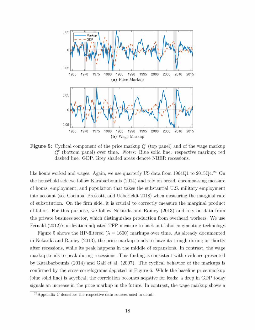
Figure 5: Cyclical component of the price markup ›p
t (top panel) and of the wage markup›
w
t(bottom panel) over time. Notes: Blue solid line: respective markup; red
dashed line: GDP. Grey shaded areas denote NBER recessions.
like hours worked and wages. Again, we use quarterly US data from 1964Q1 to 2015Q4.24 Onthe household side we follow Karabarbounis (2014) and rely on broad, encompassing measureof hours, employment, and population that takes the substantial U.S. military employmentinto account (see Cociuba, Prescott, and Ueberfeldt 2018) when measuring the marginal rateof substitution. On the firm side, it is crucial to correctly measure the marginal productof labor. For this purpose, we follow Nekarda and Ramey (2013) and rely on data fromthe private business sector, which distinguishes production from overhead workers. We useFernald (2012)’s utilization-adjusted TFP measure to back out labor-augmenting technology.
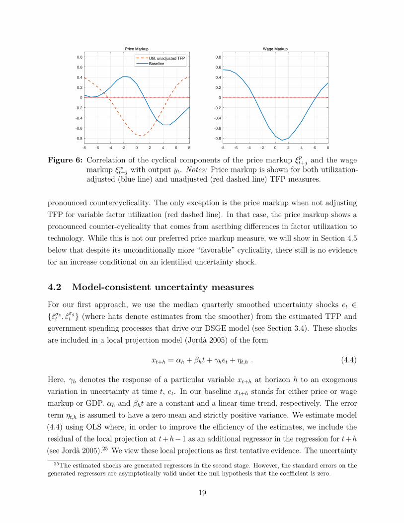
Figure 5 shows the HP-filtered (⁄ = 1600) markups over time. As already documentedin Nekarda and Ramey (2013), the price markup tends to have its trough during or shortlyafter recessions, while its peak happens in the middle of expansions. In contrast, the wagemarkup tends to peak during recessions. This finding is consistent with evidence presentedby Karabarbounis (2014) and Galí et al. (2007). The cyclical behavior of the markups isconfirmed by the cross-correlograms depicted in Figure 6. While the baseline price markup(blue solid line) is acyclical, the correlation becomes negative for leads: a drop in GDP todaysignals an increase in the price markup in the future. In contrast, the wage markup shows a
24Appendix C describes the respective data sources used in detail.
18
-8 -6 -4 -2 0 2 4 6 8
-0.8
-0.6
-0.4
-0.2
0
0.2
0.4
0.6
0.8
Price Markup
Util. unadjusted TFP
Baseline
-8 -6 -4 -2 0 2 4 6 8
-0.8
-0.6
-0.4
-0.2
0
0.2
0.4
0.6
0.8
Wage Markup
Figure 6: Correlation of the cyclical components of the price markup ›p
t+jand the wage
markup ›w
t+jwith output yt. Notes: Price markup is shown for both utilization-
adjusted (blue line) and unadjusted (red dashed line) TFP measures.
pronounced countercyclicality. The only exception is the price markup when not adjustingTFP for variable factor utilization (red dashed line). In that case, the price markup shows apronounced counter-cyclicality that comes from ascribing di�erences in factor utilization totechnology. While this is not our preferred price markup measure, we will show in Section 4.5below that despite its unconditionally more “favorable” cyclicality, there still is no evidencefor an increase conditional on an identified uncertainty shock.
4.2 Model-consistent uncertainty measures
For our first approach, we use the median quarterly smoothed uncertainty shocks et œ{Á
‡zt , Á
‡gt } (where hats denote estimates from the smoother) from the estimated TFP and
government spending processes that drive our DSGE model (see Section 3.4). These shocksare included in a local projection model (Jordà 2005) of the form
xt+h = –h + —ht + “het + ÷t,h . (4.4)
Here, “h denotes the response of a particular variable xt+h at horizon h to an exogenousvariation in uncertainty at time t, et. In our baseline xt+h stands for either price or wagemarkup or GDP. –h and —ht are a constant and a linear time trend, respectively. The errorterm ÷t,h is assumed to have a zero mean and strictly positive variance. We estimate model(4.4) using OLS where, in order to improve the e�ciency of the estimates, we include theresidual of the local projection at t+h≠1 as an additional regressor in the regression for t+h
(see Jordà 2005).25 We view these local projections as first tentative evidence. The uncertainty25The estimated shocks are generated regressors in the second stage. However, the standard errors on the
generated regressors are asymptotically valid under the null hypothesis that the coe�cient is zero.
19

Price Markup
0 2 4 6 8 10 12
quarters
-3
-2
-1
0
1
perc
ent
Wage Markup
0 2 4 6 8 10 12
quarters
-2
-1
0
1
2
perc
ent
GDP
0 2 4 6 8 10 12
quarters
-1.5
-1
-0.5
0
0.5
1
perc
ent
(a) Technology uncertainty.
Price Markup
0 2 4 6 8 10 12
quarters
-2
-1
0
1
perc
ent
Wage Markup
0 2 4 6 8 10 12
quarters
-1
0
1
2
3perc
ent
GDP
0 2 4 6 8 10 12
quarters
-1.5
-1
-0.5
0
0.5
perc
ent
(b) Government spending uncertainty.
Figure 7: Local projection responses to model-consistent two-standard deviation uncertaintyshocks. Notes: Shaded areas denote 90% confidence intervals based on Newey-West standard errors.
shocks are derived under the assumption that all heteroskedasticity in the residuals is theresult of exogenous uncertainty shocks. Insofar as there is endogenous uncertainty in theseobjects (see e.g. Caldara, Fuentes-Albero, Gilchrist, and Zakrajöek 2016; Plante, Richter,and Throckmorton 2018), we would be mis-measuring the shocks. We will turn to moresophisticated identification schemes below.
Figure 7 presents the IRFs to our model-consistent uncertainty shocks. As expected,an increase in technological uncertainty is associated with a drop in GDP. However, theconditional markup response in the data partially di�ers from the one predicted by themodel.26 On impact, the price markup falls. In contrast, the DSGE model implies that theprice markup quickly peaks and then declines back to its stochastic steady state as the e�ectof price stickiness subsides over time. The movement of the wage markup squares better withthe model: it increases after an uncertainty shock and then slowly declines back to steadystate. The evidence after a government spending uncertainty shock is not as conclusive, butalso does not lend strong support to the model mechanism.
26This conditional markup response is consistent with the conditional comovement Nekarda and Ramey(2013) found after other types of shocks, which also contradicted the sticky price model.
20

4.3 Two-step approach using broad macro uncertainty measure
The first set of impulse responses from the model-consistent uncertainty measures tentativelysuggests that the conditional behavior of the price markup is not consistent with the modelprediction. However, the bands were relatively wide. This is not entirely surprising as TFPmeasures are notoriously noisy and government spending shocks are hard to identify. Thus,we would like to rely on an uncertainty proxy that is still closely linked to the model conceptof uncertainty, but at the same time has a better signal-to-noise ratio. A measure satisfyingthis criterion has recently been proposed by Jurado et al. (2015, JLN henceforth). Theirmeasure is closely linked to the concept of forecast error uncertainty employed in businesscycle models, but relies on a broad information set to extract the signal.27 We think thatthis is currently the broadest and at the same time cleanest uncertainty measure available.28
We are ultimately interested in the dynamic response of markups to innovations, or“shocks”, to uncertainty. Given that the JLN uncertainty measure is available at monthlyfrequency while we only have quarterly markup data, we will employ a two-step procedurefollowing Kilian (2009) and Born, Breuer, and Elstner (2018). In the first step, to identifystructural uncertainty shocks, we follow Bloom (2009) and Jurado et al. (2015) and employa Cholesky-ordering within a monthly VAR framework. The structural shocks are thenaggregated to quarterly frequency by averaging the monthly shocks and, in the second step,fed into a local projection as in (4.4).29 We pursue this approach, because the monthly timehorizon of the VAR makes the recursive timing assumption underlying the identificationscheme more plausible than in a quarterly VAR.
Our sample ranges from 1964M1 to 2015M12. The variable vector Xt in our VAR contains1) real industrial production, 2) total non-farm employment, 3) real personal consumptionexpenditures, 4) the personal consumption expenditure deflator, 5) real new orders, 6) themanufacturing real wage, 7) hours worked in manufacturing, 8) the Wu and Xia (2016)shadow federal funds rate,30 9) the S&P 500 Index, 10) M2 money growth, and 11) the 1-step
27JLN stress that in order to measure uncertainty, it is important to purge the predictable component ofvolatility. They estimate a factor-based forecasting model on 279 monthly economic and financial time series.Given their estimated factors, they then compute forecast errors for 132 of these variables and subsequentlyuse the forecast errors to construct an uncertainty time series for each variable based on the assumption thatthese follow a stochastic volatility process. Their macroeconomic uncertainty measure is the common factorof the uncertainty connected to the individual variables. We use their one-period ahead forecast measure (i.e.h = 1, not to be confused with the forecast horizon in the local projection).
28Measures like the economic policy uncertainty index by Baker et al. (2016) have a very narrow focus, whilefinancial market-based measures like the VIX or realized (return) volatility are likely to be contaminated bychanges in risk aversion and financial market conditions (see e.g. Bekaert, Hoerova, and Duca 2013; Caldaraet al. 2016). We will employ these alternative measures in the robustness section.
29Using the average follows Kilian (2009). Readers worried about time aggregation are referred to themixed-frequency VAR below.
30We use this measure to alleviate concerns about the e�ective zero lower bound introducing a nonlinearity
21

Price Markup
0 2 4 6 8 10 12
quarters
-1
-0.5
0
0.5
1
pe
rce
nt
Wage Markup
0 2 4 6 8 10 12
quarters
0
1
2
3
pe
rce
nt
GDP
0 2 4 6 8 10 12
quarters
-1.5
-1
-0.5
0
0.5
pe
rce
nt
Figure 8: Local projection responses to a JLN-based two-standard deviation uncertaintyshock in the two-step model. Notes: Shaded areas denote 90% confidence intervalsbased on Newey-West standard errors.
ahead JLN uncertainty proxy.31 Formally, we estimate the following VAR using OLS
Xt = µ + –t + A(L)Xt≠1 + ‹t , (4.5)
where and µ and –t are a constant and time trend, respectively, A(L) is a lag polynomialof degree p=6, and ‹t
iid≥ (0, �). In terms of identification, we assume a lower-triangularmatrix B, which maps reduced-form innovations ‹t into structural shocks Át = B‹t. Theemployed ordering follows JLN and relies on economic aggregates not reacting within themonth to an increase in macroeconomic uncertainty, while uncertainty itself may react toother shocks. In Section 4.5 we confirm that our results are robust to ordering uncertaintybefore macroeconomic aggregates.
After averaging the monthly shocks and feeding them into the local projection model,the resulting IRFs are plotted in Figure 8. They corroborate our previous finding. After anuncertainty shock, the wage markup increases significantly, consistent with a precautionarywage setting motive as in the model. The same does not apply to the price markup, whichtends to decline.
4.4 Mixed-frequency VAR
The two-step approach comes at the disadvantage of not making full use of (relatively)high-frequency information. As mentioned before, the constructed markups are only availableat quarterly frequency. To use all available monthly information on the other variables, weassume that we cannot observe the monthly realizations of the markup measure and treatthese data as missing values. Following the Bayesian VAR framework outlined in Eraker
the VAR is not being able to capture. Using the e�ective federal funds rate instead yields very similar results.31See Appendix D.2 for a detailed description of the macro dataset and the transformations used for the
respective variables.
22

Macro uncertainty
0 10 20 30
0
0.02
0.04
un
itsReal industrial production
0 10 20 30
-2
-1.5
-1
-0.5
0
pe
rce
nt
Real wage
0 10 20 30-0.2
0
0.2
0.4
pe
rce
nt
Price markup
0 10 20 30
months
-0.6
-0.4
-0.2
0
0.2
0.4
pe
rce
nt
Wage Markup
0 10 20 30
months
0
0.5
1
1.5
2
pe
rce
nt
Total Markup
0 10 20 30
months
0
0.5
1
1.5
2
pe
rce
nt
Figure 9: IRFs to JLN-based two-standard deviation uncertainty shock in the mixed-frequency VAR. Notes: Bands are pointwise 90% HPDIs. The respective markupsare rotated into the VAR as the 12th variable. The macroeconomic uncertaintyindex is measured in arbitrary units and has a mean of 0.65. The first row andthe price markup response are from a VAR including the price markup. Theresponses of wage and total markup are from separate VARs (see text).
et al. (2015), we can then employ a Gibbs sampler to deal with these missing observations bysampling the missing data from their conditional distribution.
Our sample again ranges from 1964M1 to 2015M12, on which we estimate the 11-variableVAR in equation (4.5) with p = 6, but where we add our quarterly markup measures as anadditional twelfth variable observed every third month. Consistent with the model, we orderthe markups after the respective uncertainty measure so that markups can react on impact.We use a shrinking prior of the Independent Normal-Wishart type, where the mean andprecision are derived from a Minnesota-type prior.32 We use 90% highest posterior densityintervals (HPDIs) based on 1000 random posterior draws after burn-in.
We estimate three separate mixed-frequency VARs, one including the price markup, oneincluding the wage markup, and one including the total markup or “labor wedge”, i.e. thesum of the price and wage markup. Figure 9 presents the key impulse responses following atwo-standard deviation shock to macroeconomic uncertainty based on the three models.33 Aswith the model-consistent measure and the two-step approach, wage markups increase after
32See Appendix D.1 for details.33Appendix D.2 includes a full set of impulse responses of all three VARs.
23

an uncertainty shock but price markups fall.The bottom right panel of Figure 9 displays the total markup or “labor wedge”, i.e. the
sum of the price and wage markup. During the first few months, it is dominated by theprice markup response and slightly falls, before it becomes dominated by the wage markupand increases subsequently. As the figure shows, after an uncertainty shock the real wageincreases. This response, together with a fall in hours worked shown in the appendix, isperfectly consistent with a situation where the wage markup increases while the price markupstays flat (see the stylized labor market diagram in Figure 2).34 While the model does notpredict the same hump-shaped movement, it predicts the same countercyclical movement ofthe wage markup. At least in that regard, the data is consistent with the markup channelin NK models and the role of uncertainty shocks more generally. Empirically, most of themovement in the labor wedge seems to come from this margin. However, from the vantagepoint of the basic NK model with only sticky prices, the price markup response presents achallenge.
We also compute the posterior unconditional forecast error variance share explainedby the identified uncertainty shock. Uncertainty shocks account for about 13% of outputfluctuations, 15% of the wage markup, but only 8% of the price markup. Taken together,uncertainty shocks account for 11% of total labor wedge fluctuations (see Table D.5 in theappendix).
4.5 VAR-based robustness checks
While our results are robust across di�erent time-series approaches, one might wonder whetherthey depend on the ordering of variables in the VAR, the assumptions made to constructmarkups, or the chosen uncertainty proxy. We will address these concerns in the following.
Bloom (2009) VAR
Bloom (2009) considers a di�erent, 8-variable VAR where uncertainty is ordered second andmeasured by stock market volatility via the VIX. The reasoning behind this ordering is thatuncertainty shocks instantaneously influence stock market volatility and other prices andquantities, but that first moment shocks to stock-market levels are already controlled forwhen investigating the response to uncertainty shocks. In a first step, we check whether usingthe VIX instead of the JLN measure makes a di�erence in our VAR 11+1. The blue solidlines in Figure 10 confirm that the results are robust to this change.
34The model with only rigid wages also delivers an increase in the real wage and a drop in hours worked.
24

VIX
0 10 20 30
months
0
5
10
Ann. p.p
.
VAR 11
VAR 8
Price markup
0 10 20 30
months
-0.4
-0.2
0
0.2
0.4
perc
ent
Real industrial prod.
0 10 20 30
months
-1
-0.5
0
0.5
1
perc
ent
(a) Price Markup
VIX
0 10 20 30
months
0
5
10
Ann. p.p
.
VAR 11
VAR 8
Wage markup
0 10 20 30
months
-0.5
0
0.5
1
perc
ent
Real industrial prod.
0 10 20 30
months
-1
-0.5
0
0.5
1
perc
ent
(b) Wage Markup
Figure 10: IRFs to two-standard deviation uncertainty shocks measured via the VIX. Notes:Blue solid line: mixed-frequency 11+1-VAR with VIX ordered second-to-last;red dashed line: 8+1-Bloom (2009)-VAR with VIX ordered second (see text fordetails). Bands are pointwise 90% HPDIs computed for the 11+1-VAR.
Next, we investigate the original Bloom 8-variable VAR with uncertainty, measured bythe VIX, ordered second. We add our markup measure as the ninth variable.35 Results fromthe mixed-frequency estimation are included as red dashed lines in Figure 10. They are verysimilar to the baseline results, indicating that the ordering of the uncertainty measure is notcrucial for our results.36
Alternative markup measurements
In our baseline price markup measure, we employ the utilization-adjusted TFP measure ofFernald (2012), which results in an acyclical price markup. As a robustness check, we alsouse Fernald’s utilization-unadjusted TFP measure. This results in a strongly countercyclicalprice markup (see the red dashed line in the left panel of Figure 6), which, as Nekarda andRamey (2013) note, is very similar to the countercyclical markup measure constructed in Galíet al. (2007). Estimating our mixed-frequency VAR including this alternative price markupmeasure yields the IRFs reported in the upper left panel of Figure 11. The drop in the price
35See Appendix D.3 for a detailed variable listing and Figure D.10 for a full set of IRFs.36Figure D.11 shows that the IRFs when using the JLN-measure ordered second in the VAR are also similar.
Appendix D.4 provides the IRFs for various other measures of uncertainty.
25

Unadj. TFP-based
0 5 10 15 20 25 30 35
months
-0.4
-0.2
0
0.2
0.4
0.6p
erc
en
tNon-Financial, Tot. Comp.
0 5 10 15 20 25 30 35
months
-0.5
0
0.5
pe
rce
nt
Inv. Labor Share, Priv. Bus.
0 5 10 15 20 25 30 35
months
-0.5
0
0.5
pe
rce
nt
Prod. workers, Priv. Bus.
0 5 10 15 20 25 30 35
months
-0.4
-0.2
0
0.2
pe
rce
nt
Figure 11: Alternative price markup-IRFs to JLN-based two-standard deviation uncertaintyshocks in the mixed-frequency 11+1-VAR. Notes: See text for description ofmeasures. Bands are pointwise 90% HPDIs.
markup is less pronounced than in the baseline, but there is still no robust evidence for anincrease.
With respect to the price markup, one might also worry that the correction for overheadlabor, fixed costs, and a CES production function might be overdoing things. Figure 11therefore also reports the responses of three “conventional” markup measures based on asetup with no fixed costs and a Cobb-Douglas production function. In this case, the aggregateprice markup corresponds to the inverse labor share. The upper right panel of Figure 11displays the response of the price markup for the labor share based on total compensation inthe non-financial business sector (available from the NIPA tables). The lower left panel usesthe labor share of production and supervisory workers in the private business sector, whilethe lower right panel is based on production workers only in the private business sector, i.e.excludes overhead workers (both available from the BLS). In all three cases, the price markupsignificantly drops after an uncertainty shock. The first two measures, which are based on allworkers, tend to recover somewhat more quickly than the third measure, which accounts forthe presence of overhead labor as in the baseline. But even for the first two measures, we donot find a significant increase of the price markup within the first three years.
We also check whether our choice of the elasticity of substitution (EOS) between capitaland labor influences the dynamic response of the price markup. Unfortunately, the EOS
26

0 5 10 15 20 25 30 35
months
-0.5
0
0.5
1
1.5
2
2.5
3
pe
rce
nt
Wage Markup
Iso
GHH
CD habits
Iso Habits
Iso high RA
Iso low Frisch
SW (2007)
0 5 10 15 20 25 30 35
months
-0.4
-0.3
-0.2
-0.1
0
0.1
0.2
pe
rce
nt
Price Markup
0.5 (Base)
0.75
1
1.25
1.5
Figure 12: IRFs to JLN-based two-standard deviation uncertainty shocks in the mixed-frequency 11+1-VAR using a variety of measured markups. Notes: Left panel:price markups for range of EOS between capital and labor; right panel: wagemarkup for di�erent preference specifications (see text for details).
is di�cult to measure in the data and estimates range from 0.5 - 0.7 (e.g., Chirinko 2008;Oberfield and Raval 2019) to 1.25 and higher (e.g., Karabarbounis and Neiman 2014). Wetherefore compute price markups for parameterizations of the EOS ranging from 0.5 to 1.5and report the resulting IRFs to a two-standard-deviation uncertainty shock in the left panelof Figure 12. While larger values of the EOS correlate with smaller drops in the price markup,the general pattern of a fall in the price markup following an uncertainty shock stands.
We also check the robustness of the wage markup response with respect to the preferencespecification used (right panel of Figure 12). It first varies the functional form, keeping theFrisch elasticity at its baseline value of 1. The blue solid line shows separable isoelasticpreferences of the type U = log Ct ≠ ÂN
1+1/÷
t , while the red dashed line displays Greenwood,Hercowitz, and Hu�man (1988, GHH) preferences of the form U = log
1Ct ≠ ÂN
1+1/÷
t
2.37
Isoelastic preferences result in a wage markup that is more volatile over the business cycle (seealso Karabarbounis 2014), but that is otherwise similar to the baseline. The wage markupresponse with GHH preferences is also very similar to the baseline. The yellow dotted andthe violet dashed dotted lines display the Cobb-Douglas and the isoelastic preferences withexternal habits of 0.7, a common value in the literature. Habits cause a quicker and morepersistent increase in the wage markup. The next two lines display the e�ect of parametervariations for the case of isoelastic preferences. The green solid line uses a higher risk aversionparameter of ‡ = 2.5, while the cyan dashed line lowers the Frisch elasticity to 0.5. Inboth cases, the response of the wage markup almost doubles, but is qualitatively still thesame. Finally, the burgundy dotted line combines a higher risk aversion of 1.4, a lower Frisch
37The labor disutility parameter  only a�ects the constant in our markup measure and therefore can beset to 1 without loss of generality.
27

Table 3: Short-run response of BKM annual price markup to aggregate macroeconomicuncertainty shock
(1) (2) (3) (4) (5) (6) (7)h=0 0.340 0.198 0.288 0.490 -0.003 -0.241 -0.145
(0.482) (0.672) (0.393) (0.017) (0.314) (0.575) (0.310)h=1 1.616 1.787 1.561 0.377 1.081 1.220 0.818
(0.561) (0.737) (1.015) (1.889) (0.651) (0.675) (1.394)Hours All workers SE SE SE SE SE SEMPN Agg. Agg. SE SE Uninc SE SECons. PCE PCE PCE +CE Adj. PCE PCE PCE
Weight. Equal SE in CPS SE in CPS SE in CPS SE in CPS All in CPS Emp.Notes: Responses are in percent. Regressions based on years 1987-1993 and 1996-2012. Newey-West standarderrors are in parentheses. Hours are weekly. MPN refers to how the marginal product is measured: “Agg.”denotes the NIPA labor productivity measure, “SE” denotes self-employed income per hour, “Uninc” denotesunincorporated self-employed income per hour. “Cons.” denotes the respective consumption measure. PCE:NIPA aggregate real expenditures on nondurables and services. CE adjustment incorporates consumptionfor the self-employed versus all persons from the Consumer Expenditure Surveys. Weighting schemes: “SEin CPS’ weights all self-employed in the CPS equal, “All in CPS’ weights self-employed to achieve mirrorindustry structure of all workers in the CPS, and “Emp.” reweights with the share of self-employed withemployees (see BKM for details).
elasticity of 0.5, and external habits of 0.71 as estimated for the US in Smets and Wouters(2007). The response of the wage markup in this case combines the quick and drawn outincrease of the external habit case with the higher peak response of the high risk aversion/lowFrisch elasticity cases.
4.6 Price markup based on self-employed and new jobs formed
The previous analyses have relied on a measure of average hourly earnings, which would bethe appropriate measure of firms’ marginal cost of labor if transactions took place in perfectlycompetitive spot markets. But due to implicit long-term contracts between firms and workersthis measure of earnings may not play an allocative role. For this reason, Bils et al. (2018,BKM) have recently investigated the labor wedge of self-employed people along the intensivemargin. Arguably, no wage rigidities and labor market distortions a�ect their decision tosupply labor to their own business. In this case the wage markup is zero and the labor wedgecoincides with the price markup. The share of self-employed in nonagricultural industries isroughly 10%. The BKM data is based on the Annual Social and Economic Supplements tothe CPS from 1987 to 2012 with a gap in 1994 and 1995 due to a CPS sample redesign. Thewedge construction assumes separable isoelastic preferences with a Frisch elasticity of unityand an intertemporal elasticity of substitution of 0.5.
In Table 3, we investigate the e�ect of uncertainty shocks on the BKM annual intensive
28

margin labor wedges during the first two years after the shock. The aggregate uncertaintyshock is constructed as the annual average of the monthly uncertainty shocks estimated usingthe VAR (4.5). The first column displays the results based on hours, labor productivity, andconsumption of all workers, not just the self-employed.38 The response therefore needs tobe interpreted as the total markup. Consistent with our previous findings based mostly onquarterly NIPA data, it shows a delayed increase. The next columns subsequently replace theaggregate components of the wedge computation by measures specific to the self-employed.Most importantly, starting with the second column the total hours measure is replaced bythe one for the self-employed. The resulting wedge can therefore be interpreted as the pricemarkup. As the second column shows, we find a significant increase of the price markup afterone year, consistent with the markup channel. The third column then replaces the aggregatelabor productivity measure by one for the self-employed, that is business income divided byhours. This change causes the price markup increase to become insignificant. The reason maybe that, as argued in BKM, this measure tends to understate the cyclicality of the labor wedge.The fourth column adjusts the previously used aggregate consumption measure by a measureof consumption for the self-employed derived from the CPS. Self-employed consumption ismore cyclical, which causes the estimated price markup to increase significantly on impact, butrevert more quickly. The fifth column again uses aggregate consumption, but considers onlynon-incorporated businesses to avoid issues with reporting of business income as corporateprofits. We find a marginally significant increase in the price markup after one year. Finally,columns (6) and (7) use a di�erent weighting scheme. Column (6) reweights observations byindustry in order to achieve a weighting of self-employed by industry that mirrors the one ofall employees.39 This assures a similar aggregate cyclical exposure of the self-employed wedgemeasure as for the whole worker population. This reweighting hardly makes a di�erence. Westill only find a marginally significant increase in the wedge after one year. Finally, column(7) reweights observations by the share of self-employed with employees. The goal is to giveless weight to self-employed people that might just contract with one employer and are thusquasi-employees with all associated rigidities. In this case, the price markup increase afterone year becomes insignificant.
Summarizing, estimating the response of the price markup based on an annual dataset ofself-employed persons yields some tentative evidence for the presence of the markup channel.One year after the shock, the point estimate is consistently positive. However, the significanceof this increase in the price markup depends on the exact specification used.
38For details on the construction of the respective wedges, we refer the reader to BKM.39For example, if self-employment is twice as likely in construction than overall, self-employed in construction
only receive a weight of one half.
29

Finally, we turn to the extensive labor margin. Most representative agent models investi-gating the e�ect of uncertainty shocks only feature an intensive margin of labor adjustmentand rely on a measure of average hourly earnings to represent the opportunity cost of firms(e.g. the estimations in Born and Pfeifer 2014a; Fernández-Villaverde et al. 2015). In theory,if this wage measure were allocative, e.g. if all workers were hired in spot markets, markupsbased on it should return the same result as any other margin of adjustment available to thefirm. However, there are well-documented reasons like implicit long-term contract concernsthat may prevent wages of existing jobs from adjusting in a frictionless way (see e.g. Basuand House 2016). We investigate whether our findings change if we consider the extensivemargin adjustment and analyze a firm’s decisions when forming new jobs.
For this purpose, we rely on two quarterly extensive margin price markups constructedin BKM for the period from 1987 to 2012.40 Instead of relying on average hourly earningsof all workers, the two measures follow Kudlyak (2014) and employ the wage of new hiresand the user cost of labor, respectively.41 Both cost measures are arguably more relevant forthe firm’s hiring decisions than average wages. BKM obtain these two measures based ontheir respective semi-elasticities and the one of average hourly earnings with respect to theunemployment rate. While average wages fall by 1.5% for each percentage point increase inunemployment, wages of newly hired workers fall by 3% and the user cost by 4.5%. Thisinformation allows constructing the wage of new hires and the user cost of labor by adjustingaverage hourly earnings for the respective di�erent comovement with respect to the observedunemployment series.
The impulse responses of the two extensive margin price markups are shown in Figure 13.The left panel shows the response of the price markup when using the wage of new hires asthe relevant firm cost measure. After an initial, insignificant drop, the price markup increasessignificantly after about one year. The right panel displays the price markup based on theuser cost of labor. It also increases in a hump-shaped manner, but already becomes significantafter about 6 months and exhibits a larger peak. Thus, these tentative measures of extensivemargin price markups provide the strongest evidence yet for the presence of a markup channel.The results suggest that recent modeling e�orts combining search-and-matching modelswith uncertainty shocks (Leduc and Liu 2016; den Haan et al. 2020) may be a particularlypromising avenue for obtaining data-consistent model responses to uncertainty shocks.
40We verified that our baseline intensive margin results are unaltered if we restrict our analysis to thisshorter sample period. For details on the construction of extensive margin price markups, we refer interestedreaders to the original paper.
41Kudlyak (2014) defines the user cost as the expected di�erence between the present value of wages paidto a worker hired in period t and that hired in t + 1. If the labor market were a spot market, this di�erencewould simply be the wage.
30

Ext. Margin, New Hires
0 5 10 15 20 25 30 35
months
-0.5
0
0.5
1
1.5
2
pe
rce
nt
Ext. Margin, User Cost
0 5 10 15 20 25 30 35
months
-0.5
0
0.5
1
1.5
2
pe
rce
nt
Figure 13: IRFs to JLN-based two-standard deviation uncertainty shocks in the mixed-frequency 11+1-VAR using the BKM extensive margin price markups basedon the wage of new hires (left panel) and the user cost of labor (right panel).Sample range: 1987M1:2012M12.
However, these findings come with two important caveats. First, while BKM were onlyinterested in the unconditional cyclicality of price markups, their mechanical unemployment-based adjustment of average hourly earnings is problematic in our context of a conditionalanalysis. It carries the risk of introducing a spurious e�ect of uncertainty shocks. Empiri-cally, uncertainty shocks tend to exhibit a significant e�ect on unemployment, which – byconstruction – will a�ect the measurement of new hire wages and the user cost of labor. Forthis reason, we consider the evidence presented above to be tentative and pointing towardsthe need for further investigation.
Second, and perhaps even more importantly, it needs to be pointed out that – in contrastto the other markup measures considered in the present paper – constructing price markupsin a search-and-matching framework requires dynamic equilibrium conditions. Therefore,results will strongly depend on the model assumptions and the employed empirical models toinfer expectations about future variables from the data. We leave an investigation of theseissues for future research.
5 Industry-level evidenceIn the previous section, we have documented that there is only mixed empirical evidencefor price markup increases after uncertainty shocks at the aggregate level. In this sectionwe dig deeper, turning to disaggregated industry-level evidence to investigate whether themodel-predicted price markup response may simply be hidden by i) heterogeneity in pricestickiness at the industry level or ii) measuring price markups along the labor margin insteadof the potentially more flexible intermediate input margin. The results in this section need
31

to be interpreted with caution. First, the markup channel provides clear-cut predictionsfor aggregate markups based on aggregate equilibrium conditions (what BKM have calledthe representative-agent labor wedge). Strictly speaking it is silent on what happens at amore disaggregated level. Aggregation from the average markup of firms or industries to themarkup of the average firm is not trivial (see e.g. De Loecker et al. 2020). However, we expectthis issue to be less problematic if aggregation is at the industry rather than the firm level.42
Second, input-output-relationships between sectors can lead to non-trivial interactions withnominal rigidities (see e.g. Pasten, Schoenle, and Weber 2018). We abstract from this issueas it is beyond the scope of the present paper, but think it deserves more future attention.Despite these limitations, we still consider the industry-level analysis to be an additionaluseful piece of evidence.
5.1 Constructing industry-specific markups
Based on the NBER CES Manufacturing Industry Database (Becker, Gray, and Marvakov2016; Bartelsman and Gray 1996) we construct price markups and output measures at thefour digit SIC-industry level (see Appendix C.5 for details). As we have argued before, arobust result of representative agent models with convex adjustment costs is that negativeoutput e�ects of uncertainty are directly related to nominal stickiness. As a first pass atthe data, we therefore estimate the contemporaneous response of real output for each SIC4industry and plot it against average price durations for these industries. To compute thisresponse, for each industry we regress the log of real output yt on the aggregate uncertaintyshock, a constant, and a linear time trend:
log(yt) = –0 + –1t + –2et + Át . (5.1)
Again, the aggregate uncertainty shock et is the annual average of the monthly uncertaintyshocks estimated using the VAR (4.5). Implied average price durations are computed for SIC4industries based on the estimated New Keynesian Phillips Curves in Petrella and Santoro(2012).43 Figure 14 plots the resulting estimates –2 against average price durations. Theredoes not seem to be a linear relationship between price stickiness and the output e�ects ofuncertainty shocks. The regression line is flat and the slope coe�cient is insignificant at the5% level.
42The di�erent level of aggregation is also the reason why BKM’s industry-level analysis does not reveal atrend in the average markup, while De Loecker et al. (2020)’s firm-level analysis does.
43For that purpose, we translate their estimated slope of the New Keynesian Phillips Curve into a Calvoprice duration parameter, using — = 0.99.
32

0 2 4 6 8 10
Price duration (years)
-0.04
-0.02
0
0.02
0.04
0.06
Conte
mpora
neous
unce
rtain
ty e
ffect
on o
utp
ut
y=0.001-0.000x
Figure 14: Implied average price duration at the SIC4 industry-level vs. output e�ects ofaggregate uncertainty shock. Notes: Implied average price durations are basedon Petrella and Santoro (2012); output e�ect estimates based on regression (5.1)using mean annual JLN shocks from VAR-11.
5.2 Regression evidence
As price stickiness per se does not seem seem to be related to the output e�ects of uncertainty,we now investigate the markup channel itself. Specifically, we run a panel version of the localprojection (4.4)
xi,t+h = –i,h + —i,ht + “het + ÷i,t+h . (5.2)
Again, “h denotes the response of a particular variable xt+h at horizon h to an exogenousvariation in uncertainty at time t, et, where xt+h is either the industry-specific price markupor industry-specific real output. –i,h and —i,ht are industry-specific constant and time trend,respectively. Given the short annual panel, we restrict ourself to h = 0 and h = 1. Theresults of the pooled OLS regression are shown in Table 4. Standard errors are robust toserial and cross-sectional correlation based on the approach by Driscoll and Kraay (1998).Qualitatively, the results look quite similar to the aggregate evidence. Industry-level output(first column) declines after a one-standard deviation uncertainty shock. While the pricemarkup based on a CES production function and production-worker compensation shows aninitial, marginally significant increase (which disappears after year), markups constructedusing all workers (column [2]) and a Cobb-Douglas production function (column [3]) fall(insignificantly) on impact.
In a final robustness check, we use price markups constructed by BKM based on the shareof intermediate inputs. Arguably, the markup measured along the intermediate inputs margin
33

Table 4: Short-run response of industry-level price markup to aggregate macroeconomicuncertainty shock
Output Markup[1] [2] [3] [4]
h=0 ≠1.45 1.61 ≠0.10 ≠0.45 ≠0.44(1.73) (0.94) (0.36) (0.41) (0.37)
h=1 ≠3.13 0.66 ≠0.31 ≠0.24 0.78(1.20) (0.68) (0.24) (0.20) (0.67)
Sectors 459 451 458 458 60Observations 21463 21197 21416 21416 1500
Notes: Responses, based on local projection (5.2), are in percent. Markup [1]: based on CES productionfunction and production-worker compensation; markup [2]: based on CES production function and all-workercompensation; markup [3]: based on Cobb-Douglas production function and production-worker compensation;markup [4]: markup based on BKM intermediates share. Driscoll-Kray standard errors in parentheses.
is less a�ected by the type of implicit contracting that may make wages not allocative.44
These markups, based on the KLEMS database, are available for 60 sectors, 42 of thoseoutside of manufacturing, on an annual basis from 1987 to 2012. The results are shown inthe last column of Table 4 and corroborate our earlier findings of no consistent evidence for aprice markup increase after uncertainty shocks.
6 ConclusionThe question of the markup channel as an empirically plausible transmission mechanismof uncertainty shocks into the macroeconomy is highly relevant for the policy debate giventhat the supposedly negative influence of policy uncertainty has become a recurring themein the political discourse. With much of the model-based evidence featuring this supposedtransmission mechanism, it is of paramount importance to subject it to a rigorous empiricalassessment.
We construct a DSGE model to measure markups and to generate theoretical markupresponses following uncertainty shocks. We then provide econometric evidence on the responseof markups to identified uncertainty shocks. The model-implied e�ects of uncertainty shocksare generally much smaller than their empirical counterparts. This is due to i) employinga micro-estimate-based, conservative model parameterization and ii) our estimated drivingprocesses not featuring large and persistent increases in uncertainty.
44Following the evidence in BKM that their measured markup does not contain a trend, we do not includea trend in the regression.
34

Contrary to the model’s prediction, price markups do not consistently increase afteridentified uncertainty shocks. The only tentative evidence for an increase in price markups wecan find is for price markups measured along the extensive margin. However, wage markupsincrease after uncertainty shocks, suggesting that sticky wages play a more important role inthe transmission of aggregate uncertainty shocks to economic variables than sticky prices.45
Of course it is important to understand why model-consistently measured price markupsdo not increase as predicted by the model. We can think of at least three potential reasons.First, the model assumes that any demand always has to be satisfied. In reality, firms mightavoid having to satisfy demand at disadvantageous prices by “being out of stock”. Thispotential violation of a crucial model assumption may be one reason why we find less evidenceof a precautionary pricing for firms. Second, instead of hiking their prices, firms may careabout protecting their customer base and invest into market shares.46 However, while theevidence in Gilchrist, Schoenle, Sim, and Zakrajöek (2017) is consistent with the relevanceof customer markets, it suggests that, together with empirically realistic financial frictions,customer markets actually strengthen the countercyclical model behavior of markups.
Finally, average wages may not be allocative. When we tentatively analyze price markupsmeasured along the extensive margin, we find that they increase. The intensive margin-onlylabor market structure in the spirit of Erceg et al. (2000) embedded in most medium-scaleNK models may therefore require to be augmented by an extensive margin. A crucial openquestion in that regard is how to resolve the fundamental indeterminacy of wages withinthe bargaining set. The exact type of wage setting mechanism employed is important forunderstanding the e�ects of uncertainty shocks (see den Haan et al. 2020) and the behaviorof model-consistent wage and price markups. A rigorous analysis of this nexus must be leftfor future research.
45See also Barattieri, Basu, and Gottschalk (2014) and Daly and Hobijn (2014) on the importance of stickywages.
46We thank an anonymous referee for suggesting this possibility.
35
ReferencesAdjemian, Stéphane et al. (2011). “Dynare: reference manual, version 4”. Dynare Working
Papers 1. CEPREMAP.Alessandri, Piergiorgio and Haroon Mumtaz (2019). “Financial regimes and uncertainty
shocks”. Journal of Monetary Economics 101, 31–46.Altig, David, Lawrence J. Christiano, Martin Eichenbaum, and Jesper Lindé (2011). “Firm-
specific capital, nominal rigidities and the business cycle”. Review of Economic Dynamics14 (2), 225–247.
Anderson, Eric, Sergio Rebelo, and Arlene Wong (2018). “Markups across space and time”.NBER Working Papers 24434.
Andreasen, Martin M., Jesús Fernández-Villaverde, and Juan F. Rubio-Ramírez (2018). “Thepruned state-space system for non-linear DSGE models: theory and empirical applications”.Review of Economic Studies 85 (1), 1–49.
Bachmann, Rüdiger and Christian Bayer (2013). “‘‘Wait-and-see” business cycles?” Journalof Monetary Economics 60 (6), 704–719.
Bachmann, Rüdiger, Ste�en Elstner, and Eric R. Sims (2013). “Uncertainty and economic ac-tivity: evidence from business survey data”. American Economic Journal: Macroeconomics5 (2), 217–249.
Baker, Scott R., Nicholas Bloom, and Steven J. Davis (2016). “Measuring economic policyuncertainty”. Quarterly Journal of Economics 131 (4), 1593–1636.
Balleer, Almut, Nikolay Hristov, and Dominik Menno (2017). “Financial constraints andnominal price rigidities”. CEPR Discussion Paper 11790.
Barattieri, Alessandro, Susanto Basu, and Peter Gottschalk (2014). “Some evidence on theimportance of sticky wages”. American Economic Journal: Macroeconomics 6 (1), 70–101.
Bartelsman, Eric J. and Wayne Gray (1996). “The NBER Manufacturing ProductivityDatabase”. NBER Technical Working Paper 205.
Ba�kaya, Yusuf Soner, Timur Hülagü, and Hande Kü�ük (2013). “Oil price uncertainty in asmall open economy”. IMF Economic Review 61 (1), 168–198.
Basu, Susanto and Brent Bundick (2017). “Uncertainty shocks in a model of e�ective demand”.Econometrica (85) (3), 937–958.
Basu, Susanto and Christopher L. House (2016). “Allocative and remitted wages: new factsand challenges for Keynesian models”. Ed. by John B. Taylor and Harald Uhlig. Vol. 2.Handbook of Macroeconomics. Elsevier. Chap. 16, 297–354.
36

Becker, Randy, Wayne Gray, and Jordan Marvakov (2016). “NBER-CES ManufacturingIndustry Database: technical notes”. Cambridge, MA, National Bureau of EconomicResearch. Cambridge, MA, National Bureau of Economic Research.
Bekaert, Geert, Marie Hoerova, and Marco Lo Duca (2013). “Risk, uncertainty and monetarypolicy”. Journal of Monetary Economics 60 (7), 771–788.
Berger, David, Ian Dew-Becker, and Stefano Giglio (2020). “Uncertainty shocks as second-moment news shocks”. Review of Economic Studies 87 (1), 40–76.
Bianchi, Francesco, Howard Kung, and Mikhail Tirskikh (2019). “The origins and e�ects ofmacroeconomic uncertainty”. CEPR Discussion Paper 13450.
Bils, Mark, Peter J. Klenow, and Benjamin A. Malin (2018). “Resurrecting the role of theproduct market wedge in recessions”. American Economic Review 108 (4-5), 1118–46.
Bloom, Nicholas (2009). “The impact of uncertainty shocks”. Econometrica 77 (3), 623–685.Born, Benjamin, Sebastian Breuer, and Ste�en Elstner (2018). “Uncertainty and the Great
Recession”. Oxford Bulletin of Economics and Statistics 80 (5), 951–971.Born, Benjamin and Johannes Pfeifer (2014a). “Policy risk and the business cycle”. Journal
of Monetary Economics 68, 68–85.(2014b). “Risk matters: the real e�ects of volatility shocks: Comment”. American
Economic Review 104 (12), 4231–4239.(2020). “The New Keynesian Wage Phillips Curve: Calvo vs. Rotemberg”. Macroeco-
nomic Dynamics 24 (5), 1017–1041.Caldara, Dario, Christina Fuentes-Albero, Simon Gilchrist, and Egon Zakrajöek (2016). “The
macroeconomic impact of financial and uncertainty shocks”. European Economic Review88, 185–207.
Carriero, Andrea, Haroon Mumtaz, Konstantinos Theodoridis, and Angeliki Theophilopoulou(2015). “The impact of uncertainty shocks under measurement error: a proxy SVARapproach”. Journal of Money, Credit and Banking 47 (6), 1223–1238.
Castelnuovo, Efrem (2019). “Domestic and global uncertainty: a survey and some new results”.CESifo Working Paper 7900.
Castelnuovo, Efrem and Giovanni Pellegrino (2018). “Uncertainty-dependent e�ects of mone-tary policy shocks: a New-Keynesian interpretation”. Journal of Economic Dynamics andControl 93, 277–296.
Cesa-Bianchi, Ambrogio and Emilio Fernandez-Corugedo (2018). “Uncertainty, financialfrictions, and nominal rigidities: a quantitative investigation”. Journal of Money, Creditand Banking 50 (4), 603–636.
Chari, V. V., Patrick J. Kehoe, and Ellen R. McGrattan (2007). “Business cycle accounting”.Econometrica 75 (3), 781–836.
37

Chirinko, Robert S. (2008). “‡: the long and short of it”. Journal of Macroeconomics 30 (2),671–686.
Chirinko, Robert S. and Debdulal Mallick (2017). “The substitution elasticity, factor shares,and the low-frequency panel model”. American Economic Journal: Macroeconomics 9 (4),225–53.
Christiano, Lawrence J., Martin Eichenbaum, and Charles L. Evans (2005). “Nominal rigiditiesand the dynamic e�ects of a shock to monetary policy”. Journal of Political Economy113 (1), 1–45.
Christiano, Lawrence J., Roberto Motto, and Massimo Rostagno (2014). “Risk shocks”.American Economic Review 104 (1), 37–65.
Chugh, Sanjay K. (2016). “Firm risk and leverage-based business cycles”. Review of EconomicDynamics 20, 111–131.
Cociuba, Simona E., Edward C. Prescott, and Alexander Ueberfeldt (2018). “US hours atwork”. Economics Letters 169, 87–90.
Cúrdia, Vasco, Andrea Ferrero, Ging Cee Ng, and Andrea Tambalotti (2015). “Has U.S.monetary policy tracked the e�cient interest rate?” Journal of Monetary Economics 70,72–83.
Daly, Mary C. and Bart Hobijn (2014). “Downward nominal wage rigidities bend the PhillipsCurve”. Journal of Money, Credit and Banking 46 (S2), 51–93.
De Loecker, Jan, Jan Eeckhout, and Gabriel Unger (2020). “The rise of market power andthe macroeconomic implications”. Quarterly Journal of Economics 135 (2), 561–644.
den Haan, Wouter, Lukas B. Freund, and Pontus Rendahl (2020). “Volatile hiring: uncertaintyin search and matching models”. CEPR Discussion Paper 14630.
Diercks, Anthony M., Alex Hsu, and Andrea Tamoni (2019). “When it rains it pours: cascadinguncertainty e�ects”. Mimeo.
Driscoll, John C. and Aart C. Kraay (1998). “Consistent covariance matrix estimation withspatially dependent panel data”. Review of Economics and Statistics 80 (4), 549–560.
Eraker, Bjørn, Ching Wai (Jeremy) Chiu, Andrew T. Foerster, Tae Bong Kim, and Hernán D.Seoane (2015). “Bayesian Mixed Frequency VARs”. Journal of Financial Econometrics13 (3), 698–721.
Erceg, Christopher J., Dale W. Henderson, and Andrew T. Levin (2000). “Optimal monetarypolicy with staggered wage and price contracts”. Journal of Monetary Economics 46 (2),281–313.
Fernald, John (2012). “A quarterly, utilization-adjusted series on total factor productivity”.Federal Reserve Bank of San Francisco Working Paper 2012-19.
38
Fernández-Villaverde, Jesús, Pablo A. Guerrón-Quintana, Keith Kuester, and Juan F. Rubio-Ramírez (2015). “Fiscal volatility shocks and economic activity”. American EconomicReview 105 (11), 3352–3384.
Galí, Jordi, Mark Gertler, and J. David López-Salido (2007). “Markups, gaps, and the welfarecosts of business fluctuations”. Review of Economics and Statistics 89 (1), 44–59.
Gilchrist, Simon, Raphael Schoenle, Jae Sim, and Egon Zakrajöek (2017). “Inflation dynamicsduring the financial crisis”. American Economic Review 107 (3), 785–823.
Greenwood, Jeremy, Zvi Hercowitz, and Gregory W. Hu�man (1988). “Investment, capacityutilization, and the real business cycle”. American Economic Review 78 (3), 402–17.
Hall, Robert E. (1997). “Macroeconomic fluctuations and the allocation of time”. Journal ofLabor Economics 15 (1), 223–250.
Jones, John Bailey (2002). “Has fiscal policy helped stabilize the postwar U.S. economy?”Journal of Monetary Economics 49 (4), 709–746.
Jordà, Òscar (2005). “Estimation and inference of impulse responses by local projections”.American Economic Review 95 (1), 161–182.
Jurado, Kyle, Sydney C. Ludvigson, and Serena Ng (2015). “Measuring uncertainty”. AmericanEconomic Review 105 (3), 1177–1216.
Karabarbounis, Loukas (2014). “The labor wedge: MRS vs. MPN”. Review of EconomicDynamics 17 (2), 206–223.
Karabarbounis, Loukas and Brent Neiman (2014). “The global decline of the labor share”.Quarterly Journal of Economics 129 (1), 61–103.
Kilian, Lutz (2009). “Not all oil price shocks are alike: disentangling demand and supplyshocks in the crude oil market”. American Economic Review 99 (3), 1053–69.
Kudlyak, Marianna (2014). “The cyclicality of the user cost of labor”. Journal of MonetaryEconomics 68, 53–67.
Kuester, Keith (2010). “Real price and wage rigidities with matching frictions”. Journal ofMonetary Economics 57 (4), 466–477.
Leduc, Sylvain and Zheng Liu (2016). “Uncertainty shocks are aggregate demand shocks”.Journal of Monetary Economics 82, 20–35.
Levitt, Steven D., John List, and Chad Syverson (2013). “Toward an understanding oflearning by doing: evidence from an automobile assembly plant”. Journal of PoliticalEconomy 121 (4), 643–681.
Mumtaz, Haroon and Francesco Zanetti (2013). “The impact of the volatility of monetarypolicy shocks”. Journal of Money, Credit and Banking 45 (4), 535–558.
Nakamura, Emi and Jón Steinsson (2008). “Five facts about prices: a reevaluation of menucost models”. Quarterly Journal of Economics 123 (4), 1415–1464.
39

Nakamura, Emi and Jón Steinsson (2013). “Price rigidity: microeconomic evidence andmacroeconomic implications”. Annual Review of Economics 5 (1), 133–163.
Nekarda, Christopher J. and Valerie A. Ramey (2013). “The cyclical behavior of the price-costmarkup”. NBER Working Papers 19099.
Oberfield, Ezra and Devesh Raval (2019). “Micro data and macro technology”. Mimeo.Princeton University.
Oh, Joonseok Jason (forthcoming). “The propagation of uncertainty shocks: Rotemberg vs.Calvo”. International Economic Review.
Pasten, Ernesto, Raphael S. Schoenle, and Michael Weber (2018). “Price rigidity and theorigins af aggregate fluctuations”. CESifo Working Paper 7190.
Petrella, Ivan and Emiliano Santoro (2012). “Inflation dynamics and real marginal costs:new evidence from U.S. manufacturing industries”. Journal of Economic Dynamics andControl 36 (5), 779–794.
Plante, Michael, Alexander W. Richter, and Nathaniel A. Throckmorton (2018). “The zerolower bound and endogenous uncertainty”. Economic Journal 128 (611), 1730–1757.
Richter, Alexander W. and Nathaniel A. Throckmorton (2016). “Is Rotemberg pricing justifiedby macro data?” Economics Letters 149, 44–48.
Rotemberg, Julio J. and Michael Woodford (1999). “The cyclical behavior of prices and costs”.Handbook of Macroeconomics. Ed. by John B. Taylor and Michael Woodford. Vol. 1B.North-Holland, 1051–1135.
Smets, Frank and Rafael Wouters (2007). “Shocks and frictions in US business cycles: aBayesian DSGE approach”. American Economic Review 97 (3), 586–606.
Wu, Jing Cynthia and Fan Dora Xia (2016). “Measuring the macroeconomic impact ofmonetary policy at the zero lower bound”. Journal of Money, Credit and Banking 48(2-3), 253–291.
40