uncertainty in global sourcing learning, sequential

CESifo and AUEB-LINER Conference on

The Role of Institutions and Policies in Firm Exporting Munich, 5–6 November 2020

Uncertainty in Global Sourcing

Learning, sequential offshoring, and selection

patterns Mario Larch and Leandro Navarro

Uncertainty in Global Sourcing∗

Learning, sequential offshoring, and selection patterns.

.- Preliminary draft -

Mario LarchUniversity of Bayreuth

Leandro NavarroJohannes Gutenberg University Mainz

October 28, 2020

Abstract

Institutions play an important role shaping the multinational firms’ sourcing decisions world-wide. We analyse firms’ sourcing decisions when they face uncertainty about institutional conditionsabroad. In a North-South model, we find that firms exploit informational externalities, which allowthem to better assess their offshoring potential by observing other firms’ behaviour. A sequential off-shoring equilibrium path drives the economy to the perfect information steady state, led by the mostproductive firms in the market. Finally, the extension to multiple countries shows multiple equilibriawith implications in terms of welfare and allocation of production across countries. The prior beliefsand the informational spillovers drive the sectoral specialisation of countries, and thence become asource of their comparative advantages. Using firm-level data from Colombia, we build a direct mea-sure for the informational spillovers, and test the main predictions of the model from two approaches.With a conditional probability model, we test for the determinants of the offshoring decisions andthe location choices, while by a survival analysis approach we test for the timing dimension of thosedecisions.

Keywords: Multinational firms, global sourcing, supply chain, institutions, uncertainty, information externalities,spillovers, learning, sequential offshoring, selection patterns, comparative advantages, multiple equilibria, sur-vival analysis.JEL: D81, D83, F10, F14, F23

1 Introduction

Intermediate inputs explain a substantial share of global trade, revealing a deep transformation of thestructure of international trade. The geographical vertical disintegration of the supply chains makes evi-dent that sourcing strategies have become global, arousing the interest of many scholars to understand thedeterminants of the offshoring activity, the sourcing strategies of multinational firms, and their role in theorganisation of international trade1. Recent literature has focused the attention on how institutions affectthe firms’ investment decisions, their organisational structures and technology choices (Helpman, 2006;Acemoglu et al., 2007; Antras and Helpman, 2008; Antras and Chor, 2013), as well as the institutionaldeterminants of countries’ comparative advantages (Costinot, 2009; Acemoglu et al., 2007; Nunn, 2007;Levchenko, 2007).∗Acknowledgements to be added.1Hummels et al. (2001); Helpman (2006); Antras and Helpman (2004, 2008); Grossman and Helpman (2005); Grossman

and Rossi-Hansberg (2008); Alfaro and Charlton (2009); Nunn and Trefler (2008, 2013); Antras and Yeaple (2014); Antras(2015); Ramondo et al. (2015); Antras et al. (2017)

1

However, while firms take usually their sourcing decisions under uncertainty, in particular aboutthe prevailing conditions (e.g. institutions) in foreign countries, most of these studies characterise thesedecisions under perfect information. A clear case of uncertainty arises when firms consider sourcing fromlocations where they have never been active before2. But it may also emerge with respect to locationswhere firms have had some experience in the past. For instance, after the implementation of an ambitiousinstitutional reform by a foreign government, firms may face doubts about the true scope of the reform,inducing uncertainty about the ex-post-reform prevailing institutional conditions.

The primary goal of this paper is to understand how the existence of prior uncertainty about theinstitutional fundamentals in foreign countries may affect the firms’ sourcing decisions, in particularoffshoring, and comprehend its implications in terms of the organisation of the firm and the supplychain, the sectoral specialisation of countries, and the respective welfare consequences.

The paper builds mainly from the literature on global sourcing with heterogeneous firms, in partic-ular the models developed by Antras and Helpman (2004, 2008), and complements the approaches ofGrossman and Helpman (2005) and Antras et al. (2017) where the focus is on the location dimensionof the offshoring decisions. The main departure from this literature consists in introducing institutionaluncertainty as an ambiguous knowledge about the per-period offshoring organisational fixed costs. Forsimplicity, in order to focus in the location dimension of the sourcing decisions, we consider the case ofcomplete contracts3.

Up to our knowledge, this is the first paper in the global sourcing literature to introduce uncertaintyin the form of a diffuse knowledge about conditions abroad, and to allow firms to learn about theiroffshoring potential by exploiting informational externalities obtained by observing the behaviour of theother firms.

There is a small but growing literature on uncertainty in global sourcing decisions, but the attentionhas centered on how the exposure to shocks affects firms’ choices (Carballo, 2016; Kohler et al., 2018)4.In those cases, the firms optimise their sourcing strategy with a perfect knowledge of the distributionsof shocks, i.e. the stochastic nature of the world. In our model, instead, the firms face an imperfectknowledge about the institutional fundamentals abroad, but they are able to progressively reduce theirprior uncertainty by exploiting informational externalities.

There is a comparatively more extensive literature on export decisions under uncertainty, where firmsmay improve their prior knowledge by learning, and thus better assess their exporting potential 5. Theclosest studies to our approach in this literature are Segura-Cayuela and Vilarrubia (2008), Albornozet al. (2012) and Araujo et al. (2016), although applied to a different context.

We characterise the dynamics of the model as a Markov decision process, in which firms learn by aBayesian recursive mechanism. In this regard, the closest references are Rob (1991) and Segura-Cayuelaand Vilarrubia (2008), and the general literature on recursive methods and statistical decisions such asStokey and Lucas (1989); DeGroot (2005); Sutton and Barto (2018)6.

2Firms do not usually posses a sharp clear knowledge about the institutional quality of countries in which they have neverbeen active before, in particular in areas such as: the reliability of the court system, expropriation risk, or complexity and costsassociated to the regulatory or tax systems.

3The model could be easily extended to a context of incomplete contracts or partially contractible investments, withoutallowing firms to decide whether to integrate or outsource the production of intermediate inputs. The latter, as in Grossman andHelpman (2005), simplifies the model and allow us to center the attention in the location dimension of the sourcing decisions.This extension may be consider in a future version.

4Carballo (2016) examines how the various organisational types of global sourcing respond differently to demand shocks.Kohler et al. (2018), on the other hand, analyses the sourcing decisions when firms face shocks in demand (the size of the mar-ket) or in supply (supplier’s productivity) conditions, and studies the role of labour market institutions (rigidity vs. flexibility)in those choices.

5Segura-Cayuela and Vilarrubia (2008); Albornoz et al. (2012); Nguyen (2012); Aeberhardt et al. (2014); Araujo et al.(2016).

6Rob (1991) introduces a model of market entry in which there is imperfect information about the demand conditions (thesize of the market). Rob introduces a Bayesian learning process, which allows firms to progressively improve the informationabout the demand, characterizing a sequential entry into the market. Based on Rob (1991), Segura-Cayuela and Vilarrubia(2008) applies this same approach to a Melitz (2003)’s type model with uncertainty in fixed exporting costs, leading to sequentialentry in the foreign markets.

2

We introduce in section 2 a model with two countries (North-South) and multiple sectors. One per-fectly competitive sector, which produces a homogeneous good, and J differentiated sectors with mo-nopolistic competition and a continuum of heterogeneous final good producers (firms). The productionof the varieties in the differentiated sectors requires of the production of an intermediate input, which canbe supplied to the final good producer by a domestic or a foreign manufacturer (supplier). The modelcharacterises the dynamic equilibrium path where informational spillovers allow firms to learn abouttheir offshoring potential in the foreign country7. The equilibrium path takes the form of a sequentialoffshoring process led by the most productive firms in the market. The latter results in an increasingoffshoring activity that induces a progressive reduction in the sectoral price index and thus an increasein the competition intensity in the final-good market. Although this competition effect pushes the leastproductive firms out of the market, reducing the number of available varieties, the reduction in the priceindex results in aggregate welfare gains from offshoring. Moreover, the model shows that the initialwelfare losses produced by the uncertainty vanish progressively as the sector converges to the perfectinformation steady state.

In section 3 we test the theoretical predictions of the model in section 2, by using firm-level Colom-bian data for the period 2004-2018. We follow two complementary empirical approaches. First, we builda conditional probability model to test for the determinants of the offshoring exploration decisions, aspredicted by the theory. Second, given the dynamic nature of firms’ choices and the equilibrium path,we use a transition (or survival) analysis approach to test for the timing dimension of the theoreticalpredictions. We discuss the identification of the models, and introduce a measure for the informationalspillovers used by the firms, consistent with the learning mechanism defined in the theoretical model.We test whether these spillovers are part of the information set firms use when they decide whether toexplore their offshoring potential as predicted by the theory, and present the main results. For the transi-tion analysis, the closest reference is Bergstrand et al. (2016), and the general econometrics literature onthe topic (Lancaster, 1990; Jenkins, 2005; Cameron and Trivedi, 2005; Wooldridge, 2010).

In order to analyse the effects of the information spillovers in the location dimension of the sourcingdecisions, we extend the model to multiple countries in section 4. The extension shows how the infor-mational spillovers conduce to multiple equilibria, characterising the different paths with the potentialrelocation decisions involved, and the respective welfare implications. When firms face uncertainty, theallocation of production across countries may differ from the optimal equilibrium defined by the insti-tutional fundamentals. The model shows that, in such a case, prior beliefs and informational spilloversbecome a source of sectoral specialisation. In this sense, our model complements the literature on the roleof institutions as determinants of countries’ comparative advantages (Acemoglu et al., 2007; Costinot,2009)8, by showing the role that informational spillovers and learning play in the offshoring decisionsunder uncertainty, and its consequences on the allocation of production across countries. Acemoglu et al.(2007) and Costinot (2009) define the differences in the fundamentals of contractual institutions as thesource of comparative advantages. On the other hand, our model remarks the importance of both di-mensions (beliefs and fundamentals) in the definition of the countries’ comparative advantages. In otherwords, not only the differences in institutional fundamentals matter. As key drivers of the offshoringflows, the firms’ prior beliefs and the informational spillovers play an important role in defining thesectoral specialisation of countries.

In section 5 we test the theoretical predictions of the multi-country model. We follow the same twocomplementary empirical approaches as before, and we introduce also an instrumental variable approachfor the conditional probability model. In the latter, the IV approach offers a more structural identification

7Firms are able to learn about the conditions abroad by their own experience, through the interaction with local agents andinstitutions, or by exploiting informational externalities, via observation of the behaviour of other firms who are active in thoselocations.

8Acemoglu et al. (2007) and Costinot (2009) analyse how institutions shape the countries’ specialisation profile. The firstconcentrates in the sectoral specialisation of countries driven by the technology choices of firms. Instead, under a transactioncosts approach, Costinot (2009) characterises the firms’ choices on the complexity of the production processes, that depend onthe existing institutional conditions in each country. A common feature of both models is that institutional fundamentals arethe underlying factors defining the comparative advantages, and thence the sectoral specialisation of countries.

3

of the learning mechanism as characterised in the theoretical model, and it shows the importance ofuncertainty in the offshoring decisions and how the effects of institutions are affected by ignoring theinformation spillovers and learning.

From a policy perspective, our model sheds light on situations where improvements in institutionalfundamentals may not have the expected results as predicted by the models with perfect information.It brings new insights in the underlying determinants of the offshoring decisions, and characterises theconditions that must be considered by the governments when they implement reforms to promote theinsertion of domestic suppliers in global value chains9.

Finally, in order to analyse the general and input-specific dimensions of institutions and informationalspillovers, we extend the model to multiple intermediate inputs 6.

We summarize the main conclusions in section 8, and briefly describe further possible extensionsand next steps.

2 The two-country model: North-South

The model consists of a world economy with two countries, North (N) and South (S), and a uniquefactor of production, labour (`). We assume that investments are fully contractible.

Preferences. They are represented by a per period Cobb-Douglas utility function

U = γ0 ln q0 +J∑j=1

γj lnQj ,J∑j=0

γj = 1 (1)

where q0 is the per period consumption of a homogeneous good, and Qj is an index of the per periodaggregate consumption in the differentiated sectors j = {1, ..., J}.

All the goods are tradable in the world market, and there are no transport costs nor trade barriers, i.e.there is free trade in the final good markets and in intermediate inputs10. We assume also that consumershave identical preferences across countries.

The per-period aggregate consumption in a differentiated sector j is given by

Qj =

[∫i∈Ij

q(i)αjdi

]1/αj, 0 < αj < 1 (2)

which consists of the aggregation of the consumed varieties qj(i) on the range of varieties i of sector j.The elasticity of substitution between any two varieties in this sector is σj = 1/(1− αj).

The inverse demand function for variety i in differentiated sector j is given by:

pj(i) = γjEQ−αjqj(i)

αj−1 (3)

whereE denotes the per period total (world) expenditure, and the price index in each differentiated sectorj is defined as:

Pj ≡

[∫i∈I

pj(i)1−σjdi

] 11−σj

(4)

9We show that when the economy converges to a ”bad” steady state, the country which has better fundamentals but doesnot receive any offshoring flows must concentrate the reforms in the short-run in policies oriented to produce changes in theperceptions (beliefs) instead of improving fundamentals. On the other hand, the country with bad fundamentals but currentlyreceiving the offshoring flows has an incentive to concentrate the efforts in improving the institutional fundamentals in thelong-run.

10Trade costs in intermediate inputs can be easily introduced in the model, without any major consequences in the resultsand predictions of the model.

4

Technology and production in differentiated sectors (j ∈ {1, ...J}). The per period output ofvariety i is produced with a Cobb-Douglas technology:

qj(i) = θ

(xh,j(i)

ηj

)ηj(xm,j(i)

1− ηj

)1−ηj

(5)

where the respective inputs are the final good producer services, xh,j , and the intermediate input, xm,j .They are respectively supplied by the headquarter11, H , and the intermediate input supplier, M .

ηj ∈ (0, 1) is a technology parameter, which measures the headquarter-services intensity of thesector, and the parameter θ represents the firm’s productivity level, which varies across firms.

Both inputs for each variety are produced with constant return technologies:

xk,j(i) = `k,j(i) with k = h,m (6)

As in Antras and Helpman (2004), we assume that the final-good producers in the differentiated sectorsare always located in the North.

Assumption A. 1. The services xh,j and the final good varieties can be produced only by firms in theNorth.

Entry cost and productivity draw. The process corresponds to a Melitz (2003)’s entry mechanism.Firms must pay a one-period market entry sunk cost se,j in northern units of labour, i.e. wNse,j . Afterthe payment, they discover their productivity θ, which is drawn from a c.d.f. denoted byG(θ). This entrycost can be thought as the R&D expenditures that the firm has to afford in order to develop the varietyshe will commercialize.

Technology in homogenous sector (j = 0). We assume that the homogenous sector has a constantreturns to scale technology:

q0 = A0,l`0 (7)

where A0,l > 0 is a productivity parameter in country l.

Assumption A. 2. The productivity of northern workers in the homogeneous good sector is higher thansouthern workers in the same sector, i.e. A0,S < A0,N . Therefore, wN > wS .

We assume also that γ0 is large enough such that the homogeneous good is produced in every country.

2.1 Perfect information equilibrium

In the remaining theoretical sections of the paper, the analysis focuses in the sectoral dynamics of onedifferentiated sector j. Therefore, for simplicity, we assume that there is only one differentiated sector,and thus drop the subscript j.

The equilibrium under perfect information characterised in this section plays an important role in thestudy of the transition path and the convergence properties of the dynamic model with uncertainty. Thisequilibrium is closely related to the Antras and Helpman (2004)’s model with two main differences. First,as already mentioned, we assume perfectly contractible investments, instead of incomplete contracts12.Second, we introduce an offshoring market research sunk cost sr in northern labour units, which mustbe paid in advance by those firms who want to offshore13. The offshoring sunk cost can be interpretedas the market research costs and feasibility studies that firms have to afford when search for potentialsuppliers in different locations.

The Figure 1 shows a schematic representation of the timing of events under perfect information. 14

11We refer to the final-good producer alternatively as the firm, the headquarter, HQ, or H .12This assumption reduces the sourcing decision directly to the location dimension. Nevertheless, we could relax it and

introduce incomplete contracts as mentioned in the Introduction.13The offshoring sunk cost sr does not play an important role in the model with perfect information, but as we will show in

section 2.2, it makes costly (and risky) for the firms to explore their offshoring potential under uncertainty.14For a detailed solution of the model under perfect information see Appendix A.

5

Figure 1: Timing of events.

Assumption A. 3. The ranking of per-period fixed production costs is

fN < fS + (1− λ)sr

with λ ∈ (0, 1) denoting the per-period survival rate to an exogenous ”death” shock that pushes the firmout of business.

The final good producer must choose whether she will source the intermediate input domestically orfrom a supplier in a foreign location. Thus, we define the per-period offshoring profit premium of a finalgood producer with productivity θ as:

πS,prem(θ) ≡ πS(θ)− πN (θ) =rN (θ)

σ

[(wN

wS

)(1−η)(σ−1)

− 1

]− wN

[fS − fN

](8)

The final good producers choose the sourcing location that maximizes their lifetime profits. Underperfect information, this is equivalent to choose the sourcing location that maximizes the per-periodprofits. Hence, using equation (8), they prefer to offshore whenever the per-period offshoring profitpremium is higher than (or equal to) the discounted offshoring sunk cost.

πS,prem(θ)

< (1− λ)wNsr if θ < θS,∗ ⇒ firm θ sources domestically= (1− λ)wNsr if θ = θS,∗ ⇒ firm θ offshore> (1− λ)wNsr if θ > θS,∗ ⇒ firm θ offshore

(9)

with θS,∗ indicating the offshoring productivity cutoff 15. The ∗ refers to the equilibrium values underperfect information.

Figure 2 illustrates the offshoring productivity cutoff (θS,∗) and the market entry productivity cutoff(θ∗) at equilibrium. The dark area in between the profit curves represent the per-period offshoring profitpremium for each firm θ with a productivity above the offshoring productivity cutoff.

2.2 The North-South global sourcing dynamic model with uncertainty

We study now the sourcing decisions when firms face uncertainty about the per-period fixed costs ofproduction in the South. However, they can exploit the informational spillovers, and thence progressivelyupdate their knowledge and thus reduce their prior uncertainty.

We define the initial conditions of the dynamic model as the steady state of an economy with non-tradable intermediate inputs (n.t.i.), i.e. a situation where the final-good producers can source onlydomestically, but the final goods are tradable in the world market. This may reflect a situation wherepre-existing (beliefs about) institutions in the South make the cost of offshoring prohibitively high.

15The Antras and Helpman (2004)’s model with complete contracts and no offshoring sunk cost would be represented as thecase where the marginal offshoring firm earns πS,prem(θS,∗) = 0, i.e. the offshoring cutoff firm obtains zero offshoring profitpremium at equilibrium.

6

Figure 2: Per-period offshoring profit premium.

At t = 0, there is an unexpected shock that makes intermediate inputs potentially tradable. In otherwords, offshoring becomes feasible at least initially for some firms. It is possible to think about theshock at t = 0 as the moment in which the southern government annouces that it has implemented adeep institutional reform16. Nevertheless, northern firms do not fully believe in the announcement of theforeign government, but they know that some changes have been implemented. Therefore, the northernfirms bluid a prior belief about the possible scope of these reforms, which may turn offshoring attractiveat least to a subset of the firms. These prior beliefs manifest as a prior distribution about the southerninstitutions.

After the announcement, the adjustment under perfect information to the new equilibrium is instan-taneous. However, in the following sections we show that under uncertainty the adjustment is sequentialand led by the most productive firms in the market.

2.2.1 Timing of events

Figure 3 illustrates the timing of events after the intermediate inputs market opens up to trade. From t = 0on, final good producers sourcing domestically can choose whether to explore their offshoring potentialor wait for new information to be revealed. If the final good producer chooses to explore offshoring, thenshe pays the offshoring sunk cost wNsr and discovers the true fixed cost fS , which remains as privateinformation. Thus, she can take the optimal sourcing decision with complete certainty for the rest of theperiods. In terms of the Markov decision process, choosing to explore the offshoring potential by payingthe sunk cost wNsr is an absorbing state for the final good producer.

However, if the she decides to wait for more information to be revealed, then, while she is waiting,she keeps sourcing domestically with a northern supplier. In the following period, she must decide againwhether to explore her offshoring potential or wait, but now under a reduced uncertainty given the newinformation revealed by observing the behaviour of the new offshoring firms, i.e. of those firms that haveexplored offshoring in the previous period.

Assumption A. 4. Firms are risk neutral

2.2.2 Initial conditions: non-tradable intermediate inputs (n.t.i.)

We characterise briefly the steady state of the n.t.i. economy, which defines the initial conditions for thedynamic model17. Given Assumption A.2, the prices charged by a firm θ under domestic sourcing are

16Consider this as a reform oriented to promote the insertion of local firms as intermediate input suppliers in global valuechains.

17For details and proofs see Appendix B.

7

Figure 3: Timing of events - Uncertainty.

higher than under offshoring.

p(θ) =wN

αθ>

(wN )η(wS)1−η

αθ= poff(θ)

Therefore, it is straightforward to see that18

Pn.t.i. > P ∗ ; Qn.t.i. < Q∗ ; θn.t.i. < θ∗

where superscript n.t.i. indicates the equilibrium value for the non-tradable intermediate inputs economy,and ∗ still refers to the equilibrium variables under perfect information with tradable intermediate inputs.

The higher initial price index allows the less productive firms to remain active in the market afterentry, which is represented by a lower market productivity cutoff. However, when offshoring becomesfeasible for the northern firms, the least productive firms in the market are not able to face the strongercompetition that comes from the reduction in the price index, and therefore they must sequentially leavethe market. The exit from the market of the least productive firms increases pari passu the offshoringproductivity cutoff reduces.

Additionally, it is possible to observe a polarisation effect as in Melitz (2003), but of a differentnature. The polarisation effect in our model comes, instead, from the cost advantages that firms doingoffshoring can exploit by obtaining access to foreign intermediate input suppliers with lower marginalcosts.

Welfare implications. The comparison between the n.t.i. and the ∗ scenarios shows the welfare gainsfrom offshoring. In the steady state, the economy ∗ reaches a lower price index and thus a higheraggregate consumption in the differentiated sectors. Those welfare gains are larger the higher is theshare of offshoring firms. We can note that from the price index of the ∗ equilibrium in equation (10):

(P ∗)1−σ =(P n.t.i.)1−σ + χ∗

[(wN

wS

)(1−η)(σ−1)

− 1

](P off|n.t.i.

)1−σ(10)

where χ∗ denotes the share of offshoring firms in the steady state of the economy, and P off|n.t.i. refers tothe price index of the offshoring firms if they would be sourcing domestically19. Therefore, it is easy toobserve that the price index P ∗ is decreasing in χ∗.

18Regarding the expressions of the Tradable Intermediate Inputs economy with perfect information, see Appendix C.19P n.t.i. requires a careful interpretation in the context of the ∗ economy. As it is possible to observe in Appendix C, it

corresponds to the n.t.i. price index but considering the cutoff productivity of the ∗ economy, i.e. θ∗. Nevertheless, whenχ∗ → 0, the market cutoff θ∗ → θn.t.i. and P ∗ → Pn.t.i..

8

2.2.3 Dynamic model with uncertainty: tradable intermediate inputs

We continue with the description of the dynamic equilibrium path to the new steady state, after theinstitutional shock in the South in t = 0.20

We introduce uncertainty in the per-period organisational fixed cost in South, and the dynamic modelis characterised as a Markov decision process in which firms learn by exploiting the informational exter-nalities that emerge from other firms’ behaviour.21

The state of the Markov process is characterised by a state with two dimensions: ”beliefs” and ”phys-ical”. The first refers to the Bayesian learning mechanism by which firms update their knowledge andreduce their prior uncertainty, exploiting the new incoming data. The ”physical” dimension correspondsto the data observed by the firms in the market, i.e. the per-period informational externalities producedby offshoring firms. Below, we define both state dimensions with more detail.

”Beliefs” state: Prior uncertainty and Bayesian learning. The institutional reform in the southerncountry in t = 0 allows northern firms to consider offshoring as a potentially feasible sourcing strategy.Nevertheless, as mentioned above, they do not fully believe in the announcement of the southern govern-ment. Thus, the northern firms build a prior (diffuse) knowledge about the scope of the reforms and thequality of the institutions abroad. Formally, this prior uncertainty translates as a prior distribution of theper-period organisational fixed costs in South represented by:

fS ∼ Y (fS) with fS ∈ [fS , fS ]

where Y (.) denotes the c.d.f. of the prior distribution.

Figure 4: Perfect information and static equilibrium with uncertainty.

Figure 4 illustrates the perfect information equilibrium (dark lines) in comparison to the expectedprofits by sourcing type, given the initial prior uncertainty (light lines). The latter represents the equilib-rium of a static model with uncertainty, where firms cannot learn from informational spillovers.

However, the dynamic approach captures the emergence of informational externalities and charac-terises the conditions under which the steady state converges progressively to the perfect information

20For details about the equilibrium of the tradable intermediate inputs sector under perfect information, and its comparisonwith the n.t.i. economy, see Appendix C.

21In particular, we assume that firms are able to observe the market’s total revenues, the market share of every active firm,and the type of sourcing strategy chosen by each of her competitors. These elements, together with the known wages at eachlocation, allow the firms to infer the productivity level of each of her competitors.

9

equilibrium22. The learning mechanism takes the form of a recursive Bayesian learning process, inwhich the posterior distribution at any t > 0 is given by:

fS ∼

Y (fS |fS ≤ fSt ) =Y (fS |fS≤fSt−1)

Y (fSt |fS≤fSt−1)if fSt = fSt < fSt−1

fSt if fSt < fSt

with fSt defined as the revealed upper bound in t, and fSt as the expected revealed upper bound in t. Wedefine both below in the ”physical” state, as they are both related to the data (informational externalities)that firms observe.

Assumption A. 5. The prior distribution satisfies the following condition:

∂[fSt − E(fS |fS ≤ fSt )]

∂fSt> 0

Intuitively, this assumption implies that the information flows are decreasing as the upper bound of thedistribution reduces.

”Physical” state. Let’s define fS(θ) as the maximum affordable fixed cost in South for a firm withproductivity θ. This implies that under this fixed cost, the firm θ would earn zero per-period offshoringprofit premium offshoring from South, i.e.:

πS,prem(θ) = 0⇒ fS(θ) =rN,∗(θ,Qt)

σwN

[(wNwS

)(1−η)(σ−1)

− 1

]+ fN

We define θt as the least productive firm doing offshoring at the beginning of period t, i.e. thatoffshored in t − 1. This implies that after paying the offshoring sunk cost wNsr, the firm θt realises anon-negative per-period offshoring profit premium, i.e. πS,prem ≥ 0, and thus remained sourcing fromSouth. Therefore, fSt , i.e. the revealed upper bound at the beginning of period t, represents the maximumaffordable fixed cost in South such that firm θt remains sourcing from abroad after paying the offshoringsunk cost in t− 1. This bound is given by:

fSt ≡ fS(θt) =rN (θt, Qt)

σwN

[(wNwS

)(1−η)(σ−1)

− 1

]+ fN (11)

Finally, we define θt as the least productive firm trying offshoring in t− 1. Therefore, fSt ≡ fS(θt),i.e. the expected revealed upper bound in t, represents the maximum affordable fixed cost in South suchthat the firm θt would remain offshoring after paying the sunk cost in t− 1.

Both, θt and θt are observable by the all the firms, and in particular by those firms that are waitingwhile sourcing domestically. Thus, fSt and fSt can be easily computed by them. They are key elementsdefining the incoming data of the Bayesian learning mechanism in the ”beliefs” dimension of the Markovstate.

When both values fSt and fSt coincide, the true fixed cost has not been revealed, but domesticallysourcing firms can truncate their prior distribution according to the Bayesian rule shown above. However,when they differ, i.e. fSt < fSt , this implies that those firms in the range θ ∈ [θt; θt) have explored theiroffshoring potential in t−1 and after discovering fS , they have decided to remain sourcing domestically.Such a situation reveals that the marginal offshoring firm which earns zero offshoring profit premium isθt, and thence the true value fS = fSt . After this event, the learning process stops.

22In this regard, the informational externalities play a key role by allowing firms to progressively discover their offshoringpotential and thence adjust optimally their sourcing strategy.

10

Offshoring decision. At any period t, a domestically sourcing firm must decide whether to discoverher offshoring potential by paying the sunk cost, or wait for new information to be released.

The existence of informational externalities has two important consequences in the firms’ explorationdecision. First, some firms with a positive expected offshoring profit premium may decide to delay theoffshoring exploration, in order to reduce the risk of the decision by the learning mechanism. Second, af-ter that enough informational externalities have been generated, certain firms that initially had a negativeexpected offshoring profit premium, may now discover that it may be profitable for them to explore theiroffshoring potential. This trade-off ”explore or wait” is a key element of the characterisation of firms’decisions. Formally, the decision process implies that the firm solves the value function Vt(θ; θt):

Vt(θ; θt) = max {V ot (θ; θt);V

wt (θ; θt)}

with V ot (θ; .) and V w

t (θ; .) denoting the value of offshoring and the value of waiting for a firm withproductivity θ in t, respectively.

The value of offshoring in period t is given by the discounted expected total offshoring profit pre-mium that the firm can earn starting from t minus the sunk cost sr, or a loss equivalent to the sunk costin the case that after paying it she finds out that the offshoring premium is negative. Thus, the value ofoffshoring in t for a firm θ is given by:

V ot (θ; θt) = Et

[max

{0;∞∑τ=t

λτ−tπS,premτ (θ)

}∣∣∣∣∣fS ≤ fSt]− wNsr

The value of waiting at period t for a firm θ is given by:

V wt (θ; θt) = 0 + λEt [Vt+1(θ; θt+1)]

The first term of the RHS means that the firm remains doing domestic sourcing in t, and therefore earnszero offshoring profit premium in t. The second term on the RHS implies that she decides again in thefollowing period whether to explore her offshoring potential or wait.

The Bellman’s equation can be expressed as:

Vt(θ; θt) = max {V ot (θ; θt);λEt [Vt+1(θ; θt+1)]}

By Assumption A.5, given the information set in t, the strategy of waiting for one period and exploreoffshoring in the following one, V w,1

t (.), dominates waiting for longer periods.

V w,1t (θ; θt, θt+1) > V w,2

t (θ; θt, θt+2) > .... > V w,nt (θ; θt, θt+n)

Therefore, the One-Step-Look-Ahead (OSLA) rule is the optimal policy23, and thus the Bellman’s equa-tion becomes:

Vt(θ; .) = max

{Et

[max

{0;

∞∑τ=t


}∣∣∣∣∣fS ≤ fSt]− wNsr;V w,1t (θ; .)

}(12)

By a further transformation of equation (12), we derived a trade-off function, which defines theoffshoring exploration decision at any period t for any non-offshoring firm θ:

Dt(θ; θt, θt+1) = V ot (θ; θt, θt+1)− V w,1

t (θ; θt, θt+1) (13)

where the first argument of Dt(.) indicates the productivity of the firm taking the decision, the secondargument refers to the state of the system at t, i.e. the productivity of the least productive offshoring firmin South, and the third argument denotes the expected new information that will be revealed at t, i.e. theleast productive firm that will attempt offshoring in t.

23See Appendix D for proofs.

11

At any time t, firm’s offshoring exploration decision is based on:

Dt(θ; .)

{≥ 0⇒ pay the sunk cost and discover the offshoring potential.< 0⇒ remain sourcing domestically for one more period.

By plugging the respective expressions of V ot (θ; .) and V w,1

t (θ; .) in the trade-off function, it ispossible to derive Proposition 124.

Proposition 1 (Sequential offshoring). Firms with higher productivity have an incentive to explore off-shoring in early periods.

∂Dt(θ; θt, θt+1)

∂θ≥ 0

Using Proposition 125, the trade-off function becomes :

Dt(θ; θt, θt+1) = max{

0;Et[πS,premt (θ)

∣∣∣fS ≤ fSt ]}− wNsr [1− λY (fSt+1)

Y (fSt )

](14)

with Y (fSt+1)

Y (fSt )≡ Y (fSt+1|fS ≤ fSt ).

Assumption A. 6. At least the most productive firm in the market finds profitable to offshore, given theprior knowledge at t = 0.

Dt=0(¯θ; ¯θ, ¯θ) > 0

where ¯θ refers to the most productive firm in the market.

Intuitively, Assumption A.6 means that at least the most productive firm in the market must find profitableto explore offshoring in the initial period, given the prior uncertainty. This assumption is key in order totrigger the production of informational externalities26.

Proposition 2 (Per-period offshoring cutoff). The offshoring productivity cutoff at any period t, θt+1, isdefined as the fixed point in the trade-off function

Dt(θt+1; θt, θt+1) = 0 ⇒ Et[πS,premt (θt+1)

∣∣∣fS ≤ fSt ] = wNsr

[1− λ

Y (fSt+1)

Y (fSt )

]

Thus, solving for θt+1 ≡ θSt+1, the offshoring productivity cutoff at the end of period t is:

θSt+1 = [(1− γ0)E]σ

1−σ Qt+1

wN[Et(fS |fS ≤ fSt )− fN + sr

(1− λY (fSt+1)

Y (fSt )

)]ψS − ψN

1

σ−1

where Qt+1 refers to the aggregate consumption defined by θt+1, i.e. Qt+1 ≡ Q(θt+1).

Long-run properties (convergence analysis). We concentrate now in the characterisation of the steadystate, and the conditions under which it converges to the perfect information equilibrium defined in sec-tion 2.1. The convergence to the latter holds, if any of the following conditions is satisfied:

fStt→∞−−−→ fS ; θSt

t→∞−−−→ θS,∗ ; θtt→∞−−−→ θ∗

First, it is easy to see that the learning mechanism collapses in the long-run in the lower bound of theprior distribution, unless the true fixed cost fS is revealed and the updating process stops in a finite time.

24Appendix D for proofs.25Another way to express the result coming from Proposition 1 is: firms explore offshoring sequentially, led by the most

productive ones in the market. For proof of Proposition 1 see Appendix D.26When the support of the productivity distribution G(θ) is [θmin,∞), e.g. Pareto distribution, it is enough to assume that

the prior distribution Y (fS) has a finite expected value.

12

• If fS = fS ⇒ The distribution collapses in the lower bound of the prior.

• If fS ∈ (fS , fS ]⇒ Updating stops sooner (true value revealed).

Finally, from the analysis of the trade-off function in the long-run (as t → ∞), we show the condi-tions under which this function has a unique fixed point, which corresponds to the perfect informationsteady state27.

D(θ∞; θ∞, θ∞) = 0 ⇒ Et[πS,prem(θS∞)

∣∣∣fS ≤ fS∞] = wNsr (1− λ)

Proposition 3 (Convergence of offshoring productivity cutoff). There is asymptotic convergence to thefull information equilibrium, i.e. θSt

t→∞−−−→ θS,∗ when:

Case I: fS = fS ⇒ fS∞ = fS

Case II: fS + (1− λ)sr < fS

Hysteresis takes places, i.e. the convergence produces some ”excess” of offshoring, when:

Case III: fS + (1− λ)sr = fS ⇒ θStt→∞−−−→ θS,¬r

Case IV: fS + (1− λ)sr > fS > fS ⇒ θStt→∞−−−→ θS∞

with θS,∗ > θS∞ > θS,¬r, and θS,¬r denoting the case where the marginal firms obtain zero per periodoffshoring profit premium, i.e. firms who cannot recover the offshoring sunk cost.

Proposition 3 shows that there are four possible cases of convergence. Although the steady stateis unique, the convergence point depends on distance of the lower bound of the prior distribution withrespect to the true value fS .

In the Case I (fS = fS), the sector converges to the perfect information equilibrium in infinite peri-ods. The Case II is the other path in which the same steady state is achieved. The prior is initially ”toooptimistic”, leading to the full revelation of the true fixed cost fS in a finite number of periods. There-fore, although the offshoring productivity cutoff initially converges to θSt

t<∞−−−→ θS,¬r, the hysteresis istransitory. The exogenous death shock progressively vanishes the excess of offshoring firms, pushing thesector to the perfect information equilibrium in the long-run, θSt

t→∞−−−→ θS,∗.In the other two cases, the convergence paths drive to steady states with some excessive offshoring,

i.e. the hysteresis remains in the long-run. Figure 5 illustrates these convergence points. The Case IVcorresponds to any point between Case I and III, and the Case II to any point below Case III.

To conclude, the equilibrium path of the offshoring productivity cutoff defines the respective pathof the market productivity cutoff. The increasing number of offshoring firms reduce the sectoral priceindex, increasing the competition intensity in the final good market, pushing the least productive firmsprogressively out of business.

Proposition 4 (Convergence properties of market productivity cutoff). Convergence in the offshoringproductivity cutoff implies the convergence in P and Q, leading thus to a convergence in the marketproductivity cutoff θ. Considering the taxonomy of cases from Proposition 3,

Cases I, II: θt → θ∗ if θSt → θS,∗

Case III: θt → θ¬r if θSt → θS,¬r

Case IV: θt → θ∞ ∈ (θ∗; θ¬r) if θSt → θS∞ ∈ (θS,¬r; θS,∗)

Welfare considerations. We have shown that the transition from the initial conditions defined by then.t.i. equilibrium to the ∗ steady state presents potential welfare gains from offshoring. Propositions 3and 4 show that in the long run, the informational spillovers allow the economy to achieve those welfaregains, as Pt ↓ P ∗ and thence Qt ↑ Q∗.

27See proof in Appendix D

13

Figure 5: Convergence paths

3 Empirics: Two-country model

We test the predictions of our theoretical model from section 2. In particular, we focus the analysismainly in the identification of the sequential dynamic equilibrium path of the offshoring activity led bythe most productive firms in the market.

With the conditional probability models, we test for the determinants of the offshoring explorationdecisions, i.e. the components of the information set considered by the firms when they face the trade-offand decide to explore their offshoring potential. In particular, we center the attention in the productivityof the firms and the effects of the informational spillovers as predicted by the theory. We this purpose, weidentify the informational spillovers and learning mechanism by building two alternative measures. Themain specification of the spillovers comes directly from the theory, and it is given by the productivity ofthe least productive offshoring firm in the same sector in the previous year. As an alternative measure, weuse the standard deviation of the productivity of the offshoring firms in the same sector in the previousyear. From the theoretical model, we expect that as more firms explore offshoring the lower is theupper bound of the uncertainty distribution, which is equivalent to an increase in the variance of theproductivities of the offshoring firms. As measure for productivity, we use the total assets of the firm (inmillion USD) as proxy.28

From a complementary approach, we use survival analysis methods to identify the timing dimensionof the exploration decisions characterised above. In particular, we focus in the determinants that inducefirms to explore the offshoring potential in earlier periods29. Given the dynamic nature of the explorationdecision, this approach drives us closer to a direct identification of the predictions of Proposition 1.

3.1 Data description and sample selection

We use data of Colombian manufacturing firms for the period 2004-2018. The dataset comes fromtwo sources. The first consists of a firm-level dataset provided by the Superintendencia de Sociedades(SIREM) of Colombia, which consists of balance sheet information30 and the sectoral classification ofthe firms by ISIC (4 digits). The second dataset is published by the National Statistics Office (DireccionNacional de Estadıstica - DANE) and includes import data by firm at product level (10 digits)31.

28Alternative proxies such as Machinery assets, and Long-term assets are considered for robustness.29For the role of the information spillovers in the location choices, see the multi-country extension in sections 4 and 5.30The variables include: firm tax ID (NIT), sector (ISIC at 4 digits), year, operational sales, assets (by types, short-term,

machinery, long-term, total), liabilities (by type, short-term, long-term, total), profits, etc.31The dataset includes: the importer identifier (NIT), name of firm, month, year, imports value CIF and FOB, quantity (kg

and units), country of origin, country of purchase, city of exporter, product code (10 dig), etc.

14

The universe of firms is defined by manufacturing firms from the SIREM dataset. Both datasetare merged by firm ID (NIT) and year. When a firm in the SIREM dataset is not included in the DANEimports data, it is considered as non-importer, i.e. as a domestically sourcing firm. The product codes andISIC codes are made compatible by concordance tables provided by DANE. We aggregate the productcode (from now on we call them intermediate inputs) at 8 digits.

Finally, considering that the main goal of the model is to test for the effects of the informationalspillover that arise from firms learning about offshoring conditions from other firms in the same sector,we drop all the sectors with less than 20 and 50 firms that have been active for at least one year duringthe entire sample period. Thus, the models below focus in Colombian manufacturing sectors with at least50 firms and with at least 20 firms.

Figure 6: Kernel - Firms by sector

3.2 Conditional probability model

The North refers to Colombia, i.e. the location of the firm taking the sourcing decision, while Southrefers to the rest of the world.

We model the probability of exploring offshoring in period t of a domestically sourcing firm up toperiod t − 1. In other words, we identify the offshoring decision for firms that explore their offshoringpotential for the first time. Thus, the empirical model is given by:

Pr(

offshr statusi,j,t = 1∣∣∣offshr status cumi,j,t−1 = 0

)= Φ

(ln(assets toti,t)β1, info spilloverj,tβ2, γj , γt

)

where i, j denote the firm and sector, respectively. The variable offshr statusi,j,t is a dummy variable thattakes the value 1 if the firm i in sector j offshores in period t. The variable offshr status cumi,j,t−1 is adummy variable that takes the value 1 if the firm i in sector j has offshored up to period t− 1 inclusive.

As already mentioned, we define the informational spillover measure in two alternative ways:

• Direct measure from theory: info spilloverj,t = min (assets tot offshr)j,t−1. It refers to the produc-tivity of the least productive firm offshoring in previous year in the same sector.

• Alternative measure (theory-consistent): info spilloverj,t = sd(assets tot offshr)j,t−1. It refers tothe standard deviation of the productivity among offshoring firms in previous year in the samesector.

15

Table 1: Regression results - Conditional Probability Model

Variable Exp. signSectors with at least 20 firms Sectors with at least 50 firms

(1) (2) (3) (4) (5) (6) (7) (8)Linear Linear Probit Probit Linear Linear Probit Probit

ln(assets tot) + 0.0433*** 0.0431*** 0.313*** 0.312*** 0.0453*** 0.0454*** 0.307*** 0.307***(0.00228) (0.00228) (0.0144) (0.0144) (0.00250) (0.00250) (0.0161) (0.0161)

min(assets tot offshr) - -3.164** -27.05** -2.336 -7.792(1.461) (13.14) (8.745) (60.29)

sd(assets tot offshr) + -0.108* -0.427* 0.458*** 2.901**(0.0632) (0.225) (0.174) (1.212)

constant 0.373*** 0.376*** 0.629*** 0.634*** 0.382*** 0.356*** 0.553*** 0.389**(0.0237) (0.0238) (0.150) (0.150) (0.0260) (0.0262) (0.164) (0.169)

N 15203 15181 15203 15181 12072 12072 12072 12072R-sq 0.052 0.052 0.050 0.051adj. R-sq 0.046 0.046 0.046 0.047pseudo R-sq 0.091 0.091 0.086 0.086ISIC and Year FE included. Standard errors in parentheses. Robust standard errors.* p<0.10, ** p<0.05, *** p<0.01

Table 1 shows that the probability of exploring the offshoring potential is increasing in the produc-tivity of the firm, consistent with Proposition 1.

On the other hand, the coefficient associated to the main measure for informational spillovers hasthe expected sign in all specifications, although only significant (at the reported levels) for the sectorswith at least 20 firms. This gives support to the prediction that the informational spillovers as definedby the model are part of the information set of the non-offshoring firms when they face the trade-off ofexploring the offshoring potential or wait.

Regarding the alternative measure for spillovers, the associated coefficient shows the expected sign(and significant) for the sectors with at least 50 firms, but it has the opposite sign in the other cases.By using a discrete measure of firms’ productivity (quintiles), we estimate the effect of the informationspillovers separately for each productivity group. Table 13 in Appendix E reports the results of this lastspecification and it shows that sd(assets tot offshr) has the expected effect in particular for the group ofnon-offshoring firms with the highest productivity. According to the sequential offshoring explorationpath, those are the firms facing the strongest trade-off situation between exploring offshoring and waiting,and thus have the highest potential learning gains from the information spillovers.

In summary, the conditional probability model for the North-South model with one intermediateinput shows a strong support for Proposition 1, and give evidence in favour of domestic sourcing firmsusing the informational spillovers in their respective offshoring exploration decision.

3.3 Transition (or survival) analysis

Due to the grouped nature of the data32 and the time-varying covariates, the complementary log-logisticdistribution is a standard choice for the modelling of the baseline hazard. Thus, the hazard rate totransition from domestic sourcing to offshoring firm in period t is given by:

Λi,j,t(t) = 1− exp[− exp(x′i,j,tβ + δt)]

where δt indicates the general time-trend of the spell duration (years since entry),

x′i,j,tβ = β0 + β1 ln(assets tot)i,t + β2info spilloverj,t + β3entry yeari + γj

and the informational spillovers are defined by the two alternative measures described above. The vari-able δt controls for the general time-trend. We also introduce the variable entry to control for the year inwhich the firm enters the sample.

We considered two types of modelling of the general time-trend: a logarithmic form of the type δt =α ln(t), and a non-parametric approach. We observe that the results remain robust to both specifications.

32i.e. the underlying continuous process but with discrete time data collection.

16

Table 2: Regression results - Model 1: Survival Analysis

Exp. SignSectors with at least 20 firms Sectors with at least 50 firms

(1) (2) (3) (4)cloglog cloglog cloglog cloglog

ln(t) -0.512*** -0.503*** -0.539*** -0.624***(0.0754) (0.0755) (0.0844) (0.0918)

ln(assets tot) + 0.439*** 0.438*** 0.418*** 0.418***(0.0275) (0.0275) (0.0307) (0.0307)

min(assets tot offshr) - -69.14** -139.4(33.05) (114.4)

sd(assets tot offshr) + -0.921** 3.687*(0.388) (2.016)

constant 2.021*** 2.009*** 1.904*** 1.721***(0.267) (0.266) (0.285) (0.290)

N 15203 15181 12072 12072Standard errors in parentheses. ISIC and year of entry included. Robust standard errors.* p<0.10, ** p<0.05, *** p<0.01

The estimation results in Table 2 support Proposition 1: the most productive firms explore theiroffshoring potential earlier. Therefore, from a temporal dimension, the offshoring equilibrium path isled by the most productive firms in the market (sector).

Regarding the information spillovers, the main measure min(assets tot offshr) shows a theory con-sistent coefficient in all specifications, indicating that the information revealed by the other firms’ off-shoring activity (i.e. information spillovers) are part of the information set considered by the non-offshoring firms when they decide whether to explore the offshoring potential or wait. An increasein the information revealed by the other firms accelerates the transition of the non-offshoring firms to theoffshoring status.

The alternative measure, as before, shows a theory-consistent result only for sectors of at least 50firms, but not in the case of at least 20 firms. However, Table 14 in Appendix E shows a clear positiveeffect for the most productive firms in the case of the sectors with at least 20 firms, as expected from thetheory. As already mentioned in section 2, given that the exploration is sequential in productivity, thosein the higher quintiles are the firms facing the trade-off in the decision, and thus derive a higher benefitfrom the use of the spillovers.

In summary, the transition analysis shows strong support for the leading role of the most productivefirms in the offshoring exploration, as well as for the learning mechanism characterised in section 2.Firms use the informational spillovers to learn from other firms offshoring activity. As more informationis revealed by the others, the sooner the firms transition to an offshoring status.

However, in order to achieve a more complete understanding of the role that information spilloversplay in the offshoring decisions, and in particular in the location dimension, we extend the model tomultiple countries in the next section.

4 The multi-country model

In a world with multiple countries, particularly one in which northern firms can offshore from havealternative foreign locations, two immediate questions arise: i) how is the allocation of intermediateinputs’ suppliers across countries affected by the informational spillovers?; and ii) what are the welfareconsequences of uncertainty in the steady state of the economy?

This section gives a step towards answering those questions. We assume a world economy with threecountries: North (N ), East (E), and South (S). The final-good producers of the differentiated sectorsare still located in the North, but they can now choose the location of the intermediate input suppliersamong: domestic sourcing (North), offshoring in East, or offshoring in South.

17

In order to discover their offshoring potential in the South or in the East, firms must pay the country-specific market research sunk cost sr,S or sr,E , respectively. Both are expresed in northern labour units.For simplicity, we assume sr,S = sr,E = sr. On the other hand, we assume that the fundamentalsof southern institutions are better than the respective eastern ones. However, under uncertainty this isunknown to the firms.

Assumption A. 7. Institutional fundamentals are better in South than in East.

fS < fE

For simplicity, we assume identical wages across foreign countries, i.e. wE = wS . Therefore, thesteady state under perfect information implies that firms will offshore only from the South.33

Assumption A. 8. South and East have the same labour productivity in the homogeneous sector.

A0,S = A0,E ⇒ wS = wE

Under uncertainty, the final good producers in the differentiated sector can reduce the risk of explor-ing their offshoring potential by learning while waiting. However, given that the informational exter-nalities are country-specific34, the behaviour of firms offshoring from one country does not affect firms’beliefs about institutions in the other foreign locations.

4.1 Multi-country model with symmetric wages

The steady state of the world economy, and furthermore the sectoral specialization of countries, dependon both the institutional fundamentals and the beliefs that firms have about the institutions in thosecountries. We show that the informational spillovers are key elements in defining the specializationpatterns and thus the observed countries’ comparative advantages. We characterise the multiple equilibriathat emerge from the model, and their respective welfare consequences.

In the rest of this section we refer as convergence to the ”perfect information equilibrium” or to the”perfect information steady state” to the situation in which the offshoring productivity cutoff in Southconverges to the steady state as defined in Proposition 3 in section 2.2.3 35, and the firms doing offshoringare sourcing only from the South:

θEt →∞ and θSt ↓ θS,∗ ⇒ Pt ↓ P ∗ ⇒ Qt ↑ Q∗

We characterise first the offshoring exploration decisions, and continue with the identification of themultiple equilibria under different assumptions on the beliefs: symmetric and asymmetric priors acrosscountries.

4.1.1 Firms’ offshoring decision

At any period t, firms sourcing in North decide whether to explore their offshoring potential or wait. Ifthey decide to explore, they have two options: South or East. Therefore, the decision in t for any firm θ,who has never explored her offshoring potential in the past, takes the following form:

Vt(θ; .) = max{V o,St (θ; .);V o,E

t (θ; .);λEt [Vt+1(θ; .)]}

= max{

max{V o,St (θ; );V o,E

t (θ; .)}

;λEt [Vt+1(θ; .)]}

33For a model with heterogeneous wages, in particular wE < wS < wN see Appendix G and section 6.34In the case where the informational spillovers are also sector-specific, this implies that the dynamics of each differentiated

sector are separable. This may potentially imply that spillovers lead to sectoral specialisation of countries.35Proposition 3 shows cases where excessive offshoring emerge. Therefore, we abuse on the terminology in order to simplify

the description of all possible multiple equilibria analysed below. Given this warning about terminology and notation, we denotewith ∗ any of the cases characterised in Proposition 3.

18

Assuming that V o,lt (θ; .) is the solution to the max

{V o,St (θ; );V o,E

t (θ; .)}

, with l = E or l = S, thedecision becomes:

Vt(θ; .) = max{V o,lt (θ; .);V w,1,l

t (θ; .)}

with V o,lt (θ; .) as the value of exploring offshoring in country l in period t for firm θ, and V w,1,l

t (θ; .) asthe value of waiting one period and offshoring in country l in the next period.

From this expression, we derive the trade-off function:

Dlt(θ; θlt, θlt+1) = V o,lt (θ; θlt, θlt+1)− V w,1,lt (θ; θlt, θ

lt+1)

= max{

0;Et[πl,premt (θ)

∣∣∣f l ≤ f lt]}− wNsr [1− λY (f lt+1)

Y (f lt)

]Intuitively, the process can be thought as a two-stage decision. In the first stage, the firms choose the

preferred location (in expectation at t) among all the available foreign locations. In the second stage, thefirms decide whether to explore offshoring in the chosen location or wait.

4.1.2 Case A: Equilibria with symmetric initial beliefs

We assume that both countries are fully symmetric in terms of beliefs36. Therefore, firms randomise theirlocation choice at t = 0. Due to the continuum of firms, the exploring firms are divided equally into Eastand South by the law of large numbers.

The exploration continues in both countries further periods as long as the symmetry in beliefs remainsunbroken, i.e. until the true fixed cost in one of the locations is revealed. In particular, by AssumptionA.7, the exploration in both locations continues until the fundamentals in the East are revealed. However,this event may not take place in a finite time.

Case A-I: Stable steady state with equally distributed offshore across foreign countries. Consideringthe results shown in Proposition 3, the transition path and the steady state of the economy depends onwhether the prior beliefs about the eastern institutions are ”optimistic” or ”pessimistic”. We describeboth situations below.

Pessimistic beliefs. We define the priors as pesismistic when the lower bound of the distribution is closeenough to the true value fE . This corresponds to the Cases I, III and IV of Proposition 3, where theinstitutional fundamentals in East (fE) are not revealed in any finite number of periods. Formally, thissituation is defined by the following condition:

f + (1− λ)sr ≥ fE ≥ f

It implies that the difference in institutional fundamentals between South and East is relatively small, i.e.0 < fE − fS ≤ (1− λ)sr. Therefore, the offshoring flow continues indefinitely to both countries. Theeconomy converges to a steady state in which both foreign economies receive offshoring flows, divergingfrom the optimal sectoral specialization defined by the fundamentals.

From a welfare perspective, the price index and agregate consumption index converge in the longrun to the perfect information steady state of the economy. Therefore, welfare gains from offshoring arefully achieved in the long run, but with a very slow and costly transition phase.

θSt ↓ θS∞ = θS,∗ and θE∞ <∞⇒ Pt ↓ P ∗ ⇒ Qt ↑ Q∗

Optimistic beliefs. We consider now the situation in which the prior beliefs are relatively optimistic suchthat the institutional fundamentals in East are revealed in a finite time, i.e. the situation characterised bythe Case II of the Proposition 3. Formally, the condition for optimistic beliefs is given by:

f + (1− λ)sr < fE

First, we characterise the transition phase up to the revelation period, and then we define the condi-tions under which the relocation processes from one offshoring location to the other may take place.

36Symmetry in beliefs implies: fS = fE = f and fS = fE = f and in the distribution Y (.).

19

Revelation period of eastern fixed cost. We define t as the period in which fE is revealed, and θEt

asthe productivity level of the marginal firm that remains doing offshoring in East in t.

From t + 1 on, the offshoring flow concentrates in South following a sequential dynamic path asthe one described in section 2.2.3. From this result, we can already observe that the industry convergesto a steady state in terms of the offshoring productivity cutoff, price index and aggregate consumption,consistent with the perfect information steady state. In other words, the welfare gains from offshoringare fully achieved in the long run.

θSt ↓ θS,∗ ⇒ Pt ↓ P ∗ ⇒ Qt ↑ Q∗

From the perspective of the specialization of countries, it may be possible that some firms may keepsourcing from East for certain periods, even though the southern institutions have been already revealedas better than the eastern ones. Nevertheless, different types of relocation processes may take place asthe share of offshoring firms increases. We analyse them below, and define the conditions under whichthese relocations take place.

Relocation dynamic of least productive firms offshoring in East. A relocation process of the leastproductive firms offshoring in East starts unfailingly as soon as the share of offshoring firms keepsincreasing after t. The offshoring sequential dynamic pushes the price index further down, driving theleast productive firms offshoring from East to earn negative offshoring profit premiums if they remainsourcing from that country. Thence, starting by the least productive firms, they sequentially relocate theirsupply chain from the East to the South.

For any period t > t, the industry shows Pt < Pt and Qt > Qt, and therefore the offshoring produc-tivity cutoff from the East at any period t > t is given by 37:

θEt = [(1− γ0)E]σ

1−σQt

[wN

[fE − fN

]ψE − ψN

] 1σ−1

> θEt

As new firms keep exploring their offshoring potential in South, the ”price index effect” pushes upthe offshoring productivity cutoff in East. The convergence of the industry offshoring productivity cutoffis defined by the offshoring productivity cutoff in South θS∞, which determines Q∞ and P∞, and thusthe steady state level of θE∞

38. Therefore, the offshoring productivity cutoff in East in the ”steady state”of the industry39 is given by:

θE∞ = [(1− γ0)E]σ

1−σQ∞

[wN

[fE − fN

]ψE − ψN

] 1σ−1

Considering this relocation decision of the least productive firms offshoring from East, the steadystate is (temporarily40) characterised by the following expression, in which some firms remain sourcingfrom the East:

θE∞ <∞ and θSt ↓ θS,∗ ⇒ Pt ↓ P ∗ ⇒ Qt ↑ Q∗

However, as we show below, this is not the only relocation that can potentially take place.

Relocation decision of most productive firms offshoring in East. When the difference in institutionalfundamentals is large enough to compensate the payment of the offshoring sunk cost in South, a secondkind of relocation process from East to South may take place.

37For the expression of θEt see Appendix F.38In this regard, the industry offshoring productivity cutoff θS∞ is defined as in section 2.2.3, with the corresponding price

index and aggregate consumption steady state levels P∞ ≡ P (θS∞) and Q∞ ≡ Q(θS∞).39This characterisation considers only this relocation of the least productive firms in East. Therefore, it may not represent

the true steady state of the industry. Below we incorporate another type of relocation that may arise in the industry, as well asthe long run effect of the death shock.

40Temporarily in the sense explained in Footnote 39.

20

The firms offshoring from East with productivity θ > θE∞ will not be relocated by the mechanismdescribed above. They still find more profitable to source from eastern suppliers than to relocate thesupply chain to the South. However, these firms may consider to relocate and source from South whenthe following condition holds:

Et

[ ∞∑τ=t

λτ−tπS,premτ (θ)|fS ≤ fSt

]− Et

[ ∞∑τ=t

λτ−tπE,premτ (θ)|fS ≤ fSt

]− wNsr ≥ 0

Intuitively, it means that the expected lifetime gains from relocation are large enough to recover theoffshoring sunk cost in South, considering that the relocation of the supply chain involves the paymentof the market research sunk cost sr to discover the offshoring potential in the new location.

Solving this equation leads to the following condition:

fE − Et[fS |fS ≤ fSt

]≥ (1− λ)sr (15)

The relocation takes place whenever this holds. It means that whenever the expected institutional qualityin South is good enough compared to eastern institutional fundamentals, the remaining firms sourcingfrom East will change their suppliers’ location to South41.

We show below that there are two different transition phases depending on whether the second relo-cation process takes place or not. We define both of them below as Case A-II and Case A-III.

Case A-II: Transition phase without relocation. This refers to the situation in which differences in insti-tutional fundamentals between South and East are not large enough, i.e.

fE − fS < (1− λ)sr

Thus, the firms already offshoring in East with productivity θ > θE∞ will not relocate to South at anyperiod t. The steady state of the industry, without condidering the exogenous death shock effect, is givenby:

θE∞ <∞ and θSt ↓ θS,∗ ⇒ Pt ↓ P ∗ ⇒ Qt ↑ Q∗

Thus, the economy remains under a suboptimal sectoral specialization of countries. However, after theinstitutional fundamentals in East are revealed, the ”death shock effect” pushes the industry to the optimalproduction allocation in the long run. Therefore, the steady state in the long run is finally achieved.


Case A-III: Transition phase with relocation. When differences in institutional fundamentals betweenSouth and East are large enough, i.e.

fE − fS ≥ (1− λ)sr

those firms already offshoring from East with productivity θ > θE∞ will relocate to South in a periodt <∞ defined by the following condition: fE − Et

[fS |fS ≤ fSt

]= (1− λ)sr.

Thus, the economy converges to the perfect information equilibrium as defined in section 2.2.3,where firms only offshore from the South and welfare gains from offshoring are realised. The maindifference with respect to the Case A-II is that here the optimal specialization is achieved in a finiteperiod of time, while in the other case it is realised in the long run.


41A specific feature of the setting of the model is that this relocation is decided by all firms at the same time. This comesfrom the simplified illustration of the sourcing firms’ problem. Nevertheless, the main features of this model are consistent withmore complex scenarios. See section 6 for a more complex characterisation of sourcing decisions.

21

4.1.3 Equilibria with asymmetric initial beliefs

We characterise now the equilibria when the first movers coordinate in the ”good equilibrium” or inthe ”bad equilibrium”. For this, we introduce asymmetric beliefs about institutions in East and South,inducing an initial coordinated movement in favour of the exploration of the offshoring potential in oneof the countries.

In order to analyse the strength of the path dependence process, we define the conditions under whichthe coordinated movement of the first explorers to the good or the bad equilibrium leads to a persistentflow into that initially chosen location. We also define the cases in which the industry equilibrium pathpushes the offshoring flow out of the initially chosen location.

Case B: Coordination in the good equilibrium. We begin with the case in which the firms’ beliefsabout the southern institutions are better than the respective beliefs about the East. For simplicity, weassume that the lower bound of the prior uncertainty is the same across countries, i.e. fS = fE = f ,and thus the asymmetry comes from the difference in the upper bound of the prior distributions, i.e.

fS = fE = f and fS = fE − δ; with δ > 0 ⇒ Et=0(fS |fS ≤ fS) < Et=0(fE |fE ≤ fE)

In period t = 0, the favourable beliefs about the South induce the most productive firms to exploretheir offshoring potential in this location. In consequence, informational externalities emerge with re-spect to the southern country, while no new information about eastern institutions is revealed. Therefore,the beliefs about institutions in each country evolves in the following way:

fE ∼ Y (fE) with fE ∈ [fE , fE ]

fS ∼

{Y (fS |fS ≤ fSt ) if fSt = fSt < fSt−1

fSt if fSt < fSt

The decision at any period t of a non-offshoring firm θ is given by:

Vt(θ; .) = max{V o,St (θ; .);V w,1,St (θ; .)

}and the respective trade-off function is:

DSt (θ; θSt , θSt+1) = max

{0;Et

[πS,premt (θ)


Y (fSt )

](16)

Due to the effect of informational externalities, the strategy of exploring the offshoring potential inthe South increasingly dominates exploring it in the East. Therefore, the sequential offshoring equilib-rium path concentrates in South, while East remains producing only the homogeneous good. This drivesthe industry to the perfect information steady state. However, whether the economy reaches the steadystate in a finite or infinite time depends on the conditions defined by Proposition 3.

θEt →∞∀t and θSt ↓ θS,∗ ⇒ Pt ↓ P ∗ ⇒ Qt ↑ Q∗

with θEt →∞∀t denoting the fact that no firm offshores in East in any period t.To conclude, the specialization of each country is defined according to the perfect information steady

state of the economy, and the welfare gains from offshoring are fully realised in the long run42.42There is a special case when δ is relatively close to zero and the prior beliefs about southern institutions are extremely

optimistic, such that the true value fS reveals in t = 0, i.e. when first explorers go to South. A subset of those firms that havefailed in South may explore their offshoring potential in East in t = 1. Formally, this takes place if DEt (θSt=1;

¯θE ,

¯θE) > 0.

Nevertheless, the explorers in the East will immediately discover that offshoring from that location is not profitable for themeither, and they will remain sourcing domestically. In this situation, both fixed costs fS and fE are revealed in the first twoperiods, and still the steady state of the economy is defined by the perfect information steady state.

22

Case C: Coordination in the bad equilibrium. We assume now that firms believe that the easterninstitutions are better than southern, i.e. δ < 0.

fS = fE = f and fS = fE − δ; with δ < 0 ⇒ Et=0(fS |fS ≤ fS) > Et=0(fE |fE ≤ fE)

The coordination in the bad equilibrium may be stable or unstable depending on the institutionalfundamentals in the East, the size of δ and how optimistic are the prior beliefs of the eastern institutionswith respect to the fundamentals. We characterise below all the possible cases.

Case C-I: Stable bad equilibrium path. Differences in how optimistic are the priors with respect to thefundamentals of eastern institutions push the economy to different transition phases and steady states.Using the definitions of ”pessimistic” and ”optimistic” beliefs from above, we show below the two pos-sible paths.

Pessimistic beliefs. As mentioned above, this represents the situation in which the institutional funda-mentals are not revealed in a finite time. Accordingly, the sequential offshoring process continues in thelong run and it concentrates only in the eastern country. In consequence, the offshoring productivity cut-off, θE∞ > θS,∗, drives the economy to a steady state with a higher price index P∞ and lower aggregateconsumption index Q∞.

θSt →∞∀t and θEt ↓ θE∞ > θS,∗ ⇒ Pt ↓ P∞ > P ∗ ⇒ Qt ↑ Q∞ < Q∗

In other words, the economy converges to a bad steady state in which the supply chain is organisedunder a suboptimal allocation of production across countries43, and the potential welfare gains from off-shoring are not fully achieved in the long run.

Optimistic beliefs. The institutional fundamentals in the East will be revealed in a finite time. We defineagain t as the period in which the true value fE is revealed44. Up to t, the beliefs evolve according to:


fE ∼

{Y (fE |fE ≤ fEt ) if fEt = fEt < fEt−1

fEt if fEt < fEt

The decision at any period t < t of a non-offshoring firm θ is given by:

Vt(θ; .) = max{V o,Et (θ; .);V w,1,Et (θ; .)

}and the respective trade-off function is represented by:

DEt (θ; θEt , θEt+1) = max

{0;Et

[πE,premt (θ)

∣∣∣fE ≤ fEt ]}− wNsr [1− λY (fEt+1)

Y (fEt )

](17)

From period 0 up to t, the strategy of exploring the offshoring potential in the East dominates theexploration in the South. Therefore, the offshoring flow concentrates in the East, while the South remainsexclusively specialized in the production of the homogeneous good.

At t, the beliefs about institutional conditions are:


fE = fE(θEt

)

with θEt

denoting the least productive firm offshoring from East in period t.

43i.e. South remains producing only the homogeneous good while all the offshored production of intermediate inputs hasbeen located in East.

44When fE − fE ≤ (1− λ)sr , then t→∞.

23

Consider |δ| is large enough45 such that the following condition holds: DSt

(θEt

; ¯θS , ¯θS) < 0. Thismeans that the most productive firm doing domestic sourcing at t + 1 46 does not find it attractive toexplore her offshoring potential in the South. Therefore, no exploration of the South takes place thatcould trigger the sequential offshoring flow into that location. This drives the economy to an inefficientsteady state where the specialisation of countries is suboptimal, and the welfare gains from offshoringare not fully realised.

θSt →∞∀t and θEt ↓ θE∞ > θS,∗ ⇒ Pt ↓ P∞ > P ∗ ⇒ Qt ↑ Q∞ < Q∗

with θSt →∞∀t refering to the fact that no firm offshore in South at any period t.

Case C-II: Early explorers shifting path. There is a special case in which the economy starts in the badpath and it is pushed towards the good steady state. It arises when δ is relatively close to zero and thepriors about eastern institutions are optimistic enough, such that fE is revealed in the first period, i.e.some of the first explorers (in t = 0) find unprofitable to offshore in East after paying the sunk cost.

Too optimistic priors about eastern institutions implies that fE > fE(θEt=1) ≡ fEt=1, where θEt=1

indicates the least productive firm that have explored her offshoring potential in the East in period t = 0,and θEt=1 refers to the least productive firm that remained sourcing from East.

Those firms with productivity θ ∈ [θEt=1, θEt=1), who have explored their offshoring potential in

East in the period t = 0, discovered that it is not profitable for them to source from this country. Inconsequence, if |δ| is small enough such that firms θ ∈ [θEt=1, θ

Et=1) find profitable to explore their

offshoring potential in South in the period t = 1, a sequential offshoring process to the South is triggeredby those firms. This takes place when: Dt=1(θ

Et=1;

¯θS , ¯θS) > 0. Intuitively, this implies that at least themost productive firm among those who have failed offshoring from East, must find profitable to explorethe offshoring potential in South.

Thence, after the initial period, the beliefs about the institutional conditions in both foreign countriesat each period t is represented by:

fE = fEt=1

fS ∼

{Y (fS |fS ≤ fSt ) if fSt = fSt < fSt−1

fSt if fSt < fSt

and firm’s decision at any period t ≥ 1 is characterised by the trade-off function in equation (16).Once the emergence of informational externalities in the South has been triggered, it leads the econ-

omy towards the perfect information steady state in which the welfare gains from trade are fully achievedin the long run. However, the transition phase can take two different paths, which we characterize below.

Case C-IIa: Transition phase without relocation. It refers again to the situation in which differencesin institutional fundamentals between South and East are not large enough such that firms will have anincentive to relocate at some period t, i.e.: fE − fS < (1− λ)sr. Thus, the firms already offshoring inEast with productivity θ > θEt=1 will not relocate to South at any period t. In consequence, the steadystate of the industry, without considering the exogenous death shock effect, is given by:

θE∞ = θEt=1 <∞ and θSt ↓ θS,∗ ⇒ Pt ↓ P ∗ ⇒ Qt ↑ Q∗

As shown above, although the economy remains temporarily under a suboptimal sectoral specializa-tion of countries, the ”death shock effect” pushes the industry to the optimal production allocation in thelong run. Therefore, the steady state in the long run is finally characterised by:


45Equivalently, it is possible to consider that fundamentals in the East are good enough such that the true value does notreveal in the first period. Therefore, firms sourcing domestically, after the true value fE is revealed, will not find profitable toexplore their offshoring potential in South.

46i.e. the firm marginally less productive than the offshoring productivity cutoff in East.

24

Case C-IIb: Transition phase with relocation. When differences in institutional fundamentals betweenSouth and East are large enough, i.e. fE − fS ≥ (1 − λ)sr, those firms already offshoring from Eastwith productivity θ > θEt=1 will relocate to South in a period t <∞ defined by the following condition:

fE − Et[fS |fS ≤ fSt

]= (1− λ)sr

Thus, the sector converges to the perfect information steady state, where firms offshore exclusivelyfrom the South and welfare gains from offshoring are fully achieved in the long run. The main differ-ence with respect to the previous transition phase consists that in this case the optimal specialization isachieved in a finite period of time, while in the other case it is realised in the long run.


4.2 Final consideration on the multi-country model and policy implications.

The extension to a multi-country world results in a multiple equilibria model, which shows the risks andcosts faced by the firms when they explore their offshoring potential among several potential locations.The model shows the importance of the informational spillovers as drivers of the countries’ revealedcomparative advantages.

We have characterised above the cases where the sector reaches the perfect information steady state,the optimal allocation of production across countries according to the comparative advantages in funda-mentals, and a full realisation of the welfare gains from offshoring.

But we have also defined and analysed the cases in which the industry converges to an inefficientsteady state in which the welfare gains from offshoring are not fully achieved in the long run. Further-more, we have shown the importance of the informational spillovers in the determination of the allocationof production across potential locations, and therefore in the definition of countries’ comparative advan-tages.

Propositions 5 and 6 present the main results in terms of specialisation and welfare implications inthe long run, respectively.

Proposition 5 (Countries’ sectoral specialisation: multiple equilibria). The steady state of the economyconverges

1. to the specialisation of countries according to fundamentals when

(a) the prior beliefs are symmetric and ”optimistic”. This is achieved in a finite time when therelocation takes place, or in the long run when the relocation does not take place.

(b) the prior beliefs are asymmetric and in favour of the country with the best fundamentals.

(c) the prior beliefs are asymmetric and in favour of the country without the best fundamentals,but the prior beliefs are too optimistic about institutions in that country.

2. to an inefficient specialisation of countries when

(a) the prior beliefs are symmetric and ”pessimistic”.

(b) the prior beliefs are asymmetric and in favour of the country without the best fundamentals(except in the special case 1c).

Proposition 6 (Welfare effects). In the long run, the welfare gains from offshoring

1. are fully achieved when

• the prior beliefs are symmetric.

• the prior beliefs are asymmetric and in favour of the country with best fundamentals.

2. are not fully realised when the prior beliefs are asymmetric and in favour of the country withoutthe best fundamentals (except in the special case 1c of Proposition 5).

25

Finally, in the cases of strong sector-specific institutions, or industries more dependent on institu-tional quality, the scope of the informational spillovers may extend only to an industry-specific effect,and thence it may lead to different sectoral specialisation paths in each industry. In other words, un-der this situation, the sequential offshoring process in one differentiated sector j is separable from thedynamic of other differentiated industries. However, when the scope of the spillovers is larger, i.e. theexternalities spill across sectors, this may lead to a more extensive or across-sectors effect.

Policy implications. The model introduces some new questions in the discussion about the effective-ness of the institutional reforms. We show that a change in the fundamentals in a country may not havethe expected results when firms do not fully believe in the scope of the reform, i.e. the prior beliefs arenot sufficiently affected. In consequence, a high uncertainty prevails after the reform.

Furthermore, the informational spillovers produce an increasing differentiation between countries interms of beliefs or perceptions. As this process advances, a successful reform requires a deeper changein (or larger impact on) firms’ perceptions47. In other words, this pattern becomes harder to break bypolicy as the offshoring sequence progresses, and countries become increasingly differentiated.

Moreover, the goal of the institutional reforms may depend on the specific path in which the sectoris involved, and the country implementing it.

For instance, in the cases of convergence to a ”bad” equilibrium path, the country which has beenhurt by the spillover effects but possesses better fundamentals, the entire orientation of the ”reform” mustlie on changing the beliefs that firms have about its institutions. Thence, it may be more effective for thiscountry to introduce policies mainly defined as signals oriented to change firms’ perception, i.e. signalsthat strongly affect the multinational firms’ prior uncertainty about institutional quality in those country.48

On the other side, the countries receiving the offshoring flows under the bad equilibrium path, i.e.those who benefit from the spillovers, have an incentive to concentrate the effort on inducing reformsin the institutional fundamentals in the long run. The reforms must be oriented to avoid the stop of theoffshoring inflows and the potential relocation processes.

5 Empirics: Multi-country model with one intermediate input

The empirical model is expanded now to multiple countries for the potential location of the supplier ofthe intermediate input. There are S foreign countries, with S = 1, ..., s, ...S49. Figure 7 shows the meannumber of countries of origin by sector, for each of the samples defined.

Complementary to the Colombian data already described, we use data from CEPII on distance (dis-tance between capitals) and common language. Additionally, we incorporate data from World Bank onGDP and income per capita, and institutional measures such as governance efficiency and rule of lawfrom the Worldwide Governance Indicators of the World Bank.

As controls, we use the mean income per capita as a proxy for wage level (marginal cost) in theforeign country, and the mean GDP as a measure of market thickness. The latter control is based on themodel of Grossman and Helpman (2005), where the authors show that the thickness of the market is adriver of location choices for offshoring.

47In the case of sector-specific spillovers, the countries may exploit that in their favour and develop sector-specific institutions,especially those oriented to relatively new industries, in which informational spillovers have had only a weak effect by thatmoment.

48The access to and reputation of the countries at international institutions such as WTO or ICSID, the participation inRTA or FTA, or the introduction of dispute resolution mechanisms by international arbitration institutions, well known bymultinational firms, and the enforcement of their resolutions, may work as strong signals to induce changes of the prior beliefsthat multinational firms may have about those countries.

49The model defines a total of 182 foreign locations (countries).

26

(a) with at least 20 firms (b) with at least 50 firms

Figure 7: Suppliers’ locations by sector


We estimate the probability of exploring the offshoring potential in country s in period t separately for:

• Non-offshoring firms: it refers to firms that up to t − 1 have not offshored from any country, i.e.offshr status cumi,j,t−1 = 0. In other words, it denotes the first time explorers.

• Offshoring firms: it indicates firms that up to t− 1 have offshored from at least one other countrys′ ∈ S with s′ 6= s, i.e. offshr status cumi,j,t−1 = 1 and offshr stat country cumi,s,j,t−1 = 0. Inother words, it refers to the firms that consider exploring a new location for a potential relocation.

Non-offshoring firms. These are the firms with a non-offshoring status up to t − 1 ∀s ∈ S. It refersto the set of domestically sourcing firms that in period t must decide whether to explore their offshoringpotential for the first time or wait.

The model aims to identify the determinants of the location choice for these firms that explore theiroffshoring potential for the first time. The main goal is to test for the theoretical prediction on selec-tion patterns in the offshoring locations driven by the information spillovers. Given the prior beliefs,firms tend to explore offshoring in countries from which more information has been revealed about theirinstitutional conditions.

Pr(

offshr stat countryi,s,j,t = 1∣∣∣offshr status cumi,j,t−1 = 0

)=

= Φ(

ln(assets toti,t)β1, ln(rel spillover)s,j,tβ2, γj , γt)

where i, s, j denote the firm, country and sector, respectively. The variable offshr status cumi,j,t−1 is adummy variable that takes the value 1 if the firm i in sector j has offshored up to period t− 1 inclusivefrom any country, while offshr stat countryi,s,j,t refers to the offshoring status of firm i from country s inperiod t.

Finally, the variable ln(rel spillover)s,j,t refers to the information revealed with respect to countrys relative to the rest of the potential locations. This allows us to consider the effect of informationrevealed on alternative competitive locations on the location choices. With this purpose, we developthree alternative indices for each spillover measure. For the main measure, the relative spillover indicesused are:

ln(rel spillover MIN(minTA))s,j,t ≡ ln

(min (assets tot offshr)s,j,t−1

min{∀s′ ∈ S : min (assets tot offshr)s′,j,t−1

})

ln(rel spillover mean(minTA))s,j,t ≡ ln

(min (assets tot offshr)s,j,t−1

S−1∑S

s′=1 min (assets tot offshr)s′,j,t−1

)

ln(rel spillover Wmean(minTA))s,j,t ≡ ln

(min (assets tot offshr)s,j,t−1∑S

s′=1 min (assets tot offshr)s′,j,t−1 × InvDists′

) (18)

27

The first equation in (18) compares the information revealed in country s relative to the country s′ withthe highest information revealed. Instead the second equation compares it relative to the mean infor-mation revealed in all the locations. Finally, the third equation compares it relative to a weighted meanof the information revealed in all the locations, with the weights given by the normalised inverse of thedistance to each location.

For the alternative measure sd(assets tot offshr), we build equivalent indices given by:

ln(rel spillover sd TA)s,j,t ≡ ln

(sd(assets tot offshr)s,j,t−1

max{∀s′ ∈ S : sd(assets tot offshr)s′,j,t−1

})

ln(rel spillover mean(sdTA))s,j,t ≡ ln

(sd(assets tot offshr)s,j,t−1

S−1∑S

s′=1 sd(assets tot offshr)s′,j,t−1

)

ln(rel spillover Wmean(sdTA))s,j,t ≡ ln

(sd(assets tot offshr)s,j,t−1∑S

s′=1 sd(assets tot offshr)s′,j,t−1 × InvDists′

) (19)

Table 3 shows that the probability of exploring the offshoring potential in country s for non-offshoringfirms is still increasing in productivity, as predicted by Proposition 1 and the multiple equilibria describedin Section 4. The table reports the estimation results for the third equation only (weighted mean). Theother cases are reported in Table 15 in Appendix E.

Table 3: Regression results: Cond. Prob. Model - Non-offshoring firms

Non-offshoring firms

Exp. signat least 20 firms at least 50 firms(1) (2) (3) (4)

Probit Probit Probit Probitln(assets tot) + 0.218*** 0.221*** 0.216*** 0.219***

(0.00771) (0.00803) (0.00843) (0.00867)ln[rel sp Wmean(minTA)] - -0.101*** -0.101***

(0.00735) (0.00822)ln[rel sp Wmean(sdTA)] + 0.00313 0.0138

(0.0117) (0.0128)ln(market thickness) + 0.236*** 0.280*** 0.240*** 0.283***

(0.00791) (0.00807) (0.00862) (0.00865)ln[mean(income pc)] - -0.0830*** -0.109*** -0.0811*** -0.107***

(0.00917) (0.00943) (0.00992) (0.0101)common language + 0.137*** 0.160*** 0.114*** 0.150***

(0.0304) (0.0315) (0.0335) (0.0341)ln(distance capital) - -0.116*** -0.141*** -0.121*** -0.143***

(0.0207) (0.0219) (0.0227) (0.0237)N 628039 430768 558256 395526pseudo R-sq 0.187 0.161 0.184 0.158ISIC and Year FE included. Standard errors in parentheses. Robust standard errors.* p<0.10, ** p<0.05, *** p<0.01

In relation to the spillovers effects, both indices are consistent with the theoretical predictions, al-though the alternative spillover measure is not significant at the reported levels in this specification ofthe model50. As more information from country s is revealed relative to the rest of the world, the higherthe probability that non-offshoring firms will explore the offshoring potential in country s. In short, theinformational spillovers drive the location choices of non-offshoring firms when they decide to exploretheir offshoring potential for the first time.

50In a future version of the model we will include the analysis by productivity quintile as before.

28

Offshoring firms Now the analysis relies in those firms that up to t − 1 have offshored from otherlocations s′ 6= s, i.e. offshr status cumi,j,t−1 = 1, but they have never explored their offshoring potentialin the country s (i.e. offshr stat country cumi,s,j,t−1 = 0). The main idea is to capture the drivers for theexploration of a new potential location, and the consequential relocation of the supply chain 51.

Pr(

offshr stat countryi,s,j,t = 1∣∣∣offshr stat country cumi,s,j,t−1 = 0, offshr status cumi,j,t−1 = 1

)=

= Φ(

ln(assets toti,t)β1, ln(rel spillover)s,j,tβ2, γj , γt)

where i, s, j denote the firm, country and sector, respectively. The variable offshr status cumi,j,t−1 is adummy variable that takes the value 1 if the firm i in sector j has offshored up to period t− 1 inclusivefrom any country, while offshr stat countryi,s,j,t refers to the offshoring status of firm i from country s inperiod t.

Table 4 shows, as predicted by the model, that firms with higher productivity among the offshoringfirms lead the exploration of new locations. This is reflected by the positive effect of productivity on theprobability of offshoring from country s, for firms that have already offshored from other locations. Asbefore, the table reports the estimation results for the third equation only (weighted mean). The othercases are reported in Table 16 in Appendix E.

Table 4: Regression results: Cond. Prob. Model - Offshoring firms

Offshoring firms from other locations


Probit Probit Probit Probitln(assets tot) + 0.243*** 0.243*** 0.245*** 0.243***

(0.00216) (0.00243) (0.00237) (0.00260)ln[rel sp Wmean(minTA)] - -0.0851*** -0.0889***

(0.00208) (0.00227)ln[rel sp Wmean(sdTA)] + 0.0142*** 0.0141***


(0.00267) (0.00293) (0.00291) (0.00311)ln[mean(income pc)] - -0.0241*** -0.0449*** -0.0210*** -0.0428***

(0.00285) (0.00318) (0.00310) (0.00339)common language + 0.162*** 0.192*** 0.161*** 0.192***

(0.0112) (0.0118) (0.0122) (0.0128)ln(distance capital) - -0.0404*** -0.0407*** -0.0425*** -0.0449***

(0.00640) (0.00693) (0.00696) (0.00740)N 1317889 871851 1160882 796086pseudo R-sq 0.142 0.121 0.142 0.119ISIC and Year FE included. Standard errors in parentheses. Robust standard errors.* p<0.10, ** p<0.05, *** p<0.01

In regard of the informational spillover effects, as before, they are consistent with the predictionsof the theory. The more information is revealed about the location s relative to all the other alternativelocations, the higher is the probability of exploring the offshoring potential in that location.

51 For future specification, we may consider the probability of offshoring from s and stop offshoring from s′. This is moreclearly a relocation than the current specification. This will be introduced in the next versions of the model 3. Nevertheless, itmay be too restrictive for the one intermediate input model, but possibly feasible in the model 4 (multiple countries and multipleintermediate inputs).

29

5.2 Survival (or transition) analysis

The hazard rate to transition to offshoring status from country s is given by:

Λi,s,j,t(t)|. = 1− exp[− exp(xi,s,j,tβ + δt)]

where δt denotes the general time-trend, and

xi,s,j,tβ = β0 + β1 ln(assets toti,t + β2 ln(rel spillover)s,j,t + β3entry yeari + γj

with the variables related to the informational spillovers defined as before.

Non-offshoring firms This section estimates the hazard ratio for non-offshoring firms:

Λi,s,j,t(t)|offshr status cumi,j,t−1 = 0

i.e. the transition rate to offshoring status from country s for firms with non-offshoring status up to t−1.Table 5 shows that the most productive firms experience a transition to offshoring from s in ear-

lier periods. In other words, among the non-offshoring firms, the most productive ones explore theiroffshoring potential from s earlier.

Table 5: Regression results: Survival Analysis Model 3 - Non-offshoring firms



cloglog cloglog cloglog cloglogln(t) -0.926*** -1.006*** -0.939*** -0.939***

(0.0680) (0.0704) (0.0750) (0.0750)ln(assets tot) + 0.618*** 0.615*** 0.617*** 0.617***

(0.0205) (0.0213) (0.0226) (0.0226)ln[rel sp Wmean (minTA)] - -0.296*** -0.301*** -0.301***

(0.0207) (0.0231) (0.0231)ln[rel sp Wmean (sdTA)] + 0.00342

(0.0339)ln(market thickness) + 0.657*** 0.775*** 0.674*** 0.674***

(0.0227) (0.0226) (0.0248) (0.0248)ln[mean(income pc)] - -0.261*** -0.326*** -0.259*** -0.259***

(0.0261) (0.0264) (0.0284) (0.0284)common language + 0.263*** 0.336*** 0.196** 0.196**

(0.0905) (0.0936) (0.0993) (0.0993)ln(distance) - -0.355*** -0.414*** -0.374*** -0.374***

(0.0625) (0.0657) (0.0688) (0.0688)constant -17.40*** -15.33*** -17.84*** -17.84***

(0.657) (0.807) (0.724) (0.724)N 628039 430768 558256 558256ISIC FE and year of entry included. Standard errors in parentheses. Robust standard errors.* p<0.10, ** p<0.05, *** p<0.01

From the perspective of the location choice, the empirical model shows that the location decisionis affected by the informational spillovers as predicted by the theory. The non-offshoring firms tend toexplore their offshoring potential earlier in those locations with more revealed information.

Offshoring firms We consider now the hazard ratio to transition to offshore from s in t for firmsalready offshoring from other locations:

Λi,s,j,t(t)∣∣∣offshr stat country cumi,s,j,t−1 = 0, offshr status cumi,j,t−1 = 1

30

Table 6: Regression results: Survival Analysis Model 3 - Offshoring firms

Offshoring firms from other locations



(0.0135) (0.0150) (0.0148) (0.0161)ln(assets tot) + 0.555*** 0.545*** 0.565*** 0.552***

(0.00506) (0.00555) (0.00567) (0.00607)ln[rel sp Wmean (minTA)] - -0.195*** -0.205***

(0.00479) (0.00522)ln[rel sp Wmean (sdTA)] + 0.0360*** 0.0355***


(0.00584) (0.00631) (0.00638) (0.00673)ln[mean(income pc)] - -0.0590*** -0.103*** -0.0520*** -0.0979***

(0.00655) (0.00705) (0.00716) (0.00758)common language + 0.301*** 0.370*** 0.305*** 0.381***

(0.0253) (0.0265) (0.0278) (0.0288)ln(distance) - -0.114*** -0.114*** -0.122*** -0.125***

(0.0150) (0.0161) (0.0164) (0.0173)constant -15.49*** -13.00*** -15.57*** -13.29***

(0.178) (0.231) (0.192) (0.246)N 1317889 871851 1160882 796086ISIC FE and year of entry included. Standard errors in parentheses. Robust standard errors.* p<0.10, ** p<0.05, *** p<0.01

The results in Table 6 show that the most productive firms among the offshoring ones explore newlocations earlier, which reflects a leading role in the exploration of new countries. This is consistent withthe theoretical predictions of the model.

From the perspective of the location choices, the estimation results show that the location decision isaffected by the informational spillovers as predicted by the theory. Firms tend to locate the supplier in anew country s earlier when more information about that country has been revealed, relative to the rest ofthe other potential locations.

5.3 IV model: Multi-country with one intermediate input

We go now one step further to the structural identification of the model. As already mentioned, weuse the following institutional measures from the Worldwide Governance Indicators of the World Bank:Government efficiency and rule of law. For both cases, we use the estimate and the percentile rankmeasures.

Based on the fact that the cited measures capture perceptions about the institutional conditions in eachcountry, we proxy the prior beliefs of the conditions in each location by these alternative institutionalmeasures.

On the other hand, the informational spillover is the information received by each firm by observingthe behaviour of the other firms in the market. In other words, the information spillovers capture thephysical state used by the firms as part of the learning mechanism.

Therefore, based on Chapter 14 of Cameron and Trivedi (2009), we use an IV model to identifythe learning mechanism. The instrumentation of the institutional measures by information spilloverscaptures the posterior of the learning process, which drives the offshoring decisions.

In order to capture the third country effects on offshoring location choices, we build relative institu-tional measures in an equivalent form as for the spillovers in equation (18). Thus, we have:

31

ln(rel mean(inst. index))s,j,t ≡ ln

(inst. indexs,j,t−1

S−1∑S

s′=1 inst. indexs′,j,t−1

)

ln(rel Wmean(inst. index))s,j,t ≡ ln

(inst. indexs,j,t−1∑S

s′=1 inst. indexs′,j,t−1 × InvDists′

) (20)

The tables 7 and 8 report the results for sectors with at least 20 firms, for each of the alternativeinstitutional measures. Each row refers to a different specification of the model. The first column of eachgroup of firms, shows the estimated coefficient for the institutional measure in the probit model, whilethe second column reports the coefficient of the IV probit model. Finally, the third column shows theestimated coefficient of the instrument in the reduced form. For the respective full tables see AppendixE.

Table 7: Regression results: IV Probit - Non-offshoring firms


Method Probit IV: Weighted mean (minTA)Structural model Reduced form

ln(rel Government Efficiency est) -0.0736*** 1.646*** -0.00166***(0.0129) (0.00483) (0.000628)

ln(rel Government Efficiency rank) 0.175*** 3.090*** -0.00980***(0.0244) (0.0248) (0.000286)

ln(rel Rule of Law est) -0.0759*** 1.612*** -0.0113***(0.0168) (0.0199) (0.000648)

ln(rel Rule of Law rank) 0.0682*** 1.842*** -0.0147***(0.0129) (0.0127) (0.000497)

Sectors with at least 20 firms.Standard errors in parentheses. Robust standard errors. ISIC and Year FE included.Other controls: ln(market thickness), ln(mean income pc), common language, ln(distance capital).* p<0.10, ** p<0.05, *** p<0.01”

Table 8: Regression results: IV Probit - Offshoring firms

Offshoring firms from any location s′ 6= s

Method Probit IV: Weighted mean (minTA)Structural model Reduced form

ln(rel Government Efficiency est) 0.0349*** 1.492*** -0.0176***(0.00434) (0.00833) (0.000459)

ln(rel Government Efficiency rank) 0.421*** 2.937*** -0.00998***(0.0104) (0.0108) (0.000203)

ln(rel Rule of Law est) -0.162*** 1.472*** -0.0203***(0.00346) (0.0102) (0.000471)

ln(rel Rule of Law rank) 0.222*** 1.726*** -0.0185***(0.00590) (0.00790) (0.000348)

Sectors with at least 20 firms.Standard errors in parentheses. Robust standard errors. ISIC and Year FE included.Other controls: ln(market thickness), ln(mean income pc), common language, ln(distance capital).* p<0.10, ** p<0.05, *** p<0.01”

From the comparison across columns, we observe that the estimation of the effects of institutions onthe offshoring decisions suffer from a downward bias in all the cases. Moreover, we see in rows 1 and 3that the bias may be strong enough such that the effect is reverted.

These results supports the uncertainty that firms face about institutional conditions in new locations,and the relevance of the informational spillovers and the learning mechanism in capturing the effects that

32

institutions have in the global sourcing decisions.

6 Extension: Multiple intermediate inputs

We assume a world economy with three countries, as before: North (N), East (E) and South (S). Still thefinal good producers are located in the North, but they can choose the location of the supplier of eachintermediate input m = 1, ...,Mj among: domestic sourcing (northern supplier), offshoring from East(eastern supplier), and offshoring from South (southern supplier). Again, we focus the analysis in onedifferentiated sector, therefore for simplicity we drop subscript j.

We characterise briefly first the perfect information steady state, and then we follow with the dynamicmodel with uncertainty. The latter involves two cases called Scenario 1 and Scenario 2. The first caserefers to the effects of a unilateral institutional reform in the East, and we focus the analysis in thepotential relocation processes that may be triggered from South to East after this shock52. Instead, thesecond scenario refers to a simultaneous institutional reform in East and South53. In this case, the focusis as in section 4, in the identification of the multiple equilibria and the drivers of the selection patternsin the offshoring location decisions.

The Cobb-Douglas technology for a variety i produced by a final-good producer with productivity θis defined by equation (21) as:

qt(i) = θ

[xh,t(i)

η

]η [XM,t(i)

1− η

]1−η(21)

where qt(i) indicates the quantity produced of variety i, and XM,t(i) indicates a composite input pro-duced in period t by a Cobb-Douglas technology with a set M of xm,t intermediate inputs with m ={1, ...,M}, as defined by equation (22).

XM,t(i) ≡M∏m=1

[xm,t(i)]ωm ;

M∑m=1

ωm = 1 (22)

The marginal cost for the final good producer of an intermediate input m produced in location l ={N,S,E} is:

clm =wl

φlmwith φlm ∈ (0, 1] (23)

φlm can be interpreted as the aggregation of the productivity level of country l in the production of inputm and the associated input-specific trade costs from that location to the North. The lower φlm is, thehigher the marginal cost that the final good producer faces in that intermediate input m from country l.For simplicity, we consider assumption A.9 holds along this section.

Assumption A. 9.

φNm = 1⇒ cNm = wN ∀m = 1, ...,M and wN > wS ≥ wE

6.1 Firms’ profit maximisation problem

We solve it by backward induction in three steps.52The access of China to the WTO is a potential case to be analysed under this framework.53The access of multiple countries to the European Union in 2004 is a clear example of a simultaneous institutional shock in

the new entrants. Another case, that will be analysed in a future version of this model is the Pacific Alliance agreement signedin 2012 by Chile, Colombia, Mexico and Peru.

33

6.1.1 Cost minimisation and unit cost function

First, we solve the cost minimisation problem for a given level of composite input XM (i) and locationset l, with l = {l1, ..., lm, ..., lM} indicating the location of each intermediate input supplier. Thus, weobtain the unit cost function of production of the composite input for a given l.

min{xm,t(i)}Mm=1

M∑m=1

clmm xm,t(i) s.t. XM,t(i) =M∏m=1

[xm,t(i)]ωm

where lm denotes the location of supplier of intermediate input m.The optimal level of input m for each m ∈ {1, ...,M} is given by:

xm,t(i) =ωm

clmmXM,t(i)

M∏m=1

(clmmωm

)ωmand the respective unit cost function c(l) is:

c(l) =M∏m=1

(clmmωm

)ωm(24)

6.1.2 Profit maximisation: optimal level of inputs

We find the optimal production levels of inputs xh,t(i), XM,t(i) for a given l.

maxxh,t(i),XM,t(i)

πt(θ, l) = rt(θ, l)− wNxh,t(θ, l)− c(l)XM,t(θ, l)− wNf(l)

and the per-period fixed cost f(l) is defined below in Assumption A.10.

Assumption A. 10. The final-good producer faces intermediate input specific organisational costs thatdepend only on the respective location of each supplier m.

f(l) =

M∑m=1

1{m ∈MN}fNm +

M∑m=1

1{m ∈MS}fSm +

M∑m=1

1{m ∈ME}fEm

with f lm = f l + εlm and εlm ∼ iid ∈ [0, εlm] 54. The number of inputs supplied from location l is denotedas M l, with MN +MS +ME = M . 55

Thus, the per-period profits for a final-good producer with productivity θ and a given l are:

π∗t (θ, l) = θσ−1[(1− γ0)E]σQ1−σψ(l)− wNf(l) (25)

with

ψ(l) =ασ−1

σ[(wN )ηc(l)1−η]σ−1(26)

The optimal investment levels in the inputs are given by:

xh,t(θ, l) =αη

wNr∗t (θ, l) ; X∗M,t(θ, l) =

α(1− η)

c(l)r∗t (θ, l) (27)

with r∗t (θ, l) = ασ−1θσ−1[(1− γ0)E]σQ1−σ [(wN )ηc(l)1−η]1−σ.

54The general institutional fundamentals in country l are represented by f l, while εlm captures the input-specific institutionalconditions in country l.

55If we assume that the per-period fixed cost is homogeneous across intermediate inputs, i.e. no input specific institutions,such that f lm = f l ∀m ∈M , we have: f(l) = MNfN +MSfS +MEfE .

34

6.1.3 Profit maximisation: optimal location of intermediate inputs suppliers

Finally, firms choose the location set l that maximises profits. In other words, the final good producerdecides the location of each intermediate input supplier m that maximises firm’s profits.

maxl

Π(θ, l) =

∞∑τ=0

λτπ∗(θ, l) =π∗(θ, l)

1− λ− sr(l)

with π∗(θ, l) = θσ−1[(1− γ0)E]σQ1−σψ(l)− wNf(l)

We assume that the ranking in the institutional fundamentals is defined by Assumption A.11.

Assumption A. 11. fNm < fSm < fEm ∀m ∈M

6.2 Offshoring (market) research costs: sunk cost per-input and location

The offshoring sunk cost is input-specific. This means that a firm that wants to discover the offshoringpotential in an input m from a location l must pay an offshoring sunk cost, independently of the off-shoring status of the firm in any of the other intermediate inputs. In general terms, the input-specificoffshoring sunk cost for input m from country l is defined as sr,lm with l = S,E. In consequence, thetotal offshoring sunk cost that a firm must pay for all the offshored inputs is56:

sr(l) =M∑m=1

1{m ∈MS}sr,Sm +M∑m=1

1{m ∈ME}sr,Em

6.3 Perfect information equilibrium

There are two offshoring productivity cutoffs with respect to each intermediate input m to be defined:θSm and θEm. The first indicates the productivity cutoff for firms offshoring m from the South, while thesecond refers to the respective productivity cutoff of firms offshoring m from East 57.

6.3.1 Equilibrium offshoring productivity cutoffs

The offshoring productivity cutoff in South in input m is given by:

θS,∗m =

[(1− γ0)E]σ

1−σQ

[wN [fSm−fNm+(1−λ)sr,Sm ]

ψ(lSm,l′)−ψ(lNm,l′)

] 1σ−1

if A1 > 0 ∧A2 < 1

∞ if A1 ≤ 0 ∨A2 ≥ 1

withA1 ≡ ψ(lm = S, l′)− ψ(lm = N, l′)

A2 ≡[ψ(lEm, l

′)− ψ(lNm, l′)

ψ(lSm, l′)− ψ(lNm, l

′)

] 1σ−1

[fSm + (1− λ)sr,Sm − fNmfEm + (1− λ)sr,Em − fNm

] 1σ−1

The condition defined as A1 is positive when cSm < wN . About A2, it represents the trade-offbetween the marginal cost advantages of the East with respect to South, compared to the disadvantage ofthe first with respect to the latter in terms of institutions (i.e. fixed costs). The first bracket reflects theratio of the relative slopes of the profit functions, while the second represents the relative intercepts.

56If we assume that the offshoring sunk cost is homogeneous across inputs m, i.e. sr,lm = sr,l∀m ∈ M , the expressionsimplifies to sr(l) = MSsr,S + MEsr,E . Furthermore, if we assume that the offshoring sunk cost is homogeneous acrosscountries, i.e. sr,E = sr,S = sr , we have: sr(l) = (MS +ME)sr . We solve below the problem for a general case, i.e. sr,lm .However, it is straightforward to substitute and apply any of these simplifications.

57When no firm offshores inputm from a location l, we denote this as θlm →∞ or θlm > ¯θ, where ¯θ denotes the productivityof the most productive firm in the market. For the definition of the profit premiums and the conditions for the offshoringproductivity cutoffs see Appendix H.1.

35

The offshoring productivity cutoff in East in input m, is given by:

θE,∗m =

[(1− γ0)E]

σ1−σQ

[wN [fEm−fNm+(1−λ)sr,Em ]

ψ(lEm,l′)−ψ(lNm,l′)

] 1σ−1

if A2 ≥ 1 ∧A3 > 0

[(1− γ0)E]σ

1−σQ

[wN [fEm−fSm+(1−λ)(sr,Em −sr,Sm )]

ψ(lEm,l′)−ψ(lSm,l′)

] 1σ−1

if A2 < 1 ∧A4 > 0

∞ if A3 ≤ 0 ∨A4 ≤ 0

withA3 ≡ ψ(lEm, l

′)− ψ(lNm, l′)

A4 ≡ ψ(lEm, l′)− ψ(lSm, l

′)

The variable A3 > 0 implies that cEm < wN , while A4 > 0 reflects the marginal cost advantage ofEast with respect to South in the intermediate input m, i.e. cEm < cSm.

Finally, the firms with productivity θ ∈[θ∗,min{θS,∗m , θE,∗m }

)source the intermediate input m from

domestic suppliers.

Offshoring productivity cutoff and the intermediate input relevance. It is easy to see that the off-shoring productivity cutoffs are decreasing in the gains from offshoring that arise from the marginal costadvantage and the technological relevance of the inputs, for a given institutional differential (i.e. a givendifference in the per-period fixed costs).

Formally, θS,∗m is smaller when ψ(lSm, l′) − ψ(lNm, l

′) is higher. Equivalently, θE,∗m is lower for thoseinputsm for which ψ(lEm, l

′)−ψ(lNm, l′) or ψ(lEm, l

′)−ψ(lSm, l′) is larger, depending on which condition

defines the input’s offshoring productivity cutoff from East.

6.3.2 Import shares: extensive margin

The number of inputs sourced by a firm θ from each location is given by:

MN,∗(θ) =

M∑m=1

1{θ < θS,∗m ∧ θ < θE,∗m }; MS,∗(θ) =

M∑m=1

1{θS,∗m ≤ θ < θE,∗m }; ME,∗(θ) =

M∑m=1

1{θE,∗m ≤ θ}

The import shares (input extensive margin) from each country l of a firm θ, i.e. µl(θ), are given by:

MN,∗(θ)

M+MS,∗(θ)

M+ME,∗(θ)

M= 1 ⇒ µN,∗(θ) + µS,∗(θ) + µE,∗(θ) = 1

An important results that can be easily derived from this expression is that the share of offshoredintermediate inputs, i.e. 1− µN,∗(θ), is increasing in θ. In other words, the most productive firms in themarket offshore a larger number of intermediate inputs.58

6.4 Uncertainty - Scenario 1: Institutional reform in East

The initial conditions correspond to the steady state of a world economy in which offshoring is onlyprofitable from southern firms. Therefore, the final good producers can decide whether to source eachinput m ∈ M from a domestic or southern supplier. In t = 0, an institutional reform takes place in theEast.

58Integrating over the productivity distribution of active firms, we can obtain the average shares in the sector:

µN,∗ =

∫ ¯θ

θ∗µN,∗(θ)

g(θ)

1−G(θ∗)dθ; µS,∗ =

∫ ¯θ

θ∗µS,∗(θ)

g(θ)

1−G(θ∗)dθ; µE,∗ =

∫ ¯θ

θ∗µE,∗(θ)

g(θ)

1−G(θ∗)dθ

36

We show the case that refers to a small economy assumption, defined in section 6.4.1. It allows usto simplify the sectoral dynamics, keeping the focus on the sequentiality of the offshoring explorationin terms of firms’ productivity and inputs’ relevance. We do this simplification at the cost of shuttingdown the endogenous competition effect through the impact of the offshoring flow on the sectoral priceindex. We introduce some insights of the full sectoral general equilibrium case along this section and inAppendix H.5. However, a full description of the extension will be introduced in a future version.

6.4.1 Multiple northern countries: Small economy N assumption.

There are N countries in the North, with N = 1, ...,N. We assume that the share of country N ’ firms inthe world market is small59. Furthermore, we assume that the information spillovers in country N haveno effect on firms’ decisions from another country N ′ 6= N and N ′ ∈ N. Thence, the sectoral dynamicin N does not have an impact in the sectoral price index P and the aggregate consumption index Q.

6.4.2 Initial conditions:

We present a synthesis of the comparison of the initial conditions and the perfect information steady stateunder both cases.

• For small economy assumption: The absence of price index effects implies that the market pro-ductivity cutoff θ is unaffected by the offshoring path. The analysis focuses exclusively in themovement of the offshoring cutoffs in East and South, i.e. in the underlying dynamics that explainthe specialisation of countries under uncertainty.

θE,initialm →∞ ∀m ∈M ; θS,initial

m ≤ θS,∗m

• For general equilibrium analysis: The effects on the price index, due to the offshoring sequence,have a direct impact on the market productivity cutoff with welfare consequences. The analysisthus covers the convergence in:

θE,initialm →∞ ∀m ∈M ; θS,initial

m ≤ θS,∗m ; θinitial < θ∗;P initial > P ∗ and Qinitial < Q∗

6.4.3 Prior uncertainty and learning

In t = 0, after the reform takes place in the East, firms build an initial prior uncertainty about institutionalconditions in that country. In general terms, the prior is defined as fEm ∼ Y (fEm) with fEm ∈ [fEm, f

Em].

For simplicity, we assume that firms have a common prior across inputs:

fEm ∼ Y (fEm) with fEm ∈ [fE , fE ]

The mechanism through which firms can learn about the fixed costs for an input m depends on thecurrent offshoring status in the East of the respective firm. We characterise first the learning mechanismfor those firms that have not explored their offshoring potential in the East for any intermediate inputm ∈ M . We call this set of firms Group I or ”new entrants in East”. Then, we introduce the learningrule for the firms that have already explored their offshoring potential from the East in at least oneintermediate input. As we show below, after the first exploration, firms are able to learn about the generalinstitutional conditions in the country, and thence build a new prior about input-specific conditions forall the remaining unexplored intermediate inputs. We call these firms Group II.

59See Appendix H.2.1 for market share definition.

37

Learning of Group I: New entrants in East. The initial priors are updated through a Bayesian learn-ing process by observing other firms’ behaviour. The beliefs in period t of a firm in Group I are:

fEm ∼

Y (fEm) with fEm ∈ [fE , fE ] and t = 0

Y (fEm|fEm ≤ fEm,t) if fEm,t = fEm,t < fEm,t−1 and t > 0

fEm,t if fEm,t < fEm,t and t > 0

with the maximum affordable fixed cost, fEm,t, for the least productive firm offshoring m from East in t,θEm,t, defined as60:

fEm,t ≡ fEm(θEm,t) =

rt(θ;l

Nm,l

′t)

wNσ

[(c(lNm,l

′t)

c(lEm,l′t)

)(1−η)(σ−1)

− 1

]+ fNm if dSm,t−1(θEm,t) = 0

rt(θ;lNm,l

′t)

wNσ

[(c(lNm,l

′t)

c(lEm,l′t)

)(1−η)(σ−1)

−(c(lNm,l

′t)

c(lSm,l′t)

)(1−η)(σ−1)]

+ fSm if dSm,t−1(θEm,t) = 1

where dSm,t−1(.) indicates the offshoring status from South in period t− 1 in input m of the firm denotedin the argument of the function.

The firms in Group I cannot disentangle the components of fEm , i.e. fE and εEm, by observing otherfirms’ behaviour. They can only update their overall beliefs in the inputs that are explored by other firms,but no information is released to them about the other intermediate input specific conditions nor aboutthe general institutional framework in the East.

Learning of Group II: Already offshoring firms from East. These firms have already discovered thegeneral institutional conditions in the East, i.e. fE , when they explored the offshoring potential in Eastfor the first time. After that first exploration, they remain uncertain about the input-specific institutionalconditions for those inputs m ∈ M that they have not explored. Therefore, they build new prior beliefsabout the component εEm for these inputs, that are given by:

εEm ∼ Y (εEm) with εEm ∈ [0, εEm]

Therefore, considering a firm from Group II that has already discovered fE and explored her off-shoring potential in a set of intermediate inputs ME

t−1, the beliefs in t for each input m /∈MEt−1 is:

fEm ∼ Y (fEm) =

fE + Y (εEm) with εEm ∈ [0, εEm]

fE + Y (εEm|εlm ≤ εEm,t) if εEm,t = εEm,t < εEm,t−1fE + εEm,t if εEm,t < εEm,t

with the upper bounds of the distribution, i.e. the maximum affordable fixed cost fEm,t for the leastproductive firm offshoring m from E in t, defined as:

πpremt (θEm,t; l

E/Nm , l′t) ≡πt(θ; lEm, l′t)− π(θ; lNm, l

′t) = 0

⇒ fEm,t ≡fEm(θEm,t) = fE + εEm,t =rt(θ; l

Nm, l

′t)

wNσ

[(c(lNm, l

′t)

c(lEm, l′t)

)(1−η)(σ−1)

− 1

]+ fNm

By comparing the beliefs between the two groups of unexplored intermediate inputs m, we observethat the upper bound of the distributions may differ. After at least one firm explores the offshoringpotential in the input m, the upper bound of the distributions will converge to the same value in bothgroups. However, the distributions may still- and most likely will- differ between both groups due to theremaining differences in the lower bounds, given by fE for Group I and fE for Group II.

60See Appendix H.4 for details.

38


The decision to explore the offshoring potential is fully separable61 for each intermediate inputm. There-fore, we can characterise the offshoring decision for one specific intermediate input m. After this, wedefine three types of intermediate inputs and the equilibrium paths of each of them.

Firms sourcing the input m from a domestic supplier or from the South must decide at any periodt whether to explore the offshoring potential in East for that input or wait sourcing from the currentlocation. This decision is defined by the maximum value between the value of offshoring in East and thevalue of waiting.

Vm,t(θ;θt) = max{V o,Em,t (θ;θt);V

w,Em,t (θ;θt)

}with θt indicating the state of the sector at the beginning of period t, and θlt =

{θl1,t, ..., θ

lm,t, ..., θ

lM,t

}62.For a firm θ who has not yet explore the offshoring potential in input m from the East in a previous

period, the value of offshoring input m from East in period t is given by:

V o,Em,t (θ;θt) =

Et

[max

{0;∑∞

τ=t λτ−tπ

premτ (θ; l

E/Nm , l′t)

}∣∣∣∣∣It]− wNsr,Em if dSm,t(θ) = 0

Et

[max

{0;∑∞

τ=t λτ−tπ

premτ (θ; l

E/Sm , l′t)

}∣∣∣∣∣It]− wNsr,Em if dSm,t(θ) = 1

where dSm,t(θ) indicates the offshoring status from South in input m of the firm taking the decision, andIt refers to the information set of this firm in t, which differs depending on the group the firm belongs toin t63.

dSm,t(θ) =

{0 if θ < θSm,t1 if θ ≥ θSm,t

The value of waiting for the firm θ in t is V w,Em,t (θ;θt) = 0 + λEt[Vm,t+1(θ;θt+1)]. Thus, the

Bellman’s equation takes the form:

Vm,t(θ;θt) = max{V o,Em,t (θ;θt);λEt [Vm,t+1(θ;θt+1)]

}Using the optimality of the OSLA rule as before, the Bellman’s equation results in:

Vm,t(θ;θt, d

Sm,t(θ)

)= max

{V o,Em,t

(θ;θt, d

Sm,t(θ)

);V w,1,E

m,t

(θ;θt, d

Sm,t(θ)

)}(28)

Trade-off function for intermediate input m. By taking the difference between the first and secondarguments of equation (28), we obtain the trade-off function DEm,t

(θ;θt, θt+1, d

Sm,t(θ)

), which drives the

offshoring exploration decision of firm θ in t for m:

DEm,t (θ; .) =

max

{0;Et

[πpremt (θ; l

E/Nm , l′t)

∣∣∣It]}− wNsr,Em [1− λY (fEm,t+1)

Y (fEm,t)

]if dSm,t(θ) = 0

max{

0;Et[πpremt (θ; l

E/Sm , l′t)

∣∣∣It]}− wNsr,Em [1− λY (fEm,t+1)

Y (fEm,t)

]if dSm,t(θ) = 1

(29)

This trade off function holds the same properties as in the case of one intermediate input m.

Proposition 7 (Sequential offshoring in productivity). The firms with a higher productivity have anincentive to explore the offshoring potential in earlier periods for each input m ∈M .

∂DEm,t(θ;θt, θt+1

)∂θ

≥ 0

61This property mainly comes from the specification of the offshoring sunk cost together with the small economy assumption.62Given the full separability derived from the small economy assumption, we could replace the vector θt by the state in the

respective input θm,t63For the definition of groups I and II see section 6.4.3

39

6.4.5 Convergence analysis: small economy N

The main consequence of the small economy assumption64 defined in section 6.4.1 is that the price indexP and the aggregate consumption index Q are independent of the offshoring decisions of the firms inN . Therefore, we consider that P and Q are constant over time. The analysis is divided in three typesof intermediate inputs, depending on the marginal cost ranking of each location with respect to eachm ∈M .

Type I inputs’ set:={m :m ∈M ;wN < cSm;wN < cEm

}. We denote this set of intermediate

inputs as non-tradables. The trade frictions from l = E,S for m ∈ Type I are large enough, i.e.φlm → 0, such that they turn over the advantages in terms of wages that the foreign locations presentswith respect to N . Therefore, no firm finds it profitable to explore the offshoring potential from anyforeign location l = E,S in those inputs. In other words, we have:

DEm,t(

¯θ;θt, θt+1

)< 0 ∀t

with ¯θ as the most productive firm in N . Furthermore, no firm offshores either from South nor East anyinput m ∈ Type I at any t ≥ 0. Thence, the offshoring productivity cutoffs for inputs m ∈ Type I remainat θlm∞ ∀t ≥ 0 with l = E,S, implying that all the firms in N source them domestically.

Type II inputs’ set :={m :m ∈M ; (cSm < cEm < wN)∨ (cSm < wN ∧ cEm > wN)

}. South

shows a marginal cost advantage for the supply of the intermediate inputs m ∈ Type II. Therefore, givenassumption A.11, firms find offshoring appealing only from the South.

When the beliefs about eastern institutions are optimistic enough, some firms may find it profitableto explore their offshoring potential in that location. Nevertheless, they will find out immediately that itis not profitable for them to offshore from that country 65. Formally, the exploration of the offshoringpotential in East for Type II’s inputs requires that the following condition holds for at least one firm θ:

DEm,t(θ;θt, θt+1

)> 0 at a period t ≥ 0 (30)

If such a situation takes place in any t < ∞, the true values fEm related to the explored intermediateinputs m are revealed in that period. In conclusion, no firm offshores from the East any m ∈ Type II,i.e. θEm,t →∞, while the offshoring productivity cutoffs from South, θSm,t, remain constant at the initiallevels, i.e. θSm,t = θSm,0 ∀t, with θSm,0 <

¯θ for some m ∈ Type II.

Type III inputs’ set :={m :m ∈M ; (cEm < cSm < wN)∨ (cEm < wN ∧ cSm > wN)

}. East

presents a marginal cost advantage with respect to both of the other locations for inputs m ∈ TypeIII. However, under perfect information offshoring from East is only profitable for the most productivefirms in N , given the relatively less appealing institutional fundamentals in the East. On the other hand,the least productive firms in N source domestically, while the middle productivity firms choose to off-shore from the South instead. Only when the marginal cost advantage of the East is large enough tocompensate the relatively worse institutions in this country with respect to South, i.e. A2 ≥ 1, firms willchoose to offshore only from the East 66.

The emergence of the informational externalities that trigger the sequential offshoring equilibriumpath towards the new steady state requires that Part 1 of assumption A.12 holds.

64This assumption also states that information externalities do not spread across northern countries. In other words, firms incountry N ′ 6= N do not observe the behaviour of firms in country N . Therefore, they cannot learn from other countries firms’behaviour.

65The ranking defined by assumption A.11 is unknown. Thus, some firms may have incentives to explore the offshoringpotential in East for some m ∈ Type II.

66For a full characterisation of the perfect information steady state of this set of inputs see section 6.3.

40

Assumption A. 12. 1. At least the most productive firm in N finds it profitable to explore her off-shoring potential after the institutional reform in the East, in at least one intermediate inputm ∈M :

DEm,t=0

(¯θ;θt=0,θt=0

)> 0 for at least one m ∈M

2. After the first entrants learn general conditions fE in t = 0 and build their new prior about input-specific conditions in East67, at least the most productive firm in N finds it profitable to explore int = 1 the offshoring potential in East in all m /∈ME

0 and m ∈ Type III.

DEm,t=1

(¯θ;θt=1, θt=2

)> 0 ∀m ∈ Type III and m /∈ME

t

with MEt (θ) denoting the set of inputs explored up to t in East by firm θ, and ME

t referring to theset of inputs m explored by at least one firm.

The assumption A.12-2 indicates the condition for all the inputs m ∈ Type III being explored by at leastone firm. This is a sufficient condition68 for the convergence to the perfect information steady state69.

Offshoring productivity cutoff from East for m ∈ Type III in period t. The least productivefirm exploring the offshoring potential in period t with respect to the input m ∈ Type III, denoted asθEm,t+1, is defined by the fixed point:

DEm,t(θEm,t+1;θt, θt+1

)= 0

Thence, the offshoring productivity cutoff from East in input m in period t is given by:

θEm,t+1 =

[(1− γ0)E]σ

1−σQ

wN[Et(fEm|It)−fNm+sr,Em

(1−λ

Y (fEm,t+1)Y (fEm,t)

)]ψ(lEm,l′t)−ψ(lNm,l′t)

1

σ−1

if dSm,t(θEm,t+1) = 0

[(1− γ0)E]σ

1−σQ

wN[Et(fEm|It)−fSm+sr,Em

(1−λ


)]ψ(lEm,l

′)−ψ(lSm,l′)

1

σ−1


(31)with θEm,t+1 → ∞ for any period t in which the productivity cutoff is larger than ¯θ. By following anequivalent procedure as in the one intermediate input case70, it is easy to show convergence θEm,t ↓ θ

E,∗m

71.

First entrants and exploration sequence in inputs. The first firms exploring the offshoring po-tential in the East are those with productivity θ ≥ θEm,t=1, as defined by the fixed points:

DEm,t=0

(θEm,t=1;θt=0, θt=1

)= 0

67According to the learning mechanism defined for Group II.68The necessary condition is that all the inputs with θE,∗m < ¯θ are explored.69We define the convergence to the perfect information steady state disregarding the hysteresis effects as described in the

North-South one intermediate input model. In other words, we call convergence to the perfect information steady state any ofthe four cases characterised in that version of the model.

70The main difference consists in the fact that the changes in Q as a result of the offshoring flows are not active.71As already mentioned, with an abuse of notation we indicate the convergence point as the perfect information steady state,

disregarding the effect of hysteresis due to sunk costs in the convergence point. Nevertheless, the cases identified in the oneintermediate input case as convergence point are still valid under these circumstances.

41

The first inputs to be explored in the East are those m ∈ Type III for which the assumption A.12-1holds. From equation (31), we can easily observe that the offshoring productivity cutoff from East isdecreasing in: {

ψ(lEm, l

′t

)− ψ

(lNm, l

′t

)if dSm,t(θ

Em,t=1) = 0

ψ(lEm, l

′)− ψ (lSm, l′) if dSm,t(θEm,t=1) = 1

In other words, given their beliefs about the eastern institutional conditions, firms explore the inputs thatare more relevant in terms of the technology, ωm, and with larger marginal cost advantages offered bythe East with respect to their previous sourcing location.

The sequence in the exploration of intermediate inputs in the East is also led by the most productivefirms in the market. These firms take the lead in entering the country as first explorers, but also leadingthe sequential exploration of inputs in that location. In general terms, the inputs offshored for the firsttime from the East in t are those inputs m /∈ ME

t−1 for which the following condition holds for at leastthe most productive firm in the market:

DEm,t(θ;θt, θt+1

)≥ 0 for at least ¯θ (32)

Back to the intuition of the exploration after the first period. The condition defined by (32) withrespect to the inputs m /∈ ME

0 (θ) holds only for a subset of the firms that already explored offshoringfrom the East in t = 0, i.e. for a subset of θ ≥ θEm,t=1. The firms in N that did not find it profitable toexplore their offshoring potential in t = 0 in any input m ∈ M , i.e. those with productivity θ < θEm,t=1

∀m ∈ ME0 , have the same prior beliefs about any input m /∈ ME

0 in t = 1 72. Therefore, they still donot find it profitable to explore the offshoring potential in any input m /∈ME

0 in t = 1. They will insteadexplore their offshoring potential in the inputs for which they have obtained new information, i.e. thoseexplored by the first entrants in t = 0, m ∈ME

0 . The same intuition applies for any other period t.

Proposition 8 (Offshoring sequentiality in inputs). Firms explore sequentially the intermediate inputsm ∈ Type III, starting from those with larger values in ψ(lEm, l

′) − ψ(lSm, l′) or ψ(lEm, l

′) − ψ(lNm, l′),

depending on their previous sourcing location, and given a set of initial prior beliefs.

6.5 Uncertainty - Scenario 2: Simultaneous institutional reforms in East and South

We consider now a situation in which firms can initially source the intermediate inputs only domestically.In t = 0 an institutional reform is introduced simultaneously in the East and South. However, northernfirms do not fully believe in the true scope of these reforms, and thus a prior uncertainty emerge aboutthe institutional conditions in each of these foreign countries.

The Scenario 1 introduced in 6.4 allowed us to analyse the sequential offshoring dynamics in pro-ductivity and inputs, and characterise the convergence to the perfect information steady state. Instead,the Scenario 2 moves the model towards the multiple equilibria that emerge when firms face uncertaintyabout institutional conditions in several countries. In such a context, we study the path dependence of thecountries sectoral specialisation, and the role of the informational spillovers as drivers of the sourcingdecisions.

As before, we analyse first the scenario under the small economy assumption. The consideration ofthe sectoral general equilibrium effects remains for future a version of the model.

6.5.1 Initial conditions

The initial conditions are defined by the steady state of a world economy with non-tradable intermediateinputs, i.e. n.t.i.. In other words, all the firms are sourcing domestically the intermediate inputs m =1, ...,M .

72Their beliefs about fEm for inputs m /∈ ME0 did not change from the initial prior because no informational externalities

have emerged with respect to those inputs.

42

• For small economy assumption: the analysis focuses exclusively in the movement of the offshoringproductivity cutoffs in South and East.

θl,n.t.i.m →∞ ∀m ∈M ; l = E,S

• For general equilibrium:

θl,n.t.i.m →∞ ∀m ∈M ; l = E,S ; θn.t.i. < θ∗ ; Pn.t.i. > P ∗ and Qn.t.i. < Q∗

6.5.2 Prior uncertainty and learning

As before, we assume that the initial priors are defined over the same range for every intermediate inputm for each location l. Therefore, the initial prior beliefs about institutional conditions in l for everyintermediate input m are given by73

f lm ∼ Y (f lm) with f lm ∈ [f l, f l] l = E,S

The beliefs and learning mechanism about location l differs depending on the offshoring status of thefirm in location l. We characterise first the firms that have not explored in previous periods the offshoringpotential from the location l for any intermediate input m ∈M . We call these firms ”Group I” or ”newentrants in country l”. The group is fully integrated by domestic sourcing firms, and firms that may bealready offshoring inputs from a different foreign location.

Then, we introduce the case of those firms that have already explored the offshoring potential fromcountry l in at least one intermediate input. After the first exploration, these firms learned the gen-eral institutional conditions in that country, f l, and remain with uncertainty regarding the input-specificcomponent, εlm. We call these firms ”Group II”.

Learning of new entrants in country l (Group I). The beliefs in period t of a firm that has notexplored the offshoring potential up to that moment in any intermediate input m ∈M from country l is:

f lm ∼

Y (f lm) with f lm ∈ [f l, f l] and t = 0

Y (f lm|f lm ≤ f lm,t) if f lm,t = f lm,t < f lm,t−1 and t > 0

f lm,t if f lm,t < f lm,t and t > 0

The maximum affordable fixed costs for the least productive firms offshoring m from l = E,S in t,fEm,t and fSm,t, are defined as:

πpremt (θEm,t; l


′t) = 0

⇒ fEm,t ≡fEm(θEm,t) =rt(θ; l

Nm, l

′t)

wNσ

[(c(lNm, l

′t)

c(lEm, l′t)

)(1−η)(σ−1)

− 1

]+ fNm

πpremt (θSm,t; l

S/Nm , l′t) ≡πt(θ; lSm, l′t)− πt(θ; lNm, l′t) = 0

⇒ fSm,t ≡fSm(θSm,t) =rt(θ; l

Nm, l

′t)

wNσ

[(c(lNm, l

′t)

c(lSm, l′t)

)(1−η)(σ−1)

− 1

]+ fNm

with θEm,t and θSm,t denoting the productivities of the least productive firms offshoring m from East andSouth, respectively, at the beginning of period t.

Directly from the learning mechanism, we can observe that the firms in Group I are not able todisentangle the components of f lm, i.e. f l and εlm, by observing other firms’ behaviour. They can onlyupdate the overall beliefs in those inputs explored by other firms in location l.

73In general terms, it is given by: f lm ∼ Y (f lm) with f lm ∈ [f lm, flm] and l = E,S.

43

Learning of already offshoring firms from l (Group II). This group includes the firms that havealready discovered the general institutional conditions in country l, i.e. f l, when they explored theoffshoring potential in l for the first time. After that period, each firm in Group II remains uncertainabout the input-specific component, εlm, for every intermediate input m that she has not explored yet theoffshoring potential in l.

Following the first time exploration of l, the firm builds a prior uncertainty about the input-specificinstitutional conditions. In other words, learning about the general institutions in l allows the firms tobuild new priors about all the remaining non-explored inputs from that location l. Therefore, the newpriors with respect to l are thus given by:

εlm ∼ Y (εlm) with εlm ∈ [0, εlm]

We defineM lt−1(θ) as the set of intermediate inputs explored by firm θ in l at the beginning of period

t. The beliefs in t about the location l for each input m /∈M lt−1 is:

f lm ∼ Y (f lm) =

f l + Y (εlm) with εlm ∈ [0, εlm]

f l + Y (εlm|εlm ≤ εlm,t) if εlm,t = εlm,t < εlm,t−1f l + εlm,t if εlm,t < εlm,t

with the upper bounds of the distributions, i.e. the maximum affordable fixed costs for the least produc-tive firms offshoring m from l = E,S in t, fEm,t and fSm,t, defined as:

πpremt (θEm,t; l


′t) = 0

⇒ fEm,t ≡fEm(θEm,t) = fE + εEm,t =rt(θ; l

Nm, l

′t)

wNσ

[(c(lNm, l

′t)

c(lEm, l′t)

)(1−η)(σ−1)

− 1

]+ fNm

πpremt (θSm,t; l

S/Nm , l′t) ≡πt(θ; lSm, l′t)− πt(θ; lNm, l′t) = 0

⇒ fSm,t ≡fSm(θSm,t) = fS + εSm,t =rt(θ; l

Nm, l

′t)

wNσ

[(c(lNm, l

′t)

c(lSm, l′t)

)(1−η)(σ−1)

− 1

]+ fNm

As in section 6.4, the upper bound of the fixed cost f lm for an input m may differ between the twogroups. After at least one firm explores the offshoring potential in the input m from l, the upper boundof the prior uncertainty converges to the same value for both groups. However, as before, the priordistribution may -and usually will- differ between both groups due to the difference in the lower boundof the distribution. A second and new feature is that a firm may belong to the first group with respect toone country while to the second group in relation to the other. This is the case when a firm has exploredalready the offshoring potential from the first location but not yet from the second one.


We begin by characterising the offshoring decision for one intermediate input m in period t for thefirms in either of the groups defined above. We consider first the case of firms that are still sourcing theintermediate input m domestically.74

At any period t, firms sourcing m domestically decide whether to explore their offshoring potentialin one location l or wait. They have two potential locations to explore: South or East. Therefore, thedecision in period t of any firm θ in such a situation takes the following form:

Vm,t(θ;θt) = max{V o,Sm,t (θ;θt);V

o,Em,t (θ;θt);V

wm,t(θ;θt)

}= max

{max

{V o,Sm,t (θ;θt);V

o,Em,t (θ;θt)

};V w

m,t(θ;θt)} (33)

where θt ={θSt ,θ

Et

}and θlt =

{θl1,t, ..., θ

lm,t, ..., θ

lM,t

}.

74In section 6.5.4, we show the relocation decisions from one foreign location to another that may take place in the equilib-rium paths.

44

Value of offshoring and value of waiting. The value of exploring offshoring from a location l = S,Ein period t is given by:

V o,Sm,t (θ;θt) = Et

[max

{0;∞∑τ=t

λτ−tπS,premτ (θ; lS/Nm , l′t)

}∣∣∣∣∣It]− wNsr,Sm

V o,Em,t (θ;θt) = Et

[max

{0;

∞∑τ=t

λτ−tπE,premτ (θ; lE/Nm , l′t)

}∣∣∣∣∣It]− wNsr,Em

with It ={Y (fSm|fSm ≤ fSm,t), Y (fEm|fEm ≤ fEm,t)

}denoting the information set the firm possesses in t.

The value of waiting with respect to a location l for firm θ in t is V wm,t(θ;θt) = 0+λEt[Vm,t+1(θ;θt+1)].

Thus, the Bellman’s equation is given by:

Vm,t(θ;θt) = max{

max{V o,Sm,t (θ;θt);V

o,Em,t (θ;θt)

};λEt[Vm,t+1(θ;θt+1)]

}Let’s assume V o,l

m,t(θ; .) is the solution to max{V o,Sm,t (θ; );V o,E

m,t (θ; .)}

, with l = {E Y S} indicatingthe chosen location in t for this intermediate input m. The Bellman’s equation becomes:

Vm,t(θ;θt) = max{V o,lm,t(θ; .);λEt[Vm,t+1(θ;θt+1)]

}and using the optimality of the OSLA rule, we get that the firm θ decision in t is thus given by:

Vm,t(θ;θt) = max{V o,lm,t(θ;θt);V

w,1,lm,t (θ;θt)

}with V o,l

m,t(θ; .) as the value of exploring offshoring in country l = l in period t for firm θ, and V w,1,lm,t (θ; .)

as the value of waiting one period and offshoring from country l = l in the next period.

Trade-off function. From the last expression, it is possible to derive the following trade-off functionfor the firm θ in t regarding the intermediate input m:

Dlm,t(θ;θt, θt+1

)= V o,l

m,t

(θ;θt, θt+1

)− V w,1,l

m,t

(θ;θt, θt+1

)= max

{0;Et

[π

premt (θ; ll/Nm , l′t)

∣∣∣It]}− wNsr,lm1− λ

Y(f lm,t+1

)Y(f lm,t

)

This process can be thought as a two-stage decision. First the firm chooses the preferred location (inexpectation at t), and in a second step she decides on the timing: explore or wait. The firm faces anequivalent trade-off function for each intermediate input m.

This trade off function holds the same properties as in the case of one intermediate input m.

Proposition 9 (Sequential offshoring in productivity). The firms with a higher productivity have anincentive to explore the offshoring potential in earlier periods for each input m ∈M .

∂Dlm,t(θ;θt, θt+1

)∂θ

≥ 0

For simplicity, we assume that the offshoring sunk cost for a given input m is the same acrosscountries, i.e.

Assumption A. 13. The market research sunk cost are homogeneous across locations: sr,Em = sr,Sm = srmfor every m ∈M .

45

In general terms, the condition for the offshoring productivity cutoff in period t for the input m, i.e.θlm,t+1, is defined by the fixed point:

Dlm,t(θlm,t+1;θt, θt+1

)= 0

Solving this for the productivity cutoff θlm,t+1, we get:

θlm,t+1 = [(1− γ0)E]σ

1−σ Qt+1

wN

[Et(f lm|It)− fNm + srm

(1− λY (f lt+1)

Y (f lt)

)]ψ(llm, l

′t)− ψ(lNm, l

′t)

1

σ−1

From this expression, it is easy to see that given the prior beliefs, firms explore first their offshoringpotential in the intermediate inputs for which ψ(llm, l

′t)− ψ(lNm, l

′t) is larger.

Proposition 10 (Sequential offshoring exploration in inputs). Given a set of beliefs, firms find profitableto explore first the intermediate inputs with a larger value in ψ(llm, l

′t)− ψ(lNm, l

′t).

The assumption A.14 defines a necessary condition such that informational externalities emerge andpush the sector to a new steady state.

Assumption A. 14. At least the most productive firm in the market finds it profitable to explore in t = 0the offshoring potential in at least one intermediate input m ∈M from at least one location l.

Dlm,t=0

(¯θ;θt=0,θt=0

)> 0 for at least one m ∈M and l = E ∨ S

6.5.4 Convergence analysis: Multiple equilibria. Small economy N

Given the small economy assumption, the offshoring equilibrium path of the firms in country N has noeffect on the sectoral price index P . Therefore, we assume that P and Q are constant over time.

The model results in a multiple equilibria situation, where the steady state depends on the priors andthe differences in institutional fundamentals and marginal costs across countries. In order to illustratethe underlying dynamics, we characterise the equilibrium paths for the case in which initial prior beliefsare asymmetric and significantly in favour of eastern institutions75.

The initial prior uncertainty for each intermediate inputm ∈M with respect to each foreign locationis given by:

f lm ∼ Y (f lm) with f lm ∈ [f l, f l] ; l = E,S

For simplicity, we assume that the asymmetry in initial prior beliefs is defined by differences in the upperbound of the prior distributions, i.e. fS > fE and fS = fE .

As before, the analysis is divided in the three types of intermediate inputs m.

Type I input’s set :={m :m ∈M ;wN < cSm;wN < cEm

}. This set represents the non-tradable

intermediate inputs. The trade frictions, represented by φlm for l = E,S, overcome the wage advantagesof East and South with respect to the country N . Therefore, no firm finds it profitable to explore theoffshoring potential in inputs m ∈ Type I at any period t ≥ 0. This is represented by:

Dlm,t(

¯θ;θt,θt+1

)< 0 with l = E,S

75Empirically, it is possible to think of this bias in the beliefs as the result of differences in cultural or historical relationshipsbetween North and each of these foreign countries.

46

with ¯θ denoting the most productive firm in the market.76 Thence, the offshoring productivity cutoffs forinputs m ∈ Type I remain at θlm,t →∞∀t with l = E,S. In other words, all the firms in N source theseinputs domestically.


}. The

marginal costs advantages of the South produce an incentive in this set of inputs that pushes the mostproductive firms in N to explore offshoring in the South. However, given the disadvantage of South interms of institutional beliefs, we may have that no firm finds it profitable to explore offshoring in thatlocation.

The exploration of South starts in t = 0 if, at least for the most productive firm in N , we have thatboth conditions below hold simultaneously:

V o,Sm,t=0(

¯θ;θt=0) > V o,Em,t=0(

¯θ;θt=0)

DSm,t=0

(¯θ;θt=0,θt=0

)> 0 for at least one m ∈M

(34)

For simplicity, we assume that the prior beliefs with respect to the South are bad enough such thateven the most productive firm in N does not have incentives to explore the offshoring potential in Southin any intermediate input77, i.e.

Assumption A. 15. DSm,t=0

(¯θ;θt=0,θt=0

)< 0 ∀m ∈M .

The exploration in South may still take place starting at a later period t > 0, if the condition definedby equation (37) holds. Let’s define tS as the moment in which firms explore offshoring potential in theSouth for the first time. Assuming that tS < ∞78, we characterise the offshoring productivity cutoff ininput m ∈ Type II in a period t ≥ tS .

Offshoring productivity cutoff from South for m ∈ Type II in period t. The offshoring produc-tivity cutoffs at the end of each period t for each input m ∈ Type II are defined by the fixed points:

DSm,t(θSm,t+1;θt, θt+1

)= 0

⇒

Et[π

premt

(θSm,t+1, l

S/Nm , l′t

) ∣∣∣It] = wNsrm

[1− λY (fSt+1)

Y (fSt )

]if dEm,t(θ

Sm,t+1) = 0

Et[π

premt

(θSm,t+1, l

S/Em , l′t


[1− λY (fSt+1)

Y (fSt )

]if dEm,t(θ

Sm,t+1) = 1

Solving for the respective offshoring productivity cutoffs from South in input m in period t:

θSm,t+1 =

[(1− γ0)E]

σ1−σQ

wN[Et(fSm|It)−fNm+srm

(1−λ

Y (fSt+1)

Y (fSt )

)]ψ(lSm,l

′t)−ψ(lNm,l′t)

1

σ−1

if dEm,t(θSm,t+1) = 0

[(1− γ0)E]σ

1−σQ

wN[Et(fSm|It)−fEm+srm

(1−λ

Y (fSt+1)

Y (fSt )

)]ψ(lSm,l

′t)−ψ(lEm,l′t)

1

σ−1

if dEm,t(θSm,t+1) = 1

(35)

76The underlying assumption is that firms know with certainty that the offshoring fixed costs from any location l cannot besmaller than the respective fixed costs of domestic sourcing, i.e. f lm ≥ fNm for l = E,S. Relaxing this assumption may lead tofirms exploring the offshoring potential at some period t in these inputs, to immediately discover that it is not profitable for anyfirm to offshore these inputs m ∈ Type I.

77As mentioned at the beginning, we do not aim to do a full taxonomy of all the multiple equilibria and the differentequilibrium paths that drive to each of them. Thus, additionally to the asymmetric initial beliefs, the assumption A.15 reducesthe number of paths to be considered. However, this simplification does not rule out the relocation decisions and the multipleequilibria as a function of the initial priors, with the respective consequences in terms of production allocation across countries(i.e. sectoral specialisation) and welfare.

78If the condition for exploration of the South defined by equation (37) does not hold, i.e. tS → ∞, no firm explores theoffshoring potential in South at any period t ≥ 0 in any inputm ∈M . Comparing with the perfect information steady state, thiswould lead to underoffshoring in all inputs m ∈ Type II and in a subset of inputs m ∈ Type III, and therefore to a non-optimalallocation of production across countries (non-optimal specialisation).

47

with θSm,t+1 →∞ for any period t in which the productivity cutoff is larger than ¯θ.Firms will explore South for the first time in those inputs for which the condition defined by equation

(37) holds. After exploring their offshoring potential in those intermediate inputs, those firms are ableto update their beliefs about the other intermediate inputs m ∈M from South, according to the learningmechanism of Group II described in section 6.5.2. At the same time, all the other firms in the marketupdate their beliefs about South in those inputs explored by the first entrants in tS , according to therespective learning procedure of Group I.

Necessary and sufficient condition for convergence to θS,∗m ∀m ∈ Type II. After the discover ofthe general institutional environment fS , at least one of the first entrants in S finds it profitable in tS+1 toexplore the offshoring potential in South in at least one inputm ∈ Type II, and finds it profitable to sourcethem from that location. This reveals to all the firms with a higher productivity that offshoring input mfrom South is profitable for them with certainty, and thus they will explore the offshoring potential inSouth in tS+2. After this exploration, they learn fS and build new beliefs about input-specific conditionsfor every m ∈M in the South, according to the Group II mechanism.

If in t+ 3 we have that at least the most productive firm ¯θ finds it profitable to explore the offshoringpotential in South in every m ∈ Type II for which θS,∗m < ¯θ, i.e.

DSm,t=tS+3

(¯θ;θt=tS+3, θt=tS+4

)> 0 ∀m ∈ Type II : θS,∗m < ¯θ (36)

The last part of this condition states that some firms must explore offshoring in intermediate inputm ∈ Type II for which there is offshoring from South under perfect information, such that the infor-mational externalities about those inputs in S emerge, and thus the equilibrium path in the respectiveoffshoring productivity cutoffs.


}. The

marginal costs advantages in the East, together with the initially favourable prior beliefs, lead the initialoffshoring exploration towards this location for this set of inputs79.

Under the conditions defined in this scenario, the assumption A.14 holds for exploration in East.In other words, we assume that at least the most productive firm in N finds it profitable to explore theoffshoring potential in East in the initial period in at least one m ∈M .

Offshoring productivity cutoff from East for m ∈ Type III in period t. The offshoring produc-tivity cutoff at the end t for each input m ∈ Type III are defined by the fixed points:

DEm,t(θEm,t+1;θt, θt+1

)= 0 ⇒ Et

[π

premt

(θEm,t+1, l

E/Nm , l′t


[1− λ

Y (fEt+1)

Y (fEt )

]

Solving for the offshoring productivity cutoff from East in input m in period t:

θEm,t+1 = [(1− γ0)E]σ

1−σQ

wN[Et(fEm|It)− fNm + srm

(1− λY (fEt+1)

Y (fEt )

)]ψ(lEm, l

′t)− ψ(lNm, l

′t)

1

σ−1

First entrants and exploration sequence in inputs from East. Consistent with Proposition 10,firms explore initially those intermediate inputs m ∈ Type III for which ψ(lEm, l

′t)− ψ(lNm, l

′t) is larger.

79Recall that under perfect information, the bad institutional conditions in East relative to the South implies that the middleproductivity firms offshore from South. Only the most productive firms find East profitable as sourcing location. Only whenthe marginal cost advantage in East is large enough to compensate the higher fixed costs, i.e. A2 ≥ 1, firms will offshore onlyin East. For a full characterisation of the perfect information equilibrium see section 6.3

48

Necessary and sufficient condition for convergence to θE,∗m ∀m ∈ Type III. For convergencein the offshoring productivity cutoffs to be triggered in each input m ∈ Type III, the informationalexternalities must emerge with respect to each of them in East. This implies that at some period t at leastthe most productive firm must explore the offshoring potential in East for every input m ∈ Type III forwhich θE,∗m < ¯θ. Given the learning mechanisms for Group I and Group II, this condition may hold int = 0, i.e. the most productive firm explores all these inputs in the first period, or in t = 1, after shelearns fE and builds new priors about input-specific conditions in that location. Formally:

DEm,t=0

(¯θ;θt=0,θt=0

)> 0 ∀m ∈ Type III

or DEm,t=0

(¯θ;θt=0,θt=0

)> 0 for at least one m ∈ Type III

DEm′,t=1

(¯θ;θt=1, θt=2

)> 0 ∀m′ 6= m;m′ ∈ Type III

Exploration in South. As before, let’s define as t(m) the period in which the true value fEm reveals.With an abuse of notation, let’s denote this period as t, but it is nevertheless clear that the revelation periodmay vary across intermediate inputs m. If t <∞, this means that the true value reveals in a finite periodof time, implying that firms with productivity θ ∈ [θE

m,t, θEm,t

) found unprofitable to offshore m fromEast after exploring.

The firm θEm,t

is defined as the firm that obtains a zero profit premium offshoring m from East. Thus,the productivity of this firm for each input m is given by:

πpremt (θE

m,t; lE/Nm , l′t) = 0 ⇒ θE

m,t≡ [(1− γ0)E]

σ1−σQ

[wN

[fEm − fNm

]ψ(lEm, l

′t)− ψ(lNm, l

′t)

] 1σ−1

However, if the condition below holds for at least a subset of the firms in that productivity range,they will find it profitable to explore the offshoring potential in m from the South:

DSm,t

(θ;θt,θt+1

)> 0 for at least one θ ∈

[θEm,t, θEm,t

)(37)

The period tS defined above is defined as the earliest period in which a firm explores the offshoringpotential in South, i.e. tS = min{t(m)}M1 . In such as situation, the most productive firms within[θEm,t, θEm,t

) explore their offshoring potential from South in the period t for these intermediate inputs m.The productivity cutoff of the exploring firms in the South for an input m in this set is defined by thefixed point:

DSm,t

(θSm,t+1

;θt, θt+1

)= 0 ⇒ Et

[π

premt

(θSm,t+1

, lS/Nm , l′t


[1− λ

Y (fSt+1

)

Y (fSt

)

]

Solving for the offshoring productivity cutoff from South in input m in period t:

θSm,t+1

= [(1− γ0)E]σ

1−σQ

wN

[Et(fSm|It)− fNm + srm

(1− λ

Y (fSt+1

)

Y (fSt)

)]ψ(lSm, l

′t)− ψ(lNm, l

′t)

1

σ−1

Relocation of suppliers from East to South. New information about fSm flows to firms sourcingm from a different location (North or East), as a result of the offshoring sequence of firms into Southstarting from t(m). If the following condition holds in any period t > t(m), the least productive firm

49

offshoring from East in t, i.e. θEm,t decides to explore the offshoring potential in South and, if she find itprofitable, relocate the supplier to the latter location.

DSm,t(θEm,t;θt, θt+1

)> 0 ⇒ Et

[π

premt

(θEm,t, l

S/Em , l′t

) ∣∣∣It] > wNsrm

[1− λ

Y (fSt+1)

Y (fSt )

](38)

Therefore, the offshoring productivity cutoffs from East in m in t > t(m) is defined by:

DSm,t

(θEm,t+1;θt, θt+1

)= 0

Solving for the offshoring productivity cutoff, we get the expression in the second line of equation (35):

θEm,t+1 = [(1− γ0)E]σ

1−σQ

wN[Et(fSm|It)− fEm + srm

(1− λY (fSt+1)

Y (fSt )

)]ψ(lSm, l

′t)− ψ(lEm, l

′t)

1

σ−1

In conclusion, firms with productivity θ ∈ [θm,t, ...) sequentially relocate the supplier m from Eastto South, starting from period t(m).

7 Empirics: Two-country model with multiple intermediate inputs

This section is based on the extension to multiple intermediate inputs, but still hold the assumption oftwo-countries, i.e. the North-South world economy.

Production function. As in the theoretical model, we assume that the total set of intermediate inputsMj is the same for all firms in the sector j, and empirically we define it by the set of inputs importedby the firms in the sector during the period 2004-2018. Thus, all the inputs that have been importedby any firm in the sector during that period are considered as an intermediate input. Once that set hasbeen defined, we expand the sample such that every firm has an offshoring status in relation to eachintermediate input in the sector.80

Figure 8 shows the mean number of inputs (8 digits) imported during the period 2004-2018 by eachsector included in the sample, while Figure 9 shows the kernel density of the number of inputs by sector.


Figure 8: Inputs by sector


The offshoring exploration decision in input m in period t is modelled separately for: i) firms that up tot− 1 have not offshored any input m ∈M (i.e. non-offshoring firms); and ii) firms that up to t− 1 haveoffshored at least one other input m′ ∈ Mj with m′ 6= m. This distinction allows us to differentiate thedecisions according to the information set possessed by each group of firms.

80This definition could be refined and improved by the use of a input-output matrix. Moreover, it would also allow to controlfor the technological relevance of the input, and test for the sequential exploration in technological relevance of the inputs asshown in Propositions 8 and 10.

50


Figure 9: Kernel - Inputs by sector

Non-offshoring firms As mentioned, this section concerns to those firms with a non-offshoring statusup to t− 1 in any intermediate input m ∈Mj , where Mj denotes the total set of inputs in the technologyof the sector j. In other words, it refers to the domestically sourcing firms that in period t must decidewhether to explore their offshoring potential for the first time or wait.

Pr(

offshr stat inputi,m,j,t = 1∣∣∣offshr status cumi,j,t−1 = 0

)=

= Φ(

ln(assets toti,t)β1, info spilloverm,j,tβ2, γj , γt)

where i,m, j denote the firm, intermediate input and sector, respectively. The variable offshr status cumi,j,t−1is a dummy variable that takes the value 1 if the firm i in sector j has offshored up to period t−1 inclusiveany intermediate input, while offshr stat inputi,m,j,t refers to the offshoring status of firm i in input m inperiod t.

The measures for info spilloverm,j,t are alternatively defined as:

• Direct measure from theory: info spilloverm,j,t = min (assets tot offshr)m,j,t−1. It refers to theleast productive firm offshoring input m in previous year in the same sector j.

• Alternative measure (built based on theory): info spilloverm,j,t = sd(assets tot offshr)m,j,t−1. Itrefers to the standard deviation of the productivity among offshoring input m in previous year thesame sector j.

Table 9: Regression results - Cond. Prob. Model - Non-offshoring firms


(1) (2) (3) (4)Probit Probit Probit Probit

ln(assets tot) + 0.0700*** 0.0793*** 0.0638*** 0.0728***(0.00810) (0.0102) (0.00859) (0.0105)

min(assets tot offshr) - -0.992*** -2.105***(0.259) (0.369)

sd(assets tot offshr) + -0.0796 0.169(0.111) (0.168)

constant -2.513*** -2.186*** -2.474*** -2.238***(0.0836) (0.105) (0.0856) (0.109)

N 995569 401447 929493 387490pseudo R-sq 0.053 0.052 0.039 0.038Standard errors in parentheses. ISIC and Year FE included. Robust standard errors.* p<0.10, ** p<0.05, *** p<0.01

The sequential offshoring exploration in productivity is supported by the results in Table 9. In relationto the information spillovers, the main measure has the expected effects in all specifications.

51

About the coefficients associated to the alternative measure, they have no significant effect in anyof the specifications in Table 9. However, Table 21 in Appendix E shows that the spillovers have theexpected effect for the non-offshoring firms with higher productivity.

Offshoring firms This section focuses on firms that up to t − 1 have offshored at least one otherintermediate input m′ ∈ Mj with m′ 6= m. In other words, it refers to the group of firms that alreadypossess knowledge about the general conditions for offshoring, but remain uncertain about the input-specific conditions.

Pr(

offshr stat inputi,m,j,t = 1∣∣∣offshr stat input cumi,m,j,t−1 = 0, offshr status cumi,j,t−1 = 1

)=

= Φ(

ln(assets toti,t)β1, info spilloverm,j,tβ2, γj , γt)

The variable offshr status cumi,j,t−1 is a dummy variable that takes the value 1 if the firm i in sectorj has offshored up to period t − 1 inclusive any intermediate input, offshr stat inputi,m,j,t refers to theoffshoring status of firm i in input m in period t, and offshr stat input cumi,m,j,t−1 indicates whether thisfirm has offshored input m up to period t − 1. The variable info spilloverm,j,t has the two alternativemeasures defined above.

Table 10: Regression results - Cond. Prob. Model - Offshoring firms


(1) (2) (3) (4)Probit Probit Probit Probit

ln(assets tot) + 0.205*** 0.213*** 0.207*** 0.216***(0.000769) (0.00105) (0.000836) (0.00111)

min(assets tot offshr) - -0.365*** -0.874***(0.0214) (0.0212)

sd(assets tot offshr) + 0.111*** 0.331***(0.0113) (0.0227)

constant -1.426*** -1.135*** -1.401*** -1.148***(0.00885) (0.0124) (0.00939) (0.0129)

ISIC 4 dig FE No No No NoISIC 2 dig FE Yes Yes Yes YesYear FE Yes Yes Yes YesN 19844059 8026509 18289452 7677984pseudo R-sq 0.079 0.079 0.080 0.078Standard errors in parentheses. Robust standard errors.* p<0.10, ** p<0.05, *** p<0.01

The sequential offshoring exploration in productivity is supported by results in Table 10, and theinformation spillovers have the expected impact in both measures in all the specifications.

7.1.1 Survival (or transition) analysis

In this case, the conditional hazard rate to transition to an offshoring status in input m is given by:

Λi,m,j,t(t)|. = 1− exp[− exp(xi,m,j,tβ + δt)]

where δt denotes the general time-trend, and

xi,m,j,tβ = β0 + β1 ln(assets toti,t + β2info spilloverm,j,t + β3entry yeari + γj

and the informational spillovers are defined as above. The conditional denotes the two different group offirms considered below.

52

Non-offshoring firms The section concentrates in the hazard rate for non-offshoring firms, for thetransition in the offshoring status with respect to input m. This hazard rate is denoted as:

Λi,m,j,t(t)∣∣∣offshr status cumi,j,t−1 = 0

In other words, we estimate the transition rate to becoming an offshoring firm in input m, for firms thatup to t− 1 have never offshored any intermediate input, i.e. for first time explorers.

Table 11: Regression results - Survival analysis - Non-offshoring firms

Exp. signw/ at least 20 firms

(1) (2)cloglog cloglog

ln(t) -0.124* -0.276***(0.0637) (0.0742)

ln(assets tot) + 0.244*** 0.264***(0.0275) (0.0332)

min(assets tot offshr) - -3.656***(0.929)

sd(assets tot offshr) + -0.222(0.260)

constant -4.398*** -3.322***(0.259) (0.310)

N 995569 401375Standard errors in parenthesesISIC FE and year of entry included. Robust standard errors.* p<0.10; ** p<0.05, *** p<0.01

As predicted by the theory in Propositions 7 and 9, the more productive firms explore their off-shoring potential earlier in each inputm. The coefficient associated to productivity is positive and highlysignificant in all the specifications.

In regard to the informational spillovers, the main measure shows also a theory consistent result.As more information is revealed about the offshoring conditions in one input m, the earlier the non-offshoring firms will explore their offshoring potential in that input. On the other hand, the coefficientassociated to the alternative measure (sd(assets tot)) shows no significant effect at the reported levels.

Offshoring firms The hazard rate to transition in t to offshoring status in input m for firms alreadyoffshoring at least one other input m′ ∈Mj with m′ 6= m is denoted as:

Λi,m,j,t(t)∣∣∣offshr stat input cumi,m,j,t−1 = 0, offshr status cumi,j,t−1 = 1

In other words, we estimate the transition rate to explore offshoring potential for the first time in inputm,for firms that up to t− 1 have already offshored other intermediate inputs, i.e. firms that already possessthe information about the general offshoring cost, but must still learn the input-specific conditions.

As before the coefficient in Table 12 associated to productivity is positive and highly significant inall the specifications. This shows support for Propositions 7 and 9 with respect to the already offshoringfirms. The most productive firms explore earlier the offshoring potential in inputs still not explored.

In regard to the informational spillovers, both measures show theory consistent results. As moreinformation is revealed about the offshoring input-specific conditions in input m, the earlier the alreadyoffshoring firms (in other inputs) will explore their offshoring potential in m.

In sum, the sequential offshoring equilibrium path led by the most productive firms in the market isrobustly confirmed in all the specifications of the Model 2. Furthermore, this feature is confirmed at theinput level, as predicted by the theory in Propositions 7 and 9.

53

Table 12: Regression results - Survival analysis - Offshoring firms

Exp. signw/ at least 20 firms

(1) (2)cloglog cloglog

ln(t) -0.617*** -0.707***(0.00646) (0.00847)

ln(assets tot) + 0.592*** 0.595***(0.00224) (0.00287)

min(assets tot offshr) - -1.053***(0.0622)

sd(assets tot offshr) + 1.203***(0.0600)

constant -0.913*** -0.380***(0.0341) (0.0477)

N 19844030 8026458Standard errors in parenthesesISIC FE and year of entry included. Robust standard errors.* p<0.10; ** p<0.05, *** p<0.01

Finally, in relation to the learning mechanism through the use of the information spillovers, themodels above show that they are part of the information set of both groups of firms when they face thetrade-off of exploring the offshoring potential in input m or wait.

8 Conclusions, extensions and next steps

Institutions are key drivers of the multinational firms’ sourcing decisions, and in consequence in thedefinition of the comparative advantages of countries and the allocation of production worldwide.

However, firms usually possess an uncertain knowledge about the institutional fundamentals in for-eign countries, particularly about locations where they have never been active before, or countries thathave implemented deep institutional reforms and the firms do not fully believe in the real scope of thechanges announced by the foreign governments. In the latter sense, the institutional reforms induce alsouncertainty about the true conditions in those locations.

In a model with two countries (North-South), we showed that firms can exploit informational ex-ternalities that emerge from other firms’ behaviour, and thus better asses their offshoring potential andprogressively adjust their sourcing strategies. These informational spillovers result in a sequential off-shoring dynamic path led by the most productive firms in the market, which converges to the perfectinformation steady state of the economy. In consequence, informational externalities allow the economyto progressively overcome the initial inefficiencies produced by uncertainty, and thence fully achieve thewelfare gains from offshoring in the long run.

Then we extended the model to multiple countries, in which northern firms can choose among dif-ferent foreign locations for offshoring. We showed that a selection pattern emerges when firms do notposses perfect information about the true conditions in the foreign countries, with multiple equilibriadriven by the informational spillovers. Therefore, the prior beliefs and the differences in institutionalfundamentals across countries may drive the economy to the perfect information equilibrium, or maypush the system to a non-optimal steady state. In the first case, the steady state is characterised by theperfect information welfare gains from offshoring and the optimal specialization of countries. On theother hand, in the second case the economy achieves a steady state with non-optimal specialisation ofcountries and welfare gains from offshoring that may not be fully achieved.

The latter shows how priors and informational spillovers drive the offshoring flows to certain loca-tions becoming a source of the countries’ revealed comparative advantages. In this regard, the modelcomplements the literature on institutions and comparative advantages (Costinot, 2009; Acemoglu et al.,

54

2007), which focuses on the importance of institutional fundamentals in the specialisation of countries.The scope of the informational spillovers defines or drives the sectoral specialisation of each country.

If the institutions (or the spillovers) are sector-specific, the sequential offshoring path narrows its effectsto a sectoral dynamic, which may lead to a sectoral specialisation of the countries. However, if the scopeof the spillovers is larger, i.e. externalities spill across sectors, it leads to a more extensive effect.

Finally, we tested the model using firm-level data of manufacturing Colombian firms, and we findsupport for the main predictions of the model. In particular, our empirical evidence support the learningmechanism and the sequential offshoring equilibrium path led by the most productive firms in the market,and the selection patterns in the location choices, driven by the informational spillovers.

Extensions of the model and next steps. We may extend the model in a future version to incorporateincomplete contracts or partially contractible investments81, where in the latter the uncertainty relies inthe degree of contractibility. In such a case, the definition of uncertainty would be narrowed down to aspecific type of institutions: contractual institutions such as the quality or reliability of the court system.

Finally, in regard to the empirical model, we will go further into a full structural identification ofthe theoretical model, and analyse the theoretical predictions in the context of the conformation of thePacific Alliance between Chile, Colombia Mexico and Peru in 2012 as the institutional shock.

81As in Grossman and Helpman (2005), we would limite the organisational choices of the firm such that the analysis con-centrates in the location choices. In other words, the model would not allow firms to decide whether to integrate or outsourcethe intermediate inputs.

55

References

Acemoglu, D., Antras, P. and Helpman, E. (2007), ‘Contracts and technology adoption’, American Eco-nomic Review 97(3), 916–943.

Aeberhardt, R., Buono, I. and Fadinger, H. (2014), ‘Learning, incomplete contracts and export dynamics:theory and evidence from french firms’, European Economic Review 68, 219–249.

Albornoz, F., Pardo, H. F. C., Corcos, G. and Ornelas, E. (2012), ‘Sequential exporting’, Journal ofInternational Economics 88(1), 17–31.

Alfaro, L. and Charlton, A. (2009), ‘Intra-industry foreign direct investment’, American Economic Re-view 99(5), 2096–2119.

Antras, P. (2015), Global production: Firms, contracts, and trade structure, Princeton University Press.

Antras, P. and Chor, D. (2013), ‘Organizing the global value chain’, Econometrica 81(6), 2127–2204.

Antras, P., Fort, T. C. and Tintelnot, F. (2017), ‘The margins of global sourcing: Theory and evidencefrom us firms’, American Economic Review 107(9), 2514–64.

Antras, P. and Helpman, E. (2004), ‘Global sourcing’, Journal of political Economy 112(3), 552–580.

Antras, P. and Helpman, E. (2008), Contractual Frictions and Global Sourcing, Harvard UniversityPress, Cambridge, MA, pp. 9–54.

Antras, P. and Yeaple, S. R. (2014), Multinational firms and the structure of international trade, in ‘Hand-book of international economics’, Vol. 4, Elsevier, pp. 55–130.

Araujo, L., Mion, G. and Ornelas, E. (2016), ‘Institutions and export dynamics’, Journal of InternationalEconomics 98, 2–20.

Bergstrand, J. H., Egger, P. and Larch, M. (2016), ‘Economic determinants of the timing of preferentialtrade agreement formations and enlargements’, Economic Inquiry 54(1), 315–341.

Cameron, A. C. and Trivedi, P. K. (2005), Microeconometrics: methods and applications, CambridgeUniversity Press.

Cameron, A. C. and Trivedi, P. K. (2009), Microeconometrics using stata, Vol. 5, Stata press CollegeStation, TX.

Carballo, J. (2016), Global sourcing under uncertainty, Technical report, University of Colorado, mimeo.

Costinot, A. (2009), ‘On the origins of comparative advantage’, Journal of International Economics77(2), 255–264.

DeGroot, M. H. (2005), Optimal statistical decisions, Vol. 82, John Wiley & Sons.

Grossman, G. M. and Helpman, E. (2005), ‘Outsourcing in a global economy’, The Review of EconomicStudies 72(1), 135–159.

Grossman, G. M. and Rossi-Hansberg, E. (2008), ‘Trading tasks: A simple theory of offshoring’, Amer-ican Economic Review 98(5), 1978–97.

Helpman, E. (2006), ‘Trade, fdi, and the organization of firms’, Journal of Economic Literature44(3), 589–630.

Hummels, D., Ishii, J. and Yi, K.-M. (2001), ‘The nature and growth of vertical specialization in worldtrade’, Journal of International Economics 54(1), 75–96.

56

Jenkins, S. P. (2005), ‘Survival analysis’, Unpublished manuscript, Institute for Social and EconomicResearch, University of Essex, Colchester, UK 42, 54–56.

Kohler, W., Kukharskyy, B. et al. (2018), Offshoring under uncertainty, Technical report, CESifo GroupMunich.

Lancaster, T. (1990), The econometric analysis of transition data, number 17, Cambridge UniversityPress.

Levchenko, A. A. (2007), ‘Institutional quality and international trade’, The Review of Economic Studies74(3), 791–819.

Melitz, M. J. (2003), ‘The impact of trade on intra-industry reallocations and aggregate industry produc-tivity’, Econometrica 71(6), 1695–1725.

Nguyen, D. X. (2012), ‘Demand uncertainty: Exporting delays and exporting failures’, Journal of Inter-national Economics 86(2), 336–344.

Nunn, N. (2007), ‘Relationship-specificity, incomplete contracts, and the pattern of trade’, The QuarterlyJournal of Economics 122(2), 569–600.

Nunn, N. and Trefler, D. (2008), ‘The boundaries of the multinational firm: an empirical analysis’, Theorganization of firms in a global economy pp. 55–83.

Nunn, N. and Trefler, D. (2013), ‘Incomplete contracts and the boundaries of the multinational firm’,Journal of Economic Behavior & Organization 94, 330–344.

Ramondo, N., Rodrıguez-Clare, A. and Tintelnot, F. (2015), ‘Multinational production: Data and stylizedfacts’, American Economic Review 105(5), 530–36.

Rob, R. (1991), ‘Learning and capacity expansion under demand uncertainty’, The Review of EconomicStudies 58(4), 655–675.

Segura-Cayuela, R. and Vilarrubia, J. M. (2008), Uncertainty and entry into export markets, Technicalreport, Banco de Espana working paper.

Stokey, N. L. and Lucas, R. J. (1989), Recursive methods in economic dynamics, Harvard UniversityPress.

Sutton, R. S. and Barto, A. G. (2018), Reinforcement learning: An introduction, MIT press.

Wooldridge, J. M. (2010), Econometric analysis of cross section and panel data, MIT press.

57

A Perfect information model

A.1 Consumer’s problem

To obtain the variety i demand function qj(i), we maximize the utility subject to the following budgetconstraint:

p0q0 +

J∑j=1

∫i∈Ij

pj(i)qj(i)di ≤ E

From the FOCs for two different varieties i, i′ in sector j:[qj(i)

qj(i′)

]αj−1

=pj(i)

pj(i′)⇔ qj(i) =

[pj(i

′)

pj(i)

] 11−αj

qj(i′)

Given the Cobb-Douglas utility function, (γj)E refers to the expenditure in differentiated sector j’sgoods. Plugging the expression above for qj(i) into the budget constraint:

γjE =

∫i∈Ij

pj(i)qj(i)di ⇔ qj(i′) =

γjE

Pj

[pj(i

′)

Pj

]−σjThis expression holds for any variety i, thus

qj(i) =γjE

P

[pj(i)

Pj

]−σjOr equivalently, from the FOCs, we can obtain:

qj(i) =

[γjEQ

−αj pj(i)

−1

]σjTo conclude, the demand for homogenous good q0 is given by

q0 =γ0E

p0

A.2 Producers’ problem

The per-period revenues of a firm producing a variety i is given by:

rj(i) = pj(i)qj(i)

Plugging in the expression from equation (3), and replacing with the production function (5):

rj(i) = γjEQ−αj qj(i)

αj

⇒ rj(i) = γjEQ−αjj

[θ

(xh,j(i)

ηj

)ηj(xm,j(i)

1− ηj

)1−ηj]αj

Solution to producer’s problem. Given that all investments are contractible, the final good producersolves the following optimization problem.

maxxh,j(i),xm,j(i)

πj = rj(i)− wNxh,j(i)− wlxm,j(i)− wNf lj

where l = {N,S} refers to the location of the input’s supplier.By solving the FOCs,

xh,j(i) =αjηjwN

rj(i)

58

xm,j(i) =αj(1− ηj)

wlrj(i)

Dividing the two equations above, and plugging them into the FOCs, the optimal HQ’s investmentsare:

x∗h,j(i) =αjηjwN

rl,∗j (θ) (39)

with rl,∗j (θ) given by:

rl,∗j (θ) ≡ ασj−1j θσj−1(γjE)σjQ

1−σjj

[(wN )ηj (wl)1−ηj

]1−σj

(40)

Equivalently, the optimal supplier’s investments are:

x∗m,j(i) =αj(1− ηj)

wlrl,∗j (θ) (41)

Plugging the optimal investments into (5), we get the optimal production for a firm with productivityθ:

q∗j (i) = θσjασjj (γjE)σjQ

1−σjj

[(wN )ηj (wl)1−ηj

]−σj(42)

Consequently, the optimal price for a variety produced by a firm with productivity θ with a supplierfrom location l is:

p∗j (i) = θ−1α−1j (wN )ηj (wl)1−ηj

Finally, the profits realised by a firm with productivity θ for each sourcing strategy, i.e. domesticsourcing and offshoring, are:

πlj(θ,Qj , ηj , flj , w

l) = rl,∗j (θ)− wNx∗h,j(i)− wlx∗m,j(i)− wNf lj

Replacing with the expressions above for optimal investments:

πlj(θ, .) =rl,∗j (θ)

σj− wNf lj

Therefore, plugging the solution for revenues,

πlj(θ, .) = θσj−1(γjE)σjQ1−σjj ψlj − wNf lj (43)

with l = {N,S}, and ψlj is defined as:

ψlj ≡ασj−1j

σj [(wN )ηj (wl)1−ηj ]σj−1

B Initial conditions: Non-tradable intermediate inputs (n.t.i.)

We focus the analysis on one differentiated sector. As mentioned above, we assume that there is onlyone differentiated sector, therefore we drop the subscript j.

The production, price and per-period profits for a firm with productivity θ in the steady state of then.t.i. economy are given by:

qn.t.i.t (θ) =

(θα(1− γ0)E(Qn.t.i.)−αj

wN

)σ(44)

pn.t.i.t (θ) =wN

αθ(45)

πNt (.) = θσ−1[(1− γ0)E]σ(Qn.t.i.)1−σψN − wNfN (46)

with ψN ≡ σ−1[αwN

]σ−1.

59

B.1 Sectoral price index

The price index can be represented as:

Pn.t.i. =

[∫i∈I

p(i)1−σdi

] 11−σ

⇔ Pn.t.i. =

[∫ ∞0

p(θ)1−σHn.t.i.µ(θ)dθ

] 11−σ

(47)

where Hn.t.i. refers to the total number of final-good producers active in the market in this sector, andµ(θ) denotes the ex-post distribution of firm productivities in the market.

µ(θ) =

{g(θ)

1−G(θn.t.i.)if θ ≥ θn.t.i.

0 if θ < θn.t.i.(48)

By plugging equation (45) into (47), we get the price index of the differentiated sector in terms ofthe average productivity in that sector.

Pn.t.i. = (Hn.t.i.)1

1−σwN

α

[(∫ ∞0

θσ−1µ(θ)dθ

) 1σ−1]−1

Defining θn.t.i. as the average productivity in the sector:

θn.t.i. ≡

(∫ ∞0

θσ−1µ(θ)dθ

) 1σ−1

=

(1

1−G(θn.t.i.)

∫ ∞θn.t.i.

θσ−1g(θ)dθ

) 1σ−1

(49)

Replacing the equation (49) into the price index,

Pn.t.i. = (Hn.t.i.)1

1−σwN

αθn.t.i.⇒ Pn.t.i. = (Hn.t.i.)

11−σ p(θn.t.i.) (50)

B.2 Sectoral aggregate consumption

The aggregate consumption in terms of the quantities produced by the average active firm is given by

Qn.t.i. =

[∫i∈I

q(i)αdi

]1/α

⇔ Qn.t.i. =

[∫ ∞0

q(θ)σ−1σ Hn.t.i.µ(θ)dθ

] σσ−1

Qn.t.i. = (Hn.t.i.)σσ−1

[α(1− γ0)E

wN

]σ(Qn.t.i.)1−σ

[∫ ∞0

θσ−1µ(θ)dθ

] σσ−1

Qn.t.i. = (Hn.t.i.)σσ−1 q(θn.t.i.) ⇒ Qn.t.i. = (Hn.t.i.)

1σ−1

α(1− γ0)E

wNθn.t.i. (51)

B.3 Zero Cutoff Profit Condition (ZCPC)

The firm’s value function is:vn.t.i.(θ) = max

{0; vN,n.t.i.(θ)

}with

vN,n.t.i.(θ) = max

{0;

∞∑t=0

λtπN,n.t.i.(θ)

}= max

{0;πN,n.t.i.(θ)

1− λ

}where λ refers to the per period survival probability to an exogenous bad shock.

Thence, using the zero cutoff profit condition (ZCPC), the market productivity cutoff, denoted as θ∗,is implicitly defined by πN,n.t.i.(θn.t.i.) = 0. Thus, solving this expression for θn.t.i., we get:

ΠN = 0⇔ πNt1− λ

= 0⇔ πNt = 0

60

⇔ θn.t.i. = [(1− γ0)E]σ

1−σQn.t.i.

[wNfN

ψN

] 1σ−1

(52)

Also, by using the (ZCPC), we get the revenue level for the cutoff productivity firm rN,n.t.i.(θn.t.i.).

πNt (θn.t.i.) = 0 ⇒ rN (θn.t.i.) = σwNfN (53)

Furthermore, the revenues of the average firm as a function of the cutoff firm revenues is given by:

rN (θn.t.i.)

rN (θn.t.i.)=

(θn.t.i.

θn.t.i.

)σ−1

⇒ rN (θn.t.i.) =

(θn.t.i.

θn.t.i.

)σ−1

rN (θn.t.i.) (54)

and the average revenues are:

rn.t.i. ≡ rN (θn.t.i.) =

(θn.t.i.

θn.t.i.

)σ−1

σwNfN (55)

Finally, it is possible to obtain the profits of the average firm as:

πn.t.i. ≡ πN (θn.t.i.) =rN (θn.t.i.)

σ− wNfN

Replacing with (55) and plugging the cutoff revenues from (53), we obtain the (ZCPC):

πn.t.i. ≡ πN (θn.t.i.) = wNfN

[(θn.t.i.

θn.t.i.

)σ−1

− 1

](56)

B.4 Free Entry Condition (FEC)

All the active final good producers, except for the cutoff firm θn.t.i., earn positive profits. Therefore,πn.t.i. > 0. Given this expected positive profits, firms decide to sink the entry cost se and enter into themarket.

The present value of a firm, conditional on sucessful entry, is:

v =

∫ ∞θn.t.i.

v(θ)µ(θ)dθ =πn.t.i.

1− λ

On the other hand, the net value of entry is given by:

ve = pinv − wNse =1−G(θn.t.i.)

1− λπn.t.i. − wNse

By (FEC): ve = 0. Therefore,

πn.t.i. =(1− λ)sew

N

1−G(θn.t.i.)(57)

B.5 Equilibrium: number of firms

From (ZCPC) and (FEC):

θn.t.i. =

[(1− λ)se

[1−G(θn.t.i.)]fN+ 1

] 1σ−1

θn.t.i. (58)

The number of active firms is given by:

Hn.t.i. =Rn.t.i.

rn.t.i.⇔ Hn.t.i. =

(1− γ0)E

rn.t.i.

Using rn.t.i. = σ[πn.t.i. + wNfN

], the number of active firms in sector j is:

Hn.t.i. =(1− γ0)E

σ [πn.t.i. + wNfN ]

61

and replacing πn.t.i. with (ZCPC), the number of active firms is:

Hn.t.i. =(1− γ0)E

σwNfN

(θn.t.i.

θn.t.i.

)σ−1

(59)

C Perfect information: tradable intermediate inputs

The revenues for a firm with productivity θ doing domestic sourcing is represented as rN,∗(θ). Instead,when the firm chooses offshoring the revenue is denoted as rS,∗(θ). Dividing both expressions:

rS,∗(θ)

rN,∗(θ)=

(wN

wS

)(1−η)(σ−1)

⇔ rS,∗(θ) =

(wN

wS

)(1−η)(σ−1)

rN,∗(θ)

Substracting on both sides rN,∗(θ), we obtain the offshoring premium in revenues received by a firmwith productivity θ, when the firm decides for offshoring:

rS,prem(θ) ≡ rS,∗(θ)− rN,∗(θ) =

[(wN

wS

)(1−η)(σ−1)

− 1

]rN,∗(θ) (60)

Equivalently, the per period offshoring premium in profits for a firm with productivity θ (withoutconsidering the market research sunk cost) is given by:

πS,prem(θ) ≡ πS(θ)− πN (θ)

πS,prem(θ) =ασ−1θσ−1[(1− γ0)E]σQ1−σ

σ

[(wN )(1−η)(σ−1) − (wS)(1−η)(σ−1)[

(wS)(1−η)wN](σ−1)

]− wN

[fS − fN

]Thus, the per period offshoring premium in profits for a firm with productivity θ, without considering themarket reserach sunk cost, can be equivalently expressed as82:

⇔ πS,prem(θ) =rN,∗(θ)

σ

[(wN

wS

)(1−η)(σ−1)

− 1

]− wN

[fS − fN

](61)

Let’s define θS as the average productivity of the firms doing offshoring. Formally,

θS ≡[

1

1−G(θS,∗)

∫ ∞θS,∗

θσ−1g(θ)dθ

] 1σ−1

(62)

On the other hand, the variable θ is still defined as:

θ ≡

(∫ ∞0

θσ−1µ(θ)dθ

) 1σ−1

=

(1

1−G(θ)

∫ ∞θ

θσ−1g(θ)dθ

) 1σ−1

(63)

The light area of Figure 2, below the πN (θ) function, can be computed in a similar way as in the casewhere domestic sourcing was the only available option:

πN (θ) = wNfN

[(θ

θ∗

)σ−1

− 1

]

On the other hand, the per period offshoring premium in profits, without considering the offshoringmarket research sunk cost, of the average productivity firm in offshoring is represented by:

πS,prem(θS) ≡ πS(θS)− πN (θS)

82It is straightforward to see that this offshoring profit premium can be positive or negative depending on the productivitylevel of the firm.

62

with the aggregate offshoring profit premium if the dark area in Figure 2 between both profit functions.Replacing in the previous equation with the respective profit equations evaluated at θS :

⇔ πS,prem(θS) =rN,∗(θS)

σ

[(wN

wS

)(1−η)(σ−1)

− 1

]− wN

[fS − fN

](64)

Therefore, the average per-period profits when the intermediate inputs become tradable are given by:

π = πN (θ) + poff[πS,prem(θS)− (1− λ)wNsr

]= wNfN

[(θ

θ∗

)σ−1

− 1

]+ χ∗

[πS,prem(θS)− (1− λ)wNsr

] (65)

with χ∗ ≡ 1−G(θS,∗)1−G(θ∗) denoting the share of offshoring firms. The first term of the RHS refers to the

average profits obtained by the firms if they would all have choosen domestic sourcing, while the secondterm denotes the premium in profits received by those firms that decide to offshore adjusted by the shareof offshoring firms among the active ones.

Equivalently, the average revenue is given by:

r = rN (θ) + χ∗[rS(θS)− rN (θS)

]= rN (θ) + χ∗

[(wN

wS

)(σ−1)(1−η)

− 1

]rN (θS)

(66)

Finally, the offshoring profit premium for the firm with the offshoring productivity cutoff:

πS,prem(θS,∗)− (1− λ)wNsr = 0

⇒rN,∗(θS,∗) = σwN[fS + (1− λ)sr − fN

] [(wNwS

)(1−η)(σ−1)

− 1

]−1

Dividing by the revenues of the firm at the market cutoff productivity level:

rN,∗(θS,∗)

rN,∗(θ∗)=

(fS + (1− λ)sr

fN− 1

)[(wN

wS

)(1−η)(σ−1)

− 1

]−1

Also, by using the equivalent of equation (54), it is possible to show

rN,∗(θS,∗)

rN,∗(θ∗)=

(θS,∗

θ∗

)σ−1

(67)

Putting both equations together, and solving for the offshoring productivity cutoff:(θS,∗

θ∗

)σ−1

=

(fS + (1− λ)sr

fN− 1

)[(wN

wS

)(1−η)(σ−1)

− 1

]−1

⇒ θS,∗ =

(fS + (1− λ)sr

fN− 1

) 1σ−1

[(wN

wS

)(1−η)(σ−1)

− 1

] 11−σ

θ∗ (68)

C.1 Price index in sector j

The price of a variety i produced by a firm with productivity θ which sources only domestically is givenby:

p(θ) =wN

αθ(69)

Meanwhile the price of a variety i produced by a firm with productivity θ which offshores is:

poff(θ) =(wN )η(wS)1−η

αθ(70)

63

By substracting equation (69) from (70), we get the price differential of an offshoring firm with produc-tivity θ:

poff(θ)− p(θ) =(wN )η

[(wS)1−η − (wN )1−η]

αθ(71)

If wS < wN , as defined by Assumption A.2, poff(θ)− p(θ) < 0, i.e. offshoring firms can charge a lowerprice for a given productivity θ.

Moreover, the offshoring price of a firm with productivity θ as a function of its domestic sourcingprice is given by:

poff(θ) =

(wS

wN

)1−η

p(θ) (72)

We define P off as the price index of the firms doing offshoring, and P off|n.t.i as the price index of thesame firm doing offshoring but computed under the cost structure of domestic sourcing. Formally, theyare defined:

P off ≡[∫ ∞

θS,∗[poff(θ)]1−σH

g(θ)

1−G(θS,∗)dθ

] 11−σ

(73)

P off|n.t.i ≡[∫ ∞

θS,∗[p(θ)]1−σH

g(θ)

1−G(θS,∗)dθ

] 11−σ

(74)

Finally, to obtain the sectoral price index:

P 1−σ =

∫ θS,∗

θ∗p(θ)1−σH

g(θ)

1−G(θ∗)dθ +

∫ ∞θS,∗

[poff(θ)]1−σHg(θ)

1−G(θ∗)dθ

P 1−σ =

∫ ∞θ∗

p(θ)1−σHg(θ)

1−G(θ∗)dθ

+1−G(θS,∗)

1−G(θ∗)

∫ ∞θS,∗

[poff(θ)]1−σHg(θ)

1−G(θS,∗)dθ

− 1−G(θS,∗)

1−G(θ∗)

∫ ∞θS,∗

p(θ)1−σHg(θ)

1−G(θS,∗)dθ

Therefore, the price index is

⇒ P 1−σ =(P n.t.i.)1−σ + χ∗

[(P off)1−σ − (P off|n.t.i.

)1−σ]

Furthermore, using equation (72), the sectoral price index for the tradable intermediate input econ-omy, P , is given by the following expression:

P 1−σ =(P n.t.i.)1−σ + χ∗

[(wN

wS

)(1−η)(σ−1)

− 1

](P off|n.t.i.

)1−σ(75)

The price index is increasing in southern wages, i.e. ∂P/∂wS > 0. Moreover, given wS < wN , theprice index is increasing in the offshoring cutoff θS,∗. Therefore, reductions in the offshoring productivitycutoff, i.e. more firms choosing to offshore, leads to reductions in the price index of that sector.

Moreover, as θS,∗ → ∞, the share of offshoring firms goes to zero, i.e. χ∗ → 0. Therefore, thesecond term of the RHS of the equation (75) vanishes and the first term shows Pn.t.i.(θ∗) ↑ Pn.t.i(θn.t.i)and θ∗ ↓ θn.t.i.. In other words, P ↓ Pn.t.i., where the last term corresponds to the price index of then.t.i. model.

64

C.2 Aggregate consumption in sector j

Using the relation Q = (1−γ0)EP , 83and the price index from equation (75), the sectoral aggregate con-

sumption is:

Q = (1− γ0)E

[(P n.t.i.)1−σ + χ∗

[(wN

wS

)(1−η)(σ−1)

− 1

](P off|n.t.i.

)1−σ] 1σ−1

(76)

As expected, the sectoral aggregate consumption is decreasing in both, southern wages and the offshoringproductivity cutoff. As before, the latter implies that more firms choosing offshoring leads to a highersectoral aggregate consumption.

C.3 Firm entry and exit

We derive now the (ZCPC) and (FEC) for the economy with tradable intermediate input.

C.3.1 Zero Cutoff Profit Condition (ZCPC)

The firm’s value function is still represented by the same function:

v(θ) = max{

0; vl(θ)}

with

vl(θ) = max

{0;

∞∑t=0

λtπl(θ)

}= max

{0;πl(θ)

1− λ

}As before, the market productivity cutoff denoted as θ∗ is implicitly defined by the zero cutoff profitcondition (ZCPC), πN (θ∗) = 0. Solving this expression for θ∗, the market productivity cutoff is:

θ∗ = [(1− γ0)E]σ

1−σQ

[wNfN

ψN

] 1σ−1

(77)

As before, from the (ZCPC) we get the same expression (53). Thence, dividing r from equation (66)by the cutoff firm’s revenues (53), we can express the average revenues as a function of the cutoff firm’srevenues:

r

r(θ∗)=rN (θ)

r(θ∗)+ χ∗

[(wN

wS

)(σ−1)(1−η)

− 1

]rN (θS)

r(θ∗)

Replacing the first and second terms of the RHS by equivalent expressions from equation (54),

r

r(θ∗)=

(θ

θ∗

)σ−1

+ χ∗

[(wN

wS

)(σ−1)(1−η)

− 1

](θS

θ∗

)σ−1

Solving for r, and replacing r(θ∗) with its expression from equation (53):

r =

[(θ

θ∗

)σ−1

+ χ∗

[(wN

wS

)(σ−1)(1−η)

− 1

](θS

θ∗

)σ−1]σwNfN (78)

Taking the average profits from equation (65), and plugging it into equation (64):

π =πN (θ) + χ∗[πS,prem(θS)− (1− λ)wNsr

]=wNfN

[(θ

θ∗

)σ−1

− 1

]+ χ∗

rN,∗(θS)

σ

[(wN

wS

)(1−η)(σ−1)

− 1

]− χ∗wN

[fS + (1− λ)sr − fN

]83As we focus the analysis on one differentiated sector, we drop the subscript j. Therefore, the expenditure share in the

differentiated sector under analysis is given by 1 − γ0, i.e. by the expenditure that is not intended for consumption of thehomogeneous good. This is a trivial assumption which we do in order to simplify notation.

65

Finally, replacing rN,∗(θS), the (ZCPC) is given by:

π =wNfN

[[(θ

θ∗

)σ−1

− 1

]+ χ∗

[(wN

wS

)(1−η)(σ−1)

− 1

](θS

θ∗

)σ−1]

− χ∗wN[fS + (1− λ)sr − fN

] (79)

C.3.2 Free Entry Condition (FEC)

The (FEC) is given by the following expression:

ve = pinπ

1− λ− wNse = 0 ⇒ π =

(1− λ)wNse1−G(θ∗)

(80)

C.3.3 Sectoral equilibrium. Number of firms.

As before, putting the (ZCPC) and (FEC) together, we can obtain the sectoral equilibrium productivitycutoff and the average profits in the sector.

From the (ZCPC) and (FEC), we get:

wNfN

[[(θ

θ∗

)σ−1

− 1

]+ χ∗W (.)

(θS

θ∗

)σ−1]− χ∗wNfNF (.) =

(1− λ)wNse1−G(θ∗)

with

W (wN , wS) ≡(wN

wS

)(1−η)(σ−1)

− 1

F (fN , fS , sr) ≡(fS + (1− λ)sr

fN

)− 1

(81)

Solving for θ,

⇒ θ =

[(1− λ)se

[1−G(θ∗)] fN+ χ∗

[F (.)−W (.)

(θS

θ∗

)σ−1]

+ 1

] 1σ−1

θ∗ (82)

Number of active firms. Finally, we obtain the number of active firms, i.e. the number of final goodproducers, in the differentiated sector. For this, we consider as before:

H∗ =(1− γ0)E

r

Using r from equation (78),

H∗ =(1− γ0)E[(

θθ∗

)σ−1

+ χ∗[(

wN

wS

)(σ−1)(1−η)

− 1

](θS

θ∗

)σ−1]σwNfN

(83)

It is easy to see that when wN > wS , the number of active firms with tradable intermediate inputs issmaller than in the case when offshoring is not possible. This is due to the reduction of the price indexinduced by offshoring firms, and thus leads to a stronger competition in the final good market.

C.4 Offshoring productivity cutoff

The firm at the offshoring productivity cutoff is indifferent between offshoring and domestic sourcing.Therefore,

πS(θS,∗)

1− λ− wNsr =

πN (θS,∗)

1− λ

66

The offshoring productivity cutoff is thus given by:

θS,∗ = [(1− γ0)E]σ

1−σQ

[wN

[fS − fN + (1− λ)sr

]ψS − ψN

] 1σ−1

(84)

Equivalently, the offshoring productivity cutoff can be expressed in terms of the market productivitycutoff:

θS,∗ =

(fS + (1− λ)sr

fN− 1

) 1σ−1

[(wN

wS

)(1−η)(σ−1)

− 1

] 11−σ

θ∗

D Uncertainty - dynamic model: tradable intermediate inputs.

When a firm decides whether to explore her offshoring potential or remain active under domestic sourc-ing, she must compute the present value of the total offshoring profit premium that she expects to obtain,and compare it to the offshoring market research sunk cost sr.

At time t, the present value of the expected offshoring profit premium for a firm with productivity θ,who is currently sourcing domestically, is given by:

Et[ΠS,prem(θ)|fS ≤ fSt

]= Et

[ ∞∑τ=t

λτ−tπS,premτ

(θ, fSτ , Q(fSτ ), fN , wN , wS

) ∣∣∣fS ≤ fSt]

From the equation above, it is clear that the expected profit premium flow depends on the expectedoffshoring fixed costs at the moment of the decision, and on the expected flow of new incoming infor-mation from the behaviour of other firms. The per period profits depend on the expected fixed costs att and on the expected information flow. Therefore, they are affected by the effect that the increasingshare of offshoring firms over time has on the sectoral price index, and thence in the sectoral aggregateconsumption.

To simplify notation, we denote πS,premt (θ, fSt , Q(fSt ), fN , wN , wS) ≡ πS,prem

t (θ), while πS,prem(θ)refers to the per-period offshoring profit premium when there is no remaining uncertainty in the industry,i.e. when the true fixed cost has been revealed.

D.1 Proofs regarding Bayesian learning mechanism

After t = 0, firms sourcing domestically update their prior knowledge by observing the ”physical state”.By applying recursively Bayes rule, firms update every period their beliefs. The posterior distribution attime t is given by:

Y (fS |fS ≤ fSt ) =Y (fS |fS ≤ fSt−1)Y (fSt |fS)

Y (fSt |fS ≤ fSt−1)

where Y (fS |fS ≤ fSt−1) indicates the prior distribution at time t, Y (fSt |fS) refers to the likelihoodfunction, and the denominator is the scaling factor.

The likelihood takes the following form:

Y (fSt |fS) =

{1 if ft ≥ fS

0 if ft < fS

Therefore, the posterior distribution is represented by:

Y (fS |fS ≤ fSt ) =Y (fS |fS ≤ fSt−1)

Y (fSt |fS ≤ fSt−1)

which is similar to the learning mechanisms characterized by Rob (1991) and Segura-Cayuela and Vilar-rubia (2008).

67

On the other hand, if a firm who explored offshoring in the period t − 1 is doing domestic sourcingduring period t, then this reveals that this firm has made a mistake. After paying the sunk cost, this firmlearned that the true fixed cost in South is too high for her, i.e. she would obtain negative per-periodoffshoring profit premiums.

Therefore, given the assumption of a continuum of firms, this situation implies that the true fixed costin South has been revealed and it corresponds to the maximum affordable fixed cost in South of the leastproductive firm doing offshoring in t.

As a summary, the knowledge that firms have before taking the offshoring decision in period t isgiven by:

fS ∼

Y (fS) with fS ∈ [fS , fS ] for t = 0

Y (fS |fS ≤ fSt ) if fSt = fSt < fSt−1 for t > 0

fSt if fSt < fSt for t > 0

(85)

D.2 Proof of the OSLA rule as optimal policy

The Bellman’s equation takes the form:

Vt(θ; θt) = max {V ot (θ; θt);λjEt [Vt+1(θ; θt+1)]}

Vt(θ; θt) = max

{Et

[max

{0;

∞∑τ=t


}∣∣∣∣∣fS ≤ fSt]− wNsr;λEt [Vt+1(θ; θt+1)]

}

The goal is to find the optimal policy, which defines how many periods it is optimal to wait given theinformation set at t.

a ∈ arg maxa∈{0,1}

Vt(θ; θt) =a

[Et

[max

{0;

∞∑τ=t


}∣∣∣∣∣fS ≤ fSt]− wNsr

]+ (1− a)λEt [Vt+1(θ; θt+1, a

′)]

where a = 1 denotes the action of trying offshoring in period t, while a = 0 refers to waiting.

Solution by policy iteration. By policy iteration, it is possible to prove that the One-Step-Look-Ahead(OSLA) rule is the optimal policy. In other words, that in expectation at t, waiting for one perioddominates waiting for more periods.

At any given point in time, all the firms sourcing domestically have an expected flow of new infor-mation for every future period. According to this, the firms know they can obtain gains from waiting, byreceiving new information and take the offshoring decision at a later period under a reduced uncertainty,or eventually with certainty if the true fixed cost has been revealed during the waiting period(s). How-ever, the firms also face an opportunity cost of waiting, which is given by the offshoring profit premiumthat the firms can obtain by exploring the South in the current period and discovering their respectiveoffshoring potential.

Let’s define as V w,1t (.), ..., V w,n

t (.) the value of waiting in t for 1, ..., n periods, respectively.

V w,1t (θ; θt, θt+1) =0 +

[Y (fSt )− Y (fSt+1)

]Y (fSt )

λEt[max

{0;πS,prem(θ)

1− λ − wNsr} ∣∣∣fSt+1 < fS ≤ fSt

]+Y (fSt+1)

Y (fSt )λ

[Et

[max

{0;

∞∑τ=t+1

λτ−t−1πS,premτ (θ)

}∣∣∣fS ≤ fSt+1

]− wNsr

]

V w,2t (θ; θt, θt+2) =0 +


]Y (fSt )

λ2Et[max

{0;πS,prem(θ)


]+Y (fSt+2)

Y (fSt )λ2

[Et

[max

{0;

∞∑τ=t+2


}∣∣∣fS ≤ fSt+2

]− wNsr

]...

68

V w,nt (θ; θt, θt+n) =0 +

[Y (fSt )− Y (fSt+n)

]Y (fSt )

λnEt[max

{0;πS,prem(θ)

1− λ − wNsr} ∣∣∣fSt+n < fS ≤ fSt

]+Y (fSt+n)

Y (fSt )λn[Et

[max

{0;

∞∑τ=t+n

λτ−t−nπS,premτ (θ)

}∣∣∣fS ≤ fSt+n]− wNsr

]It is straightforward to see:

limn→∞

V w,nt (θ; θt, θt+n) = 0

The relevant analysis consists in the case when a firm θ faces a trade-off in her decision. This situationtakes place when the value of offshoring for the firm θ in period t is non-negative, i.e. V o

t (θ; .) ≥ 0, butnevertheless she can reduce the risk of exploring offshoring in t by waiting n periods for new incominginformation84. In this situation, considering the decision characterised in section 2.2.3, the firm θ mustdecide what is the optimal number of periods for waiting and compare it to the value of offshoring in tin order to decide whether she will explore her offshoring potential or wait.

Therefore, if we narrow the analysis to the firms with a non-negative value of offshoring, i.e. V ot (θ; .) ≥

0, thence it is easy to see that for each of these firms the value of waiting for any period n = 1, ...,∞ isnon-negative, i.e. V w,n

t (θ; .) ≥ 0∀n.So we go one step further in analysing this trade-off situation, and define the number of periods

that, in expectation at t, a firm θ finds optimal to wait. In this regard, following a similar argument asSegura-Cayuela and Vilarrubia (2008), we begin with the case of the marginal firm which compares thevalue of exploring offshoring now with the value of waiting for one period and explore in the next one,i.e. Dt(θ; .) = V 0

t (θ; .)− V w,1t (θ; .) = 0.

The argument of the proof is as follows. The value of waiting for n periods before exploring theoffshoring potential falls at a rate of λn for firms that weakly prefer exploring the offshore potential nowthan waiting for one period. Since λ < 1, waiting for any number of periods n > 1 is dominated by wait-ing for only one period. In other words, given Assumption A.5, if waiting for the information revealed inone period does not convince a firm to wait, waiting for two or more periods is less preferred, as the newinformation revealed every futher period is less. Therefore, to characterise the optimal equilibrium pathit is only necessary to consider those firms who are deciding between exploring the offshoring potentialin the current period or wait for one period.

We start by comparing the value of waiting for one period with the value of waiting for two periods,i.e. V w,1

t (θ; .);V w,2t (θ; .). As mentioned above, we focus the analysis in the marginal firm, i.e. the firm

indifferent between explore offshoring today or wait for one period. Formally85,

Dt(θ; θt, θt+1) = V ot (θ; θt)− V w,1t (θ; θt, θt+1) = 0

= max{

0;Et[πS,premt (θ)


Y (fSt )

]+

[Y (fSt )− Y (fSt+1)]

Y (fSt )λEt

[max

{0;πS,prem(θ)

1− λ

}

−max

{0;πS,prem(θ)


]= 0

84Otherwise, the firms who have a negative value of offshoring in t, i.e. V ot (θ; .) < 0, are not facing any trade-off in theirdecisions. In other words, they do not confront any dilemma, given that exploring their offshoring potential in t is not attractive,therefore they do not face any opportunity cost from waiting.

85We show the derivation of the trade-off function in the main part of the paper, and the respective proofs are in AppendixD.3.

69

Equivalently, the expression of the trade-off function for waiting for two periods is given by:

Dt(θ; θt, θt+2) = V ot (θ; θt)− V w,2t (θ; θt, θt+2)

= max{

0;Et[πS,premt (θ) + λπS,premt+1 (θ)

∣∣∣fS ≤ fSt ]}− wNsr [1− λ2 Y (fSt+2)

Y (fSt )

]+

[Y (fSt )− Y (fSt+2)]

Y (fSt )λ2Et

[max

{0;πS,prem(θ)

1− λ

}

−max

{0;πS,prem(θ)


]

We consider the case in which the third term of the RHS is zero for both trade-off functions86.Therefore, the trade-off functions become:

Dt(θ; θt, θt+1) = Et[πS,premt (θ)

∣∣∣fS ≤ fSt ]− wNsr [1− λY (fSt+1)

Y (fSt )

]Dt(θ; θt, θt+2) = Et

[πS,premt (θ) + λπS,premt+1 (θ)

∣∣∣fS ≤ fSt ]− wNsr [1− λ2Y (fSt+2)

Y (fSt )

]If the value of waiting for one period dominates the value of waiting for two periods, thence:

V 0t (θ; .)− V w,1t (θ; .)−

[V 0t (θ; .)− V w,2t (θ; .)

]!< 0

⇔V w,2t (θ; .)− V w,1t (θ; .)!< 0

By replacing with the respective trade-off functions in this last expression, we have:

Et[πS,premt+1 (θ)

∣∣∣fS ≤ fSt ] !> wNsr

[Y (fSt+1)

Y (fSt )− λ

Y (fSt+2)

Y (fSt )

]From the marginal firm condition above, we know:

Et[πS,premt (θ)

∣∣∣fS ≤ fSt ] = wNsr[1− λ

Y (fSt+1)

Y (fSt )

]By Assumtion A.5,

1− λY(fSt+1|fS ≤ fSt

)> Y

(fSt+1|fS ≤ fSt

)− λY

(fSt+2|fS ≤ fSt

)and thus,

Et[πS,premt+1 (θ)

∣∣∣fS ≤ fSt ] > wNsr[Y (fSt+1)

Y (fSt )− λ

Y (fSt+2)

Y (fSt )

]⇒V w,2t (θ; .)− V w,1t (θ; .) < 0

From the result above, it is easy to see that V w,nt (θ; .) > V w,n+1

t (θ; .) for any period n. Therefore,

V w,1t (θ; .) > V w,2t (θ; .) > .... > V w,nt (θ; .)

In other words, for those firms in a trade-off condition, in expectation at t, waiting for one period dom-intates waiting for longer periods.

Given that our interest concentrates in modelling the ”offshoring vs. waiting” trade-off and charac-terising the decision rule that drives the movements of the offshoring productivity cutoff at every periodt, we consider it is sufficient to focus on the case for which V o

t (θ; .) ≥ 0, i.e. when firms face a non-negative value of offshoring87.

86This assumption allows us to focus in the most restrictive condition. It can be easily shown that if the value of waiting forone period is optimal in this case, it is also optimal in the other cases.

87We show here that there is no degeneration in firms’ choices when V ot (θ; .) < 0. In other words, we show that there is noreversion of the trade-off function sign under this situation, so firms will never find it optimal to explore offshoring in t when

70

Thus, using the result that OSLA is the optimal rule under this condition, the optimal value functiontakes the following expression:

Vt(θ; θt) = max

{Et

[max

{0;

∞∑τ=t


}∣∣∣∣∣fS ≤ fSt]− wNsr;V w,1t (θ; θt, θt+1)

}

and by the transformation explained in section 2.2.3, we obtain the trade-off function.

D.3 Derivation of the trade-off functionDt(θ; θt, θt+1) = V ot (θ; θt, θt+1)− V w,1t (θ; θt, θt+1)

Decomposing the value of offshoring,

V ot (θ; .) = max{

0;Et[πS,premt (θ)

∣∣∣fS ≤ fSt ]}− wNsr+

[Y (fSt )− Y (fSt+1)]

Y (fSt )λEt

[max

{0;πS,prem(θ)

1− λ

} ∣∣∣fSt+1 < fS ≤ fSt]

+Y (fSt+1)

Y (fSt )λEt

[max

{0;

∞∑τ=t+1


}∣∣∣fS ≤ fSt+1

]

Note that[Y (fSt )−Y (fSt+1)]

Y (fSt )denotes the probability that the true fixed cost is revealed in period t, while

Y (fSt+1)

Y (fSt )is the probability that the true value is not revealed but the uncertainty will reduce given the new

information flow.Going one step further, by introducing the maximum affordable fixed cost of production in South for

the firm, i.e. fS(θ),

V ot (θ; .) = max{

0;Et[πS,premt (θ)


[Y (fSt )− Y (fS(θ))]

Y (fSt )λ0

+[Y (fS(θ))− Y (fSt+1)]

Y (fSt )λEt

[πS,prem(θ)

1− λ

∣∣∣fSt+1 < fS ≤ fS(θ)

]+Y (fSt+1)

Y (fSt )λEt

[max

{0;

∞∑τ=t+1

λτ−t−1πS,premj,τ (θ)

}∣∣∣fS ≤ fSt+1

]

The probability of true value revealed and above the maximum affordable fixed cost for the firm θ is[Y (fSt )−Y (fS(θ))]

Y (fSt ), and the probability of the fixed cost revealed below it is

[Y (fS(θ))−Y (fSt+1)]

Y (fSt ).

⇒ V ot (θ; .) = max{

0;Et[πS,premt (θ)


[Y (fS(θ))− Y (fSt+1)]

Y (fSt )λEt

[πS,prem(θ)

1− λ

∣∣∣fSt+1 < fS ≤ fS(θ)

]+Y (fSt+1)

Y (fSt )λEt

[ ∞∑τ=t+1

λτ−t−1πS,premτ (θ)∣∣∣fS ≤ fSt+1

]

V ot (θ; .) < 0. If V w,nt (θ; .) ≥ 0, then the trade-off function D(θ; .) is negative for any waiting period n with a positive valueof waiting.

On the other hand, from a first sight it is possible to think that if V w,nt (θ; .) < 0 this may result in a positive value for thetrade-off functionD(θ; .). It is easy to see that in these cases |V ot (θ; .)| > |V w,nt (θ; .)|. Therefore, the trade-off function is stillnegative in all those cases.

In consequence, when the value of offshoring in t is negative, the trade-off function leads to a waiting decision. However,the number of periods that these firms find optimal to wait depends on the productivity level of each of them. Sufficiently lowproductive firms, for which V w,nt (θ; .) < 0∀n, find it optimal to wait infinite periods. On the other hand, firms relatively moreproductive than the previous ones find it optimal to wait a finite number of periods, which is decreasing in the productivity ofthe firms.

71

On the other hand, with an equivalent decomposition for the value of waiting one period,

V w,1t (θ; .) =0 +


]Y (fSt )

λEt[max

{0;πS,prem(θ)

1− λ− wNsr

} ∣∣∣fSt+1 < fS ≤ fSt]

+Y (fSt+1)

Y (fSt )λ

[Et

[max

{0;

∞∑τ=t+1


}∣∣∣fS ≤ fSt+1

]− wNsr

]

V w,1t (θ; .) =0 +

[Y (fSt )− Y (fS(θ))

]Y (fSt )

λ0 +

[Y (fS(θ))− Y (fSt+1)

]Y (fSt )

× λEt[max

{0;πS,prem(θ)

1− λ− wNsr

} ∣∣∣fSt+1 < fS ≤ fSt]

+Y (fSt+1)

Y (fSt )λ

[Et

[ ∞∑τ=t+1


]− wNsr

]

⇒ V w,1t (θ; .) =

[Y (fS(θ))− Y (fSt+1)

]Y (fSt )

λ

× Et[max

{0;πS,prem(θ)

1− λ− wNsr

} ∣∣∣fSt+1 < fS ≤ fS(θ)

]+Y (fSt+1)

Y (fSt )λ

[Et

[ ∞∑τ=t+1


]− wNsr

]Replacing the value of offshoring and the value of waiting for one period in the trade off function

gives the following equivalent expressions,

Dt(θ; .) = max{

0;Et[πS,premt (θ)


Y (fSt )

]+

[Y (fSt )− Y (fSt+1)]

Y (fSt )λEt

[max

{0;πS,prem(θ)

1− λ

}

−max

{0;πS,prem(θ)

1− λ− wNsr

} ∣∣∣fSt+1 < fS ≤ fSt

] (86)

Dt(θ; .) = max{

0;Et[πS,premt (θ)


Y (fSt )

]+

[Y (f(θ))− Y (fSt+1)]

Y (fSt )λEt

[πS,prem(θ)

1− λ

−max

{0;πS,prem(θ)

1− λ− wNsr

} ∣∣∣fSt+1 < fS ≤ fS(θ)

] (87)

Proposition 1 implies that the probability of the true value being revealed below the maximum af-fordable fixed cost for the firm θ is zero. If it is not zero, this means that a firm with a lower productivity(i.e. θt+1 < θ) has tried offshoring before the firm θ, which is not possible due to Proposition 1. In otherwords, given the sequential shape of the offshoring equilibrium path, led by the most productive firms inthe market, a firm θ will discover her positive offshoring potential by waiting with probability zero.

Therefore, the trade off function becomes:

Dt(θ; θt, θt+1) = max{

0;Et[πS,premt (θ)


Y (fSt )

]

D.4 Proof of Proposition 1

From section 2.1, it is clear that the offshoring profit premium πS,prem(θ) is increasing in θ.Thence, taking the trade off function expression from equation (86), it is straightforward to see that

∂Dt(θ;θt,θt+1)∂θ ≥ 0.

72

D.5 Proof of Proposition 2Dt(θt+1; θt, θt+1) = 0

Et[πS,premt (θt+1)|fS ≤ fSt ]− wNsr[

1− λY (fSt+1)

Y (fSt )

]= 0

Replacing πS,premt (θt+1) with expressions for πSt (θt+1) and πNt (θt+1) from equation (43),

θσ−1t+1 [(1− γ0)E]σQ1−σ

t+1 [ψS − ψN ] = wN[Et(f

S |fS ≤ fSt )− fN + sr(

1− λY (fSt+1)

Y (fSt )

)]

θt+1 = [(1− γ0)E]σ

1−σ Qt+1

wN[Et(f

S |fS ≤ fSt )− fN + sr(

1− λY (fSt+1)

Y (fSt )

)]ψS − ψN

1

σ−1

D.6 Proofs of Propositions 3, 4 (long-run properties)

By Assumption A.6,Dt(¯θ; ¯θ, ¯θ) > 0

Et[πS,premt (¯θ)|fS ≤ fS ]− wNsr(1− λ) > 0

rN,∗t (¯θ)

σW (.)− wNEt(fS |fS ≤ fS)− wN [sr(1− λ)− fN ] > 0

Taking the limit of the trade off function as t→∞,

D(θ∞; θ∞, θ∞) =rN,∗(θ∞)

σW (.)− wNE

(fS |fS ≤ fS∞

)− wN

[sr(1− λ)− fN

]Totally differentiating D(θ∞; θ∞, θ∞) with respect to each of its arguments:

dD(θ∞; θ∞, θ∞)

dθ∞=W (.)

σ

∂rN,∗(θ∞)

∂θ∞− wN ∂E(fS |fS ≤ fS∞)

∂fS∞

∂fS∞∂θ∞

By equation (11), fS∞ is given by:

fS∞ ≡ fS(θ∞) =rN (θ∞)

σwN

[(wNwS

)(1−η)(σ−1)

− 1

]+ fN

Therefore,dD(θ∞; θ∞, θ∞)

dθ∞=W (.)

σ

drN,∗(θ∞)

dθ∞− wNW (.)

wNσ

drN,∗(θ∞)

dθ∞

∂E(fS |fS ≤ fS∞)

∂fS∞

=drN,∗(θ∞)

dθ∞

W (.)

σ

[1− ∂E(fS |fS ≤ fS∞)

∂fS∞

]From this expression, dr

N,∗(θ∞)dθ∞

> 0 and W (.)σ > 0.

By Assumption A.5,

∂[fSt − E(fS |fS ≤ fSt )]

∂fSt> 0⇒ 1− ∂E(fS |fS ≤ fSt )

∂fSt> 0

⇒ ∂E(fS |fS ≤ fSt )

∂fSt< 1

Thence, using this assumption, the expression in brackets[1− ∂E(fS |fS ≤ fS∞)

∂fS∞

]> 0

Only in the limit, when the distribution collapses with the lower bound,

∂E(fS |fS ≤ fSt )

∂fSt= 1⇒ D(θ∞; θ∞, θ∞) = 0

Therefore, it is possible to see that this problem has at most one unique fixed point. Therefore, thefixed point defined in Proposition 3 is unique.

73

E Empirical model

E.1 Two-country model with one intermediate input

Table 13 reports the results for the conditional productivity models with a discrete productivity measure(quintiles) and the interaction term between the latter and the information spillovers. On the other hand,Table 14 shows the respective results for the transition analysis model with an equivalent productivitymeasure and interaction terms.

Table 13: Regression results - Conditional Probability Model - Extension

w/ at least 20 firms w/ at least 50 firms(1) (2) (3) (4)

Probit Probit Probit Probitassets tot (quintile 2) 0.497*** 0.483*** 0.506*** 0.431***

(0.0441) (0.0439) (0.0601) (0.0688)assets tot (quintile 3) 0.771*** 0.768*** 0.799*** 0.748***



(0.0918) (0.0885) (0.112) (0.152)min(assets tot offshr) -26.41 44.30

(22.04) (95.46)assets tot (quintile 2) * min(assets tot offshr) -8.038 -7.465

(29.01) (100.0)assets tot (quintile 3) * min(assets tot offshr) 1.256 -53.75



(81.31) (150.9)sd(assets tot offshr) -0.714** 1.793

(0.355) (1.413)assets tot (quintile 2) * sd(assets tot offshr) 0.250 1.931


(0.436) (1.652)assets tot (quintile 4) * sd(assets tot offshr) 0.279 2.878*

(0.337) (1.606)assets tot (quintile 5) * sd(assets tot offshr) 1.728*** -4.029

(0.641) (3.716)constant -2.112*** -2.094*** -2.164*** -2.258***

(0.129) (0.130) (0.144) (0.153)N 15205 15183 12073 12073pseudo R-sq 0.091 0.091 0.086 0.087Standard errors in parentheses. ISIC and Year FE included. Robust standard errors.* p<0.10, ** p<0.05, *** p<0.01

74

Table 14: Regression results - Model 1: Survival Analysis - Extension

w/ at least 20 firms w/ at least 50 firms(1) (2) (3) (4)






(0.175) (0.153) (0.214) (0.254)min(assets tot offshr) -45.76 -96.49





(193.5) (332.0)sd(assets tot offshr) -0.755 1.307

(0.817) (2.367)assets tot (quintile 2) * sd(assets tot offshr) 0.671 4.580*


(0.918) (3.165)assets tot (quintile 4) * sd(assets tot offshr) 0.383 5.774**

(0.842) (2.900)assets tot (quintile 5) * sd(assets tot offshr) 2.367** -3.072

(0.953) (5.952)constant -1.757*** -1.762*** -1.659*** -1.741***

(0.169) (0.167) (0.208) (0.197)N 15205 15183 12073 12073Standard errors in parentheses.ISIC 2 dig FE and year of entry included. Robust standard errors.* p<0.10, ** p<0.05, *** p<0.01

E.2 Multi-country model with one intermediate input

The Table 15 shows the estimation results for the models with the alternative information spillover mea-sures for those firms that are domestically sourcing, i.e. for the first time explorers. On the other hand,Table 16 shows the equivalent results for the firms already offshoring from different locations.

75

Tabl

e15

:Reg

ress

ion

resu

lts:C

ondi

tiona

lPro

babi

lity

Mod

el-N

on-o

ffsh

orin

gfir

ms

Exp

.Se

ctor

swith

atle

ast2

0fir

ms

Sect

orsw

ithat

leas

t50

firm

ssi

gn(1

)(2

)(3

)(4

)(5

)(6

)(7

)(8

)(9

)(1

0)(1

1)(1

2)Pr

obit

Prob

itPr

obit

Prob

itPr

obit

Prob

itPr

obit

Prob

itPr

obit

Prob

itPr

obit

Prob

itln

(ass

ets

tot)

+0.

218*

**0.

218*

**0.

218*

**0.

221*

**0.

221*

**0.

221*

**0.

216*

**0.

216*

**0.

216*

**0.

219*

**0.

219*

**0.

219*

**(0

.007

69)

(0.0

0773

)(0

.007

71)

(0.0

0803

)(0

.008

03)

(0.0

0803

)(0

.008

41)

(0.0

0846

)(0

.008

43)

(0.0

0867

)(0

.008

67)

(0.0

0867

)ln

(rel

spill

over

MIN

(min

TA)

--0

.089

7***

-0.0

895*

**(0

.007

29)

(0.0

0818

)ln

(rel

spill

over

mea

n(m

inTA

))-

-0.0

960*

**-0

.097

1***

(0.0

0705

)(0

.007

80)

ln(r

elsp

illov

erW

mea

n(m

inTA

))-

-0.1

01**

*-0

.101

***

(0.0

0735

)(0

.008

22)

ln(r

elsp

illov

erM

AX

(sdT

A)

+-0

.005

72-0

.000

124

(0.0

117)

(0.0

127)

ln(r

elsp

illov

erm

ean(

sdTA

))+

-0.0

0749

-0.0

0305

(0.0

119)

(0.0

129)

ln(r

elsp

illov

erW

mea

n(sd

TA))

+0.

0031

30.

0138

(0.0

117)

(0.0

128)

ln(m

arke

tthi

ckne

ss)

+0.

242*

**0.

239*

**0.

236*

**0.

281*

**0.

281*

**0.

280*

**0.

245*

**0.

241*

**0.

240*

**0.

283*

**0.

283*

**0.

283*

**(0

.007

91)

(0.0

0794

)(0

.007

91)

(0.0

0807

)(0

.008

07)

(0.0

0807

)(0

.008

64)

(0.0

0861

)(0

.008

62)

(0.0

0865

)(0

.008

64)

(0.0

0865

)ln

(mea

n(in

com

epc

))-

-0.0

848*

**-0

.083

8***

-0.0

830*

**-0

.109

***

-0.1

09**

*-0

.109

***

-0.0

826*

**-0

.081

5***

-0.0

811*

**-0

.107

***

-0.1

07**

*-0

.107

***

(0.0

0914

)(0

.009

17)

(0.0

0917

)(0

.009

43)

(0.0

0943

)(0

.009

43)

(0.0

0990

)(0

.009

93)

(0.0

0992

)(0

.010

1)(0

.010

1)(0

.010

1)co

mm

onla

ngua

ge+

0.14

3***

0.13

9***

0.13

7***

0.15

9***

0.15

9***

0.16

0***

0.12

0***

0.11

5***

0.11

4***

0.14

8***

0.14

8***

0.15

0***

(0.0

305)

(0.0

305)

(0.0

304)

(0.0

315)

(0.0

315)

(0.0

315)

(0.0

336)

(0.0

335)

(0.0

335)

(0.0

342)

(0.0

342)

(0.0

341)

ln(d

ista

nce)

--0

.117

***

-0.1

17**

*-0

.116

***

-0.1

41**

*-0

.141

***

-0.1

41**

*-0

.122

***

-0.1

22**

*-0

.121

***

-0.1

43**

*-0

.143

***

-0.1

43**

*(0

.020

7)(0

.020

7)(0

.020

7)(0

.021

9)(0

.021

9)(0

.021

9)(0

.022

7)(0

.022

7)(0

.022

7)(0

.023

7)(0

.023

7)(0

.023

7)co

nsta

nt-6

.080

***

-6.3

44**

*-7

.442

***

-6.8

53**

*-6

.852

***

-6.8

06**

*-6

.155

***

-6.4

02**

*-7

.510

***

-6.9

29**

*-6

.931

***

-6.7

65**

*(0

.248

)(0

.238

)(0

.229

)(0

.250

)(0

.249

)(0

.287

)(0

.273

)(0

.260

)(0

.250

)(0

.267

)(0

.266

)(0

.309

)N

6280

3962

8039

6280

3943

0768

4307

6843

0768

5582

5655

8256

5582

5639

5526

3955

2639

5526

pseu

doR

-sq

0.18

60.

186

0.18

70.

161

0.16

10.

161

0.18

30.

184

0.18

40.

158

0.15

80.

158

ISIC

and

Yea

rFE

incl

uded

.Sta

ndar

der

rors

inpa

rent

hese

s.R

obus

tsta

ndar

der

rors

.*

p<0.

10,*

*p<

0.05

,***

p<0.

01

76

Tabl

e16

:Reg

ress

ion

resu

lts:C

ondi

tiona

lPro

babi

lity

Mod

el-O

ffsh

orin

gfir

ms

Exp

.Se

ctor

swith

atle

ast2

0fir

ms

Sect

orsw

ithat

leas

t50

firm

s(1

)(2

)(3

)(4

)(5

)(6

)(7

)(8

)(9

)(1

0)(1

1)(1

2)si

gnPr

obit

Prob

itPr

obit

Prob

itPr

obit

Prob

itPr

obit

Prob

itPr

obit

Prob

itPr

obit

Prob

itln

(ass

ets

tot)

+0.

243*

**0.

243*

**0.

243*

**0.

243*

**0.

243*

**0.

243*

**0.

245*

**0.

245*

**0.

245*

**0.

244*

**0.

244*

**0.

243*

**(0

.002

17)

(0.0

0216

)(0

.002

16)

(0.0

0243

)(0

.002

43)

(0.0

0243

)(0

.002

37)

(0.0

0237

)(0

.002

37)

(0.0

0260

)(0

.002

60)

(0.0

0260

)ln

(rel

spill

over

MIN

(min

TA)

--0

.078

1***

-0.0

828*

**(0

.002

00)

(0.0

0220

)ln

(rel

spill

over

mea

n(m

inTA

))-

-0.0

822*

**-0

.085

9***

(0.0

0205

)(0

.002

23)

ln(r

elsp

illov

erW

mea

n(m

inTA

))-

-0.0

851*

**-0

.088

9***

(0.0

0208

)(0

.002

27)

ln(r

elsp

illov

erM

AX

(sdT

A)

+0.

0159

***

0.01

68**

*(0

.003

69)

(0.0

0392

)ln

(rel

spill

over

mea

n(sd

TA))

+0.

0137

***

0.01

42**

*(0

.003

78)

(0.0

0402

)ln

(rel

spill

over

Wm

ean(

sdTA

))+

0.01

42**

*0.

0141

***

(0.0

0358

)(0

.003

83)

ln(m

arke

tthi

ckne

ss)

+0.

232*

**0.

230*

**0.

228*

**0.

253*

**0.

253*

**0.

253*

**0.

229*

**0.

227*

**0.

226*

**0.

255*

**0.

256*

**0.

256*

**(0

.002

67)

(0.0

0268

)(0

.002

67)

(0.0

0294

)(0

.002

94)

(0.0

0293

)(0

.002

90)

(0.0

0291

)(0

.002

91)

(0.0

0312

)(0

.003

12)

(0.0

0311

)ln

(mea

n(in

com

epc

))-

-0.0

248*

**-0

.024

3***

-0.0

241*

**-0

.045

0***

-0.0

449*

**-0

.044

9***

-0.0

216*

**-0

.021

1***

-0.0

210*

**-0

.043

0***

-0.0

428*

**-0

.042

8***

(0.0

0285

)(0

.002

85)

(0.0

0285

)(0

.003

18)

(0.0

0318

)(0

.003

18)

(0.0

0310

)(0

.003

10)

(0.0

0310

)(0

.003

39)

(0.0

0339

)(0

.003

39)

com

mon

lang

uage

+0.

167*

**0.

164*

**0.

162*

**0.

192*

**0.

192*

**0.

192*

**0.

165*

**0.

163*

**0.

161*

**0.

192*

**0.

192*

**0.

192*

**(0

.011

2)(0

.011

2)(0

.011

2)(0

.011

8)(0

.011

8)(0

.011

8)(0

.012

3)(0

.012

3)(0

.012

2)(0

.012

8)(0

.012

8)(0

.012

8)ln

(dis

tanc

e)-

-0.0

411*

**-0

.040

9***

-0.0

404*

**-0

.040

7***

-0.0

408*

**-0

.040

7***

-0.0

432*

**-0

.042

9***

-0.0

425*

**-0

.044

7***

-0.0

449*

**-0

.044

9***

(0.0

0641

)(0

.006

41)

(0.0

0640

)(0

.006

93)

(0.0

0693

)(0

.006

93)

(0.0

0697

)(0

.006

97)

(0.0

0696

)(0

.007

40)

(0.0

0740

)(0

.007

40)

cons

tant

-6.3

37**

*-6

.586

***

-7.5

11**

*-6

.777

***

-6.7

93**

*-6

.634

***

-6.2

52**

*-6

.526

***

-7.4

94**

*-6

.839

***

-6.8

57**

*-6

.700

***

(0.0

852)

(0.0

830)

(0.0

805)

(0.0

938)

(0.0

935)

(0.1

05)

(0.0

917)

(0.0

894)

(0.0

865)

(0.0

993)

(0.0

990)

(0.1

11)

N13

1788

913

1788

913

1788

987

1851

8718

5187

1851

1160

882

1160

882

1160

882

7960

8679

6086

7960

86ps

eudo

R-s

q0.

141

0.14

10.

142

0.12

10.

121

0.12

10.

142

0.14

20.

142

0.11

90.

119

0.11

9IS

ICan

dY

earF

Ein

clud

ed.S

tand

ard

erro

rsin

pare

nthe

ses.

Rob

usts

tand

ard

erro

rs.

*p<

0.10

,**

p<0.

05,*

**p<

0.01

77

E.2.1 IV approach: multi-country model with one intermediate input

The Tables 17 and 18 show the estimation results for the probit models. We consider only sectors withat least 20 firms in all the specifications.

The columns labeled as full sample refer to the entire set of observations, while the columns namedas reduced model consider only those observations included in the respective IV model, i.e. those forwhich there is a non-missing information spillover measure.

The Table 19 reports the estimation results for the IV model with measures weighted by the inverseof the distance. On the other hand, the Table 20 presents the estimations for the cases of the measuresrelative to the simple mean of the third countries’ values.

We observe that the conclusions are robust to the comparison with respect to any of the samplesconsidered, as well as to the different alternative institutional measures.

78

Tabl

e17

:Reg

ress

ion

resu

lts:P

robi

t-N

on-o

ffsh

orin

gfir

ms

Prob

it:N

on-o

ffsh

orin

gfir

ms

(1)

(2)

(3)

(4)

(5)

(6)

(7)

(8)

(9)

(10)

(11)

(12)

(13)

(14)

(15)

(16)

Sam

ple

Full

Red

uced

Full

Red

uced

Full

Red

uced

Full

Red

uced

Full

Red

uced

Full

Red

uced

Full

Red

uced

Full

Red

uced

ln(a

sset

sto

t)0.

222*

**0.

225*

**0.

222*

**0.

225*

**0.

210*

**0.

216*

**0.

210*

**0.

216*

**0.

190*

**0.

233*

**0.

198*

**0.

233*

**0.

210*

**0.

216*

**0.

210*

**0.

216*

**(0

.008

33)

(0.0

0869

)(0

.008

33)

(0.0

0869

)(0

.007

18)

(0.0

0765

)(0

.007

18)

(0.0

0765

)(0

.011

3)(0

.009

93)

(0.0

103)

(0.0

0993

)(0

.007

18)

(0.0

0765

)(0

.007

18)

(0.0

0765

)ln

(rel

Wm

ean(

G.E

.est

))-0

.073

6***

-0.0

952*

**(0

.012

9)(0

.014

5)ln

(rel

mea

n(G

.E.e

st))

-0.0

736*

**-0

.095

6***

(0.0

129)

(0.0

144)

ln(r

elW

mea

n(G

.E.r

ank)

)0.

175*

**0.

0009

05(0

.024

4)(0

.031

1)ln

(rel

mea

n(G

.E.r

ank)

)0.

175*

**-0

.004

77(0

.024

4)(0

.030

9)ln

(rel

Wm

ean(

R.L

.est

))-0

.075

9***

-0.0

887*

**(0

.016

8)(0

.020

2)ln

(rel

mea

n(R

.L.e

st))

-0.0

850*

**-0

.081

1***

(0.0

129)

(0.0

199)

ln(r

elW

mea

n(R

.L.r

ank)

)0.

0682

***

0.01

26(0

.012

9)(0

.013

9)ln

(rel

mea

n(R

.L.r

ank)

)0.

0682

***

0.01

13(0

.012

9)(0

.013

8)ln

(mar

kett

hick

ness

)0.

309*

**0.

276*

**0.

309*

**0.

276*

**0.

331*

**0.

293*

**0.

331*

**0.

293*

**0.

447*

**0.

239*

**0.

343*

**0.

240*

**0.

335*

**0.

293*

**0.

335*

**0.

293*

**(0

.006

83)

(0.0

0834

)(0

.006

83)

(0.0

0834

)(0

.006

46)

(0.0

0747

)(0

.006

46)

(0.0

0748

)(0

.018

0)(0

.009

59)

(0.0

0985

)(0

.009

58)

(0.0

0644

)(0

.007

42)

(0.0

0644

)(0

.007

42)

ln(m

ean(

inco

me

pc))

-0.0

262

0.00

915

-0.0

262

0.00

943

-0.1

28**

*-0

.099

3***

-0.1

28**

*-0

.097

9***

-0.1

28**

*0.

0958

***

0.00

449

0.08

71**

*-0

.108

***

-0.1

04**

*-0

.108

***

-0.1

03**

*(0

.018

9)(0

.022

2)(0

.018

9)(0

.022

0)(0

.010

9)(0

.012

3)(0

.010

9)(0

.012

3)(0

.034

7)(0

.030

5)(0

.025

2)(0

.029

7)(0

.009

65)

(0.0

104)

(0.0

0965

)(0

.010

4)co

mm

onla

ngua

ge0.

381*

**0.

372*

**0.

381*

**0.

373*

**0.

153*

**0.

176*

**0.

153*

**0.

176*

**0.

201*

**0.

434*

**0.

173*

**0.

431*

**0.

168*

**0.

174*

**0.

168*

**0.

174*

**(0

.042

1)(0

.041

6)(0

.042

1)(0

.041

6)(0

.032

8)(0

.032

2)(0

.032

8)(0

.032

2)(0

.048

1)(0

.040

1)(0

.048

9)(0

.040

1)(0

.032

6)(0

.031

8)(0

.032

6)(0

.031

8)ln

(dis

tanc

e)0.

0339

0.05

570.

0339

0.05

58-0

.225

***

-0.1

40**

*-0

.225

***

-0.1

38**

*-0

.337

***

0.04

80-0

.201

***

0.04

63-0

.208

***

-0.1

45**

*-0

.208

***

-0.1

45**

*(0

.033

4)(0

.035

1)(0

.033

4)(0

.035

1)(0

.022

2)(0

.024

3)(0

.022

2)(0

.024

3)(0

.036

0)(0

.035

5)(0

.032

7)(0

.035

5)(0

.022

4)(0

.023

3)(0

.022

4)(0

.023

3)co

nsta

nt-1

0.80

***

-10.

68**

*-9

.729

***

-9.7

52**

*-5

.664

***

-7.3

48**

*-7

.588

***

-7.3

91**

*-1

0.73

***

-10.

19**

*-9

.082

***

-9.3

50**

*-7

.258

***

-7.1

22**

*-8

.006

***

-7.2

67**

*(0

.462

)(0

.531

)(0

.386

)(0

.455

)(0

.444

)(0

.594

)(0

.244

)(0

.313

)(0

.454

)(0

.642

)(0

.361

)(0

.535

)(0

.330

)(0

.381

)(0

.239

)(0

.276

)N

1259

910

4541

1912

5991

045

4125

2764

215

6279

7527

6421

562

7975

1504

533

3961

4713

9812

539

6159

2783

087

6280

2927

8308

762

8029

pseu

doR

-sq

0.26

70.

189

0.26

70.

189

0.28

50.

178

0.28

50.

178

0.31

90.

194

0.28

80.

194

0.28

50.

178

0.28

50.

178

ISIC

and

Yea

rFE

incl

uded

.Sta

ndar

der

rors

inpa

rent

hese

s.R

obus

tsta

ndar

der

rors

.*

p<0.

10,*

*p<

0.05

,***

p<0.

01

79

Tabl

e18

:Reg

ress

ion

resu

lts:P

robi

t-O

ffsh

orin

gfir

ms

Prob

it:O

ffsh

orin

gfir

ms

(1)

(2)

(3)

(4)

(5)

(6)

(7)

(8)

(9)

(10)

(11)

(12)

(13)

(14)

(15)

(16)

Sam

ple

Full

Red

uced

Full

Red

uced

Full

Red

uced

Full

Red

uced

Full

Red

uced

Full

Red

uced

Full

Red

uced

Full

Red

uced

ln(a

sset

sto

t)0.

241*

**0.

248*

**0.

241*

**0.

248*

**0.

228*

**0.

239*

**0.

228*

**0.

239*

**0.

206*

**0.

251*

**0.

219*

**0.

251*

**0.

227*

**0.

239*

**0.

227*

**0.

239*

**(0

.002

10)

(0.0

0248

)(0

.002

10)

(0.0

0248

)(0

.001

76)

(0.0

0215

)(0

.001

76)

(0.0

0215

)(0

.002

81)

(0.0

0268

)(0

.002

46)

(0.0

0268

)(0

.001

75)

(0.0

0215

)(0

.001

75)

(0.0

0215

)ln

(rel

Wm

ean(

G.E

.est

))0.

0349

***

-0.0

379*

**(0

.004

34)

(0.0

0502

)ln

(rel

mea

n(G

.E.e

st))

0.03

49**

*-0

.035

6***

(0.0

0434

)(0

.005

00)

ln(r

elW

mea

n(G

.E.r

ank)

)0.

421*

**0.

228*

**(0

.010

4)(0

.011

9)ln

(rel

mea

n(G

.E.r

ank)

)0.

421*

**0.

227*

**(0

.010

4)(0

.011

9)ln

(rel

Wm

ean(

R.L

.est

))-0

.162

***

-0.0

0231

(0.0

0346

)(0

.005

84)

ln(r

elm

ean(

R.L

.est

))-0

.049

3***

0.00

173

(0.0

0317

)(0

.005

77)

ln(r

elW

mea

n(R

.L.r

ank)

)0.

222*

**0.

109*

**(0

.005

90)

(0.0

0588

)ln

(rel

mea

n(R

.L.r

ank)

)0.

222*

**0.

109*

**(0

.005

90)

(0.0

0588

)ln

(mar

kett

hick

ness

)0.

328*

**0.

270*

**0.

328*

**0.

270*

**0.

329*

**0.

278*

**0.

329*

**0.

278*

**0.

391*

**0.

253*

**0.

333*

**0.

253*

**0.

337*

**0.

280*

**0.

337*

**0.

280*

**(0

.002

08)

(0.0

0281

)(0

.002

08)

(0.0

0281

)(0

.001

94)

(0.0

0251

)(0

.001

94)

(0.0

0251

)(0

.004

03)

(0.0

0305

)(0

.002

79)

(0.0

0304

)(0

.001

93)

(0.0

0251

)(0

.001

93)

(0.0

0251

)ln

(mea

n(in

com

epc

))-0

.107

***

-0.0

195*

**-0

.107

***

-0.0

221*

**-0

.110

***

-0.0

893*

**-0

.110

***

-0.0

888*

**-0

.091

3***

-0.0

163*

*-0

.001

98-0

.020

6***

-0.0

712*

**-0

.069

1***

-0.0

712*

**-0

.068

8***

(0.0

0502

)(0

.006

60)

(0.0

0502

)(0

.006

55)

(0.0

0345

)(0

.004

17)

(0.0

0345

)(0

.004

15)

(0.0

0696

)(0

.007

98)

(0.0

0525

)(0

.007

88)

(0.0

0297

)(0

.003

51)

(0.0

0297

)(0

.003

51)

com

mon

lang

uage

0.24

8***

0.27

6***

0.24

8***

0.27

5***

0.23

9***

0.19

7***

0.23

9***

0.19

7***

0.45

1***

0.28

2***

0.29

4***

0.28

0***

0.27

2***

0.21

6***

0.27

2***

0.21

6***

(0.0

116)

(0.0

132)

(0.0

116)

(0.0

131)

(0.0

0984

)(0

.011

3)(0

.009

84)

(0.0

113)

(0.0

170)

(0.0

142)

(0.0

146)

(0.0

142)

(0.0

0976

)(0

.011

1)(0

.009

76)

(0.0

111)

ln(d

ista

nce)

-0.0

937*

**-0

.018

7**

-0.0

937*

**-0

.019

6**

-0.1

75**

*-0

.109

***

-0.1

75**

*-0

.109

***

-0.1

64**

*0.

0038

9-0

.131

***

0.00

340

-0.1

63**

*-0

.095

0***

-0.1

63**

*-0

.094

8***

(0.0

0730

)(0

.009

06)

(0.0

0730

)(0

.009

06)

(0.0

0597

)(0

.007

15)

(0.0

0597

)(0

.007

15)

(0.0

0944

)(0

.010

1)(0

.008

58)

(0.0

101)

(0.0

0597

)(0

.006

91)

(0.0

0597

)(0

.006

91)

cons

tant

-7.7

66**

*-8

.179

***

-8.2

73**

*-7

.779

***

-2.9

30**

*-4

.116

***

-7.5

60**

*-6

.573

***

-11.

25**

*-7

.571

***

-9.0

17**

*-7

.512

***

-5.7

72**

*-5

.787

***

-8.2

04**

*-6

.954

***

(0.1

14)

(0.1

52)

(0.0

840)

(0.1

22)

(0.1

55)

(0.1

95)

(0.0

678)

(0.0

950)

(0.1

20)

(0.1

63)

(0.0

971)

(0.1

36)

(0.1

07)

(0.1

26)

(0.0

665)

(0.0

872)

N27

0991

694

8832

2709

916

9488

3961

3353

913

1762

261

3353

913

1762

234

7130

083

5926

3033

728

8359

4161

6451

813

1767

361

6451

813

1767

3ps

eudo

R-s

q0.

214

0.13

50.

214

0.13

50.

249

0.13

60.

249

0.13

60.

280

0.12

70.

233

0.12

70.

248

0.13

60.

248

0.13

6IS

ICan

dY

earF

Ein

clud

ed.S

tand

ard

erro

rsin

pare

nthe

ses.

Rob

usts

tand

ard

erro

rs.

*p<

0.10

,**

p<0.

05,*

**p<

0.01

80

Tabl

e19

:Reg

ress

ion

resu

lts:I

VPr

obit

-Wei

ghte

dm

ean

Non

-off

shor

ing

firm

sO

ffsh

orin

gfir

ms

(1)

(2)

(3)

(4)

(5)

(6)

(7)

(8)

IVIV

IVIV

IVIV

IVIV

ln(a

sset

sto

t)0.

0080

7**

0.06

59**

*0.

0606

***

0.05

92**

*0.

0913

***

0.08

65**

*0.

110*

**0.

0969

***

(0.0

0327

)(0

.005

19)

(0.0

0866

)(0

.004

82)

(0.0

0327

)(0

.002

58)

(0.0

0370

)(0

.002

59)

ln(r

elW

mea

n(G

.E.e

st))

1.64

6***

1.49

2***

(0.0

0483

)(0

.008

33)

ln(r

elW

mea

n(G

.E.r

ank)

)3.

090*

**2.

937*

**(0

.024

8)(0

.010

8)ln

(rel

Wm

ean(

R.L

.est

))1.

612*

**1.

472*

**(0

.019

9)(0

.010

2)ln

(rel

Wm

ean(

R.L

.ran

k))

1.84

2***

1.72

6***

(0.0

127)

(0.0

0790

)ln

(mar

kett

hick

ness

)0.

193*

**0.

0840

***

0.20

7***

0.13

5***

0.22

6***

0.10

1***

0.23

3***

0.18

9***

(0.0

0372

)(0

.006

52)

(0.0

0746

)(0

.005

67)

(0.0

0293

)(0

.003

05)

(0.0

0300

)(0

.002

65)

ln(m

ean(

inco

me

pc))

-1.7

02**

*-0

.954

***

-1.6

33**

*-0

.747

***

-1.4

83**

*-0

.899

***

-1.5

31**

*-0

.674

***

(0.0

0367

)(0

.006

29)

(0.0

215)

(0.0

0430

)(0

.007

54)

(0.0

0311

)(0

.010

6)(0

.002

95)

com

mon

lang

uage

-0.6

00**

*-0

.303

***

-0.7

54**

*0.

0171

*-0

.303

***

-0.2

39**

*-0

.609

***

0.15

5***

(0.0

0746

)(0

.012

3)(0

.026

8)(0

.009

55)

(0.0

0793

)(0

.006

66)

(0.0

110)

(0.0

0506

)ln

(dis

tanc

e)-0

.685

***

-0.7

05**

*-0

.306

***

-0.6

43**

*-0

.544

***

-0.6

21**

*-0

.238

***

-0.5

66**

*(0

.004

11)

(0.0

0808

)(0

.011

7)(0

.006

60)

(0.0

0451

)(0

.003

60)

(0.0

0549

)(0

.003

29)

N45

4119

6279

7539

6147

6280

2994

8832

1317

622

8359

2613

1767

3R

educ

edfo

rmln

(rel

spW

mea

n(m

inTA

))-0

.001

66**

*-0

.009

80**

*-0

.011

3***

-0.0

147*

**-0

.017

6***

-0.0

0998

***

-0.0

203*

**-0

.018

5***

(0.0

0062

8)(0

.000

286)

(0.0

0064

8)(0

.000

497)

(0.0

0045

9)(0

.000

203)

(0.0

0047

1)(0

.000

348)

Stan

dard

erro

rsin

pare

nthe

ses.

ISIC

and

Yea

rFE

incl

uded

.Rob

usts

tand

ard

erro

rs.*

p<0.

10,*

*p<

0.05

,***

p<0.

01

81

Tabl

e20

:Reg

ress

ion

resu

lts:I

VPr

obit

-Sim

ple

mea

n

Non

-off

shor

ing

firm

sO

ffsh

orin

gfir

ms

(1)

(2)

(3)

(4)

(5)

(6)

(7)

(8)

IVIV

IVIV

IVIV

IVIV

ln(a

sset

sto

t)0.

0172

***

0.07

07**

*0.

0747

***

0.06

42**

*0.

103*

**0.

0921

***

0.11

9***

0.10

2***

(0.0

0377

)(0

.005

45)

(0.0

101)

(0.0

0511

)(0

.003

47)

(0.0

0268

)(0

.003

90)

(0.0

0269

)ln

(rel

mea

n(G

.E.e

st))

1.62

3***

1.45

3***

(0.0

0529

)(0

.009

85)

ln(r

elm

ean(

G.E

.ran

k))

3.06

6***

2.91

7***

(0.0

276)

(0.0

119)

ln(r

elm

ean(

R.L

.est

))1.

544*

**1.

424*

**(0

.026

8)(0

.011

5)ln

(rel

mea

n(R

.L.r

ank)

)1.

830*

**1.

712*

**(0

.014

2)(0

.008

58)

ln(m

arke

tthi

ckne

ss)

0.19

9***

0.08

98**

*0.

210*

**0.

141*

**0.

233*

**0.

108*

**0.

234*

**0.

194*

**(0

.004

23)

(0.0

0692

)(0

.008

49)

(0.0

0606

)(0

.003

05)

(0.0

0317

)(0

.003

13)

(0.0

0274

)ln

(mea

n(in

com

epc

))-1

.675

***

-0.9

45**

*-1

.555

***

-0.7

41**

*-1

.442

***

-0.8

90**

*-1

.476

***

-0.6

67**

*(0

.004

19)

(0.0

0699

)(0

.028

5)(0

.004

77)

(0.0

0898

)(0

.003

45)

(0.0

119)

(0.0

0320

)co

mm

onla

ngua

ge-0

.580

***

-0.2

97**

*-0

.701

***

0.02

07**

-0.2

83**

*-0

.232

***

-0.5

81**

*0.

159*

**(0

.009

00)

(0.0

131)

(0.0

333)

(0.0

103)

(0.0

0868

)(0

.006

90)

(0.0

120)

(0.0

0527

)ln

(dis

tanc

e)-0

.670

***

-0.7

01**

*-0

.288

***

-0.6

41**

*-0

.528

***

-0.6

17**

*-0

.227

***

-0.5

63**

*(0

.004

78)

(0.0

0860

)(0

.013

8)(0

.007

12)

(0.0

0504

)(0

.003

77)

(0.0

0577

)(0

.003

49)

N45

4125

6279

7539

6159

6280

2994

8839

1317

622

8359

4113

1767

3R

educ

edfo

rmln

(rel

spm

ean(

min

TA))

-0.0

0329

***

-0.0

100*

**-0

.013

6***

-0.0

152*

**-0

.019

6***

-0.0

104*

**-0

.021

8***

-0.0

191*

**(0

.000

626)

(0.0

0028

4)(0

.000

654)

(0.0

0049

3)(0

.000

458)

(0.0

0020

3)(0

.000

477)

(0.0

0034

7)St

anda

rder

rors

inpa

rent

hese

s.IS

ICan

dY

earF

Ein

clud

ed.R

obus

tsta

ndar

der

rors

.*p<

0.10

,**

p<0.

05,*

**p<

0.01

82

E.3 Two-country model with multiple intermediate inputs

Table 21: Regression results - Cond. Prob. Model - Non-offshoring firms - Extension

Sectors with at least 20 firms Sectors with at least 50 firms(1) (2) (3) (4) (1) (2) (3) (4)

Linear Linear Probit Probit Linear Linear Probit Probitassets tot (quintile 2) 0.0000908 0.000188 0.0494* 0.0189 0.0000916 0.000110 0.00302 -0.00203

(0.000127) (0.000281) (0.0261) (0.0293) (0.000125) (0.000273) (0.0306) (0.0310)assets tot (quintile 3) 0.0000741 0.000763* 0.0418 0.0132 0.000173 -0.000127 0.0634* -0.00577

(0.000139) (0.000447) (0.0294) (0.0317) (0.000151) (0.000336) (0.0342) (0.0387)assets tot (quintile 4) 0.000573*** 0.000410 0.0872*** 0.0508 0.000495** 0.000223 0.0624* 0.0553

(0.000194) (0.000483) (0.0315) (0.0393) (0.000231) (0.000481) (0.0357) (0.0401)assets tot (quintile 5) 0.00614*** 0.00998*** 0.537*** 0.562*** 0.00401*** 0.00581*** 0.410*** 0.436***

(0.000675) (0.00145) (0.0362) (0.0471) (0.000652) (0.00140) (0.0497) (0.0560)min(assets tot offshr) -0.00580*** -0.910** -0.00732*** -2.553***

(0.000536) (0.382) (0.000709) (0.803)assets tot (quintile 2) * min(assets tot offshr) -0.00105 -0.825 0.000534 0.705

(0.000840) (0.584) (0.00101) (0.981)assets tot (quintile 3) * min(assets tot offshr) 0.00148 -0.610 -0.00143 -2.227*

(0.000940) (0.609) (0.000907) (1.330)assets tot (quintile 4) * min(assets tot offshr) 0.00382*** 0.794* 0.00509* 2.526***

(0.00117) (0.476) (0.00292) (0.872)assets tot (quintile 5) * min(assets tot offshr) 0.00123 0.859** -0.00355 1.923*

(0.00110) (0.386) (0.00524) (1.088)sd(assets tot offshr) -0.00386* -0.220 -0.00337* -0.385

(0.00218) (0.234) (0.00202) (0.272)assets tot (quintile 2) * sd(assets tot offshr) 0.00297 0.335 0.00378 0.520

(0.00327) (0.338) (0.00333) (0.380)assets tot (quintile 3) * sd(assets tot offshr) -0.00742 0.367 0.00704* 0.552

(0.00711) (0.271) (0.00416) (0.475)assets tot (quintile 4) * sd(assets tot offshr) 0.0175** 1.274*** 0.0204*** 1.463***

(0.00741) (0.382) (0.00741) (0.404)assets tot (quintile 5) * sd(assets tot offshr) 0.00862 0.521** 0.0371* 1.236***

(0.0110) (0.244) (0.0197) (0.438)constant 0.00199*** 0.00304*** -3.175*** -2.944*** 0.00183*** 0.00282*** -3.143*** -2.919***

(0.0000804) (0.000185) (0.0471) (0.0554) (0.0000812) (0.000170) (0.0500) (0.0559)ISIC 4 dig FE Yes Yes No No Yes Yes No NoYear FE Yes Yes Yes Yes Yes Yes Yes YesN 996275 402458 996275 402459 929493 387490 929493 387490R-sq 0.003 0.005 0.001 0.003adj. R-sq 0.003 0.005 0.001 0.002pseudo R-sq 0.018 0.016 0.020 0.011Standard errors in parentheses. Robust standard errors.* p<0.10, ** p<0.05, *** p<0.01

83

F Uncertainty - multicountry model.

Let’s consider the difference between offshoring profit premium with perfect information between firmssourcing from South and from East. For a firm with productivity θ, it is given by:

πS,prem(θ)− πE,prem(θ) =rN (θ)

σ(wN )(1−η)(σ−1)

[(wE)(1−η)(σ−1) − (wS)(1−η)(σ−1)

(wEwS)(1−η)(σ−1)

]− wN

[fS − fE

]Under uncertainty, this expression for a firm θ currently sourcing in East in period t is given by:

Et[πS,prem(θ)|fS ≤ fSt ]− πE,premt (θ) =rN (θ,Qt)

σ(wN )(1−η)(σ−1)

×[

(wE)(1−η)(σ−1) − (wS)(1−η)(σ−1)

(wEwS)(1−η)(σ−1)

]− wN

[Et(fS |fS ≤ fSt )− fE

]G Extension: multiple countries with heterogeneous wages and institu-

tional fundamentals

We assume that East and South not only differ in institutional fundamentals, but also in their respectivewages.

Assumption A. 16. Institutions are better in the South but the wages are higher than in the East, i.e.:

wE < wS < wN and fN < fS + (1− λ)sr < fE + (1− λ)sr

Therefore, as before, profits are given by:

πl(θ, .) = θσ−1[(1− γ0)E]σQ1−σψl − wNf l (88)

with l = {N,S,E}, and ψl is defined as:

ψl ≡ ασ−1

σ [(wN )η(wl)1−η]σ−1

Considering Assumption A.16, ψN < ψS < ψE , the perfect information equilibrium is representedby Figure 10.

In equilibrium the most productive firms supply the intermediate input from the country with theworst institutional fundamentals (higher fixed costs) exploiting the advantages that come from the lowermarginal costs.

However, the firms with intermediate productivity cannot overcome the higher fixed costs with themarginal costs advantages of the East, choosing instead sourcing from the South.

Still, the least productive firms in the market source domestically.

Productivity cutoffs. The market productivity cutoff is still defined as above.The productivity cutoff for firms offshoring from South, θS,∗, is defined by the condition below.

πN (θS,∗) = πS(θS,∗)− wN (1− λ)sr

θS,∗ = [(1− γ0)E]σ

1−σQ

[wN [fS + (1− λ)sr − fN ]

ψS − ψN

] 1σ−1 (89)

However, when the marginal cost advantages are too large relative to the institutional disadvantages,no firm will offshore from South. Formally, define θE as:

πN (θE) = πS(θE)− wN (1− λ)sr

θE = [(1− γ0)E]σ

1−σQ

[wN [fE + (1− λ)sr − fN ]

ψE − ψN

] 1σ−1

84

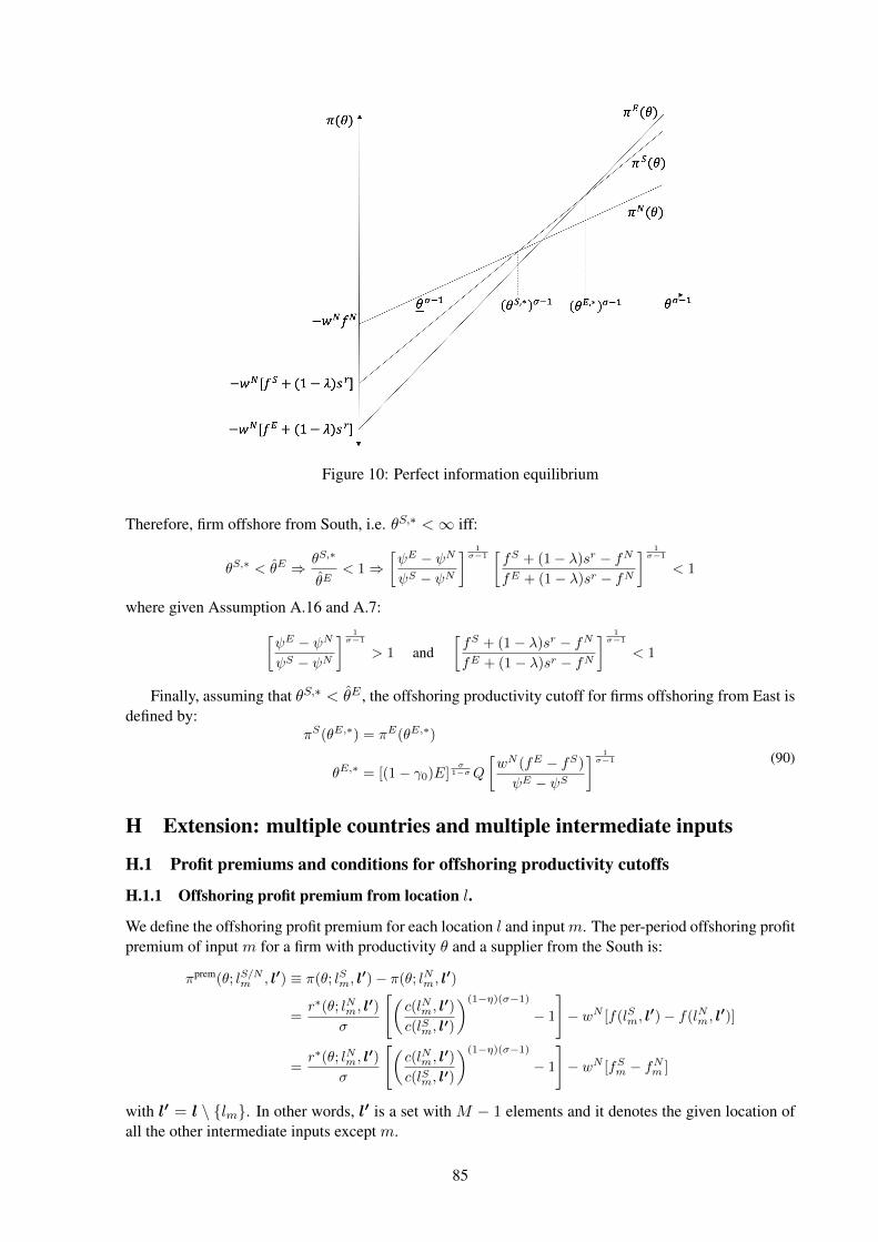
Figure 10: Perfect information equilibrium

Therefore, firm offshore from South, i.e. θS,∗ <∞ iff:

θS,∗ < θE ⇒ θS,∗

θE< 1⇒

[ψE − ψN

ψS − ψN

] 1σ−1

[fS + (1− λ)sr − fN

fE + (1− λ)sr − fN

] 1σ−1

< 1

where given Assumption A.16 and A.7:[ψE − ψN

ψS − ψN

] 1σ−1

> 1 and[fS + (1− λ)sr − fN

fE + (1− λ)sr − fN

] 1σ−1

< 1

Finally, assuming that θS,∗ < θE , the offshoring productivity cutoff for firms offshoring from East isdefined by:

πS(θE,∗) = πE(θE,∗)

θE,∗ = [(1− γ0)E]σ

1−σQ

[wN (fE − fS)

ψE − ψS

] 1σ−1 (90)

H Extension: multiple countries and multiple intermediate inputs

H.1 Profit premiums and conditions for offshoring productivity cutoffs

H.1.1 Offshoring profit premium from location l.

We define the offshoring profit premium for each location l and inputm. The per-period offshoring profitpremium of input m for a firm with productivity θ and a supplier from the South is:

πprem(θ; lS/Nm , l′) ≡ π(θ; lSm, l′)− π(θ; lNm, l

′)

=r∗(θ; lNm, l

′)

σ

[(c(lNm, l

′)

c(lSm, l′)

)(1−η)(σ−1)

− 1

]− wN [f(lSm, l

′)− f(lNm, l′)]

=r∗(θ; lNm, l

′)

σ

[(c(lNm, l

′)

c(lSm, l′)

)(1−η)(σ−1)

− 1

]− wN [fSm − fNm ]

with l′ = l \ {lm}. In other words, l′ is a set with M − 1 elements and it denotes the given location ofall the other intermediate inputs except m.

85

Equivalently, the per-period offshoring profit premium of input m for a firm with productivity θ anda supplier from the East is:

πprem(θ; lE/Nm , l′) ≡ π(θ; lEm, l′)− π(θ; lNm, l

′)

=r∗(θ; lNm, l

′)

σ

[(c(lNm, l

′)

c(lEm, l′)

)(1−η)(σ−1)

− 1

]− wN [f(lEm, l

′)− f(lNm, l′)]

=r∗(θ; lNm, l

′)

σ

[(c(lNm, l

′)

c(lEm, l′)

)(1−η)(σ−1)

− 1

]− wN [fEm − fNm ]

H.1.2 Conditions for offshoring productivity cutoffs

The condition for offshoring from South is defined by:

π(θ, lSm, l

′)− wN (1− λ) sr(lSm, l

′) ≥ π (θ, lNm, l′)− wN (1− λ)sr(lNm, l

′)The cutoff θSm is defined by the binding case of the condition above. Therefore:

π(θSm, l

Sm, l

′)− π (θSm, lNm, l′) = wN (1− λ)[sr(lSm, l

′)− sr (lNm, l′)]π(θSm, l

Sm, l

′)− π (θSm, lNm, l′) = wN (1− λ)sr,Sm

Solving for the productivity cutoff:

θSm = [(1− γ0)E]σ

1−σQ

wN[f(lSm, l

′)− f(lNm, l′) + (1− λ)sr,Sm

]ψ(lSm, l

′)− ψ(lNm, l′)

1

σ−1

⇒ θSm = [(1− γ0)E]σ

1−σQ

wN[fSm − fNm + (1− λ)sr,Sm

]ψ(lSm, l

′)− ψ(lNm, l′)

1

σ−1

Let’s temporary define θE,•m as:

π(θE,•m , lEm, l

′)− π (θE,•m , lNm, l′) = wN (1− λ)

[srm(lEm, l

′)− srm (lNm, l′)]π(θE,•m , lEm, l

′)− π (θE,•m , lNm, l′) = wN (1− λ)sr,Em

⇒ θE,•m = [(1− γ0)E]σ

1−σQ

wN[fEm − fNm + (1− λ)sr,Em

]ψ(lEm, l

′)− ψ(lNm, l′)

1

σ−1

Therefore, the offshoring productivity cutoff in South for input m is lower than in East when:

θSm

θE,•m

=

[ψ(lEm, l

′)− ψ(lNm, l′)


′)

] 1σ−1

[fSm + (1− λ)sr,Sm − fNmfEm + (1− λ)sr,Em − fNm

] 1σ−1

< 1

Assuming the condition from above holds. The productivity condition for offshoring firms from Eastin input m, i.e. θ ≥ θEm, is given by:

π(θ, lEm, l

′)− wN (1− λ) sr(lEm, l

′) ≥ π (θ, lSm, l′)− wN (1− λ) sr(lSm, l

′)Solving for the productivity cutoff in a similar way as before:

θEm = [(1− γ0)E]σ

1−σQ

wN[fEm − fSm + (1− λ)

(sr,Em − sr,Sm

)]ψ(lEm, l

′)− ψ(lSm, l′)

1

σ−1

86

H.2 Scenario 1: Small open economy

H.2.1 Market share of country N ’ firms in world market

The aggregate consumption index in the differentiated sector in the world market isQ =[∑N

N=1

[QN]α] 1

α ,

and the aggregate production of final-good producers from country N in is QN =[∫i∈IN [qN (i)]αdi

] 1α .

Therefore, the world market aggregate consumption index is:

Q =

[ N∑N=1

∫i∈IN

[qN (i)]αdi

] 1α

Dividing both, we have the market share of the country N in the world market economy:[QNjQj

]αj=

∫i∈INj

[qNj (i)]αjdi∑NN=1

∫i∈INj

[qNj (i)]αjdi⇒

QNjQj

=

∫i∈INj

[qNj (i)]αjdi∑NN=1

∫i∈INj

[qNj (i)]αjdi

1αj

H.3 Profit function: slope’s differences across locations for input m.


′) =ασ−1

σ(wN )η(1−σ)

[c(lSm, l

′)(1−η)(1−σ) − c(lNm, l′)(1−η)(1−σ)]

=ασ−1

σ(wN )η(1−σ)

M∏m′=1m′ 6=m

(ωm′

clm′m′

)ωm′ (1−η)(σ−1)

×

[(ωmcSm

)ωm(1−η)(σ−1)

−(ωmwN

)ωm(1−η)(σ−1)]

Equivalently,

ψ(lEm, l′)− ψ(lNm, l

′) =ασ−1

σ(wN )η(1−σ)

M∏m′=1m′ 6=m

(ωm′

clm′m′

)ωm′ (1−η)(σ−1)

×

[(ωmcEm

)ωm(1−η)(σ−1)

−(ωmwN

)ωm(1−η)(σ−1)]

and

ψ(lEm, l′)− ψ(lSm, l

′) =ασ−1

σ(wN )η(1−σ)

M∏m′=1m′ 6=m

(ωm′

clm′m′

)ωm′ (1−η)(σ−1)

×

[(ωmcEm

)ωm(1−η)(σ−1)

−(ωmcSm

)ωm(1−η)(σ−1)]

H.4 Learning

The maximum affordable fixed costs computed by the firms depend on the offshoring status of the leastproductive firm offshoring from East in the previous period.

The least productive firm sourcing from the East at the beginning of the period t is denoted as θEm,t.In the case that this firm previous sourcing location was a northern supplier, i.e. dSm,t−1(θ

Em,t) = 0, the

maximum affordable fixed cost for that firm in order to remain sourcing from East is given by:

πpremt (θEm,t; l

E/Nm , l′t) = πt(θ

Em,t; l

Em, l

′t)− πt(θEm,t; lNm, l′t) = 0

fEm,t ≡ fEm(θEm,t) =rt(θ; l

Nm, l

′t)

wNσ

[(c(lNm, l

′t)

c(lEm, l′t)

)(1−η)(σ−1)

− 1

]+ fNm

87

On the other hand, if the firm θEm,t previous sourcing location of inputmwas South, i.e. dSm,t−1(θEm,t) =

1, the maximum affordable fixed cost is define by the following condition:

πpremt (θEm,t; l

E/Sm , l′t) = πt(θ

Em,t; l

Em, l

′t)− πt(θEm,t; lSm, l′t) = 0

fEm,t ≡ fEm(θEm,t) =rt(θ; l

Nm, l

′t)

wNσ

[(c(lNm, l

′t)

c(lEm, l′t)

)(1−η)(σ−1)

−(c(lNm, l

′t)

c(lSm, l′t)

)(1−η)(σ−1)]

+ fSm

with

πpremt (θEm,t; l

E/Sm , l′t) = πt(θ

Em,t; l

Em, l

′t)− πt(θEm,t; lSm, l′t)

=rt(θ; l

Nm, l

′)

σ

[(c(lNm, l

′)

c(lEm, l′)

)(1−η)(σ−1)

−(c(lNm, l

′)

c(lSm, l′)

)(1−η)(σ−1)]− wN [fEm − fSm]

H.5 Convergence analysis: general equilibrium

We relax now the small economy assumption, and characterise the equilibrium path of the entire dif-ferentiated sector, considering that the firms modelled here represent the entire universe of firms in thatsector. In other words, it is possible to think this section as the case in which there is only one countryin North, or alternatively, a situation in which the informational externalities spreads perfectly to all thecountries N ∈ N.

The analysis can still be partially separated across inputs. However, there is a general equilibriumeffect through the price index P that links all the sourcing decisions in each period t. Thus, the decisionsare taken simultaneously and the solution can be characterised by finding the multidimensional fixedpoint of the system of equations.

This section builds on the results already obtained for the small economy in section 6.4.5, introducingthe modifications implied by the GE effects.

The analysis starts by solving the offshoring productivity cutoffs for each type of inputs, takingPt, Pt+1 and thus Qt, Qt+1 as given. Therefore, after the characterisation of the equilibrium path of eachtype of inputs, we show the general equilibrium sectoral dynamic path by characterising the fixed pointof the system of equations that defines the vector of offshoring productivity cutoffs in each period t.

A first effect easy to observe due to the general equilibrium competition effect, already present inthe simple model with one intermediate input, is that the market productivity cutoff increases over timeθt ↑ θ∗, as more firms explore their offshoring potential in the East.

Type I inputs’ set:={m :m ∈M ;wN < cSm;wN < cEm

}As before, no firm among the active

ones θ ≥ θt at any period t find it profitable to explore the offshoring potential from any foreign location.Formally, we have:

θS,initialm = θS,∗m →∞ ∀t

DEm,t(

¯θ;θt, θt+1

)< 0 ∀t

with ¯θ as the most productive firm in the market.


}The ex-

ploration of eastern institutions may still take place under the conditions shown in section 6.4.5. How-ever, additional dynamics emerge in relation to the offshoring productivity cutoff in the South, as a resultof the increasing competition that comes from the progressively decreasing price index.

The initial offshoring productivity cutoff in input m from South is given by:

θS,initialm =

[(1− γ0)E]σ

1−σQinitial[wN [fSm−fNm+(1−λ)sr,Sm ]


] 1σ−1

if ≤ ¯θ

∞ if > ¯θ

88

In the second case, the productivity cutoff is above the productivity level of the most productive firmin the market88, therefore θSm,t = θS,∗m → ∞ ∀t89. In the first case, however, the initial offshoringproductivity cutoff is smaller than the perfect information steady state condition, i.e. θS,initial

m < θS,∗m .Due to the initial lower competition in the market, the firms with productivity θ ∈ [θS,initial

m , θS,∗m ) find itprofitable to offshore m from South.

We know that the consumption price index is monotonically decreasing in the vector θt, and thus Qtincreases pari passu. Therefore, as more firms offshore any intermediate input m ∈ M , the decreasingprice index generates that the marginal firms sourcing m from the South must sequentially relocate theirsupply chain to the North. This reshoring strategy is a direct result of the increasing competition in thefinal goods market.

Formally, the offshoring productivity cutoff in South at the beginning of period t is given by:

θS,initialm ≤ θSm,t = [(1− γ0)E]

σ1−σQt

[wN

[fSm − fNm

]ψ(lSm, l

′)− ψ(lNm, l′)

] 1σ−1

The expected offshoring productivity cutoff of input m ∈ Type II in South, as a result of the overalloffshoring exploration in t, is denoted as:

θSm,t+1 = [(1− γ0)E]σ

1−σ Qt+1

[wN

[fSm − fNm

]ψ(lSm, l

′)− ψ(lNm, l′)

] 1σ−1

with Qt+1 = Q(θt+1). The offshoring productivity cutoffs in the expression above represents theexpected state of the system in t+ 1 for the respective inputs m ∈ Type II.


}We as-

sume that Assumption A.12 still holds. Thus, the offshoring productivity cutoff from East for m ∈ TypeIII in period t is given by:

θEm,t+1 =

[(1− γ0)E]σ

1−σ Qt+1

wN[Et(fEm|It)−fNm+sr,Em

(1−λ


)]ψ(lEm,l′t)−ψ(lNm,l′t)

1

σ−1


[(1− γ0)E]σ

1−σ Qt+1

wN[Et(fEm|It)−fSm+sr,Em

(1−λ


)]ψ(lEm,l

′)−ψ(lSm,l′)

1

σ−1


(91)with θEm,t+1 →∞ for any period t in which the productivity cutoff is larger than ¯θ.

Regarding the characterisation of the first entrants and the exploration sequence in inputs from East,it is still defined in an equivalent way as before, and Proposition 8 remains valid.

Competition effect and relocation of the supply chain. The initial offshoring productivity cutofffrom South for inputs m ∈ Type III are:

θS,initialm =

[(1− γ0)E]σ

1−σQinitial[wN [fSm−fNm+(1−λ)sr,Sm ]


] 1σ−1

< θS,∗m if ≤ ¯θ ∧ cSm < wN

∞ if > ¯θ ∨ cSm ≥ wN

88This does not take place if the productivity distribution G(θ) is unbounded on the right, i.e. if ¯θ →∞.89In general terms, θS,initial

m < θS,∗m for every m ∈ Type II. However, if the condition in the first line for an input m ∈ Type IIis larger than ¯θ, we observe from the initial conditions that input m is at its perfect information offshoring productivity cutofflevel, i.e. no firm offshores the input m from South.

89

The reduction in the price index, and the consequent increasing competition, pushes upwards theoffshoring productivity cutoff in South. Thence, the least productive firms initially offshoring from Ssequentially move towards domestic suppliers (reshoring)90.

The offshoring productivity cutoff from South at the beginning of period t is given by:

θSm,t =

[(1− γ0)E]σ

1−σQt

[wN [fSm−fNm ]


] 1σ−1

if < θEm,t

∞ if ≥ θEm,t

and the expected offshoring productivity cutoff from South, as a result of the expected overall offshoringexploration in t, is given by:

θSm,t+1 =

[(1− γ0)E]σ

1−σ Qt+1

[wN [fSm−fNm ]


] 1σ−1

if < θEm,t+1

∞ if ≥ θEm,t+1

Finally, a sequential relocation of offshoring firms from East takes place for the least relevant inputsand the least offshoring productive firms. The Proposition 8 shows that firms explore the offshoringpotential sequentially in inputs, starting from those with larger ψ(lEm, l

′) − ψ(lSm, l′) or ψ(lEm, l

′) −ψ(lNm, l

′), depending on the previous sourcing location of the input.However, as the competition effect intensifies, the least productive firms offshoring from East the

relatively less relevant inputs realise that they are not productive enough to keep offshoring from thatlocation. Therefore, they shift sequentially their supply chain in these inputs to their previous location.

90As Pt ↓ P ∗, and thus Qt ↑ Q∗, some inputs m with θS,initialm < ¯θ may be fully reshored if the conditions θSm,t > ¯θ and

θEm,t >¯θ hold simultaneously as t→∞.

90

Contents1 Introduction 1

2 The two-country model: North-South 42.1 Perfect information equilibrium . . . . . . . . . . . . . . . . . . . . . . . . . . . . . . . . . . . 52.2 The North-South global sourcing dynamic model with uncertainty . . . . . . . . . . . . . . . . . 6

2.2.1 Timing of events . . . . . . . . . . . . . . . . . . . . . . . . . . . . . . . . . . . . . . . 72.2.2 Initial conditions: non-tradable intermediate inputs (n.t.i.) . . . . . . . . . . . . . . . . . 72.2.3 Dynamic model with uncertainty: tradable intermediate inputs . . . . . . . . . . . . . . . 9

3 Empirics: Two-country model 143.1 Data description and sample selection . . . . . . . . . . . . . . . . . . . . . . . . . . . . . . . . 143.2 Conditional probability model . . . . . . . . . . . . . . . . . . . . . . . . . . . . . . . . . . . . 153.3 Transition (or survival) analysis . . . . . . . . . . . . . . . . . . . . . . . . . . . . . . . . . . . 16

4 The multi-country model 174.1 Multi-country model with symmetric wages . . . . . . . . . . . . . . . . . . . . . . . . . . . . . 18

4.1.1 Firms’ offshoring decision . . . . . . . . . . . . . . . . . . . . . . . . . . . . . . . . . . 184.1.2 Case A: Equilibria with symmetric initial beliefs . . . . . . . . . . . . . . . . . . . . . . 194.1.3 Equilibria with asymmetric initial beliefs . . . . . . . . . . . . . . . . . . . . . . . . . . 22

4.2 Final consideration on the multi-country model and policy implications. . . . . . . . . . . . . . . 25

5 Empirics: Multi-country model with one intermediate input 265.1 Conditional probability model . . . . . . . . . . . . . . . . . . . . . . . . . . . . . . . . . . . . 275.2 Survival (or transition) analysis . . . . . . . . . . . . . . . . . . . . . . . . . . . . . . . . . . . . 305.3 IV model: Multi-country with one intermediate input . . . . . . . . . . . . . . . . . . . . . . . . 31

6 Extension: Multiple intermediate inputs 336.1 Firms’ profit maximisation problem . . . . . . . . . . . . . . . . . . . . . . . . . . . . . . . . . 33

6.1.1 Cost minimisation and unit cost function . . . . . . . . . . . . . . . . . . . . . . . . . . 346.1.2 Profit maximisation: optimal level of inputs . . . . . . . . . . . . . . . . . . . . . . . . . 346.1.3 Profit maximisation: optimal location of intermediate inputs suppliers . . . . . . . . . . . 35

6.2 Offshoring (market) research costs: sunk cost per-input and location . . . . . . . . . . . . . . . . 356.3 Perfect information equilibrium . . . . . . . . . . . . . . . . . . . . . . . . . . . . . . . . . . . 35

6.3.1 Equilibrium offshoring productivity cutoffs . . . . . . . . . . . . . . . . . . . . . . . . . 356.3.2 Import shares: extensive margin . . . . . . . . . . . . . . . . . . . . . . . . . . . . . . . 36

6.4 Uncertainty - Scenario 1: Institutional reform in East . . . . . . . . . . . . . . . . . . . . . . . . 366.4.1 Multiple northern countries: Small economy N assumption. . . . . . . . . . . . . . . . . 376.4.2 Initial conditions: . . . . . . . . . . . . . . . . . . . . . . . . . . . . . . . . . . . . . . 376.4.3 Prior uncertainty and learning . . . . . . . . . . . . . . . . . . . . . . . . . . . . . . . . 376.4.4 Firms’ offshoring decision . . . . . . . . . . . . . . . . . . . . . . . . . . . . . . . . . . 396.4.5 Convergence analysis: small economy N . . . . . . . . . . . . . . . . . . . . . . . . . . 40

6.5 Uncertainty - Scenario 2: Simultaneous institutional reforms in East and South . . . . . . . . . . 426.5.1 Initial conditions . . . . . . . . . . . . . . . . . . . . . . . . . . . . . . . . . . . . . . . 426.5.2 Prior uncertainty and learning . . . . . . . . . . . . . . . . . . . . . . . . . . . . . . . . 436.5.3 Firms’ offshoring decision . . . . . . . . . . . . . . . . . . . . . . . . . . . . . . . . . . 446.5.4 Convergence analysis: Multiple equilibria. Small economy N . . . . . . . . . . . . . . . 46

7 Empirics: Two-country model with multiple intermediate inputs 507.1 Conditional probability model . . . . . . . . . . . . . . . . . . . . . . . . . . . . . . . . . . . . 50

7.1.1 Survival (or transition) analysis . . . . . . . . . . . . . . . . . . . . . . . . . . . . . . . 52

8 Conclusions, extensions and next steps 54

A Perfect information model 58A.1 Consumer’s problem . . . . . . . . . . . . . . . . . . . . . . . . . . . . . . . . . . . . . . . . . 58A.2 Producers’ problem . . . . . . . . . . . . . . . . . . . . . . . . . . . . . . . . . . . . . . . . . . 58

91

B Initial conditions: Non-tradable intermediate inputs (n.t.i.) 59B.1 Sectoral price index . . . . . . . . . . . . . . . . . . . . . . . . . . . . . . . . . . . . . . . . . . 60B.2 Sectoral aggregate consumption . . . . . . . . . . . . . . . . . . . . . . . . . . . . . . . . . . . 60B.3 Zero Cutoff Profit Condition (ZCPC) . . . . . . . . . . . . . . . . . . . . . . . . . . . . . . . . . 60B.4 Free Entry Condition (FEC) . . . . . . . . . . . . . . . . . . . . . . . . . . . . . . . . . . . . . 61B.5 Equilibrium: number of firms . . . . . . . . . . . . . . . . . . . . . . . . . . . . . . . . . . . . . 61

C Perfect information: tradable intermediate inputs 62C.1 Price index in sector j . . . . . . . . . . . . . . . . . . . . . . . . . . . . . . . . . . . . . . . . . 63C.2 Aggregate consumption in sector j . . . . . . . . . . . . . . . . . . . . . . . . . . . . . . . . . . 65C.3 Firm entry and exit . . . . . . . . . . . . . . . . . . . . . . . . . . . . . . . . . . . . . . . . . . 65

C.3.1 Zero Cutoff Profit Condition (ZCPC) . . . . . . . . . . . . . . . . . . . . . . . . . . . . 65C.3.2 Free Entry Condition (FEC) . . . . . . . . . . . . . . . . . . . . . . . . . . . . . . . . . 66C.3.3 Sectoral equilibrium. Number of firms. . . . . . . . . . . . . . . . . . . . . . . . . . . . 66

C.4 Offshoring productivity cutoff . . . . . . . . . . . . . . . . . . . . . . . . . . . . . . . . . . . . 66

D Uncertainty - dynamic model: tradable intermediate inputs. 67D.1 Proofs regarding Bayesian learning mechanism . . . . . . . . . . . . . . . . . . . . . . . . . . . 67D.2 Proof of the OSLA rule as optimal policy . . . . . . . . . . . . . . . . . . . . . . . . . . . . . . 68D.3 Derivation of the trade-off function . . . . . . . . . . . . . . . . . . . . . . . . . . . . . . . . . . 71D.4 Proof of Proposition 1 . . . . . . . . . . . . . . . . . . . . . . . . . . . . . . . . . . . . . . . . . 72D.5 Proof of Proposition 2 . . . . . . . . . . . . . . . . . . . . . . . . . . . . . . . . . . . . . . . . . 73D.6 Proofs of Propositions 3, 4 (long-run properties) . . . . . . . . . . . . . . . . . . . . . . . . . . . 73

E Empirical model 74E.1 Two-country model with one intermediate input . . . . . . . . . . . . . . . . . . . . . . . . . . . 74E.2 Multi-country model with one intermediate input . . . . . . . . . . . . . . . . . . . . . . . . . . 75

E.2.1 IV approach: multi-country model with one intermediate input . . . . . . . . . . . . . . . 78E.3 Two-country model with multiple intermediate inputs . . . . . . . . . . . . . . . . . . . . . . . . 83

F Uncertainty - multicountry model. 84

G Extension: multiple countries with heterogeneous wages and institutional fundamentals 84

H Extension: multiple countries and multiple intermediate inputs 85H.1 Profit premiums and conditions for offshoring productivity cutoffs . . . . . . . . . . . . . . . . . 85

H.1.1 Offshoring profit premium from location l. . . . . . . . . . . . . . . . . . . . . . . . . . 85H.1.2 Conditions for offshoring productivity cutoffs . . . . . . . . . . . . . . . . . . . . . . . . 86

H.2 Scenario 1: Small open economy . . . . . . . . . . . . . . . . . . . . . . . . . . . . . . . . . . . 87H.2.1 Market share of country N ’ firms in world market . . . . . . . . . . . . . . . . . . . . . 87

H.3 Profit function: slope’s differences across locations for input m. . . . . . . . . . . . . . . . . . . 87H.4 Learning . . . . . . . . . . . . . . . . . . . . . . . . . . . . . . . . . . . . . . . . . . . . . . . . 87H.5 Convergence analysis: general equilibrium . . . . . . . . . . . . . . . . . . . . . . . . . . . . . . 88

92

uncertainty in global sourcing learning, sequential

Documents