Slide 1 of 21

Uncertainty Quantification in an IGCC Process Using Polynomial Chaos Expansions

Kenneth Hu

Bo Gong, Adekunle Adeyemo

Greg McRaeDepartment of Chemical Engineering, MIT

AIChE Annual Meeting, NashvilleNovember 12, 2009

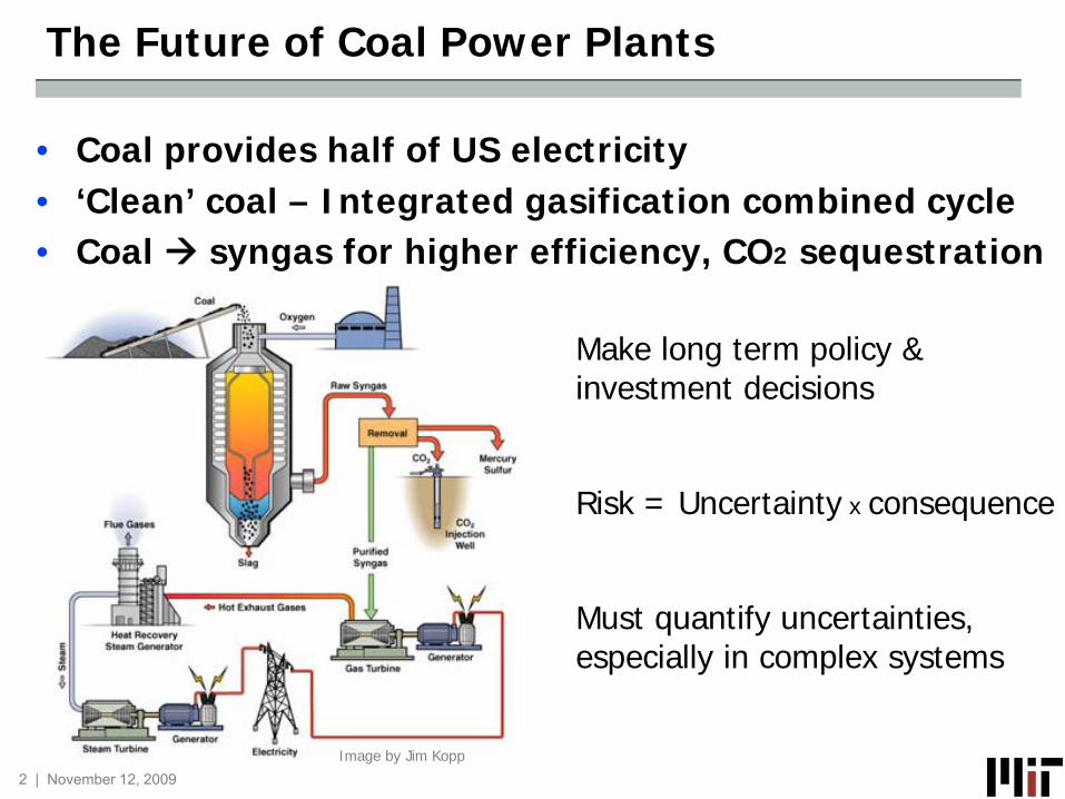
• Coal provides half of US electricity• ‘Clean’ coal – Integrated gasification combined cycle• Coal syngas for higher efficiency, CO2 sequestration

The Future of Coal Power Plants

2 | November 12, 2009

Risk = Uncertainty x consequence

Make long term policy & investment decisions

Must quantify uncertainties, especially in complex systems

Image by Jim Kopp

• Uncertainty Quantification in Chemical Systems• Tools for Uncertainty Quantification

• Polynomial Chaos Expansions• Illustrative Examples – Batch reactor• Coal Conversion Study – Apply to process design• Future Applications

Outline

3 | November 12, 2009

Key Point: The way to get orders of magnitude reduction in solution time is to change the problem representation – treat uncertainty at the beginning, not at the end.

Not all inputs are Gaussian!

Gaussian inputs Gaussian output

Uncertainty Quantification in Chemical Systems

4 | November 12, 2009

• Characterize the input uncertainty• What impact do uncertain inputs have on the outputs?

PDF = probability density function

Process Model

Uncertain Inputs

Uncertain Output1pθ

nθ

Independent Variables

1θ

( ) ( )1, ˆ,ny fω θ θ= x…

ˆ=x x

npθ

yp

y

• Current Methods – limitations• Perturbation Method – local approximation• Moment Methods – linearized systems• Monte Carlo – expensive

• Desired properties of uncertainty methods• Accurate• Computationally efficient• Decompose output uncertainty ~ Global Sensitivities• Apply to nonlinear, black box models• Non Gaussian inputs• Approximate the full output PDF

What is the Goal of Uncertainty Quantification?

5 | November 12, 2009

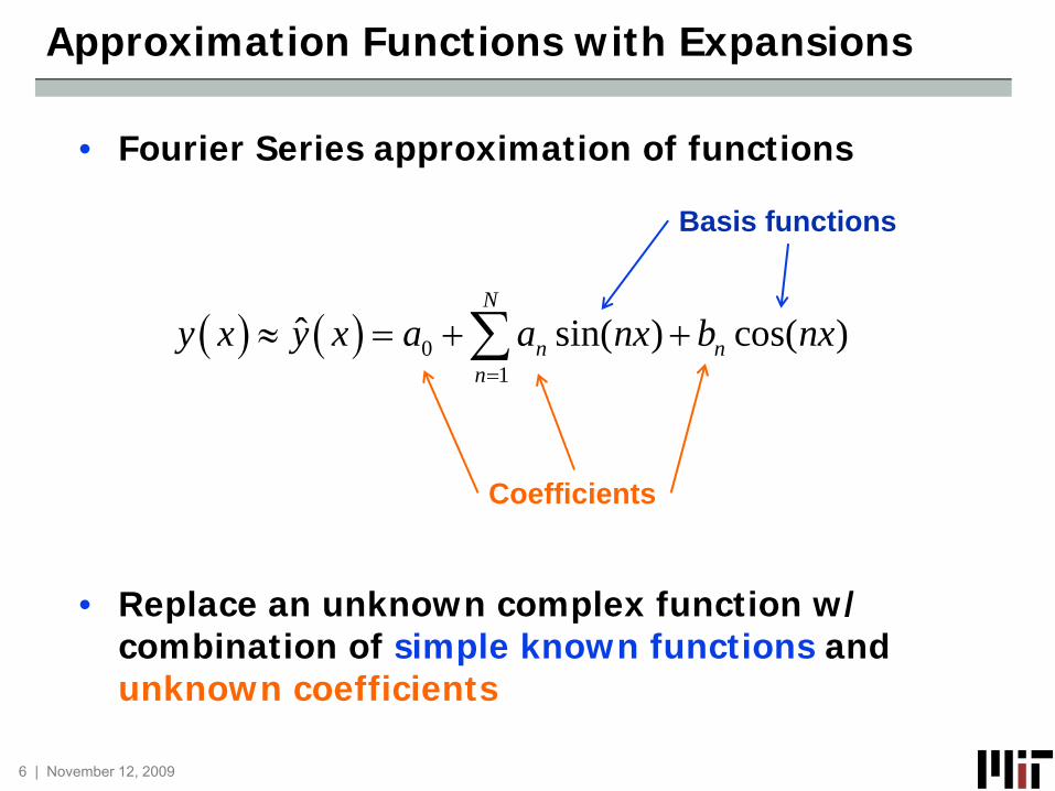
• Fourier Series approximation of functions

• Replace an unknown complex function w/ combination of simple known functions and unknown coefficients

Approximation Functions with Expansions

6 | November 12, 2009

( ) ( ) 01

ˆ sin( ) cos( )N

n nn

y x y x a a nx b nx=

≈ = + +∑

Basis functions

Coefficients

• Direct Representation of Random Variables (RV)

• How to choose the best Basis Random Variables and functionals?

Approximating a Random Variable

7 | November 12, 2009

( ) ( ) ( )0

ˆJ

j jj

Y Y yω ω=

≈ = Ψ∑ ξ

Basis RVs

Functionals of the Basis RVsCoefficients

Recall desired goals:1. Decompose output uncertainties

How – ensure inputs are independent

Representation – Orthogonal Basis Random Variables

2. Efficient computation of PDF/ statistics

How – Solve multidimensional integrals

ex:

Representation – Orthogonal polynomial functionals

ex:

Choosing the Basis and Functionals

8 | November 12, 2009

( ) ( )1

1

1 1 1n

n

n n nE Y dY fξ ξξ ξ

ξ ξ ξ ξ ξ ξ=⎡ ⎤⎣ ⎦ ∫ ∫ …… …… …

( ) ( )1 11

i

i

in i

n

i

f dE Y Y ξξ

ξ ξ ξ ξ=

⎡ ⎤⎢ ⎥⎢ ⎥⎣ ⎦

=⎡ ⎤⎣ ⎦ ∏ ∫…

Expansion of a Known Random Variable

9 | November 12, 2009

( ) ( ) ( ) ( )2 3 4 20 1 2 3 41 3 6 3X x x x x xω ξ ξ ξ ξ ξ ξ≈ + + − + − + − +

3.080-1.5270.392

-0.05970.0117

⎡ ⎤⎢ ⎥⎢ ⎥⎢ ⎥⎢ ⎥⎢ ⎥⎢ ⎥⎣ ⎦

=x

Gaussian Basis RV Hermite orthogonal polynomials( )~ 0,1Nξ

Choose a Basis RV

( )12~ logn 1,X

Specify

( ) ( ) ( )0

ˆk

K

kk

X xX ω ω=

≈ = Ψ∑ ξ

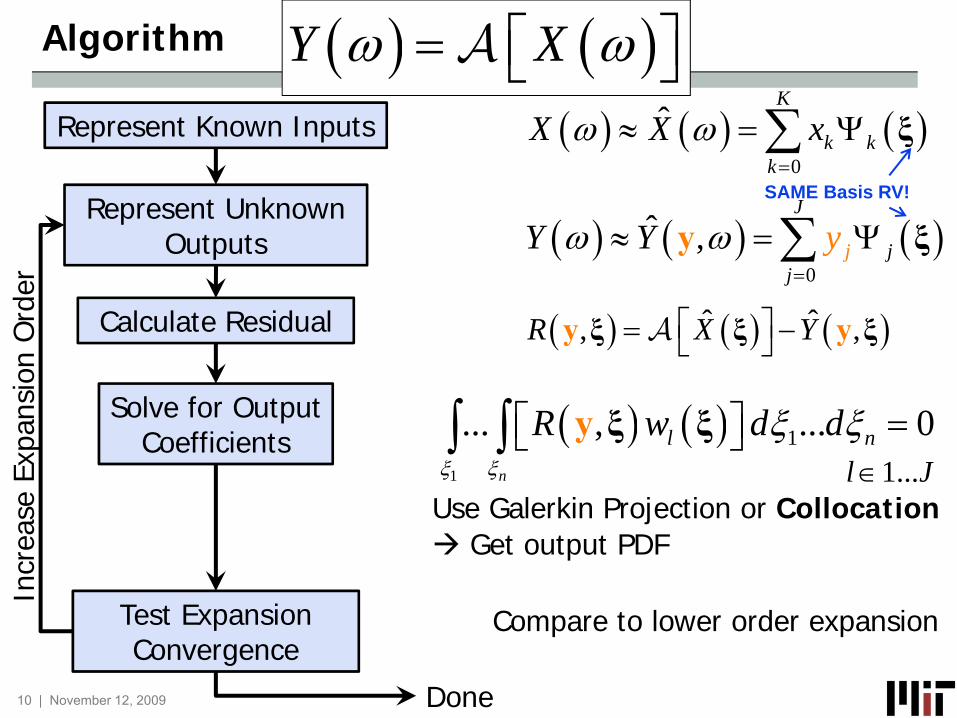
Algorithm

10 | November 12, 2009

( ) ( )Y Xω ω= ⎡ ⎤⎣ ⎦A

( ) ( ) ( )0

ˆ , j

J

jj

yY Yω ω=

≈ = Ψ∑ ξySAME Basis RV!

( ) ( ) ( )0

ˆk

K

kk

X xX ω ω=

≈ = Ψ∑ ξ

( ) ( ) ( )ˆ ˆ, ,R X Y⎡ ⎤ −= ⎣ ⎦ξ ξ ξy yA

Represent Unknown Outputs

Represent Known Inputs

Solve for OutputCoefficients

Test Expansion Convergence

Calculate Residual

( ) ( )1

1... , ... 0n

l nR w d dξ ξ

ξ ξ =⎡ ⎤⎣ ⎦∫ ∫ ξ ξy

Use Galerkin Projection or Collocation

Compare to lower order expansion

Incr

ease

Exp

ansi

on O

rder

Done

1...l J∈

Get output PDF

UQ Example – Batch Reactor

11 | November 12, 2009

( ) ( ) ( )( ), expY t X X tω ω ω= = −⎡ ⎤⎣ ⎦A 120fix t =

2 model evaluations 5 model evaluations

( )dY X Ydt

ω= −Uncertain kinetic parameter

( )12~logn 1,X( )0 1Y t = =

Efficient Quantification of Uncertainty

12 | November 12, 2009

• Uncertainty quantification adds a crucial dimension to the output

• Polynomial Chaos Expansions ‘Probability response surface’

Mean parameter value cannot accurately predict the outcomes

( )k E X ω= ⎡ ⎤⎣ ⎦

t=0.01

t=0.25

t=1

• Recap• Widely applicable tool for uncertainty

quantification• Orders of magnitude faster than Monte Carlo• Easily identify significant input uncertainties

• Assumptions/ Issues• Assume the approximate functional form of

the output density• Requires well behaved models• Uses concepts from numerical quadrature• Convergence rate

Polynomial Chaos Expansions – Summary

13 | November 12, 2009

• Integrated gasification combined cycle modeled in ASPEN Plus

• Quantify uncertainties• Identify parameters that require more study• Assess impact on design

Evaluating competing clean coal technologies

14 | November 12, 2009

Characterize Uncertain Input Parameters

15 | November 12, 2009

# Unit Parameter Distribution Mean Var Range σ/μ1 Moisture Normal 11.12 0.56 0.0672 Ash Normal 10.91 0.55 0.0683 Carbon Normal 71.72 3.59 0.0264 Hydrogen Normal 5.06 0.25 0.0995 Nitrogen Normal 1.41 0.0705 0.1886 Sulfur Normal 2.82 0.14 0.1337 Oxygen8 radiant temperature Uniform 593 133.33 40 0.0199 quench temperature Uniform 210 133.33 40 0.05510 overall carbon conversion Triangular 0.980 0.16 0.03 0.4011 expander η Triangular 0.800 0.10 0.1 0.3912 air compressor η Triangular 0.850 0.11 0.1 0.3913 gas turbine isentrop η Triangular 0.897 0.13 0.046 0.4014 gas turbine mech η Triangular 0.985 0.16 0.02 0.4115 HP-Turbine η Triangular 0.875 0.12 0.05 0.4016 MP-Turbine η Triangular 0.875 0.12 0.05 0.4017 IP-Turbine η Triangular 0.895 0.13 0.03 0.4018 NP-Turbine η Triangular 0.895 0.13 0.03 0.4019 LP-Turbine η Triangular 0.89 0.13 0.04 0.4020 air compressor η Triangular 0.804 0.10 0.072 0.3921 O2 booster η Triangular 0.735 0.08 0.13 0.3822 N2 compressor η Triangular 0.801 0.10 0.078 0.3923 LP compressor η Triangular 0.850 0.11 0.1 0.3924 MP compressor η Triangular 0.850 0.11 0.1 0.3925 HP compressor η Triangular 0.850 0.11 0.1 0.3926 CO2 pump η Triangular 0.750 0.08 0.1 0.38

Air Separation 

CO2 Compression

constrained by other components

Feedstock

Gasification

Gas turbine

Steam turbine

Coal Composition Parameters

mean

range

uniform/triangle PDFs

21 Parameters

Significant uncertainties

Non Gaussian Distributions

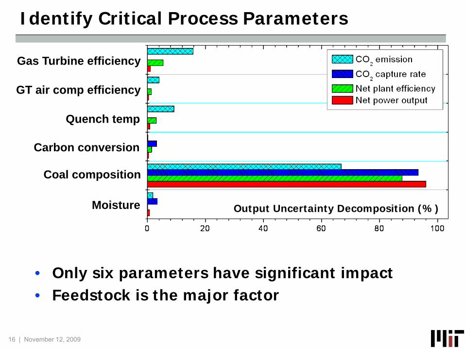
Moisture

Coal composition

Carbon conversion

Quench temp

GT air comp efficiency

Gas Turbine efficiency

Identify Critical Process Parameters

16 | November 12, 2009

• Only six parameters have significant impact• Feedstock is the major factor

Output Uncertainty Decomposition (%)

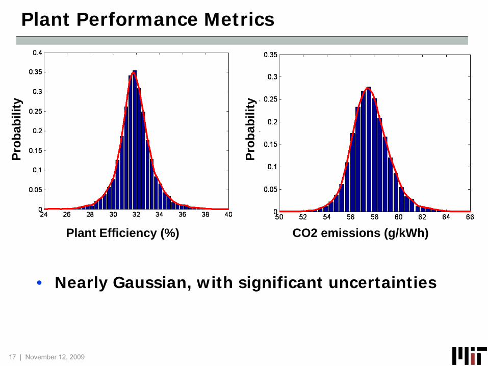
Plant Performance Metrics

17 | November 12, 2009

Plant Efficiency (%) CO2 emissions (g/kWh)

Prob

abili

ty

Prob

abili

ty

• Nearly Gaussian, with significant uncertainties

• Model is roughly linear in the significant parameter (Coal composition)

• Significant uncertainty in the outputs warrants further study of coal composition, matching of process conditions to coal source.

• Efficiency – 48 model evaluations, ~O(2) fewer than Monte Carlo

• Future work – integrate rigorous uncertainty quantification with process design

Results

18 | November 12, 2009

• Current uses• Computational Fluid Dynamics• Combustion• Subsurface flow

• Potential Chemical Engineering areas• Process Design• Experimental Design• Economic Analysis• Model Predictive Control• Anything related to Stochastic Optimization

Application Areas

19 | November 12, 2009

• Eni S.p.A.• BP

• McRae Group

Acknowledgements

20 | November 12, 2009

1. Wiener, N. (1938). "The Homogeneous Chaos." American Journal of Mathematics 60(4): 897-936.

2. Ghanem, R. and P. Spanos (1991). Stochastic Finite Elements: A Spectral Approach, Springer-Verlag.

3. M. A. Tatang, W. Pan, R. G. Prinn, and G. J. McRae. An Efficient Method for Parametric Uncertainty Analysis of Numerical Geophysical Models. Journal of Geophysical Research, 102 (1997), pp. 21916- 21924.

4. Xiu, D. (2009). "Fast numerical methods for stochastic computations: A review." Commun. Comput. Phys. 5(2-4): 242 272.

5. Cost and Performance Baseline for Fossil Energy Plant, Vol. 1, DOE/NETL – 2007/1281, (2007).

References

21 | November 12, 2009

Ken HuPhD CandidateDepartment of Chemical EngineeringMassachusetts Institute of Technologykthu@mit.edu

Contact Information