Uncertainty Quantification of Cooling Load Calculation

Da Lin, Dazhou Zhao Huadian Electric Power Research Institute Co., LTD, Hangzhou, China

E-mail: da-lin@chder.com, dazhou-zhao@ chder.com

Keywords:uncertainty quantification; cooling load; Monte Carlo simulation

Abstract: Cooling load calculation is commonly implemented with building energy simulation software among HVAC industry. While those software have limited ability to handle large amount of uncertain input data. Since they can only accept deterministic or scenario input data. In this paper, a new model is proposed to calculate the cooling load. The uncertainty of input data is considered and Monte Carlo simulation is used to calculate the building cooling load.

1. Introduction

Cooling load calculation is basis of HVAC system design, as HVAC system equipment selection is mainly depend on accurate quantification of building cooling load. Energy model and reliable input parameter are two important factors affect the accuracy of the cooling load prediction. Nowadays the energy model in most of the commercial software such as EnergyPlus, DeST and DOE-2 has matured over the past decades [1]. All those software use constants input parameter, such as occupants’ density, equipment heat gain or even weather data. But the uncertainty arises from those parameters is inevitable. For early design stage, because lacking knowledge about feature of building and operation schedule. Large number of parameters cannot be determined. On the other hand, the uncertainty behind some parameters are hardly to eliminate even under later design stage, since detailed measurement of those parameter is time consuming and costly. Machine learning or data mining have been implemented to predict the uncertainty input parameters or even to predict the total building cooling load. Limitation of this method is large number of history data required.

In this paper, a mathematical model for uncertainty cooling load calculation has been developed. The probability distributions of uncertainty parameters have been quantified. Finally, a real case cooling load has been calculated using uncertainty method.

2. Model

2.1 Model Overview

The cooling load calculation model is implemented with Monte Carlo simulation to quantify the uncertainty. Input parameter can be classified as two categories: deterministic parameter, uncertain parameter. The value of deterministic parameter and probability distribution of uncertain parameter would be varied as change of scenario. Monte Carlo simulations sample from a probability distribution for each parameter to produce enough possible outcomes. Finally, the cooling load

2018 2nd International Conference on Computer Science and Intelligent Communication (CSIC 2018)

Published by CSP © 2018 the Authors 40

probability distribution can be plotted. The whole process has been calculated by Matlab code. The detailed mathematical model is explained in the following two sections.

2.2 Solar Radiation Model

In this section, a solar radiation model is developed mainly based on clear sky model and Liu, Jordan deduction [2]. Solar gain is an important factor effecting the building cooling load. The variation of solar gain would significantly alter the building cooling load. So, an accurate solar radiation model would be essential for building cooling load calculation.

Solar radiation can be divided into three components: beam irradiation, diffused radiation, and reflected radiation. Normally any exterior surfaces of building can be categorized as two areas: sunlit area, shading area. Sunlit area will calculate total three components. Shading area will calculate last two components, since there is no beam irradiation on shading surface. For simplicity the reflected radiation is not taken into consideration. Therefore, the total insolation intensity on the titled surface would be calculated through Eq. (1)-(7). Where the solar constant 𝐼𝐼𝑆𝑆𝑆𝑆 = 1367𝑊𝑊/𝑚𝑚2. τ𝑏𝑏 is beam transmittance which change with variation of time and location. In this paper, τ𝑏𝑏 is 0.620 for time 12:00 [3].

It = IbRb + IdRd#(1) Ib = 𝐼𝐼0ℎτ𝑏𝑏#(2)

Id = 𝐼𝐼0ℎτ𝑑𝑑#(3)

τ𝑑𝑑 = 0.271 − 0.294τ𝑏𝑏#(4)

Rb =cos 𝜃𝜃𝑖𝑖cos 𝜃𝜃𝑧𝑧

#(5)

Rd =1 + cos𝛽𝛽

2#(6)

𝐼𝐼0ℎ = 𝐼𝐼𝑆𝑆𝑆𝑆 �1 + 0.034 cos �2𝜋𝜋𝑛𝑛

365.25�� cos 𝜃𝜃𝑧𝑧 #(7)

Detailed solar angle calculation is based on the following assumption: n = 1 on the 1st January; Vernal equinox day is 20th March, n = 79, δ = 0; Summer Solstice day is 21st June, n = 172, δ = 23.45; Autumnal Equinox day is 23rd September, n = 266, δ = 0; Winter Solstice day is 21st December, n = 355, δ = -23.45. The solar angle is calculated through Eq. (8)-(11).

cos 𝜃𝜃𝑖𝑖 = sin δ sinΦ cos𝛽𝛽 + sin δ cosΦ sin𝛽𝛽 cos𝐴𝐴𝑍𝑍𝑆𝑆+ cos δ cosΦ cos𝛽𝛽 cos𝜔𝜔

− cos δ sinΦ sin𝛽𝛽 cos𝐴𝐴𝑍𝑍𝑆𝑆 cos𝜔𝜔− cos δ sin𝛽𝛽 sin𝐴𝐴𝑍𝑍𝑆𝑆 sin𝜔𝜔 #(8)

δ = 23.45𝜋𝜋

180sin �2𝜋𝜋 �

284 + 𝑛𝑛365.25 �

�#(9)

For simplicity, only vertical walls and horizontal roofs are taken into consideration. For vertical wall, β= π/2, then there is Equation (10).

cos𝜃𝜃𝑖𝑖 = sin δ cosΦ cos𝐴𝐴𝑍𝑍𝑆𝑆 − cos δ sinΦ cos𝐴𝐴𝑍𝑍𝑆𝑆 cos𝜔𝜔− cos δ sin𝐴𝐴𝑍𝑍𝑆𝑆 sin𝜔𝜔 #(10)

For horizontal roof, β=0, then there is Equation (11).

41

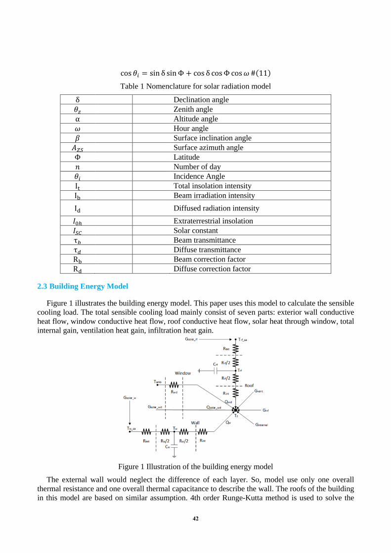
cos 𝜃𝜃𝑖𝑖 = sin δ sinΦ + cos δ cosΦ cos𝜔𝜔 #(11) Table 1 Nomenclature for solar radiation model

δ Declination angle 𝜃𝜃𝑧𝑧 Zenith angle α Altitude angle 𝜔𝜔 Hour angle 𝛽𝛽 Surface inclination angle 𝐴𝐴𝑍𝑍𝑆𝑆 Surface azimuth angle Φ Latitude 𝑛𝑛 Number of day 𝜃𝜃𝑖𝑖 Incidence Angle It Total insolation intensity Ib Beam irradiation intensity Id Diffused radiation intensity 𝐼𝐼0ℎ Extraterrestrial insolation 𝐼𝐼𝑆𝑆𝑆𝑆 Solar constant τ𝑏𝑏 Beam transmittance τ𝑑𝑑 Diffuse transmittance Rb Beam correction factor Rd Diffuse correction factor

2.3 Building Energy Model

Figure 1 illustrates the building energy model. This paper uses this model to calculate the sensible cooling load. The total sensible cooling load mainly consist of seven parts: exterior wall conductive heat flow, window conductive heat flow, roof conductive heat flow, solar heat through window, total internal gain, ventilation heat gain, infiltration heat gain.

Figure 1 Illustration of the building energy model

The external wall would neglect the difference of each layer. So, model use only one overall thermal resistance and one overall thermal capacitance to describe the wall. The roofs of the building in this model are based on similar assumption. 4th order Runge-Kutta method is used to solve the

42

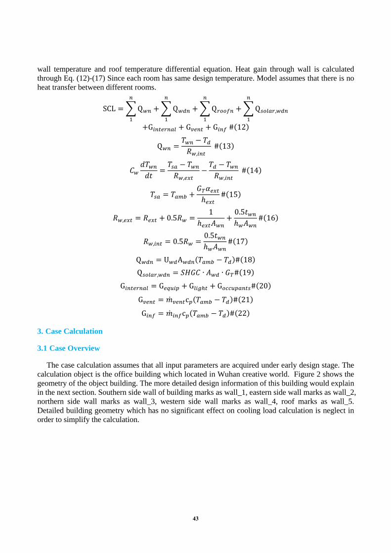
wall temperature and roof temperature differential equation. Heat gain through wall is calculated through Eq. (12)-(17) Since each room has same design temperature. Model assumes that there is no heat transfer between different rooms.

SCL = �Q𝑤𝑤𝑛𝑛

𝑛𝑛

1

+ �Q𝑤𝑤𝑑𝑑𝑛𝑛

𝑛𝑛

1

+ �Q𝑟𝑟𝑟𝑟𝑟𝑟𝑟𝑟𝑛𝑛

𝑛𝑛

1

+ �Q𝑠𝑠𝑟𝑟𝑠𝑠𝑠𝑠𝑟𝑟,𝑤𝑤𝑑𝑑𝑛𝑛

𝑛𝑛

1+G𝑖𝑖𝑛𝑛𝑖𝑖𝑖𝑖𝑟𝑟𝑛𝑛𝑠𝑠𝑠𝑠 + G𝑣𝑣𝑖𝑖𝑛𝑛𝑖𝑖 + G𝑖𝑖𝑛𝑛𝑟𝑟 #(12)

Q𝑤𝑤𝑛𝑛 =𝑇𝑇𝑤𝑤𝑛𝑛 − 𝑇𝑇𝑑𝑑𝑅𝑅𝑤𝑤,𝑖𝑖𝑛𝑛𝑖𝑖

#(13)

𝐶𝐶𝑤𝑤𝑑𝑑𝑇𝑇𝑤𝑤𝑛𝑛𝑑𝑑𝑑𝑑

=𝑇𝑇𝑠𝑠𝑠𝑠 − 𝑇𝑇𝑤𝑤𝑛𝑛𝑅𝑅𝑤𝑤,𝑖𝑖𝑒𝑒𝑖𝑖

−𝑇𝑇𝑑𝑑 − 𝑇𝑇𝑤𝑤𝑛𝑛𝑅𝑅𝑤𝑤,𝑖𝑖𝑛𝑛𝑖𝑖

#(14)

𝑇𝑇𝑠𝑠𝑠𝑠 = 𝑇𝑇𝑠𝑠𝑎𝑎𝑏𝑏 +𝐺𝐺𝑇𝑇𝛼𝛼𝑖𝑖𝑒𝑒𝑖𝑖ℎ𝑖𝑖𝑒𝑒𝑖𝑖

#(15)

𝑅𝑅𝑤𝑤,𝑖𝑖𝑒𝑒𝑖𝑖 = 𝑅𝑅𝑖𝑖𝑒𝑒𝑖𝑖 + 0.5𝑅𝑅𝑤𝑤 =1

ℎ𝑖𝑖𝑒𝑒𝑖𝑖𝐴𝐴𝑤𝑤𝑛𝑛+

0.5𝑑𝑑𝑤𝑤𝑛𝑛ℎ𝑤𝑤𝐴𝐴𝑤𝑤𝑛𝑛

#(16)

𝑅𝑅𝑤𝑤,𝑖𝑖𝑛𝑛𝑖𝑖 = 0.5𝑅𝑅𝑤𝑤 =0.5𝑑𝑑𝑤𝑤𝑛𝑛ℎ𝑤𝑤𝐴𝐴𝑤𝑤𝑛𝑛

#(17)

Q𝑤𝑤𝑑𝑑𝑛𝑛 = U𝑤𝑤𝑑𝑑A𝑤𝑤𝑑𝑑𝑛𝑛(𝑇𝑇𝑠𝑠𝑎𝑎𝑏𝑏 − 𝑇𝑇𝑑𝑑)#(18) Q𝑠𝑠𝑟𝑟𝑠𝑠𝑠𝑠𝑟𝑟,𝑤𝑤𝑑𝑑𝑛𝑛 = 𝑆𝑆𝑆𝑆𝐺𝐺𝐶𝐶 ∙ 𝐴𝐴𝑤𝑤𝑑𝑑 ∙ 𝐺𝐺𝑇𝑇#(19)

G𝑖𝑖𝑛𝑛𝑖𝑖𝑖𝑖𝑟𝑟𝑛𝑛𝑠𝑠𝑠𝑠 = G𝑖𝑖𝑒𝑒𝑒𝑒𝑖𝑖𝑒𝑒 + G𝑠𝑠𝑖𝑖𝑙𝑙ℎ𝑖𝑖 + G𝑟𝑟𝑜𝑜𝑜𝑜𝑒𝑒𝑒𝑒𝑠𝑠𝑛𝑛𝑖𝑖𝑠𝑠#(20)

G𝑣𝑣𝑖𝑖𝑛𝑛𝑖𝑖 = �̇�𝑚𝑣𝑣𝑖𝑖𝑛𝑛𝑖𝑖c𝑒𝑒(𝑇𝑇𝑠𝑠𝑎𝑎𝑏𝑏 − 𝑇𝑇𝑑𝑑)#(21)

G𝑖𝑖𝑛𝑛𝑟𝑟 = �̇�𝑚𝑖𝑖𝑛𝑛𝑟𝑟c𝑒𝑒(𝑇𝑇𝑠𝑠𝑎𝑎𝑏𝑏 − 𝑇𝑇𝑑𝑑)#(22)

3. Case Calculation

3.1 Case Overview

The case calculation assumes that all input parameters are acquired under early design stage. The calculation object is the office building which located in Wuhan creative world. Figure 2 shows the geometry of the object building. The more detailed design information of this building would explain in the next section. Southern side wall of building marks as wall_1, eastern side wall marks as wall_2, northern side wall marks as wall_3, western side wall marks as wall_4, roof marks as wall_5. Detailed building geometry which has no significant effect on cooling load calculation is neglect in order to simplify the calculation.

43

Figure 2 The geometry of the object building

The solar gain is calculated for each wall and roof of the building. The cooling load is calculated hourly. In this paper only 12:00 uncertainty cooling load is calculated.

3.2 Input Parameter

In this section both deterministic input parameters and uncertainty input parameter would be explained and listed detailed.

Detailed deterministic input parameters are listed in Table 2 below which has not included building geometry parameter. Each wall has identical thickness and use the same material. Those parameters can be figure out from Figure 2.

Table 2 Detailed deterministic input parameters Φ 30° Latitude n 166 Number of day 𝐴𝐴𝑍𝑍𝑆𝑆 0° Building Azimuth 𝑑𝑑𝑤𝑤 0.3 Wall thickness (m) c𝑒𝑒 1030 Air specific heat (J/kg K) ρ𝑠𝑠𝑖𝑖𝑟𝑟 1.16 Air density(kg/m3) 𝑇𝑇𝑑𝑑 25 Room design temperature (℃) 𝑉𝑉𝑟𝑟 59596.74 Room volume (m3) ρ𝑒𝑒𝑖𝑖𝑟𝑟𝑒𝑒𝑠𝑠𝑖𝑖 10 Occupancy density (m2/person)

The uncertainty input parameters are listed in table 3. The uncertainty input parameters can be divided into two types in this paper base on their probability distribution. They are uniform distribution which described by function U(𝑎𝑎, 𝑏𝑏) and triangular distribution which described by function T(𝑎𝑎, 𝑐𝑐, 𝑏𝑏). “a” is lower limit of probability distribution. “b” is upper limit of probability distribution. “c” is highest probable value. Each of two types of probability distribution would be shown in Figure 3 from selected example.

44

Table 3 The uncertainty input parameters U𝑤𝑤𝑑𝑑 T(4.2, 4.8, 5.6) Window thermal transmittance

(W/m2 K) ℎ𝑖𝑖𝑒𝑒𝑖𝑖 U(11,26)

Average heat transfer coefficient on external wall (W/m2 K)

ℎ𝑖𝑖𝑛𝑛𝑖𝑖 U(7.9,8.4)

Average heat transfer coefficient on internal wall (W/m2 K)

Cw/Aw T (652, 686, 720) Heat capacitance of wall per area (kJ/K m3)

SHGC U (0.38,0.48) Solar heat to gain coefficient 𝛼𝛼𝑖𝑖𝑒𝑒𝑖𝑖 T(0.36,0.56,0.7) Absorptivity of the exterior wall V𝑣𝑣𝑖𝑖𝑛𝑛𝑖𝑖 T(24,30,36) Ventilation (m3/person h) n𝑖𝑖𝑛𝑛𝑟𝑟 U (0.5,1) Infiltration (air change/h) Glight T(6,9,13) Lighting gains (W/m2) Gequip T(10, 13, 18) Equipment gains (W/m2) Goccup T(4,6,9) Occupants sensible gain (W/m2)

Figure 3 illustrate frequency histogram and scatter plot of equipment gains which is sample from triangular probability distribution. The total sample number is five thousand. This triangular probability distribution is range from 10 W/m2 to 18 W/m2, the peak probable value is 13 W/m2. Figure4 illustrate frequency histogram and scatter plot of SHGC which is sample from uniform probability distribution. The total sample number is five thousand. This uniform probability distribution is range from 0.38 to 0.48.

Figure 3 Illustration of frequency histogram scatter plot of equipment gains

Figure 4 Illustration of frequency histogram and scatter plot of SHGC

45

4. Result and Discussion

The uncertainty result is calculated using Monte Carlo simulation. The total random sample is ten thousand under the consideration of calculation time. If we plot from larger random sample, the result would be closer to the standard normal distribution line. Figure 5 shows frequency histogram of cooling load distribution. The vertical axis represents the frequency number for each possible cooling load. The horizontal axis represents possible cooling load. It reveals the uncertainty cooling load is normal distribution which is ranging from 0.85Mw to 1.3Mw. The frequency peak is located at 1.07 Mw cooling load.

Figure 5 Frequency histogram of cooling load distribution

The uncertainty result is compared with deterministic result which calculated by commercial building energy software. The deterministic result which is 1.16Mw locates at right hand side of peak frequency cooling load. Figure 5 shows the deterministic result normally can’t represent the peak cooling load. Meanwhile deterministic result cannot provide enough information for underload design or overload design compared with uncertainty result.

References

[1] Zhu, et al. "A detailed loads comparison of three building energy modeling programs: EnergyPlus, DeST and DOE-2.1E." Building Simulation 6.3(2013):323-335. [2] Liu, Benjamin Y. H., and R. C. Jordan. "The interrelationship and characteristic distribution of direct, diffuse and total solar radiation." Solar Energy 4.3(1960):1-19. [3] Duffie, John A, Beckman, William A, and McGowan, Jon. "Solar Engineering of Thermal Processes." A Wiley-Interscience Publication 116.1(2006):549. [4] Haarhoff, J., and E. H. Mathews. "A Monte Carlo method for thermal building simulation." Energy & Buildings 38.12(2006):1395-1399. [5] Mavromatidis, Georgios, K. Orehounig, and J. Carmeliet. "A review of uncertainty characterisation approaches for the optimal design of distributed energy systems." Renewable & Sustainable Energy Reviews 88(2018):258-277. [6] Gang, Wenjie, et al. "Impacts of cooling load calculation uncertainties on the design optimization of building cooling systems." Energy & Buildings 94(2015):1-9. [7] Chen, Jianli, et al. "Uncertainty Analysis of Thermal Comfort in a Prototypical Naturally Ventilated Office Building and Its Implications Compared to Deterministic Simulation." Energy & Buildings 146(2017). [8] Domínguez-Muñoz, Fernando, J. M. Cejudo-López, and A. Carrillo-Andrés. "Uncertainty in peak cooling load calculations." Energy & Buildings 42.7(2010):1010-1018.

46