uncertainty slides
TRANSCRIPT

8/10/2019 Uncertainty Slides
http://slidepdf.com/reader/full/uncertainty-slides 1/61
Uncertainty Estimation and Calculation
Gerald Recktenwald
Portland State University
Department of Mechanical Engineering

8/10/2019 Uncertainty Slides
http://slidepdf.com/reader/full/uncertainty-slides 2/61
These slides are a supplement to the lectures in ME 449/549 Thermal Management Measurements
and are c 2012, Gerald W. Recktenwald, all rights reserved. The material is provided to enhance
the learning of students in the course, and should only be used for educational purposes. Thematerial in these slides is subject to change without notice.The PDF version of these slides may be downloaded or stored or printed only for noncommercial,educational use. The repackaging or sale of these slides in any form, without written consent of the author, is prohibited.
The latest version of this PDF file, along with other supplemental material for the class, can befound at www.me.pdx.edu/~gerry/class/ME449. Note that the location (URL) for this website may change.
Version 0.48 September 11, 2012
page 1

8/10/2019 Uncertainty Slides
http://slidepdf.com/reader/full/uncertainty-slides 3/61
Overview
• Phases of Experimental Measurement
• Types of Errors
• Measurement chain
• Estimating the true value of a measured quantity• Estimating uncertainties
Uncertainty Estimation and Calculation page 2
8/10/2019 Uncertainty Slides
http://slidepdf.com/reader/full/uncertainty-slides 4/61
Phases of an Experiment
1. Planning
2. Design
3. Fabrication
4. Shakedown5. Data collection and analysis
6. Reporting
Uncertainty analysis is very useful in the Design phase. It should be considered mandatory
in the Data collection and analysis phase.
The discussion of uncertainty analysis in these notes is focused on the data collection and
analysis phase.
Uncertainty Estimation and Calculation page 3
8/10/2019 Uncertainty Slides
http://slidepdf.com/reader/full/uncertainty-slides 5/61
Start with the Truth
• Goal is to experimentally measure a physical quantity
• The true value of the quantity is a concept . In almost all cases, the true value cannot
be measured.
• The error in a measurement is the difference between the true value and the value
reported as a result of a measurement. If x is the quantity of interest
Error = xmeasured − xtrue
• A claim of numerical Accuracy establishes an upper bound on the error.
x is accurate to
within 5 percent =
⇒Maximum expected value of
|xmeasured − xtrue| is 0.05|xtrue|• A numerical value of Uncertainty is an estimate of the error . The uncertainty
quantifies the expected accuracy , but it is not a guarantee of accuracy .
Uncertainty Estimation and Calculation page 4
8/10/2019 Uncertainty Slides
http://slidepdf.com/reader/full/uncertainty-slides 6/61
Role of the True Value
The true value of an object being measured is rarely ever known.
1. Identifying the true value needed by an end user is critical. What are we trying to
measure?
2. The true value is often a concept that is very hard (or impossible) to measure.
Moffat [3] uses the example of average surface temperature as a true value that is neededfor defining the heat transfer coefficient. Measurement of an average surface temperature
is impossible because of the huge number of sensors that would be needed.
• A large number of sensors would cause a large disturbance to the system.
• True surface temperature must be area-weighted. For convection the appropriate
area-weighting is (1/A) T dA. For radiation the appropriate area-weighting is(1/A)
T 4 dA
1/4
So even the same apparatus could require two (or more) true values to define the same
concept.
Uncertainty Estimation and Calculation page 5

8/10/2019 Uncertainty Slides
http://slidepdf.com/reader/full/uncertainty-slides 7/61
Examining Errors
Our Goal:
Obtain an estimate of the uncertainty in measured results
The Plan:
1. Classify errors2. Identify sources of errors
3. Remove errors we can correct
4. Develop a procedure for computing uncertainty
5. Demonstrate how to apply these methods to flow rate measurement.
References:
For additional information on uncertainty analysis and errors measurements
see [1, 3, 2, 4, 5] The following lecture notes are primarily based on Moffat [3].
Uncertainty Estimation and Calculation page 6
8/10/2019 Uncertainty Slides
http://slidepdf.com/reader/full/uncertainty-slides 8/61
Classifying Errors (1)
Ideal Distinction: bias versus random errors
Bias error is a systematic inaccuracy caused by a mechanism that we can (ideally)
control. We might be able to adjust the way measurement are taken in an attempt
to reduce bias errors. We can try to correct bias errors by including adjustments in
our data analysis after the measurements are taken.
Random error is a non-repeatable inaccuracy caused by an unknown or an
uncontrollable influence. Random errors introduce scatter in the measured values,
and propagate through the data analysis to produce scatter in values computed
from the measurements. Ideally random errors establish the limits on the precisionof a measurement, not on the accuracy of a measurement.
Uncertainty Estimation and Calculation page 7
8/10/2019 Uncertainty Slides
http://slidepdf.com/reader/full/uncertainty-slides 9/61
Classifying Errors (2)
Moffat [3, § 2.2.1] makes a more practical distinction of three types of errors.
• Fixed errors
• Random errors
• Variable but deterministic errors
In Moffat’s taxonomy, fixed errors and variable but deterministic errors are bias errors.
Uncertainty Estimation and Calculation page 8

8/10/2019 Uncertainty Slides
http://slidepdf.com/reader/full/uncertainty-slides 10/61
Fixed Error
All repeatable errors are fixed errors. A fixed error is the same for each nominal operating
point of the system
Sources of fixed error
• sensor calibration
• non-random disturbance to system
Examples
• A pressure gauge that always reads 2 psi high at 100 psi.
• Heat flow along thermocouple leads when measuring the temperature of an object• Effect of probe blockage on flow field downstream of the probe
Uncertainty Estimation and Calculation page 9
8/10/2019 Uncertainty Slides
http://slidepdf.com/reader/full/uncertainty-slides 11/61
Random Error
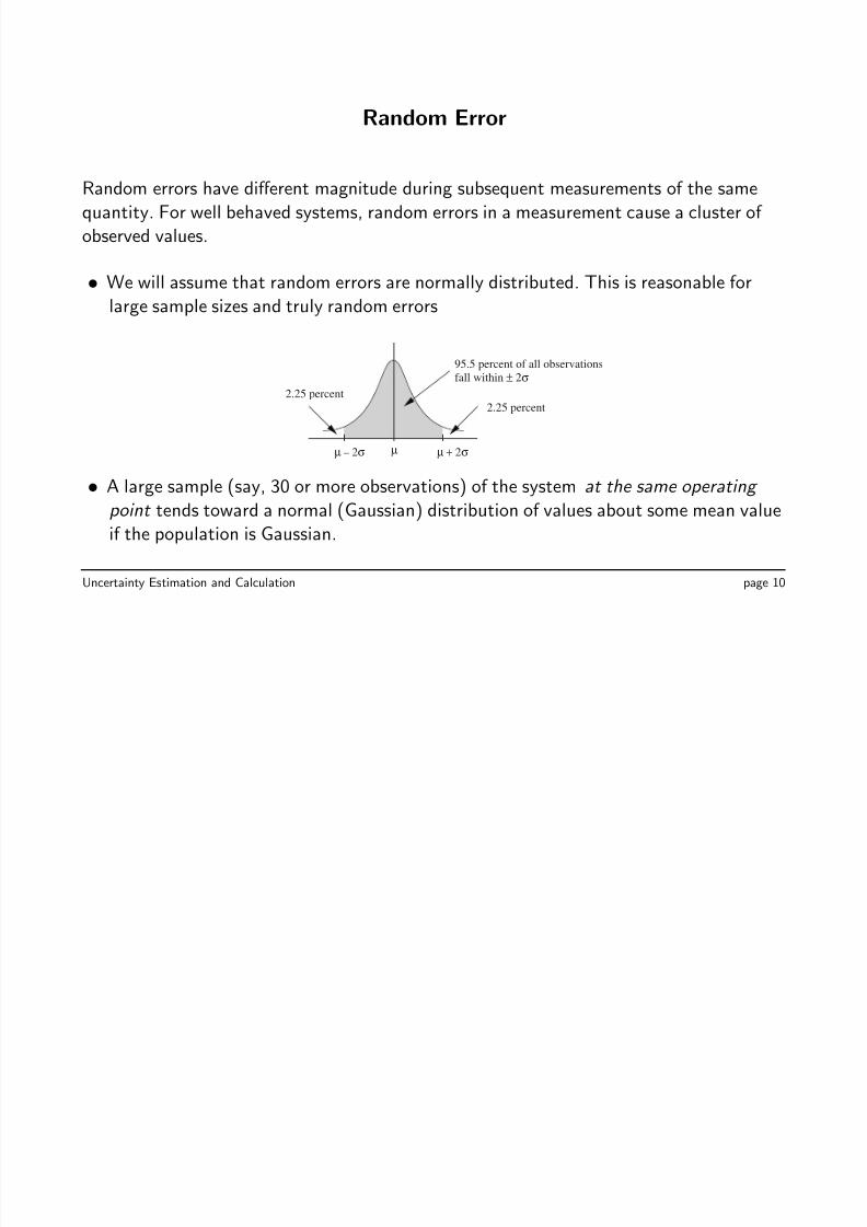
Random errors have different magnitude during subsequent measurements of the same
quantity. For well behaved systems, random errors in a measurement cause a cluster of
observed values.
• We will assume that random errors are normally distributed. This is reasonable for
large sample sizes and truly random errors
µ µ + 2σµ – 2σ
95.5 percent of all observations
fall within ± 2σ
2.25 percent
2.25 percent
• A large sample (say, 30 or more observations) of the system at the same operating
point tends toward a normal (Gaussian) distribution of values about some mean value
if the population is Gaussian.
Uncertainty Estimation and Calculation page 10

8/10/2019 Uncertainty Slides
http://slidepdf.com/reader/full/uncertainty-slides 12/61
Variable but Deterministic Error (1)
Some errors that appear to be random can be caused by faulty measurement techniques
(e.g. aliasing) or the errors may be variable but deterministic .
• Errors change even though the system is at the same nominal operating point
• Errors may not be recognized as deterministic: variations between tests, or test
conditions, may seem random.
• Cause of these errors are initially hidden from the experimenter
Uncertainty Estimation and Calculation page 11
8/10/2019 Uncertainty Slides
http://slidepdf.com/reader/full/uncertainty-slides 13/61
Variable but Deterministic Error (2)
Examples:
• Variations in room air conditions such as temperature and air circulation patterns
set-back thermostats
solar radiation through windows
presence of people in the room windows open to outside
• Changes in sensors
Thermal drift of sensors
Use of a new batch of thermocouple wire with different calibration
Cold working of thermocouple wire
• Changes in consumable materials or equipment used in experiments
Leakage or chemical degradation of working fluid
Mechanical wear or misalignment of positioning equipment
Uncertainty Estimation and Calculation page 12
8/10/2019 Uncertainty Slides
http://slidepdf.com/reader/full/uncertainty-slides 14/61
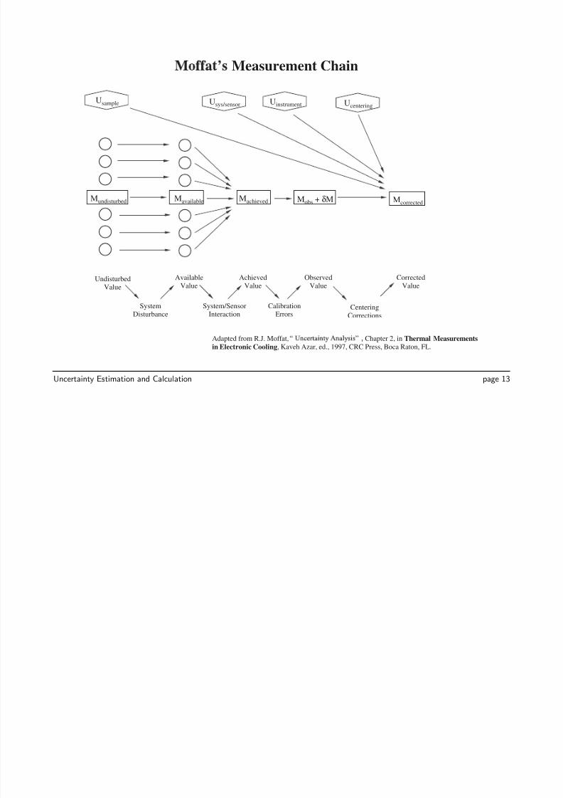
Mundisturbed Mavailable Machieved Mobs + δM Mcorrected
Adapted from R.J. Moffat, Chapter 2, in Thermal Measurements
in Electronic Cooling, Kaveh Azar, ed., 1997, CRC Press, Boca Raton, FL.
UndisturbedValue
AvailableValue
AchievedValue
ObservedValue
CorrectedValue
SystemDisturbance
System/SensorInteraction
CalibrationErrors
Centering
Corrections
Usys/sensor Uinstrument UcenteringUsample
Measurement Chain
Uncertainty Estimation and Calculation page 13

8/10/2019 Uncertainty Slides
http://slidepdf.com/reader/full/uncertainty-slides 15/61
Values of Measurand Along the Chain (1)
Mundisturbed ... Mcorrected
1. Undisturbed value: The value of quantity to be measured in a system with no
sensors.
Example : Temperature at point (x , y, z) is T (x , y, z).
2. Available value: The value of quantity to be measured after the sensor has been
placed in the system.
Example : Temperature at point (x , y, z) after sensor is been inserted is
T A(x , y, z) = T (x , y, z).
3. Achieved value: The value of quantity to be measured actually experienced by the
sensor.
Example : Temperature at the junction of a thermocouple at point (x , y, z) is
T j(x , y, z) = T A(x , y, z).
Uncertainty Estimation and Calculation page 14

8/10/2019 Uncertainty Slides
http://slidepdf.com/reader/full/uncertainty-slides 16/61
Values of Measurand Along the Chain (2)
4. Observed value: The value indicated by the instrumentation.
Example : EMF produced by thermocouple with temperature at T j(x , y, z) is
E j(x , y, z). The temperature indicated by the thermocouple is T i = f (E j), and
T i = T j(x , y, z) = T A(x , y, z) = T (x , y, z).
5. Corrected value: The value obtained after making centering corrections to the
observed value.
Example : T c = T i + ∆T where ∆T is a centering correction to account primarily
for the difference T j − T A. We design a model for the centering correction so that T cis closer to T than T i.
Uncertainty Estimation and Calculation page 15
8/10/2019 Uncertainty Slides
http://slidepdf.com/reader/full/uncertainty-slides 17/61
Contributions to Uncertainty of Measurand (1)
UcenteringUsample ...
1. Sampling Uncertainty
The undisturbed value is one of a large population of possible values for the
undisturbed quantity of interest.
Sampling Uncertainty is due to random errors.
2. System Sensor Uncertainty
• System disturbance changes the state of the system
• The sensor experiences interactions with the environment, e.g., radiation and
conduction effects on thermocouple measurement.System Sensor Uncertainty is due to a fixed error.
Uncertainty Estimation and Calculation page 16
8/10/2019 Uncertainty Slides
http://slidepdf.com/reader/full/uncertainty-slides 18/61
Contributions to Uncertainty of Measurand (2)
3. Instrument UncertaintiesEstimates of instrumentation uncertainties are readily made, though not all such
estimates reflect the true uncertainty. Moffat claims that with modern
instrumentation, the instrument uncertainties are often the least significant.
Instrument Uncertainties are due to random errors for a properly calibrated
instrument .
4. Centering Uncertainties
Each centering correction has an associated uncertainty. These must be included in a
final estimate of the uncertainty in the value of the measured quantity.
Centering Uncertainties are due to fixed errors. We accept these fixed errors after we
have done our best to minimize them.
Uncertainty Estimation and Calculation page 17
8/10/2019 Uncertainty Slides
http://slidepdf.com/reader/full/uncertainty-slides 19/61
Estimating Uncertainties (1)
1. System Disturbance Errors: The presence of a sensor changes the system
• Can be estimated, but not with any certainty
• Use estimates of disturbance errors to design the experiment, and to inform the
installation of sensors in the experimental apparatus. For example, locate a probe
to minimize flow blockage, or leakage.
• Goal is to design, build and instrument the system to minimize system disturbance
errors.
2. System/Sensor Interaction Errors: System phenomena alter value sensed by the
sensor.
Example: Radiation from the walls of a duct alter the temperature of an exposed
thermocouple junction used to measure the temperature of a flowing gas.• Should be estimated using engineering models of heat transfer and fluid flow
• Uncertainty in the estimate of this error needs to be included in final uncertainty
estimate for the quantity of interest.
Uncertainty Estimation and Calculation page 18
8/10/2019 Uncertainty Slides
http://slidepdf.com/reader/full/uncertainty-slides 20/61
Estimating Uncertainties (2)
3. Instrumentation Errors:
• Use manufacturer’s data or traceable calibration.
• Best solution is to perform simple benchmark experiments to measure the
instrument errors in situ .
• See Figure 4, page 61 in the article by Moffat [3] for a detailed worksheet used to
estimate the instrumentation error. Note that this worksheet does not included
system disturbance, system/sensor interactions, or conceptual errors.
4. Uncertainties in Centering Corrections:
• Report corrected values!
• Uncertainty in the correction should be smaller than the correction itself.
Uncertainty Estimation and Calculation page 19
8/10/2019 Uncertainty Slides
http://slidepdf.com/reader/full/uncertainty-slides 21/61
Estimating Uncertainties (3)
5. Conceptual Errors:
• Can be very large
• Not subjected to laws of physics
• Minimize by using good practice
Check units. Use shakedown experiments to compare results to established benchmarks.
Use redundant measurements, e.g. energy balances on both sides of an heat
exchanger.
Publish results with sufficient information so that others can replicate your
results.
6. Overall Errors
• Combine with methods presented below
• Use root-mean-squared procedure.
Uncertainty Estimation and Calculation page 20
8/10/2019 Uncertainty Slides
http://slidepdf.com/reader/full/uncertainty-slides 22/61
Example of Centering Correction (1)
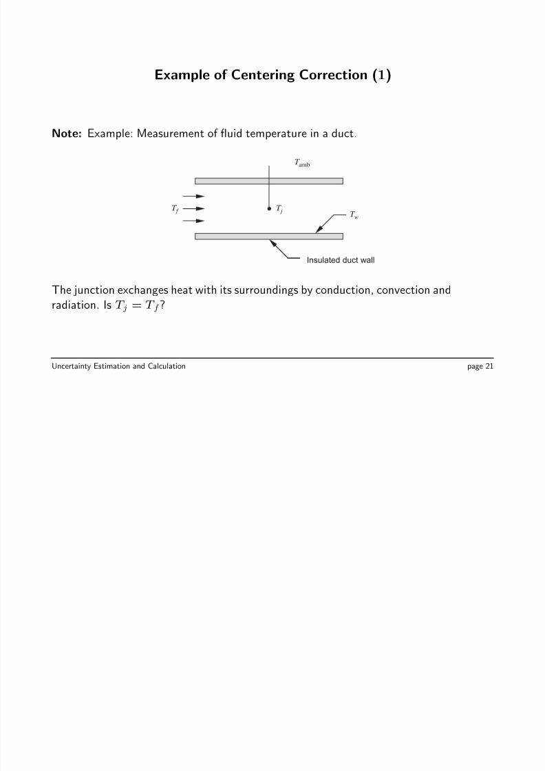
Note: Example: Measurement of fluid temperature in a duct.
T amb
T wT f T j
The junction exchanges heat with its surroundings by conduction, convection andradiation. Is T j = T f ?
Uncertainty Estimation and Calculation page 21
8/10/2019 Uncertainty Slides
http://slidepdf.com/reader/full/uncertainty-slides 23/61
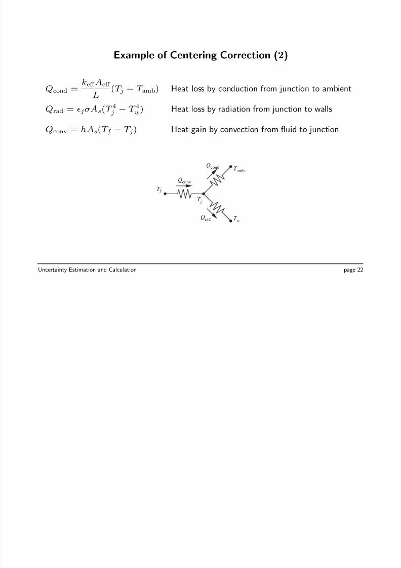
Example of Centering Correction (2)
Qcond = keff Aeff
L(T j − T amb) Heat loss by conduction from junction to ambient
Qrad = jσAs(T 4j − T 4w) Heat loss by radiation from junction to walls
Qconv = hAs(T f − T j) Heat gain by convection from fluid to junction
Qconv
Qcond
Qrad T w
T amb
T j
T f
Uncertainty Estimation and Calculation page 22
8/10/2019 Uncertainty Slides
http://slidepdf.com/reader/full/uncertainty-slides 24/61
Example of Centering Correction (3)
Steady state energy balance: Heat gain = heat loss
Qconv = Qcond + Qrad
For simplicity we will neglect radiation. This is a good assumption if T w ≈ T j.
Qconv = Qcond =⇒ keff Aeff
L(T j − T amb) = hAs(T f − T j)
Solve for T j
T j =
T f + keff Aeff
LhAs
T amb
1 + keff Aeff LhAs
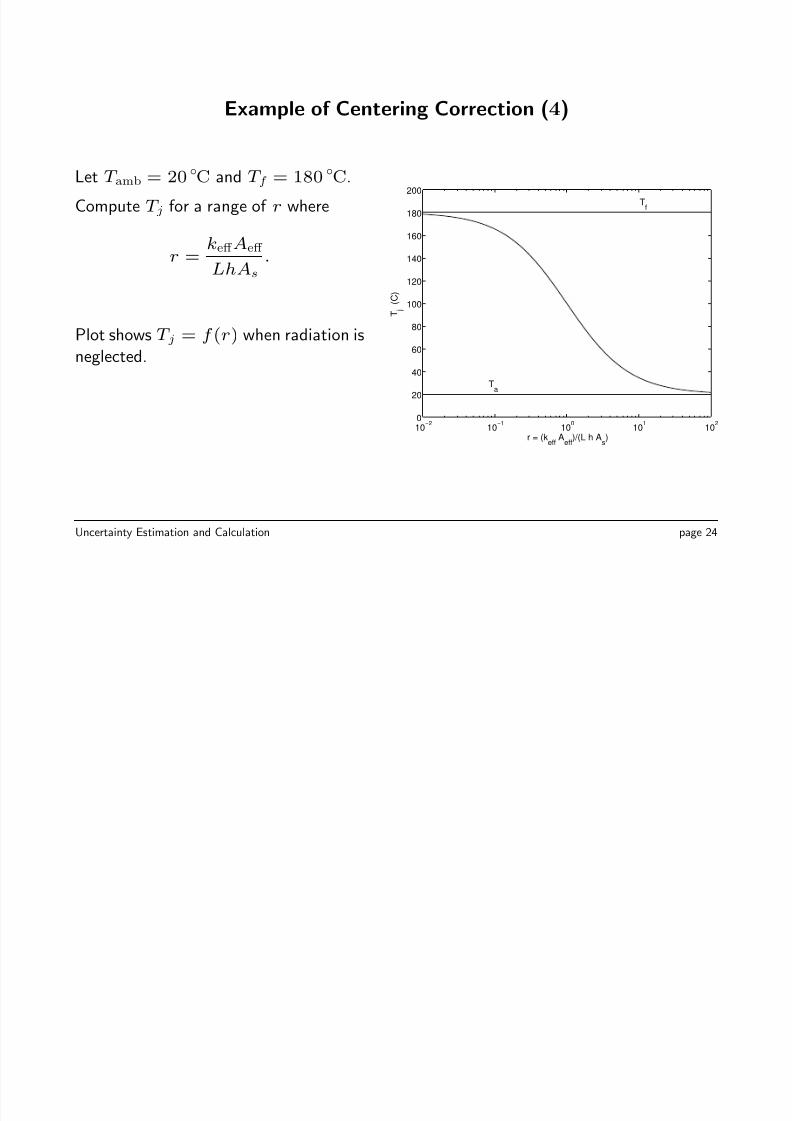
If conductivity or cross-section of the probe is large, then T j is closer to T amb than to T f .
Uncertainty Estimation and Calculation page 23
8/10/2019 Uncertainty Slides
http://slidepdf.com/reader/full/uncertainty-slides 25/61
Example of Centering Correction (4)
Let T amb = 20 C and T f = 180 C.
Compute T j for a range of r where
r = keff Aeff
LhAs
.
Plot shows T j = f (r) when radiation is
neglected.
10−2
10−1
100
101
1020
20
40
60
80
100
120
140
160
180
200
r = (keff
Aeff
)/(L h As)
T j
( C )
Ta
Tf
Uncertainty Estimation and Calculation page 24
8/10/2019 Uncertainty Slides
http://slidepdf.com/reader/full/uncertainty-slides 26/61
Example of Centering Correction (5)
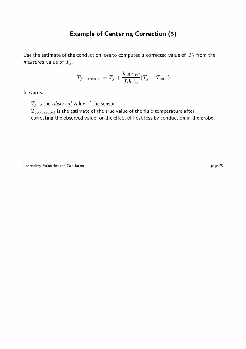
Use the estimate of the conduction loss to computed a corrected value of T f from the
measured value of T j.
T f,corrected = T j + keff Aeff
LhAs
(T j − T amb)
In words:
T j is the observed value of the sensor.
T f,corrected is the estimate of the true value of the fluid temperature after
correcting the observed value for the effect of heat loss by conduction in the probe.
Uncertainty Estimation and Calculation page 25

8/10/2019 Uncertainty Slides
http://slidepdf.com/reader/full/uncertainty-slides 27/61
Computing Uncertainty of Measurement
1. Definitions
2. Root-sum-squared Computation
3. Numerical approximation to sensitivities
4. Sequential perturbation method
Uncertainty Estimation and Calculation page 26
8/10/2019 Uncertainty Slides
http://slidepdf.com/reader/full/uncertainty-slides 28/61
Definitions
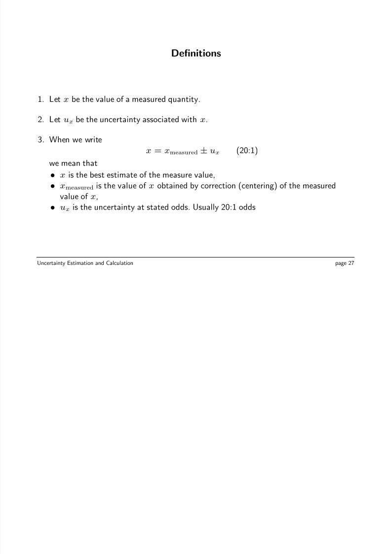
1. Let x be the value of a measured quantity.
2. Let ux be the uncertainty associated with x.
3. When we writex = xmeasured ± ux (20:1)
we mean that
• x is the best estimate of the measure value,
• xmeasured is the value of x obtained by correction (centering) of the measured
value of x,
• ux is the uncertainty at stated odds. Usually 20:1 odds
Uncertainty Estimation and Calculation page 27
8/10/2019 Uncertainty Slides
http://slidepdf.com/reader/full/uncertainty-slides 29/61
Meaning of 20:1 odds
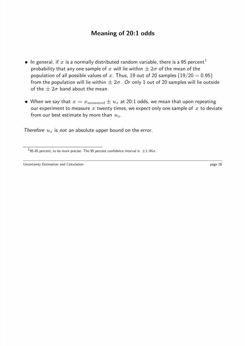
• In general, if x is a normally distributed random variable, there is a 95 percent1
probability that any one sample of x will lie within ± 2σ of the mean of the
population of all possible values of x. Thus, 19 out of 20 samples (19/20 = 0.95)
from the population will lie within
±2σ. Or only 1 out of 20 samples will lie outside
of the ± 2σ band about the mean.
• When we say that x = xmeasured ± ux at 20:1 odds, we mean that upon repeating
our experiment to measure x twenty times, we expect only one sample of x to deviate
from our best estimate by more than ux.
Therefore ux is not an absolute upper bound on the error.
195.45 percent, to be more precise. The 95 percent confidence interval is ±1.96σ.
Uncertainty Estimation and Calculation page 28
8/10/2019 Uncertainty Slides
http://slidepdf.com/reader/full/uncertainty-slides 30/61
8/10/2019 Uncertainty Slides
http://slidepdf.com/reader/full/uncertainty-slides 31/61
Computational Procedures (1)
The analytical method involves deriving a single formula for the uncertainty in a
measurement.
• Straightforward computation
• Becomes unwieldy and eventually impractical as the data reduction procedure
becomes increasingly complex.
The sequential perturbation technique is easy to implement when the data reduction
procedure is automated via a computer program.
• Uncertainty estimate is approximate, not exact as in the analytical method.
• Is simple to implement, and allows for evolution of the model underlying the datareduction.
Uncertainty Estimation and Calculation page 30
8/10/2019 Uncertainty Slides
http://slidepdf.com/reader/full/uncertainty-slides 32/61
Root-Sum-Squared (RSS) Computation (1)
Begin with the basic definition of the Root-Sum-Squared uncertainty.
The data reduction computation is represented by
R = f (x1, x2, . . . , xn)
where R is the final, measured result , and xi are measured quantities. Let ui be the
uncertainty in xi so that
xi = xmeasured,i ± ui
This is a slight change in notation to avoid the double subscript uxi
Uncertainty Estimation and Calculation page 31
8/10/2019 Uncertainty Slides
http://slidepdf.com/reader/full/uncertainty-slides 33/61
Root-Sum-Squared (RSS) Computation (2)
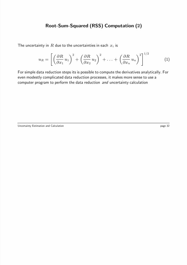
The uncertainty in R due to the uncertainties in each xi is
uR =
∂R
∂x1
u12
+ ∂R
∂x2
u22
+ . . . + ∂R
∂xn
un21/2
(1)
For simple data reduction steps its is possible to compute the derivatives analytically. For
even modestly complicated data reduction processes, it makes more sense to use a
computer program to perform the data reduction and uncertainty calculation
Uncertainty Estimation and Calculation page 32
8/10/2019 Uncertainty Slides
http://slidepdf.com/reader/full/uncertainty-slides 34/61
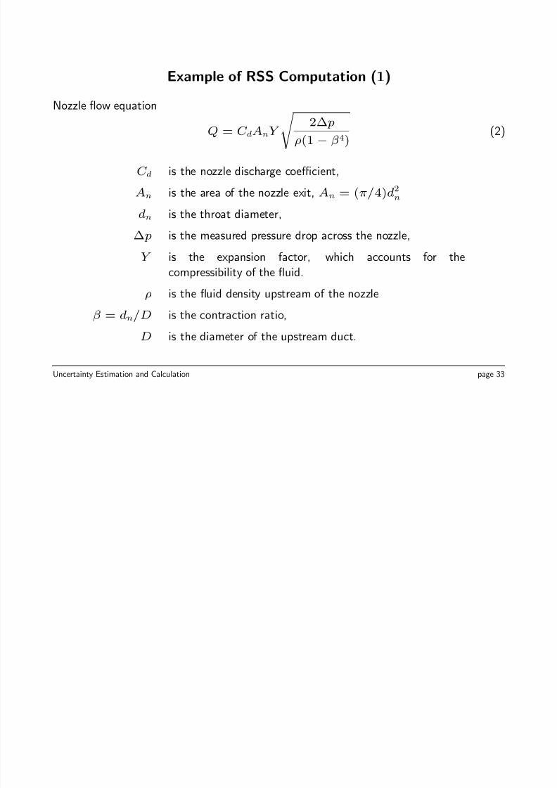
Example of RSS Computation (1)
Nozzle flow equation
Q = C dAnY
2∆ p
ρ(1 − β4) (2)
C d is the nozzle discharge coefficient,
An is the area of the nozzle exit, An = (π/4)d
2
n
dn is the throat diameter,
∆ p is the measured pressure drop across the nozzle,
Y is the expansion factor, which accounts for the
compressibility of the fluid.
ρ is the fluid density upstream of the nozzleβ = dn/D is the contraction ratio,
D is the diameter of the upstream duct.
Uncertainty Estimation and Calculation page 33
8/10/2019 Uncertainty Slides
http://slidepdf.com/reader/full/uncertainty-slides 35/61
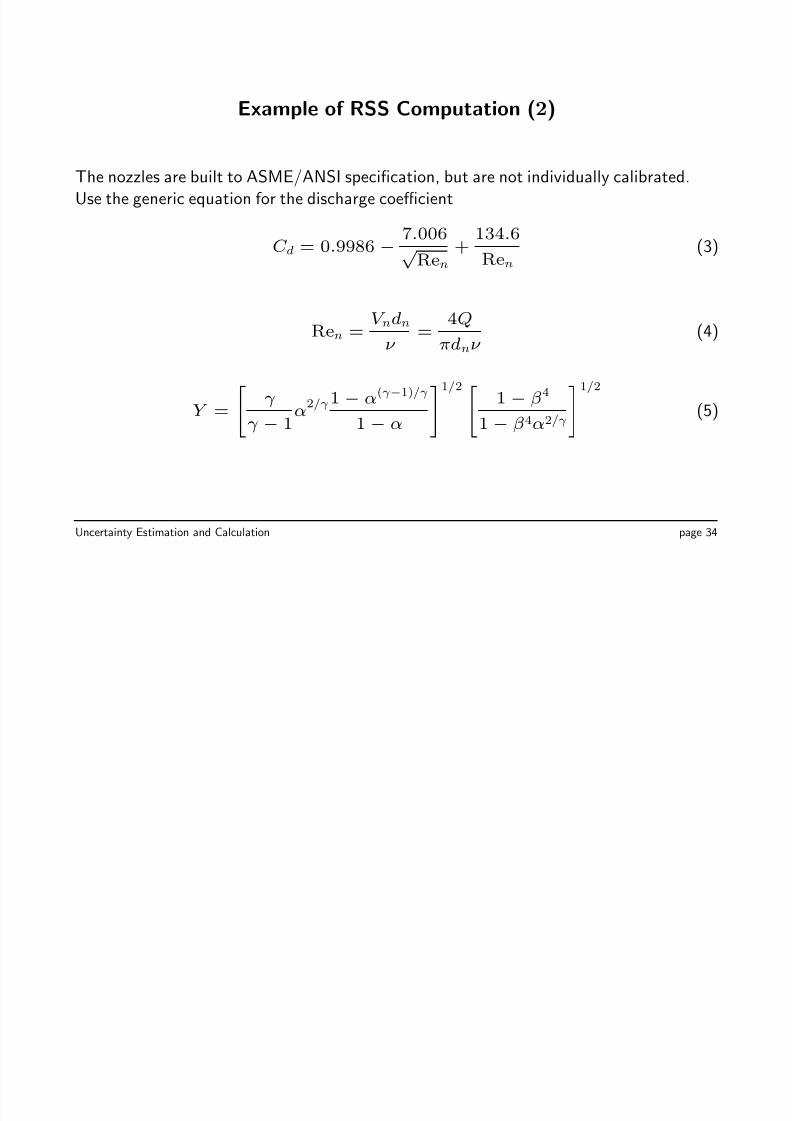
Example of RSS Computation (2)
The nozzles are built to ASME/ANSI specification, but are not individually calibrated.
Use the generic equation for the discharge coefficient
C d = 0.9986 − 7.006√ Ren
+ 134.6
Ren
(3)
Ren = V ndn
ν =
4Q
πdnν (4)
Y = γ
γ − 1α
2/γ 1
−α(γ −1)/γ
1 − α
1/2
1
−β4
1 − β4α2/γ
1/2
(5)
Uncertainty Estimation and Calculation page 34
8/10/2019 Uncertainty Slides
http://slidepdf.com/reader/full/uncertainty-slides 36/61
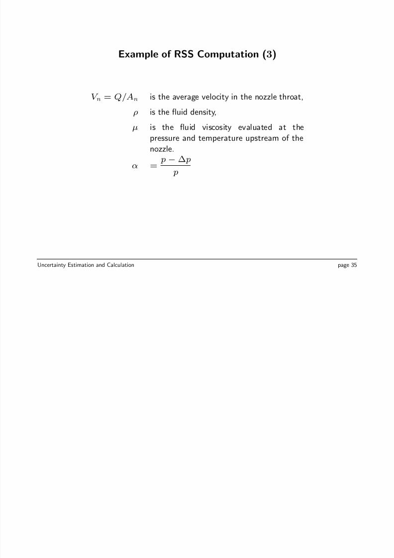
Example of RSS Computation (3)
V n = Q/An is the average velocity in the nozzle throat,
ρ is the fluid density,
µ is the fluid viscosity evaluated at the
pressure and temperature upstream of thenozzle.
α = p − ∆ p
p
Uncertainty Estimation and Calculation page 35
8/10/2019 Uncertainty Slides
http://slidepdf.com/reader/full/uncertainty-slides 37/61
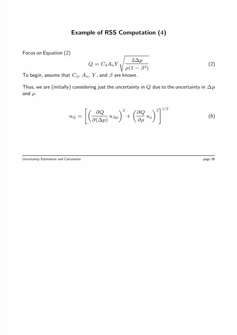
Example of RSS Computation (4)
Focus on Equation (2)
Q = C dAnY
2∆ p
ρ(1 − β4) (2)
To begin, assume that C d, An, Y , and β are known.
Thus, we are (initially) considering just the uncertainty in Q due to the uncertainty in ∆ p
and ρ.
uQ =
∂Q
∂ (∆ p) u∆ p
2
+
∂Q
∂ρuρ
21/2
(6)
Uncertainty Estimation and Calculation page 36
8/10/2019 Uncertainty Slides
http://slidepdf.com/reader/full/uncertainty-slides 38/61
Example of RSS Computation (5)
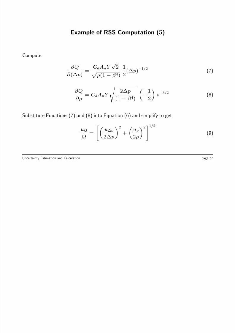
Compute:
∂Q
∂ (∆ p) =
C dAnY √
2
ρ(1 − β4)
1
2(∆ p)−1/2 (7)
∂Q
∂ρ= C dAnY
2∆ p
(1 − β4)
−1
2
ρ−3/2 (8)
Substitute Equations (7) and (8) into Equation (6) and simplify to get
uQ
Q=
u∆ p
2∆ p
2
+
uρ
2ρ
21/2
(9)
Uncertainty Estimation and Calculation page 37
8/10/2019 Uncertainty Slides
http://slidepdf.com/reader/full/uncertainty-slides 39/61
Example of RSS Computation (6)
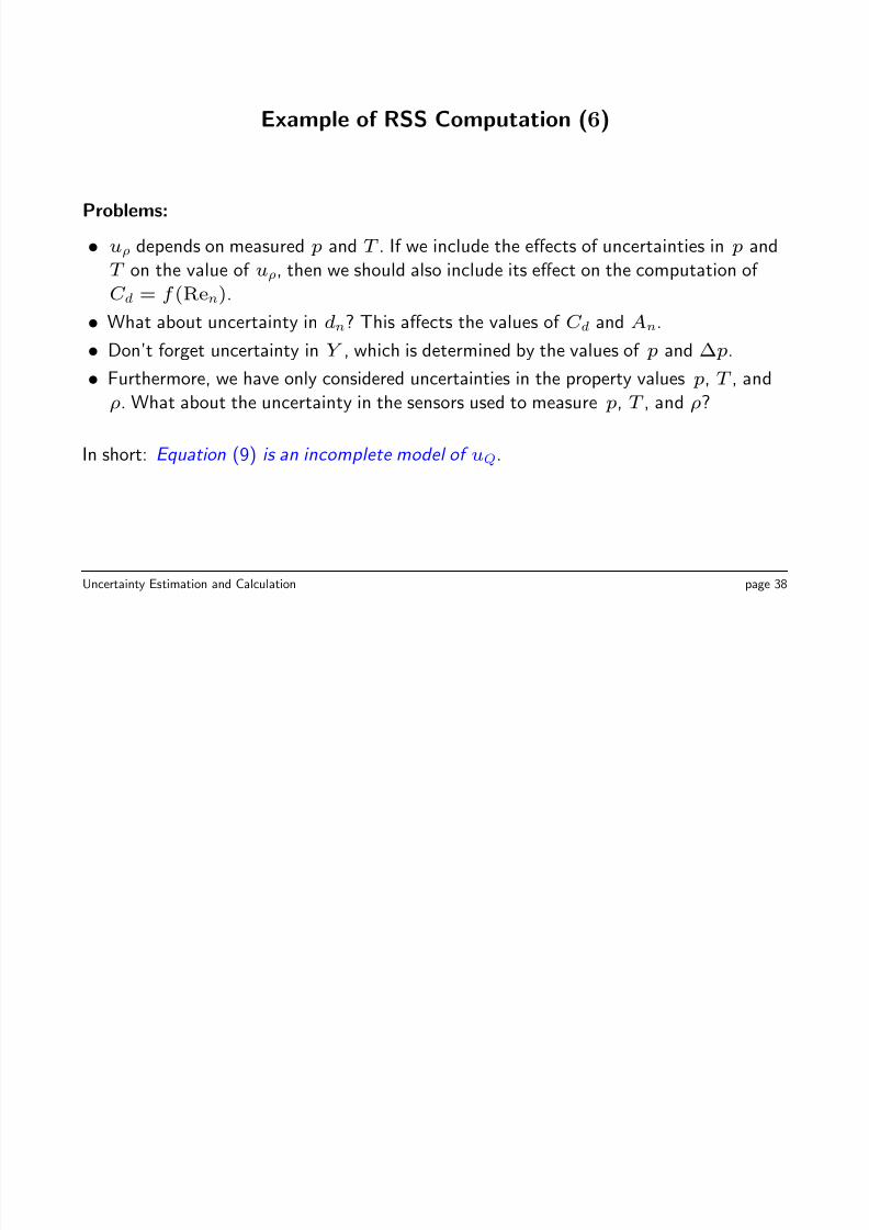
Problems:
• uρ depends on measured p and T . If we include the effects of uncertainties in p and
T on the value of uρ, then we should also include its effect on the computation of
C d = f (Ren).
• What about uncertainty in dn? This affects the values of C d and An.
• Don’t forget uncertainty in Y , which is determined by the values of p and ∆ p.
• Furthermore, we have only considered uncertainties in the property values p, T , and
ρ. What about the uncertainty in the sensors used to measure p, T , and ρ?
In short: Equation (9) is an incomplete model of uQ.
Uncertainty Estimation and Calculation page 38
8/10/2019 Uncertainty Slides
http://slidepdf.com/reader/full/uncertainty-slides 40/61
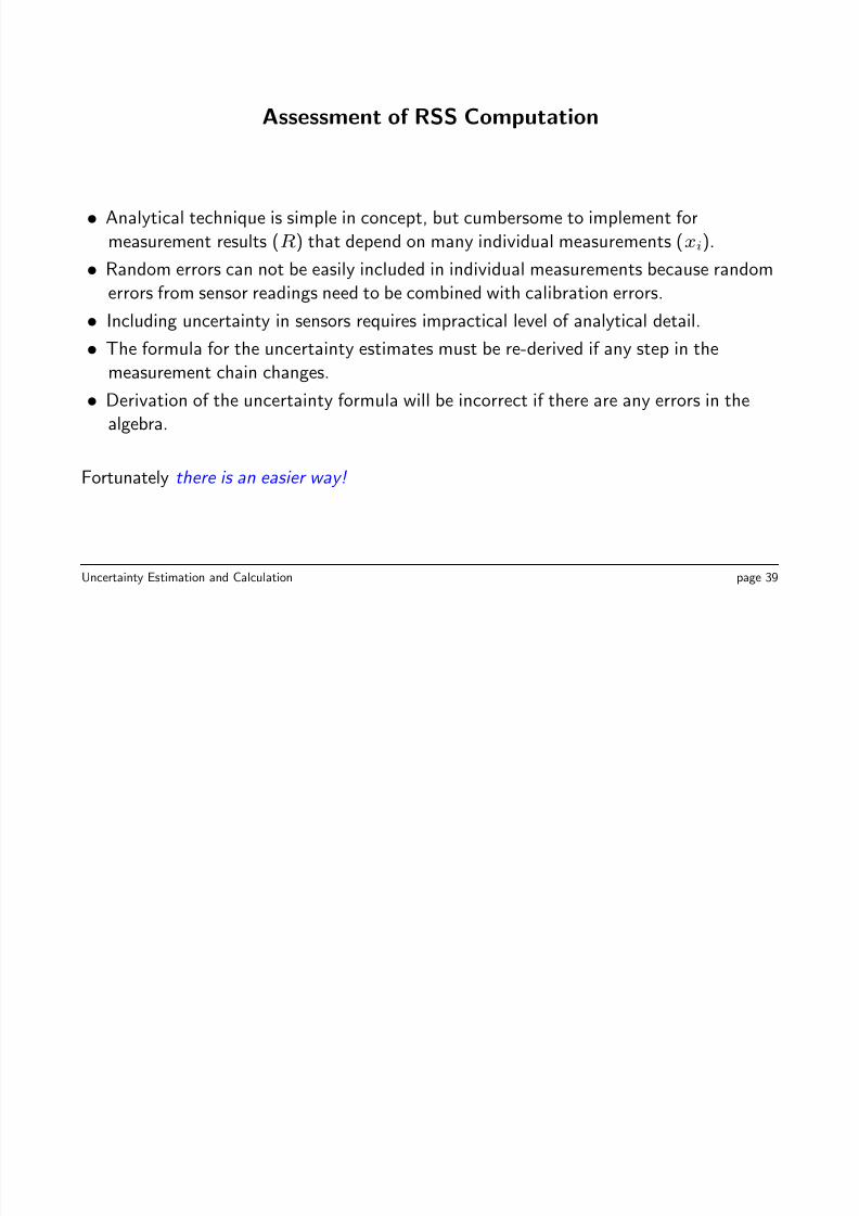
Assessment of RSS Computation
• Analytical technique is simple in concept, but cumbersome to implement for
measurement results (R) that depend on many individual measurements (xi).
• Random errors can not be easily included in individual measurements because random
errors from sensor readings need to be combined with calibration errors.
• Including uncertainty in sensors requires impractical level of analytical detail.
• The formula for the uncertainty estimates must be re-derived if any step in the
measurement chain changes.
• Derivation of the uncertainty formula will be incorrect if there are any errors in the
algebra.
Fortunately there is an easier way!
Uncertainty Estimation and Calculation page 39
8/10/2019 Uncertainty Slides
http://slidepdf.com/reader/full/uncertainty-slides 41/61
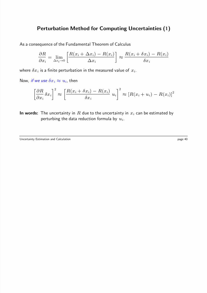
Perturbation Method for Computing Uncertainties (1)
As a consequence of the Fundamental Theorem of Calculus
∂R
∂xi
= lim∆xi→0
R(xi + ∆xi) − R(xi)
∆xi
≈ R(xi + δxi) − R(xi)
δxi
where δxi is a finite perturbation in the measured value of xi.
Now, if we use δxi ≈ ui, then
∂R
∂xi
δxi
2
≈
R(xi + δxi) − R(xi)
δxi
ui
2
≈ [R(xi + ui) − R(xi)]2
In words: The uncertainty in R due to the uncertainty in xi can be estimated by
perturbing the data reduction formula by ui.
Uncertainty Estimation and Calculation page 40
8/10/2019 Uncertainty Slides
http://slidepdf.com/reader/full/uncertainty-slides 42/61
Perturbation Method for Computing Uncertainties (2)
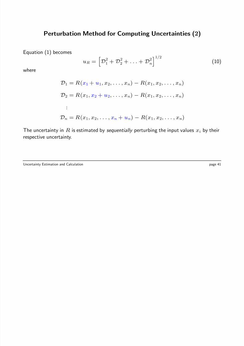
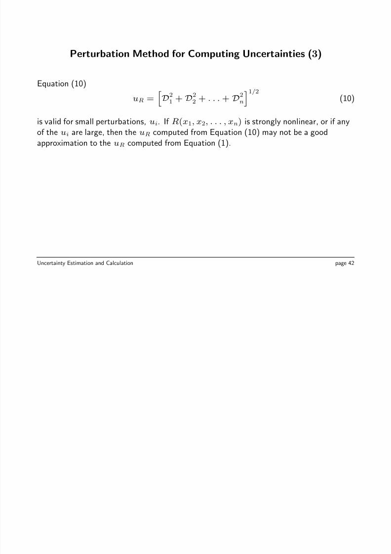
Equation (1) becomes
uR =D2
1 + D22 + . . . + D2
n
1/2
(10)
where
D1 = R(x1 + u1, x2, . . . , xn)
−R(x1, x2, . . . , xn)
D2 = R(x1, x2 + u2, . . . , xn) − R(x1, x2, . . . , xn)
...
Dn = R(x1, x2, . . . , xn + un) − R(x1, x2, . . . , xn)
The uncertainty in R is estimated by sequentially perturbing the input values xi by theirrespective uncertainty.
Uncertainty Estimation and Calculation page 41
8/10/2019 Uncertainty Slides
http://slidepdf.com/reader/full/uncertainty-slides 43/61
8/10/2019 Uncertainty Slides
http://slidepdf.com/reader/full/uncertainty-slides 44/61
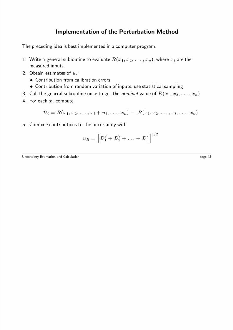
Implementation of the Perturbation Method
The preceding idea is best implemented in a computer program.
1. Write a general subroutine to evaluate R(x1, x2, . . . , xn), where xi are the
measured inputs.
2. Obtain estimates of ui:
• Contribution from calibration errors
• Contribution from random variation of inputs: use statistical sampling
3. Call the general subroutine once to get the nominal value of R(x1, x2, . . . , xn)
4. For each xi compute
Di = R(x1, x2, . . . , xi + ui, . . . , xn) − R(x1, x2, . . . , xi, . . . , xn)
5. Combine contributions to the uncertainty with
uR =D2
1 + D22 + . . . + D2
n
1/2
Uncertainty Estimation and Calculation page 43
8/10/2019 Uncertainty Slides
http://slidepdf.com/reader/full/uncertainty-slides 45/61
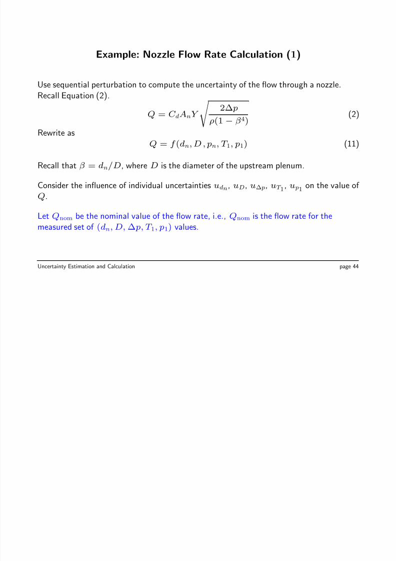
Example: Nozzle Flow Rate Calculation (1)
Use sequential perturbation to compute the uncertainty of the flow through a nozzle.
Recall Equation (2).
Q = C dAnY
2∆ p
ρ(1 − β4) (2)
Rewrite as
Q = f (dn, D , pn, T 1, p1) (11)
Recall that β = dn/D, where D is the diameter of the upstream plenum.
Consider the influence of individual uncertainties udn, uD, u∆ p, uT 1, u p1
on the value of
Q.
Let Qnom be the nominal value of the flow rate, i.e., Qnom is the flow rate for the
measured set of (dn, D, ∆ p, T 1, p1) values.
Uncertainty Estimation and Calculation page 44
8/10/2019 Uncertainty Slides
http://slidepdf.com/reader/full/uncertainty-slides 46/61
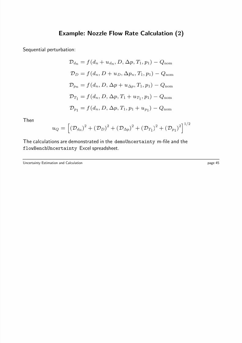
Example: Nozzle Flow Rate Calculation (2)
Sequential perturbation:
Ddn = f (dn + udn, D, ∆ p, T 1, p1) − Qnom
DD = f (dn, D + uD, ∆ pn, T 1, p1) − Qnom
D pn = f (dn, D, ∆ p + u∆ p, T 1, p1) − Qnom
DT 1 = f (dn, D, ∆ p, T 1 + uT 1
, p1) − Qnom
D p1 = f (dn, D, ∆ p, T 1, p1 + u p1
) − Qnom
Then
uQ =
(Ddn)2
+ (DD)2
+ (D∆ p)2
+ (DT 1)2
+ (D p1)21/2
The calculations are demonstrated in the demoUncertainty m-file and the
flowBenchUncertainty Excel spreadsheet.
Uncertainty Estimation and Calculation page 45
8/10/2019 Uncertainty Slides
http://slidepdf.com/reader/full/uncertainty-slides 47/61
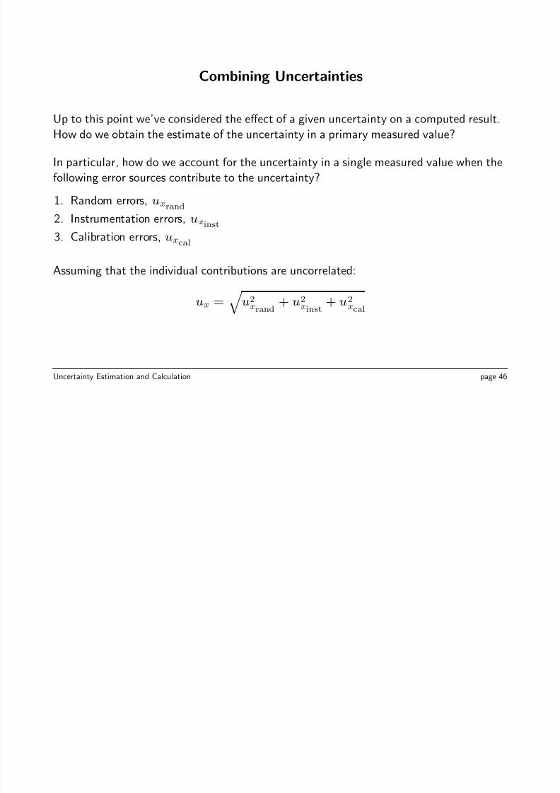
Combining Uncertainties
Up to this point we’ve considered the effect of a given uncertainty on a computed result.
How do we obtain the estimate of the uncertainty in a primary measured value?
In particular, how do we account for the uncertainty in a single measured value when the
following error sources contribute to the uncertainty?
1. Random errors, uxrand
2. Instrumentation errors, uxinst
3. Calibration errors, uxcal
Assuming that the individual contributions are uncorrelated:
ux =
u2xrand + u2xinst + u2xcal
Uncertainty Estimation and Calculation page 46
8/10/2019 Uncertainty Slides
http://slidepdf.com/reader/full/uncertainty-slides 48/61
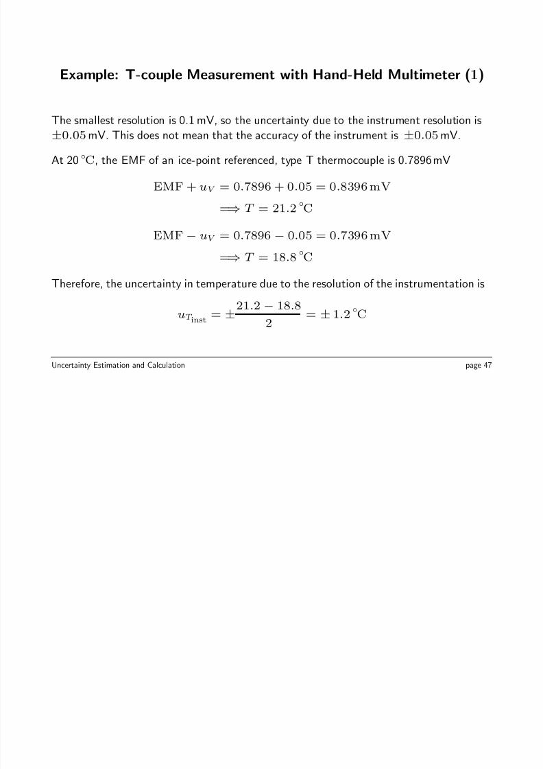
Example: T-couple Measurement with Hand-Held Multimeter (1)
The smallest resolution is 0.1 mV, so the uncertainty due to the instrument resolution is
±0.05 mV. This does not mean that the accuracy of the instrument is ±0.05 mV.
At 20 C, the EMF of an ice-point referenced, type T thermocouple is 0.7896 mV
EMF + uV = 0.7896 + 0.05 = 0.8396 mV
=⇒ T = 21.2C
EMF− uV = 0.7896 − 0.05 = 0.7396 mV
=⇒ T = 18.8 C
Therefore, the uncertainty in temperature due to the resolution of the instrumentation is
uT inst = ±21.2 − 18.8
2 = ± 1.2 C
Uncertainty Estimation and Calculation page 47
8/10/2019 Uncertainty Slides
http://slidepdf.com/reader/full/uncertainty-slides 49/61
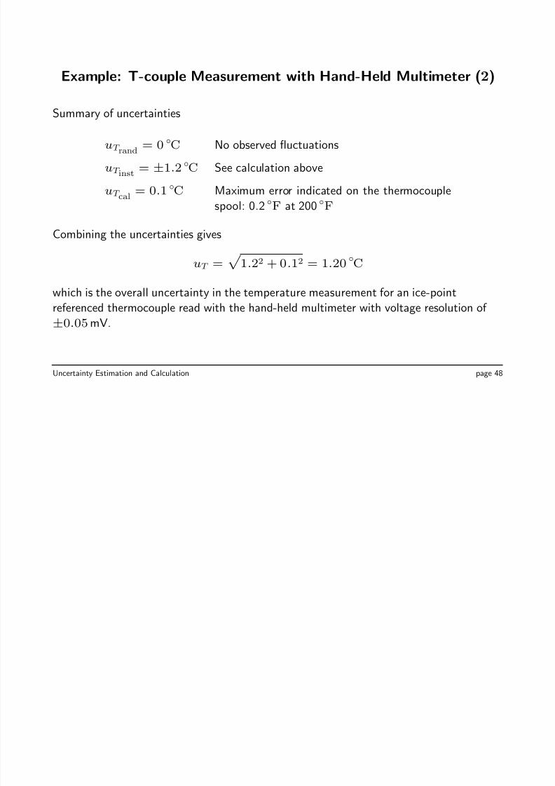
Example: T-couple Measurement with Hand-Held Multimeter (2)
Summary of uncertainties
uT rand = 0 C No observed fluctuations
uT inst = ±1.2 C See calculation above
uT cal
= 0.1 C Maximum error indicated on the thermocouple
spool: 0.2 F at 200 F
Combining the uncertainties gives
uT =
1.22 + 0.12 = 1.20 C
which is the overall uncertainty in the temperature measurement for an ice-pointreferenced thermocouple read with the hand-held multimeter with voltage resolution of
±0.05 mV.
Uncertainty Estimation and Calculation page 48
8/10/2019 Uncertainty Slides
http://slidepdf.com/reader/full/uncertainty-slides 50/61
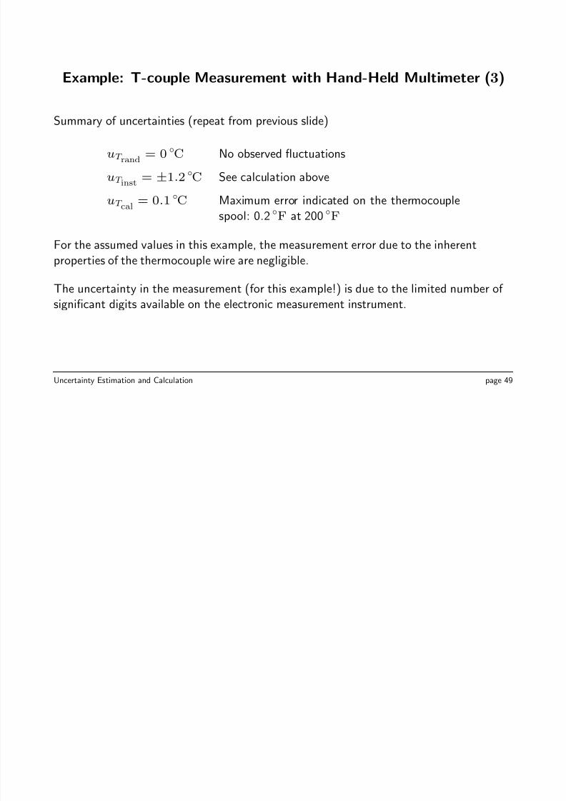
Example: T-couple Measurement with Hand-Held Multimeter (3)
Summary of uncertainties (repeat from previous slide)
uT rand = 0 C No observed fluctuations
uT inst = ±1.2 C See calculation above
uT cal = 0.1 C Maximum error indicated on the thermocouplespool: 0.2 F at 200 F
For the assumed values in this example, the measurement error due to the inherent
properties of the thermocouple wire are negligible.
The uncertainty in the measurement (for this example!) is due to the limited number of
significant digits available on the electronic measurement instrument.
Uncertainty Estimation and Calculation page 49
8/10/2019 Uncertainty Slides
http://slidepdf.com/reader/full/uncertainty-slides 51/61
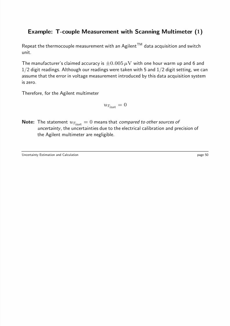
Example: T-couple Measurement with Scanning Multimeter (1)
Repeat the thermocouple measurement with an AgilentTM data acquisition and switch
unit.
The manufacturer’s claimed accuracy is ±0.005 µV with one hour warm up and 6 and
1/2 digit readings. Although our readings were taken with 5 and 1/2 digit setting, we can
assume that the error in voltage measurement introduced by this data acquisition system
is zero.
Therefore, for the Agilent multimeter
uT inst = 0
Note: The statement uT inst = 0 means that compared to other sources of uncertainty , the uncertainties due to the electrical calibration and precision of
the Agilent multimeter are negligible.
Uncertainty Estimation and Calculation page 50
8/10/2019 Uncertainty Slides
http://slidepdf.com/reader/full/uncertainty-slides 52/61
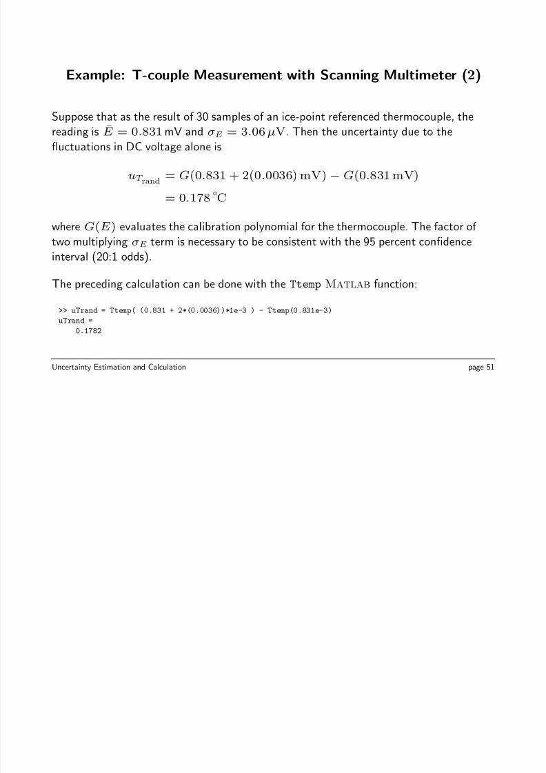
Example: T-couple Measurement with Scanning Multimeter (2)
Suppose that as the result of 30 samples of an ice-point referenced thermocouple, the
reading is E = 0.831 mV and σE = 3.06 µV. Then the uncertainty due to the
fluctuations in DC voltage alone is
uT rand = G(0.831 + 2(0.0036) mV)− G(0.831 mV)
= 0.178 C
where G(E ) evaluates the calibration polynomial for the thermocouple. The factor of
two multiplying σE term is necessary to be consistent with the 95 percent confidence
interval (20:1 odds).
The preceding calculation can be done with the Ttemp Matlab function:
>> uTrand = Ttemp( (0.831 + 2*(0.0036))*1e-3 ) - Ttemp(0.831e-3)
uTrand =
0.1782
Uncertainty Estimation and Calculation page 51

8/10/2019 Uncertainty Slides
http://slidepdf.com/reader/full/uncertainty-slides 53/61
Example: T-couple Measurement with Scanning Multimeter (3)
The calibration error for the thermocouple wire is ±0.1 C.
Finally, we combine the uncertainties due to random fluctuations in the signal, and the
uncertainty due to the wire calibration.
uT = u2T rand
+ u2T cal
(uT inst = 0)
=
0.1782 + 0.12 = 0.20 C
This is the overall uncertainty in the temperature measurement for an ice-point referenced
thermocouple read with the Agilent multimeter.
The uncertainty in the temperature measurement with the Agilent multimeter is an order
of magnitude less than the uncertainty in the temperature measurement with thehand-held multimeter. This result is primarily due to the much higher resolution of the
Agilent multimeter. Note that the calculations of uncertainty assumed that there was no
calibration errors in these instruments.
Uncertainty Estimation and Calculation page 52
8/10/2019 Uncertainty Slides
http://slidepdf.com/reader/full/uncertainty-slides 54/61
Example: T-couple Measurement with Scanning Multimeter (4)
What if the thermocouple is referenced to the zone box temperature and the temperature
of the zone box is measured with a thermistor?
Now, two streams of uncertainties contribute
• Calibration, instrument, and random uncertainty in the thermistor measurement.• Calibration, instrument, and random uncertainty in the thermocouple measurement.
Uncertainty Estimation and Calculation page 53

8/10/2019 Uncertainty Slides
http://slidepdf.com/reader/full/uncertainty-slides 55/61
Example: T-couple Measurement with Scanning Multimeter (5)
Suppose we have the following data taken when the system is assumed to be at steady
state
E = −1.15× 10⁻⁵ V average of 30 readings of the thermocouple
referenced to the zone box
σE = 2.97× 10⁻⁶ V standard deviation of 30 thermocouple readings
R = 10815.3 Ω average of 30 readings of the thermistor in the
zone box
σR = 4.0 Ω standard deviation of 30 thermistor readings
Uncertainty Estimation and Calculation page 54
8/10/2019 Uncertainty Slides
http://slidepdf.com/reader/full/uncertainty-slides 56/61

8/10/2019 Uncertainty Slides
http://slidepdf.com/reader/full/uncertainty-slides 57/61
Example: T-couple Measurement with Scanning Multimeter (7)
The calibration equation for the temperature reading is of the form
T = f (E, R)
where E is the EMF of the thermocouple, and R is the resistance of the thermistor.
Using the sequential perturbation technique, and assuming uT inst = 0 for both the
voltage and resistance measurements, the uncertainty in the temperature reading is
uT =
u2T rand,E
+ u2T rand,R
+ u2T cal
where
uT rand,E = f (E + 2σE , R) − f (E, R)
uT rand,R = f (E, R + 2σR) − f (E, R)
The factor of 2 in the perturbation gives an uncertainty estimate with 95 percent
confidence intervals (20:1 odds).
Uncertainty Estimation and Calculation page 56
8/10/2019 Uncertainty Slides
http://slidepdf.com/reader/full/uncertainty-slides 58/61
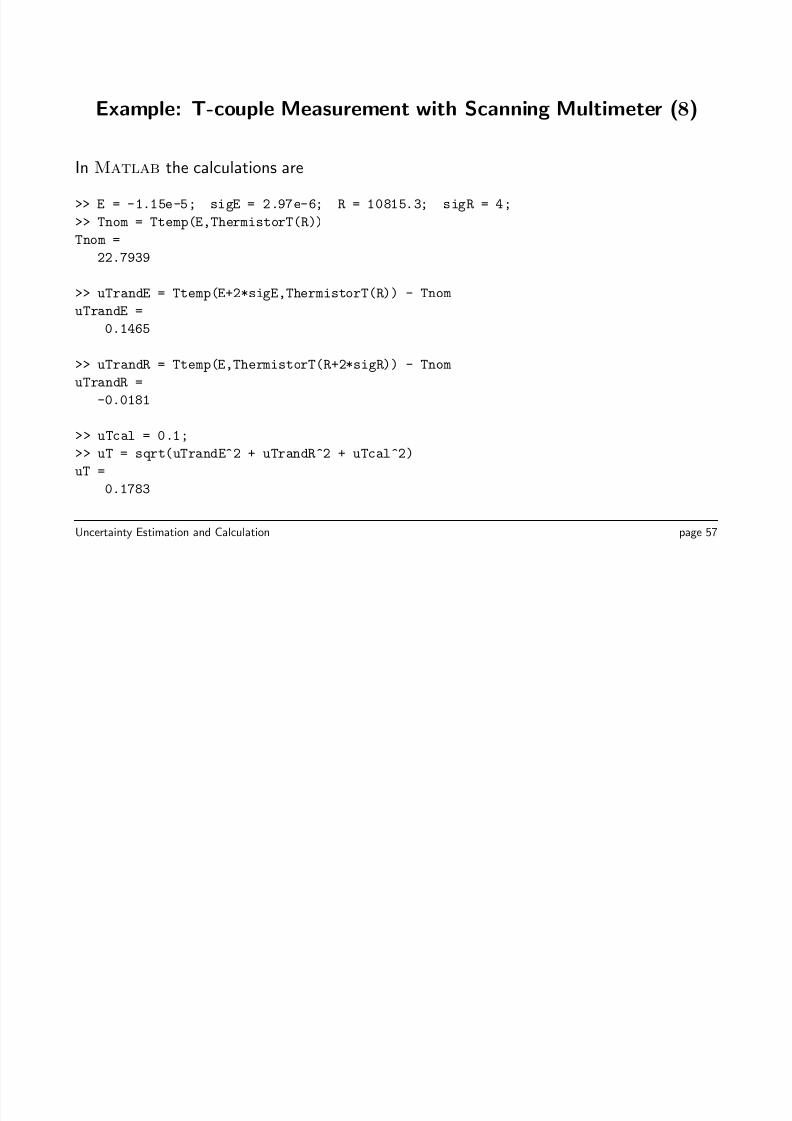
Example: T-couple Measurement with Scanning Multimeter (8)
In Matlab the calculations are
>> E = -1.15e-5; sigE = 2.97e-6; R = 10815.3; sigR = 4;
>> Tnom = Ttemp(E,ThermistorT(R))
Tnom =
22.7939
>> uTrandE = Ttemp(E+2*sigE,ThermistorT(R)) - Tnom
uTrandE =
0.1465
>> uTrandR = Ttemp(E,ThermistorT(R+2*sigR)) - Tnom
uTrandR =
-0.0181
>> uTcal = 0.1;
>> uT = sqrt(uTrandE^2 + uTrandR^2 + uTcal^2)
uT =
0.1783
Uncertainty Estimation and Calculation page 57
8/10/2019 Uncertainty Slides
http://slidepdf.com/reader/full/uncertainty-slides 59/61
Example: T-couple Measurement with Scanning Multimeter (9)
In Matlab the calculations give uT = 0.178 C.
From this calculation we conclude that the uncertainty in the temperature measurement is
±0.2 C at 20:1 odds.
Note that in the preceding calculations we have neglected errors in the curve fits to the
calibration data.
Uncertainty Estimation and Calculation page 58
8/10/2019 Uncertainty Slides
http://slidepdf.com/reader/full/uncertainty-slides 60/61
8/10/2019 Uncertainty Slides
http://slidepdf.com/reader/full/uncertainty-slides 61/61
References
[1] H. W. Coleman and J. Steele, W. Glenn. Experimentation and Uncertainty Analysis
for Engineers . Wiley, New York, 1999.
[2] R. J. Moffat. Using uncertainty analysis in the planning of an experiment. Journal of Fluids Engineering , 107:173–178, June 1985.
[3] R. J. Moffat. Uncertainty analysis. In K. Azar, editor, Thermal Measurements in
Electronic Cooling , pages 45–80. CRC Press, Boca Raton, FL, 1997.
[4] B. N. Taylor and C. E. Kuyatt. Guidelines for evaluating and expressing the
uncertainty of nist measurement results. NIST Technical Note TN 1297, National
Institute for Standards and Technology, Washington, DC, 1994.[5] J. R. Taylor. An Introduction to Error Analysis: The Study of Uncertainties in
Physical Measurements . University Science Books, Sausalito, CA, 1997.
Uncertainty Estimation and Calculation page 60