UNCLASS IFI1ED

CSRTECLSIFITION OF THIS PAGE A REPORT DOCUMENTATION PAGE

I& REPORT SECURITY CLASSIFICATION L RESTRICTIVE MARKINGS

Unclassified1 CUITV CLASSIFICATION AUTHORITY 3. DISTRIBUTION/AVAILABILITY OF REPORt

Approved for public release;L DEC.ASSIFICATIONIDOWNGRADING SCHEOULE distribution is unlimited

4. PERFORMING ORGANIZATION REPORT NUMBER(S) S. MONITORING ORGANIZATION REPORT NUMBER(S)

G& NAME OF PERFORMING ORGANIZATION b. OFFICE SYMBOL 7. NAME OF MONITORING ORGANIZATION(If .pplicabia)

Rondout Associates, Inc. AFTAC/TGRG. ADDRESS (C t,. State and ZIP Coda) 7b. ADDRESS (City. Stat. and ZIP Code)

P.O. Box 224 Patrick Air Force BaseStone Ridge, NY 12484 Florida 32925-6001

@&.NAME OF FUNOINGJSPONSORING Sb. OFFICE SYMBOL 9. PROCUREMENT INSTRUMENT IDENTIFICATION NUMBERORGANIZATION (if applicable)

DARPA GSDIII ADDRESS (01y. State and ZIP Code) 10. SOURCE OF FUNDING NOS.

1400 Wilson Boulevard PROGRAM PROJECT TASK WORK UNIT

Arlington, Virginia 22209 ELEMENTNO. NO. NO. No.

11. TITLE (Include Secur ty Clas-tio,-nj 62714 E DT/5126 All 6A10Source Depths Utilizing Broad Band Data

12. PERSONAL AUTHOR(S)

George H. Sutton, PI, Jerry A. Carter, Noel Barstow13a. TYPE OF REPORT 13b. TIME COVERED 14 DATE of REPORT (Yr.. Me.. Day) 15. PAGE COUNT

Final Technical FROM llApr85 TO 28Feb 19 March 1987 10914. SUPPLEMENTARY NOTATION

17. COSATI CODES I S. SUBJECT TERIMS (Continue on reverse if necessary aid identify by block number)

FIELD, GROUP SUB. GR. earthquake depths, depth phases, synthetic depth sections,I 11 polarization processing, Kuril/Kamchatka, northeastern U.S.I17 ,I 10I

9. A -IA Con inue on ruevrsa if neessary and idenuify by block number)

This report covers the effort of a two year research project to improve our ability todiscriminate between nuclear explosions and earthquakes based on the depth of an eventdetermined from local and regional phases. The approach taken has been to improve phaseidentification and picking abilities for depth phases pP and sP through adaptive filtering toreduce effects of mode conversion and scattering. Three-component polarization methods areapplied to broad-band digital data from a set of earthquakes located in the northeasternUnited States and from the short period records of the Ocean Sub-bottom Seismometer (OSS) forevents in the Kuril/Kamchatka area. Data from the northeast U.S. are compared with suites ofsynthetic seismograms for different depthsand focal mechanisms obtained using two velocity/attenuation models appropriate for northeastern United States and Canada. This comparisonprovides a basis for identification of the depth phases and discrimination of other reflected/refracted arrivals in the P wavetrain. Polarization state filtering (following proceduresproposed by Samson) is used to emphasize those frequencies exhibiting the desired particlemotion within a time window that slides through the P wavetrain. Adaptive orientation of the20. DISTRIBUTION/AVAILABILITY OF ABSTRACT 21. ABSTRACT SECURITY FICATION

UNCLASSIFIEDIUNLIMITEO M SAME AS RPT. 0 OTIC USERS 0 Unclassified

22a. NAME OF RESPONSIBLE INDIVIDUAL 22b. TELEPHONE NUMBER OFFICE SYMBOL

Dr. Dean A. Clauter 305-494-5263 AFTAC/TGR

DD FORM 1473, 83 APR EDITION OF I JAN 73 IS OBSOLETE. _/UNCLASSIFIEDj SECURITY CLASSIFICATION OF THIS PAGE

UNCLASSIFIEDSECURITY CLASSFICATION OF THIS PAGE

19. (continued)state filtered data into radial and transverse horizontal components and determination ofazimuths and apparent angles of incidence further facilitate phase identification andcomparison with synthetics. Eight local and regional earthquakes and one quarry blast in thenortheastern U.S. were selected for study in the first phase of the project. It was foundthat depths could be determined fairly reliably but that complicated source time functionscan lead to misidentification of the depth phases and consequently incorrect depth estimates.Fortunately, complicated source functions should occur only for earthquakes and not ex-plosions. The second phase of the project applied the methods developed using the wellconstrained events of the northeastern U.S. to the OSS data. Polarization filtering reducedmuch of the P coda and emphasized discrete portions of the wavetrain as anticipated. However,the unique location of the OSS, well below the sea bottom, presented problems. The sea-bottoreflection added downgoing waves to the usual upgoing wave field and inhibited the use of theangle of incidence as a method of identifying phases. In addition, the sea-surface reflectioat 7.7 seconds effectively masked depth phase arrivals for events deeper than about 23 km.The depths obtained for the Kuril/Kamchatka events were poor matches to the published depths.

Aooossi~on 1o3rA o.O ..

NTIS MuhlIDTIC TABunanmounced CJust if lost 1l

9lt ribut iou

Avalability C0o4S

loat specili

ii UNCLASSIFIED -SECURITY CLASSIFICATION OF THIS PAGE

AITAC Final Report

TABLE OF CONTENTS

SECTION PAGE

LIST OF FIGURES ................................... v

LIST OF TABLES...................................................... ix

SECTION I INTRODUCTION....................................................... 1

SECTION HI EVENT DEPTH DETERMINATION................................ 3Polarization State Filteing ............................................. 3Adaptive Polarization Analysiu ......................................... 4Synthetic Seismo.........r.........................................1A

SECTION III DATA .................................................................... 19

SECTION IV DATA ANALYSIS...................................................... 23New Hampshire, Janualty 19, 1962..................................... 23Adirndack Mountains, August 31, 1962 ............................ 31Maifl*, May 29, 1983.................................................... 31Goodnow, New Yozk, October 7, 1963.............................. 38Ontario, October 11, 1963 .................. o........................... 42Adirondack, New York, October 23, 1964............................ 42Mid-Hudson New York Earthquake and Quarry Blast.............. 52Ardsley, New York, October 19, 1965 ................................ 57Kuril/Kamchatka Data................................................ 8

SECTION VI SUMMARY AND CONCLUSIONS .................................. 88

REFERENCES .......................................................... 90

DISTRIBUTION LIST ................................................. 93

Readout Ausodatein, Inc. idl March 1967

AFTAC Final Repowt

LIST OF FIGURES 0

FIGURE PAGE

Figure 1. Vertical, North-South, and East-West components of motion for asignal sweeping 3600' of azimuth ...................................................... 8 0

Figure 2A. Adaptive polarization analysis of the data in Figure 1. assumingno azim uth . ................................ .......... ..................................... 9

Figure 2B. Same as Figure 2A. but assuming a propagation azimuth of 0 ........ 10

Figure 3. Results of trying to track two different sets of random noisetraveling in different directions ........................................................ 12

0

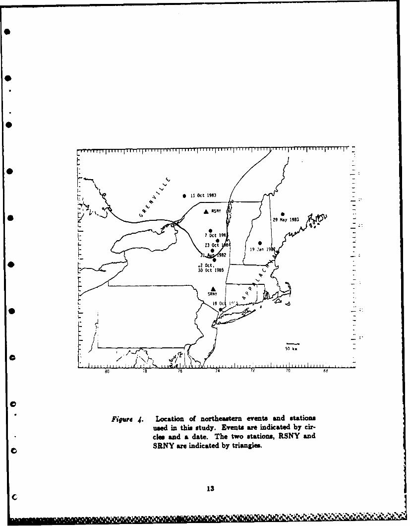
Figure 4. Location of northeastern events and stations used in this study ........ 13

Figure 5. Two velocity models and resulting synthetic seismoams ................ 17

0Figure 6. Two fault plane solutions and resulting synthetic seismograms .......... 18

Figure 7. Location of OSS-IV and the Kuril/Kamchatka events used in thisstudy .. . ................................................ 21

Figure 8. Seism recorded at RSNY of the January 19, 1982, NewHampshire earthquake, A - 267 km .................................................. 24

Figure 9. Synthetic seismograms calculated for a suite of depths ..................... 25

Figure 10. Same as Figure 9 except the real data are included in the depthsection at a depth of about 9 km ....................................................... 26

Figure 11. Like Figure 10 except notice that the real data are plotted at a -

depth of about 4.5 km . ...................................................................... 27

Figure 12. Adaptive polarization of state-filtered seismogram recorded atR SN Y . ............................................................................................... 28

Readout Associates, Inc. iv March 1967

ATAC Final Report

Figure 13. Like Figu 10 and 11 except the real data are plotted at a depthof 6 km in the depth section .............................................................. 30

Figure 14. Vertical, radial, and tran se components of motion for theAugust 31, 1982, Adirondack earthquake as recorded at stationRSNY, A-IS kn .k ............................................................................ 32

Figure 15. Synthet seismorm depth section for the Adirondackearthquake .............................................. 33

Figure 16. Best At of the RSNY data to the synthetics for the Adirondackearthquake (7 kin) . ............................................................................ 34

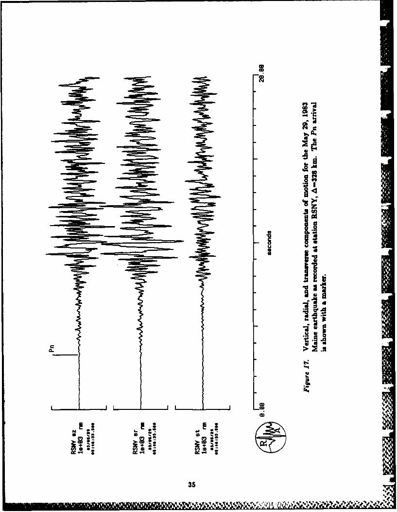
Figure 17. Vertical, radial, and transverse components of motion for the May29, 1963 Maine earthquake as recorded at station RSNY, A-328km ........................................................ 35

Figure 18. Synthetic seismogram depth section for the Maine earthquakeA m328 km . ......................................................................................... 36

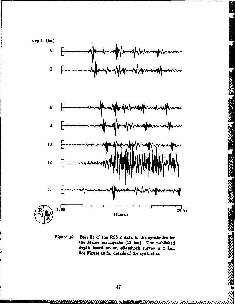
Figure 19. Best fit of the RSNY dits ot the synthetics for the Maineearthquake (12 km ) . ........................................................................... 37

Figure 20. Vertical, radial, and transverse components of motion for theOctober 7, 1983, Goodnow ernthquake as recorded at stationRSNY, A-69 km . .............................................................................. 39

Figure 21. Synthetic seimogram depth section for the Goodnow earthquake.40

Figure 22. Best fit of the RSNY data to the synthetics for the Goodnowearthquake (10 km ) . ........................................................................... 41

Figure 23. Vertical, radial, and transverse components of motion for theOctober 11, 1983, Ontario earthquake as recorded at station RSNY,A - 123 km . ........................................................................................ 43

Figure 24. Synthetic seismogram depth section for the Ontario earthquake ........ 44

Redout Associate, Inc. v March 1987

AFTAC Fizal Report

Figure 25. Beat Atof the RSYdata to thesyntheticsfor theOntarioearthquake (13 kin)......................................................... 45

Figure 26. Vertical-component synthetic sesormdepth section for theOctober 23, 1984, earthquake with the RSNY vertical trace plottedat12 km depth.............................................................. 469

Figure 27. Radial-component synthetic sesormdepth section for theOctober 23, 1964, earthquake with the RSNY radial trace plottedat 12 km depth.............................................................. 47

Figure 28. Vertical-comoponent synthetic seismogram depth section for theOctober 23, 1964, earthquake with the RSNY vertical trace plottedat 12 km. depth.............................................................. 48

Figure 29. Radial-component synthetic seLa depth section for theOctober 23, 1964, earthquake with the RSNY radial trace plottedat 12 km. depth ............................................................... 49

Figure 30. Vertical-component synthetic sismogrI depth section for theOctober 23, 1964, earthquake with the SRNY vertical trace plottedat12 km depth................................................................5o

Figure 31. Radial-component synthetic sesormdepth section for theOctober 23, 1964, earthquake with the SRNY radial trace plottedat12 km depth.............................................................. 51

Figure 32. High-pam filtered 3-component data (> 0.5 Hs)A. Quarry blast near Amsterdam, NY, at SRNY.B. Earthquake near Amsterdam, NY, at sRNY ......................... 53

Figure 33. 1 - 5 Hzs data. Top three traces are the blast, vertical, radial, andtransverse components; bottom three are the earthquake ............... 54

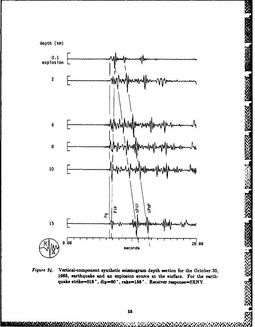
Figure 34. Vertical-component synthetic sioai depth section for theOctober 30, 1965, earthquake and an explosion source at thesurface .......................................................................... 55

Figure 35. Vertical-component synthetic depth sections compared to state-filtered si -ogram recorded at SRNY.................................... 56

Readout Aasoeiates, Ine. vi March 1967

WAR Au U I a m~Ua

AFTAC Final Report

Figure 36. Ardsley, NY, main shock and afterhock ........................................... 59

Figure 37. Deconvolution of the Ardsley main shock by its largest aftershock.61

Figure 38. Fault geometry for the Ardsley earthquake ........................................ 62

Figure 39. Vertical component synthetic seismograms for the Ardsley, NY,aftershock and data at station SRNY, A-100 km ............................. 65

0Figure 40. Ray paths of the primary and depth phases. ..................................... 66

Figure 41. Vertical component synthetic seismograms for the Ardsley, NY,main shock at station RSNY, A-400 km ......................... 67

Figure 42. 120 seconds of unfiltered data from OSS-IV for event KI, A-86170

Figure 43. State filtered (sf) and band-pas filtered (bp) P-wave data for eventK1, A-861 km ........................................... 71

Figure 44. Adaptive polarization analysis of event K1, A-861 km .................... 72

Figure 45. State filtered (sf) and band-pass filtered (bp) P-wave data for eventK3, A- 1157 km. ................................................................... ........ 73

Figure 46. State filtered (sf) and band-pas filtered (bp) P-wave data for eventK4, A - M k7. ................................................................................. 74

Figure 47. State filtered (sio) and band-ps filtered (bp) P-wave data for eventKS, A-668 km. ........................................... 75

Figure 48. State filtered (sf) and band-pan filtered (bp) P-wave data for eventK6, 4-948 km ............................................ 76

Figure 49. State filtered (st) and band-pam filtered (bp) P-wave data for eventK 7, 4-949 km . ................................................................................. 77

Rondout Associateu, Inc. vii March 1987

AJTAC PimaI Report

Figure 50. State filtered (an and band-pas filtered (bp) P-wave data for eventKS, 8-946 km .................................................................................... 78

Figure 51. State filtered (o) and band-pass filtered (bp) P-wave data for eventK10, A-918 km ................................................................................ 79

Figure 52. State filtered (in and band-pan filtered (bp) P-wave data for eventK11, A-574 km ................................................................................. 80

Figure 53. State filtered (of) and band-pmw filtered (bp) P-wave data for eventK 12, A -795 km .................................................................................. 81

Figure 54. State filtered (f) and band-ps filtered (bp) P-wave data for eventK14, A-753 km .................................................................................. 82

Figure 55. State filtered (of) and band-ps filtered (bp) P-wave data for eventKIS, 4-1260 km ............................................................................... 83

Figure 56. State filtered (af and band-ps filtered (bp) P-wave data for eventK 16, A -797 km . ................................................................................ 84

Figure 57. State filtered (al) and band-pmw filtered (bp) P-wave data for eventK 18, A -788 km .................................................................................. 85

Figure 58. State filtered (so and band-pus filtered (bp) P-wave data for eventK19, A-1307 km .............................................................................. 86

Figure 59. State filtered (i) and band-pmn filtered (bp) P-wave data for eventK20, A-1291 km ............................................................................... 87

Rendout Assocate", Ine. it March 1987

APTAC Final Report

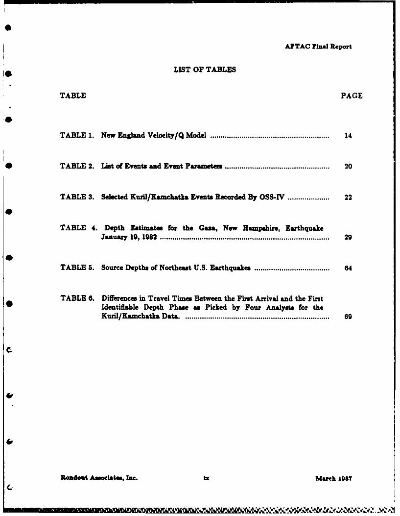
LIST OF TABLES

TABLE PAGE

TABLE 1. New England Velocity/Q Model ........................................................ 14

TABLE 2. List of Events and Event Parameters .................................................. 20

TABLE 3. Selected Kurl/Kamchatka Events Recorded By OSS-IV .................... 22

TABLE 4. Depth Estimates for the Gaza, New Hampshire, EarthquakeJanuary 19, 1982 ................................................................................. 29

TABLE 5. Source Depths of Northeast U.S. Earthquakes .................................... 64

TABLE 6. Differences in Travel Times Between the First Arrival and the FirstIdentifiable Depth Phase as Picked by Four Analysts for theKuril/Kamchatka Data . ..................................................................... 69

Roadout Associates, I=e. ix March 1987

C

APTAC Final Report

(THIS PAGE INTENTIONALLY LEFT BLANK)

Rondout Amaoclates, Inc. x March 1987

AJTAC Ilna Report

SECTION I

INTRODUCTION

The purpose of the research presented in this document is to refine our ability todiscriminate between nuclear explosions and earthquakes based on the depth of an eventdetermined from local and regional phases. If the depths of seismic events can be deter-mined accurately, many events can be eliminated as potential nuclear explosions basedon the practical limit of nuclear explosion burial depth. This discriminant has been usedfor many years at teleseismic distances. The higher frequency data obtained at local andregional distances improves the depth resolution of the method and thus the minimumdepth at which the discriminant may be applied. In addition, smaller events notrecorded at teleseismic distances may be seen at regional and/or local distances.

Our approach to this problem has been to improve phase identification and pickingabilities of depth phases pP and sP through filtering and three-component polarizationmethods. These methods are applied first to data from a set of earthquakes located inthe northeastern United States and adjacent Canada. The area of study was chosen forseveral reasons:(1) the large majority of events in this area occur at depths less than 15 km so that a

data set of shallow events is readily available,(2) the geology and tectonic setting of the area is well known and similar to that found

in the Soviet Union,(3) the depths of the events in the area of study are fairly well known from network

studies and aftershock surveys, and

(4) there are two broad-band three-component digital seismic stations in the vicinity:RSNY and SRNY. RSNY, part of the Regional Seismic Test Network (RSTN), isin northern New York and SRNY, operated by Rondout Associates, is insoutheastern New York.Having refined the techniques for depth determination in the well known region of

the northeastern U.S., the methods were applied to a set of data obtained from theOcean Sub-bottom Seismometer (OSS) installed off the Kuril trench in the north PacificOcean. Several events from the Kamchatka peninsula and the Kuril Islands were stu-died.

The most difficult problem associated with depth determination at local andregional distances using depth phases is identification. As the depth phases are usuallyburied in the coda, data processing plays a key role in identifying and picking them.Band-pam filtering and three-component polarization state filtering methods are used onthe data in an attempt to isolate the depth phases and adaptive polarization analysis isused to help identify them.

Once the depth phases have been correctly identified and picked, the depth can bedetermined accurately if the source region velocity structure is known. However,

Rondout Associates, Inc. 1 March 1987

- ~' vMN .

AFTAC lnd Iaport

misidentification of phases can lead to severe errors in the depth estimates. To assess thepotential depth errors resulting from these problems, synthetic seismogram depth sec-tions have been generated for each of the events in the northeastern U.S. to compare tothe identification and time picks made from the data. Of course, the depth of the eventis not the only factor contributing to the character of the depth section; the velocity-depth structure used and the focal mechanism are also very important to the overallcharacter of the section.

In the sections that follow, we briefly describe the analysis methods used on thedata to isolate depth phases, review the set of earthquakes that we have selected forstudy, and show detailed analyses of the earthquakes.

Radout Amoates, Inc. March 1987

A"TAC Final Report

SECTION II

EVENT DEPTH DETERMINATION

In this report we describe a method of depth determination that involves enhancingthe suspected depth phases at the beginning of the P coda using advanced polarizationmethods on three-component broad-band data. Single station techniques wereemphasized as, in a realistic test ban monitoring situation, it is likely that only one sta-tion will record many of the suspect events. The particular techniques used to enhancethe depth phases were adaptive polarization analysis, a method that adaptively rotatesthe horizontal components to the direction of maximum and minimum energy propaga-tion, and polarization state filtering (Samson and Osen, 1981), an adaptive frequencyfiltering technique that passes only those frequencies in a specified polarization state (e.g.rectilinear). These techniques succeufuly enhance polarized energy relative to the scat-tered component of the coda, which typically complicates the interpretation of local andregional s We note, however, that our research has concentrated primarilyon events with signal-to-noise ratios of one or better, and studies on the effectiveness ofthe polarization state filter have shown that its effectiveness deteriorates below this level.Therefore, if depth phases are to be used to determine depth on very small magnitudeevents, then either better methods of enhancing the depth phases must be found orreceiver sites must have low noise characteristics.

The next phase of the proceming scheme is to identify the individual depth phaseseither through experience, synthetic seismogram comparison, or some other method.Because the depth phases all have the same phase velocity and polarization characteris-tics, identification of the phases cannot be made on these parameters alone. Additionalinformation such as relative arrival times and amplitudes must be used. Whateverscheme is used to identify the arrivals, it is generally assumed that the source is a simplepoint mechanism within the frequency band being studied. For events at local andregional distances, this assumption is not always valid.

Polarization State FilteringPolarization analysis of a three-component wavefleld is used to determine the vector

particle motion characteristics such as the degree of polarization, direction of propaga-tion and ellipticity. This information can then be used to design filters that emphasizeor eliminate waves having specific polarization properties. In seismology, this methodhas been applied to analyze and filter waves coming from certain directions, or havingrectilinear or elliptical particle motion, and to discriminate against isotropic noise (Sut-ton and Pomeroy, 1963; White, 1964; Archambeau et al., 1965).

Polarized arrivals can be enhanced, their wave type identified, and their direction ofpropagation, as well a their phase velocity for body waves and ellipticity for Rayleighwaves, determined. This information can then be used for phase identification, epicen-tral location, source depth determination, earth structure studies, ...etc. Data filtered for

Roadout Amoelat., Je. z March 1987 Ie

.:9

ArTAC itro Report

polarized signal are more amenable to comparison with synthetic seismograms, providinga better determination of relevant parameters.

The polarization state method was proposed by Samson (1977) for the analysis andfiltering of sismogrms . It makes use of the spectral matrix, which is the frequencydomain equivalent of the crow-correlation matrix of the data, smoothed over a frequencywindow. Various spectral estimator can be obtained from the spectral matrix, such asthe degree of polarization, the degree of rectilinear polarization, a detector for signal in aspecific "pure state" (i.e. completely polarized) or with specific polarization characteris-tics. Such estimators can then be used to filter the data in order to discriminate againstunpolarized noise or to enhance signal in some specific polarization state (Samson andOlson, 1981). Since the polarization characteristics of seismograms continuously changewith time, such filters have to be data-adaptive: a sliding time window of data isanalyzed and a filter is specifically designed for that window. Polarization properties aredetermined and used not only as a function of time, but also as a function of frequency,since the procesing is done in the frequency domain. This is an advantage that methodswhich operate purely in the time domain do not have.

To enhance depth phases pP and #P we take advantage of the three-componentpolarization state filter's ability to pass frequencies that contain rectilinearly polarizedmotion and rqject frequencies that do not.

After the data have been state filtered for rectilinear motion, they are procemedwith an adaptive polarization method. The horizontal components are adaptivelyrotated to the time varying radial and transverse directions and the time variableazimuth and apparent angle of incidence are given. This process helps in theidentification of phases. Also, the synthetic seismogram components are the radial andvertical so rotating the horizontal data to the adaptive radial and transverse componentsfacilitates comparison.

Adaptive Polarization AnalysisIn the Adaptive Polarization Analysis method developed at RAI, the horizontal

components are adaptively rotated to the time varying radial and transverse directionsand the time variable azimuth and apparent angle of incidence are given. This proceshelps in the identification of phases. Below we present the theory behind this methodassuming rectilinear motion at a constant azimuth and angle of incidence. Later in thediscussion, we will consider simultaneous arrivals from different directions.

We seek to determine the azimuth and angle of incidence over a small time window;one that is at least as long as one or two cycles of the predominant frequency. Theazimuth is determined by examining the zero lag crom covariance between the two hor-izontal components as a function of azimuth angle. One of the angles at which this func-tion is zero is the azimuth of the predominant particle motion. The horizontal com-ponents of motion as functions of the north (N) and east (E) horisontais and theazimuth (0) are written:

Rondout Associates, Inc. 4 March 1987

ANTAC Nina Report

Hl(t) - N(t)coul + E(t)sint

H2(t) - 1(t)cos* - N(t)sin* (1)

and, the croa-covariance between Hi and H. at zero lag is:

Sccv, = - E (t +iAt) f(t +iAt) (2)n- 0

where 11(t) - H(t) - , is the mean value of H(t) over the interval, and At is thesampling interval. In terms of 1W and 1:

ccvo(O) = acoS2D + bsin2O (3)

where

4 = -- FN(t + iAt)z(t + iAt)n'- 0

1 2 -b -- E[ (t + iAt) - !e(t + iAt)]/2

n'-0

Solving for 0 at ccv0 0 - 0:

* - tan 1 (-a/b)/2 (4)

The azimuth 0 obtained from (4) will be between -45 * and 450 and could representany one of four directions; the direction of particle motion, its supplement, its transverse,or the transverse supplement. Without using the vertical component, the directionobtained from (4) can be determined with a 180" ambiguity by examining the behaviorof (3). The zero lag cron-covariance as a function of azimuth given by (3) is a sinusoid.Suppose that the 0 determined from (4) aligns the H2 component with the direction ofmaximum particle motion. Increasing this 0 in (3) will place the direction of particlemotion between the Hi and H3 components and the value of ccv0 will increase. Con-versely, if H1 is aligned with the direction of particle motion by (4) then increasing 0 in(3) will decrease ccv0 . Thus, when the slope of the sinusoid given by (3) at the azimuthdetermined in (4) is positive, then 0 is transverse to the direction of particle motion (orits supplement) and when the slope of the sinusoid given by (3) at the azimuth deter-mined in (4) is negative, then 0 is the direction of particle motion (or its supplement).Rather than computing the slope from the derivative of (3) with respect to 0, we can find

oits sign by examinin (3) at -, 0 where ccv0 (0) = a, If the signs of a and the 0 foundfrom (4) are similar (i.e. both have the same sign), then the slope is negative and I is thedirection of particle motion or its supplement. if the signs are dissimilar, then the slopeis positive and the direction of particle motion is at either I + 90' or 0 - 90 . Thedirection of particle motion can be either longitudinal or transverse to the propagationdirection depending on whether the particle motion is P/SV or SH. if the azimuth fromthe event to the station is known, then particle motion between ± 45" of that azimuth

Roadoat Associates, I. March 1987C

'r 'e ,' r "f,' , ,, 'r~m 't~n' , Ow '' ' '

AJTAC Pinl Report

can be considered radial and between 450 and 135 * or -45 * and -135 * can be con-sidered transverse. The azimuth obtained from (4) together with the assumed azimuth tothe event can be used to rotate the horizontal components to the radial and transversedirections at the center of the window. The window is then advanced one sample andthe process repeated. The radial and transverse traces separate the P/SV/Rayleighmotion from the SE/Love motion.

The apparent angle of incidence is calculated in much the same manner as theazimuth. For this meaurement, the adapted radial and vertical components are used asthe orthogonal components from which the angle of incidence is determined. The dis-tinctive particle motions of P, SV, and Rayleigh waves are distinguished using theapparent angle of incidence. P motion gives a positive value, SV a negative one andRayleigh a rotating angle of incidence.

An estimate of the relative accuracy of the azimuth and angle of incidence measure-ments is obtained through the maximum value of the zero lag crom-correlation function.At its maximum value, where the predominant direction of motion bisects H1 and H.,the sero lag crom-correlation function (ccf*(# + 45 )) will be between 0 and 1, inclusive.A large value is indicative of strong rectilinear motion over the window and a smallvalue indicates the lack thereof. Where there is little or no rectilinear motion, confidencein the results obtained is also small and we expect the error to be close to 90. Con-versely, a large value for ccfo(# + 45 ') indicates strong rectilinear motion and shouldhave an error close to 00. This subjective error evaluation can be written:

error= 90(1 - ccf( + 45)). (5)

Error determined in this manner is not an absolute quantity but rather a relativemeasure of the accuracy of the value.

Because the method presented here relies on the determination of the predominantdirection of motion, the question arises; "What angle would be determined if twouncorrelated signals arrived at the station at the same time from different directions?".Let the two uncorrelated signals be x(t) and y(t) where the standard deviations of x andy are equal and define the north and east components of motion as

N(t) x(t) + ky(t)()E(t) - rx(t) + sy(t) (6)

j, k, r, and s are scaling factors that can be set to simulate any combination ofdirection and amplitude for x and y. Substituting the values for N and E in (6) intoequation (4)

t

Readout Associates, Inc. 6 March 1967

A1TAC Final Report

E[x + ky)(rx + my) _

2 1F((rx +sly +rkm- jY - ky -2jkxy1/

Because x and y are not correlated, the xy terms tend to zero as the length of theseries get. large. Rewriting (7) eliminating thee term.

( - r 2)x + (ks _)

2~ 1 E2(r ?x 2 + W2 sm- 1 (8)

Equation (8) may be used to predict 9 for two time series passing a station atdifferent azimuths. The wort cae occurs when the two wavetrains are traveling atazimuths 450 apart, for when one of the signals is showing no correlation at its azimuth,the other will be at a maximum. If the two signals are orthogonal, then the properazimuth would be chosen.

The above analysis is valid only in the case that the two signals are not coherent.When the two signals are perfectly coherent then the azimuth determined will be that ofthe vector sum of the two signals. Partial coherency would result in some combinationof the completely non-coherent result and the perfectly coherent result.

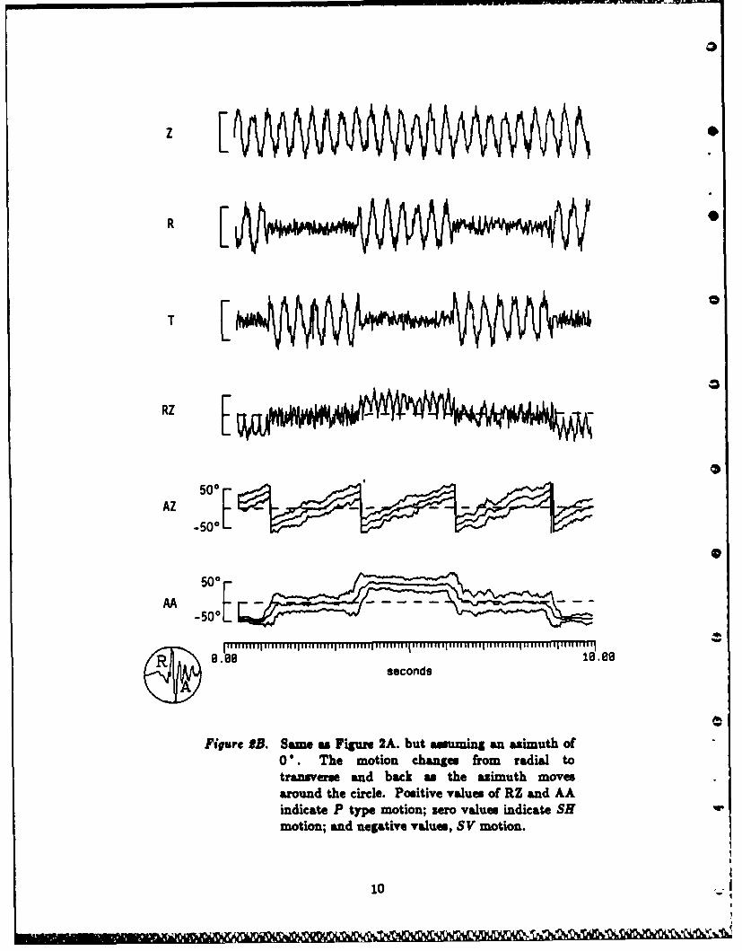
In Figure 1, we show synthetic vertical and horizontal components to be used as theinput to the polarization program. The modulated arrivals on the horizontal com-ponents represent a constant amplitude signal that rotates smoothly in azimuth. A con-stant amplitude vertical component maintains an unchanging angle of incidence. Theresults of processing this data with the polarization program, assuming that the signalcontains longitudinal motion exclusively, are shown in Figure 2A. There are six outputtraces; the vertical, adapted radial, and adapted transverse components of motion, theproduct of the radial and vertical traces, and the azimuth and apparent angle ofincidence trace, plotted with error bars. The radial trace exhibits a constant amplitudeand the transverse component shows very little motion at all. Thus, the radial followsthe predominant direction of motion. In the can of a short duration arrival, the RZtrace would help to identify the &st arrival and its direction but in this cow, where thesignal is continuous, RZ has little use. The azimuth trace tracks the motion of the rotat-ing arrival quite well and shows very little erros. The same is true of the apparent angleof incidence trace where there is no change throughout the duration of the analysis.When a propagation direction is assumed in the polarization program (Figure 2b), theparticle motion jumps between the radial and transverse components as the azimuthrotates from one direction to the other. The RZ and apparent angle of incidence traceshelp to identify the type of motion. When positive, the motion is P type; when nega-tive, SV; and when sero, SH. Rayleigh waves produce a rotation in the RZ and angle of

Randout Associate, hIe. March 1987

tvh

z

N

0

/RJI 0.90 19.0seconds

Figme 1. Vetical, North-South, and East- West com-ponents of motion for a signal sweeping 360 * ofasimuth plus noise.

I. Z

* R [

* T

RZ E100

A.10001I

50

500 1.~

I ........1 W.1 I It111111111 If If1111 It11 1111111111 11 11 t11 5111111 f111111111 11 f1111 1111 111111If111115111

R. 018 19.99seconds

* Figure M. Adaptive polarization analysis of the data inFigure 1 assuming no azimuth. Z-vertical;R-radial; T-transverue; RZ-sign (RZ) vlff;AZ-azimuth with relative error bars; AA-angleof incidence with error bars. The radial tracetracks the direction of particle motion aroundthe circle.

0 9

Z

T [0

RZ E0AZ 500r

_Z 50I

50 0 rAA -*

19.0 01111 10.0lll11811 11818 seconds100

Figure OR. Same as Figure 2A. but uusuming an azimuth of0". The motion change. from radial totransverse and back as the azimuth move.around the circle. Pouitive value. of RZ and AAindicate P type motion; zero value, indicate SHmotion; and negative value., SV motion.

10 -

AFTAC Final Report

incidence traces. Note that the azimuth trace jumps from +45 " to -45 as theassumed phase changes from SV to SH to P etc. This occurs because the propagationazimuth for SH motion is set to be + or - 90 " from the particle motion.

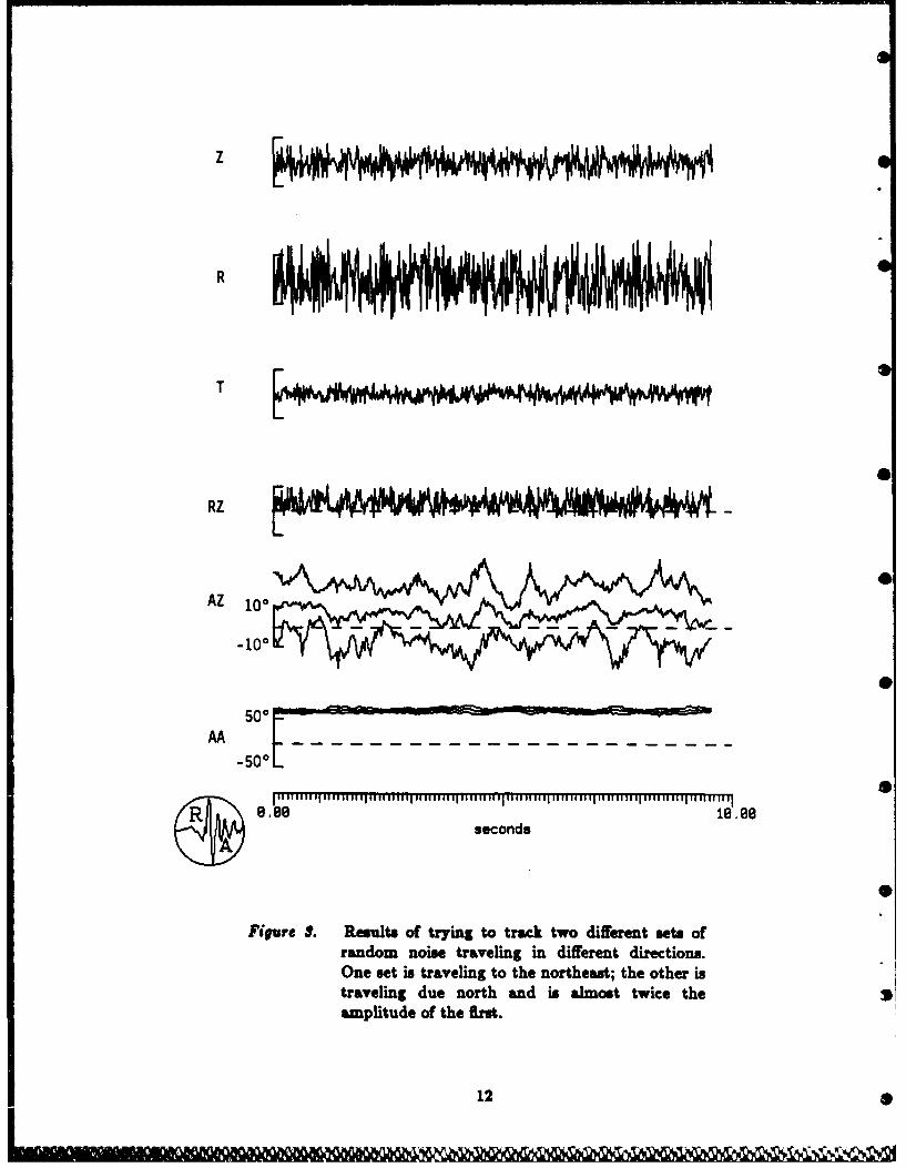
For the second example, two independent samples of random noise were combinedon the N, E and Z components of motion to simulate one set of arrivak traveling at 0azimuth, 72' angle of incidence with an amplitude of 1000 and another set of arrivalstraveling N45 E, 55" angle of incidence and amplitude 548 (amplitudes are relative).In terms of the independent non-coherent time series x(t) and y(t):

N(t) =3.0x(t) +y(t)

E(t)=y(t) (9)

Z(t) =x(t) +y(t)

Using these numbers in equation (8), we obtain values of 6' for the azimuth and67" for the angle of incidence (assuming an azimuth of 6" for the radial trace). Theresults of the polarization analysis are shown in Figure 3. The azimuth trace is centeredabout 6 over the length of the trace in excellent agreement with the theory. Error forthe azimuth is large and is due to the fact that the two arrival sets are traveling atazimuths 45 apart; the worst possible case. For the apparent angle of incidence, themeasured value of 67" is also in excellent agreement with theory and in this case theerror is very small. The small error arises because the two arrival groups are traveling ata similar angle of incidence in the vertical plane at 6" azimuth.

The adaptive polarization analysis program is a useful tool for locating earthquakeswhen only a single three-component data set is available. The azimuth from the initialP-wave, where presumably the error will be smallest and no conflicting arrivals arepresent, combined with the distance obtained from the S-P time gives a fairly accuratelocation.

Synthetic Seismograms

The synthetic seismograms were computed using the locked mode method (Harvey,1981) at frequencies from 0 to 5 Hz. Regional geology in the Northeast required thattwo different velocity/attenuation models be used for the computation; a New Englandmodel for the events in New England and southern New York, and a Grenville model forevents within the Grenville province (Figure 4, Table 1). The New England velocitymodel was derived by Taylor et at, (1980) using regional travel times of P and S wavesrecorded across the Northeastern United States Seismic Network operated by severalacademic, governmental and private institutions in the northeast. The Grenville modelwas from unpublished refraction results. The frequency and depth dependent Q modelfor the New England model was adapted from work by Mitchell (1981) and a simple fre-quency dependent Q was used for the Grenville model. Although there are significantdifferences in the Q models, there is little effect on the synthetics because the frequenciesand ranges at which they are being computed are relatively small.

Readout Associates, Inc. 11 March 1987

Z

R

T

RZ

AZ100

5100

-500 - T

/RIA .i 9.00 10.00seconds

Figure S. Results of trying to track two different mets ofrandom noise traveling in different directions.One set is traveling to the northeast; the other istraveling due north and in almost twice theamplitude of the first.

12

ASSN

00

FFur 1. Joaino othatr vnsan d ttin

SRNYSRN arqniae ytinls

1 c "

ce

AFTAC 11.. Repot

Synthetics were computed for each event at several depths with the reported focalmechanism listed in Table 2. The instrument response was convolved with the synthet-ics for comparison to the data.

Station RSNY lies within the Grenville structure close to the boundary with theNew England Structure. While the travel paths to RSNY from New England eventsmust pas through both structures, the nmjority of the path is within the New England 0structure and so the New England structure is a good approximation to the true path.

Throughout this report, only the first 20 or so seconds of the synthetic depth sec-tions are shown as we wish to emphasize the characteristics of the depth phases withfocal mechanism, depth, range, and velocity model. Some of the phases are identified inthe synthetic sections with labeled lines. Reflections off of the 13 km discontinuity in theNew England model and the 4 km discontinuity in the Grenville model are indicatedwith an i (e.g. PiP). Mantle reflections are indicated by an m. The depth phasm arecharacterized by progresively later arrivals with increased depth and the primary phasesby either very little change in arrival time with depth for the direct arrivals or progres-sively earlier arrivals with increased depth. In some of the sections, the depth phasesdominate, while in others, the primary phases dominate. This is a function of thetheoretical radiation pattern predicted by the input focal mechanism. Because the inputvelocity structure will influence the take-off angle of each phase and hence its position onthe focal sphere, both focal mechanism and velocity model contribute to the relativeamplitudes of primary and depth phases.

TABLE I

New England Velocity/Q Model (Taylor et a.., 1980)

Thickness (kin) Vp (km/sec) VS (kin/sec) p (gm/cm3) Q Q0

2 6.0 3.5 2.5 O/5 250f0 213 6.1 3.6 2.6 500o.225 7.0 4.1 2.9 1000.2

8.1 4.7 3.2 3000/o._

Grenville Velocity/Q ModelThickness (kin) V (km/se) V (km/sec) (

4 6.1 3.5 2.5 1100+150 f 5Q'/o31 6.6 3.7 2.7

8.1 4.6 3.2

The succem of determining focal depth using depth phases and comparing them tosynthetics depends largely on:(1) good approximations of crustal velocity structure, and

Road ut Aisoelat4, laC. 14 March 1967

U .. . . . . . . .6 )

A"TAC Final Report

(2) recovery and correct identification of the phases in the data.

Here we use one earthquake to illustrate how the synthetic seismograms are affected by 2different velocity models and focal mechanisms.

The earthquake chosen is the Gaza, N.H., magnitude 4.5 event of January 19, 1982.Since the source is in the Appalachian Province and the receiver (RSNY) is in the Gren-ville Province (see Figure 4) we calculated separate synthetics using the two velocitymodels (Table 1) to test which is more appropriate.

Figure 5 shows radial and vertical components for the initial 15 seconds of the syn-thetic seismograms calculated for two velocity models. RSNY is the theoretical receiver,a distance of 267 km and an azimuth of 295 * from the New Hampshire source. Thevelocity models and Moho reflections are shown schematically for comparison. The focalmechanism is given by: strike - 280, dip - 750 and rake -11. The input focaldepths are comparable.

As expected, the prominent phases and their arrival times are different for the twodifferent velocity models. The Pn phase is nodal for the radiation pattern, despite smalldifferences in take-off angles for the two models. It is simply indicated at the appropri-ate arrival time. For the New England model, PmP is small relative to aPmP. Theyboth arrive before the intra-crustal reflections PiP and #PiP. For depths greater than 10kin, however, PiP arrives before aPmP. PiP and .PiP are sharp arrivals because of thelarge velocity contrast at 15 '-m in the crustal model. Vp increases from 6.1 km/sec to7.0 km/sec at this boundar)

For the Grenville model, Pg precedes the Moho reflections (for a source depth of 7kin). The amplitude of 8PmP relative to PmP is smaller for the Grenville model thanfor the New England model because the upgoing ePmP is crossing a fairly sharp internaldiscontinuity near the source while the downgoing PmP only croses this boundary once,near the receiver. In the case of New England structure, the sharp discontinuity is belowthe source, instead of above it. In addition, PmP is close to a nodal plane and smalldifferences in take-off angle, resulting from differences in the velocity structures, may becontributing to the difference in the amplitudes of PmP.

Even though the two velocity models produce strikingly different synthetic seismo-grams, it is important to note that for the depths and models shown, the time betweenthe arrivals of the downgoing and upgoing Moho reflections is the same. Thus, if onecan independently identify these two phases in the actual data, a match (ignoring abso-lute travel times) to the Grenville synthetic would suggest a depth of 7 km and a matchto the New England synthetic would suggest a depth of 6 km. Given this timedifference between the two arrivals, the choice of velocity model has had only a smalleffect on depth determination. If, however, one uses the computed phase travel times tohelp identify depth phases in the real data, the variation in travel time with velocitymodel could lead to misinterpretations of the real data.

Next, in Figure 6 we show 15 seconds of synthetics calculated for 2 different focalmechanisms. The mechanism shown at the bottom was determined from P-wave firstmotion data, mainly from the Northeast United States Seismic Network (Pulli et al.,

Roadout Associates, Inc. 15 March 1987

.6

APTAC Flb.l Report

1983). The mechanism at the top of the figure differ. mainly in the quadrants of dilata-tion and compresion. The azimuth to station RSNY is very close to a nodal plane inboth instances, so there is not a great difference in radiation pattern. Thus, the sameinitial phases appear on both sets of seismorams, but the amplitudes of these phases aredifferent. If theoretical radiation patterns can be used to predict actual phaes in thedata, then it will be helpful to have independently determined fault plane solutions.

I

0

0

Rtendout Assoolates, Inc. 16 March 1967

New England Mudel 0

1.1

SP7.0

A la0

NEW ENGLANDmodel

Pn PmP sPuI PIP sPIP

seconds 15 Go

Grenvl I Ie ModelI

Z-7 -PS 4

B PmP Pg

B~ 35

SRENYI LLEModel r AZ-71= ~ L . . . ...................... t

Pn PeAPP sPW

16seconds C

January 19, 1982, Am 267 KM., AzlMUth= 295.Figure S. Two velocity moadl. and resulting synthetic seuwogams.

A) New England Model, soumc depth-n km. Source-to-receiver Moho,reflections shwn schemtcally. 15 mands of radial and vertical com-ponent synthetics, with phases identified. PiP and sPiP are internalreflections at the 15 km boundary.B) Grenville model, source depth-7 km. Source-to-receiver Moho,reflections shown schematically. 15 seconds of radial and vertical com-ponent synthetics with phase identified.

17Ar 0-~ -r

Strike a0200, Dip 750, Rake = 110~

RL

Z-6an

PM. second 156

Figue6. rik Tw 280lt plan soluio, Rakdesutn syntheti

aetogrm..Fifenseconds ofterdaan

twodifferen t iu s o al ln olutions.Teaiuht

RSNismgs initen byaclnes o the faaul pane

solution, a lower hemisphere projection withcompreeional quadrants filled in.

AFTAC Flla/ Roport

SECTION III

DATA

In the northeastern United States and Ontario, Canada, eight local and regionalearthquakes and one quarry blast were selected for study. The events were chosen fortheir size, location, and availability of data. A list of these events is given in Table 2along with location, depth, magnitude, strike, dip, and rake of the focal mechanism, theregion (either New England or Grenville), and references for the focal parameters. Theevent and station locations are plotted in Figure 4, showing their spatial distribution.Many of the earthquakes in Table 2 have been studied by others and, for some, the focaldepths and focal mechanisms are well determined and will provide an excellent base forcomparison.

In addition to reviewing the literature, we examined phase data from local seismicnetworks originally used to invert for hypocentral location. In three caes the estimatederror on focal depth was so large that to use the reported depth would be misleading.For these we indicate (Table 2) an unknown depth.

Most of the data were recorded by RSNY, in northern New York, at 44.55" N,74.53 W. Several of the recent events were also recorded by SRNY, a very-broad-bandseismic station operated by Rondout Associates in Stone Ridge, New York, at 41.85" N,74.15" W. a

Data for the Kurl/Kamchatka portion of this study were recorded by the fourthOcean Sub-bottom Seismometer (OSS-IY) emplaced 380 m below the sea floor at thebottom of DSDP hole 581C (440 N, 160 E). The data spanned the period from Sep-tember 12 to November 16, 1982 and the events selected for study are listed in Table 3.The closest event to OSS-IV in 574 km away and the furthest 1307 km. The large dis-tances make the computation of synthetic seismograms using the locked mode methodunreasonable.

Crosstalk and skew problems hamper analyses of the OSS-lV data. The skew waseasily corrected but the amount of crostalk is difficult to judge. Theoretically thecrosstalk problem effects only the azimuth and apparent angle of incidence determina-tions and not the isolation of the depth phases needed for depth determination. Relativeamplitudes of the phases may not be correct, but the polarization state filter does notpreserve absolute amplitudes anyway, so the point is unimportant; it is only mentionedhere for the sake of completeness.

A map of the event locations in Table 3 and OSS-IV is given in Figure 7. Theevents were classified as being either excellent, good or bad for depth determinationbased on the signal-to-noise ratio and impulsiveness of the records. Recordings that wereemergent and unlikely to show clear depth phases without a great deal of processing wereclassified as bad. The excellent (*) and good (x) data seem to be associated with thedowngoing Pacific plate and the bad (o) data with the shallow events within the accre-tionary wedge of the Kamchatka peninsula. The number of events studied is too small

Rondout Assoclates, Inc. 19 March 1987IM

2c to0 ( C-

cc jLf P.. U 4 Lfl -4 00 -

cc M Unf) 4CV

w ~ ~ ~ ~ r. -nr . )4L&J 4-)JL

uiLn tz -0.0..e

.-- i Cfl 0% ('.1 0, in 0 (

ui 4- 4- ~ ~ ~ 0LL.

000

4,-.% Inr L % n ( m )- 0_ 4

0 41c-

.- -: . Nl m 00. g n q -Ir Ln qr 0'if 0 41 %O0 0 0O

ui 0 vU a,

Li- 4-'-oz. In._0

0~ ~~~ 0% 0--4- 0 ~,iIU"AJ CJ tv to to % o .

9.-- fu VI * . 01(a 1%. a)- 4.3 4%1 4s).4. . .

m = w w = -(D o 3 t. '4- 1m. 2 .~L % 7% 0% % 2% 0% u a 0C0 14S-S,

. . - -. -4 1-C '4- C- G J0 a)4 ()

0- S- U s0 = 00 m -

4.1

2.'0 .3

AITAC lb.] Repairt

to attach much significance to this observation; however, the results are easily explainedby the tectonic setting of the region. In general, energy that must pass through the tec-tonic boundary between the Asian and Pacific plates is attenuated much more than thatwhich has a travel path wholly in the Pacific plate.

TABLE 3

Selected Kuuil/Kainchatirs Events Recorded By OSS-IV

Event Date Time Lat Lon Depth m6b

TF T7U7KF 1:4:57.0 "45.3 1'T.i - - 6KIO 10/11/82 22:27:43.2 52.15 160.89 23 4.7 918KII 10/23/82 11:41:01.0 47.10 154.0 30 5.0 574Ki 09/21/82 -21:29:.44.9 51.63 158.66 40 4.8 861K4 10/03/82 14:05:39.0 47.1 153.5 120 4.7 605K12 10/23/82 23:19:25.5 50.96 158.10 40 4.6 795KIS 11/15/82 18:53:.06.8 50.93 158.18 42 4.5 1788K3 10/03/82 00:32:57.2 -54.28 161.37 33 4.8 1157K6 10/11/82 15:31:26.9 52.45 159.61 14 4.7 948K7 10/11/82 15:33:22.5 52.46 159.5 6 4.8 949K8 10/11/82 15:35:22.6 52.43 159.66 14 4.7 946K14 10/25/82 12:~06:47.3 -50.46 157.2 40 4.7 753K15 10/25/82 15:38:58.6 55.15 162.18 10 4.8 1260K16 11/13/82 19:58:46.0 50.95 157.69 - 4.7 797K19 11/15/82 19:18:17.1 54.84 166.52 4 5.1 1307K20 11/16/82 100:51:12.6 5 5.25 163.76 6 4.6 112911

A search was mae for data fr-om station MAJO in Mateashiro, Japan to aid in theKuril/Kamchatka study. Unfortunately, only long period data was available for theevents listed in Table 3.

Ruadout Amdeatmu, 1.m. 22 Mlarch 1987

APTAC Final Rhport

SECTION IV.

DATA ANALYSIS

In this section we show how we estimate source depths of the earthquakes presentedin the previous section. First, the northeast North American events are compared tosynthetic seismogram depth sections and a best-fit depth is selected. This is followed bya brief presentation of the Kuril/Kamchatka OSS data, which turns out to be ill-suitedfor depth determination.

New Hampshire, January 19, 1982It would be very difficult to compare the raw data recorded at RSNY to the syn-

thetic sinograms (compare the top of Figure 8 with the synthetics in Figure 9). Withthe polarization filtering, however, we have been able to recover polarized phases (bot-tom of Figure 8) that were all but lost in the P-coda of the unfiltered seismograms.After polarization filtering, we low-pase filter the data to remove frequencies greater than5 Hz, which are not modeld by the synthetics.

The following figures show comparisons of the vertical-component RSNY procemddata to the vertical-componnt synthetic depth section calculated for the New Englandmodel. Twenty seconds are shown. W,.began by inserting the data at a depth of about9 km (Figure 10). Thee are several arrivals in the data that match predicted arrivals.These are, in order, ProP, &ProP, the dual arrivals PiP and Pg, and finally an upgoingphase arriving toward the end of this time window. Clearly, the match is not perfect.Signal arrives in the data later than the appropriate time for *PiP, and, subsequentlyuntil the late phase (in the data, about 14 seconds after the initial P), there is not agood correlation between data and synthetics. A comparison of travel times for the firstarriving phase in the data and synthetics suggests that they may not be the same phase.The travel time of synthetic ProP at a source depth of 9 km (with the given input velo-city model) is 40.40 seconds, whereas the travel time of the first phase in the data is38.59 seconds. Allowing for uncertainties in the actual origin time of the earthquake andfor uncertainties in crustal structure, they could be the same phase. Uf, however, weassume that the origin time and velocity model are appropriate, we can match severalearly P-phases by aligning the data at a depth of approximately 4.5 km as illustrated inFigure 11. Since the real-data travel time is more appropriate for Pn, the first arrival isnow aligned with the predicted Ph arrival time (compare Figures 10 and 11). For thisshallower depth, the data conform to predicted arrival times for Pn,PmP,aPmP and forthe late up-going phase. Again, the correlation among all phases, real and synthetic, isnot perfect.

At this point, it is clear that a great deal depends on the correct identification of thearrivals in the data. In addition to travel times, the azimuth and apparent angles ofincidence can be used to help identify phases. In Figure 12 we show the results of an

Readout AMsoiate, Ine. 23 March 1987

z

N0

E

Sz

N

E

seconds

Figure 8. Seismograms recorded at RSNY of the January 19, 1982, New Hampshireearthquake, A-267 km. The top three traces are the vertical, north-south,and east-west compovmnts, unfiltered. The bottom three traces are the threecomponents after state-filtering for rectilinear particle motion.

24

depth (kmn)

0

2

6 7

8

10 * _ - - - - - -

Pn mP ip sPmP sPiP

15

R e. 6e 28.00

Figure 9. Synthetic seismograum calculated for a suite of depths. Source-January 19,1982, earthquake. Strike-280, Dip-75, Rake--il. Receiverresponse-RSNY short period (up). Azimuth-295. PiP is reflected withinthe crust, and PmP is reflected at the Moho.

25

depth (kin)

0

2

L0

6

8

data F

10 f

PP

15

8.8 28.88seconds

Figure 10. Same as Figure 9 except the real data uweincluded in the depth section at a depth of about

28

depth (kin)

0

2

dataAl

6

8

10

pip

Pn mpsPmP sPiP

15

0.80 20.00

Figure 11. Like Figure 10 except notice that the real dataare plotted at a depth of about 4.5 km. See textfor discuinion.

27I

Z0

R

RZ

0 0 00 0

o) 0 CD 0l

AZ

N I g I I I I I I

/RI~.\8.8 2.60 a 0 second

28-0seconds

WE 30uuu .rIu tO S

AFTAC Final Report

adaptive polarization analysis of the first 20 seconds of the same state-filtered seismo-grams that we have been comparing to the synthetics. The first three traces 'a the figureare the vertical, and the adaptive radial and transverse horizontal components. Thedirection of maximum signal strength as a function of time represented by the azimuthand apparent angle of incidence, is indicated (with error estimates) below the RZ pro-duct trace in Figure 12. The positive values for the product of the radial and verticalcomponents indicate that all phases shown are arriving at the receiver as P-waves.Adaptive polarization analysis of the synthetic seismograms (not shown here) indicatesthe same thing; thus, at the very least, we know that the last conversions were to P-waves for both the real and synthetic data.

Interestingly, we noted that the last arrival, which had matched a predicted phasein the synthetics at both the 4.5 and 9 km depth positions, is probably not even modeledby the synthetics. Though highly polarized and hence a prominent phase in the data, itis fourteen degrees off the correct azimuth from the source. Unlike the two other out-of-line azimuths (see Figure 12), the error estimate is small and does not allow enoughuncertainty to put it in line. Furthermore, this late phase is approaching the receiver ata shallower angle than any other arrival (see the angles of incidence), yet the late phasein the synthetic seismograms approaches the receiver at the steepest angle in the same 20second time window. A steep, late arrival would be consistent with a multiply-reflectedphase.

TABLE 4

Depth Estimates for theGaza, New Hampshire, Earthquake January 19, 1982

Depth Estimate (km) Method Reference

3 local network Pulli et a., 1983

3.5 teleseismic body Pulli et at., 1983wave modeling

9 relative relocations Brown and Ebel, 1985using aftershocks*

4-11 regional, surface Hermann, pers.wave modeling Communication

*Depth range of larger aftershocks recorded by portable instruments is2.7-4.7km.

In the data, the phase immediately preceeding the last phase (by almost 1 second) ismore consistent with the synthetics because it approaches at a steeper angle. Using thatinformation, a different match can be obtained by inserting the data at a depth of 6 km(Figure 13). Here, the first arrival is a predicted PmP and there are phases matching

Rondout Associates, Inc. 2g9 March 1967

depth (kin)

0

2

data

8

10 F

pipPmP p Si

Pg

15A

/RJI 0.00 20.00~ seconds

Figure 19. Like Figure. 10 and 11 except the real data areplotted at a depth of 6 km in the depth section.See text for discussion.

30

I .... .....

APTAC Final Report

the predicted ePmP and the dual arrival of Pg and PiP, as well as the late multiply-reflected phase. This interpretation, however, given the largest mismatch in travel times.

One can see that it is not easy to choose among the above interpretations , becauseseveral are possible yet none provides a perfect match. The difficulties of identifying andcorrelating phases from a single set of three-component data are well-illustrated by thisexample. Evidently, this particular earthquake is difficult to pin down as the range ofestimates for its focal depth is 3-11 kin, using a variety of approaches (see Table 4).

Adirondack Mountains, August 31, 1982

No depth has been reported in the literature for the 31 August, 1982, Adirondackevent. Its location is 156 km from RSNY at a station to event azimuth of 170'. Depthphases would be very difficult to identify if just the band pam filtered data rotated to thevertical, radial, and transverse directions of motion were examined (Figure 14, top). Inthis cue, the polarization state filter was used effectively to pass only rectilinear motionand help in the depth phase identification (Figure 14, bottom).

The synthetic seismogram depth section computed for this event exhibits a strong*PmP phase, well defined SmP, pSmP, and ePmS phases and a weak Pg phase (Figure15). The strike, dip, and rake for this event have not been published and a generic faultplane solution for this area based on other Adirondack events was used in the syntheticprogram. Thus, the relative amplitudes of the phases do not match the data (Figure16). The state filtered data trace in Figure 16 has been aligned with the synthetics inabsolute time. In other words, no movement of the data trace with respect to the syn-thetics along the time axis was allowed. With this constraint, the large first arrival inthe data trace is identified as the Pg arrival and the second arrival is the *PmP arrival.The small arrival at about 10 seconds on the data trace may be the pSmP arrival.

The best fit of the data to the synthetics is at 7 km depth. We note however, thatif amplitudes are ignored (as they should be in this cue) the At of the data to the syn-thetics is nearly as good for any depth between 7 and 13 km.

Maine, May 29, 1983The reported hypocenter of the Maine event is at 44.50 N, 70.41 W, at a depth of

2 km. This location is 328 km due east of RSNY, the largest distance to any of thenortheast U.S. events studied. The data are characterized by a small Pn phase arriving46 seconds after the rupture followed 5 seconds later by a rather large emergent Pg. Thecoda amplitude remains fairly constant from the Pg arrival to the Lg arrival 38 secondslater (Figure 17). Synthetic seismograms computed for this event show large amplitudesPmP, PiP and ePiP phases and several unidentified depth phases (Figure 18). Thecoda of the Pg arrival in the data is not well matched by the synthetics for a 2 kmsource depth. Of more importance is the mismatch of amplitudes of the ePmP arrival.The *PmP arrival in the data has the same small amplitude as the PmP arrival. Abetter fit of the data to the synthetics occurs at 12 km source depth (Figure 19). At this

Rondout Associates, Inc. 31 March 1987

ZQ

R

S RUL.

P-"FW--

40)4.

T IPA, I

seconds250

Figure 14. Vertical, radial, and transverse components ofmotion for the August 31, 1982, Adirondackearthquake as recorded at station RSNY, A-156km. Lower traces have been polarization statefiltered for rectilinear motion to enhance thedepth phases.

32

depth (km)

-I

2

5

7

10 F-L

0.00 25.008

R aloeseconds

Figure 15. Synthetic seismogram depth section for theAdirondack earthquake. A-156 kin,strike-173, dip-60", rake-110, station toevent asimuth-170.

33

depth (kin)

2

7

10

ueconds

Figure 16. Best fit of the RSNY data to the synthetics forthe Adirondack earthquake (7 kmn). There hasbeen no published depth for this event. See Fig-ure 15 for details of the synthetics.

34

c..m

-4

9

8."

0u

LcIL

ccC

+* +

CIa.

35

depth (kin)

0

2

4=6

8

10 L

9.0seconds200

Figure 18. Synthetic simpam depth section for theMaine earthquake A-328 kmn, strike-355,dip-52', rake-78, station to eventazimuth-g0'.

36

depth (kin)

0

2

6

8

10 F

12 F

15 F - - - -

999 29.06seconds

Figure 19. Best fit of the RSNY data to the synthetics forthe Maine earthquake (12 kin). The publisheddepth based on an~ aftershock survey is 2 km.See Figure 18 for details of the synthetics.

37

9

APTAC Plusa Report

depth the sPmP phase arrives in the Pg coda where the amplitudes are better matchedand the arrival times of the distinct phases in the data are modeled well by the synthet-ics. Regional network data from 36 stations placed the depth of this event at 1.8 km.Support is lent to this depth by an aftershock survey conducted shortly after the mainshock that obtained a well determined depth of 2.4 km for one of the aftershocks (Ebeland McCafrey, 1984).

Goodnow, New York, October 7, 1983The Goodnow sequence of earthquakes occurred in the central Adirondack moun-

tains of New York on October 7, 1983. Following the m, 5.3 main shock, there werenearly 100 aftershocks with magnitude 3.5 and lower that occurred over the next twomonths. Station RSNY, just 69 km from the event recorded the P-waves reliably butclipped in the Lg portion of the wavetrain. The strike, dip, and rake of the main shockfrom first motion data are 173", 60', and 110". Station RSNY is at an azimuth of162 * and lies close to the intersection of the two nodal planes of the main shock. Thus,the record character for synthetics at RSNY is sensitive to small changes in focalmechanism.

The data shown in Figure 20 have been rotated to the vertical, radial, andtransverse directions and has been band-pass filtered between .5 and 5 Hz for comparisonto the synthetics. Several distinct phases are evident in the data.

Figure 21 shows the synthetic seismogram depth section for this event. The Pgarrival, strong when the source is deep, weakens significanly with foci near to the sur-face. The predominant phases are the ePiP and the SmP which exhibit strong ampli-tudes throughout the section.

A match of the data to the synthetics is shown in Figure 22. The initial Pg arrivalin the data trace is about .5 seconds earlier than the same phase in the synthetic sectionand the second arrival is not matched at all by the synthetics. Beyond that however, theePeP, SecP, pPmP and StoP phases are all matched well for a source depth of 10 km.Despite the sensitivity of the synthetics to small changes in the focal mechanism at thisazimuth, the relative amplitudes of the phases are fairly well matched also.

Two depths have been reported for this event, one at 7 km * 1 and one at 14 km±5. The shallow depth is based on aftershocks and on teleseismic observations of the mainevent, while the deeper depth is based on local travel times. The depth determined herelies between these two estimates. range of depths.

The large size of the Goodnow event (mb = 5.3) raises the possibility of a complexsource function. If this were the case, the complexities could be falsely identified asdepth phases and an improper depth determined. At this point, we do not knowwhether or not source complexities have influenced the depth for the Goodnow event.

Rondout Associate@, Inc. 38 March 1987

RSNY sz[2e+94 rm

I3/16/0719116MS.100

RSNY sr

2.+84ru

~ jllilii ~ 111111111 1 1111111111111~ 1111111 i 11111 II i fI 1 111111111111

0.98 ~seconds1 .0

Figure 20. Vertical, radial, and transverse components ofmotion for the October 7, 1983, Goodnow earth-quake as recorded at station RSNY, A4m89 km.

39

depth (km)

0

20

5

7

10

13

16

Vill .00 10.00

seconds

Figure 21. Synthetic seismogram depth section for theGoodnow earthquake. A-69 kin, strike-173,dip-60", rake-110", station to eventaimuth-163.

40 "

depth (kin)

0

2

5 0

7

data [

13A

16

/Ra.\00 10.00seconds

Figure SO. Best fit of the RSNY data to the synthetics forthe Goodnow earthquake (10 kin). The pub-liuhed depths range between 7 and 12 km. SeeFigure 21 for details of the synthetics.

41

AFTAC Final Report

Ontario, October 11, 1983The Ontario event occurred 123 km from station RSNY. It was a magnitude 4.2

event and had a reported depth of 15 km. Although the travel path between the eventand RSNY was wholly within the Grenville province (Figure 4), distinct phase aredifficult to identify in the data. Figure 23 shows the data rotated to the vertical, radial,and transverse directions. From the initial Pg arrival, the coda gradually increases inamplitude for the next 4 seconds.

Synthetic seismograms for this event (Figure 24) have a small Pg phase followed bya large amplitude PmP phases a few seconds later. Well into the coda there is a welldefined set of arrivals consisting of the SmP, PnS, pSmP, and oPmS phases

The fit of the data to the synthetics is poor (Figure 25). Neither the arrival timesnor the amplitude characteristics are matched. The depth that we have assigned to thisevent (14 kin) is based primarily upon the spacing of the (presumed) Pg and PmPphases.

Adirondack, New York, October 23, 1984On October 23, 1984, a magnitude 3.4 earthquake occurred in the southwestern

Adirondacks, near Johnsburg, New York. Because it was recorded by RSNY and SRNY,it afforded us the chance to model seismograms at two different receivers and thusincrease our confidence in the interpretations. We estimate a source depth of 12 km anda strike, dip, and rake of 353", 60", and 17 * for this earthquake based on the resultsdescribed below. Neither the depth nor the fault plane solution could be determined bylocal network data, though many stations recorded the event and its epicentral locationis fairly well constrained with an azimuthal gap of 43. The nearest network station,however, is 52 km from the source.

Synthetics to both RSNY and SRNY were calculated with the Adirondack velocitymodel. Initially, we tried the fault-plane solution of the Goodnow earthquake because itis well constrained and is similar to many other Adirondack solutions (e.g. Yang andAggarwal, 1981). Resulting vertical and radial synthetic depth sections are shown inFigures 26 and 27 along with RSNY band-pass filtered data plotted at a depth of 12 km.The data and synthetics, though aligned at the same time with respect to the origintime, do not look much alike. The lack of fit between data and synthetics, particularlyfor the relative amplitudes of different phases, suggests that the fault plane solution andhence radiation pattern of the synthetics is incorrect. A much better match is achievedusing a different fault plane solution of strike - 353 *, dip - 60 ', rake - 17 (Figures28 through 31). This mechanism has a greater strike-slip component and is not unlikeseveral previously determined Adirondack mechanisms (Schlesinger - Miller, et al.,1983). In Figures 28 and 29 RSNY vertical and radial seismograms are again plotted ata depth of 12 km where the arrival times and relative amplitudes, especially of PmP and*PmP, are well modeled by the synthetics. Furthermore, the polarity of the 3-cyclewaveform, ePmP, is opposite that of PrnP on both data and synthetics. Pg is nearlynodal for the theoretical seismograms and, in fact, no signal above noise was detected on

Rondout Associates, Inc. 42 March 1957

RSP4Y sz1e+83 rn

03/10/11

R1W srse

1.93 rn43110/11

RSNY st19+83 run$3/10/11

04, 111126Sa

R.4A. seconds

Figure RS. VerticaJ, radial, and transmverse components ofmotion for the October 11, 1983, Ontario earth-quake as recorded at station RSNY, A-123 km.

43

depth (kin)

00

5

7

10

13

seconds

Figure d4. Synthetic seismogram depth section for theOntario earthquake. A-123 kmn, strike-71,

B4

I ' ~ '

depth (kmi)

5

7

10

13

16

8.90 15.00

Figure *5. Best fit of the RSNY data to the synthetics forthe Ontario earthquake (13 kin). The publisheddepth for this event is 15 km. See Fire 24 fordetails of the synthetics.

45

depth (kin)

dataRSNY Z

13

R.6 28.00seconds

Figure 96. Vertical-component synthetic seianogram depth section for the October 23,1964, earthquake with the RSNY vertical trace plotted at 12 km depth.

Synthetics are low-pas filtered fr-om 3 Hz. Data are band-pas filtered, 1-3Hs. Strike-173*, dip-60', rake-1llO, A-115 kmn, asimuth-336'.Receiver response-RSNY short period.

46

depth (kin)

5

10

dataRSNY R

13

16

seconds

Figure 27. Radial-component mynthetic ieumgam depth section for the October 23,1984, earthquake with the RSNY radial trace plotted at 12 km depth. Syn-thetics are low-pms filtered from 3 Hz. Data are band-pms filtered, 1-3 Hz.Strike-173', dip-60', rake-1 0 , A-n115 kin, azimuth-i33C'. Receiverresponse-RSNY short period.

47

depth (kin)

5E

100

R 0.08 seconds200

Figure 18. Vertical-component synthetic seimmogram depth section for the October 23,1984, earthquake with the RSNY vertical trace plotted at 12 km depth.Synthetics are low-pmw filtered from 3 Hz. Data are band-pms filtered, 1-3Hz. Strike-353', dip-mOO, rake-17*, A-115 kin, azmuth-336'.Receiver response-RSNY short period.

48

depth (kin)

10

dataRSNY R

I I I I I I I I I I -T I I I i I

8.0 seconds 29.8

Figure 29. Radial-component synthetic seismogram depth section for the October 23,19U4, earthquake with the RSNY radial trace plotted at 12 km depth. Syn-thetics are low-pms filtered from 3 Hz. Data are band-pmn filtered, 1-3 Hz.Stuike-353', dip-GO0*, rak-17*, A-115 kmn, azimuth-336'. Receiverrespomme-RSNY short period.

49

........... .........

depth (kin)

5

7

0

10

dataSRNY Z

13

R 0.00 20.00seconds

Figure SO. Vertical-component synthetic seienogram depth section for the October 23,1964, earthquake with the SRNY vertical trace plotted at 12 km depth.S7nthrticz mre kiw-pass filtered from 3 Es. Data are band-pass filtered, 1-3Hz. Stike-353, dip'.60', rake-17', A1-195 kmn, azimuth- 1866.Receiver response-.SRNY broad band.

50

depth (kmn)I

71

10

0

dataSRNY R

13

9.09 20.00

seconds

Figure S1. Radial-component synthetic seismogram depth section for the October 23,198, earthquake with the SRNY radial trace plotted at 12 km depth. Syn-thetics are low-pms filtered from 3 Hz. Data are band-pmn filtered, 1-3 Hz.

Strike-353', dipumCO rake-17', A-195 kin, azimuth-185'. Receiverxemom-SRNY broad band.

AFTAC Final Report

the observed seismogram. We are fairly confident of our interpretation of the firstarrival at RSNY as PmP because its travel time and phase velocity, 6.8 km/sec, are bothappropriate for PmP. Phase velocities are estimated using a Vp of 5.75 km/sec at thereceiver (as reported in Taylor and Qualheim, 1983) and measuring observed angles ofincidence.

Synthetics for the second fault plane solution also compare reasonably well with thedata at SRNY for the same depth of 12 km (shown in Figures 30 and 31). Here thetravel times and relative amplitudes of Pg and ePmP are closely matched. On the otherhand, PmP is not pronounced in the data. We do not, however, expect the fit to be asgood because SRNY is farther from the source and lies in a different geologic province.Nonetheless, the results for both stations support the interpretation of the observedphases and a depth estimate of 12 km.

Mid-Hudson New York Earthquake and Quarry Blast

On October 30, 1985, a small earthquake occurred near Amsterdam, N.Y., only 4km surface distance from an active quarry. This gave us a chance (rare in the easternU.S.) to compare an earthquake to a blast source from nearly the same location. Weattempted to model the earthquake and a blast to station SRNY, a distance of 120 kmand 117 km from the respective sources. Several lines of evidence suggest the earthquakewas shallow, but we caution against complete confidence in a one-station interpretationbecause:

1. the P-wave signal-to-noise ratio at SRNY is poor and

2. both the focal mechanism and the velocity model were unknowns.

A visual comparison of three-component seismograms (0.5-30 Hz) for the earthquakeand for a large quarry blast that occurred earlier in October, 1985 (Figure 32), shows adifference in P and S/Lg coda shape, even though the records are obviously noisy. One-to-five Hz band-pas filtered data are shown in Figure 33 to illustrate that, despitedifferences in the seismograms, there appear to be S and Lg phases for both events.Unfortunately, we don't know the origin time of this particular blast, and, because thefirst P-wave arrivals are so unclear for both events, it is not obvious how the blastshould be aligned relative to the earthquake or to synthetics. The time alignment illus-trated in the Figure is based on a visual match of large amplitudes on the vertical com-ponents, and it looks sensible, but is it meaningful?

We subsequently examined digital seismograms of network stations run byWoodward-Clyde Consultants. Because those records also showed similarities in relativetiming of arrivals between the earthquake and blasts at the same receiver, we concludedthat blast phases and earthquake phases have the same travel-times. We still do notunderstand what an "S-wave" from the blast actually is, but with the 3-componentSRNY data we were able to observe the particle motion and neither the earthquake northe blast exhibit S-type motion for the relatively strong arrival that has a group velocityof 3.6 km/sec. Nevertheless, the interpretation of "matching phases" shown by thealignment of the time series in Figure 33 is what we will use to compare SRNY data to

Roadout Associates, Inc. 52 March 1967 A

depth (kin)

0.1WexplosionL

2 Jl

6

8

10

113-~

15

a I IJ I I 08

seconds

Figure 94. Vertical-component synthetic seismogram depth section for the October 30,1985, earthquake and an explosion source at the surface. For the earth-quake strike-OlS', dip-60', rake-15C'. Receiver response-SRNY.

5

depth (kin)

blast W

0.1

earthquake -I

2

6 E

8 E

10 E

5.8 seconds2

.0

Figure S5. Vertical-component synthetic depth section compared to state-filteredseismograms recorded at SRNY. Top trace is quarry blast. Third from topis the earthquake. For details of the synthetics, see Figure 34.

50

APTAC Final Report

synthetics. Notice that the first visible P-wave is later on the earthquake and has agroup velocity of 5.6 km/sec. The earthquake's first P-pick at a nearby regional station(WPNY of Lamont-Doherty Geological Observatory's network), however, yields a groupvelocity of 6.1 km/sec, suggesting that an earlier arrival at SRNY may be masked bynoise. Polarization filtering of SRNY data (as seen in Figure 35 with synthetics)improves the strength of rectilinearly polarized signal, but doesn't reveal a clear P-arrival earlier than the one with a group velocity of 5.6 km/sec.

A depth-section of vertical synthetic seismograms is shown in Figure 34. The sur-face (actually 0.1 km) depth was modeled as an explosion, while the remaining depthswere modeled as a double-couple mechanism with strike = 018 *, dip = 60 , rake =156 ". As mentioned above, no fault-plane solution could be determined from networkfirst motions for the 30 October, 1985 event, so we used a generic mid-Hudson solutionthat is based on well-constrained data for earthquakes approximately 34 km south ofAmsterdam, N.Y. (Houlday et at., 1984). Also, we don't have a velocity model appropri-ate for travel paths between Amsterdam and Stone Ridge, N.Y. We used the New Eng-land model, rather than the Adirondack model, because geologically it is an Appalachianpath.

Prominent early arrivals on the synthetic seismograms are Pg, PiP, sPiP, andaPmP. Though the synthetics do not match the data in detail, a plausible interpretationis presented in Figure 35. The blast, which, we verified with the quarry, must be a sur-face source, and the travel times we interpreted in Figure 33 are close to those of the ini-tial two P-pulses modeled as a surface explosion. As expected, the blast phase withestimated group velocity - 3.6 km/sec is not accounted for by theory. The first detect-able P-wave from the earthquake can be interpreted as a depth phase, given its groupvelocity. If it is aPmP, then the earthquake is very shallow. If it is .PiP, then, from itstravel times, the quake is about 7 km deep. We prefer the shallow depth interpretation(shown in Figure 35) for at least two reasons. First, the nearest network station, ROTD,has a 2 Hz, large-amplitude arrival with a group velocity of approximately 2.8 km/sec.It is probably a fundamental-mode Rayleigh wave, indicative of a shallow source.Second, the depth estimate given by the network hypocentral location is 4 ± 44 kin, yetthe nearest station is only 20 km away. Such runaway error estimates can arise whenthe true depth is small relative to epicentral distance to the nearest station. Finally, theearthquake (Me - 2.7) was felt locally by many people (Nottis, personal communica-tion), suggesting a shallow source. Admittedly, more details of intensity effects would berequired to discriminate a very shallow foe-ts from a 7 km focus.

There is enough evidence to conclude that the Amsterdam earthquake is shallow,but given uncertainties in faulting mechanism and velocity model, along with a poorsignal-to-noise ratio at SRNY, the identification of a depth phase is a bit shaky.

Ardsley, New York, October 19, 1985The Ardsley earthquake (M - 4.0) of October 19, 1985 occurred in southern New

York state at 40.98 N, 73.83 "W at a depth of 5 km (Figure 4). It was felt in many

Rondout Associates, Inc. 57 March 198T

APTAC Final Report

areas of New York, New Jersey, Connecticut, as well as Pennsylvania, Massachusetts,and Rhode island. The largest aftershock (M - 3.0) occurred two days later, also at adepth of 5 km. Both the main shock and the aftershock were recorded by station SRNY,100 km away at 41.85 N, 74.15 W. SRNY is a three-component broadband digital sta-tion with a sample rate of 60 samples/second.

A comparison of the main shock and aftershock seismograms from station SRNY 0(Figure 36) shows a remarkable similarity. The traces have been lined up with the firstmotion of the aftershock occurring .72 seconds after the first motion of the main shock.The traces match nearly wiggle for wiggle on all three components. The aftershockmatches so well with arrivals well into the main shock coda that the main shock must bea complex event with at least one large impulse occurring after the initial impulse.

It is well known that the rupture history of a large seismic event can be extremelycomplex. Studies of teleseismic body waves have identified multiple ruptures (e.g.Kanamori and Stewart, 1978; Trifumac and Brune, 1970), Doppler shifts (Douglas et al.,1981), body wave directivity functions (Khattri, 1978) and other phenomena as contribu-tors to the complexity of the wavetrain. In contrast, there are relatively few studies(Bakun et al., 1978) that have identified these same complexities in smaller events. Infact, much research has been devoted to understanding the complexity of large events byassuming that small events in the same area, usually aftershocks of the large event, weregenerated by simple point sources (e.g. Hartsell, 1978; Kanamori, 1979; Frankel andKanamori, 1983; Mueller, 1985).

We have capitalized on the point-like source behavior below 12 Hz of the aftershockfrom the 19 October 1985 Ardsley earthquake to deconvolve the main shock using theaftershock as an empirical Green's function. By assuming that the aftershock is a point-source Green's function, the effect of propagation path, recording-site response, andinstrument response are eliminated as sources of major error.

The method of using small aftershocks as empirical Green's functions to deconvolvelarger events is based on the assumption that the smaller event is a simple source com-pared to the larger event. The closer the small event source function is to an impulse intime and space, the closer the event approximates the true Green's function.

The main shock displacement can be written as a convolution of the source, path,receiver, and instrument responses at a particular source/receiver geometry.

D(t) = S(t) * P(t) * R(t) * I(t) (10)

where * denotes convolution. The Green's function for the same source/receivergeometry is written:

G(t) = P(t) * R(t) * I(t) (11)

Thus, by deconvolving (10) with (11), S(t), the far field displacement time history forthe source in (10) is obtained.

Roadoat Asmociatem, Inc. a8 March 1967

main

Zaftershock IlI~,[IIl %

main 0"' IIsIci L

aftershock a vv.

main 0T

aftershock ~

Atre SO. Ardslq NY, main shock and aftehock. Band-pas Ailtered 0.5 to 12 Es and rotate to radial(R) and trasvers (T) dbwetiom relaive to sta-tion SRNY, A-100O km.

59

A1TAC inal Report

The information gained from a single station can be used in conjunction with thefocal mechanism to place some broad constraints upon the fault dimensions. To obtaina complete record of the large fault displacement time history, data from at least threestations are needed. From the time difference between the first and last asperity arrivals,At&" a maximum fault dimension (L..) can be determined by assuming fault propaga-tion in the direction of the receiver. The minimum fault dimension (L,,n) is found fromthe maximum time difference between two successive asperity arrivals At...

Lmin=vsi + vpi (12)

vs +-vp~LIM V$ - 1 _- Vp -

if failure propagation is less than S-wave velocity the use of equations (12) will givelarger than the actual dimension.

The assumptions made in this analysis purposely oversimplify the faulting mechan-ism so that a simple solution may be obtained. The results presented in this report usingthe above methods agree well with the theoretical fault dimensions calculated usingempirical formulas for mb vs fault dimension derived by Kanamori and Anderson (1975),and with the fault dimension determined by aftershock studies.

Very little processing was necessary to obtain excellent results for the Ardsleyevents. The data were band pass filtered between 0.5 and 12 Hz with a phase- free filterand then the horizontal components were rotated to the radial and transverse directionsfor station SRNY before deconvolving. The data were also processed using the adaptivepolarization analysis method and the polarization state filter and gave valuable informa-tion about the polarization stability of the coda. However, the additional polarizationprocessing did not change the results.

In Figure 37 we show the result of deconvolving the first few seconds of P-wave ofthe Ardsley earthquake using the 21 October aftershock. The top trace in the plot is thesignal from the main shock, the middle trace is from the aftershock and the bottom traceis the deconvolution result. The alignment of the main shock and aftershock traces inthe plots is shown as a marker in the deconvolution result.

There are three distinct peaks in this result separated by times of .57 and .15seconds. The first peak (at -0.75 seconds) corresponds to the alignment of the firstarrivals from both events and the third peak corresponds to the best visual alignment ofthe traces shown in Figure 36. The second peak cannot be easily seen by aligning thetraces Visually.

Because only one station was used in the analysis presented here, relative locationsof the three asperities cannot be determined. However, using equations (12) we obtain

Rasdot Associates, Ize. 80 March 194T

P)w ** *M

main shock

aftershock

lag of trace a11igrinent

deconvolution

-20 2seconds

Figure 37. Deconvolution of the Ardaley main shock by itslargest aftershock. The first two arrivals (Pgand PiP) as well as the depth phase ePiP areincluded in the deconvolution operator.

15 .4 u<

.......... ... .. ... ... 2 2

3 7 4 0a

37.07a/% - - - - -

-3rk

%30rk7%2

/w

/z

Figre$8 Ful gomtr fr heArle ertquke

I6

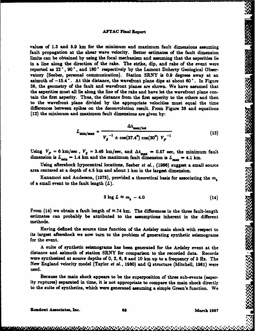
AFTAC lb.] Report

values of 1.3 and 5.9 km for the minimum and maximum fault dimensions assumingfault propagation at the shear wave velocity. Better estimates of the fault dimensionlimits can be obtained by using the focal mechanism and assuming that the asperities liein a line along the direction of the rake. The strike, dip, and rake of the event werereported as 22 ", 90 *, and 180" respectively by the Lamont Doherty Geological Obser-vatory (Seeber, personal communication). Station SRNY is 0.9 degrees away at anazimuth of -15.4 *. At this distance, the wavefront plane dips at about 60 ". In Figure38, the geometry of the fault and wavefront planes are shown. We have assumed thatthe asperities must all lie along the line of the rake and have let the wavefront plane con-tain the first asperity. Thus, the distance from the first asperity to the others and thento the wavefront plane divided by the appropriate velocities must equal the timedifferences between spikes on the deconvolution result. From Figure 38 and equations(12) the minimum and maximum fault dimensions are given by:

L adl/== = 1t ti(13)---vs-' * cos(37.4) cos(30) -13

Using Vp = 6 km/sec, Vs = 3.46 km/sec, and Atmw - 0.57 sec, the minimum faultdimension is Luda - 1.4 km and the maximum fault dimension is LIM - 4.1 km.

Using aftershock hypocentral locations, Seeber et a., (1988) suggest a small sourcearea centered at a depth of 4.5 km and a6 out 1 km in the largest dimension.

Kanamori and Anderson, (1975), provided a theoretical basis for associating the m,of a small event to the fault length (L).

3 log L P mb - 4.0 (14)

From (14) we obtain a fault length of $.74 km. The differences in the three fault-lengthestimates can probably be attributed to the assumptions inherent in the differentmethods.

Having defined the source time function of the Ardsley main shock with respect toits largest aftershock we now turn to the problem of generating synthetic seismogramsfor the event.

A suite of synthetic seismograms has been generated for the Ardsley event at thedistance and azimuth of station SRNY for comparison to the recorded data. Recordswere synthesized at source depths of 0, 2, 6, 8 and 10 km up to a frequency of 5 Hz. TheNew England velocity model (Taylor et aL., 1980) and Q structure (Mitchell, 1981) were .Iused. -

Because the main shock appears to be the superposition of three sub-events (asper-ity ruptures) separated in time, it is not appropriate to compare the main shock directlyto the suite of synthetics, which were generated assuming a simple Green's function. We

REondout Associates, Inc. 63 March 1987

APTAC ing Report

therefore compare the aftershock seismogram to the synthetics. To match the 5 Hz high 9frequency limit of the synthetics and eliminate microssismic noise, the data were bandprom filtered between .5 and 5 Hz prior to the comparison.

The vertical component traces are shown in Figure 39 with the appropriate datatrace placed at a depth of 4.5 km. The first three phases to arrive are thePg, PiP, and .PiP phases illustrated in Figure 40. Phases that are initially downgoing 0such as PiP arrive earlier as the source depth increases and phases that are initiallyupgoing, especially depth phases such as sPiP, arrive later as the source depth increases.The match of the synthetics to the first three arrivals of the data is quite good althoughthe amplitude are not well matched. In addition, approximately 3.5 ec after Pg thereis a clear phase on the data trace. Most likely it is ePmP, though this is not a prom- 0nent arrival in the synthetics and synthetic #PmP arrives slightly later for a sourcedepth of 4.s km.

Station RSNY at 44.548 * N 74.530 * W is 400 km from the epicenter of the Ardsleyevent and at nearly the same azimuth as station SRNY (-15.4' vs. -8.0' ). It recordedboth the main shock and the aftershock discumed above but at a much lower signal-to-noise ratio. Because the synthetic match at station SRNY was excellent and we have agood model for the far field displacement time history along this azimuth, we haveattempted to model the data at station RSNY.

A summary of the depth estimates for northeastern events is presented below inTable 5.

TABLE 5

Source Depths of Northeast U.S. Earthquakes

Date Event Maginitude Reported Depth This Study

Oct 07, 1983 Goodnow 5.2 mb 7,14 10

Jan 19, 1982 New Hampshire 4.5 mb 3-11 6Oct 11, 1963 Ontario 4.1 mU 12 14Oct 19, 1985 Ardsley 4.0 m 5 4.5Oct 02, 196 Quarry 2.3 me 0 0Aug 31, 192 Adirondack 2.6 m. ? 7Oct 23, 1964 Adirondack 3.4 me ? 12Oct 30, 19U Amsterdam 2.7 me 1May 29, 1983 Maine 4.2 mb 2 12

The suite of synthetics for RSNY were generated using a point source at depths of0, 2, 4, 6, 8, 10 and 12 km. The results were then convolved with an approximation tothe far field displacement time history so that a comparison could be made with the data(Figure 41). The vertical data recorded at RSNY in Figure 41 are placed at the depth

Remiout Associates, bie. .4 March I7

-D

d

z

InI

41

"4

CLif'SC381

EC

0 00

65

C1LCL.CLI

ra

0

66/

AS

I1;

*A*8 I.

*.60

lbsI

*~n A

U 0

"I

U ~

~1~

b.

E

-~ 0 04 J 'U - -a o0

67

APTAC Flu.] Report

determined from comparison of the synthetics and data at SRNY (4.5 kin). Althoughnoisy, the fit of the data to the synthetics is good. The depth phases are very wellmatched between seconds two and five as is the arrival at second nine. What has notbeen modeled is the high amplitude coda between these two sets of arrivals. This maybe the effect of scattering, multipathing, or the simplicity of the synthetic model.

Kuril/Kamchatka Data

The Kuril/Kamchatka data will be discussed collectively rather than event by eventas was done for the northeast U.S. data. The event and OSS-IV locations are shown inFigure 7. Sixteen events were studied, of which fourteen were assigned depths (Table 3). 0All of the events are above magnitude 4.5 and range in distance from 574 km to 1307 kmfrom OSS-V.

The OSS instrument was emplaced 380 m below the sea floor in 5467 m deep ocean.The primary motivations for placing the instrument in a borehole are to enhance thecoupling of the instrument and to remove the sensors from the noisy sea-bottom environ-ment. Soft sediments at the ocean bottom have strong shear-wave velocity gradients,which trap shear-wave energy close to the sea-floor interface. By installing the sensorswell below the sea floor, the shear wave noise is avoided. Unfortunately, being wellbelow the sea floor interface can complicate the receiver site effects. At typical compres-sional wave sediment velocities (2.0 km/sec) the travel time from the instrument to thesea-floor interface and back is 0.38 seconds. The two-way travel time for the sea-surfacereflection is 7.7 seconds. The sea-surfa&e reflection is the strongest of the two (Figure42-59). As seen from the data, the prominent sea-surface reflection would make anydepth phase arriving near 7.7 seconds difficult to identify. A pP phase arriving at 7.7seconds corresponds to an event depth of about 23 km.

For the northeastern U.S. data, adaptive polarization analysis was used to helpidentify phases. The apparent angle of incidence trace identified arrivals with similarphase velocities and the RZ trace helped identify true arrivals. The unusual location ofOSS-IV, beneath the sea floor, makes use of adaptive polarization analysis suspect. Astrong sea-bottom reflection adds downgoing arrivals to the usual upgoing waves. Theapparent angle of incidence trace would then become usele. and the RZ trace wouldindicate both P and SV type motion. Event KI (Figure 43 and 44) is an example of thistype of event. During the initial arrivals, the RZ trace is both positive and negative(usually a sign of Rayleigh type motion) and the apparent angle of incidence trace isconfused. In contrast, the sea-surface reflection, which does not include the sea-bottomreflections, has stable negative apparent angle of incidence and RZ trace.

Events with a large signal-to-noise ratio, K1, K3, K4, KS, K6, K7, K10, K11, andKIS all exhibit a common character in the first part of the wavetrain. The first arrival isgenerally small and is followed by three or more arrivals with increasingly large ampli-tudes in the next two seconds. The later arrivals could be either depth phases (pP, eP),source effects, or receiver site effects. The reported depths of the events eliminates depthphases as the source of these arrivals for all but the K7 event (6 km depth). If the

Rondout Assoclat", Inc. March 1987

AFTAC Final Report

arrivals are due to source effects then a remarkably consistent source mechanism wouldbe required for all of these events. Although source effects are certainly present in thedata, the regularity of the arrivals over so many events strongly suggests that they arecaused by site effects. The additional arrivals are also present in the sea-surfacereflection.

Uncertainty in the amount of skew correction, problems associated with the locationof the OSS and lack of good long range synthetics made depth determination for thisdata set extremely difficult. Four different seismologists with varying degrees of observa-tional experience independently evaluated the data for depth and obtained consistentpicks for only one of the 16 events (Table 6). Ironically, that event, KS, has no pub-lished depth. The depth determined by the observers for K5 was about 16 km.

TABLE 6

Differences in Travel Times Between the FirstArrival and the First Identifiable Depth Phase

as Picked by Four Analysts for the Kuril/Kamchatka Data

Eventi Analyst #I Analyst #2 Anlyst#3 Analyst #44.7 2.9 11.8 11.9

K3 3.5 3.6 5.0 7.4K4 3.2 5.4 14.0 10.0KS 5/5.5 .5.4 5.7 5.4KO 3.8 2.9 13.0 3.0K7 3.5 2.9 13.0 13.0K8 2.2 5.4 13.0 1.25

K10 3.2/5.3 4.6 2/3.9 10.7Kn 4.0 2.1/14.6 6.9 13.9K12 3.5 5.7 2.1/3 2.2K14 8.0 5.7 .8/9/16.2 4.1K15 5.5 4.6 4.8 3.9K16 4.8 4.6 9.5/10.6 11.3KIS 8.0 5.4 2.3/11 6.6K19 4.7 3.2 5.6 9.0K20 2.9 2.9 ? 5.2

Rondout Associates, Inc. 69 March 1987

41*

0 040 .

3

39.

3 .33

00

cv 04402 0A

V WCan

L414

71 ,

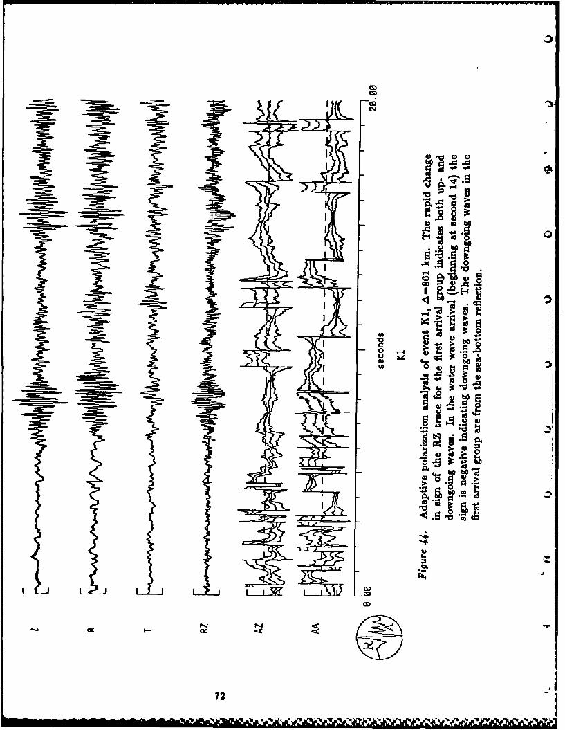
CID~9%

CY

I q~ mo

ba0

bo

I Ud"

(0 d .5 .

aa

-- 4

-~ I ~I~4.-bo N

.

cr..

72

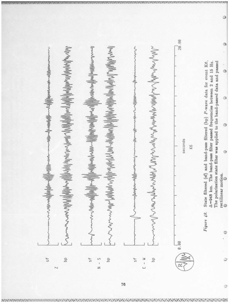
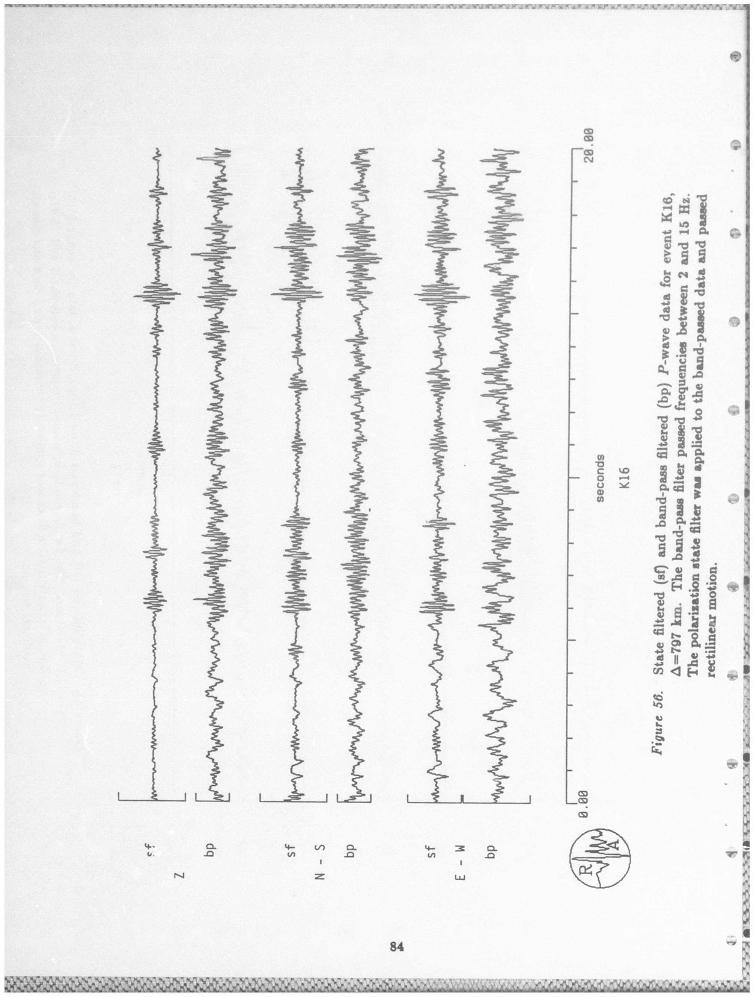
30

N

!iI114~.

i~ iii*

IiiJ~ji.o

L

9

00

0

I.- 0. (fl 0. 4.. ~In .0 en .o en

z LiJ

86

~ ~ - K

3a

14

r4U

.3 -

CDg

4- 39 CL4A 4A I

P14~ m La

87J

AFTAC lin Report

SECTION V.

SUMMARY AND CONCLUSIONS

Application of the depth phase method for event depth determination in the Snortheastr U.S. and the Kuril/Kamchatka are gave mixed results. In the northeast,excellent results were obtained (see Table 5) while in the Kuril/Kamchatka area verypoor performance was recorded. The conditions that led to the dramatic contrast in theresults can be used to quantify the method's strengths and weaknesses.

One major difference between the two data sets is signal-to-noise ratios. With the 0exception of the Amsterdam earthquake and quarry blast, all of the recorded signals forthe northeast events have good signal-to-noise ratios, whereas signal-to-noise ratios forthe Kamchatka data were poor. This was due, in part, to the difference in epicentral dis-tances; for northeast events all epicentral distances are less than 330 kin, while for theKamchatka data they ae all between 570 and 1301 kma. Also, the propagation paths 0from many of the Kamchatka events traverse a major tectonic boundary, the KurilTrench, and this may contribute to a decrease in signal-to-noise. The signal-to-noiseratio plays a significant role in the depth determinations. Tests of the polarization statefilter method used to help isolate depth phases have shown that performance degradessignificantly below signal-to-noise ratios of 1. This hampered the efforts to identifydepth phases for the Kamchatka events.

The second major difference between the data sets is the data quality. Data col-lected in the northeast U.S. were recorded by broad band stations RSNY and SRNY.Both record data digitally and have well known characteristics. The OSS data, collectedusing a remote sea-bottom recording system, has problems with skew, timing, and possi-bly instrument noise. The polarization methods described in this report require that thethree components of motion be accurately aligned in time. Although skew was correctedfor in the OSS data, some inaccuracies may have persisted.

The physical location of the recording stations also contributed to differencesbetween the data sets. Both RSNY and SRNY are well coupled stations at or near thefree surface of the Earth. In contrast, 0SS-IV is well below the sea floor in deep ocean.Superimposed upon the upgoing seimnic wavefleld at OSS-IV ae reflections from thesea-bottom interface and the sea surface. The resulting wavefteld is complicated, makinguse of the adaptive polarization method for phase identification of minimal value as wellas reducing the effectiveness of the polarization state filter.

Another difference that bears on the results is the way the two data sets were 0analysed. The northeastern o were compared to synthetic depth sections,wherea we simply attempted to pick upgoing and downgoing phases on the complexKamchatka seimogiams. The synthetic sismogrms guided our identification of phasesconsiderably and, without them, it would have been very difficult to identify properly-paired primary and depth phases in the northeastern data.

Readout Associates, Ile. 8 March 198T

APTAC Iml Report

The preceding discumion pointed out possible reasons that the depth phase methodgave depths consistent with reported depths for the northeastern U.S. data but did notwork on the Kamchatka/Kuril data. In the course of applying the method to thenortheastern data, we found that several other conditions were important for its success.The Ardsley event revealed that source complexity i possible in small events and thatthe phases associated with the complexity could be misidentified as depth phases. Sinceidentification of phases can be aided by synthetic seismogams, it is important to have ameasure of the validity of the models. A models' robustness could be tested by success-fully modeling the data from several different receiving stations. Unfortunately, we donot often have on-scale digital data, especially three-component data, from more thanone station in the northeast. Nevertheless, we can afford a certain degree of confidencein the modelling and interpretation of earthquakes we selected because: 1. the epicentersare well located by dense regional networks, 2. some of the depths are also well deter-mined by virtue of close-in permanent or temporary stations, 3. for more than half theearthquakes, fault-plane-eolutions have been obtained from P-wave first motions and 4.several regional velocity structures have been estimated from refraction experiments,teleseisnic residuals, and travel-time curves. More comparisons need to be made, how,ever, to establish whether the velocity models so derived (#4 above) are the mostappropriate for waveform modelling at the frequencies of interest. It is apparent fromthe comparisons we have presented here that the data are not perfectly modelled by thesynthetics. Future investigations should focus on improving theme results through betterunderstanding of both data and synthetics. Now that digital data are available fromregional networks , there in great potential for discovering much more about sourcemechanics and crusta phase propagation. Future insights can give us a better idea ofhow to model the entire source-path-receiver system.

In conclusion, the depth phase method for depth determination can work quite wellunder certain conditions. The problem that remains to be solved is to identify whenthese conditions are met for a particular data set.

Readout Associates, Inc. s9 March 1987

REFERENCES

ArcambanC. B., J. C. Bradord, P. W. Broome, W. C. Dean, E. A. Finn, and R. L.Sax, "Data processing techniques for the detection and interpretation of teleseismicigals," Proc. IEEvol. 53, pp. 1860-1884, 1965.

Bakun, W. H., R. M. Stewart, and C. G. Bufe, "Directivity in the highi-frequencyradiation of small eathquake1," Bull Seism. Soe. Am., vol. 68, pp. 1253-1263, 1978.

Barstow, N. L., J. A Carter, and A. Suteau-Henson, "Focal depths of shallow localearthquakes from comparison of polarization filtered data with synthetics," abatr.Earthquake Not"., vol. 57, No.1, pp. 1800.188, 1986.

Brown, E. J. and J. Z. Ebel, "An investigation of the January 1962 aftershock sequencenear Laconia, New Hampshire," submitted to BErth quake Note", 1985.

Douglas, A., J. A. Hudson, and P. D. M&%Wal, "Earthquake seismograms that showDoppler effects due to crack propagation," Geophy.. J., vol. 64, pp. 163-185, 1981.

Ebel, J. E. and J. P. McCaffrey, S. J., "Hypocmntral parameters and focal mechanism ofthe 198 earthquake near DIIxfisld, Maine," Earthquake Note., vol. 55, No. 2, pp.21-24, 1984.

Frankel, A. and H. Kanamri, "Determination of rupture duration and stress drop forearthquakes in southern Califoria" Bull. Scism. Soc. Am., vol. 73A, pp. 1527-1552, 1983.

Hatell, S. H., "Earthquake aftershocks as Green's functions," Geophys. Res. Letters,vol. 5, pp. 1-4, 1978.

Harvey, D., "Seismogram synthetics using normal mode superposition: the locked modeapproximation method," GeophVe. J. Roy. Aetr. Soc., vol. 66, pp. 37-69, 1981.

Houlday, M., Rt. Quittmeyer, K. Mrotek, and C. T. Statton, "Recent seismicity in northand east-central New York State," Earthquake Notes, vol. 55, No. 2, pp. 16-24,1984.

Kanamori, H. and D. L. Anderson, "Theoretical basis of somae empirical relations inseimology," Bvul Scisin. See. Am., vol. 65, pp. 1073-1095, 1975.

Kanamori, H. and G. S. Stewart, "Seismological aspects of the Guatemala earthquake ofFebruary 9, 1976," J. GeephV.. Re., vol. 83, pp. 3427-3434, 1978.

Kanamori, Hf., "A semi-empirical approach to prediction oflong-period ground motionsfrom great earthquakes," Bull. Seism. Soc. Am., vol. 69, pp. 1654-1670, 1979.

Khattri, K., "Body wave directivity functions for two-dimensional fault model andkinematic parameters of deep focus earthquake," J. Geophye. Res, vol. 77, pp.2062-2071, 1978.

Mitchell, B. J., "Regional variation and frequency dependence on Q 0in the crust of theUnited State.," BSSA, vol. 71, No. 5, pp. 1531-1538, 1981.

90r

Mueller, C. S., "Source pulse eaceetby deconvolutlon of an empirical Green'sfuanction," G..pkp. Res. Lettes, vol. 12, pp. 33-36, 1965.

Pulli, J. J., J. C. Nabelek, and J. M. Sauber, "Source parameters of the January 19, 1962Gaza, New Hampehire earthquake," absr. Ekrthquake Not"s, vol. 54, No. 3, pp. 28-29, 1963.

Samson, J. C., "Matrix and Stokes vector representations of detector, for polarizedwaveform: theory with some applications to teleseismic waves," Geophys. J. Roy.Astr. Soe., vol. 51, pp. 583-603 1977.

Samson, J. C. and J. V. Olson, "Data-adaptive polarization filter, for multichannelgeophysical data," Geophsics, vol. 46 No. 10, pp. 1423-1431, 1961.

SchleshnMIller, E., N. L. Barstow, and A. L. Kafka, "The July 1961 earthquakesequence near Cornwall, Ontario and Massena, New York," Earthquake Not"s, vol.54, No.3, pp. 11-26, 1963.

Seeber, L., E. Cramawick, N. Barstow, J. Armbruster, G. Suares, K. Colea, and C. Aviles,"Grenville structure and the Central Adirondack seismic None including the October7, 1963 mainshock-aftershock sequence Canadian Geophysical Union Meeting,"Halfax, Nov Scotia, 1964.

Seeber, L., E. Craaswick, J. Armbruster, and N. Barstow, "The October 1963 Goodnow,NY aftershock sequence; regional sneismilcity and structural features in theAdirondacks," ACU abet., vol. 65, No.16, p. 239, 1964b.

Seeber, L., J. G. Armbruster, and D). Coyle, "A prolonged, but spatially concentratedearthquake sequence at the northern outskirts of New York City," abstr. SSA,Earthquake Not"s, vol. 57, No. 1, p. 16, 1966.

Suarez, G., L. Seeber, C. Avilas, and Z. Schlesinger, "The Goodnow, NY earthquake:results of a broad band teleseismic analysis," AGU abstr., vol. 65, No.16, p. 239,1984.

Sutton, G. H. and P. W. Pomeroy, "Analog analysis of seismograms recorded onmagnetic tape," J. Geophys. Rss., vol. 66, pp. 2791-2615, 1963.

Taylor, S. R., M. N. Tokac., and M. P. Chaplin, "Crustal structure of the NortheasternUnited States: Contrasts between Grenvill and Appalachian Provinces," Science,vol. 206, pp. 595-597, 1960.

Taylor, S. R. and B. J. Qualheim, "Regional seismic test network site descriptions,"UCID-19709, Lawrence Livermore Laboratory, 1963.

Trifunac, M. D. and 3. N. Brune, "Complexity of energy release during the ImperialValley, California, earthquake of 1940," Bull Scism. Soc. Am., vol. 60, pp. 137-160,1970.

Wahlstrom, R., "The North Cower, Ontario, earthquake of 11 October 1983; focalmechaism and aftershocks," submitted to Earthquake Notes, 1965.

91

Whites J. Z., "Motion product Nmpm," Ge.php., vol. 29, pp. 2M8298, 1964.Yang, J. and Y. P. Aggaiwal, "Selumoteetnc of northeaatern United State. and

adjacuat Cmanaa, J. of Geoph.. R"., vol. 86, No.B6, pp. 4981-4998, 1961.

00

92

DI3TRXDUTZO LIST

FOR UNCLASSIr RPOSTSDARPA-UNDED PROJECTS

(Last Reviseds 11 NIay 87)

lUCIt !T NUMUR OF COPIRS

D3PARTGIUT or DEWEMI

DARPA/QBnATTL: Dr. i. Alevdne and Dr. R. Blandford 21400 Wilson BoulevardArlington, VA 22209-2308

DAPA/M1400 Wilson BoulevardArlington, VA 22209-2308

Defense Intelligence Agency IDirectorate for Scientific and

Technical inteliigenceWashington, D.C. 20301

Defense iMclear AgencyShook PhysicsWashington, D.C. 20305-1000

Defense Technical Informtion Center 12Cmeron StationAlexandria, VX 22314

DELPARtMNT Or TIM AIR FORCI

AP=G/LWE 2ATTM. Dr. J. Cipar and Mr. J7. LevkowiczTerrestrial Sciences DivisionEanscom APB, MA 01731-5000

APOSR/ma IATTN. DirectorBldg 410, Room C222Bolling AS, Washington, D.C. 20332

APTAC/CAATTN. STIPNO OfficerPatrick APB, PL 32925-6001

APTAC/TQ 3Patrick APB, PL 32925-6001

AI WLNT ISGKirtland APB, NN 07171-6008

8

DEPARTWENT OF THE XAVY

ATUs Dr. J. A. BallardCode 543NSTL Station, NO 39529

DEPAM OF ENERGY 0

Department of ergy ATTNz Mr. Nax A. Koontx (DP-52)International Security Affairs1000 Independence AvenueWashington, D.C. 20545 0

Lavrence Livermore National Laboratory 2ATTN, Dr. J. Hannon and Dr. N. NordykeUniversity of CaliforniaP.O. Box 08Livermore, CA 94550

Los Alamos Scientific Laboratory 2ATTt Dr. K. Olsen and Dr. T. WeaverP.O. Box 1663Los Alamos, 34 87544

Sandia Laboratories 1ATTU& Mr. P. StokesGeosciences Department 1255Albuquerque, H 87185

OTMM GOVZRNM1= AGENCIES3

Central Intelligence AgencyATTNs Dr. L. TurnbullOS/NED, Room 5G48Washington, D.C. 20505

U. S. Arms Control and Disarmament Agency -ATTK; Dr. M. EimerVerification and Intelligence Bureau, Rm 4953Washington, D.C. 20451

U. S. Arms Control and Disarmament Agency IATTs Mrs. H. BoinkesMultilateral Affairs Bureau, Rm 5499Washington, D.C. 20451

U. S. Geological Survey 1ATTEs Dr. T. RanksNational Earthquake Research Center345 Middlefield RoadHenlo Park, CA 94025

94

OHRGOVE===ET AGENIES (continued)

9. S. Geological Survey NS-913AM&~ Dr. Rt. MasseGlobal seismology Branchamx 25046, Stop 967Denver Federal CenterDenvr CO 80225

UNIVERSITIES

Boston CollegeATTI: Dr. A. KafkaWestern Observatory361 Concord RoadWestan, MA 02193

California institute of TechnologykTU: Dr. D. larkriderSeismological LaboratoryPasadena, CA 91125

Columbia UniversityATI Dr. L. SykesLaont-Daherty Geological ObservatoryPalisades, my 10964

Cornell UniversityATTR: Dr. M. BarazangiISTOC

Snee HallIthaca, MY 14853

Harvard UniversityATTNs Dr. J7. WoodhouseHoffman Laboratory20 Oxford StreetCAmbidge, Ma 02136

Massachusetts Institute of Technology 3ATTN. Dr. S. Solcoan, Dr. N. Toksoz, and Dr. T. JordanDepartment Of Earth and Planetary SciencesCambridge, N& 02139

Southern Methodist UniversityIATTN. Dr. E. HerrinGeophysical LaboratoryDallas, TZ 75275

State University of New York at BinghamtonIATTN$ Dr. V. WuDe partmlent of Geological SciencesVestal, NY 13901

95

UNIVERSITIES (continued) A

St. Louis University 2ATTE: Dr. 0. mattli and Dr. R. HerruannDepartment of Barth and Atmospheric Sciences3507 LacledeSt. Louis, NO 63156

The Pennsylvania State University 1ATTNt Dr. S. AlexanderGeoscience. Department403 Deike BuildinqUniversity Park, Ph 16802

University of Arizona 1ATTI: Dr. T. WallaceDepartment of GeosciencesTucson, AZ 85721

University of California, Berkeley 1ATTNs Dr. T. IHc~villyDe par tment of Geology and GeophysicsBerkeley, CA 94720

University of California Los Angeles 1ATTNh: Dr. L. Knopoff405 Bilgard AvenueLos Angeles, CA 90024

University of California, San Diego 1ATTN: Dr. J. OrCuttScripps Institute of OceanographyLa Jolla, CA 92093

University of Colorado1ATTNt Dr. C. ArchanbeauClUEBoulder, CO 80309

University of Illinois1ATTN: Dr. S. GrandDepartment of Geology1301 Went Green StreetUrbana, IL 61801

University of Michigan1IATTU: Dr. T. LayDepartment of Geological SciencesAmn Arbor, MI 48109-1063

University of Nevada1IATTNt Dr. K. Priestley

Mackay School of MinesReno, NV 89557

96

FUNIVERSITIES (continued)

University of Southern CaliforniaATTNs Dr. K. AkiCenter for Earth SciencesUniversity ParkLos Angeles, CA 90089-0741

DEPARTMENT OF DEFENSE CONTRACTORS

Applied Theory, Inc.ATTN: Dr. J. Trulio930 South La Brea AvenueSuite 2Los Angeles, CA 90036

Center for Seismic Studies 2ATTN: Dr. C. Romney and Mr. R. Perez1300 N. 17th Street, Suite 1450Arlington, VA 22209

ENSCO, Inc.ATT'Ns Mr. G. Young5400 Port Royal RoadSpringfield, VA 22151

ENSCO, Inc.ATTN: Dr. R. Kamerait445 Pineda CourtMelbourne, FL 32940

Gould Inc.ATTNt Mr. R. J. WoodardChesapeake Instrument Division6711 Baymeado DriveGlen Burnie, MD 21061

Pacific Sierra Research Corp. IATTNt Mr. F. Thomas12340 Santa Monica BoulevardLos Angeles, CA 90025

Rockwell InternationalATTN: B. Tittmann -'

1049 Camino Dos RiosThousand Oaks, CA 91360

Rondout Associates, Inc.ATTN: Dr. P. PomeroyP.O. Box 224Stone Ridge, NY 12484

Science Applications, Inc. 1ATT'Ns Dr. T. Bache, Jr.P.O. Box 2351La Jolla, CA 92038

DEPARTMENT OF DEFENSE CONTRACTORS (continued)

Science Horizons 2ATTN: Dr. T. Cherry and Dr. J. Minster710 Encinitas Blvd.Suite 101Encinitas, CA 92024

Sierra Geophysics, Inc. 2ATTNs Dr. R. Hart and Dr. G. Mellman11255 Kirkland WayKirkland, VA 98124

SRI InternationalATTNs Dr. A. Florence333 Ravensvorth AvenueMenlo Park, CA 94025

S-Cubed A Division ofMaxwell Laboratories Inc.ATTN: Dr. S. DayP.O. Box 1620La Jolla, CA 92038-1620

S-Cubed, A Division ofMaxwell Laboratories Inc.ATTNs Mr. J. Murphy11800 Sunrise Valley DriveSuite 1112Reston, VA 22091

Teledyne Geotech 2ATTN: Dr. Z. Der and Mr. W. Rivers314 Montgomery StreetAlexandria, VA 22314-1581

Woodward-Clyde Consultants 2ATTNt Dr. L. Burdick and Dr. J. Barker556 21 Dorado StreetPasadena, CA 91109

NON-US RECIPIENTS

Blacknest Seismological CenterATTNs Mr. Peter MarshallAtomic Weapons Research EstablishmentUK Ministry of DefenseBrimpton, Reading RG7-4RSUnited Kingdom

National Defense Research InstituteATTN: Dr. Ola DahlmanStockholm 80, Sweden

96

IMON-0U SC IPIUTS

ATTN. Dr. trode RingdalP.O. amx 313-2007 1jsherNorway

OTHER DISTRIBUTION

To be determined by the project office

99.