unclassi fied a d 260955 v - vibrationdata · unclassi fied 260955 a dv ... the effects of rocket...

UNCLASSI FIED

260955VA D

DEFENSE DOCUMENTATION CENTERFOR

SCIENTIFIC AND TECHNICAL INFORMATION

CAMERON STATION. ALEXANDRIA. VIRGINIA

UNCLASSIFIED

NOTICE: When government or other drwaings, speci-fications or other data are used for any purposeother than in connection with a dsefinitely relatedgovermenmt procurement operation, the U. S.Government thereby incurs uo xesponsibility, nor anyobligation whatsoever; an. the fact that the Govern-ment may have formlated, ftw'ished, or in any waysupplied the said dravinfs, specifications, or otherdata is not to be regarded by implication or other-wise as in any manner licensing the bolder or anyother person or corporation, or conveying any rightsor permission to manufecture, use or sell anypatented invention that may in any way be relatedthereto.

WADC TECHNICAL REPORT 58-343

VOLUME I!

METHODS OF SPACE VEHICLE NOISE PREDICTION

" 6 Peter A. Franken

and

The Staff of Bolt Berenek and Newman Inc.

0

x ×SEPTEMBER 1960

I G AIR . . ...... DIVISIO N

WRIGHT AIR DEVELOPMENT DIVISION

NOTICES

When Government drawings, specifications, or other data are used for any purpose otherthan in connection with a definitely related Government procurement operation, the United StatesGovernment thereby incurs no responsibility nor any obligation whatsoever; and the fact thatthe Government may have formulated, furnished, or in any way supplied the said drawings,specifications, or other data, is not to be regarded by implication or otherwise as in any mannerlicensing the holder or any other person or corporation, or conveying any rights or permissionto manufacture, use, or sell any patented invention that may in any way be related thereto.

Qualified requesters may obtain copies of this report from the Armed Services TechnicalInformation Agency, (ASTIA), Arlington Hall Station, Arlington 12, Virginia.

This report has been released to the Office of Technical Services, U. S. Department of Com-merce, Washington 25, D. C., for sale to the general public.

Copies of WADD Technical Reports and Technical Notes should not be returned to the WrightAir Development Division unless return is required by security considerations, contractual obliga-tions, or notice on a specific document.

WADC TECHNICAL REPORT 58-343

VOLUME II

METHODS OF SPACE VEHICLE NOISE PREDICTION

Peter A. Franken

and

The Staff of Bolt Beranek and Newman Inc.

SEPTEMBER 1960

Flight Dynamics Laboratory

Contract No. AF33(616)-6217

Project No. 1370

Task No. 13786

WRIGHT AIR DEVELOPMENT DIVISION

AIR RESEARCH AND DEVELOPMENT COMMAND

UNITED STATES AIR FORCE

WRIGHT-PATTERSON AIR FORCE BASE, OHIO

300 - May 1961 - 28-1042

FOREWORD

This report was prepared for the Flight DynamicsLaboratory, Wright Air Development Division, Wright-PattersonAir Force Base, Ohio. The research and development work wasaccomplished by Bolt Beranek and Newman Inc., Cambridge,Massachusetts, and Los Angeles, California, under Air ForceContract No. AF33(616)-6217, Project No. 1370, "DynamicProblems in Flight Vehicles," Task No. 13786, "Methods ofNoise Prediction Control and Measurement." Mr. D. L. Smithof the Dynamics Branch, Flight Dynamics Laboratory,Aeromechanics Division, Directorate of Advanced SystemsTechnology, is Task Engineer. This report is denotedVolume II, following WADC TR 58-343, "Methods of FlightVehicle Noise Prediction." This report is intended as acritical summary of practical information now available,and an investigation of problems not reported in the existingliterature. It is anticipated that this report will berevised as never methods and procedures are developed. Thework which iab _nitiated in May 1957 will, therefore, continue.

Major contributions to this report were made byDrs. I. Dyer, M. A. Heckl, E. M. Kerwin, Jr., and E. E. Ungar,of Bolt Beranek and Newman Inc. This assistance is gratefullyacknowledged.

WADC TR 58-343Volume II

ABSTRACT

Possible sources of noise in space vehicles arereviewed. Information is summarized, describing the variousfluctuating pressure fields that may exist at the vehicleexterior. The response of the vehicle structure to thesepressure fields and the resulting radiation of noise to theinternal spaces are studied analytically. The need for newtheoretical and experimental knowledge in specific areas isemphasized.

The effects of rocket engine noise on communicationand hearing are considered in detail. General comments aremade concerning vehicle and equipment design for noise control.

PUBLICATI ON REVIEW

This report has been reviewed and is approved.

FOR THE COMMANDER:

AJOHN P. TAYLOR

Colonel, USAFChief, Flight Dynamics Laboratory

iiiWADC TR 58-343Volume II

TABLE OF CONTENTS

Section Page

INTRODUCTION TO VOLUME II .. .......... . 182

VI. NOISE SOURCES ..... ............... . 186

A. Rocket Engine Noise .......... 186

1. Test Stand Operation . ....... . 186

2. Effects of Forward Motion ...... .. 190

3. In-Silo Operation .. .......... . 191

4. Correlation Properties of Rocket

Noise ..... ................ . 193

APPENDIX TO VI A -- EFFECTS OF MOTION ON

WAVE PROPAGATION .... .............. 195

B. Pressure Fluctations in a Turbulent

Boundary Layer ....... . ........ 198

1. Spectrum Shape and Characteristic

Dimensions for Subsonic Boundary

Layers .... ............... . 198

2. Roughness-Induced Noise ........ . 200

3. Supersonic Boundary Layers ..... 202

4. Summary .... ............... . 203

C. Wake Noise . . . . ............. 204

D. Base Pressure Fluctuations ....... . 207

E. Oscillating and Moving Shocks ..... 210

F. Flow Over Cavities ... ........... 214

G. Flight Through a Turbulent Atmosphere . . 216

1. Subsonic Flight Speeds ... ....... 216

2. Supersonic Flight Speeds ...... 218

3. Retro-rocket Turbulence ........ . 220

H. Pressure Due to Micro-Meteorite Impacts 221

I. Discussion .... ............... 223

WADC TR 58-343 ivVolume II

TABLE OF CONTENTS

Section Page

VII. STRUCTURAL RESPONSE ..... .......... ... 225A. Response of Plates to Moving Shocks . . 226

1. Shock Moving at Constant Velocity . 228

2. Sinusoidally Oscillating Shock . . . 232

B. Response of Plates to Temporally Random

Pressure Fields: Atmospheric Turbulence,

Rocket Noise .... .............. . 234

1. Response to Atmospheric Turbulence 234

2. Response to Sound ........... .. 237

a. Response of Resonant Structures

to Sound ... ............ . 237

b. Sound Transmission Through

Finite Cylinders . ....... .. 238

C. Response of Plates to Pressures That Are

Random in Space and Time . ........ .. 241

1. General Solution .. .......... . 242

2. Response to Boundary Layer Pressure

Fluctuations ... ............ . 243

a. Response at Coincidence ..... .. 245

b. Response Below and Above

Coincidence . . . . ......... 247

3. Response to Micro-Meteorites . . . 248

VIII. NOISE IN INTERNAL SPACES ... .......... .. 255

A. Structural Radiation and Acoustic

Damping ...... ................ ... 256

1. "Equivalent" Transmission Loss 258

2. Sound Radiation and Structural

Damping .... ............... ... 259

B. Ventilation Noise Within Space Vehicles . 261

WADC TR 58-343 vVolume II

TABLE OF CONTENTS

Section Page

IX. THE EFFECTS OF NOISE ON MAN: NUMERICAL

EXAMtLE ...... ................... . 267

A. Example -- Space Vehicle Noise Levels . . 268

B. Effects of Noise on Cummunication . ... 272

1. Intelligibility of Received Speech

During Launch ... ........... . 273

2. Intelligibility of Transmitted

Speech During Launch . ........ 275

3. Temporary Threshold Shift Following

Subsonic Boost .. ........... . 276

C. Hearing Damage Risk .... ............ 276

X. DESIGN CONSIDERATIONS ... ............ 279

REFERENCES FOR VOLUME II .. .......... . 285

ERRATA IN VOLUME I ... ............. 291

ILLUSTRATIONS - FIGURE 75 THROUGH 118 293

WADC TR 58-343Volume II vi

TIST OF FIGURES

Figure Title

75 Source Location as a Function of Strouhal Number76 Geometry for Rocket-Deflector Configuration

77 Correction for Changes in Ambient Temperatureand Pressure

78 Reference Free Field Sound Pressure Level atMissile

79 Sound Pressure Level Change as a Function ofMach Number

80 Change in Sound Pressure Level of Large Rockets

81 Differences Between Highest Noise Levels inUnlined I-Tube Silo and Above Ground

82 Differences Between Highest Noise Levels in LaunchDuct of Unlined Double-U Silo and Above Ground

83 Angular Correlation Around Missile

8 .Effects of Forward Motion: source and ReceiverGeometry

85 Effects of Forward Motion: Changes in Angle andObserved Wavelength

86 Effect of Forward Motion on Near-Field SoundPressure Level Contours of Contemporary TurbojetEngine

87 Boundary Layer Turbulence Spectra

88 Velocity Fluctuations in Supersonic BoundaryLayers

89 Qualitative Comparison of Noise Radiation from aJet and from a Wake

90 Measured Acoustic Power of F-100 Aircraft inFlight (Reference 6.13)

WADC TR 58-343Volume II

Vi

LIST OF FIGURES

Figure Title

91 Sketch of Flow in a Supersonic Wake

92 Typical Static Pressure Distribution over aSupersonic Vehicle

93 Frequency of Shock Oscillations on SpikedBodies (Reference 6.23)

94 Frequency of Sound Radiated in Cavity Flow

(Reference 6.26)

95 Plate Subject to Discontinuous Pressure

96 Steady and Varying Pressure Distributions

97 Proposed Shape of Random or Grazing IncidenceTransmission Loss of Cylinder (Broad-Band NoiseExcitation)

98 Characteristic Transmission Loss and RadialResonance Frequency of Cylindrical Steel orAluminum Shells

99 Radiation Factor for Travelling Waves on anInfinite Plate

100 Radiation Factor for Travelling Waves on aFinite Plate

101 Effect of Fluid Flow on Radiation Factor forStanding Waves on an Infinite Plate

102 Fan Noise Spectra

103 End Reflection Loss at the Open End of SquareDucts

104 Grille Noise for Core Area of 1 Square Foot

105 Relative Sound Pressure Level in a Room

106 "Free Space" Rocket Noise Levels at Launch

WADC TR 58-343Volume II viii

LIST OF FIGURES

Figure Title

107 Detail of Double Wall Construction in Example

108 Double Wall Resonance Frequency

109 TL for Panels near and Above the CoincidenceFr 8quency, fc

110 Approximate Transmission-Loss Increase (ATL) Dueto Acoustical Blankets

ll C2 , Correction to TL for Maximum Effect of

Standing Waves in Medium-Sized Receiving Space

112 C3 , Correction to TL for Reverberation in Large

Receiving Spaces

113 Noise Reduction of Double Wall in Example (SeeFigure 107 for Wall Detail)

114 IntellIg-lb1ity of Received Speech During Boost

115 Intelligibility as a Function of Articulation Index

116 Noise Attenuation of Present-Day High-AltitudeHelmet, Headset Cushion and Differential Microphone

117 Intelligibility of Transmitted Speech During Boost

118 Hearing Damage Risk During Boost

WADC TR 58-343Volume II ix

INTRODUCTION TO VOLUME II

The present report is denoted Volume II, following WADC

TR 58-343, "Methods of Flight Vehicle Noise Prediction." The

numbering system of pages, figures, equations, and sections

started in TR 58-343 is continued in this report. Although

this procedure may be somewhat unconvenuional, it serves to

emphasize to the reader the interdependence of the material

in the two volumes and should avoid possible confusion

arising from duplication of numbers.

This report is not intended to be either a collection of

engineering formulas or an exhaustive detailed report of

results available in the literature. Rather, the report is

intended as a critical summary of practical information now

available, and an investigation of problems not reported in

the existing liter'ature. An important feature of this report

is the assembly of general analytical formalisms useful in

studying the response of structures to various forcing fields,

and the reradiation of noise by the excited structures.

The general procedure for determining noise in space

vehicles may be summarized as follows:

1. Describe the forcing field.

2. Calculate the structural response.

3. Determine the internal noise.

Review of the incomplete information now available

indicates that four potential sources of noise in space

vehicles appear predominant:

1. Rocket engine noise

2. Flow noise (turbulence in boundary layers,wakes, and cavity flow)

WADC TR 58-343VolUme II -182-

3. Separation and staging transients

4. Mechanical equipment

Under certain circumstances, moving shocks and wakenoise may become significant sources, but no definite experi-

mental evidence of the importance of these sources exists.

Table A is an index to the source and response informa-

tion contained in this report:

TABLE A

Source ResponseData Calculation

Rocket Engine VI A III (Plates)

Noise VII B 2 (Cylinders)

Boundary Layer VI B VII C 2Turbulence

Base VI D VII C 3Primary TurbulenceSources Cavity Flow VI F VII C 3 (Turbu-

Fluctuations lence)

Staging VI A (siloTransients ignition)Mechanical II C VII A,Equipment VIII BMoving Shocks VI E VII A

Wake VI C III (PlatesNoise VII B 2 (Cylin-

ders)Atmospheric VI G VII B 1Turbulence

Micro-meteorites VI H VII C 3

In addition to the sources listed in Table A, engine vibra-

tions and unsteady thermal stresses could under some

circumstances become noise sources. These subjects have not

been studied in this report.

WADC TR 58-343Volume II -183-

Study of this source and response information shows

that at present theory is often idealized and that experi-

mental results are often incomplete. Many important

questions remain to be answered, and definitive prediction

procedures cannot be formulated. It is important that these

uncertainties be emphasized, so that predictions based on

current information are interpreted properly.

In order to determine the internal noise, two steps are

required. First, the mean square velocity of the surface

bounding thc region of interest i- converted into a mean

square pressure radiated into a perfectly absorbing space.

This step is described in Part A of Section VIII. Then the

mean square internal pressure is adjusted to account for

geometry and absorption, as described in Section IV.

Certain-mater4 1 in Volume I (Sections I - V) has been

replaced by more current and complete information in the

present volume. Table B lists these replacements.

TABLE B

Part of Part of Volume IIVolume I Containing

Subject Replaced Replacement

Rocket engine noise II A 4 VI A

Effects of forward II A Vi A (Appendix)motion on Jet noise

Boundary layer noise II B 1 V! B

Atmospheric turbulence II B 2 VI G

A list of minor errata in Volume I is given at the end of

the present volume. Errata are not listed for those parts of

Volume I that are being replaced.

WADC TR 58-343Volume il -184-

References are numbered serially within each Section

and are listed following Section X.

WADC TR 58-3413Volume 11 -185-

SECTION VI

NOISE SOURCES

A. Rocket Engine Noise

Section II presented a procedure for estimating rocket

engine noise along a vehicle surface. On the basis of new

and improved information that has become available since the

preparation of Section II, these procedures have been revised

and up-dated. In addition to test stand and in-flight opera-

tion, the material has been extended to cover in-silo

operation. Some comments on the correlation of noise at

different positions on a vehicle surface are also included.

1. Test Stand Operation

The sound pressure level* in octave bands over the sur-

face of a rocket-powered vehicle during static firing on a

test stand is given by:

1 2SPL =lO log 9 mv + SPLo - 20 log R - AB (87)

where 1/2 my2 is the mechanical stream power of the rocket

exhaust in watts, SPL0 is the reference sound pressure level

in an octave band, for R equal to 1 foot, R is the distance

from the point in question on the vehicle surface to the noise

source location in the Jet stream, and AB is the correction

for ambient conditions.

The various steps in the procedure to determine SPL in

octave bands from the above equation are summarized as follows:

* Sound pressure level is defined as

SPL = 20 log1 o Po db

where p is the rms sound pressure in microbars, and p isthe reference sound pressure of 0.0002 microbar.


1. Compute the mechanical stream power of the

rocket, which is given by 1/2 mv 2 in watts,

where m is the mass flow of the rocket and

v is the expanded jet velocity, the ratio

of thrust to mass flow. In MKS units, m is

in kilograms/second and v is in meters/

second.

2. Find the average source distance xo, which

is the distance from the rocket nozzle to

the average location of the noise source of

frequency f. For a rocket nozzle of diameter

D, the average source distance in terms of

xID is given as a function of Strouhal

number f by the lower curve in Figure 75.

This curve applies for a vehicle mounted

vertically firing into a bucket deflector

that is open at the two ends only and located

approximately 15 feet below the rocket nozzle.

Data are also available for a vehicle-deflector

config'ration where the deflector was located

approximately 40 feet from the rocket nozzle

and was an open curved scoop. Except for the

higher values of Strouhal number, it is seen

that the source distance x for this latter0configuration is 3 to 5 times greater. Indi-

cations are that the nozzle-deflector distance

a may appreciably influence the noise genera-

tion in the jet stream, and consequently

affect the location of the noise sources. We

suggest the use of the lower curve in Figure

75, since it will give results that are conser-

vative for most practical vehicle-deflector

configurations.


3. Compute the source-to-receiver distance R

appropriate to the geometry (see Figure 76).

For cases in which-the exhaust stream extends

directly back of the vehicle along the longi-

tudinal axis of the vehicle, or where x is

less than a:

R = x + x0 (88)

where x is the distance from the rocket exhaust

nozzle plane to the observation point, and x0

has been obtained in Step 2 above.

When x0 is greater than a, i.e., downstream

from the deflector, R is given as follows:

R = [(x + a)2 + (x0 - a) 2 ] (89)

4. Determine the correction for ambient tempera-

ture and pressure changes, AB, from Figure 77.

(This is Figure 32 of Volume I, repeated here

for convenience.) AB = 0 db for the reference

conditions of 5200 R and 14.7 pounds/sq. in.

5. Determine the reference free field sound

pressure level, SPL0 , in octave bands from

Figure 78. SPL is given as a function of the0 fD

Strouhal number, v

6. Combine the results of Steps 1 through 5 in

Equation (87) to obtain the sound pressure

level in octave bands that would exist at the

point in question in the absence of a rigid

surface. If the levels actually existing at

the external surface of the vehicle are


desired, these levels should be increased by

approximately 6 db in the frequency range

given by:

fD > Ca D (90)v - rVDveh

where c a is the ambient speed of sound and

Dveh is the vehicle diameter. At lower

frequencies, there is no pressure doubling

effect, and hence no correction to be applied.

Several workers have suggested on physical grounds that

the velocity appearing in the Strouhal number (see Steps 2

and 5) should be ca rather than v. At present, this choice

cannot be clearly resolved.

It was suggested in Section II that the broadness of the

rocket noise spectrum may be due to the presence of multiple

nozzle configurations usually found in large vehicles.

However, noise spectra from single-engine (4 ft in diameter)

firings are just as broad as data from a rocket with two

nozzles, each about 4 ft in diameter, spaced 10 ft on centers.

These results suggest that rocket noise may be inherently

broader in spectrum shape than turbojet noise, although more

comparative data on single- and multiple-nozzle operations

should be gathered to clarify this situation. However, in

the above procedure, use D as the diameter of a single

nozzle even for multiple-nozzle operation. In calculating

the mechanical stream power, use the total mass flow of all

of the engines in simultaneous operation.

Little quantitative information is now available on the

effects of water spray at the exhaust deflector. Qualita-

tively, water spray has been found to reduce the noise levels


only when the water mass flow is greater than the exhaust

gas mass flow.

2. Effects of Forward Motion

Following vehicle lift-off, the noise levels over the

surface of the vehicle can be affected in several ways.

These effects of forward motion include changes in wave

propagation, operating conditions, wave number k, noise

radiation (hemispherical to spherical), and angle between

the Jet stream and the vehicle axis.

The effects of motion on the wave propagation in the

medium between the source and the receiver have been taken

into account in a simple way, as described by Powell ° '- - V.

The sound pressure level at the vehicle surface is reduced

by forward motion at a subsonic Mach number M. The amount

of this reduction is given by the quantity ASPLm, which is

approximately:

zSPL = 20 log (l - M) (91)

At supersonic speeds, no rocket noise can propagate to the

space vehicle surface. A plot of ASPL as a function ofmM is given in Figure 79.*

Changes in rocket engine operating conditions, such as

mass flow and rocket exhaust velocity, occur during flight

and affect the amount of noise produced. For given values

of mass flow m and exhaust gas velocity v relative to the

values for the vehicle at rest, m0 and v0 , the change in

.The effects of motion on wave propagation are discussedin more detail in the Appendix to this Section.


sound pressure level, ASPL, can be determined directly

from Figure 80.

As the vehicle moves away from the ground, there is a

gradual transition from hemispherical to spherical radiation

of sound. This effect reduces the noise levels by 3 db.

There is also an increase in angle between the jet stream

direction and the vehicle axis since, as the missile moves

away from the deflector, less of the jet stream is deflected.

This effect reduces the noise level by the order of 3 db. In

addition, there are important changes in the exhaust flow,

which are seen as changes in the noise source positions such

as are shown in Figure 75.

Each of these effects should be taken into account when

estimating the noise level over the surface of a vehicle in

motion by suitably modifying the prediction procedure

described in the previous section.

3. In-Silo Operation

Noise levels over the surfaces of missiles fired from

underground silos are significantly higher over most of the

frequency range than for static operation of the same missile

on a test stand. The increase in sound pressure level varies

with frequency, distance from the exhaust nozzles, and silo

configuration. From preliminary data obtained during firings

from two different types of silos, an I-tube silo (see Figure

81) and a double-U silo (see Figure 82), the increase in

sound pressure level can range as high as 20 to 25 db.

A summary of measured sound pressure level differences

for above- and below-ground operation is given in Figures 81

and 82. Since the sound pressure level on the missile

surface varies during emergence from the silo, the data are


given in terms of the differences between the highest noise

levels measured on the missile surface in an unlined (hard-

wall) silo during launch and at the same point on the missile

surface during test stand operation. The data for an I-tube

silo are presented in Figure 81 and show that, at any given

frequency, the sound pressure level differences are essen-

tially the same on the missile surface 3 to 50 ft from the

exhaust nozzle plane. The greatest differences occur at the

lower frequencies (5 to 50 cps). Above 1000 cps, there is

essentially no change in sound pressure level.

In contrast, the results from missile firings in a

double-U silo show that the sound pressure level differences

vary with observation position on the missile surface. Data

obtained at 3 ft, 52 ft, and 77 ft from the exhaust nozzle

plane all show about 10 to 20 db increase in sound pressure

level below about 10 cps. However, above this frequency the

sound pressure level differences increase with increasing

distance from the exhaust nozzle plane.

Several physical factors enter into the complicated

situations depicted by Figures 81 and 82:

1. The confining silo geometries permit higher

order modes to exist that would not be present

for above-ground firings; that is, sound is

reflected from the silo walls.

2. Th exhaust flow pattern, and thus the nature

of the noise sources, is changed considerably

as the missile moves away from the deflector.

3. In the I-tube silo, the noise sources are very

close to the missile surface. Also, attenuation


of sound in the hot turbulent gas in the silo

is greater than in a cool stationary medium.

This increase in attenuation is expected to be

pronounced at higher frequencies.

Ignition of a rocket engine is accompanied by a pressure

pulse. When the engine is in a silo, the pulse is confined

to essentially one-dimensional propagation, and the ampli-

tude is increased over its above-ground value. Pulse

amplitudes of the order of 5 to 10 psi have been observed in

silos. The pulse is believed to be associated with the

rapidly changing rates of heat and mass flow at ignition.

It should be emphasized that relatively few in-silo

measurements are available at this time, and that the data

given here are preliminary and should be used only as

guideposts.

4. Correlation Properties of Rocket Noise

The properties of the rocket noise field around a space

vehicle should be described not only in terms of amplitude

behavior but also in terms of correlation behavior. Corre-

lation is a measure of the average phase relationships

between the instantaneous pressures measured at two points.

A correlation of plus one indicates that the two pressures

are always in phase; a correlation of minus one indicates

that the two pressures are always 1800 out of phase; and a

correlation of zero indicates that the two pressures are

always 900 out of phase or, equivalently, are in phase as

often as they are completely out of phase in any long period.

In the usual case in which the vehicle is highly

symmetrical about a central axis, the rocket noise correla-

tion is conveniently given in terms of a longitudinal


correlation along the vehicle axis, and an angular

correlation in a plane perpendicular to the vehicle axis.

In this case sound propagates at grazing incidence along

the vehicle, and thus the longitudinal correlation is

approximately of the form cos k (x - xl), where x and x'

are the longitudinal coordinates of the two observation

points, and the points are at the same angular position

around the vehicle. Measured longitudinal correlations

show reasonable agreement with this cosine form, but

because of the finite measurement bandwidth and the finite

extent of the noise source in the exhaust stream, the

measurement curves show smaller oscillations at higher

frequencies than are predicted.

Figure 83 shows the correlation of rocket noise measured

at different angular positions on a vehicle surface. (D and

cI' are the angular coordinates (measured in radians) of the

two observation points, and the points are in the same plane

perpendicular to the vehicle axis. r is the vehicle radius.

The general behavior of Figure 83 is explained as follows:

At low frequencies the noise sources are sufficiently far

from the measurement stations that the noise appears to be

coming from one source, and the pressures in a plane are

well correlated. At high frequencies the noise sources are

so close to the measurement stations that the noise reaching

different points around the vehicle comes from different,

uncorrelated sources. Additional data may be expected to

show the more detailed behavior of the angular correlation

as a function of distance from the exhaust plane.


APPENDIX TO VI A

EFFECTS OF MOTION ON WAVE PROPAGATION

The motion of a noise source may change the nature of

wave propagation in the medium between the source and the

receiver. In order to study the effects of wave propagation

changes, we must choose a mathematical model of the moving

medium. The model used in Section II was a simple source

and receiver connected rigidly and moving at a constant

subsonic speed. Experimental evidence indicates, however,

that with exhaust noise one does not observe the significant

increase in SPL that is expected upstream of ri idly connected

sources moving near Mach 1. Accordingly Powell ° '- - has

suggested that the rigid connection hypothesis leads to

conservative results, and that the hypothesis that the

vehicle moves away from the sources is more realistic.

In the following discussion we present a quantitative

procedure based on this second hypothesis. It is entirely

possible that further refinements will be needed to include

other physical effects in this procedure.

A special case of considerable interest occurs -when the

source and receiver lie on a line in the direction of motion

and the source is downstream of the receiver. In this case

the forward motion does not change the effective angle

between the source and the receiver, and the major effect

is a decrease in SPL given by:

ASPLm = 2O log (I - M) (91)

where M is the vehicle Mach number. This is the result

reported by Powell and mentioned earlier in the text.


More generally one may be concerned with arbitrary

source and receiver positions. Then the source directivity

characteristics may become important, because motion changes

the effective angle between source and receiver. It is

often convenient to use source directivity curves such as

Figure 16 in Volume I of WADC TR 5 8-343 for a turbojet engine,

and to assume that the forward motion moves the receiver from

its actual position R to an apparent position R' on a line

parallel to the direction of motion. This change in position

Is shown in Figure 84 for the receiver either upstream or

downstream of the source. The motion changes the angle e

into the angle D.

Using the geometry of Figure 84, we may determine the

relationship between e and D. The sound wave travels

distance r at velocity c in the same time that the receiver

is convected over distance Ax at velocity V, or

r = Ax (92)c V

Also, from the triangle whose hypotenuse is r,

r2 = y + (x+ AX)2 (93)

Since by definition

tan e = , tan D = x + Ax, M - V (94)y y ' c

we obtain

tan D - 1 [tan e + M / - M2 + (tan e) 2 ] (95)(1-142)


Associated with this motion there occurs a change in

wavelength perceived by the receiver, so that

1 - M sin 4, (96)

where ;\ is the perceived wavelength at vehicle Mach number M,

and ?0 is that observed at rest.o

Plots of Equations (95) and (96) for several values of

M appear in Figure 85. The right-hand graph gives the

apparent angle Z in terms of the angle e and Mach number M;

the left-hand graph may then be used to find the change in

observed wavelength- It may be seen that at supersonic

speeds no jet noise propagates upstream of the noise source

(positive values of (). [It should be noted that at very

high speeds pressure fluctuations other than jet noise (such

as boundary layer noise) may become significant.]

As an example, the angular transformation of Figure 85

has been applied to the near-field noise contours of a

contemporary turbojet engine for the value of Mach 0.8.

Both sets of contours are shown in Figure 86, where the

broken lines represent sound pressure levels during static

operation and the solid lines the estimated sound pressure

level contours for M = 0.8. In making the transformation

shown in Figure 86, the simplifying assumption that the

sound sources are located near the jet exhaust nozzle has

been made. For greater refinement one may transform

contours of noise measured in bands of frequency, speci-

fying the corresponding noise source location at some

position downstream of the nozzle.


B. Pressure Fluctuations in a

Turbulent Boundary Layer

Several experimental programs have been performed

to study the pressure field in a turbulent boundary

layer.6 "2-6'12/ Considerable difficulty has been

encountered in obtaining meaningful results, because of

the small dimensions generally associated with boundary

layers that can be observed in well-controlled experiments.

Consequently not all of these programs have provided

significant quantitative information.

1. Spectrum Shape and Characteristic Dimensions for

Subsonic Boundary Layers

The root-mean-square pressure fluctuation at a rigid

plane surface over which a subsonic boundary layer is moving

has been found to be directly proportional to the free stream2

dynamic pressure, [i/2]pU The larger the transducer

diameter D, the smaller the measured rms pressure p, because

the very small-scale pressure fluctuations cancel each other

over the transducer surface. From the experimental data

extrapolated to an infinitesimal transducer, a generally

accepted value for the proportionality is

p = 6. x - [ U2 (97)

Some experimentally obtained spectra S(f) of boundary

layer turbulence are shown in Figure 87. The spectra are

plotted in dimensionless form. Figure 87 shows the effects

of transducer size on the measured results: larger

transducers do not detect as much energy in the smaller

higher frequency eddies as do the smaller transducers.


The solid line in Figure 87 shows the shape of a spectrum

that is relatively simple and that fits the data reasonably

well:

S(f) = S(o) 0f. (98)

On the basis of the experimental data, it appears tnat

this assumed spectrum will tend to overemphasize the higher2

frequencies where the data fall off faster than 1/f

The characteristic frequency of the assumed spectrum f0 is

related to the characteristic dimensions of the turbulence

by

U .0.fo 0 0 - T (99)

where 5* is the displacement boundary layer thickness.

5* is the order of 1/10 of the boundary layer thickness

defined in Figure 35 of WADC TR 58-343.

On the basis of cross-correlation data such as are

given in Reference 6.10, we observe that boundary layer

turbulence is convected at a velocity v which is related

to the free stream velocity U0, by

v * 0.8 U (100)

As it is convected, the turbulence decays with a charac-

teristic decay time (measured in a frame of reference which

moves along with the turbulence) given by

30 U (101)


One value of the characteristic length scale of the

turbulence in the direction of convection can be obtained

from the cross-correlation data. A second value of this

scale can be obtained from the spectrum S(f), because

V77 (102)0

As might be expected, these two values of the scale

do not show precise agreement. Also, the value of I may

vary somewhat, depending on the particular analytical form

which is chosen to fit the spectrum or correlation data and

on other details of the data-fitting processes. An average

value of the scale is given by

26* (103)

No quantitative J ormation is now available on the length

scale measured perpendicular to the direction of convection.

We assume for the present that this scale is of the order of 2.

It should be pointed out that the data given here were

obtained in the absence of longitudinal pressure gradients,

and that preliminary measurements in water indicate that the

presence of such a gradient causes a marked change in the

boundary layer spectrum. Additional data are clearly needed.

2. Roughness-Induced Noise

Up to this point in our discussion we have considered

only the turbulent pressure fluctuations that are generated

in high speed flow over a smooth rigid surface. It is

clear that similar pressure fluctuations will be generated

when the surface is rough. Some preliminary studies of

these roughness-induced pressure fluctuations have been

WADC T1 58-343Volume-II -200-

reported by Skudrzyk -in n The spectrum associated with

these pressures peaks at a characteristic frequency fr

given by the approximate relation

O. lUfr (104)

where h is the average roughness heigilL. Fvor Skudrzyk's

results we may draw the tentative conclusion that the

roughness-induced boundary layer noise becomes approximately

equal to the smooth-plate boundary layer noise in a frequency

band around fr for a critical free stream velocity Ur

given by

U 750. V (105)Urh

where v is the kinematic viscosity of the fluid. The units

of v are ft 2/sec ir the English system. For air near

standard temperatures and pressures, the critical velocity

is related to the roughness size by

Ur _ 0.13 (106)

where h is measured in feet. For conditions other than

standard temperatures and pressures, the kinematic viscosity

can be obtained from the relation

1.7 x i0- (Tsand)7 (stand) ft2/sec (107)

For velocities above the critical velocity the

roughness-induced noise depends strongly on the nature

WADC TR 58-343 -201-Volume II

of the surface. The increase in roughness noise with

velocity can be related to the velocity ratio

n

where n is an exponent between 3 and 6, the lower values ofn corresponding to smooth painted metals and the higher

values of n corresponding to very densely pitted surfaces.

In order to obtain an idea of the roughness dimensions

involved in typical metal surfaces, we note that rolled

surfaces will have a roughness size of the order of 10-5

to 10 - 4 feet. For these dimensions, the critical velocity

Ur would be the order of 10,000 ft/sec at standard

temperature and pressure. However, during re-entry the

pitting of the surface may increase the roughness size and

reduce the critical velocity Ur by several orders of

magnitude. Since the highest velocity presently contem-

plated for vehicles in the atmosphere is about 3000 ft/sec,it appears that roughness-inauced noise will be important

only during pitting conditions. When the pitting dimensions

are known, they may be used to obtain estimates of the

critical velocity and the rate of increase of roughness-

induced noise above the critical velocity.

3. Supersonic Boundary Layers

At the present time there is little detailed information

concerning boundary layer pressures occurring in supersonic

flow. Recent measurements of velocity fluctuations in

equilibrium supersonic boundary layers 2/ lend somesupport to the belief that the supersonic case is not too

grossly different from the subsonic case. From Reference 6.13


we may estimate the rms pressure fluctuations p in the

supersonic case to be

v 2 [1[U2 pU2 (108)

in which it is assumed that the velocity fluctuations Av

travel at the local mean velocity. Figure 88 shows measure-

ments of Av/U obtained from Reference 6.12, from which we

may conclude that the fluctuating pressure is of the order

of 0.3% of the dynamic pressure. This value is in rough

accord with the subsonic value, although somewhat less.

Unpublished data from Chen also indicate a higher value for

supersonic flow than for subsonic flow and show important

qualitative changes in the spectrum shape.

4. Summary

We repeat here in convenient form the expressions for

average values of the parameters which describe the subsonic

boundary layer pressure field:

20 log .0 20 log [ U 2] +84db (109)

where p is measured in dynes/sq cm and 1 pU 2 is measured

in lbs/sq ft.

Typical spectrum shapes are given in Figure 87, where

S(O) 2p2 (110)0

andU

f 0.1 (99)


e 30 5* (101)

25* (103)

v o.8 u (100)

C. Wake Noise

The turbulent flow in the wake of a vehicle may give

rise to noise radiation. Since no direct data are available

on this noise source, we must appeal to qualitative

arguments for its estimation. We restrict attention here

to vehicle Mach numbers less than unity; for M - 1, sound

radiated by the wake cannot reach the vehicle.

Qualitatively the wake of a subsonically moving vehicle

is composed of a region of high shear, flow separation, and

concomitant turbulence. This is much the same situation that

exists in the jet stream of a gas reaction motor, and we may

speculate that the noise radiation characteristics of the

two are similar. Figure 89 depicts in qualitative terms the

situation in a jet stream and in a wake. In the case of jet

radiation the velocity profile is directed away from the jet

engine, and the most intense radiation is in the general

downstream direction. In case of wake turbulence the

velocity profile is directed towards the moving vehicle,

and by analogy we might expect the most intense radiation

to be in the general upstream direction.

The implications of the qualitative picture described

above are essentially borne out by measurements on turbojet

aircraft in flight6*13, 6.14/ Figure 90 shows one of these

measurements, from which we can see that the power radiated

in the general upstream direction increases with increasing


Mach number. However, we must emphasize that additional

data are required to establish more fully the mechanism

of noise radiation in turbulent wakes.

We proceed to estimate the order-of-magnitude of wake

noise based on the proposed mechanism. The total mechanical

power associated with the wake may be estimated to be the

product of the wake drag and the forward speed of the

vehicle. Consequently, we may write the acoustic power, PwS

radiated from the wake as a fraction of the mechanical power:

P = 7IDv = 11cD pAy 3 (ill)

where D is the wake drag

cD is the drag coefficient associated with the wake

p is the undisturbed air density

A is the projected area in the flight direction

v is the vehicle speed.

The quantity TI is the order of 10 - 4 M 5 , based on the analogy

with subsonic jet noise radiation .- The drag coefficient

cD is of the order of unity or less, depending upon the

shape of the vehicle trailing surface. We note that

Equation (111) implies an eighth power dependence of power

on velocity, in good agreement with the measurements shown

in Figure 90.

We may compare the wake radiation with the radiation

of noise by rocket engines and turbojet engines. The

corresponding acoustic powers for these cases are given by

pr = Tr 7PrAr(vr v) 3, Tr -((112)

Pt = 'It 9t t vt - v ) ' l-(t - M )

WADC TR 58-343Volume II --205-

where the subscripts r and t refer to rockets and turbojets,

respectively. The terms p, A, vr and v t refer to the exhaust

stream, and the Mach numbers are based on the speed of sound

in the undisturbed medium.

With the use of order-of-magnitude values for the p and

A terms of Equations (111) and (112), and with the use of

typical values of the Mach numbers (M 1, M 7, and

Mtlr 2), we find that the acoustic. power of a wake is much

less than that of a rocket engine, arid comparable to that

of a turbojet engine.

From the estimated power we may determine the sound

pressure on the vehicle due to wake noise. To do this we

must take account of the radiation directivity, the spectrum,

and the effect of forward motion. As discussed previously,

wake noise has a directional characteristic that is reversed

from that of jet noise. Also the spectrum is expected to

shift in accordance with the different speed-to-dimension

ratios. Finally, the forward speed effect as given in

Equation (91) is expected to apply. With these factors in

mind we would conclude: In the case of a missile in powered

flight, wake noise is less important than rocket noise.

On the other hand, in free subsonic flight of a re-entry

vehicle, wake noise may be important. In the case of an

aircraft at high subsonic speeds, wake noise may be quite

important relative to turbojet noise.

No measurements are available on the correlation of

wake noise over vehicle surfaces. However, we may reasonably

expect the correlations to be qualitatively similar to those

of jet noise.

Sound radiation from the wake of cylinders placed

transverse to flow has been calculated and measured


recently6.16, 6.17/ and displays the general behavior

assumed here for noise of vehicle wakes. With transverse

cylinders, however, there are additional strong components

of radiation associated with fluctuating lift and drag

forces. These components are related to the nearly periodic

sheddiiig of large scale vortices from the cylinder, rather

than to the turbulent portion of the wake. With the very

much higher Reynolds numbers and grossly different

geometries associated with flight vehicles, vortex shedding

does not appear to be of importance in flight vehicle noise

environments. However, this general question needs to be

clarified further and placed on quantitative grounds.

D. Base Pressure Fluctuations

Noise radiated by the wake of a flight vehicle was

discussed in the foregoing section. Here we consider the

pressure fluctuations associated with wake turbulence that

may be felt directly by the base of the vehicle without

intermediate sound radiation. These pressure fluctuations

may be expected to contribute to the noise environment of

the vehicle for both subsonic and supersonic flight speeds,

inasmuch as sound propagation is not a factor. There are

not direct data available relevant to this noise environment,

and we are forced to speculate about its magnitude.

The situation in the wake of a subsonic vehicle was

discussed qualitatively in the last section. The supersonic

case is more complex because of the existence of shock waves.

In Figure 91 we give a qualitative picture of the flow

expected at the base of a supersonic flight vehicle6.18

As in the subsonic case there is a region of relatively

dead air in a small volume immediately behind the base.

The boundary layer over the vehicle surface thickens past


the base and forms a turbulent wake a short distance

downstream. The qualitative form of the shear profile

at the base is expected to be similar to that at the

boundary of a supersonic jet issuing into still air

Because of the similarity between the flow at the

base and the flow issuing from a jet, we might speculate

that the order-of-magnitude of the base pressure fluctu-

ations can be estimated from jet pressure fluctuations.

Of interest here are pressure fluctuations measured very

close to a jet where the aerodynamic rather than the

acoustic field predominates. The pressure fluctuations,

Ap, close to a turbulent jet (i.e., in the near field) may

be written as6 .19/

=k 2 (r.) 3

AP= v ~2r) (113)

where p is the density and v is the velocity in the jet.

The quantity r is a characteristic dimension of the jet,

and r is the distance from the jet. The proportionality

constant k is of the order of 10 - 2 . We may rewrite

Equation (113) in a somewhat more convenient form for

estimating, by analogy, the base pressure fluctuations:

ro3

Ap = is pbM 2( r0 (114t)

Here pb is the static base pressure and T the ratio of

specific heats. For subsonic flight pb is approximately

equal to the free stream static pressure, p . For supersonic

flight pb is about 40% of p. over a wide range of Reynolds

numbers and Mach numbers of interest6 .18, 6.20


With the use of the foregoing we may estimate the

magnitude of the base pressure fluctuations. We see most

directly from Equation (113) that the base pressure fluctu-

ations are expected to maximize at a condition equivalent

to the maximum free stream dynamic pressure of the vehicle,

a condition that generally occurs in supersonic flight.

A typical set of conditions for maximum free stream

dynamic pressure of a large missile is po = 150 'bs/ft 2

(60,000 ft) and M = 3. For a conservative estimate let us

take r to be the same order as ro. Then the base pressure

fluctuations in this case will be of the order of or less

than 4 lbs/ft 2 , corresponding to a pressure level of 140 db.

We see that the base pressure fluctuations may be of

considerable magnitude and may be comparable to the

magnitude of some of the other environments discussed

previously.

The wake diameter in the turbulent region is about

50% of the base diameter, over a wide range of flowconditions 6.18/ Thus the characteristic dimensions and

velocities of wakes are not much different from those of

usual jet systems. Pressing the analogy with Jet pressure

fluctuations further, we may, therefore, expect the spectrum

of the base pressure fluctuations to maximize in the audio

frequency range.

Not much can be said about the space-time correlation

of the pressure fluctuations, except that its scale may be

a sizeable fraction of the base area. Consequently, this

pressure field may couple quite well to the vehicle structure.

It must be emphasized that the foregoing estimates must-

be regarded as pure speculation. Because of the possible

importance of this environment it is evident that measure-

ments and additional studies of base pressure fluctuations

would be extremely helpful.


E. Oscillating and Moving Shocks

In supersonic flight abrupt changes in static pressure

may occur at some points in the vehicle surface. Motions of

these pressure discontinuities constitute a noise environment.

A distribution of static pressures likely to be

encountered on the surface of a typical rocket vehicle

traveling at supersonic speeds is sketched in Figure 92.

Abrupt increases in pressure occur at locations where the

surface is sharply concave, and sudden pressure decreases

occur where the surface is sharply convex. The static

pressure increases outside of the boundary layer occur over

extremely short distances--in fact, over distances of the

order of the mean free path of the molecular motions of thefluid6 "-- 2 1 (about 0 - 5 in. in air at standard conditions).

The pressure decreases are considerably less abrupt than

the increases; they occur over distances of the order of

several inches. The sudden pressure increases are called

(compression) shocks; the pressure decreases are often

called expansion shocks even though they are not abrupt

enough to be considered shocks in the strictest sense of

the word.

The values of' the pressures indicated in Figure 92

are of the correct order-of-magnitude for Mach numbers in

the range of 5 to 10. (The pressure difference across a

shock is not, in general, strongly affected by Mach number

for Mach numbers in this range.) Thus, pressure increases

across a shock may easily be of the order of the atmospheric

pressure at altitude.

The interaction between an attached shock and a

boundary layer usually thickens this layer locally and

makes the pressure increase felt by the vehicle surface


less abrupt. Because of the boundary layer the surface

pressure rise occurs over distances of the order of an

inch or two, instead of over the 10- 5 in. in absence ofthe boundary layer 6 21, 6"--/ The magnitudes of the-

pressure differences, however, are virtually unaffected

by the boundary layer.

When attached shocks are observed in wind tunnels by

use of any of the several well known optical devices, they

are often found to oscillate. Thus pressure fluctuations of

the order of the atmospheric pressure at altitude will be

felt in the vicinity of the shocks. For example, at 60,000 ft

the atmospheric pressure is about 150 lbs/ft 2 , so that the

level of the pressure fluctuations will be about 175 db.

Since it is clear that such motions of pressure discontinuities

are likely to induce important vibrations in the skin

structures of high speed flight vehicles, it is unfortunate

that very little is known about the characteristics of these

shock oscillations, such as their lineal extent and spectral

composition. It is evident that this environment warrants

further study.

Shock oscillations of a somewhat different sort have

been observed in the presence of flow separation spikes

which are often mounted at the front of supersonic vehicles

in order to reduce drag. The drag reduction in this case

is obtained by essentially replacing the drag associated

with a blunt bow shock by the lesser drag associated with

a conical shock attached to the spike, although in general

both shocks are observed. The bow shock has a tendency to

detach and spread the spike shock; under some conditions

(depending mostly on Mach number and relative spike length)

this spreading continues to the point where the bow shock

is weakened so much that the spread spike shock can no


longer be maintained. The spike shock then collapses, and

the cycle is repeated, resulting in periodic flow

fluctuations6 233 6.24

The effects of spike length and Mach number on the

frequency of this type of shock pulsation- may be

visualized from Figure 93. At Mach 2 a one-diameter long

spike is found to produce shock oscillations at a frequency

of about 3,000 cps, if the ambient air temperature is

70 + 30°F (5300R). The surface pressure fluctuations

associated with these shock pulsations may be quite signi-

ficant. For example, at Mach 4.3 and with a spike-to-

diameter ratio of 4/3, a maximum octave band pressure ievel

of 163 db was measured6 .24/ at the front of a blunt body

like that shown in Figure 93, near the base of the spike.

This maximum occurred in the 600-1200 cps range; a nearly

uniform decrease of 5 db/octave was observed on both sides

of the maximum.

The spike shock pulsations are strongly influenced by

the shape of the nose cone. It appears that less blunt

configurations have less tendency to set up such oscillations;

in fact, hemispherical noses are known to give rise to no

shock pulsations at all. More information is needed about

the shock-induced fluctuations of pressure on the lateral

surfaces of the vehicles, especially for curved nose

configurations, so that the responses of the structures

can be evaluated more realistically. Also, the effects of

Reynolds number and geometric scaling need further investi-ga-lon before the pre1sently avalable -results, obta ned

from small wind-tunnel models, can be applied with confidence

to full scale craft.


Shocks sweeping across vehicle surfaces may also

cause these to vibrate. Such relative motions of shock

and vehicle may occur due to explosions, or when one

vehicle passes through a shock wave generated by another.

The intensities of explosions and of the attendant shocks

cover such a wide range that no meaningful order of

magnitude can be assigned to the shock strengths. However,

the pressure increase experienced by one vehicle passing

through the bow shock wave created by another vehicle is

given by6 13/

0.53 - 1)1/8 (115).(y/L) 3/7

where p is static pressure in undisturbed atmosphere

Ap is observed pressure increase

y is distance between two vehicles, measured normal

to flight path

5 = D/L is fineness ratio

D is maximum diameter of vehicle

L Is length producing

M is Mach number. shock

The foregoing relation applies strictly only for

relatively large distances between the two vehicles,

i.e., Y > 100, but may be used to give reasonably reliable

estimates for Y as low as 5 in some cases. It shows thatLfor high Mach numbers the pressure rise varies nearly as

M 1/ 4 and thus is not strongly dependent on Mach numberi

and that the pressure rise varies inversely as only the

3/4 power of distance. As an example of the pressure jumps

one may encounter, a vehicle with fineness ratio 0.15,

length 100 ft, traveling at Mach 3 at 60,000 ft causes a

Ap of about 3 lb/ft 2 to be observed on another vehicle


1000 ft away. The pressure Jump is a transient which

sweeps over the receiving vehicle at a speed determined

by their relative motions.

F. Flow over Cavities

Many instrumentation and equipment installations on a

space vehicle require that the side of the vehicle be cut

to form a cavity. When air flows over this cavity, signifi-

cant fluctuations in pressure may exist along the cavity,

forcing the surface into motion. These fluctuations have

been observed by several investigators, but little quanti-

tative information exists for subsonic flow conditions, and

no quantitative information has been found in unclassified

publications for supersonic flow conditions.

Several kinds of pressure fluctuations have been

observed with flow over a cavity, One kind is aperiodic

fluctuations associated with the turbulent flow in the

cavity. Such turbulence is similar to boundary layer or6.25/base turbulence discussed earlier. Roshko - reports

turbulent pressure fluctuations of the order of 5% of the1U2

free stream dynamic pressure 1p 2 , for flow of 75 ft/sec

over a cavity approximately four inches square. This value

is seen to be an order-of-magnitude higher than is found

for boundary layer turbulence, and is indicative of the

highly turbulent flow in the cavity.

A second kind of pressure fluctuation is associated

with a directional sound wave that may be emitted from the

cavity. The mechanism of sound generation is not understood,

but is thought to involve an interaction with the vortex

flow in the cavity. Krishnamurty has measured the frequency

of the sound produced by flow over small cavities (dimensions

of the order of 0.1 inches). '-- 2/ His results for laminar


V and turbulent boundary layer flows are shown in Figure 94.

In the case of turbulent boundary layer flow, sound was

observed at two different frequencies, which were harmoni-

cally related. Levels of the order of 160 db were observed

in some cases.

A third kind of pressure fluctuation is the sound wave

that may be set up if the cavity is set into an "organ pipe"

resonance. Flow over the cavity lip causes the air column

to resonate. The r-esonance frequency is given by the

condition that the length of the air column is an odd

multiple of the wavelength, or

fres -L (2n + 1) n = 0,1,2,... (116)

where c is the speed of sound in the cavity, and L is the

length of the cavity. The amplitude of this sound wave is

strongly dependent on the details of the flow conditions at

the cavity lip.

A final kind of pressure fluctuation arises from the

oscillating shock patterns that may occur in supersonic

flow over cavities. Such fluctuations have been discussed

qualitatively earlier. No details of these shock motions

are available, but it is clear that they may give rise to

pressure fluctuations of the order of the ambient static

pressure.


G. Flight Through a Turbulent

Atmosphere

1. Subsonic Flight Speeds

When a flight vehicle moves through a turbulent

atmosphere at subsonic speeds, the random pressure

fluctuations in the turbulence are felt directly by the

surfaces of the vehicle. Because the mean scale D of the

turbulence is much larger than overall vehicle dimensions,

it is often assumed in aerodynamic gust loading problems

that the vehicle moves as a rigid body in response to the

turbulence. However, there is a wide range of turbulent"eddy" sizes having values larger and smaller than the

mean scale D. Eddies whose sizes are comparable to or

smaller than the vehicle length L give rise to a random

pressure field that will excite vibrations of individual

panels on the vehicle surface, rather than excite motion

of the entire vel .le.

In order to characterize this random pressure field,

we require a value of the rms pressure fluctuation Ap and

the temporal scale T. The static pressure p at the surface

of a body is related to the ambient pressure p0 and to the.

free stream density p and velocity v by

P = P0 + C Z PV 2 (117)

where the coefficient c is a function of vehicle geometry,

flow conditions, and measurement position. (See for example,

Reference 6.27). Then the pressure fluctuation will be

approximately

Ap cpv (AV) (118)


Av is an "effective" component of the turbulent velocity

associated with eddies comparable to or smaller than L.

Based on the data in Reference 6.28, the maximum value

of Av is an order-of-magnitude less -than the rms turbulent

velocity, or about 1/2 ft/sec in the lower atmosphere.

The maximum magnitude of c is the order of unity, and it

may take on positive, negative, and zero values.

Equation (118) may now be used to obtain an estimate

of the upper limit of Ap. For example, for a density of

2 x 10-4 slugs/cu ft, corresponding to an altitude of

60,000 ft, and a forward velocity of 1000 ft/sec,

Ap < 0.1 lbs/sq ft or a maximum pressure level of 108 db.

This is clearly an upper limit, because the value of Av

will decrease with increasing altitude. Also much lower

values of Ap will occur at observation positions where

steady flow results show a vanishing value for c. Thus,

Ap may vary by orders-of-magnitude over the vehicle.

The predominant pressure fluctuations experienced by

a vehicle moving through atmospheric turbulence result from

vehicle motion through the turbulent velocity fluctuations.

Therefore, a characteristic circular frequency wo of the

pressure field associated with the smaller eddies will be

v (119)o --

Using a value of L of 100 ft and a forward speed of

1000 ft/sec, we obtain w0 equal to 10 sec -. we may

speculate that the corresponding octave band spectrum will

increase 3 db per octave at very low frequencies, peaking

around fo = W /2w cps, and decrease very rapidly above this

peak. For the example just considered, the frequency of


the maximum is about 2 cps. Frequencies in the audible

range, therefore, are well down on the spectrum "tail,"

and levels in this range will be well below the overall

value of 108 db obtained previously. More information

on the spectrum shape above fmax is required to make

quantitative estimates of the pressure levels at audible

frequencies.

Some of the pressure fluctuations in atmospheric

turbulence are independent of the vehicle motion. Thesepressure fluctuations are of the order of- p (Av)2 , and

are generally negligible compared with those given by

Equation (118).

2. Supersonic Flight Speeds

When a flight vehicle moves supersonically, it is

surrounded by a set of pressure discontinuities or shocks.

(This situation has been discussed in PartE and is

illustrated in Figure 92.) When atmospheric turbulence

is convected through one of these shocks, it produces

sound pressures downstream of the shock, and these

pressures excite the vehicle structure.

The analysis of Ribner6 29 / can be used to estimate

the overall level of shock-turbulence sound. For the case

of a supersonic vehicle we may assume that the ambient

pressure p0 downstream of the shock is constant, independent

of the convection speed of the turbulence. Ribner's

results for the sound pressure p downstream of the shock

then take on the form

p -b(M ) (120)


where Mu is the Mach number upstream of the shock and b(Mu)

is a proportionality factor. The value of b(M u) varies

tvery slowly with Mach number, and is approximately 0.6.

In an intense turbulent field, such as exists at a Jet

interface, the ratio Av/v may be of the order of l 1 .

For turbulence in the atmosphere, we speculate that this

ratio may be the order of 1O 3 . Using this latter figure,

we obtain 108 db for the sound pressure level downstream

of a shock at 60,000 ft (Po 150 lbs/sq ft).

The pressure estimated with the use of Equation (120)

is acoustic in that it propagates in the flow as well as

convects with the flow. (In contrast, the pressure

fluctuations estimated by Equation (118) for the subsonic

case are not acoustic.) In the supersonic case there are

also non-acoustic pressure fluctuations. These pressure

fluctuations are about an order-of-magnitude (20 db)

greater than those estimated by Equation (120).- 29

The space-time correlation of the shock-turbulence

sound may be estimated from the sound propagation speed

and the convection speed. The spectrum is not known, but

noise measurements in wind tunnels suggest that the spectrum

will maximize in the audio frequency range, in contrast to

the situation expected in the subsonic case.

Comparison with the environments discussed earlier

indicates that the pressures associated with flight through

a naturally turbulent atmosphere are of somewhat less

importance. This is so for both subsonic and supersonic

flight. However, we must emphasize again that much of the

above is in the realm of speculation; hard facts are not

available for substantiation. Furthermore, the atmosphere


may be more turbulent than that assumed; a source of

additional turbulence that may be of importance is mentioned

in the next paragraphs.

3. Retro-rocket Turbulence

One proposed method of decelerating a space vehicle

consists of firing a rocket in the direction of the forward

flight path. As the vehicle decelerates, it may move

through a portion of the rocket exhaust stream. The

turbulent velocity fluctuations in the exhaust stream can

move over and excite the vehicle surfaces, and thereby

act as noise sources.

This method of "retro-firing" deceleration would

probably be used in a very low density atmosphere.

Therefore, a description of the rocket exhaust turbulence

requires some understanding of jet behavior in such

atmospheres. Unfortunately, little information of this

kind is available. We may speculate that the exhaust

stream will expand right at the rocket exit nozzle, so

that the pressure inside the stream is equal to the

(very low) pressure of the surrounding atmosphere. Also,

the interface between the expanded jet and the atmosphere

may become hot, because of the high relative velocity

between the two media. However, we must have a more

quantitative picture of the exhaust flow in order to

estimate the importance of retro-firing operation as a

noise source. Thus, there is a need for experiments to

determine the steady and the fluctuating quantities of

a rocket exhaust in a low density atmosphere.


H. Pressure Due to Micro-Meteorite

Impacts

Although the existence of cosmic debris or meteoritic

dust outside the earth's atmosphere has been. indirectly

deduced many years ago, it has been only since the advent

of high-altitude rockets and satellites that this dust has

been sampled and made the subject of more direct

study 6.30-6 234/ With orbital and space flights a reality,

the possible noise induced by the continued encounter of

vehicles with micro-meteorites naturally becomes one of the

many matters of concern.

Relative abundances, masses, radii, and velocities, of

micro-meteorites at the edge of the earth's atmosphere are

given in the table on the following page, based on one of

the most widely accepted estimates.6 3 This estimate is

based on extrapolation of visual, photographic ° - and

radio meteor data, but some of the measurements obtained

from satellites and sounding rockets seem to agree with

it.. More data concerning the abundance of the

smaller particles may soon become available as a result

of studies currently in progress. It is of interest to

note that meteorites in general have sponge-like structures,

with densities of the order of 0.05 gm/cm3 .

in the table no account is made of possible shielding

by the earth; a factor of one-half should be applied to

the number of impacts for vehicles near the earth's surface.

Other corrections for distance from the earth cannot be

made in absence of precise data on particle and vehicle

orbits, but it is likely that the number of meteorites

striking a vehicle will decrease with increasing distance

from the earth, even if shielding by the earth is taken

into account.3l In view of the limits of present


TABLE VI

METEOROID DATA

Meteor Mass Radius Velocity Impacts onVisual 3m DiameterMag. (gm) (Microns) (km/sec) Sphere per Day+

5 0.25 10,600. 28 2.22xi0 -5

-2 -6 9.95xi0 7,800. 28 6.48xi0 5

7 3.96xi0 2 5,740. 28 1.63x!0 -

8 1.58xi0 3 4,220. 27 4.09x10-4

9 6.28xI 0-3 3,110. 26 1.03xlO -3

10 2.50xi0 - 3 2,290. 25 2.58xi0 -3

11 9.95xi0 1,680.o . 24 6.48x10-3

12 3.96xi0 -4 1,240. 23 1.63x!0 -2

13 1.58xi0 -4 910. 22 4.09xi0 -2

14 6.28xi0 -5 669. 21 1.03xlO -I

15 2.50xi0 -5 492. 20 2.58xi0 - I

16 9.95xi0-6 362. 19 6.48xi0 -

17 3.96xi0 -6 266. 18 1.63

18 1.58xi0 -6 196. 17 4.09

19 6.28xi0 -7 144. 16 1.03xlO

20 2.50xi0 -7 106. 15 2.58x10

21 9.95xi0-8 78.0 15 6.48xi0

22 3.96xi0 -8 57.4 15 1.63xi02

23 1.58xi0 8 39.8* 15 4.09xi0 2

24 6.28xi0 -9 25.1* 15 1.03xlO3

25 2.50x0 9 15.8* 15 2.58xi0 3

26 9.95x10-1 0 10.0* 15 6.48xi0 3

27 3.96xi0 -l0 6.30* 15 1.63x104

28 1.58xi0 -l * 15 4.09xi029 6.28xi0 -1 1 2.51" 15 1.03xlO 5

30 2.50x10 1- I 1.58" 15 2.58x,05

31 9.95xi0 -1 2 1.00" 15 6.48xi05

* Maximum radius permitted by solar light pressure.

+ Includes all meteorites of mass greater than thatindicated in "mass" column.


knowledge this table can be applied with reasonable

confidence only for distances up to about 104 km from

the earth.

From the values given in the table on the previous

page one may compute that the average total momentum flux

(i.e., pressure) due to particles of all sizes amounts atmost t-o about 2 x 10- 9 2most t 0 dynes/cm if shielding by the earth

is neglected. This value of pressure corresponds to a

pressure level of -100 db, which is negligible compared

to that due to other sources. The aforementioned pressure,

however, is an average over a long time, and it is quite

possible that significantly higher pressures are reached

for short periods, particularly if there exist orbital

positions where concentrations of particles occur. Also,

the instantaneous response of the vehicle structure might

be quite high for a single impact, although the long-time

average would be expected to be quite low.

I. Discussion

We have presented a review of some of the noise

environments likely to be important for flight vehicles.

Although this review is by no means exhaustive in subject

matter or complete in detail of information, it does

indicate that the noise environments of a flight vehicle

are indeed complex and that much is yet to be learned

about these environments.

The need for further measurements to ckarify and

widen our knowledge of environmental noise is obvious.

Such measurements may be carried out most directly on

vehicles in flight, but such experimentation is relatively

difficult and costly. it is anticipated that laboratory


investigations, e.g., of base pressure fluctuations on

wind tunnel models, may be extremely useful.

Some phases of the experimental investigations are

likely to prove extremely difficult because the noise

observed may be due to more than one significant source.

For example, the boundary layer and the base pressure

fluctuations are both functions of dynamic pressure;

measurement of noise on a flight vehicle is apt to show

a maximum when the dynamic pressure is at its maximum.

However, the contributions of the two aforementioned

sources will be indistinguishable unless extreme ingenuity

and care are exercised in devising and executing the

experiment.

Some sources of structural excitation that we have

not discussed in this section may be quite important.

These include: combustion instability and other internal

engine oscillations that may be transmitted directly to

the structure, transients associated with changes in

propulsion, transients associated with separation of

vehicle sections (e.g., stages), unsteady thermal stresses

in structures due to unsteady motions of the vehicle.

A careful assessment of the environmental problem of a

flight vehicle should include these and possibly other

sources, as well as those discussed in the pr-esent section.


SECTION VII

STRUCTURAL RESPONSE

Sound due to external sources can reach the interior

of completely enclosed spaces, such as space vehicle

compartments, only after being transmitted by the enclosing

structures. Thus the noise reaching the interior is a

function of the forcing field, of the vibrations of the

enclosures in response to these fields, and of the vibration

transmission and sound radiation characteristics of the

various structures involved. Calculation of the response of

vehicle structures to these forcing fields forms a natural

part of the study of noise within vehicles.

The different kinds of forcing fields encountered in

space vehicles require different approaches to the structural

response problem: well-defined forces lead to motions that

can be described exactly, but random forces lead to motions

that must be described statistically. It is therefore

convenient to group these forcing fields in terms of their

space and time characteristics, as shown in the following

table:

1. Fields with exactly defined space and time

characteristics

Examples: Periodic vibrations from mechanical

equipment, moving shocks with defined

characteristics

2. Fields random in time, but with exactly defined

space characteristics

Examples: Non-periodic vibrations from mechanical

equipment, rocket noise


3. Fields random in space, but with exactly defined

time characteristics

4. Fields random in time and space

Examples: Boundary layer turbulence, dust and

micro-meteorite interception.

In the remainder of this Section we will present

formalisms adequate for studying the various types of

fields listed above and will apply these methods to typical

physical examples. The problem of structural response to

vibrations of mechanical equipment is not considered here,

because it logically forms part of a separate program

studying vibration in space vehicles. Also, because no

important physical examples of forcing fields appear in

group 3 above, this group is not discussed further.

A. Response of Plates to Moving Shocks

Vehicles in supersonic flight give rise to shock waves,

which are essentially pressure discontinuities. The motion

of such discontinuities with respect to structures can

cause these structures to oscillate, possibly quite severely.

The following discussion describes the response of simple

structures to pressure discontinuities, in order to shed

some light on underlying physical mechanisms. This material

is based on work reported in Reference 7.1, which contains

a more thorough discussion of the subject.

Consider a pressure discontinuity (shock wave) propa-

gating across a rectangular plate that is simply supported

at all edges. The plate edges are taken at x = 0, a, and

y = 0, b. Let the position of the discontinuity on the

panel be described by some function of time (t), and let


the shock front move parallel to the y axis. If the

pressure ahead of the discontinuity is assumed constant

and equal to the pressure below the panel, it may be taken

Tas the pressure datum. Further, if the pressure behind the

discontinuity is assumed uniform and greater than the

pressure ahead of the discontinuity by an amount p, the

situation might be represented schematically as shown in

Figure 95.

The deflection of the rectangular plate may conveniently

be expressed as

mwrx

m-- nE=! qn sin - sin n- (121)

The motion of the plate (starting from rest) may then be

described by

qmn mn Jmn(t)

N 4p (1 - cos nr) 4p (1 -cos nr) (122)2 2 6 2 2 2

tjM(t) = 1 [i - Cos m'r(t) sin Pmn(t -T) dT

where p is plate density

h is plate thickness

- are circular resonance frequencies of the plate

P Tr )2T +( n-yj 2rf m (123)

B = Plate Bending Stiffness = Eh3/12 (I - 2)


For given motions (t) of the shock front one may now

compute the panel response by carrying out the indicated

integration.

1. Shock Moving at Constant Velocity

For a shock moving uniformly at velocity v one may

choose to measure time from the instant the shock first

touches the panel and may substitute E(b) = vt into the

last of Equation (122) to obtain

rn cos nt - cos(rmn3mt )+ r _ _ mnnJmn(t) 1) - r2 % m

-- mn (124)

1 cos - t x sin t, r =1

where

r mwv vumn mn

(125)

_ ru,,n 7r B a )2 + (,n) 2Umn = 7 mP = a#

One finds that umn represents the x-ward velocity 'of

propagation of a wave of frequency mn; rmn thus is the

ratio of the shock velocity to velocity in the x diiection

of a flexural wave in the mn mode.

One may observe that qmn oscillates sinusoidally if

rmn / 1, with time-wise maxima given by


I I 2'rmn<l

kmn max mn(126)mn rmm>

(127)

2Nmn1'I ' rmn > 1

~ri mn

! but oscillates with linearly increasing amplitude if rm=

In addition one may observe that

-2 2 2 -1

qmn N~mn mn a + n) ]

(127)

4mn"' 6 mn Nmn mn M + -

whence

mn'm -6, mn m -4' for m n

(128)

q imn m q mnf m 3 , for m>>n, n fixed.

The considerable preponderance of the lower modes is evident

from these relations.

The case r in = 1 corresponds to the condition where the

velocity with which the shock travels is eaual to the wave

velocity of mn mode, giving rise to an effect which issimilar to well-known coincidence phenomena. As usually

understood, coincidence refers to a matching between a

bending wavelength (or velocity) of a structure and a trace

wavelength (or velocity) of a pressure wave incident on a

structure, so that the pressure and velocity fluctuations


are in phase over some portion of the structure surface.

The pressure field is considered to be sinusoidal in space

and time, and the area over which the pressure and velocity

fluctuations are in phase i independent of frequency.

However, in the present case the pressure is not sinusoidal

and the area of coincidence does depend on frequency (and,

in fact, is not stationary on the structure), as is discussed

subsequently.

One may visualize that the first crossing of a plate

edge by the pressure increase causes a small disturbance to

emanate from that edge. This disturbance gives rise to

flexural waves of all frequencies, which propagate at

different velocities (proportional to the square root of

frequency). If the shock front moves with the same velocity

as one of these bending wave components, it continues to

feed energy into this component, since pressure and velocity

then are in phase over the front-most half wavelength.

The area over which the effective excitation acts is

proportional to the wavelength, or inversely proportional

to the mode number; the area of excitation is thus inversely

proportional to mode number n. This fact accounts for more

rapid decrease in modal amplitude with mode number here than

in the more commonly considered coincidence problems.

The previous physical interpretations also account for

tlie limit on the energy (and amplitude) associated with modes

which are not in coincidence. It also explains that modes

whose velocities match the shock velocity less closely are

excited less, because the corresponding bending waves

coincide less with the exciting field.


The motion of the panel after passing of the shock

may be considered as a free vibration about the new

equilibrium position, with new "initial" conditions.

The modal amplitudes A of this motion are found to be

2rmn., rmn< <L

Amn < <2 r mn>>l (129)Nmn --

YKmn

whence the influence of trace-matching on the amplitudes .of

the residual motions is clearly apparent.

Example of Magnitudes. For a rocket traveling at a

reasonably high Mach number in the not too rarified portions

of the atmosphere, a pressure difference of 0.1 psi across a

shock is not unreasonable. For a 2 ft by 2 ft by 0.05 in.

steel panel, one finds

from Eq (123): Pmn = 52.8 (m2 + n ) radians/sec

from Eq (122): Nmn = 0.40 (1 - cos nw)/mn (m2 + n2)in.2

from Eq (125): u = 400 (m + --)in./sec

For a velocity of 5,000 ft/sec = 60,000 in./sec, one

obtains

from Eq (125): r., = 75

from Eq (122): N11 = 0.40 in.

from Eq (129): AII/Nll 2, hence Al = 0.80 in.

WADC TR 58-343Volume I! -231-

This is a significantly large amplitude. (Similar

calculations may explain how sonic booms car, cause windows

to shatter.) However, for the m = n = 75 mode one finds

that the amplitude of the residual vibration is 1,5 x 10 -5 in.

although trace-matching with this mode occurs.

Similarly, for a velocity of 1600 in./sec, one finds

r 11= 2.0, A 1 = 0.75 in.

r4 1 = .94, A4 1 = 0.070 in.

(For the velocity for which r4 1 = .0, one obtains

A4 1 = .074 in.) The preponderance of the (1,1) mode is

clearly evident from this illustration.

2. Sinusoidally Oscillating Shock

If the shock iront oscillates sinusoidally about some

mean position x = C on the panel, the position of the shock

front may be expressed as

(t) = C + H sin wt (130)

where H denotes the excursion and w the circular frequency

of the oscillation. Substitution of Equation (130' into

Equation (122) results in

Jmn (t) = 1 - cos(P mnt) - Fn (t) (131)

where

Fn (t) = mn cos (mrc+ mrH sin w sin P (t - T) d (132)


General closed expressions for the integrals indicated in

Equation (132) are not available, but fortunately one can

introduce approximations which permit some useful information

to be extracted. These approximations are discussed in

Reference 7.1. The results obtained by using these approxi--

mnmations indicate that w = m or w = - correspond tomn 2resonances, i.e., to driving the system at one of its natural

frequencies. The two resonances for each mode indicated by

this mathematical result may be explained physically by

reference to Figure 96. The pressure distribution may be

visualized in terms of a uniform steady preseure and a

time-varying pressure component as indicated, and the plate

response depends on the time-varying component only. This

gives rise to a net normal force AF (per unit width in the

y-directlon) and a net moment AM about x = C. In the figure

the instantaneous excursion is shown as Ax = H sin wt; then

AF = p Ax = pH sin wt

(133)

AM = j px dx = I pH2 sin 2 wt = pH 2 (l - cos 2 wt)

Thus, with w = n the panel is at resonance with the

Qscillating force, and with w- =- the panel is at2

resonance with the oscillating moment.

One or the other of these plate resonances may besuppressed for certain values of 2. in general, this

asuppression of resonances can be associated with a

mismatching between the symmetry of the driving force and

the symmetry of the mode shapes in the vicinity of the

x = C position. For example, for the case where C = 2!,2

moment resonances are absent if m = 1 + 2? , and force


resonances are absent if m = 2N, where X is any integer

(or zero). This agrees with the fact that forces applied

at the plate center can excite only the odd-numbered modes

and moments only the even-numbered modes.

Discussions of the cases of randomly oscillating

shocks and lightly damped plate structures are contained

in Reference 7.1.

B. Response of Plates to Temporally

Random Pressure Fields:

Atmospheric Turbulence, Rocket Noise

1. Response to Atmospheric Turbulence

The response of an elastic system to a temporally

random field can be obtained by use of the results ofThomson and Barton. - ~ The mean square displacement

<w 2> is expressed in terms of a frequency integral

2 >power spectral density of excitation dfor> generalized impedance of elastic system

For lightly damped structures the major contributions to the

integrals occur near the system resonance frequencies fm

If the power spectral density does not change markedly at

fmn' the foregoing may be approximated by

S(fmn) b2 2

w > mn mn (135)<w2 TTm,n M2 w3

mn' mn

where 'T = damping coefficient (reciprocal of resonance Q)

S(f) = power spectral density of exciting pressure p

WADC TR 58-343Volume ii -234-

2 = s00P =d S(f)fdf*

mpn dA

bmn = modal participation of load p mn

mn dimensionless eigenfunctions of elastic system

Mmn = generalized mass = in

c 2rf

We shall now apply the foregoing to the case of a plate

moving through atmospheric turbulence. In line with the

discussion of Part G of Section VI, a possible form for the

power spectrum s(f) is

S(f) 2p2 4p2 (136)..... 1 . (1 6

7 1' [ + jv ) (O~l +( ) jfo f ) + o w o

where p is the rms pressure fluctuation,

f is the characteristic frequency, and0

a0 = 2f 0 (137)

The resonance (circular) frequencies of a rectangular thin

plate of dimensions Lx , Ly, and thickness h are

[ m7r + ( ) 21= 2rfn (138)

mn\Ip x y mn

where B and p are the plate bending stiffness and density,

respectively.

* The power spectral density S(f) is the Fourier cosinetransform of the autocorrelation function R( ), whichdescribes the temporal decay of the forcing field.

WADC TR 58-343Volume Ii -235-

The coefficient o in Equation (135) is the mean squaredisplacement in the mn mode, <w >mn. (This is actually the

displacement spectral density, integrated through the

resonance at f n and averaged in space.) Using Equation (136)

we obtain

2 F0, m or n even<W2>mn 6 4 <p 2> 2 m and n od

4 3 (pF 1 ' nfliTr o W n p 11) ') (mnr +(

0

Because of the quadratic dependence on mode number in

Equation (138), we see that Equation (139) contains a

dependence on mode number that is at least as strong as

(mode number) -I 0 . Therefore, the 1,1 mode is the major

contributor to the overall mean square displacement.

In order to calculate the sound pressure within a

space vehicle, we must obtain the velocity of the vehicle

surfaces in the audible frequency range. The mean square

velocity in the mn mode is

<2> 2 2mn =mn < > (140)

Numerical Example. From the example in Part IG of

Section VI, a maximum value of the atmospheric turbulence

pressure fluctuation is approximately 0.1 lbs/sq ft, or

48 dynes/sq cm, for a vehicle moving 1000 ft/sec at an

altitude of 60,000 ft. For a vehicle 100 ft long, the

characteristic circular frequency w is 10 sec -1 . The

plate dimensions are as follows:


steel plate 50 cm x 50 cm x 0.3 cm(Approx. 20 in. x 20 in. 1.2 in.)

=3 x 10- 3

From Eq (138): fll = - - 56 cps

From Eqs (139) and (140): <y2>11 = 0.14 cm/sec

2. Response to Sound

Random sound waves, or noise, constitute a particular

example of pressures that fluctuate randomly in time. The

important feature that describes such pressure fluctuations

and differentiates them from other random pressure fluctu-

ations is the periodic phase properties of the pressure

field. These periodic phase properties define the sound

wavelength and are important in determining the response

of structures to the pressure fields.

a. Response of Resonant Structures to Sound. If one

considers a complicated mechanical structure to be composed

of a number of coupled panels, it is clear that many

resonances will occur in response to excitation by a broad-

band sound field. WiLhout a detailed and complicated study,

one does not know at what frequencies these resonances will

occur or where coincidence effects (matching of panel wave-

length to projected sound wavelength) will take place.

As a conservative measure, one may assume that these effects

may occur at any frequency and thereby calculate the envelope

curve of all the individual maximum responses as a function

of frequency and excitation.

WADC TER 58-343Volume II - -237-

In line with tills simpllificd point of 'view, the ratio

of the exciting sound pressure p to the resuiting resonant

vibration velocity v normal to the surface of the structure

is given by

p 2fr (41)

v T

where f is the resonance frequency, m is the mass per unit

area of the structure, and I is the damping coefficient.

The dimensionless transfer function T takes account of the

inter-panel couplings and coincidence effects; its maximum

value is not much greater than unity.

Integration of the response over the frequency band

around the particular resonance being considered gives for

the mean square velocity

2 S(fr)T2

<y > = - (142)87wrf rm

where S(fr) is the spectral density of the exciting sound

field at the resonance frequency. Equation (142) is the

desired result, relating the incident sound field to the

maximum structural response.

b. Sound Transmission Through Finite Cylinders.

Section III has considered primarily the excitation of

plane structures by sound waves. Because many space

vehicle structures have some degree of cylindrical symmetry,

it is of interest to extend the material in Section III to

cylinders. Cremer,7- / Smith,7-5 / and Heckl 7.6 have

studied various aspects of sound transmission through

cylindrical shells, and portions of their results will be


referred to here. One case of' particular inzerest, .Iound

transmission near grazing incidence, has not been considered

Qin detail, and a tentative procedure will be proposed for

obtaining the transmission loss (TL) for this case.

Some analytical aspects of sound transmission through

cylindrical shells were discussed in Part H of Section III.

It was pointed out that it is convenient to study the shell

motion in terms of angular modes, each denoted by a mode

number n. There exists a characteristic frequency f called

the radial resonance frequency, and defined as

1cL 1 Eh

o Tr a 2a I m(l - 2 (143)

where cL is the speed of (non-dispersive) longitudinal waves

in the shell, and a, E, h, m, and a are the radius, Young's

modulus, total thickness, mass per unit area, and Poisson's

ratio of the shell, respectively. For frequencies above

the radial resonance, the shell acts in bending as a thin

flat plate of thickness h. Therefore, in this higher

frequency range the material in Section III on TL of flat

plates is directly applicable to the study of thin

cylinders. For freqUencies below the radial resonance,

the shell may be described adequately by membrane theory.

By Fourier analysis, a signal may be broken up intc

an integral or sum of periodic components. Therefore,

we may Fourier-analyze the pressure fields exciting the

cylinder, determine the response of the cylinder to any

Fourier component, and finally Fourier-synthesize the

response to determine the transmission properties of the

shell. For one such Fourier component, the pressure


field outside a cylinder may be written in terms of

angular modes as

p p cos nOe-iWt (144)n~ ~n 05n

From membrane theory, the tansmission impedance Ztn, the

ratio of the exciting pressure to the radial velocity in

the nt h mode, may be found to be (see, for example,

Smith,o-- / Franken (--/)

2

at+ -iwm a , n>o (145)

2 22wf

where c a is the axial velocity component of the incident

wave. The various modal transmission impedances must be

combined according to the weighted participation of different

angular modes in the forocing field. This gives rise to an

average transmission coefficient T , related to TL by

TL = log 1 (146)

For the case where the incident sound field is

reverberant, that is, where v rtuaisy all angles ofincidence arc possible (random incidence), Heckl 7s

WADC TR 58-343Volume TI -240-

has found that the cylinder TL for broad-band noise

excitation is given by

TL TL + K

K db, 0.1 < f < 0.4 (147)

db, f- 1

0

Equation (147) is plotted in Figure 97. TL is one-half the

TL given by "normal incidence mass law" at the radial

resonance frequency. For steel or aluminum shells, TLI and_ h

f may be obtained from Figure 98, using the ratio0 a

Up to this point the important case of sound near

grazing incidence has been excluded from the discussion.

This case occurs, for example, in a space vehicle with a

rocket engine exhausting at the vehicle rear during

subsonic powered operation. Based on a small amount of

experimental information and some semi-quantitative

arguments, it appears that the TL for grazing incidence

should not be very different from the TL for random

incidence. We therefore propose that the TL given in

Figure 97 for random incidence be used also for grazing

incidence. It should be emphasized that this is a

tentative proposal and that additional theoretical and

experimental work is required to establish the accuracy

of this procedure.

C. Response of Plates to Pressures

That Are Random in Space and Time

Many of the fields that may be important in exciting

a space vehicle structure consist of pressures that are

random both in space and in time. These fields may consist

of pressures which are convected along the structure

WADC TR 58-343 -241-Volume II

(boundary layer turbulence) or which are stationary with

Lrespect to the structure (base pressure turbulence or dust).

A general formalism given by Lyon L and more recently by7.9/Dyer - considers the problem of structural response by a

random excitation. (An analogous formalism has been710/_

developed by Eringen. -- - /) This formalism, based on the

impulse response concept, may be applied to any elastic

system for the most general type of random forcing field.

Excitation of plates by turbulent pressures and dust may be

conveniently studied by means of this formalism.

1. General Solution

The displacement response w of an elastic system to

a forcing function p can be written as

w(ir t) _.f dto f, dS g(F, tI. to) p(Yo, to) (148)

where g is the impulse response, r is the position vector,

and t denotes time. Without a subscript these symbols refer

to the response; with a subscript o they refer to the applied

impulse. The effects of boundary conditions, initial

conditions and radiation losses have been neglected in

Equation (i48). This step is not restrictive for our

interests. In problems involving random processes, we1*

are interested in the response correlation <ww > rather

than w itself. The response correlation may be written as1.

a product of two sums containing the source correlation <pp >.

For any specific problem, three steps are required in

principle to apply these results:

1. Determine the eigenfunctions and the resonances of

the elastic system.2. Determine the source correlati

2. ~ ~ ~ ~ ~ ~~- Deemn-h orecreaion <ppl*>.

3. Perform the indicated integrations and summations.


2. Response to Boundary Layer Pressure Fluctuations

The formalism given above is useful in studying

excitation by the turbulent pressure fluctuations in the

boundary layer on a moving vehicle. Dyer - has

described an idealized boundary layer pressure field as

follows:

1. The pressure field is a stationary random process.

2. The pressure correlation decays with time.

3. The pressure correlation has a spatial extent

much smaller than the plate size of interest.

4. The press;ure correlation is convected along the

surface of the plate in the direction of the

free stream velocity.

5. The spatial correlation is homogeneous, depending

upon the difference in the spatial coordinates in

a frame of reference moving with the mean

convection stream.

A convenient and relatively simple correlation function that

embodies this description Is given by Dyer as

*T 2 2+ 2 H<p(r, t)p*( 71, t')> = pexp - (149)

where 2 is the mean statistical radius of a turbulent "eddy"2

p is the mean square pressure

e is the mean statistical lifetime of a turbulent "eddy"

v is the convection speed

x -X

= y -y

= t -t


The spectral density S(f) is the Fourier transform

of the correlation function, or for Dyer's correlation

function,

S(f) = 2 f pp* =- exp[2wifT] dT

2p 2 1 0i50)

TTf 20 +

where

v 1rVfo= + (151)

Experimental data indicate that the characteristic frequency

f is determined mainly by the "eddy passage frequency" v0r

and is practically independent of the lifetime e (see Part B

of Section VI).

The eigenfunctions and resonance (circular) frequencies

of a simply supported uniform rectangular thin plate of

dimensions Lx , Ly, and h are

2mn sin r- sin LLXY x y

(152)

W cLh [( m 2 + (n V 2]mn L = fmn

y J

where c L is the speed of (non-dispersive) longitudinal waves

in the plate (wmn is identical to P mn given in the previous

discussion on plate excitation by moving shocks). Applying


the general solution outlined above to such a plate

excited by boundary layer turbulence, and simplifying the

spatial dependence of the correlation function slightly,th

Dyer finds that the displacement correlation in the mn

mode may be written as

2 2<w(T, t)w*( ', t')>mn 2p2 M2 inn- n( (153)

Mn

a. Response at Coincidence. We now assume that the

mean convection speed v is comparable to the velocity of

free waves in the plate cB, where cB ) 2 and B is the

plate bending stiffness. This assumption holds generally

for a boundary layer of air, such as exists around a space

vehicle.

If the pressure field is correlated only over a distanceth

that is small compared to the wavelength of m plate mode,

we do not expect convection effects to be important. In

this case the pressure field cannot readily excite plate

motions that are coherent over a large scale. The results

discussed in (3) below may often be appropriate for such

a pressure field. If the pressure field is correlatedth

over a distance that is greater than the m modal wave-

length, maximum response occurs for

m v - (154)

x

Dyer's analysis shows that the mode number m is restricted

by

Lmw > -- >> 1 (155)


Then a maximum response occurs when the convection speed v

has the particular value vo, where

21

V0 cB l(jjL~) (156)

This condition is called hydrodynamic coincidence. The value

of the time correlation integral for zero time delay Imn(0)

is of special interest because it enters into the expression

for the mean square displacement. At hydrodynamic coincidence

(maximum response) we find

_ a ee 1)' Wmn E > 1 (157)

where amn is the modal damping. In the important limits of

very small viscous damping P 0 or very small hysteretic

damping r1, a isin

inn 2 ' < <in

(158)P O P 0a n_ o 1 << Woninn 2M' imn

respectively. For low damping

I () w mne > 1, a,,E << 1 (159)mn

From Equation (153) the mean square displacement in the mnth

mode is

WADC TR 58-343Volume II -246-~,-- ',4

<w2 w 2 p (0) (160)KW> 2u 2 M2L L

mn -x y

As an example of practical importance, consider the case of

low damping with viscous damping negligible compared to

hysteretic damping: Equation (160) becomes

<w 2 >nMa2Lx 2 (161)

If the mean convection speed is close to but not quite

equal to the hydrodynamic coincidence speed, we have for the

case of low damping

1 (mn > (1In mn(O)-c .) m (162)anL± +- m -'tne amie «1

where we have defined a "convection frequency"

ma v (163)am Lx

b. Response Below and Above Coincidence. The case in

which the mean convection speed is much smaller than the

coincidence speed corresponds to am << wmn" As a simplifi-

cation, we consider two special cases which cover the entire

range of interest. For low damping or low frequencies

in(O) a mn[1 (%'in)l ,2amne << i (164)


and for high frequencies

I mn(O) -2mn + + ) "mn > > 1 (165)

For a convection speed much greater than the coincidence

speed, we have a >> W andm mn

2(o2 G3

imn(O) a mn (166)aIn + (ame) 2] mn0) 2 + (an )

For low damping this reduces to

mnmn[ 1 + aton << 1 (167)ammn (m9 2

3. Response to ro-meteorites

A source correlation which exhibits coherence over a

very small spatial and temporal extent may be appropriate

in describing the forcing field created by micro-meteorite

dust interception (or small-scale stationary turbulence).

A simple correlation function that has these properties is

<ppl*> = 4 2 0 p2 6() 5() b(T) (168)

where I is the mean distance over which the forcing field

is correlated

e is the mean time over which the forcing field is

correlated2

p is the mean square pressure


6 is the Dirac delta function, defined as

X 6(x~ = 1{ X > 0f (x)dx-- ix>o

= X -X

=y -y'

= t - ti

The elastic system to be investigated is a simply

supported uniform rectangular thin plate of dimensions

Lx, Ly, and h, and surface mass density M. The appropriate

eigenfunctions and resonance frequencies were given in the

previous discussion on plate excitation by boundary layer

turbulence.

With small hysteretic damping assumed, the modal

displacement correlation is

<WWI*> = 2c2p2 Cos W (t - t')T<W3 M2 L L mn

mn x y

* exp [-W, it - t'I/21 (169)

2 sin .sin 2 sin m7x Isin ny'L L-L y L L Y

Specializing to the mean square response, that is, setting

x = x', y = y', and t = t', and performing a spatial

average, we obtain for the mean square displacement in themn mode

3W2> 2v ~ 2 (170)mn.,

>m mnM LxL y


Comparison of Equation (170) with the corresponding result

for a source correlation function that decays exponentially

with delay time but is constant with spatial separation (see

previous discussion on atmospheric turbulence) shows that:

1. The present result does not decrease as rapidly

with increasing modal frequency, because the source

correlation b(%O) contains more high frequency

excitation than does exp 0

2. The present result does not decrease as rapidly

with increasing mode number, because the source

correlation ) 5(v) contains more high mode

excitation than does a correlation that is

constant in space.

Comparison of Equation (170) with the corresponding result

for a source correlation function I-Lfat decays exponentially

with delay time but is convected (see previous discussion

on boundary layer turbulence) shows that the mean square

response to micro-meteorites is twice the mean square

response to convected turbulence of the same amplitude

and at hydrodynamic coincidence.

For the micro-meteorite excitation, the mean square

velocity in the mn mode is then given by

<v2 >n W2 <w2>mn mn mn

(171)2vep

2

r1WMM 2Lx Ly


Numerical Example. The values of the various quantities

to be substituted in the equation for <v > are chosen from

Whipple's data6 - :

Average particle diameter D = 10-3 cmAverage particle velocity V = 2 x 106 cm/sec

Average particle mass = 2.5 x 10- 5 gm

Total momentum flux F = 10 - gm-cm/sec/sec on 1 sq cm

of plate surface

Plate length and width Lx = Ly = 50 cm

Plate thickness h = 0.3 cm steel

Plate damping n = 3 x 10- 3

(cL) steel = 5 x 105 cm/sec

The mean values of quantities associated with the pressure

field are evaluated as follows:

Pressure p - 2F

0 D -108 V = 5 x 10 -I

2 D

When these values are used, we obtain for the root mean

square velocity at the lowest plate resonance

From Eq (171) vi> * i0 -18 cm/sec

_ <ll _

From Eq (152) fl 1 - = 56 cps

The resulting velocity is clearly very small.

An Upper Bound. Another approach may be used to

determine an upper limit on micro-meteorite noise. The

response of an infinite undamped plate to the impact of

a mass m at velocity u was analyzed by Cremer'-"/ by

means of classical plate theory. He showed that the

WADC TR 58-343Volume I -251-

plate velocity at the point of impact has a spectrum

V UM =7 +(172)zM)

where w denotes circular frequency and Z the driving point

impedance of the plate. The latter may be expressed as

Z = 4h Ep/3(l - 2) (173)

in terms of the plate thickness h, Young's modulus E,

density p, and Poisson's ratio .

The plate motion is subject to an inherent space-wise

decay, and thus the velocity spectrum at points removed

from the point of impact has a lower absolute value than

that at the impact point. Since V (0) Vo(w) from

Equation (172) the velocity spectrum can certainly not

exceed

V (W) mu

V T- (174)

The velocity encountered in a given frequency band Aui due

to an impulse of magnitude mu thus is over-estimated by

V< AL) V(M = muAo (175)

If no energy dissipation would occur at all, the plate

would continue to vibrate indefinitely as described above,

and the velocity would remain at the previously established

value. Additional inpacts then would at most contribute

linearly to the velocity (assuming their occurrence in

proper phase). if an average of nj particles of mass mj

and velocity u impinge on the plate in unit time, the


resulting velocity at time t after initial exposure will

be grossly over-estimated by

V 5 60) (, n m • t (176)

In order to obtain a more reasonable estimate, one should

multiply the value given by Equation (176) by a factor a

representing roughly the ratio of the area vibrating near

maximum amplitude to the total exposed area.

The quantity in the parentheses of the foregoing

equation denotes the momentum flux through a given area

due to particles of all sizes. From Whipple's data,6

3l

this amounts to approximately 1 gm cm/sec/day on a surface

of one square meter. 6n may be taken as 5 x 104 rad/sec

corresponding roughly to the frequency range of human

hearing. From Equation (173) one may express the impedance

of a steel plate as

Zsteel 3 x 10 h 2 dyne sec/cm (177)

where the plate thickness h is to be in cm. (For an

aluminum plate the impedance would be less by a factor

of 3; or

Zal 105 h2 dyne sec/cm) (178)

For a steel plate one may estimate that the velocity

increases at most at the rate of

v/t 6. x 10- 8 h-- cm/sec/day (179)h


for an exposed area of A square meters and plate thickness-6

of h cm and with an assumed value a = 10 (which mot

probably is highly conservative). With an area of l0 m2

and a plate of 3 mm thickness, this means that after a one-

day exposure the velocity would reach 7 x 10 cm/sec.

This estimate is extremely pessimistic, of courbe.

Structural damping would certainly have a strong effect

over periods exceeding a few minutes, so that even if the

other assumptions (e.g., all particles impacting at proper

instant for in-phase addition of vibration) could be met,

the actual velocity is likely to be at least an order-of-

magnitude less than calculated. In view of this estimate

and of the fact that at every stage of the calculation the

worst possible condition was assumed, one may conclude that

micro-meteorite impacts as described by Whipple's table are

not likely to produce significant acoustic noise levels

inside orbital vehicles. However, the information currently

available on micro-meteorite dust fields is limited to

observations very close to the earth. Denser dust fields

may well exist in other parts of the solar system that may

become of interest in the future. When these additional

data on other dust fields are available, the formalisms

outlined here will be useful in evaluating the possible

structural excitation by these fields.


SECTION VIII

NOISE IN INTERNAL SPACES

Section VII has considered the problem of determining

the velocity of a structure excited by various fluctuating

pressure fields. We must now use this velocity to determine

the noise in an internal space. It is convenient first to

calculate the pressure that would exist if the vibrating

surface were to radiate into a perfectly absorbing space.

This pressure can be used to determine an "equivalent"

transmission loss (TLequiv) for the structure. Having

determined TLequi v in this way, one may then proceed with

the material in Section IV (in Volume I of WADC TR 58-343)

to determine the needed corrections for geometry, internal

absorption, etc., to obtain the noise reduction (NR).

Since noise spectra are usually measured in bands of

arbitrary width, it will be necessary to convert the modal

mean square responses calculated in Section VII into these

bandwidths. At the lowest resonances of a panel there will

generally be only a few resonances per band of interest,

and this number of resonances can be readily calculated

from the expression for the (circular) resonance frequency

Wmn" For example, for a square plate that is simply

supported, the ratio of the two lowest resonance frequencies

is 2:5, so that an octave band containing the lowest

resonance frequency (w1 ) will not contain any other

resonance.

At higher panel resonances it becomes awkward to

compute the number of resonances AN per frequency band 6w.

In this case an approximate formula (which becomes more

accurate at higher frequencies) is


N= V- L - 6(180)

for a panel of dimensions Lx, Ly, and h. cL is the speed

of longitudinal waves. It is interesting to note that the

quantity <W2 >mn AN does not contain plate length and width

explicitly, if the values of <W2>mn obtained in Section VII

for boundary layer turbulence or micro-meteorites are used.

A. Structural Radiation and

Acoustic Damping*

The energy of vibration in a steady state flexural wave2field on a plate is 1/2 mSV , where m is the plate surface

mass, S is the plate area, and V is the velocity amplitude.

The acoustic power radiated from one side of such a plate2into an adjacent medium is 1/2 PCoSV s, where p and co

are the density and speed of sound in the adjacent medium.

s is the radiation factor, the ratio of power radiated by

the plate to power radiated by a flat piston vibrating with

the same amplitude. (Strictly speaking, at very low

frequencies a flat piston becomes a poor radiator, and the2actual power radiated is less than 1/2 pc0SV2 s.)

The radiation factor s for infinite plates is plotted

in Figure 99, as a function of the frequency ratio f/fc"

f is the critical frequency, at which the flexural wavec

speed in the plate equals the speed of sound in the

adjacent medium. We recall from Equation (61) that for

steel, aluminum, glass and other materials with approxi-

* Material in this discussion is based on a paper byEdward M. Kerwin, Jr., presented at the WADC - Universityof Minnesota Conference on Acoustic Fatigue, 30 September-2 October 1959, and published in the Proceedings of thatconference.


mately the same ratio of Young's modulus to density, we

have approximately

cB .51 ft/sec (61)

where cB is the flexural wave speed in a plate of thickness

h inches. For the infinite plate there is no radiation

when the speed of propagation cB is less than co , the speed

of sound in the adjacent medium. Above the critical

frequency the radiation factor rapidly approaches the

limiting factor of 1. That is, for frequencies sufficiently

greater than the critical frequency, the flexural wave

radiates sound energy as well as would a uniform motion of

the plate surface.

For finite plates of length b, the radiation factor has8.1/

been computed by Gosele, and the results for three values

of plate size are given in Figure 100 (which is Figure 58

repeated for convenience) ?c is the wavelength of sound at

the critical frequency. Figure 100 shows that below the

critical frequency a flexural wave on a plate will radiate

poorly; above the critical frequency, a flexural wave on a

plate will radiate as well as it would with uniform motion

on its surface.

The radiation factor s is modified by the presence of

flow past the panel. Kerwin finds the resulting radiation

factor for an infinite plate to be

M cb M +-C

1 [ o o c c 1o (181)2 [ b ( C 2 (1)

(M (M+c

20 0


where M is the Macii number oi' the fluid flow past the

panel, and a term in this equation is by definition zero

if' the denominator becomes imaginary. The radiation factor

given by Equation (181) is plotted in Figure 101 as theCb

function of M for different values of' In accordance0 C

0with the results in the abse-.nce of flow, when the relative

velocity of a flexural wave and the adjacent medium exceeds

the velocity of sound, the radiation efficiency increases.

When the Mach number M is high enough so that ( M ° -

0

exceeds unity, then both the upstream and downstream

flexural waves are moving supersonically relative to the

medium. and the radiation factor approaches its limit!,qg

value of unity,

in summary, the effect of flow past the panel may

either increase or decrease the radiation factor. The

increases can be significant, but the decreases are by

no more than about a factor of two. In the limit of high

Mach number, the radiation factor approaches unity..

1. "Equivalent" Transmission Loss

The hypothetical rms sound pressure that would exist

inside the space if the walls were perfectly absorbing is

given by

2 1 2 2(p ) perfect absorbing = 2 (PC.) V s (182)

620

In a frequency band - w~de, we have (in terms of modal2 7Fvelocity)

(p 2) perfectly absorbing, = (PCo) 2<v2 >mnAN S (183)band around (j)


I2where the space-averaged modal velocity amplitude <v >m s

used. In other words, the hypothetical sound pressure level

in the perfectly absorbing space is

128 + 20 logl0 (pco) + 10 logl0 <v >mn

+ 10 log AN + 10 log s

where pc0 has the units of slugs/sq ft/sec and v has the

units of ft/sec. (Under standard conditions of temperature

and pressure, pc0 is 2.6 slugs/sq ft/sec.) TLequiv for the

plate is then

TLequiv SPL 128 - 20 loglo (PCo) - 10 loglo Vmn

(184)- 10 log N - 10 log s

where SPLou t -i s the SPL at the vehicle exterior. In the

case of an external noise source, such as rocket engine or

wake noise (distinguished here from various kinds of

turbulence), SPLout is the "free space" SPL, the level that

would exist in the absence of pressure doubling at the

surface. The methods of noise source prediction given in

this report for this case of a noise source give the "free

space" SPL consistently.

2. Sound Radiation and Structural Damping

The important structural motions calculated in

Section VII occur at resonances and have generally been

found to vary inversely with a measure of the structural

damping, n. Ordinarily, we may think of the damping to be

determined primarily by the inherent losses in the material

or by some applied visco-elastic layer. However, since a

WADC TR 58-343Volume I -259-

vibrating system radiates energy in the form of sound, it

is clear that this sound radiation may constitute an

important form of energy loss by the system.

The damping factor (or "loss tangent") ri may be defined

as

P

O (185)0

where Pc0 is the average rate of' onergy removal, W °0 is the

total vibrational energy of the system, and a- = 2rf. If the

radiated power from a flexural wave accounts for all of the

losses, we have

W = 1 mSV2

0 2

(186)

=pc SV2 . sPo 2 o

Combining Equations (185) and (186), we obtain for the

damping factor

= pcos (187)

This evaluation of damping due to acoustic radiation

takes into account loading on one side of the plate only.

Twice the radiated acoustic power, and, therefore, twice

the damping factor, would result from radiation from both

sides of the plate. We should remember, however, that in

some cases of interegt the media on opposite sides of the

plate may have different densities and speeds of sound.


B. Ventilation Noise Within Space Vehicles

Volume I of WADC TR 58-343, "Methods of Flight Vehicle

Noise Predicticn," dealt in a general way with sources of

internal vehicle noise. Since ventilating systems may be

among the most significant of such sources, additional

information concerning these may be desirable. A complete

discussion of ventilating system noise is contained in the

Heating, Ventilating, Air Conditioning Guide. °8.2 For

convenience, we will summarize in the following section

certain portions of this material which are pertinent to

vehicle air conditioning and ventilating systems.

Noise associated with ventilating systems may be

divided into two general kinds: air-borne noise transmitted

through the ventilating ducts, and structure-bor'ne noise

transmitted through the walls, floors, etc. Elimination of

the structure-borne noise generally involves conventional

vibration isolation of the mechanical equipment. Because

of the many different kinds of mechanical equipment involved,

it is not possible to present general information on the

amount of vibration induced by each type of equipment.

Reciprocating equipnent will generally be considerably more

troublesome than centrifugal or axial flow equipment.

Conventional vibration isolation is usually adequate

to remove structure-borne noise problems, except in very

critical installations (e.g., where the vibrating mechanical

equipment is directly adjacent to an area where quiet is

essential).

Air-borne ventilating equipment noise in a vehicle

will be predominantly from two sources: the ventilating

fans and the diffusion grilles. Simplified engineering


procedures for estimating the noise associated with these

two sources are given below. We must emphasize that the

material in Reference 8.2 should be consulted for further

details and description of the qualifications involved in

this simplification.

The sound power level (PWL)* radiated by a fan through

a duct into a room may be estimated as follows:

1) Determine the overall PWL in the duct from one of

the following equations:

PWL = 100 + 10 log hp + 10 log p

PWL = 65 + 10 log q + 20 log p (188)

PWL = 135 + 20 log hp - 10 log q

where

hp = rated fan motor horsepower

p = static pressure in inches of water

q = fan discharge in cubic feet per minute

2) Use the frequency spectrum of the fan noise given

in Figure 102. Two spectrum shapes are given, one

for axial flow fans, and one for centrifugal fans.

The cross-natched regions indicate the areas in

which most of the experimental data are found.

3) Determine the reduction in PWL associated with

reflection of sound. at the duct opening from

* PWL is defined as

PWL = l0 log odb10 0

where w is the total acoustic power radiated in watts,

and w0 is a reference sound power of 10-13 watt.


Figure 103. This PWL reduction is plotted as

a function of frequency times length of a duct

side L, assuming that the duct is square. For

rectangular duct openings of dimensions L and L

the effective size L may be taken as A/LL2.

For a round opening use 0.9 x (duct diameter) for

the effective size.

Grille noise spectra are generally predominant in the

speech interference range of 600 to 4800 cps. A designation

of the noise levels in this range is given by the speech

interference level (SIL). This quantity is defined as the

average of the decibel level in the three octave frequency

bands, 600-1200, 1200-2400, and 2400-4800 cps. At frequencies

below 600 cps, fan noise usually predominates over grille

noise. Therefore, we will generally be interested in grille

noise levels in the speech interference range only. The

following procedure may be used to obtain an estimate of the

PWL radiated into a room due to grille noise:

Obtain the power level in the speech interference

range from Figure 104. The core area is the area

of the duct opening into which the grille fits,

and the core velocity is the air stream velocity

in the duct. Figure 104 applies for a core area

of 1 sq ft. For a core area of A sq ft, the

quantity 10 logl0 A db should be added to the

values obtained from the figure.

The estimates of PWL obtained above for fan noise and

grille noise may be converted into sound pressure levels

(SPL) by means of the following simplified procedure:

WADC TR 58-343Volume 1I -263-

1) Compute the average sound absorption coefficient

E for the space of interest from the definition

iS1 + 2S2 + + nSn(189)

1I + S2 + + Sn

where = average sound absorption coefficient

for surface of area Si sq ft.

2) Obtain an estimate of the room constant R, defined

by the equation

R - Sa sq ft (190)1 -a

where S = S, + S2 + ... + S = total area of the

boundary surfaces of the space of

interest, in square feet.

Approximate values of absorption coefficients for

surfaces that might be encountered in vehicles are

given in the following table.

TABLE VIII-A

TYPICAL VALUES OF ABSORPTION COEFFICIENTS

Material Coefficients

125 250 500 1000 2000 4000cps cps cps cps cps cps

steel or concrete, 0.01 0.01 0.01 0.02 0.02 0.02

painted

glass 0.04 0.04 0.03 0.03 0.02 0.023/4" thick acous-

tical tile, flush 0.10 0.20 0.70 0.85 0.70 0.65mounted

people in wooden , 4.0 7.5 11.0 13.0 14.0 11.5seats (aS per person)_


, --.- ' .

3) Use Figure 105 to determine the SPL from the PWL

computed earlier. For geometries of interest in

vehicles, the directivity factor Q is generally

around 3 to 4. The dimension r is the distance

between the duct opening and the listener.

In the. procedures~given here, no account has been taken

of sound attenuation by duct bends or any acoustical treatment

placed in tite duct passages. Information contained in

References 8.2 and 8.3 may be used to estimate this attenu-

ation, if desired.

Example: A 1/10 hp centrifugal fan provides 70 cu ft/min

of air at 1" of water static pressure. The air passes

through a 4" square duct through a bar deflection-type

grille. The duct opening into which the grille fits is also

4" square. The air is fed into a room with 300 sq ft of

exposed steel surface. One man in conventional clothing

sits three feet from the duct opening. Find the SPL at the

man's position.

The following table summarizes the calculations involved

in working this example. [Because of the very small

absorption in the space, the observation position is found

to lie in the reverberant field of the noise source.

Therefore, instead of using Figure 105 in determining the

SPL from the computed PWL one may use the formula

SPh = PWL + 10 log( 4)+ 0.5 db (191)

which is appropriate in the reverberant field.]


0+ -,1 C\J %ft 1'~0 LCn

00000n 0

C/) Q)a)

0 -IH -0 i -Hr 0

DO0

00

0 H 0.

P-4

-Hw 00CQ~ ~,i 00 zH

PlX 4-'D~ LC\LZC I

z 004 0 000

0)0 0 C0 0 0 00>) Jt-Ln 00-tW0

(1) C.)\J0

WADC TR 58-343Volumre 11 -266-

SECTION IX

THE EFFECTS OF NOISE ON MAN: NUMERICAL EXAMPLE

High intensity noise can affect personnel, equipment,

and structures. At the present time there is some informa-

tion on the effects of noise on personnel, although we shall

see that this information is not adequate for specifying

very detailed criteria. Still less is known about the

effects of noise on equipment and structures. For problems

concerning equipment exposed to intense sound fields, toler-

able sound levels must presently be established for each

type of equipment by laboratory test. In general, experi-

ence with electronic components in intense noise fields in

the audible frequency range indicates that octave band

levels of about 120 db do not cause serious damage, while

levels in excess of 140 db or 150 db are quite troublesome.

For problems concerning structural fatigue, empirical

relations between maximum stress and fatigue life are

available for many types of structures. In general, the

mean square stress <a2> is related approximately to the

mean square velocity <v 2> by

<72> _ 3(PcL) 2 <v 2 >C2 (192)

where p is the density of the structure and c,. is the speed

of longitudinal waves in the structure. C is a stress

concentration factor that allows for local stress increases

at such places as rivets, welds, and bends. In a well-

designed structure, C will not be much greater than 3. The

value of mean square velocity obtained in Section VII may

be substituted into Equation (192), and the resulting stress

compared with the empirical relations to determine a


fatigue life. A more detailed description of the effects

of noise on equipment and structures must await the results

of current research programs.

The source information given earlier in this report will

be used to estimate the noise levels in a typical space

vehicle configuration.. This estimate will be performed in

Part A of this Section.

The human-operator function most vulnerable to noise of

the type anticipated in space vehicles is speech communica-

tion. Although there is some evidence that intense noise

affects a person's accuracy at time estimates (Jerison,- /

Hirsh9- - ) and increases the probability that a brief visual

stimulus will not be seen (Broadbent2--/), noise has very

little effect on the performance of most of the tasks for

which the space vehi-cle operator will be responsible

(Stevens et al, 9 "- -2 Kryte 9"/). Reception of audio

warning or code signals will be less markedly impaired than

will speech reception or transmission. In Part B of this

Section we will examine the extent of the effects of noise

on speech communication. General measures to improve speech

communidation will be discussed in Section X.

High intensity noise can also damage hearing. In Part

C of this Section we will review the current thinking on

hearing damage criteria for noise of the type anticipated

in space vehicles.

A. Example -- Space Vehicle Noise Levels

Limited experimental results indicate at present that

one major source of noise in space vehicles is the rocket

engine during launch and subsonic boost operations. The

WADC TR 58-343

Volume II -268-

expected duration of this noise is of the order of a minute

or less, and the highest rocket engine noise levels occur

while the vehicle is at or close to the launch stand

(see Section VIA). We will consider this situation in our

example. (It should be clear that noise sources other than

engines can be significant and that material used in this

report can be used to evaluate the other sources.)

Although the particular values used in this example do

not correspond to a specific vehicle, they are representative

of present-day (1960) designs. The operating conditions and

dimensions of interest are as follows:

Rocket Engine (Single Nozzle):

Thrust 400,000 lbs

Nozzle Diameter 4 feet

Vehicle Diameter 10 feet

Weight Flow 1600 lbs/sec

Right-angle flame deflector located 15 ft from nozzle

plane.

Manned Compartment:

Length 5 feet

Typical Diameter 5 feet

Sidewall construction - see Figure 107 for doublewall detail

Located 80 feet from rocket engine nozzle plane.

Medium panel damping and high internal acousticalabsorption assumed.

The procedure given in Section VIA was used to obtain the

octave band spectrum shown as a solid line in Figure 106,


representing the "free space" SPL that would occur at 80

feet from the rocket nozzle plane. The broken line in

Figure 106 is the corresponding spectrum level. The spectrum

level is the SPL measured in one-cycle wide frequency bands.

The spectrum level presentation occurs commonly in estimations

of speech intelligibility and will be used in discussions

later in this section.

An average noise reduction for the side wall shown in

Figure 107 is obtained by using material contained in

Section III, IV and VII. The following major steps are in-

volved in obtaining the estimate of NR:

1. The radial resonance was calculated from Equation (143)

to occur at approximately 1100 cps, using a diameter

of 5 ft.

2. A value of TLI of 20 db was obtained from Figure 98,

for a ratio of skin thickness to diameter of l0-3 .

3. The double wall resonance obtained from Figure 108

(Figure 53 of Volume I, repeated here for

convenience) was 140 cps. The surface weights of the

leaves were taken to be 0.8 lbs/sq ft (skin) and 2.0

Ibs/sq ft (honeycomb). The intervening air space was

taken to be 5 inches.

4. The honeycomb stiffness and mass were considered to

be controlling factors in determining the plate

coincidence frequency fc* The value of fc was calcu-

lated to be approximately 390 cps by means of the

general relation:

(C0 ) .

f c = 2r /(193)


where c is the velocity of sound in the external

medium, M is the honeycomb surface mass, and B is

the honeycomb bending stiffness. This coincidence is

not seen directly because it occurs in the region

where flat plate motion is not important. However,

the coincidence determines the panel behavior above

the radial resonance.

The TL in this higher frequency region is obtained

from Figure 109 (Figure 47 of Volume I). The

quantity A is found to be 27 db. Medium damping of

the wall and a surface weight of 2',3 lbs/sq ft are

assumed.

5. The improvement in TL due to the presence of approxi-

mately 4 inches of a fibrous blanket was obtained

from Figure 110 (Figure 51 of Volume I). It is as-

sumed that this glass fiber insulation is a typical

aircraft type blankt=t (very small fiber size). Note

that the blanket also largely eliminates the effects

of the double wall and radial resonances.

6. For a typical dimension of 5 ft, an average value

of the correction factor C for high internal absor-

ption is -5 db (see Figures ll and 112, which are

Figures 69 and 70 of Volume I).

7. The NR is limited by flanking transmission to ap-

proximately 55 db at the highest frequencies. Such

a limitation is in line with most values observed

in field installations.

The NR estimate is shown in Figure 113.


B. Effects of Noise On Communication

The solid line in Figure 114 is the estimate of average

noise levels within the manned compartment considered in the

preceding paragraphs. These levels represent the spectral

levels at the vehicle exterior (Figure 106) reduced by the

side wall Noise Reduction (Figure 113).

The extent to which the peaks of a speech signal (approxi-

mately 12 db above the rms speech levels) exceed the ambient

noise determines the intelligibility of the speech. If t^Uhe

speech peaks do-not exceed the noise, there is, no intelligi-

bility. We may make our discussion of intelligibility more

quantitative by a method due to Kryte 9!/'r . This method

represents a simplification of the 20 band Articulation Index

calculation suggested by Beranek2-* /. Kryter's method concen-

trates on the octave bands contained in the frequency region

from 150 cps to 10,000 cps. The ratio of the speech peaks to

the noise, in decibels, is determined in each octave band,

and is multiplied by some fractional value,. 1he Articulation

Index is equal to the sum of these weighted signal-to-noise

values, as shown in the following table.


Table IX-A

METHOD OF CALCULATING ARTICULATION INDEX

I Octave BandSpeech Peaks-to-Noise Fracticnal Value Col 2.x Col 3tave Band Ratio in Decibels* of SIN Ratio for~Intelligibility

150-300 cps .0017

300-600 .0017600-1200 .0085

1200-24o00 .0119

2400-48O0 .0085

4800-96o0 .0017

AI =Z

* S/N ratios of 0 db or less are made 0;

ratios of 30 db or greater are made 30.

Figure 115 presents average curves relating sentence or

word intelligibility 'o the Articulation Index calculated in

this manner.

1. Intelligibility of Received Speech During Launch

The broken line in Figure 114 represents the peaks of a

speech signal as received at the headset of a present-day

(1959) Air Force interphone, which is considered to be an

excellent system of communiuabion. The headset amplifier is

operating at full volume but without peak clipping.

Figure 116 shows the typical attenuation of a present-

day high-altitude helmet or a present-day earphone cushion.

If we assume that the helmet and the earphone cushion combine

without any interaction, the resulting attenuation would be

twice the value shown in Figure 116. (Ordinarily, this is a

somewhat optimistic assumption, but will not affect the


accuracy of our present discussion.) When we apply two

.A times the attenuation shown in Figure 116 to SPL within

k the space vehicle during launch (the solid line of

Figure 114), we obtain the dotted line shown in Figure 114.

These levels represent our estimate of the rocket noise at

the ear of the occupant.

Using the dotted and broken lines in Figure 114, we

can predict the intelligibility of received speech during

subsonic boost. The Articulation Index calculated as out-

lined above exceeds 0.9, corresponding to almost perfect

intelligibility for sentences or words.

However, the intense low-frequency noise of the rocket

prohibits us from taking this prediction of intelligibility

at face value, In the presence of such intense low-frequency

noise, the main disrupter of communication is not the "local

masking" that has been carefully investigated throughout the

last 25 years, but is "upward spread of masking" for which

effects are much less definite. Kryter-*/ has suggested that

such masking by low frequencies be taken .into account by

drawing a line with a negative slope somewhere between 3 db/

octave to 6 db/octave. This negative sloping line provides

an envelope under which practically all speech information

is masked by the low frequencies. If we do this in Figure

114 we discover that the calculated Articulation Index is

approximately 0.2, and-word intelligibility is very poor.

The overwhelming dependence of this estimate on the upward

spread of masking is a circumstance with which present-day

psycho-acoustics has had no previous experience. An improved

prediction of speech intelligibility is therefore strongly

dependent on additional tests.

It appears that this is one of the first times that the


upward spread of masking becomes an important practical

problem. Obviously, steps should be taken to make the place

of this masking in the theory of intelligibility as firm as

the place local masking has now. Kryter's formulation, " V.

which is based on the only evidence now available, should be

tested empirically. As the experimental basis is developed,

the formulation should be refined; the slope of this masking

envelope should be reduced as far as possible below the

present range of values.

2. Intelligibility of Transmitted Speech During Launch

We will now consider the intelligibility of the speech

of the space vehicle occupant. The solid line in Figure 117

repeats the estimates of rocket noise during launch. The

broken line in Figure 117 is the SPL of the speech peaks

recorded inside a helmet.9- 2/ Figure 116 gives an estimate

of the attenuation associated with a differential microphone

operating inside a present-day high-altitude helmet. When

this attenuation is applied to the solid line in Figure 117,

we obtain the dotted line in Figure 117, which represents the

rocket noise picked up by the differential microphone in the

helmet.

In considering the intelligibility of transmitted speech,

we are not concerned with remote masking from the intense low-

frequency components of the rocket noise. The spectrum of the

total signal can be tilted electronically in the transmitter

or in the receiver, and, if the receiver is in a quiet locatioi,

the gain can be turned down to minimize the upward spread of

masking. Therefore, we may use the conventional methods of

determining speech intelligibility in terms of the signal-to-

noise ratio in the speech range. Comparing the broken and

dotted lines in Figure 117, we find almost perfect intelligi-

bility.


3. Temporary Threshold Shift Following Subsonic Boost

In addition to the direct effects of the intense rocket

noise heard during subsonic boost, we must also consider the

possibility of communication interference due to threshold

shifts induced by this intense noise and persisting in the

later supersonic portions of the vehicle trajectory. In the

present example, temporary threshold shift does not appear to

pose a serious problem. If received speech is intelligible

during the subsonic flight, then it will probably continue

to be as intelligible during the following supersonic flight.

In addition, recent investigations indicate that a fast

recovery process from temporary threshold shift occurs in about

two minutes after the removal of the intense noise.1-1I- /

Therefore, much of the threshold shift induced by the intense

noise will have disappeared by two minutes after the removal

of the intense noise (that is, about two minutes after the

vehicle is moving sonically). By this time, the high gain

in the headset amplifier may be reduced somewhat so that the

signal-to-noise ratio permits acceptable intelligibility

without causing discomfort.

C. Hearing Damage Risk

Damage risk (or "hearing conservation") criteria are usually

expressed in terms of SPL in octave bands. Thus, we have

replotted the dotted curve in Figure 114 representing the

maximum noise at the operator's ear, in terms of octave band

levels in Figure 118. As in the case of speech intelligi-

bility, we are faced here with the lack of a well-established

criterion. However, we can obtain an idea of what tolerance

for intense noise is thought to exist by plotting five differ-

ent damage risk criterion curves that have been proposed.

These five curves are given in Figure 118 and are denoted by

Roman numerals as follows:


I. Kryter,9 .5' 1950

II. Rosenblith, Stevens, et al.,9 1/' 1952

III. Kryte ,'- 1959, for persons less than

thirty years of age.

IV. Kryter,9 "-- / 1959, for persons between 30

and 40 years of age.

V. Air Force Regulation 160-3, 1956

These curves are for an 8-hour exposure each day, five days a

week, for thirty years or for life.

It is generally assumed that the level of the noise can

be traded for the duration of the exposure. However, no

satisfactory information exists at present concerning the

appropriate trading relation between intensity and duration

of exposure. One relationship that has been used frequently

considers that the time integral of sound power (or of sound

pressure squared) is the fundamental quantity that should

remain invariant for equal damage risk. This is often called

the "equal-energy rule." (Some recent evidence has been

obtained that indicates -that the equal-energy rule becomes

over-conservative when short durations of exposure are

considered.)

To show the range of values that we might obtain from

the various criteria, we will compute the allowed exposure

duration per day on the basis of each of the damage risk

curves and the equal-energy trading relation. We obtain the

following results:


Table IX-B

ESTIMATES OF ALLOWED EXPOSURE TO ROCKET NOISE

(See Figure 118)

Damage Risk Allowed Daily ExposureCurve db Exceeded "Equal-Energy Rule"

I 2 300 min.

II 10 4%2 mi:.

III 12 30 mi.

IV 16 12 min.

V 5 150 min.

According to the figures in this table, then, the noise of

the rocket launching as heard by the operator could be borne

between 12 minutes and 300 minutes every working day for 30

years without causing impairment of hearing. Because the noise

is associated wlth the launch operation, the expected dura-

tion of the noise Is certainly of the order of a minute or

less. It appears, therefore, that no serious damage risk is

being incurred in this example, but the need for improved

criteria for short duration noise is evident.


SECTION X

DESIGN CONSIDERATIONS

On the basis of discussions in previous sections, we

may make some general comments on the design of space

vehicles and electronic equipment to be used in these

vehicles. These comments are not intended to cover all

possible design considerations but should give some idea

of available noise control measures.

1. The highest rocket engine noise levels experienced

in a space vehicle occur when the vehicle is at or

close to the launch or test stand. Variations of

the order of 10 db in these maximum noise levels

can be effected by changes in the stand configu.-

tion, such as changing the position and geometry

of the exhaust deflector, changing the amount of

water addition, or ducting the exhaust flow.

Optimization of the stand configuration by these

means provides an important method of noise control.

At present it appears that this method has not been

fully utilized in the design of launch sites for

space vehicles.

2. It is possible that proper design of the aerodynamics

of a space vehicle can bring about important re-

ductions in the flow noise sources, such as boundary

layer noise and cavity noise. For example, if it

is possible to forestall the transition of the

laminar boundary layer to a turbulent boundary

layer, it may be possible to reduce the pressure

fluctuations experienced at the vehicle surface.

Also, if the roughness height of an oblating


2L

surface is reduced, we may expect that the boundary

layer noise associated with this roughness is also

reduced. Such control techniques for flow noise

appear to be a fruitful area for future work.

3. The important responses of a structure to various

fluctuating pressure fields are in general controlled

by the structural damping. At resonances or coinci-

dences, the mean square response is inversely

proportional to the damping coefficient r. [See,

for example, Equations (139), (142), and (161).]

For a given surface weight, it is possible to

design damping for a particular frequency range and

temperature range of interest. This damping may be

brought about through the inherent losses in the

structure or through a treatment applied to the

structure.

4. With the assumption that the interior of a space

vehicle capsule is approximately a right circular

cylinder, the capsule occupant should be located

near the longitudinal centerline. At the centerline

the distribution of noise is a minimum in a two-

octave frequency range beginning at the frequency

f = 600 cps (194)D

where D is the capsule diameter in feet. [This

condition arises from the fact that all non-zero-

ordered Bessell functions are equal to zero at the

origin (the center of the cylinder).] Off the

centerline, the noise may be 5 to 10 db higher

(in the two-octave range). Above and below the

WADC TR 58-343Volume ii -280-

two-octave range, the distribution of noise in the

capsule will be approximately uniform. Even if the

capsule interior does not form a right circular

cylinder but does exhibit circular symmetry about

some axis, the occupant should be located on or near

the axis of symmetry.

5. Development of a side wall structure with very good

noise reduction properties, particularly at the low

frequencies, generally necessitates an experimental

program. Practical structures are usually quite

complex and estimation of their noise reduction

performance and possible improvements cannot always

be put on a firm basis. It is usual in the

development of vehicle structures to proceed with

a measurement program to optimize the structural

design within limitations imposed by other require-

ments. For example, the type of insulation for

best noise reduction can be selected, and the use

of damping materials on the metallic surfaces can

be investigated. It must be kept in mind that at

low frequencies the noise reduction is influenced

by the structure as a whole rather than by details,

so that an experimental program must involve a

large section of the structure rather than a small

section of the wall.

6. In order to improve low-frequency noise reduction

of a side wall, one possible design may provide

structural isolation between the separate skins of

the wall. Extreme care must be exercised, however,

that the separate skins (together with the structures

attached to them) do not resonate in the low-frequency


range near !0 cps. For one thing, such a low resonance

may give rise to large mean motions and consequent

"bottoming" under constant acceleration. Also

such a low resonance would be undesirable in view

of the high-impedance motion expected at these

frequencies due to bending vibration of the vehicle

as a whole. "Double structures" such as these

often do have very low frequency resonances unless

specific care is taken to avoid them. The use of

some special fibers, cork, or cushioning materials,

however, may be advantageous as a means of providing

structural skins. These materials generally provide

very good structural contact at very low frequencies,

but begin to provide isolation at about 30 cps to

50 cps. It is conceivable that the noise reduction

of the side wall in the range of 20 cps to 200 cps

can be increased by as much as 10 db without

impairing the vibration performance in the very low

frequency range near 10 cps.

7. The weakest acoustical link in the personal equipment

worn by the operator is the present-day helmet. This

helmet generally lets sound in through the neck seal

to such an extent that it provides almost no attenu-

ation below 500 cps or 600 cps. Experiments at the

Armour Research Foundation with large spherical

helmets of steel and plastic indicate that attenu-

ation greater than 30 db down to 100 cps is possible

in principle. However, such structures do not make

practical helmets. There is a need for a joint

effct b'Wt iUim1t ,L alufacturers and acou-sticians

to design headgear meeting the requirements of


space vehicle environments. Note that improved

helmet attenuation will improve both the listening

and talking problems simultaneously.

8. As we have seen, a major difficulty in the speech

communication situation may occur because of the

low frequency rocket noise. It is therefore appro-

priate to recommend a development of noise-cancelling

earphones, since low-frequency noise is amenable to

active cancellation. The principle has been

developed for certain applications by R.C.A., which

already holds a basic patent. A microphone located

near to the earphone picks up noise that leaks

bhrough into the cavity. The noise is amplified

and sent back, out of phase, into the earphone.

The circuit is so arranged that the desired signal

is not subjected to degeneration. The result is an

active enforcement of silence (except for the

desired signal) in the vicinity of the earphone.

The noise cancellation-scheme can provide as much

as 20 db of noise suppression at low frequencies.

This amount of suppression would remove the diffi--

culties that could arise from upward spread of

masking.

9. Speech intelligibility can be improved by increasing

the level of the received speech signal. The level

of received speech in present-day equipment falls

far short of the maximum contributory levels.

It is therefore important that the designer of

electronic equipment take full advantage of the

possibilities of tilting the speech spectrum

appropriately and increasing the power delivered to.

the earphone.


10. An important problem associated with-the foregoing

items concerns the wearability of the personal

equipment. In general, it is necessary to have

a tight acoustic seal around the ears to provide

the attenuation assumed in our earlier discussion.

Such a seal rapidly becomes quite painful to the

wearer. In addition, there is a problem of helmet

comfort, and a problem of keeping a noise-cancelling

microphone near enough to the lips to cancel more

noise than speech without having it touch the lips

or interfere with speech or eating. An important

design recommendation is, therefore, that the

wearability of helmets, headsets; microphones, and

other items of personal equipment be given special

attention early in the course of a space vehicle

design. This emphasis on wearability has not been

considered of much importance in the past; however,

the more severe noise environments in present and

future vehicles suggest that this problem be

considered at the earliest possible stage.


REFERENCES FOR VOLUME II

6.1 Powell, A., J. Acoust. Soc. Am., 30, 1048 (1958).

6.2 Rogers, 0. R., and R. F. Cook, WADC Technical

Report 52-341 (1952).

6.3 Habel, L. W., and D. R. Bowman, NACA Research Memo

L53GO6a, (1953).

6.4 Mull, H. R. and J. S. Algranti, NACA Research Memo

E55K067 (1956).

6.5 Dyer, I., J. Acoust. Soc. Am., 28, 782 (Abstract),

1956.

6.6 Kralchnan, R. H., J. Acoust. Soc. Am., 29, 65 (1957).

6,7 Willmarth, W. W., NACA Technical Note 4139 (1958).

6.8 McLeod, N. J., and G. H. Jordan, NACA Research Memo

(1958).

6.9 Harrison, M., David Taylor Model Basin Report 1260

(1958).

6.10 Willmarth, W. W., NASA Memo 3-17-59W (1959).

6.11 Skudrzyk, E. J., and G. P. Haddle, J. Acoust. Soc. Am.,

32, 19 (1960).

6.12 Kistler, A. L., Phys. Fluids, 2, 290 (1959).


6.13 von Gierke, H. E., Chapter 33, Handbook of Noise Control,

C. H. Harris, Ed., McGraw-Hill Book Co., New York, (1957).

6.14 von Gierke, Cole, Eldred, Fass, Hoeft, and Kyrazis,

J. Acoust. Soc. Am., 28, 804(A) (1956).

6.15 Franken, P. A., Noise Control, 4, 152-160 (1958).

6.16 Etkin, Korbacher, and Keefe, University of Toronto

Institute of Aerophysics, Report 39 (1956).

6.17 Phillips, 0. M., J. Fluid Mech., 1, 607-624 (1951).

6.18 Chapman, D. R., NACA Report 1051 (1951).

6.19 Westervelt, P. J., General Electric Co. General

Engineering Taboratory Report 57GL222 (1957).

6.20 Kavanau, L. L., J. Aero, Sci., 21, 257-260 (1954).

6.21 Shapiro, A. H., The Dynamics and Thermodynamics of

Compressible Fluid Flow, Ronald Press Co., New York

(1953) Chapters 3, 5, 16, 25.

6.22 Hammit, G.. J. Aero. Sc., 25, 345-356 (1958).

6.23 Daniels, L. E., and H. Yoshihara, WADC Technical

Report No. 54-31 (1954).

6.24 Rubin, E. S., and E. M. Kerwin, Jr., Proceedings of

IX International Congress of Applied Mechanics,

Brussels, Belgium, 373-386 (1956).


6.25 Roshko, A., NACA Technical Note 3488 (1955).

6.26 Krishnamurty, K., NACA Technical Note 3487 (1955).

6.27 Cole, R. J., NACA Research Memo L52D30 (1952).

6.28 Crane, H. L., and R. G. Chilton, NACA Technical

Note 3702 (1956).

6.29 Ribner, H. S., NACA Report 1233 (1955).

6.30 Hodge, P. W. and J. S. Rinehart, "High Altitude

Collection of Extroterrestial Particulate Matter,"

Presented at the Madison Meeting of the American

Astronomical Society, June 1958.

6.31 Whipple, F. L. Proceedings of VIII international

Astronautical Congress, Barcelona, 418-427, 1957.

6.32 Manring, E. R., "Micrometeorite Measurements from 1958

Alpha and Gamma Satellites," Geophysics Researuh

Directorate, Air Force Cambridge Research Center.

6.33 Dubin, M., "Cosmis Debris of Interplanetary Space,"

Presented at the 2nd OSR Astronautics Conference,

Denver, Colorado, April 1958.

6.34 Dubin, M., "Direct Measurements of Meteoritic Dust

Using Rockets and Satellites," Presented at the

10th General Assembly of the International

Astronomical Union, August 158.

7.1 Ungar, E. E., WADD Technical Report No. 60-445 (1960):


7.2 Timoshenko, S., Theory of Plates and .

McGraw-Hill Book Co., New York (1940), p. i.

7.3 Thomson, W. T. and M. V. Barton, J. Appl. Mech., 24,

248 (1957).

7.4 Cremer, L., Acustica, 5, 245 (1955).

7.5 Smith, P. W. Jr., J. Acoust. Soc. Am., 29, '(21 (1957).

7.6 Heckl, M., Akustische Beihefte, 1, 259 (1958).

7.7 Franken, P. A., J. Acoust. Soc. Am., 32, 473 (i960).

7,8 Lyon, R. H., J. Acoust. Soc. Am., 28, 76 (1956), and

28, 391 (1956).

7.9 Dyer, I., J. Acoust. Soc. Am., 31, 922 (1959).

7.10 Eringen, A. C., J. Appl. Mech., 24, 46 (1957).

7.11 Cremer, L., The Propagation of Structure-Boixie Sound,

Report No. 1 (Series B), Dept. of Suiei Lific and

Industrial Research, London.

It

8.1 Gosele, K., Acustica, 3, 243 (1953), and Akustische

Beihefte, 1, 94 (1956).

8.2 Chapter 40, Heating, Ventilating, Air Conditioning

Guide, 35th Edition (1957).

8.3 Doelling. N., Chapter 17, Noise Reduction, L. L. Beranek,

Ed., McGraw-Hill Book Co., New York (1960).


9.1 Jerison, J. H., and A. K. Smith, WADCTechnical

Report 55-358, and Psych. Abstr., 31, No. 1, 221 (1957).

9.2 Hirsh, I. J., R. C. Bilger, and B. H. Deatherage,

Am., J. Psychol., 69, 561 (1956).

9.3 Broadbent, D. E., Quart. J. Exptl. Psychol., 6,

1 (1954).

9.4 Stevens, S. S., et al, Report of Project II, Committee

on Sound Control in Vehicles, National Research

Council, Psycho-Acoustic Laboratory, Harvard

University, Cambridge, Massachusetts, 31 March 1941.

9.5 Kryter, K. D., J. Speech Hear. Disorders, Mongr.

Supp. 1, 1 (1950).

9.6 Kryter, K. D., D. Flanagan, and C. Williams,

Technical Note 59-58, Air Force Cambridge Research

Center.

9.7 Beranek, L. L., Proc. Inst. Radio Engr., 35, 880 (1947).

9.8 Kryter, K. D., Chapter IV of Joint Services Human

Engineering Guide for Equipment Designers, McGraw-Hill

Book Co., New York, forthcoming.

9.9 Radio Corporation of America, "Study of Speech

Reception Types." Appendix 5.0 in Study and

Investigation of Specialized Electro-Acoustic

Transducers for Voice Communication in Aircraft.

Final Report, Contract No. AF 33(616)-3710, Task

No. 43060, Western Electro-Acoustic Laboratory,

Los Angeles, California, February 1959.

WADC TR 58-343Volume II -289,-

9.10 Ward, W. D ., A. Glorig, and D. L. Sklar, J. Acoust.

f- Soc. Am., 31, 791 (1959).

9.11 Rosenblith, W. A., and K. N. Stevens, Handbook of

Acoustic Noise Control, Vol. II, Noise and Man.

WADC Technical Report 52-204.

9.12 Kryter, K. D., Progress Report No. 2 to Nat. Inst.

of Neurol. Diseases and Blindness under NIH Grant

B-1727, Bolt Beranek and Newman Inc. (1959).


ERRATA IN VOLUME I

PAGE LINE

1 7 instead of "apartments," read "compartments"

6 16,17 omit "with origin at center of propellerdisc"

12 14,15 instead of "rotations away from the jetaxis" read "clockwise rotations"

12 footnote, instead of "10 log," read "10 log ri"line 3

15 5 instead of "ft/sec," read "meters/sec"

17 14 instead of "temperature," read "absolutetemperature"

56 25-27 instead of "d) Stringer (longeron) spacing:19 in,, e) Stringer section: Z section,0.75 in. web, 0.75 in. flanges," readd) Stringer (longeron) spacing: approxi-mately 6 in., e) Stringer section:Z section 0.75 in. web, 0.75 in. flange,0.053 in. thick aluminum alloy"

59 17 instead of "Eq (53)," read "Eq (52)"

89 5,6 instead of "fmax is given by Eq (12), andis about 200 cps. Therefore, the octaveband containing fmax is the 150-300 cpsband," read "fmax is about 650 cps.Therefore, the octave band containingfmax is the 600-1200 cps band."

95 2,3 instead of

"10 logQM = 3.0 1 iog108dbQM = 1 0-g 2=

By adding 8 db to SPL 2 .... ", readQM = 3.0 14-00 15d

"20 log QM = 1.2 -15db

By adding 15 db to SPL 2 ....


PAGE LINE

96 2 instead of "turbojet," read "turboprop"

97 add "We must also add 0-3 db to all levelsfor "pressure doubling" effects at thecurved fuselage surface. See page 5."

98 22 instead of "TN 3147," read TN 3417"

106 (Fig 7) on ordinate, instead of "sound powerlevel," read "sound pressure level"

1P6 (Fig 27) instead of "Ta read "Ta

-600F 400'R

-10 F 450.R

60°F 520 R

140OF" 600OR"

130 (Fig 31) instead of "Fig F," read Fig 30"

131 (Fig 32) instead of "Ta read "Ta

120°F 580°R

-40 0 F 420°R

Tao =60°F" Tao = 520°R"I

145 (Fig 46) on abscissa, instead of "frequencysurface wt," read "frequency x surface wt"

146 (Fig 47) on title, instead of "(lb/ft)," read, (ib/ft2 i ,," 170 " " 170

152 (Fig 53) instead of , readmtod _____

d ~cosemkd+ml c+t/ - m1

m2 m2


oIw

/ 0

II z

0

z

z

w w

0 Qa

L~~~._ D 1 _(jI

o (0~ N 0~ c N S (~ NC) -Z,

'33NISIG33~AS 390_jA

WADC T 58-34VOLUM w

xN

R

NOZZLE

PLANE

DELCO

SOURCELOCATION

L

FIG. 76 GEOMETRY FOR ROCKET- DEFLECTOR CONFIGURATION.

WADC TR 58- 343VOLUME 1[

to0 0kwO_ 41'0

zw

w U)

Oi x

a0

4cr-

_ _ _ _ _ _ _ _ _ _ _ 0 O____ __ __ _ ___ ____ O0

_ _ _ - _ _ _ Q

QLL

0- 0 0

WADC TR 5.8- 343VOLUME II

N (J)

_ _ _ _ _ _ _ _ _ _ _ _ _ _ _ OD

w

Liiw

w wu~ z O

_ _ _ _ _ _ _ LL _ _

It >W 0 Lu C

LL- LL

0 u0

w4 w

irr

S Oi- ZAYJ /1 010 1 sflNIVY 0-ldS

WADO TR 58-343VOLUME 1

0

-10

15

-20

-25

0.Q2 QSSI4 0.6 0.8 1.0MISILEMACH NUMBER M

FIG. 79 SOUND PRESSURE LEVEL CHANGEAS A FUNCTION OF MACH *NUMBER

WADC TR 58-343VOLUME 71

-15

0"1

-25 24 6 2 5.0________0.05 6 80.1 .

F IG. 8 0 CHANGE IN SOUND PRESSURE LEVELOF LARGE ROCKETS.

WADC TR 58 -343VOLU ME 31

- - I _ _ _

___ ____ __ __ _ ___ ___ __ 8

-_______ _______ ---- D

0

4~~~~~~~~~~~~~~~~~ z_________________________ _______

__ __ _

-LJ w

00

> < z

__ cn WZt!5W0

- V _____ D

(n LLW

X5 -[7~~~U lit- - -___________ (D_ u-

.5- -1

<ainx t

VOLUM It

kw

WILE _____ __ __ __!2

0 ZZ

~~LL

_ _ _ _ _ *Ar- Q WL

-. at W

U) 0

* :~ w

-J =t zI )- *-w_ _ _ _ _ _ _ _ _ _ _Jig

03LU w

u

LL)

_ _l

__A

~~1

S139I~U 3~N~3.LI

WADC T 58-34

VOLUME 0I

(I)

0

z

0

a:

-0 0___

C__

0 I 0

iN3I0.300O NOIIV-138O03 G13-ZW80~N

WADC TR 58 -343VOLUME ]I

± R R '

R R

v

FIG. 84

EFFECTS OF FORWARD

MOTION"

SOURCE AND

RECEIVER

GEOMETRY

WADC

TR 58-343

VOLUME Ir

10 00 0 00 0 0

0 >

LC),

0 L

0

IN'0 z

I w

I0 Z

0 -0

0IL

u-

u-

u-

0 to (

I IF

S3 ,4.3G NI


DU,

0 W Li

n. I.

:) CD

V) z w

/ '0N I /

/ DDw 0/ I/

0 0 /

z i0rZ00,Z0

u') 7 - --

0 0 z

____ 0L) zz

z -00 LL.

o co

0~ __ _ __ _

'W) .0 0.

TR 58 343FVOUM Z

6

AN, 2' i

4 -f

3

8A

65

+2 \\. .. .7S4 . .. I+

__ _ _ _ ____-_ I I

TRANSDUCER DIAMETER D .9 4.3 \2.3DISPLACEMENT BOUNDARY

10-2LAYER I THICKNESS

o l. 2 3 4 :5 6 1

FIG. 87 BOUNDARY LAYER TURBULENCE SPECTRA

WADO TR 58- 343VOLUME ]I

uJz -

zLii 0

10 C,AK zX Ir 0

a-0l D

C3 0)

1 1 z-

z z-

w0

00

LLi.

< a:

00 0L

WADCT R58-343

w

LL LLu-= ow 0

w (L zz

O LLII - zXz ccr 0- -

wL, 0

0- 0/r

/ w

w z_~j ,-z

N 01 z0 u- w 0

ww wzcI.-

iLWA2w TR5-4VOLUME 0

0

w

-J-ulH

a.:wr

CL . o a:

w cw

(I) LL 0

D 0

Ii 0

Lo U)0 Lo)101- ww Lo '

iiVM r,,OI 3H 80 '13A3-1 83MOd -1IV83AOWADC TR 58-343 VOLUME ]I

z-JW

xLL

crj 00i

\Oij I(1

a.a.

a--0

u--W

0 -0

I\(n (~

00

WA DC TR 58- 343VOLUME 31

7

REFERENCE Poo IS AMBIENT STATIC PRESSURE

FIG.92 TYPICAL STATIC PRESSURE DISTRI BUTION'OVER A SUPERSONIC VEHICLE.


C0j

w:

C

I z0

CY'

0

LI

0,~

w

I=) 0

YELL I -_ __ I_ _ I_ _ I_____ -

0 fr.

(6

WADC TR 58-343VOLUME I[

wPa

IL L

I z

1000 OD C4wcIn aI-wNIVnoi

IjWADC T 58-34

VOLUM U__ __

w

0-

(n

-o 0Dz0

C)

0

10

WADC T 58-34VOUM 7E)

STEADYCOMPONENT

sinwt > 0

SUPERPOSED Am

COMPONENTSAxs d sirinwt

=sin wt < 0

FIG. 96 STEADY AND VARYING PRESSURE DISTRIBUTIONS.

WADC TR 58- 343VOLUME Tr

~1-*0 0

0~ z

LLH

_ _ _ __ _ _ _ _ 9zOxZLL

00

_ _ _ _~~~ <I_ _

0~ 0

LL

WADC~a TR5- 4

VOLUME U.

W

C-0

wo

0

-I-Z 4

*1- _ __ _ _ _ _ _Z :w -

- _ _ _ _ __ _ _ _ -

0 Cl .)OWIJ OD j

I ot"4w5 -~ _ _ _

w _ _ _ _OD

0 _ _ _ _ _ _ _ I

_ _ _ _ _ _ _ _ 2_ _ _ _ _ _ _ - 1 - -J 0

0 0-

WADC -58-34

VOLUME 11

hi

.

0

LLz0

I-I

0.5 102 3 5 7 10

FREQUENCY RATIO, f/f

ZC

FIG3. 99 RADIATION FACTOR FOR TRAVELLINGWAVES ON AN INFINITE PLATE

WADO TR 58- 343VOLUME IE

-- wI-"

I-

1~ z

z0

V w

0

I 0

00

000 o o o oo

7 !L

80-S 901 0I


00

4)wLL

CL 0 0

00

z

II < -J

o --

W QZ

0 u0c.lJ z

w --

0~

0 to

N 0

(SS3J1NOISN31NICO) S'8O.L9V~ NOI.LVIGV8

WADO TR 58- 343VOLUME 31

00o0

LL 003: N A.___ 00

itoC

<~Cl

00 0_______00(-o

w aa- (1)

__N P__ 00 LA.'

z z

too

C- CI

00 0 z

flw

ci:L.

w00

000 0 00 l -N~ to U-)

13A31 8JMOci 11V83A0 38 90 - iAJI 83MOd ONflOS


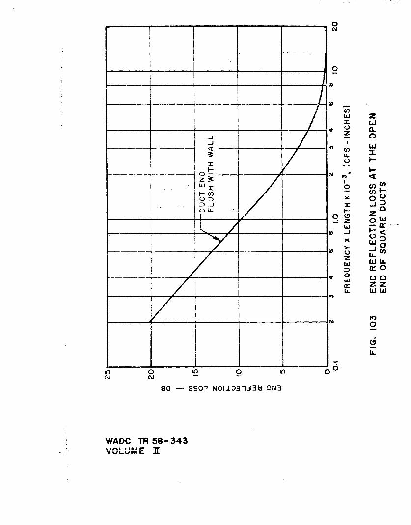
0

00

w~~ C$

-JJ

-~fv7 W

w I

- 0 C

-z

w

zrz

LA. w W

0

I ILA

____I____M ___ __

70 ..--

.~ 60 - - OF, _

V-* RT ICAL OR-O_ HORIZONTAL BAR //w DEFLECTION TYPE,

m ALL ANGLESS50

z !aI 401 - _

_ I \2-PLAINZ PERFORATED

w GRILLE< 30

wI

- J

> 20w

w

0n 10 PWL sL(AVERAGE PWL OF

a 600- 1200, 1200-24007D2400-4800 CPS BANDS)01

400 5 6 8 2 3 440QI00 5000

DUCT AIR VELOCITY IN FT/M IN.

FIG, 104 GRILLE NOISE FOR CORE AREAOF I SQUARE FOOT

WADC TR 58- 343VOLUME 11

1=1 OS NI 8 t O~ALIi.3I00 0 00 00 0 000

N to 00 00 C' 0- NIj 0 0 0 0 u)_

- l n U c 0 CL9f T U)

t o ~LL1J 1. 21 -

0 ww-

z

i f 0 _

ID La

l~~~~~~~~~d~~/ r8 ;t-ACflS~ ~lO A118 'O3dAIAI3I

WAD TR 98-343VOLUM (1

1000

/z

to

v w

U -J

z 4 -j0

u U D W, 0U> a:Ir Z

>I- Li

o~~G 4.Q-C-

00

4- _ to >:-Q:

__ _____ ~ LL 0

CL. 0 (D

(0

(n 0 0

?AVO0131 ZOOO*O 38 80 - 13A31 3flSS38d CJNnos

WADC TR 58-343VOLU ME It

0.020 IN. STEEL (OUTER SKIN)

GLASS FiBER INSULATION1It2 I N.

~0.02 I.SEL

( HO0NE YCo MB J 1IN.-1 1 1 1 : 1 10 1

\,0020 IN. STEEL

FIG.IO7 DETAIL OF DOUBLE WALLCONSTRUCTION IN EXAMPLE.

WADC TIR 58-343VOLUME I[

I-I

w

LJ C~

+E z

E ci, L

E 0

VOLUME +

40'

w i3 A

c'J 0

0 0

z 0-

o I-0 LLJ C

I0 .4 z0

rCr

-- (Y CD wcI z

-o 0-3

00 0uNJ _ _ _ _

Ci5i

00--701

WADC T 58-34VOLUME I

40 _ _BLANKNET,

30- _-_

2IN.

< 0 2ol ''

I IN

wo 4 6 80002 4 6 aIQoO 20.000FREQUENCY (CPS)

FIG. 00 APPROXIMATE TRANSMI SSION- LOSS INCREASE

(ATL) DUE TO ACOUSTICAL BLANKETS.

WADC TR 58-343VOLUME I

IN ECElr~iNCSPA CE

cliMEDIUM

0

LOW

-_301

0 10 20 30 40 50 60TLO O TRANSMITTING WALL-OB

FIG. III Cp , CORRECTION TO TL0 FOR MAXIMUMEFFECT OF STANDING WAVES IN MEDIUM-SIZED RECEIVING SPACE.

WADO TR 58-343VOLUMIVE i

0

0

-201. I I .

005 0.1 020.5 1.0

SW TR A NS M I TINAG SU R FAC E A R EAS2 TOTAL RECEIVING-SPACE SURFACE

FIG. 112 C3 l CORRECTION TO TL0 FOR REVERBERATIONIN LARGE RECEIVING SPACES.

WADO TR 58-343VOLUME 1t

__ ____ ________ ~ 0

-J

Wcf LiZ) -C

z

(f) wZa uiw

o~ Li..

zz

u-

Ld z -

I- w< U) 0 n

IW 0 1

JU,

- z

( 0 0 0

90 Nouno28 SION

WADC TR 58-343VOLUME I[

1401 ..

120- -. I

ROCKET NOISE0 ]MINUS DOUBLE WALL NR

t I SUGGESTED UPWARD05 SPREAD OF MASKING0 6DB/OCTAVE SLOPE

r"~ sj° -N -. [-T,

w

SPEECH PEAK(

40

a- ROCKET NOISEATEAR

20 TI '

I!'0 24 6 8 2 a10O0 1000 10,000

FREQUENCY, CYCLES PER SECOND

FIG, i4 INTELLIGIBILITY OF RECEIVEDSPEECH DURING BOOST

WADC TR 58-343

VOLUME f.

o 110 I00

0

ISENTENCES

D ~80 .. ..

0 -WORDS

0

Uw

zU 40z /U)/

u-0

___ __20 /E: THESE RELATIONS ARE

z APPROXIMATE, AND DEPEND ONTYPE OF MATERIAL AND SKILLOF TALKERS AND LISTENERS.

a-I I0 0.2 0.4 0.6 0.8 1.0

ARTICULATION INDEX

FIG. il5 INTELLIGIBILITY AS A FUNCTIONOF ARTICULATION INDEX.

WADC TR 58- 343

VOLUME 3I

40--

ATTENUATION OF COMBINED HELMET(MOUTH POSITION)

, AND DIFFERENTIAL MICROPHONE

LI pI I

I71

__ _ __ _ _ _ __ __ _ _ __ iI -ATTENUATION OF HELMET

i (EAR POSITION) ORi..... /ATTENUATION OF HEADSET CUSHION

04 6 8100 1000 I0,000

FREQUENCY, CYCLES PER SECOND

FIG. 116 NOISE ATTENUATION OF PRESENT- DAYHIGHAALTITUDE HELMET HEADSET CUSHION

AND DIFFERENTIAL MICROPHONE.

WADC TR 58- 34:3VOLUM E I[

tr'

00

~T40z

ROCK!'<T NOISEL'!AT MACF0PHONE

20-

10010 0:FREJUENCY, CYCLE$ -

FIG.117 NTELLIGI6:LISPEECH DUR

WADC TR 58-343VOLUME M:

Best Available Copy

unclassi fied a d 260955 v - vibrationdata · unclassi fied 260955 a dv ... the effects of rocket...

Documents