unclassified eco/wkp(2016)37 - oecd.org · unclassified eco/wkp(2016)37 organisation de...

Unclassified ECO/WKP(2016)37 Organisation de Coopération et de Développement Économiques Organisation for Economic Co-operation and Development 07-Jul-2016

___________________________________________________________________________________________

_____________ English - Or. English ECONOMICS DEPARTMENT

FORECASTING GDP DURING AND AFTER THE GREAT RECESSION: A CONTEST BETWEEN

SMALL-SCALE BRIDGE AND LARGE-SCALE DYNAMIC FACTOR MODELS

ECONOMICS DEPARTMENT WORKING PAPERS No. 1313

By Patrice Ollivaud, Pierre-Alain Pionnier, Elena Rusticelli, Cyrille Schwellnus and Seung-Hee Koh

OECD Working Papers should not be reported as representing the official views of the OECD or of its member

countries. The opinions expressed and arguments employed are those of the authors.

Authorised for publication by Jean-Luc Schneider, Deputy-Director, Policy Studies Branch, Economics

Department.

All Economics Department Working Papers are available at www.oecd.org/eco/workingpapers

JT03399157

Complete document available on OLIS in its original format

This document and any map included herein are without prejudice to the status of or sovereignty over any territory, to the delimitation of

international frontiers and boundaries and to the name of any territory, city or area.

EC

O/W

KP

(20

16)3

7

Un

classified

En

glish

- Or. E

ng

lish

ECO/WKP(2016)37

2

OECD Working Papers should not be reported as representing the official views of the OECD or of its member countries. The opinions expressed and arguments employed are those of the authors. Working Papers describe preliminary results or research in progress by the author(s) and are published to stimulate discussion on a broad range of issues on which the OECD works. Comments on Working Papers are welcomed, and may be sent to the Economics Department, OECD, 2 rue André-Pascal, 75775 Paris Cedex 16, France. Comment on the Papers is invited, and may be sent to OECD Economics Department, 2 rue André Pascal, 75775 Paris Cedex 16, France, or by e-mail to [email protected]. All Economics Department Working Papers are available at www.oecd.org/eco/workingpapers

This document and any map included herein are without prejudice to the status of or sovereignty over any territory, to the delimitation of international frontiers and boundaries and to the name of any territory, city or area. The statistical data for Israel are supplied by and under the responsibility of the relevant Israeli authorities. The use of such data by the OECD is without prejudice to the status of the Golan Heights, East Jerusalem and Israeli settlements in the West Bank under the terms of international law.

© OECD (2016)

You can copy, download or print OECD content for your own use, and you can include excerpts from OECD publications, databases and multimedia products in your own documents, presentations, blogs, websites and teaching materials, provided that suitable acknowledgment of OECD as source and copyright owner is given. All requests for commercial use and translation rights should be submitted to [email protected]

ECO/WKP(2016)37

3

Abstract/Résumé

Forecasting GDP during and after the Great Recession: A contest between small-scale bridge and

large-scale dynamic factor models

This paper compares the short-term forecasting performance of state-of-the-art large-scale

dynamic factor models (DFMs) and the small-scale bridge models routinely used at the OECD. Pseudo-

real time out-of-sample forecasts for France, Germany, Italy, Japan, United Kingdom and the United States

during and after the Great Recession (2008-2014) suggest that large-scale DFMs are not systematically

more accurate than small-scale bridge models, especially at short forecast horizons. Moreover, DFM

parameters appear to be highly unstable during the Great Recession (2008-2009), making forecast

revisions between successive vintages difficult to explain as revisions cannot be fully attributed to news on

specific groups of indicators. The implication for OECD forecasting practice is that there would be no gain

from switching from the current small-scale bridge models to large-scale DFMs.

JEL classification codes: E37; C53

Keywords: big data, bridge models, dynamic factor models, nowcasting

*****

Prévoir le PIB pendant et après la Grande Récession : Une comparaison des modèles d’étalonnage

de petite taille et des modèles à facteurs dynamiques de grande taille

Cet article compare les performances en prévision à court terme de modèles à facteurs

dynamiques (DFMs) de grande taille standard dans la littérature à celles des modèles d’étalonnage de petite

taille couramment utilisés à l’OCDE pour les exercices de prévision. Des prévisions hors échantillon en

pseudo temps réel pour la France, l’Allemagne, l’Italie, le Japon le Royaume-Uni et les États-Unis pendant

et après la Grande Récession (2008-2014) montrent que les DFMs de grande taille ne sont pas plus

performants, en moyenne, que les modèles d’étalonnage de petite taille, notamment aux horizons les plus

courts. De plus, les paramètres des DFMs sont très instables pendant la Grande Récession, ce qui rend les

révisions des prévisions d’un exercice à l’autre plus difficiles à expliquer et à relier à différents groupes

d’indicateurs. En pratique, nous en concluons que l’OCDE n’aurait pas intérêt, pour ses exercices de

prévision, à abandonner les modèles d’étalonnage de petite taille pour les DFMs de grande taille.

Codes JEL : E37; C53

Mots-clés : mégadonnées, modèles d’étalonnage, modèles à facteurs dynamiques, prévision en temps réel

ECO/WKP(2016)37

4

TABLE OF CONTENTS

FORECASTING GDP DURING AND AFTER THE GREAT RECESSION: A CONTEST BETWEEN

SMALL-SCALE BRIDGE AND LARGE-SCALE DYNAMIC FACTOR MODELS .................................. 5

1. Introduction and main results ............................................................................................................... 5 2. Overview of the bridge and dynamic factor models used for the forecast comparison ........................ 7

2.1 Small-scale bridge models ........................................................................................................... 8 2.2. Large-scale dynamic factor models ........................................................................................... 10

3. A contest between small-scale bridge and large-scale dynamic factor models .................................. 15 3.1 Forecast accuracy during and after the Great Recession (2008Q1-2014Q4) ............................ 16 3.2 Forecast accuracy during the Great Recession (2008Q1-2009Q4) ........................................... 18

BIBLIOGRAPHY ......................................................................................................................................... 22

ANNEX 1. MODEL SELECTION ALGORITHM FOR THE DYNAMIC FACTOR MODELS ............... 24

ANNEX 2. DETAILED RESULTS ON FORECAST ACCURACY OF SIMPLIFIED BRIDGE AND

DYNAMIC FACTOR MODELS .................................................................................................................. 25

ANNEX 3. STANDARD OECD BRIDGE MODELS ................................................................................ 31

ANNEX 4. DECOMPOSITION OF FORECAST REVISIONS INTO CONTRIBUTIONS FROM

MODEL PARAMETERS AND CONTRIBUTIONS FROM INDICATORS ............................................. 34

Tables

Table 1. Indicators included in the (simplified) small-scale bridge models used for the forecast

comparison ................................................................................................................................................... 9 Table 2. Dynamic factor models developed in this paper are more accurate than reference model ......... 12 Table 3. Dynamic factor models in this paper are more accurate than simple benchmarks (2008Q1-

2014Q4) ..................................................................................................................................................... 14 Table 4. Out-of-sample forecast accuracy of dynamic factor models relative to simplified bridge models17 Table 5. Out-of-sample forecast accuracy of Dynamic Factor Models relative to Bridge Models .......... 19

Figures

Figure 1. Decomposition of forecast revisions with the dynamic factor models ....................................... 15 Figure 2. In-sample fit of the simplified bridge and dynamic factor models ............................................. 16 Figure 3. Relative forecast accuracy at different forecast horizons (2008Q1-2014Q4) ............................ 18 Figure 4. Relative forecast accuracy at different forecast horizons (2008Q1-2014Q4) ............................ 20 Figure 5. Contribution of parameter changes to forecast revisions (2008Q1-2009Q4) ............................. 21

ECO/WKP(2016)37

5

FORECASTING GDP DURING AND AFTER THE GREAT RECESSION: A CONTEST

BETWEEN SMALL-SCALE BRIDGE AND LARGE-SCALE DYNAMIC FACTOR MODELS

By Patrice Ollivaud, Pierre-Alain Pionnier, Elena Rusticelli, Cyrille Schwellnus and Seung-Hee Koh1

1. Introduction and main results

1. The failure of forecasters to predict the large downturn in GDP during the global crisis of 2008-

09 and the subsequent large rebound partly reflects the failure of quantitative models to forecast GDP

growth beyond the very near term. Ample evidence suggests that beyond the current quarter neither

structural nor reduced-form models outperform simple rules of thumb such as the constant-growth or

autoregressive benchmarks.2 For the current quarter, reduced-form models that make efficient use of high-

frequency indicators are typically more accurate than simple rules of thumb and as accurate as judgemental

forecasts.3 The evidence thus suggests that even though reduced-form quantitative models are of little help

to predict GDP growth even at fairly short horizons, they may nonetheless be useful tools to track GDP

growth in real time, i.e. to nowcast GDP growth.

2. Nowcasting GDP is highly relevant for macroeconomic policy making, as for most advanced

economies a first estimate of quarterly GDP becomes available only about 4-6 weeks after the end of the

quarter.4 Macroeconomic policy makers therefore monitor a large number of high-frequency indicators of

aggregate economic activity, such as output, sales, sentiment from business tendency and consumer

surveys and financial indicators. Given that the number of potentially relevant indicators is large,

forecasters face the question whether focusing on a small number of series allows separating the signal

from the noise or whether discarded indicators contain relevant information on aggregate economic

activity. A particularly relevant issue is whether forecasters could have done better around the Great

Recession of 2008-09 if they had monitored a larger set of indicators, including high-frequency indicators

measuring the state of the financial system.

3. This paper compares short-term GDP forecasts for selected advanced economies from small-

scale bridge models – which focus on a small number of carefully selected indicators – with those from

1. The authors are members of the OECD Economics Department (Ollivaud, Rusticelli, Schwellnus and Koh)

and the OECD Statistics Directorate (Pionnier). They would like to thank Catherine Doz (Paris School of

Economics) for invaluable input at the initial phase of this project, as well as Marta Banbura (ECB),

Laurent Ferrara (Banque de France), Dave Turner for helpful discussions and Veronica Humi for editorial

assistance.

2. Recent contributions showing that beyond the current quarter GDP forecasts based on constant-growth or

autoregressive benchmarks are at least as accurate as those based on Dynamic Stochastic General

Equilibrium models and Factor Models include Edge et al. (2010), Edge and Gurkaynak (2010) and Wang

(2009). A recent survey of the forecasting performance of a range of structural and reduced-form models

can be found in Chauvet and Potter (2013).

3. Sédillot and Pain (2003) show for G7 countries that for the current quarter linear models incorporating

information from key monthly indicators outperform constant growth and autoregressive benchmarks while

Banbura et al. (2013) show for the United States that at short forecast horizons Dynamic Factor Models

based on a large number of monthly indicators provide similar forecast accuracy as the Survey of

Professional Forecasters.

4. Strictly speaking, GDP is backcast between the end of the quarter and the official GDP release.

ECO/WKP(2016)37

6

large-scale dynamic factor models – which are specifically designed to deal with data-rich environments.5

The two models deal with high collinearity between macroeconomic time series in a fundamentally

different way; while the bridge models use a pre-selection procedure to retain only a small number of

monthly indicators in the estimated equation, the dynamic factor models in this paper extract a small

number of latent common factors from a large number of monthly indicators. Typically, the bridge models

are based on around 10 key indicators whereas the dynamic factor models are based on 60-80 indicators.

4. This paper complements and extends existing studies on the forecast accuracy of large-scale

dynamic factor models along the following dimensions:

The small-scale bridge models in this paper are simplified versions of those routinely used in the

OECD Economics Department rather than the more rudimentary models typically underlying

forecast evaluation exercises in the academic literature.6 The OECD bridge models combine

forecasts from multivariate models based on key hard and survey indicators whereas the

academic literature typically uses naive univariate models, which unduly skews forecast

comparisons in favour of dynamic factor models.7

A special focus of the forecast comparison between small-scale bridge models and dynamic

factor models is on the global crisis of 2008-09. A number of studies report a particularly large

increase in forecast accuracy of dynamic factor models relative to simple benchmarks during

periods of high volatility (D’Agostino et al., 2006; Godbout and Lombardi, 2012). This paper

analyses whether the forecast accuracy of dynamic factor models relative to bridge models

increased during the global crisis of 2008-09.

Comparisons are based on forecasting models for six large advanced economies (France,

Germany, Italy, Japan, the United Kingdom and the United States) rather than a single country,

which enables an assessment of whether one class of model systematically outperforms the other

or whether relative forecast performance is country-specific.

5. The main results and implications for the forecasting process in the OECD Economics

Department are as follows:

Over all forecast horizons (from six months ahead to the eve of the GDP release), large-scale

dynamic factor models based on at least 30 and up to 130 indicators do not significantly

outperform small-scale bridge models based on 3-4 generic monthly indicators (e.g. industrial

production, household consumption).

5. For a review of the literature on dynamic factor models, see Barhoumi et al. (2013a).

6. See, for instance, Banbura et al. (2013), Barhoumi et al. (2008) and Girardi et al. (2014).

7. The lower forecast accuracy of bridge models relative to dynamic factor models reported by Banbura et al.

(2013), for instance, is likely to reflect the fact that 23 monthly indicators with widely differing predictive

power for quarterly GDP growth are forecast with separate univariate autoregressions that do not account

for dynamic relationships across indicators and that receive the same weight in the final bridge model

forecast. For instance, monthly industrial production is forecast using a univariate autoregression that does

not account for the fact that more timely survey indicators are leading indicators of industrial production.

Moreover, industrial production receives the same weight in the final GDP forecast as indicators with

significantly lower predictive power, such as the three-month interest rate.

ECO/WKP(2016)37

7

Over all forecast horizons, no model systematically outperforms the other for all countries,

implying that the most accurate nowcasts would be obtained by adopting a country-specific

modelling approach.

Large-scale DFMs tend to be more accurate than the small-scale bridge models at longer forecast

horizons but the opposite is true at shorter forecast horizons.

The above results on relative forecast accuracy hold both for the entire evaluation period

2008Q1-2014Q4 and the for Great Recession (2008Q1-2009Q4), but during the Great Recession

differences in forecast accuracy across the two model classes are marginal relative to the size of

the absolute forecast errors.

Combining forecasts of small-scale bridge models and large-scale dynamic factor models does

not result in significant gains in forecast accuracy relative to the standalone models.

Large-scale dynamic factor models are very unstable during the Great Recession, making it

impossible to fully attribute forecast revisions to specific groups of indicators. Small-scale bridge

models are more stable over the same period.

Given that the use of dynamic factor models would imply insignificant gains in forecast accuracy

and parameter instability during periods of high volatility such as the Great Recession, the results

in this paper suggest that small-scale bridge models should remain the main tool to inform short-

term GDP forecasts of country experts at the OECD. The large-scale dynamic factor models may

nonetheless provide a check on the plausibility of the forecasts from the small-scale bridge

models.

6. The remainder of the paper is structured as follows. Section 2 provides an overview of the small-

scale bridge models and the large-scale dynamic factor models used for the forecast comparison. Section

2.1 describes the specification and estimation of the small-scale bridge models, emphasising that the

specification is generic in terms of included indicators and does not aim to maximise forecast accuracy

over specific periods. Section 2.2 describes the specification and estimation of the large-scale dynamic

factor models and shows that forecast accuracy is sensitive to the set of selected indicators and the number

of factors. Section 3 analyses forecast accuracy of the large-scale dynamic factor models relative to the

small-scale bridge models, showing that, on balance, differences in forecast accuracy are negligible.

Special emphasis is placed on forecast accuracy during the global crisis of 2008-09 and the subsequent

rebound. The results suggest that the marginally higher forecast accuracy of the dynamic factor models

several months ahead of the GDP release comes at the cost of larger parameter instability.

2. Overview of the bridge and dynamic factor models used for the forecast comparison

7. This section describes the specification and estimation of the small-scale bridge and large-scale

dynamic factor models underlying the forecast comparisons below. Models extracting information from

high-frequency indicators to forecast quarterly GDP face three main methodological challenges: high

collinearity across macroeconomic time series, staggered data releases and mixed frequencies. In the

bridge models underlying the forecast comparison below, the collinearity issue is addressed by selecting a

small set of key indicators and averaging across forecasts. In the dynamic factor models, a small number of

latent factors is extracted from a large set of collinear indicators, which amounts to averaging across

indicators rather than forecasts. In the bridge models, staggered data releases are addressed by simple re-

alignment of the monthly data series in such a way that a balanced dataset is obtained, whereas in the

dynamic factor model the Kalman filter allows to compute the latent factors even when some monthly

indicators are missing, taking only into account the existing information. Both models address mixed

ECO/WKP(2016)37

8

frequencies by linking the quarterly GDP growth rate to quarterly averages of the indicators or factors. In

this sense, the dynamic factor approach can be seen as a bridge model based on factors.8

2.1 Small-scale bridge models

8. The bridge models routinely used in the OECD Economics Department to monitor short-term

GDP developments for the G7 countries take the following generic form (Sédillot and Pain, 2003;

Mourougane, 2006):

𝑋𝑡 = 𝑘 + ∑ 𝐴𝑝𝑋𝑡−𝑝 + Γ𝑡𝑃𝑝=1 (1)

𝑦𝑡 = 𝑐 + ∑ ∅𝑙𝑦𝑡−𝑙𝐿𝑙=1 + ∑ ∑ 𝛽𝑖𝑗𝑥𝑖,𝑡−𝑗

𝑄𝐽𝑗=0

𝐼𝑖=1 + 𝑢𝑡 (2)

where equation (1) is the auxiliary monthly model to forecast the monthly indicators and equation (2) is the

quarterly bridge equation. The auxiliary model is a vector autoregression (VAR), where 𝑋𝑡 =

(𝑥1,𝑡, … , 𝑥𝑁,𝑡)′ is a vector of N monthly indicators and 𝐴𝑝 is a conformable matrix of coefficients.9 To

reduce the risk of inefficient estimates due to high dimensionality of the monthly VAR and limited degrees

of freedom, Bayesian methods are used to shrink the number of estimated parameters.10

The parameters of

the quarterly bridge equation (c, ∅𝑙 , 𝛽𝑖𝑗) are obtained by regressing quarterly GDP growth 𝑦𝑡 on a constant,

lagged values of GDP growth, and contemporaneous and lagged values of monthly indicators aggregated

to the quarterly frequency (𝑥𝑖,𝑡−𝑗𝑄

).

9. The first step in dealing with high collinearity is to carefully select a small number of key

indicators. For the purposes of the forecasting contest below the suite of small-scale bridge models

routinely used in the OECD Economics Department is simplified to include only a small number of generic

indicators. Some of the country models currently used in the OECD Economics Department includes

housing and financial indicators that were added in the wake of the global crisis of 2008-09. Given that

these indicators were included with hindsight, they may unduly skew forecast performance during the

crisis in favour of the small-scale bridge models. Even though the dynamic factor models typically include

a number of housing and financial indicators, the forecasting contest below therefore reports the results for

simplified versions of the small-scale bridge models that include only industrial production, household

8. A further approach to short-term GDP forecasting based on high-frequency indicators is the mixed-data

sampling (MIDAS) model developed by Ghysels et al. (2004). In contrast to approaches based on quarterly

bridge equations, mixed-data sampling allows the modelling of time series of different frequencies without

averaging the high-frequency series. Staggered data releases can be dealt with by re-aligning indicator

series in such a way that a balanced dataset is obtained, e.g. if one indicator becomes available one month

before all others all other indicators are shifted forward by one month (Altissimo et al., 2006). The

distributed lag structure of the model is used to obtain direct forecasts of GDP several quarters ahead

without resorting to an auxiliary model. Mixed-data sampling can address the high collinearity of

macroeconomic time series by either combining forecasts from different indicator models or by combining

mixed-data sampling with factor analysis.

9. Note that I indicators are used to forecast GDP in the quarterly bridge equation (equation 2) whereas N

indicators (𝑁 ≥ 𝐼) may be used in the auxiliary model to forecast the monthly indicators (equation 1).

10. Sims-Zha Normal-Wishart priors on the parameters are chosen.

ECO/WKP(2016)37

9

consumption, and business and consumer confidence.11

The results for the standard suite of bridge models

are reported in Annex 3.

10. The second step in dealing with high collinearity is to take the simple average across forecasts

from a pure hard indicator model, a survey indicator model and a mixed indicator model so that each

model implicitly receives a fixed weight of one third.12

The pure hard indicator models typically include

industrial production and household consumption in the quarterly bridge equations of the simplified

models; the pure survey indicator models typically include a PMI and household confidence; and the

mixed indicator models include a subset of the indicators included in the pure hard and survey models

(Table 1). Only indicators that are statistically significant in the quarterly bridge equations or that raise

forecast accuracy prior to the sample period used for the contest between bridge and dynamic factors

models are included in the simplified bridge models.13

For most countries and sub-models the estimation

sample starts in the first half of the 1990s.

Table 1. Indicators included in the (simplified) small-scale bridge models used for the forecast comparison

Note:

1. Included only in monthly VAR.

11. If monthly household consumption is not available, it is replaced by a proxy indicator such as retail sales or

car registrations. Monthly indicators that are insignificant at the 10% level in the quarterly bridge equation

but reduce root mean squared forecast error of pseudo-out-of-sample forecasts over the period 2003Q1-

2007Q4 are included in the monthly VAR only.

12. The bridge model routinely used in the OECD Economics Department uses a weighted average of the

forecasts from the three sub-models, with the model weights based on relative forecast accuracy of pseudo-

out-of sample forecasts over the recent past and computed for each forecast horizon separately. As more

up-to-date hard indicators become available this tends to increase the weight of the hard indicator model

relative to the survey- and mixed-indicator models. For simplicity and given that for some sub-models the

pre-evaluation period is too short to precisely estimate weights by forecast horizon, the forecast

comparison in Section 3 is based on the simple average of the sub-models, although this may reduce

overall forecasting performance of the bridge model.

13. The standard bridge models additionally include a few other indicators such as house price indices,

inventories, industrial orders or sector-specific PMIs (see Annex A3).

Country Model Start Lag of GDP Included in quarterly bridge equation

France Soft 1990q1 No Business confidence (recent output), Household confidence¹

Hard 1990q1 Yes Industrial production, Household Consumption

Mixed 1990q1 Yes Industrial production, Household Consumption, Business confidence (recent output)¹, Consumer confidence¹

Germay Soft 1996q2 Yes Markit manufacturing PMI, Ifo consumer confidence

Hard 1994q2 No Industrial production, Retail sales excluding cars

Mixed 1996q2 Yes Industrial production, Retail sales excluding cars, Markit manufacturing PMI, Ifo consumer confidence¹

Italy Soft 1997q3 No Markit manufacturing PMI

Hard 1996q3 Yes Industrial production, Car registration

Mixed 1996q2 No Industrial production, Car registration, Markit manufacturing PMI¹

Japan Soft 2001q4 No Markit manufacturing PMI

Hard 1990q1 No Industrial production, Real living expenditure index

Mixed 1990q1 No Industrial production, Real living expenditure index, Markit manufacturing PMI¹

United Kingdom Soft 1992q1 Yes Markit manufacturing PMI, EC consumer confidence

Hard 1990q1 Yes Industrial production, Retail sales

Mixed 1990q1 Yes Industrial production, Retail sales, EC consumer confidence

United States Soft 1990q1 No ISM manufacturing PMI, Consumer confidence

Hard 1990q2 Yes Industrial production, Private consumption

Mixed 1990q2 Yes Industrial production, Private consumption, ISM manufacturing PMI¹, Consumer confidence¹

ECO/WKP(2016)37

10

11. Staggered indicator releases are dealt with by re-aligning monthly indicators before estimation of

the auxiliary VAR model and restoring observed publication delays thereafter. Before estimation, those

monthly indicators which are not available for a given month are shifted forward until all indicators are

aligned.14

After estimation of the auxiliary VAR and once out-of-sample forecasts at suitable horizons are

obtained, the monthly series are shifted back to restore observed publication delays. While it is possible to

cast the VAR in state-space form and to use the Kalman filter to deal with missing indicator values at the

end of the sample (Matheson, 2012), pseudo-out of sample forecasts suggest that using the horizontal re-

alignment procedure to address staggered data releases yields similar accuracy of GDP forecasts as the

Kalman filter at all forecast horizons.

12. The small-scale bridge models used in the OECD Economics Department generally outperform

quarterly GDP forecasts of simple benchmark models when some monthly indicators for the quarter are

available and they provided a fairly accurate real-time signal on GDP growth during the global crisis of

2008-09 (Sédillot and Pain, 2003; Pain et al., 2014). The bridge models are highly tractable, in the sense

that only a small number of key indicators are included and parameter estimates are fairly stable so that

forecast revisions can easily be traced to individual indicators.15

However, at more distant forecast

horizons, the small-scale bridge models do not systematically outperform simple benchmarks, suggesting

that most monthly indicators have only weak predictive power for GDP growth beyond the current quarter.

For instance, during the global crisis, forecasts made in March 2009 failed to predict the upturn for the

second and third quarters of 2009.

2.2. Large-scale dynamic factor models

13. Factor models address the collinearity issue by extracting a small number of factors from a large

set of indicators. The large-scale dynamic factor models used in this paper are based on the methodology

developed by Giannone et al. (2008) and take the following generic form: 16

𝑋𝑡 = Λ𝐹𝑡 + ϵ𝑡 (3)

𝐹𝑡 = ∑ 𝐵𝑝𝐹𝑡−𝑝 + 𝜂𝑡𝑃𝑝=1 (4)

where 𝑋𝑡 is a vector of N monthly indicators; 𝐹𝑡 = (𝑓1,𝑡, … , 𝑓𝑟,𝑡)′ is a vector of r latent factors; Λ is a

(𝑁 × 𝑟) dimensional matrix of factor loadings; ϵ𝑡 is a vector of idiosyncratic disturbances; 𝐵𝑝 are (𝑟 × 𝑟)

dimensional coefficients matrices and 𝜂𝑡 is a vector of factor innovations. The idiosyncratic disturbances

are assumed to be uncorrelated with the factor innovations at all leads and lags, i.e. 𝐸(𝜖𝑖,𝑡𝜂𝑗,𝑡−𝑘) = 0 for

all i, j and k. While in the exact factor model, the elements of 𝜖𝑡 are assumed to be mutually uncorrelated at

14. For instance, if PMIs are available until May and industrial production is available until March, all values

for industrial production are shifted forward by two months and the monthly VAR can be estimated using

all available information. Once the forecasts for industrial production have been generated, all values for

industrial production are shifted backward by two months.

15. For instance, higher monthly industrial production growth than forecast by the auxiliary model is typically

.associated with a positive GDP revision, as the estimated coefficient on industrial production in the

quarterly bridge equation is positive.

16. This model has been applied to other countries, including the euro area (Angelini et al., 2011), France

(Bessec and Doz, 2013), Germany (Antipa et al. 2012), Ireland (D’Agostino et al., 2008), Japan (Godbout

and Lombardi, 2012) and New Zealand (Matheson, 2010). Matheson (2012) estimates this model for 32

advanced and emerging economies. GDP nowcasts and short-term forecasts based on this approach have

been shown to outperform constant-growth, autoregressive and simple bridge equation benchmarks.

ECO/WKP(2016)37

11

all leads and lags, i.e. 𝐸(𝜖𝑖,𝑡𝜀𝑗,𝑡−𝑠) = 0 for all s if i ≠ j, in the approximate factor model used in this paper

it is allowed for correlation between the elements of 𝜖𝑡 (both in cross-section and along the time

dimension) but it is assumed that the contribution of the idiosyncratic disturbances to the dynamics of the

indicators is negligible relative to the contribution of the common factors. Equation (3) links the monthly

indicators to a small number of r (𝑟 ≪ 𝑁) latent factors and equation (4) is a P-order VAR in the latent

factors.

14. The latent dynamic factors can be estimated following the two-step method proposed by Doz et

al. (2011). In a first step, estimates of Λ, 𝐹𝑡 and ϵ𝑡 in equation (3) are obtained by Principal Components

Analysis (PCA) on a balanced dataset of monthly indicators and estimates of (𝐴1…𝐴𝑃) and 𝜂𝑡 by

estimating a VAR in the estimated 𝐹𝑡 (equation 4). Noting that the dynamic factor model may be cast as a

linear state-space model, with (3) being the measurement equation and (4) the state equation, the factors

are then re-estimated using the Kalman filter and smoother. While the principal components average across

indicators only, the Kalman filter and smoother additionally average across time. The averaging across

time smoothes the principal components, which improves estimates if the signal from the latent dynamic

factors is persistent and if substantial noise remains after principal components analysis (Stock and

Watson, 2011).

15. Alternatively, the latent dynamic factors can be estimated by Quasi-Maximum Likelihood

(QML), which involves using the factor estimates from the two-step estimation procedure as initial values

and iterating using the Expectation-Maximisation (EM) algorithm until convergence is achieved. 17

Evidence based on generated data suggests that QML estimates of the latent dynamic factors approximate

the true factors more precisely than estimates based on the two-step procedure described above (Doz et al.,

2012; Banbura and Modugno, 2014).

16. Staggered data releases are addressed using the Kalman filter and smoother, which, additionally

to providing more efficient estimates of the latent factors for all months covered by the principal

components analysis, also provides estimates of the underlying factors when some monthly indicators are

missing.

17. The issue of mixed frequencies is addressed by first using the VAR in equation (4) to forecast

monthly factors and then substituting quarterly averages of the forecast factors (𝑓1,𝑡𝑄 , … , 𝑓𝑟,𝑡

𝑄) into the

following quarterly equation estimated by ordinary least squares:18

𝑦𝑡 = 𝑐 + ∑ φ𝑙𝑦𝑡−𝑙 + ∑ 𝛾𝑖𝑓𝑖,𝑡𝑄𝑟

𝑖=1 + 𝑢𝑡 𝐿𝑙=1 (5)

Instead of using the state-space model to forecast the monthly factors, forecasts for quarterly GDP growth

could be obtained by directly forecasting GDP growth using lags of the estimated factors. For instance,

forecasts of dynamic factors could have been generated up to the end of the quarter for which the most

recent monthly indicators are available. Nowcasts could then be obtained by using a bridge equation

linking current GDP growth to current factors and forecasts by an equation linking current GDP growth to

the first lag of the quarterly averages of the factors. In practice, however, accuracy of GDP forecasts based

17. Note that the QML procedure applied in this paper (Banbura and Modugno, 2014) allows estimating model

parameters on datasets of monthly indicators starting at different dates, which is very relevant in practice.

18. Non-stationary indicators enter the dynamic factor model either as three-month growth rates or as three-

month differences. All indicators are standardised with mean equal to 0 and variance equal to 1. All r static

factors are included in the quarterly equation. Including only statistically significant factors does not

appreciably affect forecast accuracy.

ECO/WKP(2016)37

12

on factor forecasts is similar to that based on direct forecasts and has the additional advantage that forecast

revisions are not driven by differences in parameters of the quarterly equations.

18. To validate the computer codes developed for this paper, out-of-sample forecasts were compared

with those obtained by Bessec and Doz (2013) for France. Based on the identical dataset obtained from the

authors, identical model specification and the use of the two-step estimator developed by Doz et al. (2011),

the dynamic factor model in this paper almost perfectly replicates the authors’ results (Table 1, Rows 1 and

2).19

The forecast error of the models in this paper is reduced relative to the reference model by computing

3-month growth rates or 3-month differences instead of monthly growth rates or monthly differences of

non-stationary indicators as in Bessec and Doz (2013). These transformations ensure that the simple

average of monthly factors over a quarter corresponds to a quarterly growth rate (Table 1, Row 3).20

A

further reduction in forecast error is achieved by estimating the model by quasi-maximum likelihood rather

than the two-step estimator (Table 1, Row 4).21

Therefore, the final dynamic factor specification chosen for

the comparison with the bridge models in this paper is even more accurate than the state-of-the-art model

developed by Bessec and Doz (2013).

Table 2. Dynamic factor models developed in this paper are more accurate than reference model

Root mean squared error (2000Q1-2009Q3)

Note: Root mean squared error in Bessec and Doz (2013) is annualised by multiplying reported non-annualised values by 4. Row (1) reports the results obtained by using the VAR model to forecast the factors, which is referred to as Method (1) in Bessec and Doz (2013).

Source: Bessec and Doz (2013), including their original dataset; OECD Economic Outlook database (May 2015); Datastream; and OECD calculations.

19. The composition of the initial datasets is harmonised as much as possible across countries. For

France, Germany, Italy and the United Kingdom survey indicators are taken from the Joint Harmonised EU

Programme of Business and Consumer Surveys (European Commission, 2016). Aside from the United

States, financial and international environment variables are common to all countries. For the United

19. In a private exchange, the authors indicated that the difference at one month before the publication of GDP

reflects an error in the computer code used by Bessec and Doz (2013).

20. For European countries, the computation of three-month growth rates or three-month differences of non-

stationary indicators (e.g. industrial production) also allows alignment of the transformed indicators with

business tendency survey variables. For instance, managers of manufacturing firms in the European Union

are asked how their production developed over the past three months and is expected to develop over the

next three months (European Commission, 2016). Therefore, this strategy is preferred to the alternative of

computing monthly growth rates or monthly differences of non-stationary indicators and a weighted

average of monthly factors.

21. Row (2) of Table 1 is based on the assumption that in month 0 GDP for the forecast quarter is available for

the estimation of the model parameters, which is consistent with the assumption in Bessec and Doz (2013).

Rows (3) and (4) are based on the more realistic assumption that in month 0 GDP is not available for the

estimation of the model parameters.

Months to publication of GDP 0 1 2 3 4 5 6 Mean

(1) Bessec and Doz (2013) 0.88 0.96 1.56 1.60 1.88 2.00 2.20 1.60

(2) Replication 0.88 1.20 1.52 1.56 1.84 1.92 2.24 1.60

(3) (2) + 3-month growth rates of indicators 1.01 1.08 1.32 1.32 1.72 1.60 1.76 1.40

(4) (3) + QML 0.99 1.04 1.36 1.16 1.60 1.36 1.56 1.28

ECO/WKP(2016)37

13

States, all indicators are taken from the FRED-MD database maintained by the Federal Reserve Bank of St.

Louis in order to follow the literature as closely as possible. This database updates the classical Stock-

Watson database of monthly indicators for the United States (MacCracken and Ng, 2015). Japan is a

second specific case because tendency surveys and real indicators available for this country often do not

have an equivalent in other countries.22

20. An identical model selection algorithm is applied to all countries. The algorithm selects the

subset of monthly indicators and the number of factors in the state-space model that maximises out-of-

sample forecast accuracy over 2003Q1-2007Q4. Indeed, the inclusion of more indicators does not

necessarily imply better forecasts (Boivin and Ng 2006, Bai and Ng 2008). More precisely, the model

selection algorithm evaluates pseudo-out-of-sample forecasts over 2003Q1-2007Q4 for various

permutations of reduced monthly indicator sets and numbers of factors, where the reduction of the initial

monthly indicator sets is based on statistical significance in univariate regressions of GDP on monthly

indicators (see Annex 1 for further details on the model selection algorithm). Basing indicator selection

and model specification on out-of-sample forecast accuracy on the pre-crisis period puts the dynamic

factor models on par with the bridge models, which include a small number of generic indicators not

specifically geared towards maximising forecast accuracy over the evaluation period 2008Q1-2014Q4.

21. Streamlining datasets as described above, setting a number of factors based on out-of-sample

forecasting performance on a training sample rather than information criteria (Bai and Ng, 2002) and

quasi-maximum likelihood estimation maximises forecast accuracy for most countries (Table A2.1).

Forecast accuracy is evaluated as the Root Mean Squared Error (RMSE) of pseudo-real time forecasts at

horizons of 0 to 6 months before the publication of quarterly GDP.23

Over the evaluation period (2008Q1-

2014Q4), the specification of the dynamic factor models based on forecast accuracy over the training

sample (2003Q1-2007Q4) is fixed and forecasts at each horizon are generated using the same model. Only

model parameters are sequentially re-estimated at each iteration.

22. The dynamic factor specifications chosen for the comparison with the bridge models are more

accurate over 2008Q1-2014Q4 than simple autoregressive and constant-growth benchmarks, especially at

short forecast horizons (Table 3). While for some countries the autoregressive benchmark is only

marginally less accurate than the dynamic factor models six months ahead of the GDP release, the dynamic

factor models become increasingly more accurate as monthly indicators for the forecast quarter become

available. In the month of the GDP release, the dynamic factors models are typically 30-40% more

accurate than the autoregressive benchmarks. The superiority of the dynamic factor models is even more

pronounced relative to constant growth benchmarks, which reflects the fact that constant GDP is a

particularly poor forecast during periods of large GDP growth volatility. Overall, these results are

qualitatively and quantitatively consistent with previous studies showing that at very short forecast

horizons dynamic factor models outperform simple benchmarks by a large margin.

22. The initial datasets include 62 monthly indicators for Japan, 70 for Italy, 75 for France, 79 for the UK, 86

for Germany and 133 for the United States (see Annex Table A2.1).

23. The out-of-sample forecasts are generated using revised data accessed in June 2015 for quarterly GDP and

monthly indicators.

ECO/WKP(2016)37

14

Table 3. Dynamic factor models in this paper are more accurate than simple benchmarks (2008Q1-2014Q4)

Panel A: Ratio of out-of-sample RMSE of dynamic factor model to out-of-sample RMSE of AR(1) benchmark

Panel B: Ratio of out-of-sample RMSE of dynamic factor model to out-of-sample RMSE of constant growth benchmark

Note: *, **, *** indicate that the difference in forecast accuracy between the two models is statistically significant at the 10%, 5% and 1% levels. Source: OECD Economic Outlook database (May 2015); Datastream; and OECD calculations.

23. An advantage of the state-space model is that forecast revisions can be traced to individual

indicators and grouped into contributions from broader groups of indicators (Banbura and Modugno,

2014). Note that we rely on the same model specification for all forecast horizons, only allowing for model

parameters to evolve over time, precisely in order to be able to decompose forecast revisions. The

decomposition involves computing how newly released monthly indicators influence the estimates of latent

factors. If the parameters of the state-space model and the quarterly bridge equation are unchanged,

revisions to the quarterly GDP forecast can be fully assigned to news on the monthly indicators. For

instance, if newly released survey indicators turn out more positive than forecast by the model before the

data release, then the contribution of this news’ release will be positive and survey indicators will

contribute positively to the revision of the quarterly GDP forecast.

24. Decompositions of forecast revisions over 2008Q1-2014Q4 suggest that surveys, financial and

international indicators drive forecast revisions at longer horizons while hard indicators play a more

prominent role at shorter horizons (Figure 1). Surveys, financial and international indicators appear to

provide a valuable signal on GDP growth when hard indicators are unavailable, which reflects their

timeliness and, in some cases, their forward-looking nature. However, these indicators appear to add less

information on GDP growth once hard indicators for the forecast quarter become available. Changes in

model parameters contribute less to forecast revisions than news on indicators but nonetheless play a

significant role, which mainly reflects large changes in parameters during the Great Recession (2008Q1-

2009Q4). This finding is further investigated in Section 3.

Months to GDP release 0 1 2 3 4 5 6 Mean

France 0.50** 0.55* 0.63 0.64 0.78 0.90 0.82 0.69

Germany 0.64 0.65 0.68 0.68 0.72 0.74 0.83 0.71

Italy 0.46 0.59 0.75 0.72 0.80 0.88 0.86* 0.72

Japan 0.53* 0.54* 0.62 0.72 0.83 1.08 1.10 0.77

United Kingdom 0.67 0.74 0.94 0.78 0.83 0.91 0.82 0.81

United States 0.77 0.74 0.75 0.70 0.90 0.95 0.9 0.82


France 0.47*** 0.52** 0.59*** 0.59* 0.73* 0.85 0.70* 0.64**

Germany 0.60* 0.61* 0.63 0.55 0.58 0.59 0.61 0.60

Italy 0.49* 0.63 0.80 0.69* 0.77* 0.85* 0.73* 0.71*

Japan 0.46*** 0.47*** 0.54** 0.53** 0.61** 0.79*** 0.75*** 0.59***

United Kingdom 0.67* 0.74 0.95 0.75 0.80 0.87 0.70 0.78

United States 0.71*** 0.67*** 0.68*** 0.61 0.78 0.82* 0.76 0.72**

ECO/WKP(2016)37

15

Figure 1. Decomposition of forecast revisions with the Dynamic Factor Models

2008Q1-2014Q4

Note: The share of each component in Figure 1 is computed as the ratio of the average absolute contribution of this component to the sum of the absolute contributions of all components. “Other indicators” include financial and international indicators, as well as contributions from past GDP growth releases when the quarterly equation linking GDP growth with factors includes GDP lags (only relevant for France and Germany, see Annex Table A1). Contributions to forecast revisions are computed as contributions from news on the monthly indicators, using the same methodology as Banbura and Modugno (2014).

Source: OECD Economic Outlook database (May 2015); Datastream; and OECD calculations.

3. A contest between small-scale bridge and large-scale dynamic factor models

25. This section pits the small-scale simplified bridge models against the large-scale dynamic factor

models described in the previous section. Particular attention is paid to not inadvertently favouring one

model over the other. Neither the bridge models nor the dynamic factor models maximise forecast

accuracy specifically over the evaluation period. Indicator selection is based on the pre-evaluation period,

with the set of indicators included in the bridge models constrained to key indicators such as industrial

production, retail sales as well as business and consumer confidence. Preference is given to simple and

transparent specifications, with the simple average of the hard, survey and mixed models serving as the

bridge model forecast rather than the weighted average based on past forecast errors.

26. Over the period 1990Q1-2007Q4, the simplified bridge models based on 3-4 generic indicators

explain a similar share of the variation of GDP growth as the dynamic factor models that are based on up

to 130 indicators (Figure 2).24

Although for some countries, including France, the United Kingdom and the

United States, the dynamic factor models appear to track quarterly GDP growth more accurately in sample

over 1990Q1-2007Q4, several months ahead of official GDP releases, taking into account staggered

24. In the case of DFMs, adjusted R²s over 1990Q1-2007Q4 are computed from regressions of quarterly GDP

growth on a constant, quarterly factors and potentially one lag of quarterly GDP growth. The number of

factors, the composition of the monthly information sets and the inclusion of a lag of GDP growth are

chosen so as to maximise out-of-sample forecast performance over 2003Q1-2007Q4 (see detailed

specifications in Table A1).

In the case of simplified bridge models, in-sample fits of hard, soft and mixed models over 1990Q1-

2007Q4 are averaged so as to compute the corresponding adjusted R²s.

0

10

20

30

40

50

60

70

80

90

100

0

10

20

30

40

50

60

70

80

90

100

M-6 to M-3 M-3 to M-0 M-6 to M-3 M-3 to M-0 M-6 to M-3 M-3 to M-0 M-6 to M-3 M-3 to M-0 M-6 to M-3 M-3 to M-0 M-6 to M-3 M-3 to M-0

France Germany Italy Japan United Kingdom United States

Survey indicators Hard indicators Other indicators Model parameters

ECO/WKP(2016)37

16

released of monthly data, and out of sample over 2008Q1-2014Q4, the bridge models may nonetheless

forecast GDP growth more accurately than the dynamic factor models.

Figure 2. In-sample fit of the Simplified Bridge and Dynamic Factor Models

Adjusted R2, 1990Q1-2007Q4


3.1 Forecast accuracy during and after the Great Recession (2008Q1-2014Q4)

27. Forecast accuracy over the period 2008Q1-2014Q4 is evaluated based on pseudo-real time

forecasts. A first set of pseudo-real time forecasts is obtained by generating a dataset that mirrors data

availability six months ahead of the release of quarterly GDP for 2008Q1.25

For countries for which GDP

for the first quarter is released in May (France, Germany, Italy and Japan), this corresponds to monthly

data availability at the end of November 2007. Publication delays for monthly indicators are fully

accounted for. For example, survey indicators are typically available one or two months before most hard

indicators for the same period, so if survey indicators in the generated dataset are available up to

November, then most hard indicators will only be available up to September or October. The bridge and

dynamic factor models are then used to produce a first GDP forecast for 2008Q1, after what the dataset is

extended by one month. This process is iterated forward until a full set of pseudo-real time GDP forecasts

at horizons of 6 to 0 months ahead of the publication date of GDP are obtained for the period

2008Q1-2014Q4, with model parameters re-estimated at each iteration.26

Thus for each of the 28 quarters

25. Reconstructing real-time vintages of monthly indicators and GDP growth for each month of the evaluation

period is impossible because indicator vintages are unavailable and only two vintages of GDP releases per

year are available in the OECD Economic Outlook databases. In any case, using real-time data would likely

have only a marginal effect on the comparison across models.

26. Model parameters are re-estimated at each iteration, but the choice of model (selected indicators, number

of underlying factors, estimation method) is kept constant and based on out-of-sample forecasting

performance on the 2003Q1-2007Q4 training sample.

Forecasts “0 month ahead” are computed with all monthly indicators available at the end of month m, but

without knowing quarterly GDP growth released at month m. Hence, these forecasts are truly out-of-

sample forecasts of GDP growth. Similarly, forecasts “three months ahead” are computed without knowing

0

0.1

0.2

0.3

0.4

0.5

0.6

0.7


Bridge model Dynamic factor model

ECO/WKP(2016)37

17

over the forecast comparison period 2008Q1-2014Q4, there are seven pairs of competing forecasts. Results

are based on the root mean squared error (RMSE) as a measure of forecast accuracy.

28. Differences in forecast accuracy between the large-scale dynamic factor models and the small-

scale bridge models are typically small and statistically insignificant.27

Aside from France, differences in

forecast errors over all forecast horizons between the dynamic factor models and the simplified bridge

models that include 3-4 generic indicators only are on average around 10% or below (Table 4). Accuracy is

also not systematically higher for large-scale DFMs. While average DFM forecast errors over all forecast

horizons are lower for France, Japan and the United Kingdom, they are higher for Germany, Italy and the

United States.28

Table 4. Out-of-sample forecast accuracy of dynamic factor models relative to simplified bridge models (2008Q1-2014Q4)

Ratio of out-of-sample RMSE of dynamic factor model to out-of-sample RMSE of simplified bridge models

Note: *, **, *** indicate that the difference in forecast accuracy between the two models is statistically significant at the 10%, 5% and 1% levels.


29. At the longest horizon considered here, six months ahead of the GDP release, forecast errors of

the dynamic factor models are typically lower than for the bridge models. Nevertheless, the relative

advantage of DFMs declines as the publication date of GDP approaches (Figure 3). In the three countries

for which small-scale bridge models perform better than large-scale DFMs on average over all forecast

horizons (Germany, Italy and the United States), this is mainly due to their better performance at very

short-term horizons (Table 4). This pattern may reflect the fact that the bridge models may put more

weight than the dynamic factor models on hard indicators such as industrial production or retail sales for

which there is a clear link with GDP growth.29

As these indicators become increasingly relevant for

predicting GDP as the release approaches, relative forecast performance of the bridge models improves. By

quarterly GDP growth released at month (m-3) and forecasts “6 months ahead” are computed without

knowing quarterly GDP growth released at month (m-6).

27. Statistical significance is established using the test developed by Diebold and Mariano (1995) with a long-

term variance estimation based on Newey and West (1994).

28. Root mean squared errors over 2008-14 for the bridge and dynamic factor models, are reported in Table

A2.2. Similar results are reported in Annex Table A2.3 for the standard suite of small-scale bridge models

used in the OECD Economics Department. It appears that these models tend to perform marginally better

than the simplified bridge models assessed here. Even though large-scale DFMs continue to perform

marginally better than these alternative bridge models over 2008-14 for France, Japan and the UK, the

opposite continues to be true for the other countries.

29. The way the bridge models are operated in practice at the OECD, as opposed for the purpose of the contest

in this paper, further exploits this feature by putting more weight on the hard, relative to the soft, indicator

model as the GDP publication date approaches.


France 0.94 0.78 0.71 0.72 0.81 0.91 0.86 0.82

Germany 1.70 1.33 1.01 0.90 0.94 0.89 0.86 1.09

Italy 1.00 1.16 1.28 1.15 1.10 1.14 0.99 1.12

Japan 1.08 0.95 0.99 0.84*** 0.85 1.03 1.02 0.96

United Kingdom 0.86 0.84 0.99 0.82 0.87 0.93 0.85 0.88

United States 1.21 1.12*** 1.09 0.82 0.96 1.02 0.95 1.03

ECO/WKP(2016)37

18

contrast, an indicator that co-moves weakly with the other monthly indicators may receive a small implicit

weight in the estimated factors of the DFMs even though it is a powerful predictor of GDP growth.

Figure 3. Relative forecast accuracy at different forecast horizons (2008Q1-2014Q4)

Ratio of out-of-sample RMSE of Dynamic Factor Model to out-of-sample RMSE of Simplified Bridge Model

Note: Figure 3 uses exactly the same data as Table 4.


30. For most countries, combining the dynamic factor and bridge model forecasts does not

appreciably raise forecast accuracy relative to the standalone models. Forecast combination allows

incorporating the information from both models and should raise forecast accuracy relative to the

standalone models if forecast errors are negatively correlated over the evaluation period. However, aside

from the United States, the combined model forecasts are typically only marginally more accurate than the

standalone forecasts, with the difference being statistically insignificant (Table A2.3).30

3.2 Forecast accuracy during the Great Recession (2008Q1-2009Q4)

31. Focusing on the Great Recession of 2008-2009 provides a more detailed view of relative forecast

performance of bridge and dynamic factor models, as short-term forecasting is particularly challenging

during periods of exceptionally large volatility. While survey and financial indicators are released with

little delay and may thus detect a sudden downturn of GDP well ahead of the publication of GDP, hard

indicators are typically released with a delay of 1 or two months. For instance, at the end of December

2008 most survey and financial indicators were available up to December 2008 but most hard indicators

were only available up to October or November 2008. In this situation, a model that implicitly puts a large

weight on survey and financial indicators – which had collapsed in the fourth quarter of 2008 – should be

more accurate in forecasting the downturn in the first quarter of 2009 than a model that puts a large weight

on hard indicators. However, as more hard indicators on output, consumption and trade become available

the model that puts more weight on hard indicators – which are close proxies of GDP components and

often feed into national accounts – should become more accurate.

30. Forecasts of the simplified bridge models and the dynamic factor models were combined using equal

weights.

0

0.2

0.4

0.6

0.8

1

1.2

1.4


2 months ahead of GDP release 6 months ahead of GDP release

ECO/WKP(2016)37

19

32. Over the period 2008Q1-2009Q4, six months ahead of the publication of GDP, dynamic factor

models were typically more accurate than the bridge models (Table 5). However, one month ahead of the

release, for Germany, Italy and the United States, forecast accuracy of the dynamic factor models was

below the bridge models, suggesting that the dynamic factor models may not efficiently take into account

the information in hard indicators as these become available. For Germany, for instance, the large forecast

error of the dynamic factor model relative to the bridge model at very short forecast horizons reflects the

fact that the dynamic factor model only marginally revised down its forecast for the first quarter of 2009,

whereas the bridge model revised its forecast down by more than 10 percentage points in the six months

before GDP release (Figure 4, Panel A and Figure A2.1). The larger downward revision of the bridge

model, in turn, reflects the early-2009 collapse of hard indicators, which receive a higher implicit weight in

the bridge than in the dynamic factor models.

Table 5. Out-of-sample forecast accuracy of dynamic factor models relative to bridge models (2008Q1-2009Q4) )

Ratio of out-of-sample RMSE of Dynamic Factor Model to out-of-sample RMSE of Simplified Bridge Model



33. Zooming in on the large downturn in GDP growth at the end of 2008 and the beginning of 2009,

forecast accuracy six months ahead of GDP release was indeed slightly higher with large-scale DFMs than

with small-scale bridge models for all countries (Figure 4, Panel A). Nevertheless, the forecast errors of

both models were large and negative, implying that both models under-predicted the extent of the

downturn by a large margin. For France, for instance, six months ahead of the GDP release for 2008Q4

both models forecast GDP growth around 0 whereas the final GDP release was a fall of around 6% in

annualised terms (Figure 4, Panel A and Figure A2.1).

34. Both models initially underestimate the rebound in GDP growth, which occurs in 2009Q2 in all

countries (Figure 4, Panel B). DFM and bridge model forecasts are progressively revised upwards so that

they become fairly accurate on the eve of GDP release. None of the models shows a clear advantage over

the other at the time of the rebound.31

31. In order to get a better sense of what explains root mean squared forecast errors during the crisis, DFM

forecasts at horizons (M-6), (M-2) and (M-0) over 2008Q1-2009Q4 are plotted in Annex Figure A1 for all

countries and compared to actual GDP growth


France 0.76 0.60 0.57 0.61 0.67 0.80 0.77 0.68

Germany 1.83** 1.43** 0.96 0.86 0.89 0.90* 0.87 1.11

Italy 1.12** 1.40 1.39* 1.20 1.18 1.14 0.99 1.20

Japan 0.93 0.90 0.89 0.85 0.79 0.96 1.00 0.90

United Kingdom 0.77 0.77 0.89 0.68 0.79 0.84 0.76 0.79

United States 1.28** 1.05 1.06 0.55* 0.76 0.86 0.74 0.90

ECO/WKP(2016)37

20

Figure 4. Forecast errors of dynamic factor models and bridge models during the global crisis of 2008-09

Actual GDP growth forecast GDP growth, annualised rates in %

Panel A: Downturn1

Panel B: Rebound2

Notes: A downturn is defined as the quarter with the largest decline in GDP growth over 2008Q1-2009Q4. A rebound is defined as the quarter with the largest increase in GDP growth over the same period. See Annex Figure A1.

1. Downturn: 2008Q4 for France, 2009Q1 for Germany, 2008Q2 for Italy, 2008Q4 for Japan, 2008Q3 for the United Kingdom and 2008Q4 for the United States.

2. Rebound: 2009Q2 for all countries.

Source: OECD Economic Outlook database (May 2015); OECD MEI database; Datastream; and OECD calculations.

ECO/WKP(2016)37

21

35. Even in the midst of the Great Recession of 2008-2009, news on indicators explains the major

part of forecast revisions for the bridge models (Figure 5). The contribution of the re-estimation of model

parameters in the bridge model is obtained by computing the difference between two sets of out-of-sample

forecasts: one re-estimating the parameters of the monthly VAR and quarterly bridge equation each month

and the other fixing the parameters at their initial values computed 6 months ahead of the GDP release.32

These contributions reflect re-estimated parameters of the monthly VAR and quarterly bridge equation as

monthly indicators and one additional quarter of GDP become available. According to this decomposition,

changes in parameters of the bridge model typically contribute less than 20% of the cumulated forecast

revisions between the initial forecast six months ahead of the GDP release and the forecast at the time of

the GDP release (Figure 5).

36. By contrast, for all countries changes in parameters of the dynamic factor model contribute a

significant share to cumulated forecast revisions during the Great Recession of 2008-2009 (Figure 5 and

Figure A2.1), which may reflect the fact that newly released indicators affect past values of the factors

through the time averaging implicit in the Kalman filter. During the downturn, changes in parameters

contributed more than 40% to cumulated forecast revisions for Italy and the United Kingdom, while they

contributed more than 20% for the remaining countries.

Figure 5. Contribution of parameter changes to forecast revisions (2008Q1-2009Q4)

Between forecasts 6 months ahead and at the time of the quarterly GDP release, in %

Source: OECD Economic Outlook database (May 2015); OECD MEI database; Datastream; and OECD calculations.

37. In sum, none of the two model classes appears to systematically outperform the other over all

forecast horizons. However, during periods of high GDP growth volatility the parameters of the large-scale

DFMs analysed in this paper are significantly more unstable than those of the small-scale bridge models.

Although switching from small-scale bridge models to large-scale DFMs would thus be undesirable, DFMs

may nonetheless provide a check on the plausibility of the forecasts from the small-scale bridge models.

Moreover, factor models can provide a unified framework for both forecasting GDP and detecting turning

points, two activities that are currently carried out with separate tools at the OECD. Using factor models

for both forecasting GDP and detecting turning points would eliminate inconsistencies arising from the use

of different modelling approaches, with the results in this paper suggesting that tracking a small number of

selected indicators may be more promising than considering very large indicator sets.

32. Annex 4 shows that the decomposition of forecasts revisions into contributions from model parameters and

contributions from indicators is equivalent in the bridge and dynamic factor models.

0

10

20

30

40

50

DFM Bridge DFM Bridge DFM Bridge DFM Bridge DFM Bridge DFM Bridge


ECO/WKP(2016)37

22

BIBLIOGRAPHY

Altissimo, F., R. Cristadoro, M. Forni, M. Lippi and G. Veronesi (2006), “New Eurocoin: Tracking

economic growth in real time”, CEPR Discussion Paper, No. 5633.

Angelini, E., G. Camba-Mendez, D. Giannone, L. Reichlin and G. Ruenstler (2011), “Short-term forecasts

of euro area GDP growth”, The Econometrics Journal 14(1): C25-C44.

Antipa, P., K. Barhoumi, V. Brunhes-Lesage, O. Darné (2012), “Nowcasting German GDP: A comparison

of bridge and factor models”, Journal of Policy Modelling 34: 864-878.

Banbura, M., D. Giannone, M. Modugno, and L. Reichlin (2013), “Now-casting and the real-time data

flow”, in G. Elliott and A. Timmermann, eds., Handbook of Economic Forecasting, Vol. 2, Elsevier-

North Holland.

Banbura, M. and M. Modugno (2014), “Maximum likelihood estimation of factor models on datasets with

arbitrary pattern of missing data”, Journal of Applied Econometrics 29(2): 133-160.

Bai J. and S. Ng (2002), “Determining the number of factors in approximate factor models”, Econometrica

70: 191-221.

Bai J. and S. Ng (2007), “Determining the number of primitive shocks in factor models”, Journal of

Business and Economic Statistics 25: 52-60.

Bai J. and S. Ng (2008), “Forecasting Economic Time Series using Targeted Predictors”, Journal of

Econometrics 149: 304-317.

Bair E., T. Hastie, D. Paul and R. Tibshirani (2006), “Prediction by Supervised Principal Components”,

Journal of the American Statistical Association, Vol. 101, N°473: 119-137.

Barhoumi, K., S. Benk, R. Cristadoro, A. Den Reijer, A. Jakaitiene, P. Jelonek, A. Rua, G. Rünstler, K.

Ruth and C. Van Nieuwenhuyze (2008), “Short-term forecasting of GDP using large monthly

datasets: a pseudo real-time forecast evaluation exercise”, ECB Occasional Paper, No. 84.

Barhoumi, K., O. Darné, L. Ferrara (2013a), “Dynamic factor models: A Review of the literature”, OECD

Journal: Journal: Journal of Business Cycle Measurement and Analysis, Volume 2013/2, pp. 73-

107.

Barhoumi, K., O. Darné, L. Ferrara (2013b), “Testing the number of factors: An empirical assessment for a

forecasting purpose”, Oxford Bulletin of Economics and Statistics 75(1): 64-79.

Bessec, M. and C. Doz (2013), “Short-term forecasting of French GDP growth using dynamic factor

models”, OECD Journal: Journal of Business Cycle Measurement and Analysis, Volume 2013/2,

pp. 11-50.

Boivin, J. and S. Ng (2006), “Are more data always better for factor analysis?”, Journal of Econometrics

132(1): 169-194.

Chauvet, M. and S. Potter (2013), “Forecasting output”, in A. Timmermann and G. Elliot (eds.), Handbook

of Economic Forecasting, Volume 2, pp. 1-56, Elsevier-North Holland.

D'Agostino, A., D. Giannone, D. and P. Surico (2006), “Unpredictability and macroeconomic stability”,

ECB Working Paper No. 605.

Diebold, F. and R. Mariano (1995), “Comparing Predictive Accuracy,” Journal of Business and Economic

Statistics 13: 253–263.

Doz, C., D. Giannone, and L. Reichlin (2011), “A Two-Step Estimator for Large Approximate Dynamic

Factor Models Based on Kalman Filtering”, Journal of Econometrics 164: 188–205.

ECO/WKP(2016)37

23

Doz, C., D. Giannone, and L. Reichlin (2012), “Model: An out-of-sample forecasting experiment”, Journal

of Forecasting 28: 167-182, “A quasi-maximum likelihood approach for large, approximate factor

models”, The Review of Economics and Statistics 94(4), pp. 1014–1024.

Edge, R. and R. Gurkaynak (2010), “How useful are estimated DSGE model forecasts for central

bankers?”, Brookings Papers on Economic Activity, Fall, 209-259.

Edge, R., M. Kiley and J.-P. Laforte (2010), “A comparison of forecast performance between Federal

Reserve staff forecasts, simple reduced-form models, and a DSGE model”, Journal of Applied

Econometrics 25: 720-754.

European Commission (2016), “The Joint Harmonised EU Programme of Business and Consumer

Surveys”,

http://ec.europa.eu/economy_finance/db_indicators/surveys/documents/bcs_user_guide_en.pdf

Ghysels, E., P. Santa-Clara and R. Valkanov (2004), “The MIDAS Touch: Mixed Data Sampling

Regression Models”, mimeo, Chapel Hill, N.C.

Giannone, D., L. Reichlin and L. Sala (2005), “Monetary Policy in Real Time”, NBER Macroeconomics

Annual 2004, pp. 161-200.

Giannone, D., L. Reichlin and D. Small (2008), “Nowcasting: The real-time informational content of

macroeconomic data”, Journal of Monetary Economics 55, pp. 665-676.

Girardi, A., R. Golinelli and C. Pappalardo (2014), “The role of indicator selection in nowcasting euro area

GDP in pseudo real time”, University of Bologna Economics Department Working Paper, No. 919.

Godbout, C. and M. Lombardi (2012), “Short-term forecasting of the Japanese economy using factor

models”, ECB Working Pape,r No. 1428.

MacCracken M.W. and S. Ng (2015), “FRED-MD: A Monthly Database for Macroeconomic Research”.

Working Paper 2015-012B, Federal Reserve Bank of St. Louis, FRED-MD database available at:

https://research.stlouisfed.org/econ/mccracken/fred-databases/

Matheson, T. (2010), “An analysis of the informational content of New Zealand data releases: The

importance of business opinion surveys”, Economic Modelling 27(1), pp. 304-314.

Matheson, T. (2012), “De nouveaux indicateurs de suivi en temps réel de la croissance dans 32 économies

avancées et émergentes”, Économie et Prévision 199, pp.31-50.

Newey, W.K. and K.D. West (1994), “Automatic Lag Selection in Covariance Matrix Estimation”, Review

of Economic Studies 61(4), pp. 631-653.

Pain, N., et al. (2014), “OECD forecasts during and after the financial crisis: a post mortem”, OECD

Economics Department Working Papers No. 1107, OECD Publishing,

DOI: htttp://dx.doi.org/10.1787/5jz73l1qw1s1-en.

Sédillot, F. and N. Pain (2003), “Indicator models of real GDP growth in selected OECD countries”,

OECD Economics Department Working Papers No. 364, OECD Publishing,

DOI: htttp://dx.doi.org/10.1787/275257320252.

Stock J. and M. Watson (2011), “Dynamic Factor Models”, in: J. Clements, D. Hendry and D. Oxford

Handbook on Economic Forecasting, Oxford: Oxford University Press.

Wang, M.-C. (2009), “Comparing the DSGE model with the Factor Model: An out-of-sample forecasting

experiment”, Journal of Forecasting 28: 167-182.

ECO/WKP(2016)37

24

ANNEX 1. MODEL SELECTION ALGORITHM FOR THE DYNAMIC FACTOR MODELS

The model selection algorithm used in this paper closely follows the “Prediction by Supervised

Principal Components” methodology advocated by Bair et al. (2006). Note that the cross-section

perspective of the original approach is here adapted to a time-series context so that the selection procedure

through cross-validation becomes a model selection through out-of-sample predictive performance

comparison. This algorithm is used both to select the variables to be included in the information set and the

number of factors to be included in the model. Its variable selection part is very similar to Bai and Ng’s

(2008) “hard-thresholding” variable selection procedure. The selection of the number of factors based on

out-of-sample forecasting performance is also advocated in Barhoumi et al. (2013b).

The different steps followed by the model selection algorithm are as follows:

Selection of a significance threshold based on Student’s t-statistic in {0; 0.25; 0.5; 0.75; 1},

starting at 0.

OLS regression of GDP growth rate on a constant and a candidate variable (without any lead

or lag) over 1990Q1-2002Q4. The candidate variable is only kept in the information set if its

Student t-statistic exceeds the threshold selected at step a. Step b is repeated for each variable

in the initial information set.

Selection of a number of factors in the state-space model between 2 and 8, starting at 2.33

The dataset selected at step b and the DFM containing the number of factors selected at step c

are used to produce out-of-sample forecasts at a horizon of one quarter over 2003Q1-

2007Q4.34

Return to step c, increasing the number of factors by one, until reaching 8.

Return to step a, moving to the next threshold until reaching 1.

The model with the lowest out-of-sample RMSE at a horizon of one quarter over 2003Q1-2007Q4 is

finally selected. The number of monthly indicators in the information set and the number of factors in the

state-space model are then kept unchanged for the 2008Q1-2014Q4 forecast performance assessment. Only

model parameters are sequentially re-estimated.

33 Note that a minimum of two static factors is imposed so that at least one can be associated to nominal

variables and one to real variables. This is the minimum required for consistency with the finding by

Giannone et al. (2005) that two orthogonal shocks (i.e. two dynamic factors) drive the US macroeconomy,

the first one generating medium/long-run output dynamics and the second one generating medium/long-run

inflation dynamics.

34 Note that variables are selected at step b based on their link with GDP over 1990Q1-2002Q4, so that

forecasts at step d are true out-of-sample forecasts over 2003Q1-2007Q4. The idea here is to avoid model

selection based on in-sample performance. The 2003Q1-2007Q4 sample was selected as a compromise

between the need of being long enough to allow for meaningful RMSFE computations and short enough to

reflect forecasting performance on the eve of the Great Recession.

ECO/WKP(2016)37

25

ANNEX 2. DETAILED RESULTS ON FORECAST ACCURACY OF SIMPLIFIED BRIDGE AND DYNAMIC FACTOR MODELS

A2.1. Out-of sample forecast accuracy of the dynamic factor models and simplified bridge models

2003Q1-2007Q4, annualised RMSE

Note: The dynamic factor model selected for the forecast comparisons is bolded.

Source: OECD Economic Outlook database (May 2015); Datastream; and OECD calculations

# indicators # factors Est. Meth. M-0 M-1 M-2 M-3 M-4 M-5 M-6 Average

France

All indicators 75 IC (max = 8) Two-Step 0.99 1.03 1.15 1.17 1.24 1.19 1.24 1.14

Optimised # of indicators and factors - No lag of GDP in bridge eq. 54 4 QML 1.06 1.07 1.08 1.08 1.13 1.13 1.19 1.10

Optimised # of indicators and factors - One lag of GDP in bridge eq. 54 4 QML 1.06 1.07 1.08 1.07 1.12 1.13 1.19 1.10

Simplified bridge model 4 - - 1.12 1.24 1.29 1.42 1.29 1.33 1.32 1.29

Germany





Italy





Japan





United Kingdom





United States





Model description RMSFE at different horizons

ECO/WKP(2016)37

26

A2.2. Out-of-sample forecast accuracy of bridge and dynamic factor models

2008Q1-2014Q4, annualised RMSE


# indicators # factors M-0 M-1 M-2 M-3 M-4 M-5 M-6 Average

France

Optimised # of indicators and factors - One lag of GDP in bridge eq. 54 4 1.09 1.20 1.38 1.63 2.00 2.31 2.26 1.70

Simplified bridge model 4 - 1.16 1.54 1.93 2.25 2.46 2.55 2.64 2.08

Germany

Optimised # of indicators and factors - One lag of GDP in bridge eq. 86 3 2.98 3.04 3.13 3.28 3.46 3.56 3.94 3.34


Italy

Optimised # of indicators and factors - No lag of GDP in bridge eq. 51 6 1.48 1.91 2.44 3.03 3.36 3.71 3.65 2.80


Japan



United Kingdom



United States



Model description RMSFE at different horizons

ECO/WKP(2016)37

27

Table A2.3. Out-of-sample accuracy of forecast combination relative to standalone model (2008Q1-2014Q4)

Panel A: Ratio of RMSE of combined model forecast to RMSE of simplified bridge model

Panel B: Ratio of RMSE of combined model forecast to RMSE of dynamic factor model


Source: OECD Economic Outlook database (May 2015); Datastream; and OECD calculations.Figure A2.1. DFM forecasts and contributions to forecast revisions over 2008-09


France 0.93 0.85 0.81 0.83 0.87 0.90 0.89 0.87

Germany 1.31 1.12 0.99 0.93 0.95 0.93 0.92 1.02

Italy 0.93 0.99 1.06 0.99 0.99 1.04 0.97 1.00

Japan 1.02 0.96 0.98 0.91*** 0.91 1.00 1.01 0.97

United Kingdom 0.90 0.89 0.95 0.87 0.91 0.93 0.89 0.91

United States 1.01 0.95 0.89* 0.72 0.86 0.89 0.85 0.88


France 0.99 1.08 1.14 1.14 1.07 1.00 1.04 1.06

Germany 0.77 0.85 0.98 1.04 1.02 1.05 1.07 0.97

Italy 0.93 0.86 0.82* 0.87 0.9 0.91 0.98 0.90

Japan 0.93 1.00 0.97 1.08*** 1.07 0.97 0.98 1.00

United Kingdom 1.04 1.05 0.97 1.07 1.05 1.01 1.05 1.03

United States 0.84** 0.84*** 0.82** 0.87 0.90 0.88 0.89 0.86*

ECO/WKP(2016)37

28

Figure A2.1. DFM forecasts and contributions to forecast revisions over 2008-09

ECO/WKP(2016)37

29

Figure A2.1. DFM forecasts and contributions to forecast revisions over 2008-09 (contd.)

ECO/WKP(2016)37

30

Figure A2.1. DFM forecasts and contributions to forecast revisions over 2008-09 (contd.)

ECO/WKP(2016)37

31

ANNEX 3. STANDARD OECD BRIDGE MODELS

The standard OECD bridge models routinely used during the OECD forecasting process include

around 10 key indicators, with the original indicator choice based on the following heuristic procedure

(Sédillot and Pain, 2003). The set of available monthly indicators is first constrained to those most

commonly monitored by business cycle analysts, i.e. hard indicators such as industrial production and

retail sales, survey indicators such as business and consumer confidence and financial indicators such as

interest rates and exchange rates. This constrained set of fairly generic indicators is further narrowed down

by selecting those with the highest bivariate correlation with quarterly GDP growth over the period 1980-

2002. The original indicator choice is reviewed regularly but the set of included indicators has been fairly

stable over time, the main change being the substitution of purchasing managers indices (PMIs) for

business confidence indicators for a number of countries35

. The composition of the standard small-scale

bridge models currently used at the OECD is presented in Annex Table A3.1.

35. The PMI becomes available in the second half of the 1990s for most countries so that its usefulness for

now- and forecasting GDP could not be evaluated by Sédillot and Pain (2003).

ECO/WKP(2016)37

32

Table A3.2: Indicators included in the standard small-scale bridge models currently used at the OECD

Panel A: Quarterly bridge equation

Panel B: Additionally included in monthly VAR model


Country Model Start Lag of GDP Included in quarterly bridge equation

France Soft 1990q1 No Business confidence (recent output), Household confidence

Hard 1990q1 Yes Industrial production, Household Consumption

Mixed 1990q1 Yes Industrial production, Household Consumption, Business confidence (recent output)

Germany Soft 1996q2 Yes Markit manufacturing PMI, Consumer confidence

Hard 1991q2 No Industrial production, Exports, Vacancy rate

Mixed 1996q2 Yes Industrial production, Exports, Markit manufacturing PMI, Consumer confidence

Italy Soft 1997q3 No Markit manufacturing PMI, Household confidence

Hard 1996q3 Yes Industrial production, Car registration, German industrial production

Mixed 1996q2 No Industrial production, Car registration, Household confidence, German industrial production

Japan Soft 2001q4 No Markit manufacturing PMI

Hard 1990q1 No Industrial production, Real living expenditure index, Ratio of job offers per applicant

Mixed 1990q1 No Industrial production, Real living expenditure index, Business confidence (small f irms - sales)

United Kingdom Soft 1992q1 Yes Markit manufacturing PMI, Business confidence (retail sales expected)

Hard 1990q1 Yes Industrial production, Retail sales, Halifax house price index deflated by CPI

Mixed 1990q1 Yes Industrial production, Retail sales, Halifax house price index deflated by CPI

United States Soft 1990q1 No ISM manufacturing PMI, NAHB housing Market Index

Hard 1990q2 Yes Industrial production, Private consumption, Construction expenditure, Exports

Mixed 1990q2 Yes Industrial production, Private consumption, Construction expenditure, Exports

Country Model Additionally included in monthly VAR

France Soft Business confidence: personal outlook; order level

Hard

Mixed Household confidence, Business confidence: personal outlook; order level

Germany Soft Markit services PMI, Business confidence: expected situation; current conditions

Hard Industrial orders

Mixed Industrial orders, Business conditions, Markit services PMI

Italy Soft Markit services PMI

Hard

Mixed Markit manufacturing PMI, Markit services PMI

Japan Soft Business confidence: SME financial position; 200 major f irms over next 3 months; small f irms sales

Hard Inventory ratio

Mixed Markit manufacturing PMI, Business confidence: SME financial position; 200 major f irms over next 3 months

United Kingdom Soft EC business confidence (economic sentiment)

Hard

Mixed EC business confidence (economic sentiment)

United States Soft

Hard Non-farm payroll, Stocks, Building permits

Mixed Non-farm payroll, Stocks, Building permits, ISM manufacturing PMI, NAHB housing Market Index

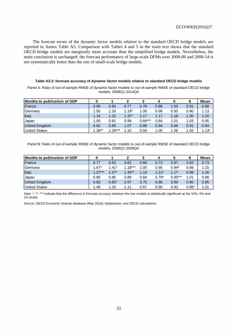
ECO/WKP(2016)37

33

The forecast errors of the dynamic factor models relative to the standard OECD bridge models are

reported in Annex Table A5. Comparison with Tables 4 and 5 in the main text shows that the standard

OECD bridge models are marginally more accurate than the simplified bridge models. Nevertheless, the

main conclusion is unchanged: the forecast performance of large-scale DFMs over 2008-09 and 2008-14 is

not systematically better than the one of small-scale bridge models.

Table A3.3: forecast accuracy of dynamic factor models relative to standard OECD bridge models

Panel A: Ratio of out-of-sample RMSE of dynamic factor models to out-of-sample RMSE of standard OECD bridge models, 2008Q1-2014Q4

Panel B: Ratio of out-of-sample RMSE of dynamic factor models to out-of-sample RMSE of standard OECD bridge models, 2008Q1-2009Q4




France 0.99 0.83 0.77 0.78 0.88 1.00 0.91 0.88

Germany 1.55 1.33 1.19* 1.00 0.98 0.93 0.90 1.13

Italy 1.16 1.32 1.37* 1.17 1.17 1.18 1.00 1.20

Japan 1.00 0.91 0.99 0.84*** 0.84 1.01 1.03 0.95

United Kingdom 0.92 0.89 1.07 0.88 0.94 0.99 0.91 0.94

United States 1.38** 1.29*** 1.15 0.94 1.05 1.06 1.02 1.13*


France 0.77 0.63 0.62 0.66 0.73 0.87 0.82 0.73

Germany 1.67* 1.41* 1.18*** 1.00 0.95 0.94* 0.89 1.15

Italy 1.27*** 1.57* 1.45** 1.18 1.21* 1.17 0.98 1.26

Japan 0.86 0.85 0.89 0.84 0.79* 0.95*** 1.01 0.88

United Kingdom 0.83 0.82* 0.97 0.75 0.86 0.89 0.80 0.85

United States 1.45 1.20 1.11 0.67 0.90 0.93 0.85* 1.01

ECO/WKP(2016)37

34

ANNEX 4. DECOMPOSITION OF FORECAST REVISIONS INTO CONTRIBUTIONS FROM

MODEL PARAMETERS AND CONTRIBUTIONS FROM INDICATORS

The contribution of the re-estimation of model parameters to forecast revisions by the bridge models

can be obtained by computing the difference between two sets of out-of-sample forecasts: one re-

estimating the parameters of the monthly VAR and quarterly bridge equation each month and the other

fixing the parameters at their initial values computed 6 months ahead of the GDP release. This

decomposition method can be formalised using equation (2) and some additional notation:

�̂�𝑡|11 : GDP growth at t, forecast based on information available at date 1 and parameters estimated at date 1



Using similar notations for the monthly indicators and the parameters, equation (2) implies:

�̂�𝑡|11 = 𝑐 +∑𝜙𝑙

1

𝐿

𝑙=1

�̂�𝑡−𝑙|11 +∑∑𝛽𝑖𝑗

1𝑥𝑖,𝑡−𝑗|1𝑄,1

𝐽

𝑗=𝑜

𝐼

𝑖=1

�̂�𝑡|21 = 𝑐 +∑𝜙𝑙

1

𝐿

𝑙=1

�̂�𝑡−𝑙|21 +∑∑𝛽𝑖𝑗


𝐽

𝑗=𝑜

𝐼

𝑖=1

�̂�𝑡|22 = 𝑐 +∑𝜙𝑙

2

𝐿

𝑙=1

�̂�𝑡−𝑙|22 +∑∑𝛽𝑖𝑗


𝐽

𝑗=𝑜

𝐼

𝑖=1

Hence, the forecast revision �̂�𝑡|22 − �̂�𝑡|1

1 can be written as follows:

�̂�𝑡|22 − �̂�𝑡|1

1 = (�̂�𝑡|22 − �̂�𝑡|2

1 ) + (�̂�𝑡|21 − �̂�𝑡|1

1 )

�̂�𝑡|22 − �̂�𝑡|1

1 = (�̂�𝑡|22 − �̂�𝑡|2

1 )⏟ Contribution of parameter changes

+∑𝜙𝑙1(�̂�𝑡−𝑙|2

1 − �̂�𝑡−𝑙|11 )

𝐿

𝑙=1

+∑∑𝛽𝑖𝑗1 (𝑥𝑖,𝑡−𝑗|2

𝑄,1 − 𝑥𝑖,𝑡−𝑗|1𝑄,1 )

𝐽

𝑗=𝑜

𝐼

𝑖=1⏟ Contribution of indicators and past GDP growth rates

Note that the terms (�̂�𝑡−𝑙|21 − �̂�𝑡−𝑙|1

1 ) and (𝑥𝑖,𝑡−𝑗|2𝑄,1 − 𝑥𝑖,𝑡−𝑗|1

𝑄,1 ) may correspond to forecast revisions when

𝑦𝑡−𝑙 and 𝑥𝑖,𝑡−𝑗𝑄

are unknown at dates 1 and 2, or to the effect of the release of GDP or a monthly indicator

at date 2.

ECO/WKP(2016)37

35

This decomposition is actually very similar to the one that is computed in the case of DFM forecasts.

In this case, the forecast revision �̂�𝑡|22 − �̂�𝑡|1

1 can be written as follows, based on equation (3):

�̂�𝑡|22 − �̂�𝑡|1

1 = (�̂�𝑡|22 − �̂�𝑡|2

1 )⏟ Contribution of parameter changes

+∑𝜑𝑙1(�̂�𝑡−𝑙|2

1 − �̂�𝑡−𝑙|11 )

𝐿

𝑙=1

+∑𝛾𝑖1 (𝑓𝑖,𝑡|2

𝑄,1− 𝑓𝑖,𝑡|1

𝑄,1)

𝑟

𝑖=1⏟ Contribution of factor estimates and past GDP growth rates

The only additional step required when using dynamic factor models is to decompose revisions in

factor estimates (𝑓𝑖,𝑡|2𝑄,1− 𝑓𝑖,𝑡|1

𝑄,1) into contributions of news to monthly indicators, which can be done

following the same methodology as Banbura and Modugno (2014). In a nutshell, contributions of

parameter changes to forecast revisions using bridge or dynamic factor models can be meaningfully

compared when they are computed as above.

unclassified eco/wkp(2016)37 - oecd.org · unclassified eco/wkp(2016)37 organisation de...

Documents