unclastfifo 9urt-cl-79-235o 'ieee- -e~m.. · a0-a092 198 .ir force inst of tech...
TRANSCRIPT

A0-A092 198 .IR FORCE INST OF TECH WRIGHT-PATTERSON APR OH F/s q/.FFFICIENdT COOING OF THE PREDICTION RESIDUAL. CU)nEC 79 L L SURGE
UNCLAS"TFIFO 9UrT-Cl-79-235O N
"'IEEE.....-
-E~m..

U-0
1 AINJ1111 RIt 01 0V IK*V"

LEIEL~ cVEFFICIENT CODING OF THE PREDICTION RESIDUAL
L By
LEGND L. BURGE, JR. LECT{: -i ~Bachelor of Science O 8I:
Oklahoma State University
Stll water, Oklahoma, ]1 9 7 2
Master of ScienceOklahoma State University
Stillwater, Oklahoma1973
Submitted to the Faculty of the Graduate Collegeof the Oklahoma State University
*~ in partial fulfillment of the requirementsfor the Degree of
DOCTOR OF PHILOSOPHYDecember, 1979
DIST W UT I N STAApp WvdOP~
D~lbtm UNS".

k 0ti t AI It AT ION t1 1 ilb P~ACF (Whon lpc.I .9.l
REPORT DOCUMENTATION PAGE KId.1Mil ISI-AJ ThNs1-kI R1 P~ONT RUMUL H GOVT ACCESSION NO. 3 RECIPIENT'$ CATALOG NUMbER
79-235D __ _Jj 73/ (__ _ _ _ _
5 TYPE OF REPORT & PERIOD COVERED
(- Efficient Coding of the Prediction Resl 'al, f /ISETTO
6 PERFORMING O'AG. REPOR4T NUMBER
7 AUITHOR(.) 0. CONTRACT OR GRANT NUMBER(*)
Capt Legand.Burge, Jr/
9 &~ERFRMIN ORANIATIO NAE AD ADRES 10 PROGRAM ELEMENT. PROJECT. TASKAREA & WORK UNIT NUMBERS
AFlIT N'lLUDEN'l AT: Oklahoma State University
11 CUNlROLLINU UOII NAME AND ADCRLSS _j._REP ~wrAFFT. NI( U 2Dc9MIi'A Oil 415433 f r- I. - AJBER OF PAGES
/o r 200_R40 MNtORWING AOERNCYI4AME A ADDRLSS(Il t~,f hoii&tf1W OMI .) I5. SECURITYCLS.(ftupfl
UNC LASS
-1S.. 6ECLAS51IFiCA-tiON/DO0%NGR~ADINOSCHEDULE
IS. DISTRIBUTION STATEMENT (of ithit; Npori)
APPIUOVELj FOR PUBLIC RELEASE; DISTRIBUTION UNLIMITED
17. DISTRIBUTION STATEMENT (of thle Sbetract entered in Block 20. it different from kePoft)
18. SUPPLEMENTARY NOTES /Ck, "- L
APPROVED FOR PUBLIC RELEASE: LAW AFH 190-17 FREDRlICC. LYNCF.VU@Ilt. AtrDirfector of Public AffairsZSF SEP 1980 Air Force Institute of Technology (ATQ
19. KEY WORDS (Continue an reverse aide it necesary~ and identify by block nubr)gtPtesn FO 53
20l. ABSTRACT (Continue on revere side It ne~cessary and identify by block number)
ATT-ACHEDI
DD 1JAN 71 1473 EDITION OF I NOV 65IS OSSOLETE UNCLASS (
C U R IT Y C L A SSIF IC A T IO N O F T IS PA G E ( W 7 .Q e. ? '~ b5
1
rjI

Name: Legand L. Burge, Jr. Date of Degree: December 27, 1979U A :r Ivca e .
Institution: Oklahoma State University Location: Stillwater, Oklahoma
Title of Study: EFFICIENT CODING OF THE PREDICTION RESIDUAL
Pages in Study: 200 Candidate for Degree of Doctor of Philosophy
Major Field: Electrical Engineering
Scope and Method of Study: \This thesis presents an efficient method ofcoding the prediction residual using the technique of sub-band cod-ing designed at the bit rate of 9600 bits/second. The energy of theprediction residual is used to distribute the bit allocation by sub-bands such that the perceptual criteria is preserved. The percep-tion is enhanced by transitional information within the phonemeconnections of speech by a technique that weights the energy basedon a normalization factor. A three-tier phoneme classificationis derived from an energy study of the phonemes for the predictionresidual. With this it is shown that speech intelligibility is en-hanced in the coding scheme. The prediction residual is comparedwith the glottal waveform. In association with these results, a newtechnique for pitch extraction is presented using the prediction asthe input signal to calculate pitch. An adequate indication ofcoder quality is described using various types of signal-to-noiseratios.,
Findings and Conclusions: The study of the energy in the predictionresidual of the phonemes shows that the prediction residual is asuitable excitation function rather than the conventional two-sourcemodel. It is shown that the energy of the prediction residual dividesthe phonemes into classes by phonemic aggregations, namely highenergy, low energy and noise groups. The high energy group includesthe vowels and dipthongs. The plosive, fricative and unvoiced pho-nemes compose the noise group. The low energy group is representedby the glides and nasals. The bit allocations scheme discussed inthis thesis is based on this idea and is shown to enhance the per-ceptual aspects of the decoded signal. The normalization factorintroducted further enhances this quality. The sub-band coder isdesigned to exhibit good performance in terms of signal-to-noiseratios for objective measure of quality. The signal-to-noise ratiois only an indication for quantizer performance and generally mustbe supplemented by subjective and perceptual measurements for speechcoding and further work is necessary in this direction.
ADVISER'S APPROVAL______________________________

EFFICIENT CODING OF THE PREDICTION RESIDUAL
BY C Ce A c e ssi on or
LEGAND L. BURGE, JR. -Is'GFI &'
Bachelor of Science LD3 TAB'
Oklahoma State University J, " .o_ .etStillwater, Oklahoma Just__
1972 'By
Master of Science Di.tributicr/Oklahoma State University IStillwater, Oklahoma --tva i>] : 17 J eCoe s
1973 Avail and/orDist. spec al
Submitted to the Faculty of the Graduate Collegeof the Oklahoma State University
in partial fulfillment of the requirementsfor the Degree of
DOCTOR OF PHILOSOPHYDecember, 1979
-,-, -I''; " A " ''
Name: Legand L. Burge, Jr. Date of Degree: December 27, 1979
Institution: Oklahoma State University Location: Stillwater, Oklahoma
Title of Study: EFFICIENT CODING OF THE PREDICTION RESIDUAL
Pages in Study: 200 Candidate for Degree of Doctor of Philosophy
Major Field: Electrical Engineering
Scope and Method of Study: This thesis presents an efficient method ofcoding the prediction residual using the technique of sub-band cod-ing designed at the bit rate of 9600 bits/second. The energy of theprediction residual is used to distribute the bit allocation by sub-bands such that the perceptual criteria is preserved. The percep-tion is enhanced by transitional information within the phonemeconnections of speech by a technique that weights the energy basedon a normalization factor. A three-tier phoneme classification isis derived from an energy study of the phonemes for the predictionresidual. With this it is shown that speech intelligibility is en-hanced in the coding scheme. The prediction residual is comparedwith the glottal waveform. In association with these results, a newtechnique for pitch extraction is presented using the predictionresidual as the input signal to calculate pitch. An adequate indi-cation of coder quality is described using various types of signal-to-noise ratios.
Findings and Conclusions: The study of the energy in the predictionresidual of the phonemes shows that the prediction residual is asuitable excitation function rather than the conventional two-sourcemodel. It is shown that the energy of the prediction residual dividesthe phonemes into classes by phonemic aggregations, namely highenergy, low energy and noise groups. The high energy group includesthe vowels and dipthongs. The plosive, fricative and unvoiced pho-nemes compose the noise group. The low energy group is representedby the glides and nasals. The bit allocations scheme discussed inthis thesis is based on this idea and is shown to enhance the per-ceptual aspects of the decoded signal. The normalization factorintroducted further enhances this quality. The sub-band coder isdesigned to exhibit good performance in terms of signal-to-noiseratios for objective measure of quality. The signal-to-noise ratiois only an indication for quantizer performance and generally mustbe supplemented by subjective and perceptual measurements for speechcoding and further work is necessary in this direction.
ADVISER'S APPROVAL
, .1..

EFFICIENT CODING OF THE PREDICTION RESIDUAL
Thesis Approved:
. Deanof the Graduate Colleg&

ACKNOWLEDGMENTS
I extend my sincere thanks and gratitude to Dr. Rao Yarlagadda, my
thesis adviser and chairman of my doctoral committee, for his dedication
and guidance during the term of my graduate program. His interest and
encouragement through understanding has contributed significantly to
realize the completion of this dissertation. My appreciation is due to
Drs. Bennett Basore, Craig S. Sims, and Ronald D. Schaefer, my committee
members, for their helpful comments and generous contribution of time
throughout this research.
I owe special recognition to Dr. Cheryl Scott for stimulating dis-
cussions concerning aspects of speech science.
A special thanks is due to Drs. Charles Bacon, H. Jack Allison and
Robert Mulholland for stimulating discussions and encouragement during
this work. A sincere appreciation to Dr. Lynn R. Ebbesen and John
Perrault for their assistance and accessibility of computer time.
I would like to thank the United States Air Force for providing me
the opportunity to complete my degree through the AFIT Civilian Institu-
tions Program. I am grateful to Lt. Col. John Kitch, Jr., and Capt.
Samuel Brown, Jr., for their understanding and helpfulness during my
academic tenure.
I am grateful to the Defense Communications Engineering Center (OCA)
in Reston, Virginia, for their support during the term of the research.
The stimulating discussions and kindness awarded me by Mr. Gerald Helm
iii

and Mr. George Moran is appreciated. The assistance of Mr. William Mills
and Ms. Elaine Bernd was greatly appreciated during the term.
My sincere gratitude to Ms. Debbie Perrault and Ms. Louise Sumpter
for their excellent typing of this dissertation. I would like to ack-
nowledge Mr. Eldon Hardy for the excellent drawing of the figures.
I owe special thanks to Mr. Legand L. Burge, Sr., Mrs. Bobbie J.
Burge, Mr. Richard Jones, Mrs. Wilba Jones, Mrs. Annie Dean, Rev. Dr. and
Mrs. Joe Edwards, Rev. and Mrs. Richard Thompson, Mr. and Mrs. Glenn
Mosely, Mr. Lynn R. Osborn, Mr. Lew Phillips, and Mr. Raymond A. Young
for their encouragement throughout this work.
The cooperation, patience and understanding of my wife, Claudette,
has been greatly appreciated. My son and daughter, Legand and LeAnn, are
acknowledged for the continued source of motivation for which this effort
was begun.
iv

TABLE OF CONTENTS
Chapter Page
I. INTRODUCTION ...... .. ........................ I
1.1 Statement of the Problem ..... ............. 11.2 Review of the Literature ..... ............. 81.3 Organization of the Thesis .... ............ 20
II. PREDICTION RESIDUAL AND THE PITCH EXTRACTION ... ........ 22
2.1 Introduction ....... ................... 222.2 Mechanism of Speech Production .... .......... 242.3 Model of the Vocal Tract ..... ............. 342.4 A Parallel Between Glottal Waveform and the
Residual Signal .... ................ ... 352.5 Review of Linear Prediction Analysis ... ....... 392.6 Short-Time Analysis ...... ............... 482.7 Implementation of Operations for the Calculation
of the Prediction Residual .... ........... 532.8 A Novel Approach to Pitch Extraction ... ....... 54
2.8.1 Types of Problems Associated withPitch Extraction ... ............ ... 54
2.8.2 Advantages and Disadvantages for Usingthe Prediction Residual as a Sourcefor Pitch Extraction .... .......... 58
2.8.3 A Novel Pitch Extractor ............ ... 612.8.4 Pitch Extraction Results .... ......... 63
2.9 Summary ...... .. ..................... 67
III. SUB-BAND CODING OF THE PREDICTION RESIDUAL ........... ... 68
3.1 Introduction ....... ................... 683.2 Coding Methods ....... .................. 693.3 Transform Coding .... ................. ... 763.4 Sub-Band Coding ...... ................. 80
3.4.1 Sub-Band Coding and Transform Coding . . 853.5 Determination of Frequency Sub-Bands Based on
Articulation Index ..... ............... 863.6 Transitional Information ..... ............. 943.7 Relation of Perception to Intelligible Speech 973.8 Basis for Coding the Prediction Residual ....... 99
3.8.1 Energy Distribution .............. ... 1013.9 Summary ...... .. .................... 110
v

Chapter Page
IV. ENERGY BASED SUB-BAND CODING ALGORITHM ............. ... 11
4.1 Introduction ...... ................... 114.2 Bit Allocation ......................... 1124.3 Sub-Band Encoding of the Prediction Residual . . 1204.4 Adaptive Uniform Quantization .... .......... 1314.5 Signal-to-Noise Ratio Performance Measurements 1354.6 Computation for Coding the Prediction Residual 1384.7 Summary ..... .. ..................... 141
V. SUMMARY AND SUGGESTIONS FOR FURTHER STUDY .......... ... 143
5.1 Summary ..................... 1435.2 Suggestions for Further Study. .......... 146
5.2.1 PARCOR Coefficient Study of Sensitivity 1465.2.2 Sub-Band Coding Using Subjective
Measurements ............... 1465.2.3 Energy Threshold Matrix Study. ....... 1465.2.4 Integer-Band Coding of the Prediction
Residual .. ................ 1475.2.5 Prediction Residual and Noise ... ....... 1475.2.6 Modeling the Prediction Residual .. ..... 148
BIBLIOGRAPHY ...... ... ........................... 149
APPENDIXES
APPENDIX A - DEFINITIONS RELATED TO SPEECH SCIENCE 161
APPENDIX B - COMPUTER PROGRAMS FOR CODING THEPREDICTION RESIDUAL .... ........... 165
APPENDIX C - ARTICULATION INDEX .............. ... 189
APPENDIX D - SONAGRAMS ...... ................ 194
vi

LIST OF TABLES
Table Page
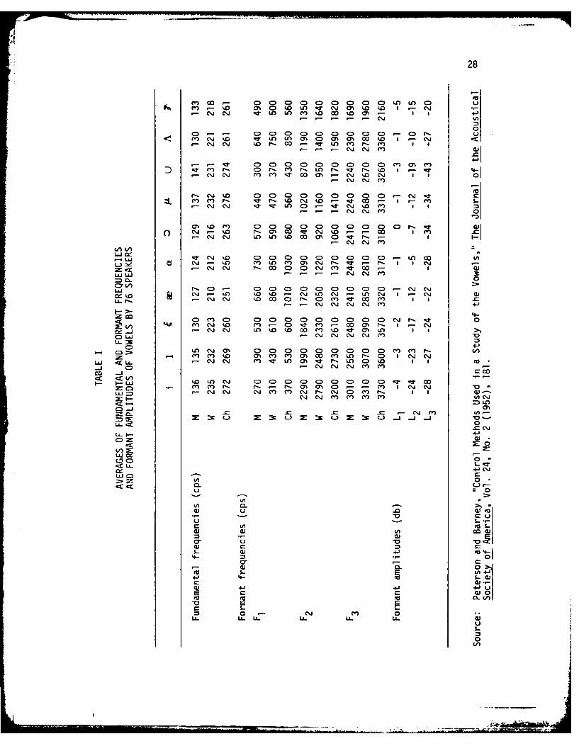
I. Average of Fundamental and Formant Frequencies and FormantAmplitudes of Vowels by 76 Speakers .. ........... ... 28
II. Representation of IPA Phonemes with Examples ... ........ 30
III. Comparison of Fundamental Frequencies .. ........... ... 66
IV. Sub-Band Partitioning Example ... ............... .. 81
V. Adjustments to the Spectrum of the Speech Signal ........ 88
VI. Adjustments for Noise Spectrum ..... ............... 89
VII. Frequencies Related to One-Third-Octave-Bank Method .... 91
VIII. Frequencies Related to Octave Method .... ............ 92
IX. Sentence Data ..... ... ....................... 102
X. Phonemic Data ..... ... ....................... 103
XI. Energy by Phoneme for the Predictive Residual ... ....... 105
XII. Phoneme Energy Groupings .... .................. .107
XIII. Symbolic Representation of Energy Distribution ......... 108
XIV. Energy Threshold Matrix ...... .................. 109
XV. Symbolic Representation of Bit Distribution .. ........ 113
XVI. A Priori Bit Matrix Distribution ... .............. .116
XVII. Sub-Band Coder Cutoff Frequencies .... ............. 122
XVIII. Integer-Band Sampling Cutoff Frequencies for 8000 HertzSampling Rate ..... ... ...................... 125
XIX. Sub-Band Coder Parameters Relative to High Energy Phonemes . 126
XX. Sub-Band Coder Parameters Relative to Low Energy Phonemes 127
vii

Table Page
XXI. Sub-Band Coder Parameters Relative to Noise EnergyPhonemes. .. .. .. ... .. ... .. ... .. .....128
XXII. Representation of Samples for a Frame for High Energy ... 12Sound......... .... .. .. .. .. .. ....... 2
XXIII. Signal-to-Noise Performance Measurement for SeveralPhonemes. .. .. .. ... .. ... .. ... .. .....137
XXIV. Data Blocks for Processing and Storage .. .. . .. ..... 138
XXV. Frequency Bands of Equal Contribution to Articulation Index 192
viii

LIST OF FIGURES
Figure Page
1. Model of Speech Production as the Response of a Quasi-Stationary Linear System ..... .. .................. 3
2. Block Diagram of LPC Analysis ...... ................. 5
3. Prediction Residual Formed by Speech Through an InverseFilter ..... .... ........................... 23
4. Cross-Sectional View of the Human Vocal Tract System .. ..... 26
5. Distinctive Feature of the Phonemes of English Indicating thePresence or Absence of a Feature ... .............. ... 33
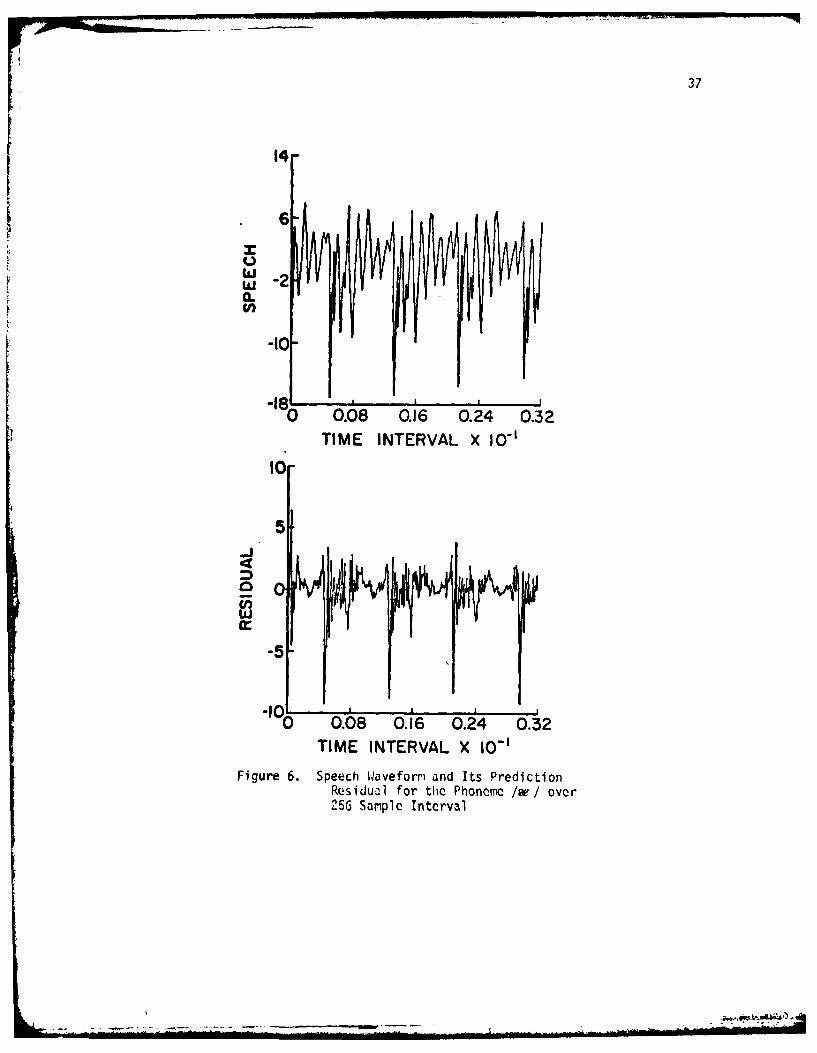
6. Speech Waveform and Its Prediction Residual for the Phoneme/w/ over 256 Sample Interval ...... ................ 37
7. Spectrum of Residual Signal for the Phoneme /ae/ . ....... ... 38
8. Implementation for Generation of Forward and BackwardPrediction Errors ..... ...................... ... 41
9. Detailed Structure of PARCOR Implementation for jth Stage . . . 49
10. Analysis and Synthesis Models for Lattice Structure ........ 50
11. Sequence of Operations Related to Calculation of thePrediction Residual, r(n) ...... .................. 55
12. Two Methods of Determining Pitch Period .............. ... 57
13. Prediction Residual Waveform for Phoneme 1w/ over 256Sample Segment ...... ....................... .. 60
14. Block Diagram of Pitch Extraction Method .... ........... 64
15. Basic Component of Channel Vocoder ... .............. ... 71
16. Block Diagram of Channel Vocoder Analyzer ............. .. 72
17. Block Diagram of Channel Vocoder Synthesizer .......... ... 73
18. LPC Vocoder ...... ... .......................... 74
ix

Figure Page
19. Block Diagram of the Implementation of Transform Coding . . . 77
20 Partitioning of Frequency Spectrum into Four Sub-Bands .... 83
21. Sequence of Operations Relating to the nth Sub-Band ........ 84
22. Relation Between AI and Various Measures of SpeechIntelligibility ....... ....................... 93
23. Transitional Cueing for Consonant-Vowel for Phonemes /a/and /d/ ....... ........................... . 96
24. Normalized Energy Distribution by Sub-Band ... .......... 106
25. Power Density of Speech Signal ..... ................ 115
26. Distribution of the Normalization Factor .... ........... 118
27. Flow Chart for Bit Allocation ... ................. .. 119
28. Bit Distribution for Sub-Bands by Energy Bands ... ........ 121
29. Bit Distribution for Phonemes by Frame .. ............ ... 123
30. Characteristic of the Adaptive Uniform Quantizer ... ....... 133
31. Flow Chart for Coding Residual Signal .... ............. 139
32. Composite Articulation Index vs. Cutoff Frequencies ofIdeal Lowpass Filters ....... .................... 191
x. - -

LIST OF SYMBOLS
M - Total number of data points
sn - Signal
ai - Forward lattice LPC filter coefficients
bi - Backward lattice LPC filter coefficients
R(k) - Residual signal k = 0, 1, ..., M-1
p - Order of the LPC filter
F1, F2, ... - Formant frequencies
r,(m) - Output of the ith bandpass filter
m = 0, 1, ..., M-l; z = 1, 2, ..., B
re (k) - Decimated signal r(k)
t - Bandpass filters are assumed to be contiguous;
i gives the lowest frequency corresponding to
the xth bandpass filter
h n(k) - Impulse response of nth lowpass filter
associated with the nth sub-band
Wt - Bandwidth of the ith bandpass filter
Wn - Edges of the bandpass filter
en (k) - Modulated signal of sub-band
N, N. - Samples available per frame1
fa - Fundamental frequency
fl9 f29 ... - Harmonics of the fundamental
f S- Original sampling frequency
f . - Sampling frequency for the ith sub-band
xi L

g(t), G(w) - Represents glottis excitation function in the
time and frequency domains
V(t), V(w) - Represents vocal tract filter in the time and
frequency domains
s(t), S() - Represents speech waveform in time and fre-
quency domains
x(n), y(n), x(k), y(k) - Speech sample sequency
xf(n) - Forward prediction of x(n)
xb(n) - Backward prediction of x(n)
ef(m) - Forward prediction error or prediction resid-
ual signal
efn (k) - Output of the nth bandpass filter
eb(k) - Backward prediction error
R. - Autocorrelation of x(n)
E. - Residual signal at the jth stage
C. - Cross correlation between forward and backward
prediction errors
kj+ I - Partial correlation coefficients (PARCOR) of
(j+l)st stage
A p(Z) - Transfer function between forward prediction
error and speech sequence for pth stage
B p(Z) - Transfer function between backward prediction
error and speech sequence for pth stage
rj+ l - Reflection coefficient of (j+l)st stage
o2 - Variance of speech source
y - Transform coding coefficients
A - n x n matrix
xli

I
D - Mean-square overall distortion
J. - Number of bits/sample
6 - Correction factor for a quantizer
- Average bit rate
Rxx, Ry - Covariance matrices for x and y
A i - Eigenvalue of Rxx
k.. - Bits/sample corresponding to the ith energy
and jth frequency band
Efn(k) - Discrete Fourier transform coefficient
E - Energy of the nth sub-band
E. i- Energy of the signal for the ith energy band
and jth frequency band
ET.. - Energy threshold for the ith energy band and
jth frequency band
kA. - A priori bits/sample corresponding to the ith
energy band and jth frequency band
a. - Normalization factor1
- Discrete Cosine Transform coefficientn
A - Quantizer step size
- Quantizer array
Q - Quantization value array
- Quantizer level
xiii _ ,

CHAPTER I
INTRODUCTION
1.1 Statement of the Problem
The structural unit of speech composition is the speech sound called
the phoneme. Its variations are called allophones. It can be said also
that phonemes relate to the linguistic basis of a language. However,
phonemes are not "bricks," i.e., the human has been endowed with the
ability to communicate in a continuous mode. Because we speak in an
uninterrupted fashion in order to complete our thoughts, the phonemic
structure connects itself by transitional cues for the perception of cer-
tain phonemes [1]. It is this transitional information that is needed
for absolute discrimination of speech and speech-like sounds [2]. It is
the transitional information that is needed for efficient excitation of
a speech synthesizer.
To synthesize intelligible speech, the perceptual aspects of speech
sounds have to be used. In other words, the ability for humans to dis-
criminate and differentiate a speech sound with their over-learned senses
must be incorporated into the speech synthesis technique. The speech
synthesis must include perceptual enhancement, and the inclusion of
transitional information (that is, frequency shifts). Transitional
information is the loci of frequency determined by the place of
tSome of the words related to the science of the speech waveform are
defined in APPENDIX A.
I II lli " lll ' F~1

2
articulation that connects the phonemes. Phonemes are the basic speech
sound element used to make a word. One can also say that a phoneme is an
idealized structural unit of language which serves to keep words apart.
It is an astonishing fact as to how the human brain stores rules to keep
track to one's language for communicating. The object of speech synthe-
sis is to come as close as possible to this occurrence.
The history of synthetic voice coding had its origination with H. W.
Dudly in 1939 [3] [4]. The Dudley speech reproduction model consists of
a filter representing the vocal tract resonance characteristics driven by
an artificially synthesized excitation signal. The filter and the excita-
tion signal parameters are updated periodically. To determine the filter
characteristics, Dudley used the Fourier spectrum of the speech as a
basis. The excitation signal cansists of a pulse train for voiced sounds
and random noise for unvoiced sounds. The model that Dudley has repre-
sented is essentially the basis of many methods today [5] [6] [7]. Some
of these ideas are discussed below.
A basic model of the speech waveform is to assume a linear quasi
time-invariant system which responds to a periodic or noiselike excita-
tion. This linear time invariant system represents the vocal tract. If
the vocal tract is assumed to be fixed, then the output of the system is
a convolution between the excitation and vocal tract transfer function
(see Figure 1).
Recently considerable interest has been given to methods of digital
analysis and synthesis of speech assuming the presented model. A method
that has proven to be efficient for encoding the speechwave is linear
prediction [6]. The linear predictive encoder was developed to improve
the channel vocoder voice quality and intelligibility [7]. The difference

4- L
to
-0 ,. -
4..j
*00 fa
00
4J0 41
_ ~00
0
4- L. a
0 c.
04

4
between the linear predictive coded (LPC) vocoder and the channel vocoder
is the filter. There are two types of LPC vocoders, a pitch-excited and
a residual-excited. The difference between the two is how the excitation
signal is characterized for the synthesis filter. In the pitch-excited
LPC vocoder, the model of the vocal tract, with glottal flow and radia-
tion, is represented by the predictor coefficients. These coefficients
are transmitted together with the information regarding the excitation of
the speech, i.e., pitch, voiced/unvoiced decision and the gain. Much
research has been done toward the pitch-excited LPC vocoder. Two methods
have been discovered, the autocorrelation [8] [9] and the covariance [6]
methods. The residual-excited methods can be characterized the same way.
However, instead of using pitch, voiced/unvoiced desicion and gain, the
residual is encoded and transmitted. The residual is the difference be-
tween the actual and predicted speech signals. This technique also car-
ries the name adaptive predictive coding (APC). The channel vocoder, on
the other hand, uses a set of narrowband filters whereas the linear pre-
dictor uses an all pole digital filter. The linear predictive filter
describes the frequency response of the vocal tract system by the pre-
dictor coefficients. Its function is to decompose the speech into two
waveforms. One waveform represents the parameters that are time-varying
such as predictor coefficients, partial correlation coefficients and
other parameters that represent the formant frequency characteristics.
The other waveform is the prediction residual. Figure 2 describes a
block diagram of the LPC analysis.
The prediction residual is the ideal signal for an excitation func-
tion for the linear predictive analysis and synthesis model because it
contains the actual information instead of the pseudo-model, a pulse

5
1211
11)5
C,z
w(0 -
0~411) -~
0
E
U
0
Ca
044 C\J
aJ
S.-
Li~IL0.-J
Uwa.11)

6
train or random noise [10]. In addition, phasing information is embedded
in the prediction residual. Furthermore, since the analysis filter is
the inverse of the synthesis filter, the decomposed waveform can be re-
constructed to form the input speech waveform by updating the parameters
[7] [11]. The prediction residual also follows the actual speech excita-
tion model g(t) in Figure 1 [12]. The function, g(t), represents the
glottal pulse which is also called the glottal volume velocity at the
vocal cords or glottis. In order to ideally model the voice reproduction
system, it is necessary to use a system whose properties are similar
acoustically to the glottis and vocal tract. It is best to model the
excitation signal with an analogous function to the glottis waveform for
input to the vocal tract. It is well known that for nonnasal voiced
speech sounds, the transfer functions have no zeros [5]. For these par-
ticular sounds, the vocal tract filters can be approximated by an all
pole filter. It is also known that the shape and periodicity of the
glottis excitation are subject to large variations [12]. However, with
the linear predictive model the features of the glottal flow, the vocal
tract, and the radiation, which is the output from the mouth, are included
into a single recursive filter. To separate the glottal flow from the
vocal tract involves a deconvolution. Some authors have avoided this sep-
aration of the source function; however, the artificial excitation used by
them represents only a good approximation to the prediction residual for
unvoiced sounds. Moreover, for voiced sounds, the artificial excitation
could be improved. The prediction residual should be used for the excita-
tion function, because it contains the following characteristics:
1. It is repetitive at the pitch frequency.
2. It has basically a flat amplitude spectrum; however, it includes

7
details that relate to the suprasegmentals of the individual and of the
spoken words.
3. It includes the noisiness of opening and closing of the glottal
mechanism indicating phase information.
4. It includes the fact that voiced fricatives and stops are a com-
bination of noise and a repetitive signal.
Noting the speech characteristics in the residual signal, several
authors have investigated the coding aspects of the prediction residual
[13-32]. However, the speech intelligibility aspects, such as Articula-
tion Index (Al) [29], have not been used in these. The Articulation Index
concept has been used effectively in the sub-band coding of speech [36].
The sub-band coding, based upon Al, allows for an efficient bit distribu-
tion in coding. This thesis combines all these ideas and presents an
efficient method of coding the prediction residual using the concepts of
sub-band coding. A literature survey related to these areas is presented
in the next section.
One important aspect of coding is bit rate. For certain narrow band
rates, the coding of the prediction residual is not feasible [13]. Also,
it has been shown that 9,600 bits/second is feasible for transmission of
residual and filter parameters, and is practical over voice grade lines
[35]. In the future, lower data rates have to be used for cost effec-
tiveness. At present, rates below 6,000 bits/second yield speech quality
of a synthetic nature. Rates between 6,000 bits/second and 16,000 bits/
second demonstrates good coammunication quality. Studies have shown and
present operating equipment demonstrate that a 16,000 bits/second trans-
mission rate and above yield toll telephone quality. The thrust of the
governmental community for designing voice switch networks has been
1 I

8
recently toward 9,600 bits/second rate. At this rate, the communicators
can comprehend the language spoken; however, there is some drop-off in
speaker recognition but not as drastic as at rates closer to 6,000 bits/
second. With the advent of mircroprocessing systems more sophisticated
algorithms can be implemented with small monetary investments. This
thesis presents the coding and decoding of the residual signal using sub-
band coding at a data rate of 9,600 bits/second.
1.2 Review of the Literature
Predictive systems related to speech have evolved through the years.
A brief survey of these systems is presented below. In earlier studies
of predictive coding systems with applications to speech signals, the
linear predictors were limited to fixed coefficients in an interval [17].
In more recent studies, it was found that since the speech signal has non-
stationary properties, the linear predictor does not efficiently predict
the signal at each interval. In work by Atal and Schroeder [6], an adap-
tive predictive system took into account the quasi-periodicity of speech
signals. In addition to being the classic forerunner for adaptive pre-
dictive coding (APC) of speech signals, this is a more elaborate predictor
than the one with fixed coefficients which is suited for characteristics
of speech sounds. Basically, the residual signal along with the predictor
provides sufficient information for the receiver to regenerate the input.
In this, pitch is determined from the residual signal. Atal and Schroeder
[22] have examined predictive coding of speech signals recently. They
have shown that speech quality can be improved by masking quantizer noise
over the speech signal. Atal and Hanauer [5] described an efficient en-
coding of the speech wave by representing it in terms of time-varying
9
parameters related to a transfer function of the vocal tract and by model-
ing the excitation.
In work by Dunn [13], the linear predictive coded residual signal was
generated by a feed-forward linear predictive coding (LPC) analyzer and
encoded using delta modulation (DM). The signal was transmitted at a bit
rate of 9,600 bits/second. Gibson, Jones, and Melsa [14] have introduced
a method called sequential adaptive prediction which utilized differential
pulse code modulation (DPCM) with an adaptive quantizer and an adaptive
predictor using Kalman filtering. This work was improved upon by Cohn and
Melsa [15] using adaptive differential pulse code modulation (ADPCM) for
encoding the prediction residual. A method using the Kalman filter for
the adaptive predictive encoder was introduced by Goldberg and others
[16]. This system was real time APC that was implemented on a minicompu-
ter. An adaptive residual coding using an adaptive predictor, adaptive
quantizer, and a variable length coder was studied by Qureshi and Forney
[18]. In these studies, a class of speech digitization algorithms is
described for use at bit rates of 9,600 to 16,000 bits/second. These sys-
tems involve an adaptive predictor, an adaptive quantizer, and a variable
length coder. This is a practical version of a residual encoder previous-
ly studied by Melsa and others [14]. Most recently, the method of vari-
able length coding of the prediction residual was studied by Berouti and
Makhoul [19]. This system of APC uses a noise spectral shaping filter to
solve the granular noise quantization problem and an indefinite quantizer
to solve the overload quantizing problem.
A voice-excited predictive coder (VEPC) by Esteban and others [20]
uses a baseband excitation of the residual and splitband coding by signal
decimation/interpolation. Furthermore, quadrature mirror filters are
10
implemented in order that the aliasing properties could be taken advan-
tage of in the synthesizer.
The most recent work by Cohn and Melsa [21] [23] involves the imple-
mentation of a speech coding algorithm for digital transmission of speech
at 9,600 bits/second using a sequential, adaptive linear predictive coder,
an adaptive source coder, and multipath tree-searching algorithm to gen-
erate quality speech. This is an extension of the previous work done on
a residual encoder which was an improved ADPCM system for speech digiti-
zation. Chang [24] has extended this work and incorporated a noise re-
sistant code for transmission.
In work by Magill and others [25], a feed-forward LPC analyzer was
used with an encoding method of Adaptive Delta Modulation (ADM) and an
experimental method of encoding the residual by DPCM. This is referred
to as a residual excited linear predictive (RELP) vocoder. It combines
the advantages of linear predictive coding and voice-excited vocoding.
Recently, Dankberg and Wong [26] have implemented a new version of
the RELP vocoder. Their results have included a development of a pitch
predicted ADPCM residual encoder and a harmonic generator. Viswanathan
and others [27] considered the use of voice-excited linear predictive
(VELP) and RELP coders for speech. They have studied in detail the var-
ious aspects of these coders and have attempted to maximize speech qual-
ity as a result. They also studied the advantages and disadvantages of
baseband residual transiission and baseband speech transmission.
In recent work, Kang [28] studied the development of a narrowband
voice digitizer that improves speech quality, intelligibility and relia-
bility. The principle of LPC is used in implementing the lattice filter
for the analysis and synthesis. Itakura and Saito [9] [30] have used
.......

the lattice method for LPC analysis of speech. The thrust has been for
improved quantization of partial correlation (PARCOR) coefficients.
Makhoul [31] has presented a class of stable and efficient lattice meth-
ods for linear prediction of speech. In this, an indepth study is made
on PARCOR coefficients. If the all pole function is stable, then the
lattice obtained from this is stable; furthermore, since the PARCOR co-
efficients are bounded, stability is guaranteed and an efficient quanti-
zation method can be used.
In work by Flanagan [32], it is shown that the residual approximates
the glottal waveform. In any excitation system, the closer one can
approximate the physical model, the better response one gets from the
system. Flanagan's work enhances this concept to use the residual wave-
form as the excitation to the speech synthesizer.
Rabiner and others [33] have studied the LPC error signal. The work
investigated the variation of the prediction error as a function of posi-
tion in an analysis frame within a single stationary speech segment. The
error signal has the frequency range of the actual speech.
The work of Goodman [34] found the analog signal can be divided into
several nonoverlapping frequency bands. Each band can be sampled and
quantized independently. The result is an improvement in encoding effi-
ciency over straight sampling and quantizing of signals that are spectrum
peaked. Crochiere and others [36] [37] have applied this to speech sig-
nals in the digital domain. This is referred to as sub-band coding (SBC).
This approach provides a means of controlling and reducing quantization
noise in the coding.
A pilot study of speech waveform coding techniques were studied by
Tribolet and others [38]. The study compared subjective ratings to the

12
various quality (objective) measures for speech waveform coders. Tribo-
let and others examined four different speech waveform coder algorithms
for low-bit rate applications, and studied these relationships for over-
all objective and subjective ratings for quality. The algorithms were:
adaptive differential PCM with a fixed predictor (ADPCM-F), sub-band cod-
ing (SBC), ADPCM with a variable predictor (ADPCM-V) and adaptive trans-
form coding (ATC). The transmission rates studied were 24,000, 16,000,
and 9,600 bits/second. The objective measures used were a conventional
signal-to-noise ratio, frequency weighted signal-to-noise ratio, log
likelihood ratio, and an articulatory bandwidth measure. The results of
the study were that if complexity/cost was of no concern, then ATC is the
most attractive of the group coders. However, if complexity/cost was a
concern, then SBC is an attractive choice. ADPCM-F had the poorest qual-
ity for its complexity; ADPCM-V was the most costly for its quality. The
transform coding and the sub-band coding will be explained in detail in
Chapter II.
In the work by Barabell and Crochiere [39] a new design of the sub-
band coding has been implemented for low-bit rate coding of speech. This
study applied quadrature filters to SBC. This method has also employed
pitch prediction within the sub-bands. Crochiere [40] has implemented a
novel approach for pitch extraction in the SBC. The method uses digital
linear phase shifters based on a bandpass interpolation scheme to achieve
the non-integer delays necessary in the feedback loop for the pitch pre-
dictors. It uses the fractional sample delay in the pitch loop and per-
mits the processing of the pitch prediction in each sub-band to be
performed at the sub-band sampling rate which contributes to the effi-
ciency of the algorithm.
,.__ _~~~~~~~~~~~ ~.. ........ .... . . . .. . .. .I l -,, - , b

13
Pitch detection algorithms that have been mentioned above have one
basic goal. That is, make a voiced or unvoiced decision and during cer-
tain periods of voiced sounds, estimate the pitch period.
There are three areas of categorization for pitch detectors. First,
there is a group that uses time-domain properties of speech signals.
These pitch detectors operate directly on the speech waveform in order to
estimate the pitch period. The measurements that are usually taken are
minimum and maximum amplitude, zero-crossing and autocorrelation measure-
ments. With these detectors, it is assumed the formant structure has been
minimized by preprocessing the speech. A second category for pitch detec-
tion algorithms uses frequency-domain properties of speech signals. A
periodic signal in the time-domain will consist of a series of impulses
in the frequency-domain located at the fundamental frequency and its har-
monics. Therefore, one can make measurements in the frequency domain to
determine the pitch period. The final group combines both time and fre-
quency-domain concepts of the speech signals in order to determine pitch
period. This is a technique that is used which flattens the signal with
frequency-domain techniques and subsequently uses autocorrelation mea-
sures to estimate the pitch period. These are called hybrid techniques.
Previous work of the pitch detection algorithms and related works that
have been published will be discussed.
There are several documented pitch extraction methods that have been
published recently. In earlier methods, analysis of the speech time wave-
form were attempted by visual inspection of spectrograms which involved
the manual determination of pitch [41]. At this time the authors noted
the requirement for an automatic scheme of some kind. Pinson [42] used
the method of Mathews, Miller, and David [41] to estimate a time-domain

14
synchronous pitch which in turn was used to determine frequencies and
bandwidths of vowel formants.
Sondhi [43] introduced three methods for finding the pitch period.
The first method spectrum flattens the signal and corrects the phase to
synchronize harmonics. A second method by Sondhi also flattens the spec-
trum but adds an autocorrelation to determine pitch. The third method
center clips the speech signal and uses autocorrelation for determination
of pitch. Using the method by Sondhi, a real-time digital hardware pitch
detector was implemented by Dubnowski, Schafer, and Rabiner [44].
There are also methods that make use of the power spectrum in the
determination of the pitch. One such method is called cepstrum pitch
determination. The cepstrum is defined as the power spectrum of the log-
arithm of the power spectrum, or mathematically expressed, the cepstrum,
Q(T) [45] [46], is
NO = [f logF(w)l2 cos (wT) dw 2 (1.1)0
where f(t) is the speech signal, w is the frequency in radians, and
F(W)= f0f(t) e-jWt dt (1.2)
More recently, using digital inverse filtering techniques, Markel
has innovated a method for estimating the fundamental frequency of voiced
speech using time-domain analysis. This method has been referred to as a
simplified inverse filter tracking (SIFT) algorithm [47]. The pitch per-
iod is estimated by an interpolation of the autocorrelation function in
the neighborhood of the peak of the autocorrelation function.

15
Another recent algorithm that determines the fundamental frequency
of sampled speech is implemented by segmenting the signal into pitch per-
iods. This is done by identifying the beginning of each pitch period.
This algorithm is called the data reduction pitch detector by Miller [48].
To obtain the appropriate identity of the beginning of the pitch period,
the method detects the cycles of the waveform based on intervals between
major zero crossings. The rest of the algorithm determines principal
cycles, which correspond to true pitch periods.
In work presented by Gold [49], it is assumed that pitch extraction
could be obtained by a visual inspection of the speech wave and is the
best obtainable. The computer program contains essentially four sections.
First, a voiced/unvoiced decision is made and the two portions are sepa-
rated. Each voiced portion is labeled as relative maximum, then the peak
detector is compiled. The third decision is to determine the spacing;
this in turn determines which samples will be called pitch peaks. Finally,
a procedure is necessary to eliminate spurious peaks and add into the
speech missing pitch peaks. The program is implemented such that editing
can make the best pitch selection.
The work of Gold and Rabiner [50] using parallel processing for esti-
mating pitch is a modified version of Gold [49]. A series of measurements
are made to find the peaks and valleys of the signals. There are six
cases used to determine this. Each is followed to determine if the sample
will be an impulse or zero. The rules of this are:
1. An impulse equal to the peak of the signal occurs at the point of
each peak in time.
2. An impulse equal to the difference between the signal present
peak and the past peak amplitude occurs at the point of each peak in time.
.. . .... .. .. ... .. .. .. ' " " -... . " ': i i~n , i € ... ... _,,. . .. .. . ..... ., .. . .. _. - - .,,-. .. . .. ...T . . - N

16
3. An impulse equal to the difference between the signal present peak
and the past peak amplitude occurs at the point of each peak in time. (If
the difference is negative, then it is set to zero.)
4. An impulse equal to the negative of the peak of the signal occurs
at each negative peak in time.
5. An impulse equal to the negative of the peak at each negative
peak plus the peak of the preceding negative peak occurs at each negative
peak in time.
6. An impulse equal to the negative of the peak at each negative
peak, plus the negative of the preceding local minimum occurs at each
negative peak. (If this difference is negative, then the impulse is set
to zero.)
From this technique six estimates are formed. These estimates are
combined with the two most recent estimates for each of the six pitch
detectors. The values are then compared within an acceptable tolerance;
the decision is made for the most occurrences. This value is declared
the pitch at that time. An unvoiced decision is made when there is an
inconsistency between the comparisons for the pitch period.
Another method by Atal [51] is based upon LPC. This detector ini-
tializes with a voiced/unvoiced decision. Upon being classified as
voiced, the speech is low-pass filtered and then decimated by five to one.
The method uses a 41-pole LPC analysis on 40 ms seconds of frame data to
generate the speech harmonics. Then, a Newton transformation is used to
spectrally flatten the speech. A peak picker determines the pitch period
at the five to one decimated rating. Then, the signal is interpolated and
a higher resolution is used to obtain the pitch period.

17
The average magnitude difference function (AMDF) pitch extractor
[52] is a variation of autocorrelation analysis to determine the pitch
period of voiced speech sounds. This method takes advantage of the per-
iodicity of voiced speech. It calculates a difference function that at
multiples of the pitch period will dip sharply when the delayed speech
and original speech are compared. The AMDF function is implemented with
subtraction, addition, and absolute value operations, whereas autocorrel-
ation methods use addition and multiplication operations. For this rea-
son, the AMDF function is attractive for real-time operations.
Another real-time pitch extraction method, based on linear predic-
tive techniques, is presented by Maksym [53]. The method employs a non-
stationary error process from the adaptive predictive coder by Atal [5].
The algorithm in addition to pitch period extraction also detects voiced
speech. The basis of the method uses a predictive one-bit quantizer with
an adaptive algorithm for determining prediction coefficients. Since the
method operates on the short-term prediction of the speech waveform, the
presence of the glottal excitation can be detected.
A semiautomatic pitch detector (SAPD) [54] has been presented by
McGonegal, Rabiner, and Rosenberg. This method semiautomatically deter-
mines the pitch contour of an utterance. An autocorrelation of the speech
is generated. The cepstrun of the unfiltered speech is computed. These
displays are shown on a scope on a frame-by-frame basis. The computed
pitch period for each waveform is marked by and is displayed to the user.
With the incorporation of the three waveforms, an extremely accurate mea-
sure is found. The processing is lengthy for an utterance; however, ro-
bustness and accuracy of the results can be a trade-off for many appli-
cations.
18
A recent method for estimating pitch period in the presence of noise
of voiced sounds is based on a maximum likelihood formulation [55]. This
scheme is designed to be resistant to white, Gaussian noise. A new sig-
nal is formed from the speech signal with a maximizing function to enhance
the peaks for short periods. The function is formed by an autocorrelation
of the speech. It provides accurate estimates of the pitch period and can
be used to determine formant structure. It is compared with the cepstrum
method to perform better under the white noise conditions.
An automatic pitch extraction method was developed by Markel [56]
which also determines formant frequency tracking. This method is similar
to the cepstral analysis. The technique uses two FFT's to obtain the
sequence from which the pitch is extracted. The difference between this
method and the cepstral method is the procedure for determining the
voiced/unvoiced decision.
An accurate method based on the prediction residual is the method by
Atal and Hanauer [5]. The speech is low-pass filtered and each sample is
raised to a third power to emphasize the high amplitudes of the speech
waveform. A pitch-synchronous correlation analysis is performed of the
cubed speech. A voiced/unvoiced decision is made in this technique. A
second method is based on a linear prediction representation of the speech
waveform. Each sample is predicted from the previous n samples, and
therefore the correlation is not good at the beginning of the pitch per-
iod. The error is large at the beginning. The basis of the technique is
to use peak picking for the pitch detection.
Another accurate method has been described by Itakura and Saito [57].
This method determines the prediciton error signal by the method of lat-
tice filter formulation. The pitch period is determined by computing

19
autocorrelation coefficients of the residual. A set threshold compares
the autocorrelation for a voiced/unvoiced decision with the pitch period.
A two stage method was developed by Boll [58] to determine the pitch
period. The method is based on the Itakura [57] algorithm. It is built
by adding the initialization of each frame based on the preceeding frame
results. The portion of the autocorrelation function of the residual in
the range where a pitch pulse is expected and the basis of the a priori
information is computed in each frame. The savings in computation is
significant.
Two methods were developed by Barnwell and others [59]. These algor-
ithms are: 1) the multiband pitch period (MBPP) estimator, and 2) the
skip-sample recursive least squares pitch position estimator. The multi-
band pitch period estimator first filters the speech waveform into four
bands across the frequency regions where a fundamental is expected to
occur. The bandwidths of these filters are chosen so that only one of
the outputs will be expected to contain the fundamental. Zero-crossing
pitch detectors operate on the outputs of each of the filters. The in-
formation derived from the zero-crossing detectors is used as a basis for
logical operations to produce pitch period estimates. The skip sample
recursive least squares technique is based on a recursive least squares
linear predictive coder. The coder operates on a lower sampling rate
than a linear predictive coder and it uses fewer coefficients than the
predictive filter. This approach permits the original sampling time
resolution to be retained. The method produces a sharp residual signal
whose pitch pulses can be used to determine the period.
The future trend is towards efficient low-bit rate coding that en-
hances the perceptual quality and intelligibility of speech. The coding
QI

20
of the residual signal is one way of arriving at the desired goal. This
thesis presents such an idea along with a novel approach to pitch extrac-
tion. The next section presents the organization of the thesis.
1.3 Organization of the Thesis
Chapter 11 presents the basic ideas associated with the concept of
the prediction residual. A discussion of the mechanism of speech produc-
tion as related to the makeup of speech articulation is presented in
speech science terms. A model of the vocal tract is presented in mathe-
matical terms and the residual is presented in an algorithm form. The
method of short-time analysis is presented. A new method for determining
pitch implementation is presented using the residual waveform as the
source function.
Chapter III presents some of the general ideas associated with cod-
ing of speech along with some applications. The method of transform cod-
ing (TC) is compared to the method of sub-band coding (SBC). The equiva-
lence of the two methods is shown under certain conditions. The Articu-
lation Index (AI) and the phoneme transitional information related to
speech intelligibility are discussed along with their incorporation into
the coding scheme to enhance the perception of speech. The results of
the distribution of energy from the prediction residual of the phonemes
are presented.
Chapter IV presents the design of the energy based sub-band coding
algorithm. The basic ideas associated with the sub-band coding are dis-
cussed as related to the proposed coding scheme. The adaptive quantiza-
tion is presented to explain the allocation of bits. The result on

K 21
signal-to-noise ratio (SNR) performance measurements are presented. The
computation for coding the prediction residual is presented.
Chapter V presents a summary and suggestions for further study. The
appendixes give a sample of the related speech science definitions, com-
puter programs for coding the prediction residual, a brief review of the
concept of Articulation Index and sonagrams of speech data.
L.....

CHAPTER II
PREDICTION RESIDUAL AND THE PITCH EXTRACTION
2.1 Introduction
Recent work in the area of speech analysis and synthesis is based
upon a model that separates the glottal flow from the vocal tract. That
is, the speech production is represented by a convolution model where the
input corresponds to the glottal volume velocity and the vocal tract by a
filter. Recent models have assumed an all pole filter to represent the
vocal tract [5]. The filter coefficients are determined by using the
method of linear prediction. By using the inverse filter, the speech can
be deconvolved to obtain the prediction error or residual. The block di-
agram representing this is shown in Figure 3. The residual produces a
peak where the prediction is bad, representing pitch period designations.
As the prediction becomes more accurate, the residual appears as a noisy
signal.
Most synthesis models use a filter excited by either a train of
quasi-periodic pulses or a random noise source [60]. The periodic source
excites the filter for voiced sounds. The noise source excites the fil-
ter for unvoiced sounds. The prediction residual is applicable for
voiced or unvoiced sounds because the residual is an approximate signal
of the corresponding input sources that generate these sounds. The de-
tailed description of the prediction residual is discussed in Section 4
of this chapter.
22

23
S INVERSESPEECH FILTER RESIDUAL
Figure 3. Prediction Residual Formed by Speech Through anInverse Filter

"
24
The linear predictive techniques described so far have been used
successfully for time-domain speech analysis and synthesis [5] [30]. The
linear predictive coding (LPC) techniques have been used in communica-
tions in the past; however, it was applied to speech only recently [5]
[7]. The use of linear prediction in describing the transfer function of
the vocal tract avoids the complexity of Fourier analysis. The slowly
time varying aspects of speech can be taken into consideration by up-
dating the filter coefficients every so often.
Two significant contributions have been made by Weiner [61] [62] and
Shannon [63]. Weiner's work describes prediction and filtering of ran-
donm, time series data. Shannon's results describe the information con-
tent of a message, related to band-width and time requirements of that
message, related to band-width and time requirements of that message.
The background of this chapter uses Weiner's method as applied to sta-
tionary data. Shannon's results are implicitly used in the coding
scheme.
Section 2.2 describes the basis of human speech production. Section
2.3 discusses the vocal tract model as a discrete time invariant linear
filter. Section 2.4 describes a parallel between the glottal waveform
and the residual signal. Section 2.5 reviews linear prediction analysis.
Section 2.6 discusses short-time analysis. Section 2.7 describes the
implementation of operations for the calculation of the prediction resid-
ual. Section 2.8 presents a novel pitch extraction technique.
2.2 Mechanism of Speech Production
Man's system of communication is by speech. Speech is produced
through the human vocal system in a continuous fashion. However, speech

25
signals are composed of a sequence of discrete sounds called phonemes.
Although phonemes are not bricks, they are the basic sounds that serve to
make a complete word in any language. The connection or arrangement of
these sounds is based on certain rules. It is the study of these rules
and the way these sounds fit together that is called linguistics. The
basic linguistic element is called a phoneme. Its distinguishable vari-
ations are called allophones [2].
Speech in humans is produced by a physical acoustic system consist-
ing of principally four parts: lungs, vocal tract, nasal tract and vocal
cords (see Figure 4). The lungs supply the volume of air necessary to
produce speech. The vocal tract and nasal tract act as filters to shape
the waveform. The velum, a small flap of skin, acts as a switch to close
the entrance to the nasal tract. When closed, it removes any effect the
nasal tract may have on the sound produced. The vocal cords, tongue,
teeth and palate are parts of the filter or constriction mechanism. An
elongated opening between the folds of the skin which make up the vocal
cords is called the glottis.
The vocal tract provides the column of air, which is set to vibra-
tion by the excitation of the glottis. In an average male, the vocal
tract is about 17 centimenters in length. The cross-sectional area which
is determined by the position of the tongue, lips, jaw and velum varies
from zero, i.e., complete closure, to approximately 20 square centimeters.
Speech sounds produced by the system can be separated into three
distinct classes according to their mode of excitation. The voiced
sounds are produced when air is permitted to escape in quasi-periodic
pulses by the vibratory actions of the vocal cords. This sets the acous-
tic system to vibrating at its natural frequencies. These resonant

26
VOCAL SYSTEM (CROSS SECTIONAL VIEW)
1- LIPS 8-FRONT OF TONGUE
2- TEETH 9- BACK OF TONGUE
3- TEETH RIDGE 10- PHARYNX
4 - HARD PALATE 11- EPIGLOTTIS
5 - SOFT PALATE 12- POSITIONS OF(VELUM) VOCAL CORDS
6 - UVULA 13- TIP OF TONGUE
7- BLADE OF TONGUE 14-GLOTTIS
Figure 4. Cross-Sectional View of the Human TractSystem

27
frequencies are concentrations of energy and are known as formant fre-
quencies. These are useful in characterizing the vocal tract configura-
tion, as there is a one-to-one correspondence in the relationship of
vocal tract configuration and formant frequencies. The fricative or
unvoiced sounds are generated by forming a constriction at some point
along the vocal tract and forcing air through the constriction at a vel-
ocity high enough to produce turbulence. This can be identified as wide-
band noise exciting the vocal tract. For an unvoiced sound the vocal
cords are relaxed and partially open. The plosive sounds result from a
complete closure of the vocal tract and a sudden or abrupt release of the
closure.
The formants or natural resonances are numbered F1, F2, F39 ....
Typically, for speech analysis, only the first three or four are used.
Table I gives representative values of these for certain vowels. It has
been noted that all phonemes characterize some formant structure; how-
ever, it is most noted for voiced sounds [2]. It is indicative of the
first formant to be greater in frequency than the fundamental frequency
of the vocal tract. The fundamental frequency is the rate of vibration
of the vocal cords; whereas, the first formant represents the first con-
centration of energy of the vocal tract system excited at the fundamental
frequency. Typically, the fundamental frequency is around 120 Hertz for
men, 220 Hertz for women and 300 Hertz for children. The pitch period is
the reciprocal of fundamental frequency. The pitch period has a range
from three milliseconds to eight milliseconds for voiced sounds. For the
unvoiced sounds, most frequencies range above 4000 Hz and it has approxi-
mately a flat spectrum. All voiced sounds are characterized by voice on-
set time (VOT). For example, plosives are characterized by VOT, which is
28
-n 0 0 0 0 0 0 0 00)CDC>C CD C L LO 0CDMY I- % ~0 m D LA -i Ol m k I - es
-:tJ Ln Ln M'~ ko MO '.0 M~-
- - -- :30
cn -.o LO Ln M~ 0l M~ M~ MO tO c .- ~ ('1 'J '.o r-. MO - -d Ln m~ r- m. a
-- : CD 0 0 0 0 0 0 CDO~ CDC C DCD d Cl - C c r- n r- - f- C. I - :
-eJ C%J M~
C) CD C) CD '.0 C) CD C) CD r_-1en -.,r o " t - -,* Ms~ c- 0
-2 Cr 41.J LA CD '0 CO 0M o N
UJ00
m CD MC (D CD CDPO C 0 Cl" C C) O C r0~~~~~ -'J t -M r"t - - W'. I, CV
w 0-0
cr V)Li N r- CDJ CD'C C.0)0 CD- 0 ) CD C C -) D
U- - 'j ' FJ C\ 4-
ca> '4--C c CD C) C 0 C1' r) CD CD 0C. CD Im r - 0~
on kD4- m t m
Li cmL >- (D. C'. F-' CD LA CD. CD' CD LAO m0 m I
-j~~ ClM
LLJ m ('.1 ('.4 ('.4 n-' m-' ("r-( . 0- I I (V-
~Ln
LLI - 4-)
02: 2
0
Lii C
r_ 0Ato4) IAco4
@3 43 CL 0G4- to
to CL-
0* 0-L L A L U- 0L.0
CO 5 E i 4-u
4-' 4- 4 LW

29
the delay from complete closure of the plosive to the beginning of voicing
[66]. The VOT ranges from 25 milliseconds to 300 milliseconds depending
on the phoneme.
Each phoneme has its own characterization depending on the language.
This characterization is associated with place of articulation and voic-
ing. In this thesis, discussed are the phonemes of the English language.
This is not to discard the pitch inflections in Chinese, whispered vowels
in Japanese or vocal clicks of South African Hottentots, but to restrict
to a basic area to all languages. This is established by the Interna-
tional Phonetic Association (IPA). Most linguists use about 35 basic
units, and six diphthongs or combination phonemes. The symbols and tele-
type representations of these are shown in Table II.
Phoneticians classify speech sounds by vowels and consonants, or
strictly speaking in the manner and their place of production. Each pho-
neme has certain characteristics and is identified from the distinctive
features of the speech sound. The distinctive features give a unique
identification of the phoneme. These are given below [68].
1. Vocalic/Nonvocalic
presence vs. absence of a sharply defined formant structure.
2. Consonant/Nonconsonant
low vs. high total energy.
3. Interrupted/Continuant
silence followed and/or preceded by spread of energy over a wide
frequency region (either as a burst or a rapid transition of
vowel formants) vs. absence of abrupt transition between sound
and the silence.
4. Nasal/Oral

30
TABLE I I
REPRESENTATION OF IPA PHONEMES WITH EXAMPLES
Standard TeletypeIPA Representation Example
i IY beet
I IH bit
e EY gate
f EH gt
SEAE fat
a AA father
0AO lawn
0 OW lone
U UH full
u UW fool
-YER murder
aAX about
A All but
aI AY hide
aU AW how
:DI ~OY t
pP pack
b B back
t T time
d D dime
k K coat

31
TABLE 11 (Continued)
Standard TeletypeIPA Representation Example
g G goat
f F fault
vV vaulteTH ether
DH either
s S sue
z z zoof SH leash
z ZHl leisure
h HHhow
m M sumn N sun
n NX sumjI L laughw W wear
j Y young
r R ratetf CII chand JH jar
hw WH where
Source: Rabiner and Schafer, Digital Processing of Speech Signals, NewJersey: Prentice-Hall, 1978, p. 43.

32
spreading the available energy over wider vs. narrower frequency
regions by a reduction in the intensity of certain (primarily
the first) formants and introduction of additional (nasal) for-
mants.
5. Tense/Lax
higher vs. lower total energy in conjunction with a greater vs.
smaller spread of the energy in the spectrum and in time.
6. Compact/Diffuse
higher vs. lower concentration of energy in a relatively narrow,
central region of the spectrum accompanied by an increase vs. a
decrease of the total energy.
7. Grave/Acute
concentration of energy in the lower vs. upper frequencies of
the spectrum.
8. Flat/Plain
flat phonemes in contra-distinction to the corresponding plain
ones are characterized by a downward shift or weakening of some
of their upper frequency components.
9. Strident/Mellow
higher intensity noise vs. lower intensity noise.
A table for the distinctive features of the phonemes of English are
shown in Figure 5 £66]. As indicated above the features may be of two
types. The presence or absence of each feature is expressed as a plus
(+) or minus (-). For example, the vocalic category has vowels shown as
plus and consonants are shown as minus.

33
+
* 4 + (4-S. I I I I +0
" + +
.I I 4. e + 4.0
N I + + I IS + + I + a+
+ 4 + + +I
a + +. +. a4 to. 4. + . i 4
+ 4+ + + -6 +'4.- +
a
L . + a 0
a +a
+ +I1 I ..
+ I I 4 4O~~
c.a+ 4. 4
+ a+ + I 0
4. a a +,
+6 I. a4 I I a 0
-0
+ +a+* +~ + +
+ + I
I (A
4*~ I w
w w . f-4 .0 - G -
a',~~ U £ a'
-4 4*
cA C

34
2.3 Model of the Vocal Tract
The acoustic speech system was qualitatively described in the pre-
vious section. The acoustic tube model of the vocal tract filter can be
represented as a discrete time-invariant linear filter. The modeling
has been discussed in the literature [2] [7] [67]. The acoustic tube is
approximated by a number of sections each having a constant cross-sec-
tional area. The cross-sectional area is characterized by the reflection
coefficients. The reflection coefficient is the percentage of a wave re-
flected at an acoustic tube junction. The number of sections in the
acoustic tube model is related to the number of formants for a phoneme.
The formants of speech correspond to the poles of the vocal tract
transfer function [67]. As pointed out in the last section, only the
first three or four formants are used for speech analysis, and these fre-
quencies are below 5000 Hz. Generally, vocal tract resonances occur
about one per thousand Hertz [67]. Therefore, a bandwidth of 5 kHz is,
in general, sufficient for speech analysis and synthesis. Each phoneme
is set apart from the others by the frequency location of the formants.
The majority of phonemes can be represented by an all-pole model of
the vocal tract [5]. It is well known that for nonnasal voiced phonemes
the transfer function of the vocal tract has no zeros [69]. Nasal and
glide sounds include zeros in the transfer function. Zeros and poles
are necessary to approximate the nasal and glide sounds. However, it
has been shown that zeros in the vocal tract can be achieved by including
more poles [5].
In Figure 1, let the transfer function of the vocal tract be ex-
pressed by [7]

35
V(z) p G (2.1)
Sa z
where G, the gain; (ai}, the filter coefficients, are a function of the
cross-sectional areas of the acoustic tube. The value of P, the order
of the system, is usually taken as twice the number of formants for anal-
ysis for each speech sound. Typical values for P range from 8 to 10.
The value of 10 has been used for lattice network representations of the
vocal tract.
It has been shown that given (2.1), a lossless tube model can be
found [5] [7]. Also, given an acoustic tube with all areas positive,
Equation (2.1) describes a stable system [7].
2.4 A Parallel Between Glottal Waveform
and the Residual Signal
In modern signal processing techniques, it is necessary to use as
much information as can be obtained about the structure of the signal.
This section discusses the characteristics of the residual signal, which
is the output of the linear prediction filter. It is the difference be-
tween the actual and predicted speech signals.
The residual signal used in this thesis is obtained by using the
autocorrelation method in the LPC algorithm. In doing this, the speech
is Hamming windowed, where the window function is
w(n) = 0.54 - 0.46 cos [ _ ] 0 < n < N-l
= 0 otherwise (2.2)
with N = 256. The computational details are discussed in Section 2.6.

36
The prediction residual is the ideal signal for the excitation func-
tion for LPC analysis [28]. It contains the actual information, rather
than a pulse train or random noise as in the simplified linear prediction
models [101. The waveform that excites the vocal tract is the glottal
waveform, and the residual approximates this.
The characteristics of the prediction residual are as follows: (1)
it marks the pitch period, (2) it has basically a flat amplitude spec-
trum, (3) phasing information is embedded in the prediction residual, (4)
the amplitude spectrum includes details related to the suprasegmentals of
the individual and the spoken words, (5) the waveform includes the fact
that voiced fricatives and stops are a combination of noise and a repeti-
tive signal.
Figure 6 gives a comparison between a speech wave and the corre-
sponding prediction residual for a particular phoneme. The computational
aspects in obtaining these figures will be discussed later. The pitch
period is marked by large spikes in the residual signal. The residual
gives an excellent estimation of pitch since the glottal excitation is
clearly marked.
Figure 7 displays an unsmoothed spectrum of the residual signal.
The spectrum of the residual contains the formants also. The peaks of
the formants are flattened; however, there is evidence of the fundamental
and formant frequencies on the plot. The dashed line represents a smooth
spectrum. Even in this, it is seen that there is evidence of the funda-
mental and the formants.
The pitch and voicing for each human is unique. It can be shown by
spectrograms that individuals have unique voice prints. This uniqueness
is basic to the excitation signal rather than in the vocal tract filter.
37
14-
.6
a.
.10O
-180 0.08 0.16 0.24 0.32
TIME INTERVAL X 101
10-
5
52
-5-
-I00 0.08 0.16 0.24 0.32
TIME INTERVAL X 10-1
Figure 6. Speech Waveformi and Its PredictionResidual for the Phoneme 1w/ over256 Sample Interval

38
z 0
co
C, 0C
N L
0 0CL LLJ
LL 0
w clL
0-0
LL.
0 0 0 0 0 00 N~ (D O
IT) m m
tol x a3hivnos !DvwA

39
Therefore, the suprasegmentals, i.e., the intonation, dialect, melody
pattern, etc., will remain unique to individuals for voiced sounds.
The voiced fricative lends more benefit to this discussion than its
cognate, the unvoiced fricative. The unvoiced fricative is simply a
noisy speech waveform that produces only a noisy residual signal. The
fricative or stop is produced by forcing air through a constriction, such
as the teeth or lips. The corresponding sound results from the turbu-
lence and is of the noisy type. The waveform is then represented by
noise that can be shown to be an unvoiced excitation source. However,
the voiced fricative is a result of a constriction in the vocal tract
while the vocal cords are vibrating. The residual signal from these pho-
nemes produce a repetitive signal at the pitch period.
The artificial excitation function for voiced sounds result in
speech that sounds a bit unnatural. The use of the prediction residual
in coding methods would introduce naturalness in voicing. Ideally, the
excitation of the vocal tract filter model should approximate the exci-
tation of the human vocal tract. The prediction residual meets these
requirements.
2.5 Review of Linear Prediction Analysis
Linear prediction analysis uses a weighted sum of P successive
speech samples to predict the next speech sample. The weights are chosen
such that the mean-square prediction error is minimized. Let
Xn = aI Xnl + a2 Xn 2 + ... ap xnP
Pxn = ai xn-i (2.3)Xn i~ Xn-

40
where xn represents the speech sample sequence and a. is a set of pre-
dictive coefficients. In this application, the method of least squares
is used. Assuming a stationary linear system [5] with time-invariant
statistics, zero mean, let xf(n) represent the best estimate, in the
least mean-square sense, of xn using the ai, i = 1, ..., P coefficients
and let xb(n) be the best backward prediction of xn using the bi, i
1, ..., P coefficients. Then
Pxf(n) = E a i Xni (2.4a)i=1
Pxb(n-P-l) = S b i xni (2.4b)
Let ef(n) and eb(n) be the forward and backward prediction errors
defined by
ef(n) x n - xf(n)
PZ a- x n-i (2.5a)
i=O
eb(n-P-l) = n-p - b(n-P-l)
P+l- E bi x . (2.5b)
i=l n-i
where it is assumed that ao = -1 and bp+ l = -1. Figure 8 gives the im-
plementation of (2.5)
Since stationarity is assumed, it follows that the errors can be
minimized by
E [-2 (ef(n))2 J: 0 j = 1, ... , P (2.6a)

41
ef (n)
a~)1 Z-,a
Xn-I~ ~ Xn- -n- p -)I
Figure 8. Implemtentation for Generation of Forward andBackward Prediction Errors
42
E [- -- (e (n-P-1D2 j =1.., P (.b
These reduce to
Pz a. E[x xn. j = E[x Xn.] j 1, ... , P (2.7)i=O-1f J n f-J
PE bi E[xnTi. x nj] E[x np l Xn] j = 1, ... , P (2.8)i=O
By defining
E[Xn-i Xn-j Ri-j (2.9)
Equations (2.7) and (2.8) can be expressed by
Px R. a. R j 1, ... I P (2.10a)
PSP.bi j = 1, P (2.10b)i=1 - p+ - "
where RiP Rj. i has been used. It is clear that (2.10a) and similarly
(2.10b) can be written in a matrix form, wherein the coefficient matrix
is a symmetric Toeplitz matrix [71]. Furthermore,
bi = ap+l1 i i = 1, ... , P (2.11)
which can be seen by defining
j=P+I-t
i P+1-k
in (2.10a). That is,
- ~ ~

43
R k- ap+l-k RP19k=P P1S
which can be rewritten as
PSR. ap-1j P~- + j = 1, ,P (2.12)
Comparing (2.12) with (2.10), the relation in (2.11) can be seen The for-
ward prediction error
p pE[e,.2(n)] L[( x - r: a.i x.n)(xn E a.i x -)
1 ~ j~1
SE[Xn 2 - 2 E: a.i x nx .1i + E[ E a. E a.i x .- x -n nn- j-1 i ii -i n,
p= fxn i ' E[ i x n xn-i
pa - k a. - E P(2.13)
where (2/;.a) has been us~ed to obtain (2.13).
';he cross-correlation between the forward and backward prediction
errors is derived in the following. Let
C P+l Efe f(n) e b(n-P-1)]
= E[x(n) x(n-P-1)] - E[ E a P+1-j x n x ]-j=1 -
-[ E a. Xni xnPi] + E[ a P+l-j ra.i x .- x -1 j ~ l 1f-1 f-

NEWP.
44
PR P~ a R PI-i(2.14)
where again (2.7a) has been used to obtain (2.14).
It is clear that (2.13) and (2.14) correspond to P coefficients. In
the following, a recursive method will be used wherein the coefficients
a.i will be updated. For this reason, let
E R 0(2.15)
Fk R0 a k) R. k 1, ... , p (2.16)
k~ d (k l k =0, 1, ... , P-1 (2.17)
where a.(k are determined from (2.10a) by using1
k (k)xR. .- a. R. 1, ... I k (2.18)
(k).Durbin's method [72] [73] can now be used to solve for a.i in
(2.18). The corresponding equations are
L R 0(2.19)
C.
j+l E
(j+l)
jP~l a ~ + k-i i = 1, 2, .. ,j (2.20)
E. = . 1 - k~
E+ E3 1 k
_________

45
The predictive coefficients are obtained from
a a(j+l) i = 1, 2, ... , P1 1
Interestingly, the prediction residual E. in (2.20) is readily avail-
able in the algorithm for the predictor of order j. The coefficients k.
generated in (2.20) are usually referred as PARCOR coefficients. These
have some interesting characteristics [9] [28].
1. IkjI 1
2. Since Ikjl is unity bounded, a set quantization levels can be
determined.
3. The PARCOR coefficients are the result of the orthogonalization
of the auto-correcation matrix.
In order to show the application of this system, the transfer func-
tion and the algorithm to acquire the prediction residual is derived
below.
The transforms of e f(n) and eb(n-P-l) in (2.5) can be expressed in
terms of
P
Ef(z) - ai z X(z) (2.21a)i=O
-(P+l) P+l -iz Eb(z) = - E biz X(z) (2.21b)
i=l
where Ef(z), Eb(z) and X(z) are the transforms of ef(n), eb(n) and x(n),
respectively. Note that a and bp+ 1 in (2.21) are each equal to -1. For
simplicity, let
PA p(z) 1 - E a. z i(2.22a)
•

46
(P+l) PB (Z) : z - £ bi z (2.22b)p1=1
with these, (2.21) can be written as
Ef(z) = Ap (z) X(z) (2.23a)
P+l
Eb(z) = z B p(Z) X(z) (2.23b)
It is clear that (2.22) was implemented in Figure 8 using the direct
form. Next, the lattice network implementation of (2.22) is discussed
below. In order to do this, recall the relation bi = ap+l i given in
(2.11). With the relation, (2.21b) can be written as
B (z) -(P+l) P -iBp(Z z a p+l- i z
z- E a.(P+ I ) - -( a. z (2.24)
= z- (P+l) Ap (Z- ) (2.25)
From this it follows that
Ap(Z) = z-(P+l) Bp(Z -I) (2.26)
Equations (2.20), (2.25) and (2.26) will now be used to derive the
lattice implementation. To develop the recursive equation for the lattice
formulation, some of the above equations have to be written in a recursive
manner. It is clear that (2.22) can be rewritten in the form
j+l (j+l) -iAj(z) O a1 z j 0 0, 1, ... , P-1 (2.27a)
I=

47
(j+2) (0+1) -i
Bj+l(Z) b i z j 0, 1, ... , P-i (2.27b)i=1
where the superscripts on ai and bi are included to denote that (j+l)th
order is implemented rather than a Pth order. Also
a -j + l ) = -1 (2.28)
b(J+l)-j+2 = -1 (2.29)
have been used. The remaining a.j+l) can be expressed in terms of a.)
1 1
using (2.20); b0 +l ) are related to aPj+l) by [see (2.4)]1 1
bJ+l) = aJ + ) (2.30)1 j+l-i
Using (2.20), (2.29) and (2.30) in (2.27a)
j+l 0) -iAj~l(Z) : 1 - S (as j ) k a~ j ) z
i=l - kj+l j+l-i
(j+l) . ) -iA Aj(z) kj+1 E=1
A.(z) - k B.(z) (2.31)
Using (2.24)
j+l(z) = z - (j + ) -jk 1 (z ) (2.32)
Equation (2.31) can be rewritten as
Aj+l(Z-1) A a l ) kj+1 Bj(z - 1 '2.33)
Substituting (2.32) in (2.33) and simplifying
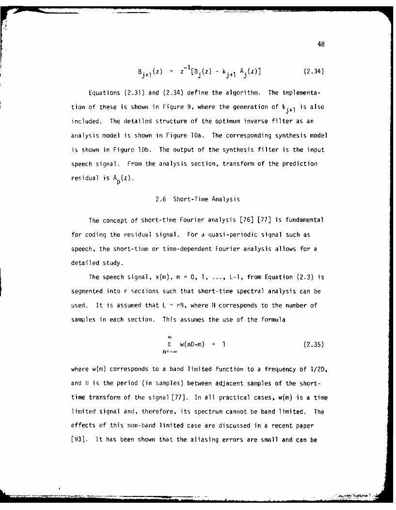
48
Bj+l(z) = z- [Bj(z) - kj+ 1 A (z)] (2.34)
Equations (2.31) and (2.34) define the algorithm. The implementa-
tion of these is shown in Figure 9, where the generation of kj+ 1 is also
included. The detailed structure of the optimum inverse filter as an
analysis model is shown in Figure 10a. The corresponding synthesis model
is shown in Figure lOb. The output of the synthesis filter is the input
speech signal. From the analysis section, transform of the prediction
residual is Ap (z).
2.6 Short-Time Analysis
The concept of short-time Fourier analysis [76] [77] is fundamental
for coding the residual signal. For a quasi-periodic signal such as
speech, the short-time or time-dependent Fourier analysis allows for a
detailed study.
The speech signal, x(m), m = 0, 1, ..., L-l, from Equation (2.3) is
segmented into r sections such that short-time spectral analysis can be
used. It is assumed that L = rN, where N corresponds to the number of
samples in each section. This assumes the use of the formula
E w(nD-m) = 1 (2.35)
where w(m) corresponds to a band limited function to a frequency of 1/2D,
and 1) is the period (in samples) between adjacent samples of the short-
time transform of the signal [77]. In all practical cases, w(m) is a time
limited signal and, therefore, its spectrum cannot be band limited. The
effects of this non-band limited case are discussed in a recent paper
[931. It has been shown that the aliasing errors are small and can be

49
A (Z) +Aj. 1(Z)
0 +.
B (Z) J-+j.I
CORRELATORTGENERATE
Kp1 Rj+I
Figure 9. Detailed Structure of PARCOR Implementation forjth Stage

50
N ~ rCJ
a)N
+N
+I
++ I--- I
41 c/)
-t +
N~N+
wX
CD
-i-I +
Nr cNT -< < >1
x) >!

51
neglected if D is properly chosen. For a Hamming window, D = (N/4) [77].
In addition to the aliasing errors, end effect errors have to be consid-
ered also [94]. This is necessary since L if finite. The LPC analysis
is applied to the windiwed signal resulting in the windowed residual
signal. The overlap-add of this signal is the residual signal, which has
error identified earlier.
The short-time Fourier transform of the residual signal ef(m) can be
defined as [67]
J k j w -J nkXn(e ) = [ef(m) w(nD-m)] e (2.36)
1n1= -
where wk = (2 k/N), k 0, 1, ... N-l, and w(m) corresponds to a window.
For a particular value of n, Equation (2.36) can be implemented using
FFT. This is used in this thesis. A brief review of this is presented
below.
Let
en (in) ef(nD+n) w(-m) -- < m (2.37)
Using this in (2.36),
Jwk J~kin -Jkn (.8Xn(e en(m) e e (2.38)
Further, let m = Nr+q, - r w, 0 • q _ N-1. With these,
jw k N-1 -JU(,k(Nr+q) _ knX n(e ) I: [: en (Nr+q) e ] e (2.39)
r=- q=0
JwkNrNoting that e = 1,

52
jwk N-i -jk q jWk n
Xn(e k) = E [ : e n(Nr+q)] e e (2.40)q=O r=--
I For simplicity, let
Un(q)= e en(Nr+q) 0 1 q < N-I (2.41)
Note that u n(q) is periodic with period N. Now Equation (2.40) can be
written, and is
Jk - j(11k n N-1 jW k q
Xn (e - e [ u n (q) e (2.42)q=O
Observe that X n (e ) is represented as e times the DFT of the se-
quence un (q). Therefore, (2.42) can be written as
j(Akn jU)k N-i -jWkqe Xn(e ) = un ((m-nD) )N e (2.43)
q=O
Equation (2.42) represents the OFT form, where (('))N corresponds to the
modulo N.
The following procedure can be used to compute (2.43).
1. The windowed sequence, en(m), can be computed from (2.37). The
sequence cen then be divided into r sections of N samples each, where in
this thesis, L = 4096, N = 256, D = 64, and r = 16.
2. The r-point DFT of un((m-nD))N can be computed to obtain (2.43)
using FFT.
The above procedure is given here for generality. Due to the limi-
tation of the disc space and to reduce computational time, a slightly
different procedure is used in computing the spectral analysis. The
residual signal is rectangular windowed to 256 points, spectrum analyzed
53
and then averaged. This is used only for phonemes discussed in the the-
sis. No overlapping was used. The errors associated with this method
are quantified in previously mentioned references [93] [94].
2.7 Implementation of Operations for the
Calculation of the Prediction Residual
In this section, the formulation of the prediction residual from the
speech input is presented. The implementation of the operations to cal-
culate the prediction residual represents the analysis model for LPC. The
analysis model consists of the speech as the input, the vocal tract model,
the correlation coefficients and the residual as the output.
The analog speech signal is band limited to 3600 Hertz using a second
order Butterworth filter. This signal is digitized at the rate of 8000
samples/second. The algorithm for digitization is named DIGITIZ and the
computer program is included in Appendix B.
The results in the last section are used to obtain the windowed dig-
itized data. This allows to process the speech in short segments. The
underlying assumption for most speech processing schemes is that the prop-
erties of the speech signal change relatively slowly with time [67]. This
assumption leads to short-time methods which isolate the signal during the
segment of windowing. The window is a 256-point Hamming window and is
overlapped at 64-point intervals. The windowing is computed by program
WINDOW in Appendix B.
The windowed signdl is passed to program AUTO [7]. This program uses
the autocorrelation method for solving the matrix equation (2.10) for the
predictor coefficients [61]. The other matrix values solved for are the
J - -..+ T ."--....... . . . ... . . . s, 2 ',? .
I -
54
reflection coefficients or PARCOR coefficients. These values are passed
for use in the lattice formulation.
The lattice method represents a recursive algorithm for a solution
of the prediction residual. This method guarantees stability. Note that
the PARCOR coefficients are bounded. The program to calculate the resid-
ual by the lattice formulation is INVERS and is included in Appendix B.
Figure 11 illustrates a block diagram showing the sequence of opera-
tions related to the calculation of the prediction residual, ef(n).
2.8 A Novel Approach to Pitch Extraction
2.8.1 Types of Problems Associated with Pitch
Extraction
The pitch extractor is of prime importance in most speech processing
systems, as the pitch is one of the basic parameters in speech analysis
and synthesis studies. In low-bit rate systems, it is an essential com-
ponent [2] [7]. Speech with a constant fundamental frequency is perceived
as a monotone or of a synthetic nature; variable pitch lends to speech a
melody. An accurate pitch extractor is a challenging area of speech pro-
cessing.
The difficulty in accurately determining pitch is due primarily to
the time varying aspects of the glottal excitation. Since the model of
the vocal tract assumes quasi-periodic changes occurring along the acous-
tic tube, the glottal response is not predicted accurately. This innac-
curacy is due to the nonuniform train of periodic pulses that occur with
the golttal waveform. The simple model of the vocal system excitation,
i.e., periodic uniform pulses or Gaussian noise, eases the measurement of
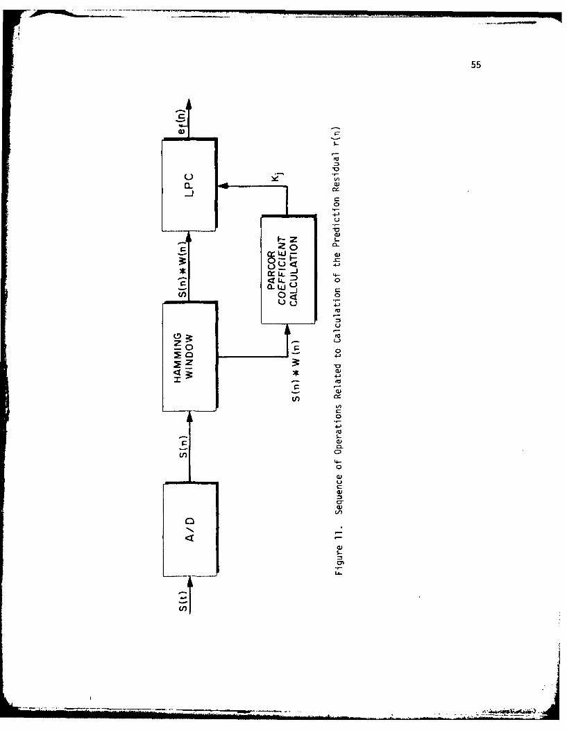
55
Ln
cr -J
.0
t
CD
0
C:)
4+.-0
a)
(UV)
7N.~
S)
a)

56
of the period of the pitch. However, when the pitch and the waveform are
changing within a period which occurs with frequency shifts, difficulty
arises.
The second problem associated with the measurement of pitch is due
to the nonseparability of the vocal tract model from the glottal excita-
tion. That is, the separation of the formants and the fundamental fre-
quency may not be possible and therefore the detection of the pitch
period is difficult. This interaction can be seen most often during
transitional regions of formants when the articulatory elements are
changing.
The third problem is the detection of the beginning and ending of
the pitch period. Part of this problem occurs in the definition of be-
ginning and ending of the pitch period. In examining the speech wave-
form, it is necessary to always be consistent with the method because
different definitions will often lead to different results. This is seen
in Figure 12. In Figure 12, one can detect the period of zero crossings
before the maximum peaks or detect the period between the maximums. How-
ever, the two methods do not always give the same answers. The discrep-
ancy between the two is due to the slowly time-varying properties of
glottal excitation.
The fourth problem that arises is the decision to ascertain which
segment of speech is voiced or unvoiced. In particular, some algorithms
have problems distinguishing between low-level speech and unvoiced speech.
In transitional analysis, it is difficult to pinpoint the difference
between the two.
In addition to the above problems, the pitch detection is hindered
further when the signal is a transmitted speech signal. During the

.lo
57
AMPLITUDE
....ERODBETWEENMAXIMUMS
kPERIOD BETWEENZERO CROSSINGS-
Figjure 1 . Two ilethods of Dctcrrninin PiLch Per-iod

58
transmission of a speech signal over a telephone line, there are degrada-
tions that occur that can change the signal to make pitch detection dif-
ficult. These include: 1) phase distortion, 2) amplitude modulation of
the signal, 3) crosstalk between messages, 4) clipping of high-level
sounds. Furthermore, as the signal travels through the telephone lines,
the lines act as a bandpass filter with approximate band edges f1 = 200
Hertz and f2 = 3200 Hertz. The fundamental frequency is usually less
than 200 Hertz and therefore is removed by the bandpass action of the
line. The pitch must be regenerated by using harmonics.
The next section discusses advantages and disadvantages associated
with the use of the prediction residual for pitch extraction.
2.8.2 Advantages and Disadvantages for Using
the Prediction Residual as a Source for Pitch
Extraction
The prediction residual solves the problem of vocal tract excitation.
Earlier, it is stated that there is inaccuracy in determining glottal re-
sponse when using the simple model for excitation. When using the two-
source model fo, the vocal system excitation, i.e., quasi-periodic pulses
and random noise, a simple algorithm can be used for extraction of pitch.
The residual can be used as a single source as an approximation to the
glottal excitation, and, therefore, a simple method can be used to employ
the residual to extract pitch.
It is well known that the residual represents the deconvolution of
the speech from the vocal tract [7]. For each vocal tract configuration,
a different set of formants and a variation in harmonics of the fundamen-
tal frequency in the spectrum is acquired. The pitch markings are
-I-* ~

59
determined by residual spikes in the time-domain. This can be used to
extract the pitch accurately.
The advantage of an accurate estimation of pitch will aid to the
perception of speech. Any enhancement to perception is important to any
analysis-synthesis speech system. The discussion which follows includes
other reasons for using the prediction residual as a source for pitch
extraction.
Referring to Figure 12, it is shown where errors can occur when the
speech signal is used for pitch extraction. Figure 13 shows the residual,
over 256 samples, characterized by spikes which represent the pitch per-
iod. It can be seen that it is not necessary to account for the zero
crossings or maximums. It is simply a matter of tracking absolute maxi-
mums within the range of the established pitch period. It has been shown
that if the interval of analysis is small enough the residual can be used
to extract pitch accurately [28]. Future transmission rates will require
a system that can do an acceptable performance for extracting pitch.
An application for using the residual signal for pitch extraction is
with embedded coding. The advantage with the residual signal is that an
absolute pitch can be determined in a frame. At higher transmission
rates, the coding of the residual can be accomplished more efficiently.
Therefore, a pitch extraction method can be employed easily. However,
it is not feasible to transmit the residual with low transmission rates;
consequently, the higher rates must extract the pitch and transfer this
to the lower rates. Since the residual demonstrates a very accurate
representation of the pitch, the frame-by-frame analysis of the pitch
from the prediction residual would enhance pitch in an embedded coding
scheme.

60
10-
5
CO~ IV .11
~10 0.08 0.16 0.24 0.32
TIME INTERVAL X 10-1Figure 13. Prediction Residual Waveform for Phoneme /ae/
over 256 Sample Segment
61
However, a disadvantage associated with the residual may occur in a
high noise environment. It has been shown earlier that the residual is a
combination of periodic and noisy signals. In a high noise environment,
the noise may overcome the residual signal. If the noise has amplitude
in the range of pitch markings, the signal would require enhancement to
extract pitch adequately. On the other hand, low noise contributes to
the flatness of the spectrum of the signal and enhances pitch extraction.
Several advantages and disadvantages have been discussed. It can be
readily seen that the residual is an ideal signal for extraction of the
pitch. The next section discusses the implementation of the pitch extrac-
tor.
2.8.3 A Novel Pitch Extractor
The last few sections have described the prediction residual as the
result from the linear prediction analysis. It has been shown that the
prediction residual contains much information needed for extracting pitch.
It is a simple problem to pick appropriate peaks to extract the pitch.
It is this problem of pitch extraction that has interested many authors
recently.
Examining Figure 13, a repetitive waveform is seen at the period
called the pitch period. Note that the waveform has a noisiness which
implies a flat amplitude spectrum. It should be noted that for voiced
sounds there are other peaks that are also repetitive. These are evi-
dence of the formant frequencies. They are somewhat dampened; however,
this is to be expected since the linear predictive filter has the charac-
teristic of spectrally flattening the signal.
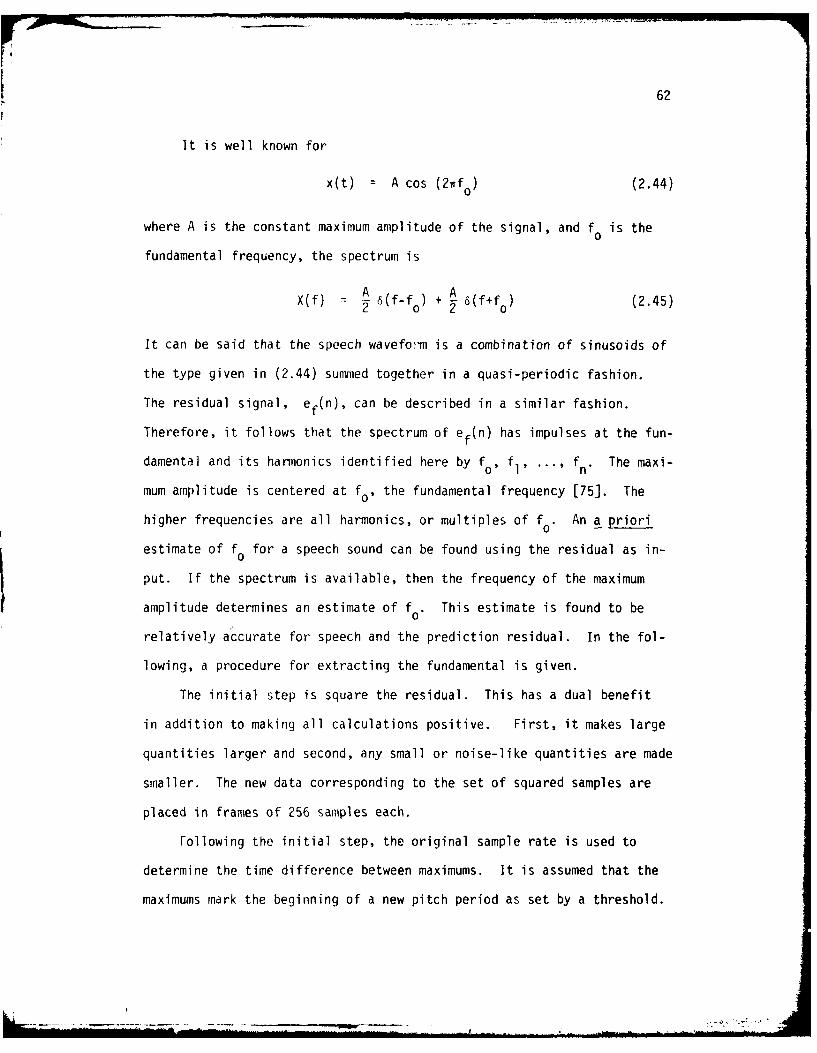
62
It is well known for
x(t) = A cos (2f o ) (2.44)
where A is the constant maximum amplitude of the signal, and f0 is the
fundamental frequency, the spectrum is
A AX(f) y 6(f-fo) + - 6(f+f ) (2.45)
It can be said that the speech waveform is a combination of sinusoids of
the type given in (2.44) summed together in a quasi-periodic fashion.
The residual signal, ef(n), can be described in a similar fashion.
Therefore, it follows that the spectrum of ef(n) has impulses at the fun-
damental and its harmonics identified here by f0, f15 ... 5 fn" The maxi-
mum amplitude is centered at f0, the fundamental frequency [75]. The
higher frequencies are all harmonics, or multiples of f o An a priori
estimate of f0 for a speech sound can be found using the residual as in-
put. If the spectrum is available, then the frequency of the maximum
amplitude determines an estimate of f 0 This estimate is found to be
relatively accurate for speech and the prediction residual. In the fol-
lowing, a procedure for extracting the fundamental is given.
The initial step is square the residual. This has a dual benefit
in addition to making all calculations positive. First, it makes large
quantities larger and second, any small or noise-like quantities are made
smaller. The new data corresponding to the set of squared samples are
placed in frames of 256 samples each.
Following the initial step, the original sample rate is used to
determine the time difference between maximums. It is assumed that the
maximums mark the beginning of a new pitch period as set by a threshold.

63
The threshold is used to select the next maximum. The data set is passed
through a peak picker. The peak picker uses the threshold to determine
the next peak (maximum). The time between the two peaks is calculated by
a differencer function. The system is ready to set a pitch value from
the time between the two peaks.
At this point, the a priori estimate of the pitch and the pitch
value from the differences are averaged. An error check is made for
erroneous pitch values. The error check compares a range of pitch from
a low to a high value. Should the averaged value be less or more than a
set threshold, an update is sent to recalculate the last averaged pitch
in the frame. The process is continued until the end of the frame where
the pitch is set. The procedure for estimating pitch is shown in Figure
14. The next section discusses the results in using the pitch extractor.
2.8.4 Pitch Extraction Results
The PITCH program was applied to 39 phonemes, including 16 vowels
and diphthongs and 23 consonants. Each sound was held from one-quarter
second to one second by a male speaker at normal intensity. Recordings
were made on a SONY Model TC-1O6A tape recorder under anechoic conditions.
The sounds were low-pass-filtered by a Butterworth filter with a cutoff
frequency of 3600 Hertz and samples at 8000 Hertz with nine quantization
bits and one sign bit. The computer system quantization level setting
was ±10 volts. This gave a quantization level of 20 millivolts. The
digitized sound was sampled for 1.5 seconds using 12000 data points for
storage. With a limited computer system memory, the beginning of the
sound was found and 4096 points were saved. The sound was stored for
later use and labeled with an appropriate name. Due to the processing

64
PITCH LSTIMATIOIN
START
e:f ()
SQUARE SPECTRAL
FUNCTION ESTIMATE
e2 (n) R(k)_Cf a FIND
VALUE
SE A PRIORI
T-RSTL ESTIMATE
THRSHLD fn)MoK R(k),,,, FUNDAMENTAL
AN DDIFFERENCEFUNCFION
SET NE WAVG. PITIH j- -_____
P(m)
IUPDAI JCHEFCK FOR
I. VARIANCE OFITCH
'NO
NO CHEICK FOR YFS ET SSETE-ND OF - ' PITCH SO
Figure 14. Block Diagram of Pitch Extraction Method

65
of the INTERDATA 70 computer system, all processing in program PITCH is
done in 256-point blocks.
The unified rek'irsive solution to solve Equation (2.10a) is by pro-
gram AUTO [7]. The efficient resursive solution was discussed in an
earlier section. The program INVERS processes the data. The residual
data is stored for use in the program FFTMGR. The computation of the
spectrum is performed in this program. Spectral values are stored for
use in PITCH.
Samples can be plotted for any segment of the sound to aid in visual
determination of the pitch period. An example is shown in Figure 13.
The results show that the method presented here is an adequate and accur-
ate method for determining pitch period. It is compared to Peterson and
Barney's data [111]. Table III gives a comparison between this data and
the results obtained from this method. From this table, it can be seen
that the results are good. The voiced/unvoiced decision is not a product
of PITCH. The FFTMGR routine produces an energy level for the determina-
tion of voicing. Voicing errors were made 25 percent of the time. This
is due to Lhe fact that the threshold is set to a low level. However,
the error check will restrict any wide variance of pitch. If the calcu-
lated fundamental frequency is larger than a set threshold value of 400
Hertz, then the corrcsponding sound is considered as an unvoiced sound
and no further calculations are made. These two checks allow for accur-
ate measure of pitch and voiced/unvoiced decision.
Error-free pitch estimation is critical to the overall performance
of any low-bit rate coding system. Coding systems that incorporate the
residual signal for estimation of the pitch are accurate and adequate.
Accuracy can be enhanced by using the residual in a minimum noise

66
environment. The residual signal formulates a true pitch per frame that
can be used at low, synthetic transmission rates. There are several rea-
sons that have been discussed to show that this is a novel approach to
pitch extraction and is sunarized below. First, it is a two-stage method
that estimates the residual spectrum and uses time samples of the residual
to calculate the approximation of the pitch. Second, the calculation is
done by a thresholding technique which uses the square of samples. Fi-
nally, the extraction of the pitch includes an error check that estimates
wide variances of the pitch during each frame. From these, it can be
seen that this method can be considered as a hybrid technique.
TABLE III
COMPARISON OF FUNDAMENTAL FREQUENCIES
Frequency (Male)Fundamental from
from Proposed Method ofPhoneme Peterson-Barney [111] Pitch Extraction
/i 136 129
/I/ 135 130
130 125
/x! 127 135
/u/ 124 123
/l/ 129 135
Ad 137 126
/U/ 141 151
/A/ 130 123
133 140

67
2.9 Sunmary
In this chapter, the characteristics of the prediction residual were
presented. There is a parallel between the glottal waveform and the re-
sidual. The mechanism of speech production and a model of the vocal
tract is discussed. Short-time spectral analysis is presented. A review
of linear prediction analysis is discussed. A description of the imple-
mentation of operations for the calculation of the prediction residual is
discussed. A novel approach to pitch extraction is presented.

CHAPTER III
SUB-BAND CODING OF THE PREDICTION RESIDUAL
3.1 !-troduction
The average rate that speech is conveyed between humans is about ten
phonemes per second. It has been shown that the information rate of
speech does not exceed 60 bits/second [2] [67]. For the information con-
tent to be preserved, the human must be able to extract the representation
of the speech signal at this rate. It is important that the speech is
intelligible to the listener, and this aspect is the fundamental consid-
eration of coding speech.
There are two concerns in coding speech signals. First, the message
content of the speech must be preserved. The content includes linguistic
rules to form thoughts for humans to communicate. Second, the speech
signal should be represented so that it can be transmitted. At the re-
ceiver, the signal should contain the message without serious degrada-
tions.
The interest in speech coding has led researchers to consider tech-
niques that enhance signal quality, reduce transmission rate and cost,
without considering the complexity of the coding algorithm [64]. The
principle is to enhance the perceptual aspects of speech through the
coding method. In this chapter, some basic ideas associated with speech
coding are discussed. These include transform coding and sub-band-coding.
68

69
Since the speech sounds are characteristically different than most acous-
tic sounds, it is necessary to consider the properties that include the
formants and energy of phonemes. Perceptual aspects that contribute
transitional cues for humans to discriminate and differentiate speech
sounds are discussed in this chapter. It is known that when human lis-
teners are exposed to speech, available to them are a set of responses
that are highly over-learned [65]. The minimum discrimination necessary
for absolute differentiation of speech sounds is discussed. Recently,
speech coding techniques have contributed efficient methods to enhance the
coding of speech signals with few degradations. This chapter discusses
some of these methods in Section 3.2. Section 3.3 presents a discussion
of the transform coding. Section 3.4 presents the method of sub-band
coding in detail. Section 3.5 discusses the determination of frequency
bands by the Articulation Index. Section 3.6 presents aspects associated
with transitional cueing information for the preception of certain pho-
nemes. Section 3.7 discusses perception of intelligible speech. Section
3.8 describes the basis for coding the prediction residual at the rate of
9600 bits/second.
3.2 Coding Methods
The oldest form of speech coding device is the channel vocoder inven-
ted by Dudley [78]. Each of the channels has center frequency wk" For
each of the channels, the time-dependent Fourier transform is represented
as a cosine wave with center frequency w k which is phase and amplitude
modulated corresponding to the magnitude and phase angle, respectively of
each transform. Therefore, each channel is thought of as a bandpass

70
filter with center frequency wk and impulse response w(n). This is shown
in Figure 15.
The analysis section consists of a bank of channels as in Figure 15
with frequencies distributed across the speech band. Figure 16 shows a
complete channel vocoder analyzer.
The basic diagram for the synthesizer is somewhat different. The
specific channel controls the amplitude of its contribution to a particu-
lar channel; while the excitation signals control the detailed structure
of the output of a given channel. The voiced/unvoiced decision serves to
select the appropriate excitation generator, i.e., random noise for un-
voiced speech and pulse generator for voiced speech. A block diagram is
shown for the synthesizer in Figure 17. Channel vocoders operate in the
range of 1200 bits/second to 9600 bits/second. They are also referred to
as source coders and produce speech of a synthetic nature when at bit
rates below 4800 bits/second.
A major contribution of a channel vocoder is the reduction in bit
rate; however, direct representation of the pitch and voicing information
is not achieved. Therefore, this can be considered as a weakness.
The LPC vocoder is a very important application of linear predictive
analysis in the area of low bit rate encoding of speech. It is shown in
Figure 18.
The basic LPC analysis parameters consists of a set of P predictor
coefficients, the pitch period, a voiced/unvoiced parameter and a gain
parameter. The vocoder consists of a transmitter which performs the LPC
analysis and pitch detection. These parameters are coded and transmitted.
They are decoded and synthesized to output speech. This category of
- -r -------- ______________
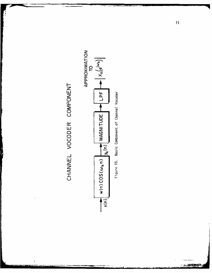
71
<
0
a-zLiJ U- Lz a- ~o -J 0
00
0
-
LLJ 4-)
0LuLo 0
0)
LU22 <:
I (/)d

72
_ z
4p az Z C
w w
ww
< 0)
- 0
LiJ W -
0 4-0
0 a
wz -
2 D 0
Co 0 0SL
w w
u:- LLZ 00 .

73
>0D
NN
LAJ
0 -
Z z )
o m
0:

74
z
0ow
0 JI
w0 z
z00C-)-
LJJI
LLJ 0
_o u
z

75
coding is of the vocoder type. In the following, the discussion of vari-
ous aspects is included.
Speech coding can be divided into two broad categories, waveform
coders and vocoders [79]. There has been some metion of a few types of
vocoders earlier. Waveform coders generally attempt to reproduce the
original speech waveform according to some fidelity criteria. On the
other hand, vocoders model the input speech according to some speech pro-
duction model; then, synthesize the speech from the model. The basic
make-up for coding the prediction residual in this thesis is of a vocoder
model. However, techniques of wav form coding are also used. It has
been shown that waveform coders tend to give better quality speech that
is robust; whereas, vocoders tend to be more synthetic [64] [79]. Bor-
rowing from the techniques of efficient waveform coders, it is conceiv-
able to define an acceptable coding algorithm to meet quality standards
at low-bit rates of transmission. A primary interest has been to produce
the transmitted speech with the minimum bit rate and still meet accept-
able quality [80]. Previously mentioned were methods available to date
for coding of the residual. Efficient methods to improve the coding
techniques are presented for coding the prediction residual.
It has been recognized that there are two efficient methods of wave-
form coding [79]. These are: (1) transform coding (TC) [81] and (2)
sub-band coding (SBC) [36] [371. These are characterized as frequency-
domain coders, whereas examples of PCM, differential PCM, and DM are the
time-domain coders. Frequency-domain coders are perceptually better than
time-domain coders because they tend to exploit the pitch of the speech
waveform for bit rates below 16000 bits/second. They tend to look at the
spectrum of speech in blocks, whereas the predictive systems look at

76
adjacent samples. These two methods will be explained in detail in the
next two sections.
3.3 Transform Coding
With transform coding (TC) [81], the system of speech samples is
grouped into blocks, where each block corresponds to the windowed segment
of the speech signal. These blocks of speech are transformed into a set
of transform coefficients; then, the coefficients are quantized indepen-
dently and transmitted. An inverse transform is taken at the receiver to
obtain the corresponding block of reconstructed samples of speech (see
Figure 19).
A basic assumption in this method is that the speech source is sta-
tionary and has a variaice of o2 . The successive source output samples
are arranged into the N-vector X; this vector X is linearly transformed
using a unitary matrix A, i.e.,
Y = AX (3.1)
where A, in general, is complex, and
AA* = I (3.2)
where * denotes the transpose conjugate. The elements of Y are the trans-
form coefficients. These are independently quantized, yielding, Y. The
vector Y is transmitted to the receiver and then inverse transformed.
Then
X = A Y (3.3)
Since the vector X is reconstructed output, distortion is involved. For
unitary matrices the averaged mean-squared overall distortion of the
.

77
IMPLEMENTATION OF TRANSFORM CODING
(After Zelenski and Noll, 1977).x

78
transform coder is equal to the (udntization err(Jr [82]
D = E{(X - X)T (X - X)}b N
E (Y - Y) (Y - Y)) (3.4)
N
There Ef I represents the expectation. The minimization of D will yield
an optimum bit-assignment rule arid an optimum transform matrix A [81].
Let Ji be the number of bits/sample needed for the coefficient Yi (an
entry in the Y vector) of variance o? so that the mean-squared distortion1
.= E[Y i - Yi)2] is not exceeded. Then [82]Di i
i + log2 [ -D- ] (3.5)
where 6 is a correction factor that takes into account the performance of
a practical quantizer. The optimum number of bits for the quantizer can
be obtained by minimizing the average distortion
1 Nl Di (3.6)
with the constraint of a given average bit rate
1 NR J. constant (3.7)N i=l1
The optimum bit. assignment is [81]
J. + loq bit/sample i =1, 2,..., N
(3.8)
The averdqe distortion is found to be
--'- - -:- -:= -- :-:-- - : _i ........ .. -' l l R N I I R J I l !n I .. . .

79
0 2' 2-2R r IT 21IN (3.9)
Here the distortion introduced by the transform coding scheme depends on
the distribution of variances. In addition, D is found to be the geomet-
ric mean of the variance. This leads to the solution of A matrix. Let
R and R be the covariance matrices of X and Y, thenxx yy
Ndet R o. (3.10)YY - il 1
and for any unitary matrix A
det R = det R (3.11)xx yy
In particulre, the variances o. are along the diagonal of Ryy; then,
Ndet R = A X. (3.12)
where >. are the eigenvalues of R . Therefore, the minimum distortion
is found if the variances, , are equal to the eigenvalues of Rxx [81].
The Karhunen-Loeve transform (KLT) has the property that c = i for all
i.
Other unique properties of KLT are: (1) transform coefficients are
uncorrelated, (2) the covariance in the KLT domain is diagonal, and there-
fore, the transform coefficients can be quantized independently without
the loss of performance [83].
It has been noted that the KLT gives optimun performance; however,
there is a lack of a last algorithm for the computation of the coeffi-
cients. In addition, the computation is quite complex. Since speech is
a quali-periodic signal, transform coding would not be efficient unless
AD-AC92 198 IR8 FORCE INST OF TECH WRIGHT-PATTERSON AFB3 OH F/r 9/,FICIENT COOING OF THE PREDICTION RESIDUAL. CU)rAEC 79 L L SURGE
VjEA~~~l.tT-Cl-9-235D N
mo mmmmm i

1111 i.Q I: *8 112.511111 1112.
'I1.6
MICROCOPY RESOLUTION TEST CHART
NAr(ONAL BURt4U Of STANDARDS 1963

80
adaptive methods are used. However, this area still needs additional
studies. Zelenski and Holl presented promising results. Tribolet and
others [38] have done additional work in this area also. Zelenski and
Noll experimented with the Walsh-Hadamard transform (WHT), the discrete
slant transform (DST), the discrete Fourier transform (DFT), and the dis-
crete cosine transform (DCT) to compare with the KLT. All these have
fast algorithms and are signal independent. Zelenski and Noll found that
the basis vectors of the OCT and KLT are close; however, the KLT is sig-
nal dependent. It has been shown that the performances of the DCT and
KLT are similar [84]. The studies of Tribolet and others found TC to be
complex and costly; however, this method proves to be superior when com-
pared to other systems [38].
3.4 Sub-Band Coding
It is desired to retain the basic components of speech composition
and phonemic quality. TC is a very efficient method of completing the
endeavor; however, due to cost and complexity, it was discarded. The
method of sub-band coding [36] has some very distinct advantages whereby
the original goal can be met in order to secure as much of the speech
signal as possible. One criterion, perceptual in nature, is the reten-
tion of transitional information. Also, the intelligibility of speech
can be maximized by the use of the Articulation Index [29], which is
discussed in Appendix C.
With sub-band coding the frequency spectrum is partitioned such that
each sub-band contributes accordingly to the speech intelligibility which
is quantified by the Articulation Index. The Articulation Index is a
weighted fraction representing, for a given speech channel and noise
L -..

81
condition, the effective proportion of the normal speech signal which is
available to a listener for conveying speech intelligibility [86]. The
speech spectrum can be divided into 20 frequency bands contributing 5 per-
cent each to the Articulation Index. In this case, the frequency spectrum
can be bandpass filtered in such a way that they contribute equally to the
Articulation Index. An example given by Crochiere and others (36] in
Table IV addresses a sub-band partitioning of four bands between 200 to
3200 Hz.
TABLE IV
SUB-BAND PARTITIONING EXAMPLE
Sub-Band No. Frequency Range (Hz)
1 200 - 700
2 700 - 1310
3 1310 - 2020
4 2020 - 3200
Obviously, there are other possibilities of partitioning the speech
band [37]. Each band contributes an equal 20 percent to the total Artic-
ulation Index. The total Articulation Index is 80 percent, which corre-
sponds to a word intelligibility of approximately 93 percent [36].

82
Sub-band coding has another advantage which involves quantization.
Each sub-band is quantized separately and each band contains its own dis-
tortion and, therefore, quantization noise could be considered separately
for each band [36]. Furthermore, because of the nature of the spectrum
of speech, the detectability of this distortion is not the same at all
frequencies.
Since the proposed method is based upon sub-band coding the resid-
ual, the presentation is in terms of the prediction residual, ef(k).
For the following discussion, assume that the sub-bands are parti-
tioned as shown in Figure 20. Let the width of each of these bands be
identified by
Wn = W n+l - On n = 1, 2, ..., N=4 (3.13)
where wrn corresponds to the edges of these bands. The implementation of
the sequence of operations leading from the residual to the coded output
for transmission is shown in Figure 21. Also, shown in Figure 21 is the
implementation at the receiver. From this figure, it follows that
r(k) = (efn(k) cos w n k) * hn (k) (3.14)
where e fn(k) corresponds to the output of the nth bandpass filter and
hn (k) corresponds to the impulse response of the nth lowpass filter. It
is clear that
W 2 n (3.15)
in order that the frequency bands are properly separated. Then r(k) is
decimated to the rate 2Wn from the original sampling frequency. This
signal is then encoded and multiplexed with the other channels. At the
receiver, the signal is demultiplexed, decoded, interpolated, demodulated

83 I
1' ICBAND
1 2 3 4
-
0-
4
-30
CO1 W 2 CO3 W4 WL5
FREQUENCY MkHO
Figure 20. Partitioning of Frequency Spectrum into Four Sub-Bands
(After Crochiere, 1976)

84
a
Li C
0 0
aot
to
:3
o 0
0
- 0 -
00a) +
3 C3

85
and bandpass filtered to give efn(k). This is shown in Figure 21. The
nth sub-band is then summed with other bands to produce ef(k), which is
the sub-band coded and decoded version of the signal. The total imple-
mentation of the system will be discussed later.
3.4.1 Sub-Band Coding and Transform Coding
Earlier it was pointed out that frequency-domain coders can be con-
sidered as a good basis for an efficient coder. In this section the re-
lationship between sub-band coding and transform coding is discussed.
Considering the ideal case, in which there are M sub-bands corre-
sponding to the M samples, let the discrete cosine transform (DCT) of the
residual signal, ef(k), k = 0, ..., M-l, be represented by [84]
M-1--- 0E ef(k)0o /I k0O
n = M, ... , M-1 (3.16)
-,- M-1 (2k + l)nnan k=O ef(k) cos 2M
Correspondingly, the residual signal ef(k) is given by
k) 1 M-I (2k + 1)nflef (k) =M an cos 2M k 0, ,..., M-1VW nil
(3.17)
which obviously corresponds to the inverse discrete cosine transform
(IDCT). Using
n 2k 2M (3.18)
in Figure 21, it is seen after modulation and low-pass filtering
r(k) = n k=O, I, ..., M-1 (3.19)

86
Since there are M sub-bands corresponding to the M frequencies, and since
r(k) is a constant, it follows that after the decimation only one point
is given for each band and that value is an. The encoder in Figure 21
codes the OCT coefficient. This points out the fact that in the ideal
case (i.e., filters and modulators are ideal), the sub-band coding will
be equivalent to the discrete cosine transform coding. Obviously, the
discussion above can be oeneralized for the case wherein there are N sub-
bands (N < M) rather than M.
It is clear that where the components in the sub-band coder are non-
ideal, the r(k) are not equal to an. Further work is necessary in quan-
tifying the difference between r(k) and an [85].
Noting the simplicity in the sub-band coder and also noting the re-
lationship between the transform coder and sub-band coder, the sub-band
coder is more practical.
3.5 Determination of Frequency Sub-Bands
Based on Articulation Index
The Articulation Index (AI) is a weighted fraction representing, for
a given speech channel and noise condition, the effective proportion of
the normal speech signal which is available to a listener for conveying
speech intelligibility [29].
In this section, the methods of determining how to achieve maximum
intelligibility based on using the AI are examined. There are two meth-
ods for computing Al. The first method, called the 20-band method by
French and Steinberg [86], is based on measurements or estimates of the
spectrum of the speech and noise present in each of the 20 continuous
bands of frequencies. Each band contributes equally to the speech

87
intelligibility. The second method, known as the octave-band method, is
derived from the first method. It requires measurements of the speech
and noise present either in certain one-third-octave-band or in certain
full octave bands.
Some researchers consider these two, i.e., one-third-octave-band and
full octave-band measurements, as different methods. The octave-band
method is not as sensitive to variations in the speech and noise spectra
as the 20-band or the one-third-octave-band method. An example where it
falls apart is in situations where an appreciable fraction of the energy
of the masking noise is concentrated in a band of frequency that is one
octave or less in width; under these conditions, the one-third-octave-
band or the 20-band method would be better to use.
The 20 frequency bands are those specified by Beranek for male
voices [87]. These bands are shown in Table XXIV in Appendix C. In order
to use the 20-band method to calculate the AI, the peaks of the spectrum
of the speech signal (PSS) must be approximated first. The level depends
on if the speech is spoken through earphones or a loudspeaker. There is
an adjustment to either case of -65 dB which is considered as the over-all
long-term rms sound-pressure level of an idealized speech spectrum. How-
ever, with the loudspeaker, an additional amount is adjusted according to
Table V [29]. This is due to the assumption that the room is semirever-
berant; whereas, earphones do not present reverberance.
These corrections are obtained from experiments conducted in a re-
verberant room using a loudspeaker and from experiments conducted in an
anechoic chamber [29].
Also an additional correction must be added to correct for the noise.
spectrum. This is shown in Table VI [29]. The noise that reaches the

88
listener's ear is assumed to be that of a steady-state nature. All
noises in the listener's environment and the noise in transmission systems
are combined to arrive at the noise spectrum level.
TABLE V
ADJUSTMENTS TO THE SPECTRUM OF THE SPEECH SIGNAL
Maximum Spectral Values Amount to beof Speech Signal Subtracted
85 dB 0 dB
90 2
95 4
100 7
105 11
110 15
115 19
120 23
125 27
130 30
The corrected noise spectrum (NS) has the effect of masking the
speech signal. The noise spectrum increases at a faster than normal rate
when the band sensation level of the speech sound exceeds 80 dB [86].
ihis band sensation level is defined as the difference in decibels between

89
the sound integrated over a frequency band and the sound pressure level
of that band when the speech sound is at the threshold of audibility in
an anechoic room. The increase in masking is taken into account in the
calculation of AI by adding to the PSS. If the band sensation level of
the sound exceeds 80 dB at the center frequency of a band, then the PSS
is increased by the amount that is shown in Table VI.
TABLE VI
ADJUSTMENTS FOR NOISE SPECTRUM
Band Sensation AddedLevel Amount
80 0
85 1
90 2
95 3
100 4
105 5
110 6
115 7
120 8
125 9
130 10
135 11
140 12
145 13
150 14

90
The noise spectrum level (NS) is compared to PSS at the mid-frequen-
cies of the 20 bands given in Table XXIV in Appendix C. Values that are
zero or less are set to zero. When PSS exceeds the noise by 30 dB, then
that difference is set to 30. This is due to the limitation on the dy-
namic range of speech [87].
The Articulation Index is defined as
AI = E Wn • (AA)max (3.20)n
where
(AA)max is the contribution from one band and has a maximum value of
0.05.
Wn is the percent of maximum contribution by any one band
and
Wn PSS - NS (3.21)
where 30 represents the dynamic range of the speech band and is a normal-
ized so that Wn is limited to unity. Therefore, for 20 bands, the normal-
ization is limited to 600. An illustrative example is given by Kryter
[29].
Consider the one-third-octave-band and octabe-band method. The cen-
ter and cut-off frequencies for these are shown in Tables VII and VIII
[291.
With the one-third-octave and octave-band methods, the correction
levels shown in Table V should be considered for signals received from
the loudspeaker. Also, the NS must be calculated from Table VI, and the
weighting factors need to be computed from (3.21) for each band. These
L ! . ... I
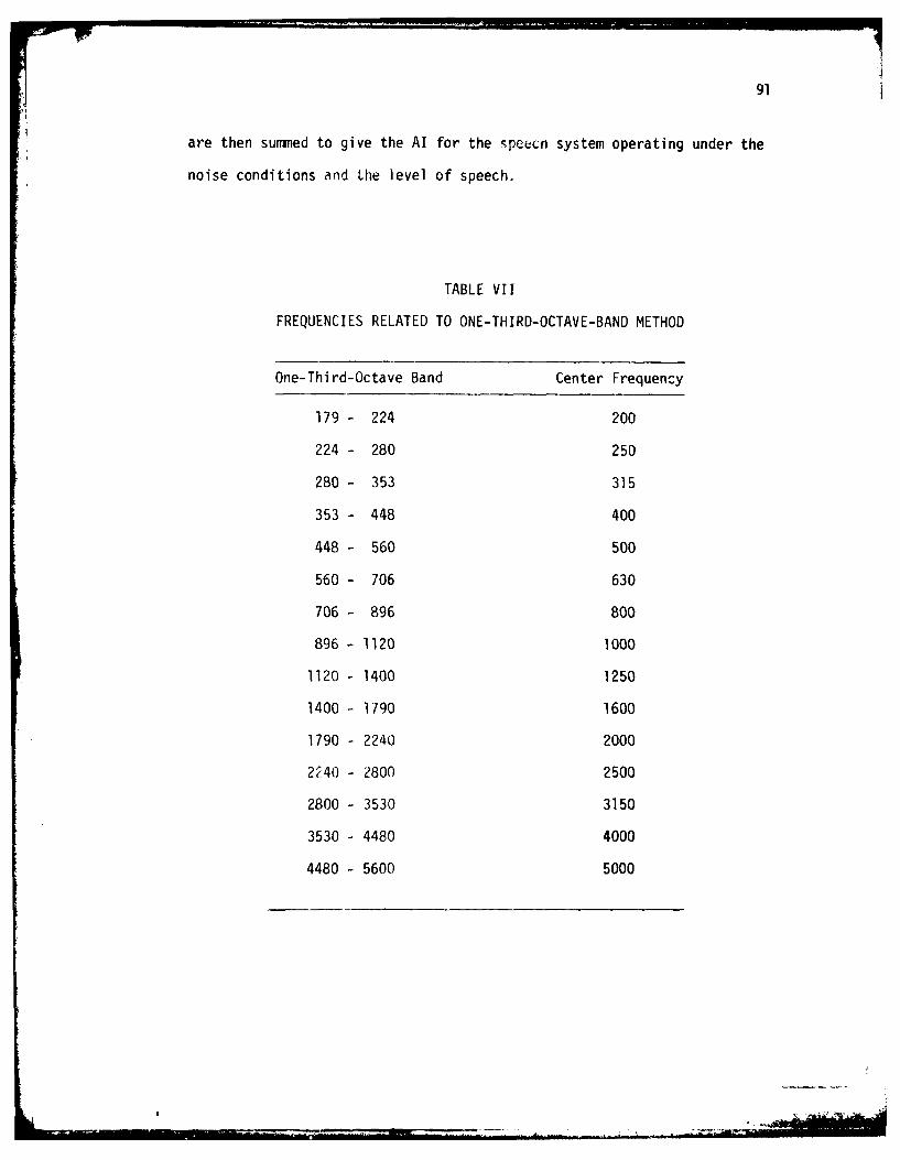
91
are then summed to give the AI for the speech system operating under the
noise conditions and the level of speech.
TABLE VII
FREQUENCIES RELATED TO ONE-THIRD-OCTAVE-BAND METHOD
One-Third-Octave Band Center Frequency
179 - 224 200
224 - 280 250
280 - 353 315
353 - 448 400
448 - 560 500
560 - 706 630
706 - 896 800
896 - 1120 1000
1120 - 1400 1250
1400 - 1790 1600
1790 - 2240 2000
2240 - 2800 2500
2800 - 3530 3150
3530 - 4480 4000
4480 - 5600 5000

92
TABLE VIII
FREQUENCIES RELATED TO OCTAVE METHOD
Octave Band Center Frequency
180 - 355 250
355 - 710 500
710 - 1400 1000
1400 - 2800 2000
2800 - 5000 4000
To consider how the different methods compare for the same speech
signal and masking noise, Kryter computed the AI for each of these meth-
ods. For 20-band method, AI = 0.38; for one-third-octave method, AI =
0.33; and for octave-band method, AI = 0.28. Since the 20-band method is
the basic method from which all others are derived, it provides the
"correct" AI and the others are compared to this AI.
The AI can be compared to estimated speech intelligibility scores as
shown by graph in Figure 22. It is noted that the intelligibility score
is highly dependent on the constraints placed on the message communicated.
The greater constraint (for instance, the smaller the amount of in-
formation content in each item of message), the higher the percent intel-
ligibility score for a given AI. No single Al can be used as a criterion
for an acceptable communication value. It is a function of messages
transmitted and the enunciation of the talker [29].
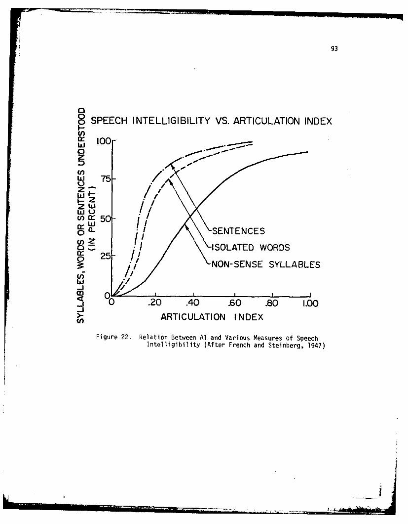
93
8 SPEECH INTELLIGIBILITY VS. ARTICULATION INDEXina: 100-
z
ISLZE WOD
WU,
0 .20 .40 .60 .80 1.0ARICLAIOAE WNDES
Fiur 222eainBewe5-ad aiu esue fSecInelgblt AtrFenhadSeneg 97
3.1 NON-SENSE SYLLABLE

94
The Articulation Index is a good quantitative measure of speech
intelligibility. Speech comunication can be enhanced by an equal appli-
cation of Al across the speech spectrum in the sub-band coding. In the
next section, the transitional cueing of phonemes, another aid that adds
to speech communication is discussed.
3.6 Transitional Information
The human speaks in an uninterrupted and continuous fashion to com-
municate thoughts. The underlying basis for communication is the pho-
nemic structure that connects itself by means of transitional cues for
the perception of certain phonemes [1]. It is the transitional informa-
tion that must be enhanced to aid the perception needed for absolute
discrimination of speech-like sounds [2]. Transitional cues are a set
of frequency shifts which occur in the second-formant region where a
consonant and a vowel join. The perception of a given phoneme is
strongly conditioned by the transitional information of its neighbors
[2].
The identification of phonemes has been studied under various con-
ditions by a group at the Haskins Laboratories [1]. Many of their ex-
periments have used synthetic syllables. The combinations of syllables
included consonant-vowel (CV) syllables. The consonant is usually a
stop out of a group of phonemes with the same voicing. The vowels were
maintained at two formants. Further work has been done by Rabiner [883
for synthesis of phonemes by rules. These concluded that one frequency
variable of the consonant was generally adequate to distinguish that a
consonant of the group was uttered. To further distinguish the

95
consonant, the stop-vowel formant transitions were necessary to perceive
the consonant.
Figures 23(a) and 23(b) illustrate the stop-vowel formant transi-
tions. In Figure 23(a), the vowel /a/ has first and second formants
occurring at 700 Hz and 1200 Hz respectively. It is seen that the con-
sonants /b/, /d/ and /g/ demonstrate a different rise or fall in the
second formant region. The second formant varies because each consonant
has a different place of articulation. The place of articulation for
/b/, /d/ and /g/ are front, middle and back, respectively. It is seen
in Figure 23(a) that the consonants appear to commence from some trajec-
tory determined by their place of articulation.
The trajectory point is further illustrated in Figure 23(b). This
figure uses the consonant /d/ and three vowels, /a/, /i/ and /u/. It is
shown that the consonant /d/ has a loci of points that commence in the
region of 1600 Hz for the second formant. It has been shown that con-
sonants exhibit this property of transition from a particular frequency
to the steady-state value of the vowels [1].
The consonants that are perceptually heard with falling second for-
mants to the vowel /a/ are /d/ and /g/. The consonant /b/ is heard with
a rising second formant to the vowel /a/. It is noted that a shift in
second formant frequency is bounded. With falling transitions of the
second formant, /g/ is heard for steady-state levels of frequency between
2280 and 3000 Hz; however, between 1320 and 2280 Hz the sound could be
/g/ or /d/; and, below 1320 Hz, it is identified as /d/ [1].
The importance of second-formant transitions is shown for perceptual
purposes. Differences in the acoustic speech signal are due to the exci-
tation and vocal tract configuration for different consonants. These

96
t o toVcc
(*c
0;
o 0 0 0L
00
00
C.-
0
z
00
toN N Pqo i 0 d 0 m4
N w 0
00r
o 0 0 0 a 0
cc 0 0 8 0 0 0 LL
-J (ZIl) AO3nMO8.

97
will differ as shown in Figure 23 by the transition regions. The con-
sonant transitions are the principal cues for the perception of a parti-
Ular consonant. The transition occurs because the vocal tract has one
shape for the vowel and one shape for the consonant. The change in the
vocal tract and the effect that the glottal pulse has on vowels has been
addressed recently [12]. Later, the coding aspects of transitional in-
formation will be discussed.
3.7 Relation of Perception
to Intelligible Speech
A topic that has been mentioned several times before is perception.
Perception related to the Articulation Index and transitional information
together for discrimination of speech sounds. A quantitative description
of speech perception is not possible. However, in a qualitative sense,
speech perception can be enhanced when the intelligibility of speech is
increased. In this section, several aspects of speech perception will be
discussed to show the need to address this subject.
Speech perception can be defined as the ability for humans to dis-
criminate and differentiate the character of speech sounds. Discrimina-
tion is examined along fundamental dimensions of the hearing mechanism
and, in general, one dimension at a time. The ear takes measurements and
makes differential comparisons. These comparisons may be of frequency
and intensity. The over-learned senses of the brain distinguishes the
speech from other periodic waves. Further, the speech must be broken in
to its discrete elements, the phonemes. Once the signal is perceived as
speech, there are other factors that determine the fundamental character-
istics of recognizing intelligible speech.

98
The ability to recognize and understand speech determines intelligi-
bility. The intelligibility of speech may be affected in several ways
[86]. These may include echoes, phase distortion, or reverberation. Un-
natural sounding speech can influence intelligible understanding of
speech sounds. The intensity of thespeech may affect intelligibility of
speech received by the ear. Noise in a transmission medium may affect
intelligibility by masking the speech. The talker and listener have
several factors that can cause unacceptable intelligibility related to
the speech [86]. These are given below:
a. The basic characteristics of the speech can be destroyed.
b. The electrical and acoustic instruments which operate between
the talker and the listener may not be adequate.
c. The condition under which the communication takes place may not
be acceptable.
d. As a result of c., the behavior of the talker and listener may
be modified by the characteristics of the communication system.
The perception of intelligible speech is related to the amount of
information spoken. This is shown in Figure 22. The exactness with
which the listener identifies speech sounds is related to the size of
the vocabulary and the sequence or context of the message. As seen from
Figure 22, the more predictable the message is, the better the intelli-
gibility. It has been shown that as the vocabulary size increases, a
higher signal-to-noise ratio is necessary to maintain performance [2].
Perceptual aspects of speech are influenced greatly by semantics
and context. The ability to predict the speech utterance enhances intel-
ligibility. The grammatical rules of a language are part of the human
over-learned senses [65]. Consequently, the language prescribes a
______ i

99
certain allowable sequence of words. The semantic factors occur as part
of the rules because certain words must be associated with meaningful
units [66]. It has been shown that intelligibility of speech is substan-
tially higher when a grammatically correct and meaningful sentence is
spoken than when using the same words randomly [65]. The over-learned
senses reduce the number of alternative words from the context, and
therefore, the listener has improved intelligibility.
The application of speech perception is an adaptive process. The
listener uses the detection procedure within the reception system of the
ear to determine the speech communication process. The listener can
absolutely identify speech when given the basic sound elements of the
speech. The sound elements are discriminated and differentiated from
other periodic sounds to perceive speech. If the speech is intelligible,
the exactness is not only related to how good the transmission medium is
but also to the length of the utterance and its context. These concepts
are applied in the next section to aggregate a coding algorithm for
transmission of perceptually enhanced speech.
3.8 Basis of Coding the Predictional Residual
A coding method is presented to perceptually enhance the speech.
The method uses sub-band coding (SBC) for coding the prediction residual.
Besides SBC being conceptually simple, it has the additional advantage
that each sub-band is quantized separately and each band contains its
own distortion. It should be pointed out that the input to the sub-band
coder is the residual signal rather than the speech signal. Some of the
reasons for this approach are:
a. A more efficient bit distribution based on energy/frame.
a"_

100
b. A more pronounced pitch information in the residual signal, and
c. An ideal input for the synthesizer at the receiver.
In an earlier section, the advantages of using the Articulation In-
dex in SBC have been discussed. Each sub-band is selected such that each
contributes equally to the Articulation Index [36]. However, it has been
shown that "satisfactory" performance can be expected if this equal con-
tribution to the articulation criterion can be met within a factor of
two [37] [87]. This relaxation of the criteria was allowed for integer-
band sampling with good results [36] [37]. That is, the sub-bands are
between mi 0i and (mi +1) wi, where mi is an integer. The method has
popularity because it eliminates the need for modulators. Even though
the integer-sampling method requires less hardware, the selection of sub-
bands using the articulation criteria would give better perception. There
has been some research done in the selection of the sub-bands by this
method [37]. Also, it should be pointed out that the sub-band selection
depends on the multiplexing of the encoded speech [37]. This subject
will be further discussed in Chapter IV.
The coding scheme of the residual is based on enhanced transitional
cues. It has been shown that the second formant is important for percep-
tual purposes. The exact development will be discussed in this section.
The spectrum of the signal is used for calculation of the energy.
The energy can be represented by [108]
IN-1
E z . .,Ef(k)2 (3.22)k=O
where Ef(k) corresponds to the discrete Fourier transform (DFT)

101
coefficients of the signal ef(k), which can be computed by using the fast
Fourier transform (FFT) algorithm.
Equation (3.22) is applied to the prediction residual to compute the
energy. The spectrum of the prediction residual is partitioned into four
sub-bands as stated before. Using (3.22), the energies in each sub-band
can be expressed by
En - N1 IEfn(k)1 2 n = 1, 2, 3, 4 (3.23
where E fn(k) is the DFT coefficient of the signal corresponding to the
nth sub-band.
Now the total energy can be expressed by
4ET = E E (3.24)
n=l n
Among speech sounds, ET has wide variance. Previous researchers have not
studied the variations in ET of the speech sounds for each prediction re-
sidual. This aspect is discussed in the next section.
3.8.1 Energy Distribution
This section gives the results on the energy data for phonemes. The
goal of the energy study is to distinguish between vowels, nasals and
noisy sounds. This data is used in the next chapter to determine the bit
distribution in the coding algorithm.
The phonemic data used in this thesis was obtained from recordings
of a number of monosyllabic utterances of a male talker made in an ane-
choic chamber. These utterances were lowpass filtered to 3600 Hertz.
The lowpassed filtered signal was then digitized at 8000 Hertz using the
Ilml' m" -'' =" .... .,,,b , .,.- _. _: ,- " , : I n
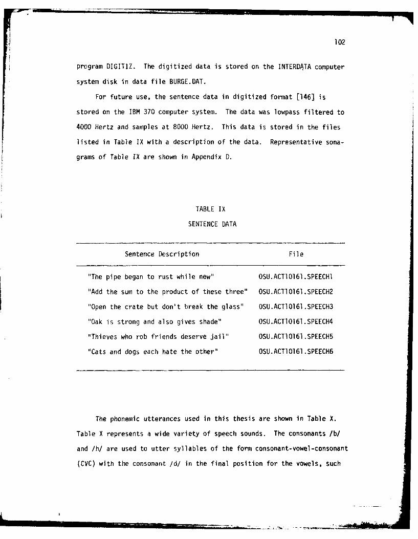
102
program DIGITIZ. The digitized data is stored on the INTERDATA computer
system disk in data file BURGE.DAT.
For future use, the sentence data in digitized format [146] is
stored on the IBM 370 computer system. The data was lowpass filtered to
4000 Hertz and samples at 8000 Hertz. This data is stored in the files
listed in Table IX with a description of the data. Representative sona-
grams of Table IX are shown in Appendix D.
TABLE IX
SENTENCE DATA
Sentence Description File
"The pipe began to rust while new" OSU.ACTIO161.SPEECHI
"Add the sum to the product of these three" OSU.ACT1O161.SPEECH2
"Open the crate but don't break the glass" OSU.ACT!0161.SPEECH3
"Oak is strong and also gives shade" OSU.ACT10161.SPEECH4
"Thieves who rob friends deserve jail" OSU.ACT10161.SPEECH5
"Cats and dogs each hate the other" OSU.ACT10161.SPEECH6
The phonemic utterances used in this thesis are shown in Table X.
Table X represents a wide variety of speech sounds. The consonants /b/
and /h/ are used to utter syllables of the form consonant-vowel-consonant
(CVC) with the consonant /d/ in the final position for the vowels, such

103
TABLE X
PHONEMIC DATA
No. Utterance No. Utterance No. Utterance No. Utterance
S -- 41 /y/ 81 /fl 121 /hid/2 /i/ 42 /y/ 82 /bit/ 122 /hld/3 /i/ 43 /m/ 83 /bIt/ 123 /hEd/4 /1/ 44 /m/ 84 /bct/ 124 /h ed/5 /I/ 45 /n/ 85 /baet/ 125 /hAd/6 /C/ 46 /n! 86 /bAt/ 126 /hTd/7 /c/ 47 /n/ 87 /hDt/ 127 /hUd/8 /W/ 48 /n! 88 /bUt/ 128 /hud/9 /av/ 49 /b/ 89 /fut/ 129 /h7d/
10 /A/ 50 /bI 90 /but 130 /hald/11 /A/ 51 /d/ 91 Ibl 131 lh:)Idl
12 /a/ 52 /d/ 92 /aIs/ 132 /haUd/13 /a/ 53 /g/ 93 /bDI/ 133 /hoUd/14 /D! 54 /g/ 94 /baU/ 134 /held/15 /DI 55 /p/ 95 /boU/ 135 /hjud/16 /U/ 56 /p/ 96 /belt/ 136 /awa/17 /U/ 57 /t/ 97 /Iju/ 137 /ala/18 /u/ 58 -- 98 /wIl/ 138 /ara/19 /u/ 59 /t/ 99 /111/ 139 /aya/20 /YY 60 /k/ 100 /rIlI/ 140 /ama/21 /?/ 61 /k/ 101 /yIl/ 141 /ana/22 /al/ 62 /h/ 102 /mIl/ 142 /serV23 -- 63 /h/ 103 /nilI 143 /aba/24 /al/ 64 /I 104 /sen/ 144 /ada/25 /I/ 65 /I 105 /bIl/ 145 /aga/26 /DI/ 66 /tf/ 106 /dIl/ 146 /apa/27 /aU/ 67 Itf/ 107 /gIl/ 147 /ata/28 /aU/ 68 /v/ 108 /pIl/ 148 /aka/29 /oU/ 69 /v/ 109 /tIl/ 149 /aha/30 /oU/ 70 /V/ 110 /kIl/ 150 /aja/31 /eI/ 71 // ill /hIl/ 151 /atfa/32 /eI/ 72 /z/ 112 /Ill/ 152 /ava/33 /jU/ 73 /z/ 113 /tfIl/ 153 /aga/34 /jU/ 74 /f/ 114 /vIi/ 154 /aza/35 /w/ 75 /f/ 115 / aet/ 155 /afa/36 /w/ 76 /e/ 116 /all/ 156 /aea/37 /1/ 77 /0/ 117 /fIl/ 157 /asa/38 /1/ 78 /s/ 118 /baO/ 158 /afa/39 /r/ 79 /s/ 119 /sIl/40 /r/ 80 If! 120 IfIl/

104
as /hid/. The vowel /a/ is used to utter nonsense syllables of the form
vowel-consonant-vowel (VCV) in both initial and final positions, such as
/aba/. A set of minimal units using the final form -/Il/ (-ill) is used
for the consonants also. Some of the other syllables used are English
words. The basic sounds are found in Table 11.
The phonemes are analyzed by the algorithms in Appendix B. The
energy data is shown in Table XI, normalized by the sound Ix/ for the
first 81 phonemes in Table X. The energy in the phoneme /ce/ corresponds
to the largest compared to each of the other phonemes. The data is cal-
culated by the program ENERGY. From Table XI, it can be seen that the
energy of the prediction residual divides the phonemes into classes by
phonemic aggregations.
It is well known that with simple LPC methods [60], the excitation
function is a set of periodic pulses or random noises which can be iden-
tified as high or low energy excitation functions. However, by using the
energy data in Table XI, the phonemes can be grouped into three classes,
namely high energy, low energy and noise groups. The high energy group
includes the vowels and diphthongs. The plosive, fricative and unvoiced
phonemes make up the noise group. The low energy group is composed of
glides and nasals. It follows that an ideal excitation signal for speech
would enhance perception by considering a three-tier classification
rather than the conventional two-source model. This would include a
source for vowels, a source for nasals and glides, and a source for
fricatives. This is the result of the phoneme energy study of the pre-
diction residual. A normalized energy distribution by phoneme for each
sub-band is shown along with the energy bands in Figure 24.
! i I

105
TABLE X!
ENERGY BY PHONEME FOR PREDICTION RESIDUAL
TotalPhoneme Frequency Band SBI SB2 SB3 SB4
/i/ .44 .58 .46 .33 .3i
/1/ .75 .51 .46 .75 .45
/E/ .84 .65 .47 1.0 .$4/c/ 1.00 1.00 1.00 1.0 1.00/A/ .72 .67 .57 .45 .41/a/ .72 .64 .69 .59 .35/D/ .83 .60 .68 .70 .42/U/ .24 .23 .25 .20 .15/u/ .19 .29 .10 .11 .20A/ .61 .62 .22 .64 .15
/aI/ 1.00 1.00 .79 .68 .65/DI/ .44 .75 .45 .20 .32
/aU/ 1.00 1.00 .95 .90 .78/oU/ .56 1.00 .31 .21 .53/eI/ .86 1.00 .64 .66 .49/jU/ .32 .67 .21 .22 .12/w/ .24 .35 .24 .10 .23/1/ .24 .29 .08 .10 .29/r/ .14 .24 .12 .09 .07/y/ .11 .20 .08 .08 .07/m/ .34 .65 .25 .22 .19/n/ .22 .45 .17 .18 .13n/ .37 .67 .37 .24 .18/b/ .24 .49 .11 .14 .17/d/ .32 .63 .27 .14 .21/g/ .31 .50 .18 .14 .16
/p/ .18 .27 .08 .07 .08
/t/ .45 .46 .32 .26 .25/k/ .32 .63 .23 .19 .20/h/ .45 .46 .24 .31 .31
/j/ .53 .51 .44 .31 .58
Itfl .23 .46 .16 .10 .11/v/ .16 .29 .13 .09 .09/1/ .17 .32 .13 .12 .10/z/ .24 .44 .17 .19 .15
/f/ .07 .04 .07 .05 .12
/e/ .11 .21 .09 .07 .05
/s/ .08 .05 .06 .06 .13WY .10 .06 .07 .07 .18

106
ENERGY DISTRIBUTION
1.00- 1
75-
w .50-
w HIG H
.25 -
.,.-LOW
NOISE01I
I 2 3 4
SUB-BAND nFigure 24. Normalized Energy Distribution by Sub-Band

107
Based on the above discussion, phonemes can be classified into three
energy groups: (1) high energy (HE), (2) low energy (LE) and (3) noise
(N). To do this, the normalized residual phoneme energies (second column
in Table XI) are the first tabulated; from this, there are clear breaks
in the energy levels and therefore three energy groups formed. These
breaks are used to identify the threshold values for a particular energy
group. For the high energy group, let T11 be the threshold value. That
is, any phoneme that has normalized residual energy greater than T11 is
classified into the high energy group. Similarly, T2 2 and T33 are the
established threshold values for low energy and noise phonemes respec-
tively. The three groupings are given in Table XII. The threshold
values Tii, i = 1, 2, 3, can be identified from Figure 24. These are
for the entire frequency range.
TABLE XII
PHONEME ENERGY GROUPINGS
Energy Groups Phonemes
HE i, I, , a , a, A, D, U, u,
LE m, n, n, z, w, 1, r, y
N f, f, b, d, g, p, t, k
I*

108
For the sub-band coding, threshold values need to be computed for
each band. Also, each energy group has to be divided into four subgroups
corresponding to the four sub-bands. Let Ein be the normalized signal
energy in the nth frequency band corresponding to the phoneme that is in
the ith energy group. This is explicitly shown in Table XIII. For
example, E12 represents the energy in the second frequency band corre-
sponding to the high energy phoneme (first energy group).
The threshold values for Ein (referred hereafter as Ein) in Table
XIII will now be established using columns 3, 4, 5 and 6 in Table XI.
TABLE XIII
SYMBOLIC REPRESENTATION OF ENERGY DISTRIBUTION
Frequency Band
1 2 3 4
H E11 E12 E13 E14
LE21 E22 E23 E24
U-j
N E31 E32 E33 E34
E. is listed for various phonemes in columns 3, 4, 5 and 6 inin
Table XI. To make the classification speaker independent, the Ein has
to be normalized by ET given in (3.24). Let
__ _

109
ET En n = 1, 2, 3E.i ETiin T n =1, 2, 3, 4 (3.25)
From this, it is clear that
T <=1,2,3Ein .0 n =l, 2, 3, 4 (3.26)
As before, ET in (3.25) are tabulated for i = 1, 2, 3 and n = 1, 2,in
3, 4. The breaks are established from this tabulation and the threshold
values are obtained from these breaks. These are tabulated in Table XIV.
The array in Table XIV will be referred hereafter as energy threshold
matrix. This matrix will be used in computing the bit allocation scheme,
which is discussed in the next chapter.
TABLE XIV
ENERGY THRESHOLD MATRIX
Frequency Band
1 2 3 4
H .58 .27 1.0 .75
L .50 .19 1.0 .86
N .46 .27 1.0 1.00
.

110
3.9 Sunuary
In this chapter, th.pr basis of coding the prediction residual at the
rate of 9600 bits/second using the techniques of sub-band coding was pre-
sented. Transform coding and sub-band coding wwere discussed along with
their relationship. The method of achieving maximum intelligibility
based on the Articulation Index was presented. Transitional information
of speech along with the relation of speech perception to intelligibility
was discussed. Phonemes have been divided into three energy groups so
that these can be used in the bit allocation scheme to be discussed in
Chapter IV.

CHAPTER IV
ENERGY BASED SUB-BAND CODING ALGORITHM
4.1 Introduction
In this chapter the sub-band coding algorithm, introduced in Chapter
III, is examined with the prediction residual as the input source signal.
The coding algorithm combines spectral analysis and waveform coding tech-
niques. The combination is intended to provide perceptual enhancement of
the speech. The perceptual aspects of speech are a key factor in the bit
distribution of the coding algorithm. The bit allocation is established
by using the energy groups discussed in the last chapter. For each frame
and for each sub-band, the energy En = IEfn(k)l 2 is computed, whereN k
En indicates the energy corresponding to the nth sub-band in a given
frame.
It is well known that most of the spectral density for vocalic
sounds and the fundamental frequency are basically found in the sub-band
number one (lowest frequency band). The intensity of the energy is sub-
stantially high. Spectrogram data can show this. The second formant
resides predominantly within the second and third sub-bands and is of the
low energy type. These formants determine the transitional cues for cer-
tain perceptual effects. The energy of noisy speech sounds, i.e., voice-
less fricatives, plosives, etc., has a basic flat spectrum and most of
the energy is above 2 kHz. The perceptual effects are discerned in this
frequency range. The spectrograms show the intensity of the signal
111

112
energy represented by varying shades of gray or black areas [2]. The
higher the energy, the darker the area. Spectrograms are included in
Appendix D. These figures are included to show the different energy
levels associated with different phonemes. From these spectrograms, it
can be seen that vowels are typified by dark areas; whereas fricatives,
plosives, etc., are shown in a gray area. Although all voiced sounds
show a dark color on the spectrogram, Makhoul and Wolf [90] have shown
that nasals and glides have a lighter shade when compared to other voiced
sounds.
In this study, the energy in each frame of the prediction residual
is calculated for each type of phoneme. The bits per sample in each band
is allocated on an adaptive basis, using the perceptual criteria dis-
cussed in the last chapter. The next section deals with the bit alloca-
tion scheme.
The bit allocation method is incorporated into the sub-band coder,
which is discussed in Section 4.3. The adaptive strategy is combined
with a uniform quantizer with results presented in Sections 4.4 and 4.5.
Section 4.6 gives the details of the modules for computational aspects
of the coding of the prediction residual.
4.2 Bit Allocation
In this section, the bit allocation scheme is discussed using the
energy groupings in Tables XII in Chapter III. In symbolic form, the bit
distribution is shown in Table XV for a three-energy level--four sub-band
coder, where the rows correspond to the energy levels and the columns
correspond to a particular frequency band. For example, k23 bits per23j

113
sample are assigned for the second energy (LE) band and the third fre-
quency band.
TABLE XV
SYMBOLIC REPRESENTATION OF BIT DISTRIBUTION
Frequency Band
1 2 3 4
High Energy (H) kll k12 k13 k14
Low Energy (L) k2 1 k2 2 k2 3 k24
Noise (N) k31 k32 k33 k3 4
The bits are allocated by the empirical formula
E.. i = 1, 2, 3k. . 1092(1 + 11
13j = 1, 2, 3, 4 (4.1)
where E.. is the energy from Table XIII and a. is a normalization factor
determined from the constraint
4E ki N. = C i = 1, 2, 3 (4.2)
j=l 13 3
with Nj, j 1, 2, 3, 4, being the number of samples in each band after
decimation. The value of C is equal to the total number of bits/frame

114
minus the number of sync bits per frame. Combining (4.1) and (4.2), it
follows that
4 E..
j=l Nj[1og2 (l + 1'-)] = C i = 1, 2, 3 (4.3)
where the normalization factor, aj, can be determined from (4.3). Equa-
tions (4.1), (4.2) and (4.3) define the algorithm.
The normalization factor is included to take into consideration the
perceptual aspects of the signal. It is used as a weighting factor for
transitional cueing. It has been shown that pitch, formant areas, nasal-
ity and affrication are important for speech perception. Within the
speech spectrum, these characteristics occur in certain frequency ranges.
The power density of speech can indicate this conception, and is dis-
cussed below.
The speech power density spectrum is shown in Figure 25. It is
clear that most of the energy is below 1000 Hertz. It has been shown by
Miller and Nicely [91] that below 1000 Hz, voicing, nasality, and affri-
cation are predominant for determination of the phonemic content. It has
been pointed out that given a set of speech signals, a weight factor can
be derived when the speech is separated into sub-bands. When these sig-
nals are coded properly, there is an advantage of distinguishing certain
perceptual effects such as voicing, nasality and affrication. The per-
ceptual effects can be used for calculation of bits for coding.
To compute the normalization factor properly for coding the residual
signal, a bit matrix is chosen. The bit distribution that is selected is
based on perceptual concepts. This matrix will be referred to as an a
priori hit matrix. In addition to perceptual concepts, the a priori bit

115
15
12
cn9z
w 6
0
3-
0 1 2 3 4 5FREQUENCY IN KHz
Figure 25. Power Density of Speech Signal (After Noll, 1975)

116
matrix is selected such that the bit rate is 9600 bits/second for the
sub-bands given in Table IV. The matrix is shown in Table XVI, where the
Aentries will be referred to as k. to denote the a priori values.13_ ____
TABLE XVI
A PRIORI BIT MATRIX DISTRIBUTION
Frequency Band
1 2 3 4
High Energy 1 4 3 2 2
Low Energy 2 3 3 3 2
Noise 3 2 3 3 3
The a priori bit matrix is based on experimental results on pho-
nemes. A cursory inspection of Table XVI reveals that the perceptual
criteria is preserved. For example, on lower bands where pitch and for-
mant data must be preserved as accurately as possible, a large number of
bits per sample are used for encoding, whereas for upper bands where
fricatives and noisy sounds are predominant, fewer bits per sample are
used. Note that the same number of bits for each energy group is allo-A
cated. Also, the a priori bit values (k. ) are used to compute the nor-
malization factor in (4.1).
Id

I'7
117
When the energy of the speech sound is determined to be high enough,
the energy threshold introduced in Chapter III selects the energy matrix
(from Table XIII) and a priori bit values (from Table XVI). These are
used to calculate the normalization factor from (4.1), and
ET i = 1, 2, 3_ ij (4.4)
-J (k A ) A 1 = 1, 2, 3, 4
T
where Ei is the energy obtained from threshold matrix and kA. is obtained
from the a priori bit matrix. Figure 26 gives the distribution of (1/aj)
based upon (4.4).
Equation (4.1) can mow be used to allocate the bits. It should be
pointed out that in using this equation, actual energy values of the sig-
nal will be used rather than the threshold values. The following steps
are performed to allocate the bits.
1. Spectral estimates are computed for each sub-band.
2. The total energy in the frame for the entire frequency band is
computed.
3. Eij's are computed.
4. Normalization factor, oj, is computed
5. The bits are allocated by
E.l i = 1, 2, 3k ij = 10g2 (l + o0-o1j) (4.5)1j =1, 2, 3, 4
where E.. is the energy in the jth sub-band corresponding to the ith
energy group and o. is the normalization factor from (4.4). Figure 27
gives the flow chart for the bit allocation scheme.

118
DISTRIBUTION OF
4.0-
3.0-
2.0 !' \ NOISE
0---c
1.0 "
LOW ~$IH IGH
0 I
1 2 3 4
SUB-BAND jFigure 26. Distribution of Normalization Factor

119
BIT ALLOCATIONBY SUBBAND
'ef (n)
SPECTRAL
ESTIMATE
SUBBAND NORMALIZATIONENERGYCONSTANT { O-1ESTIMATEESTIMATE
BITALLOCAT ION
BITS l og, (I+ allj
Figure 27. Flow Chart for Bit Allocation

120
Equation (4.5) has been simulated using the phonemes in Table XII.
The bits are averaged for each energy group. The results of the simula-
tions are shown in Figure 28 for each of the three energy groups. Dis-
tinctly shown is a separation of the energy groups. Note that the low
energy group which contains the nasalic and glide sounds is shown to
separate the high energy and noise groups. This separation supports the
three-source theory of the residual signal.
Earlier, it was shown that the residual signal parallels glottal
excitation. The use of the residual signal for encoding the speech and
later exciting the speech synthesizer has several benefits. The bits are
minimized in the first and second sub-bands, reducing the necessary trans-
mission rate for these sub-bands. It is unnecessary to transmit twice as
many bits for sounds with nasalic, glide or liquid characteristics. On
the other hand, the discrimination from the noise is shown to be distinct.
The benefit remains clear further, because perceptual criteria will be
enhanced in all sub-bands. Discrimination of sounds can be benefited with
a minimum bit allocation.
The bit distribution is shown by frame for each phoneme in Figure 29.
Again, it is shown that the perceptual criteria is preserved in that the
pitch and formant prediminant phonemes receiving a substantial bit allo-
cation and fewer bits are allocated for fricative and plosive phonemes.
Noting that the total number of allowed bits per frame is constant, the
difference in bits per energy group is adjusted in the synthesis bits.
This is discussed in detail in the next section.
4.3 Sub-Band Encoding of the Prediction Residual
The bit allocation scheme was used in the perceptual aspects of

121
BIT DISTRIBUTION BY SUB-BAND
5
4-
3-
_\- HIGH
to 2-LOWN
0NOISE
0 1 I
1 2 3 4
SUB-BAND nFiqure 28. Bit Distribution for Sub-Bands by Energy Bands

122
speech in sub-band coding of the prediction residual. The sub-band coder
partitions the frequency band of the residual signal into four sub-bands
by using the bandpass filters. The partitioning of the frequency bands
is shown in Figure 20. Each sub-band is low-pass translated, decimated
[by the Nyquist interval obtained from (3.15)], and encoded according to
the bit allocation scheme discussed above. It has been shown that sepa-
rate coding of each sub-band accomplished the preferenctial perception
criteria for that band [37]. The decoding of each sub-band involves an
interpolation and translation back to the original band. The bands are
summed to arrive at an estimate of the original residual signal (see Fig-
ure 21). This section describes the sub-band coding parameters, the
relation of the sub-bands to the Articulation Index and other perceptual
criteria discussed in this thesis.
The cutoff frequencies for the sub-band coder are shown in Table
XVII. The guideline established for selection of cutoff frequencies is
to represent an approximately equal contribution to the Articulation In-
dex. The bands shown in Table XVII represent enough of the important
frequencies such that intelligibility is preserved.
TABLE XVII
SUB-BAND CODER CUTOFF FREQUENCIES
Band Cutoff Frequency (Hz)
1 250 - 5002 500 - 10003 1000 - 17004 2000 - 3000

123
BIT DISTRIBUTION BY FRAME
15
w 10000 X0 0
4 0
00
0 0
0 00I It0 110 12100 1010 1010 10
I CaeQA :uuirmnr)zwr ys fbd'gpt k
"E (VOCALIC) LE (NASAL, GLI DE) NC RI CATI yE)
PHONEMEFigure 29. Bit Distribution for Phonemes by Frame

124
The integer-band sampling scheme [37] was also analyzed at the sam-
pling rate of 8000 Hertz. The technique requires the ratio of upper to
lower cutoff frequencies of the sub-band be (mi + 1)/m i, where mi is an
integer. These bands are related at the bit rate such that the data can
be synchronized when multiplexed. Table XVIII is helpful in constructing
the sub-bands. Previous authors have given the choice of bands that re-
late at other sampling rates [36] [37]. Shown in Table XVIII are integer-
band sampling cutoff frequencies for an 8000 Hertz sampling rate. The
integer decimation ratio is shown in Column 1 for 8000 Hertz. The band-
widths, ft are indicated in Column 2. The sampling rate, 2fi, is shown
in Column 3. In Columns 2, 3 and 4, the cutoff frequencies are indicated
implicitly. Integer-band sampling is not used in this thesis, and is
given here for completeness.
To explain how each band is related, the analysis of the sub-band
coder is discussed. The sub-band coder is designed for 9600 bits/second.
The transmitted coder parameters include the sub-band coded prediction
residual signal, PARCOR coefficients and sync bits. Table XIX represents
a breakdown of sub-band coder parameters for the high energy phonemes.
Table XX shown sub-band coder parameters relative to the low energy
sounds. Table XXI represents those parameters relative to the noise
sounds. The difference in Tables XIX, XX, and XXI are the bits allocated
and the transmission rates per band, and the sync bits.
It is well known that the decimation rate shown in Column 4 of Tables
XIX through XXI represent an integer number of samples available before
encoding. These available samples are related to the 9600 bits/second
transmission rate. The fractional representation for each frame and sub-
band samples are shown in Table XXII.

125
TABLE XVIII
INTEGER-BAND SAMPLING CUTOFF FREQUENCIES FOR8000 HERTZ SAMPLING RATE
Decimation f 2fi 3fi 4fiRatio 1 1 1 1
1 4000 8000 12000 160002 2000 4000 6000 80003 1333 2666 3999 53324 1000 2000 3000 40005 800 1600 2400 32006 666 1332 1998 26647 571 1142 1713 22848 500 1000 1500 20009 444 888 1332 1776
10 400 800 1200 160011 363 728 1089 145212 333 666 999 133213 308 616 924 123214 286 572 858 114415 266 534 798 106416 250 500 750 100017 235 470 705 94018 222 444 666 88819 210 420 630 84020 200 400 600 80021 190 380 570 76022 182 364 546 72823 174 348 522 69624 167 334 501 66825 160 320 480 64026 154 308 462 61627 148 296 444 59228 143 286 429 57230 133 266 399 53231 129 258 387 51632 125 250 375 500

126
a
4.) 4 D
iEI0 0 0 a~ 0 Q~~0-
LikL
wI-
aga
La
~U4
LL.
C-- Wn (
0 C
I.I.
U
LU 0 1 -J* n 8% 9-
CMI Sn IScm CA
4Jo-~ 0 0C'
u-(%S.- ~ U
cj tn0
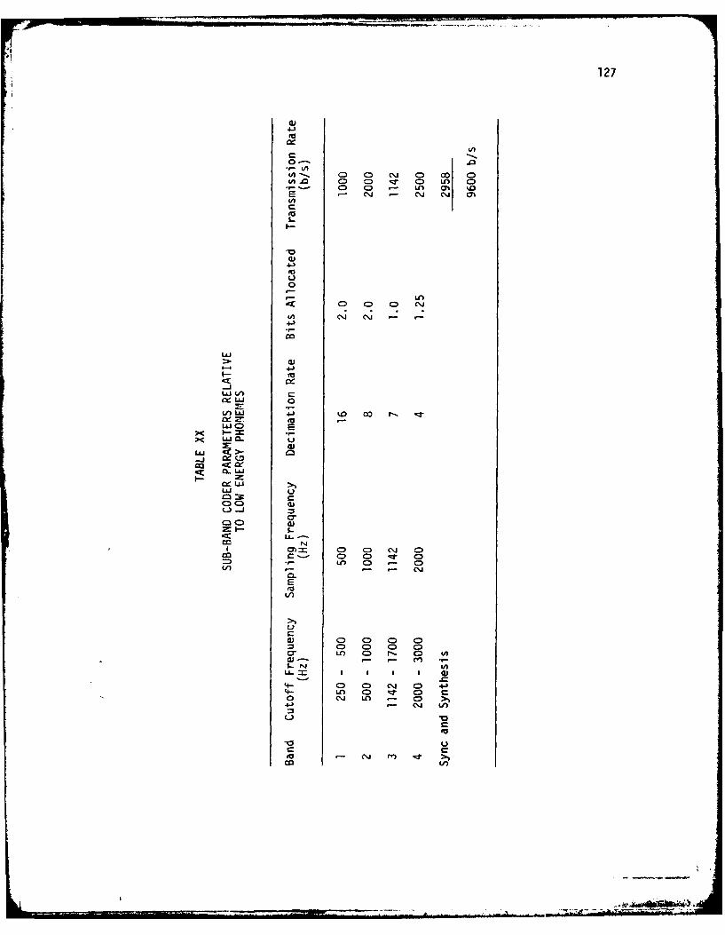
127
4J)
0-.
u-D. 0 C0 C~J 0o 00 0D*.-. 0 D 0 r - LA C L
E - CJ - C\j C\J
LL
4-)
0
ac LA
ui a
0JJ CD
EDco C) ~ CD r C
LAJO E
)( .--
CC
6-
4- 0 0 C 0 4-4- O -C .4 CE
0 A.L4- E .mU
En >
cm,

128
4A
%0 O
*9--
I-I
4-
Go
41,
6A 2: 60 00 10. .d
4JJ
CL =
c CD C w
4J -
4- LCa~f C ~ f4-jDl

129
TABLE XXII
REPRESENTATION OF SAMPLES FOR A FRAME FOR HIGH ENERGY SOUND
Band Fraction/Frame Samples/Frame
1 .207 53
2 .312 80
3 .180 45
4 .207 53
Sync and Synthesis .094 24
1.000 256 Samples/Frame
The multiplexing (see Figure 21) is simulated on the computer by
first appending each of the decimated signals to 256 points per frame by
adding zeros. Second, the DFT's of these are taken. Third, the trans-
formed signals are summed. Finally, the IDFT of the summed signal is
the multiplexed signal, which has 256 points. The demultiplexing in
Figure 21 is simulated using the inverse process. That is, first, the
decoded signal is transformed. Second, it is divided into four frequency
bands. Third, these frequency coefficients in each band are appended by
zeros to get 256 points. Finally, the IDFT of these signals are taken,
which gives the demultiplexed signals.
Shown in each of Tables XIX through XXII is a band labeled "Sync and
Synthesis." These parameters include synchronization bits and synthesis
parameters for the receiver. The synchronization bits include one to

130
establish the beginning of a frame and three to determine if the frame
contains a high, low or noise energy signal. The remaining samples in
the sync and synthesis bits are allocated to the PARCOR coefficients for
synthesizing the speech.
The PARCOR coefficients are distributed between the range of IkjI <
I and, in most cases, the entire range is not required [28]. It has been
shown that the odd-ordered coefficients are somewhat skewed toward the
positive side, whereas the even-ordered coefficients are someqhat skewed
toward the negative side [28]. The limitation of a quantizer range re-
sults in better speech quality for a given number of bits assigned to
each coefficient. These parameters have been studied in depth in the
literature. Further quantization characteristics of the PARCOR coeffi-
cients can be found in [7) [28] [31] [119]. Thse aspects are used in
adjusting the synthesis bits in Tables XIX to XXII, and is outlined
below.
Specifically, the following procedure can be used in assigning bits
for synthesis parameters. For high energy sounds, 20 bits can be utilized
for the 10 PARCOR coefficients. The bit allocation for low energy sounds
for the PARCOR coefficients is 70. For the noise energy sounds, the bit
allocation is 170. Note that more bits are available for the PARCOR
coefficients corresponding to the low energy and the noise signals as
compared to the high energy signals. These allocations in synthesis
parameters for encoding are adequate. Actual implementation of the bit
allocations for the PARCOR coefficients and their effect on the coder has
yet to be done.
The find tuning of quantization parameters has yet to be done. The
total sub-band system requires many trade-offs in the analysis section.

131
In the analysis section, allowance must be made for the transmission rate
for each sub-band. In the next section, the uniform quantization method
is discussed.
4.4 Adaptive Uniform Quantization
The sub-band coder partitions the residual signal into four fre-
quency bands. These banded signals are passed to the quantizer for re-
duction of information content. The design of the quantizer is determined
by the bits allocated as discussed earlier. The amplitude of each resid-
ual signal sample is quantized into one of 2IBITS levels, where IBITS is
the number of bits allocated for the sub-band. The information content
of the digitized signal is IBITS bits per sample. It is shown in Column
6 in Tables XIX through XXI that the information rate for each sub-band is
Information Rate = (Sampling Freq.)n x I bits/second
I = l, ..., IBITS (4.6)
where (Sampling Freq.)n is the sampling frequency for the nth sub-band.
After quantization the discrete amplitude level of the signal sample
has a value expressed in binary decimal of length IBITS. The value of
IBITS ranges from I to 5. For example, the value of 2 for IBITS yields
amplitude levels of 00, 01, 10 and 11; whereas, a value of 5 would yield
32 five binary length words.
The range of the quantizer is aligned such that the amplitudes of the
input residual signal will be within the range of the maximum swing of the
output of the quantization levels. The methcl for accomplishing the
assurance that no overload occurs is based on a scheme of analyzing each
frame before quantization; i.e., the range of the signal is found before
quantization. This is compared to the bits allocated. An adjustment is

132
made if needed by rounding the bits allocated to the next integer. The
method of quantization will be discussed next. 4
It has been shown that a characteristic of sub-band coded speech is
that it has no sample-to-sample correlation [36] [37]. Following this,
encoding is best performed by adaptive pulse code modulation (APCM) [109]
(121). Previous encoding based on differential or fixed prediction does
not achieve good results for speech using sub-band coders [37]. Each
sub-band utilizes a uniform quantizer characteristic. Each sub-band
exhibits a different level of energy; therefore, an adaptive uniform
quantizer is used utilizing a technique that shrinks and expands the
quantizer by sub-band such that the signal is within the range of the
maximum quantization level for that sub-band.
To implement the adaptive uniform quantizer, let the step size be
denoted by A. Figure 30 illustrates the characteristic for the adaptive
uniform quantizer [109] and will be idscussed in detail. It is well
known that the uniform quantizer level produces error which follows the
uniform distribution. That is, the probability density function of the
quantization error Qe is given by
f = A <Qe < 2 (4.7)
with the variance
(72(Qe A2 (4.8)
The step size is dependent on the bits allocated.
Let the number of levels be represented by
NL = 2i i = 1, ... , IBITS (4.9)

133
OUTPUT Qi
-a&aINPUT (k)-C. A*-A -3a -2a 0 a 2 3A..k AMPLITUDEef
Figure 30. Characteristic of the Adaptive Uniform Quantizer

134
then
Aefn(n) ] (4.10)A-NL fn max
where e fnn ]max is the maximum value of the nth sub-band residual
signal.
In order to achieve the quantized value, let
j = [&l' &2 .... , NL (4.11)
be an MyL)-vector used to identify the parameters of the quantizer levels
such that
Q = A• (4.12)
where the vectors _Q and _ are of dimension NL and represent the quantizer
values. The entries in 9 are given by
(LK(L 2- k + I) 1 < < N
2 - 2
0 NL
NL+ 2 < R < NL (4.13)
2 _
From (4.12) and (4.13), it follows that the quantized level Q in Q is
given by
Q t = A •(4.14)
The quantized values of the residual signal are obtained by rounding it
to the nearest quantized level, which is used to code the signal.
In the next section, performance measures are discussed for the
quantizer and the sub-band coder.

135
4.5 Signal-to-Noise Ratio
Performance Measurements
In the previous section, the quantization is done for the banded
prediction residual. In this section, performance measuremetns will be
discussed. It has been recognized in the literature that signal-to-noise
ratio (SNR) is an inadequate performance measure for speech coding [109].
This idadequacy is realted to the idea that additive white noise is not a
good model for error waveforms in speech quantization. Generally, most
authors supplement the SNR by subjective and perceptual measurements as a
rule.
The SNR is still the single most informative measure for quantizer
performance (109]. If the quantizer is designed for maximum SNR, the
step size can be chosen according to the probability density function of
the signal [122]. However, the SNR improvement is offset by greater idle
channel noise for speech [123]. The result is poorer subjective perfor-
mance [123]. Therefore, to enhance SNR an adaptive quantizing technique
is used based on the allocation of bits.
It has been shown that transform coding with adaptive quantizers
maximizes SNR and lowers the idle channel noise [81]. Intuitively, sub-
band coding should follow under similar conditions. With sub-band
coding, the quantization noise of each band is contained within that band
and therefore, minimizes the quantization noise of the coded speech [36].
Due to the characteristics of the speech spectrum, the quantization dis-
tortion is not equally detectable at all frequencies. This technique
offers a means of controlling the quantization noise across the speech
spectrum and, therefor a realization of improvement in signal quality
[36).

136
The definition of each objective measure will be discussed next.
Perhaps the most common measurement of performance is the conventional
(normalized) SNR which is defined as
N-i 1(x(k) -y(k))
NSNR = -10 logo N-I (4.15)
E x2(k)k=OJ
where x(k) is the input to the coder and y(k) is the output of the de-
coder. It is assumed that the numerator represents the noise of the
coding technique, such that as the noise decreases a smaller SNR will be
the result of the summation in (4.15). The advantage of this quantity
is a representation of the normalization of the error between the coder
input and the decoder output. For speech there is no perceptual advan-
tage in maximizing the SNR; however, the SNR in (4.15) could be optimized
for the autocorrelation of the speech [122].
Another measure similar to (4.15) is the root-mean-square error
which is defined as
E (x(n) - y(n) )2
RMSSNR = -20 log,,o n=O N (4.16)
where x(n) and y(n) are defined as before. In (4.16), the error is
assumed to be of random nature, and is normalized by the factor N, the
number of data points.
A third measure is defined as
-- ~V 4 ..

137
1N- 1 [(x(n) - y(n) 2
MSSNR = 10 log (4.17)n=O I 2n
where x(n) and y(n) are expressed as before. The representation in (4.17)
defines some measure of error.
The results using (4.15), (4.16) and (4.17) are shown in Table XXIII.
These are computed by program SNRCAL (see Appendix B). These results
exemplify good coder performance. Note that these simulations are done
without bit assignment to PARCOR coefficients. Several phonemes are used
in these measurements and they give an adequate measure of the coder.
However, the complete simulation should include quantization of all param-
eters to complete the 9600 bits/second coding algorithm. The next section
discusses the computational aspects for coding and decoding the prediction
residual.
TABLE XXIII
SIGNAL-TO-NOISE PERFORMANCE MEASUREMENTFOR SEVERAL PHONEMES
Phoneme RMSSNR NSNR MSSNR
/1/ 29.2 36.7 18.2/e/ 37.2 36.9 19.1
/ae/ 35.1 37.4 17.5/A/ 32.9 34.9 15.2/a/ 30.1 38.4 18.3/u/ 36.8 38.7 17.7/1,4 29.8 38.0 18.4
/al/ 31.3 37.0 18.2/aU/ 34.2 38.4 18.7/oU/ 29.4 37.9 16.8/el/ 33.4 39.0 17.0

138
4.6 Comiputation for Coding the
Prediction Residual
The flow chart that gives all the computer modules is given in Fig-
ure 31 for coding the residual signal. The data blocks shown in Table
XXIV represent data processed and online storage during the computations.
TABLE XXIV
DATA BLOCKS FOR PROCESSING AND STORAGE
Data Block Record Number ofName Length Records Module Used
BURGE.OAT 256 82 DIGITIZ/WINDOW
WINOOW.DAT 256 16 W4INDOW'JAUTO/LATTIC/INVERS
AUTO.DAT 176 16 AUTO/LATTIC/INVERS
RESIDUAL.DAT 256 16 INVERS/LATTIC/FFT!4GR/SUMLPD
SPECTM. DAT 256 16 FFTMGR/RESULT/(PITCH)
BITS.OAT 16 16 FFTMGR/SUMLPD/ENCODE
PHAZ.DAT 256 16 FFTMGR/RESULT
CODE.DAT 256 16 ENCODE/DECODE
SIGNAL.DAT 256 16 DECODE/RESULT
SQNR.DAT 256 16 RESULT
SBAND1.DAT 256 16 SUMLPD/ENCODE
SBAND2.DAT 256 16 SUMLPD/ENCODE
SBAND3.DAT 256 16 SUMLPD/ENCODE
SBAND4.DAT 256 16 SUMLPD/ENCODE

139
-JL
c-r
U) ,oLvt
LLJu
zz00
LJ
0. -- 0
0 - o< H LL
3C '3
0 b-
zg
I- 08 nu
Ili W4
La o 0o zo
__)__\___)_
-CD w

140
The modules are arranged to generate and use the data in Table XXIV
on the INTERDATA 70. The tape recorder inputs an analog signal to the
computer while DIGITIZ computes a sampled signal and stores the digitized
signal on disk in location BURGE.DAT. DIGITIZ is set up to store 4096
points. This program calls an assembly language digitizer and sequence
clock for sampling. This program is flexible for sampling any analog
signal and storing the signal on disk.
Program WINDOW uses the data on disk, BURGE.DAT. The data is win-
dowed using a 256-point Hamming window. The user has the option of
selecting which record of the digitized data to window. The program
reports the sequence selected and also scales the data. The window data
is written in data block WINDOW.DAT.
Routine AUTO calculates predictor and PARCOR coefficients using
Levinson's method [61]. The program uses as input the window data, WIN-
DOW.DAT. The output is an array, AUTO.DAT, containing autocorrelation
coefficients, predictor coefficients, cross-correlation coefficients and
reflection coefficients.
Routine INVERS uses the data from AUTO, AUTO.DAT, for use in the
lattice filter implementation from Equation (2.31) and (2.34). The order
of the filter is ten. The output from this program are the residual
values. This output is stored in RESIDUAL.DAT. Routine LATTIC is the
sames as INVERS except that LATTIC gives the user the option to produce
a plot of the speech and prediction residual on CALCOMP.
The FFTMGR module is an FFT manager that includes a bit reversal and
unscrambler. The input to this program is the prediction residual, RE-
SIDUAL.DAT. This routine calculates the avergae spectrum, magnitude
square and the energy of the prediction residual. It calculates the

141
energy per sub-band. It uses an a priori estimate of the energy and bits
to calculate the normalization factor and bits for each sub-band. The
program writes on disk the spectrum, SPECTM.DAT, the bits allocated,
BITS.DAT and the phase, PHAZ.DAT. It also gives the user the option for
a plot of the spectrum on CALCOMP.
Routine SUMLPD passes the prediction residual through a digital
bandpass filter. The signal is modulated, lowpass filtered and decimated
as shown in Figure 21. The input to this program is the data file RESID-
UAL.DAT. The outputs are the four sub-bands, SBAND1.DAT, SBAND2.DAT,
SBAND3.DAT, and SBAND4.DAT.
The signal corresponding to the four sub-bands are encoded using the
bits allocated in BITS.DATA by useing the program ENCODE. ENCODE allows
for 32 levels of code. In case of non-integer numbers, the quantizer,
QUNTIZ, rounds the bits to determine the number of quantizable levels.
A uniform quantization is used to determine the code. The output is
written in CODE.DAT.
Routine DECODE uses CODE.DAT as input. In the initial frame, the
maximum number of quantization levels is determined. This maximum sets
the level for the inverse quantizer. Then the signal is decoded and
written in file SIGNAL.DAT.
The program RESULT interpolates, modulates and bandpasses the signal,
SIGNAL.DAT, for reconstruction. The routine calculates signal-to-noise
ratio given by (4.15) and (4.17).
4.7 Summary
In this chapter, the energy based sub-band coding algorithm was pre-
sented. The method of allocation of bits was discussed. The design of
-* - -~

142
the sub-band encoding of the prediction residual was presented. The com-
putational aspects for coding the prediction residual were discussed.

CHAPTER V
SUMMARY AND SUGGESTIONS FOR FURTHER STUDY
5.1 Summary
This thesis investigates an efficient coding of the prediction resid-
ual using the technique of sub-band coding at the bit rate of 9600 bits/
second. The energy of the prediction residual is used to distribute the
bit allocation by sub-bands such that perceptual criteria is preserved.
The perceptual criteria is enhanced by transition information embedded in
the phoneme connections of speech by a technique that weights the energy
based on a normalization factor.
Each sub-band is partitioned such that there is an equitable contri-
bution to the Articulation Index as it is a measure of speech intelligi-
bility. This is discussed in relation to the quality of speech. The
perception of speech is described in a qualitative sense. The relation-
ship between the Articulation Index and transitional information is de-
scribed as a method of discrimination of speech sounds.
The prediction residual is discussed as ; parallel to the glottal
waveform. The prediction residual is formed by speech through an inverse
filter. This is represented as a deconvolution of speech from the vocal
tract filter.
The vocal tract filter is modeled as a recursive digital filter
using the method of linear prediction. Linear prediction produces the
143

144
prediction residual, which is the difference between the actual and pre-
dicted speech signals. Because the prediction residual is parallel to
glottal excitation, the prediction residual is an ideal pitch extractor.
A novel pitch extraction technique is presented. It is a two-stage
method that estimates the residual spectrum and uses time samples of the
residual to calculate the approximation of the pitch. The technique cal-
culates a threshold which uses squared samples to extract the pitch with-
in a frame. Also it includes an error check that estimates wide variances
of the pitch within each period and is then updated.
The three-tier classification of phonemes is derived from the energy
study of the phonemes for the prediction residual. It is shown that the
energy of the prediction residual divides the phonemes into classes by
phonemic aggregations, namely high energy, low energy and noise groups.
The high energy group includes the vowels and diphthongs. The plosive,
fricative and unvoiced phonemes compose the noise group. The low energy
group is composed of glides and nasals.
The three-tier classification of the energy levels along with the
four frequency bands allows for efficient allocation of bits per sample
for each band. The above method aids in preserving perceptual criteria
and preserves pitch-formant data by the allocation of a large number of
bits per sample in the lower bands. Since fricative and noisy sounds are
predominant in the upper bands, a smaller number is used in the lower
bands. The perceptual criteria is further enhanced by a normalization
factor.
The normalization factor is perceptual in nature and is used as a
weighting factor for transitional cueing. The derivation of the
145
normalization factor is discussed. Additional variations are given for
the relationship of the three phonemic classes to the normalization
factor.
The sub-band coder is designed based on the normalization factor,
the energy data, and the bit allocation. The parameters are computed on
a frame-by-frame basis. The sub-bands are constructed such that the bit
rate of the data from each band can be synchronized when multiplexed at
9600 bits/second. The integer-band sampling scheme is analyzed at the
sampling rate of 8000 Hertz for a 9600 bits/second transmission rate.
The sub-band coder is designed to transmit the coded prediction residual
signal, synthesis parameters and sync bits at the 9600 bits/second rate.
An integral part of the sub-band coder is the quantizer. The en-
coding of the signal is designed based on adaptive pulse code modulation.
Uniform quantization is used. The characteristics of the quantizer are
discussed in detail. Performance of the quantizer is described in terms
of signal-to-noise ratios (SNR) for objective criterion for quality. The
conventional (normalized) SNR is used for representing the error of the
coder input and the decoder output. The mean-square SNR is used for an
indication of gross error. These SNR measurements are only an indication
for quantizer performance. Generally, the SNR must be supplemented by
subjective and perceptual measurement as a rule. However, the SNR mea-
surements in this thesis are used without listeners.
In the following, some extensions to the present effort are sug-
gested. Appropriate references are indicated.

146
5.2 Suggestions for Further Study
5.2.1 PARCOR Coefficient Study of Sensitivity
The PARCOR coefficients introduced in Chapter II have been thoroughly
investigated because of their importance to speech analysis and synthesis
[9] [28] [31]. The priority is geared toward the synthesis of speech; in
that given the prediction residual and PARCOR coefficients, the speech
signal can be adequately regenerated. An extension of the present work
would enhance present efforts in this area by studying the sensitivity of
PARCOR coefficients with respect to the sub-band coding of the prediction
residual.
5.2.2 Sub-Band Coding Using Subjective
Measurements
The present work can be further advanced by the use of sub-band cod-
ing the prediction residual at various bit rates. The synthesized signal
would then be used in a comparative study for various bit rates. The per-
ceptual question concerning the method should be geared towards a record-
ing of the synthesized speech so that a set of listeners could hear the
results.
5.2.3 Energy Threshold Matrix Study
The introduction of the energy threshold matrix (ETM) in Chapter III
requires further study. In this work it is seen that the ETM is highly
dependent of perceptual criteria; consequently, several variations would
benefit the present work. In some instances, it is necessary to bias the
energy group to enhance the perceptual aspects; but this is unknown until

147
the energy distribution is computed. The results of ETM are dependent on
transmission rates; however, given one transmission rate, several ETM may
be equally applicable to the coding.
5.2.4 Integer-Band Coding of the Prediction
Residual
The integer-band coding method introduced in Chapter IV for use with
the prediction residual has not been considered in this thesis. It is
simple to implement and would minimize the need for modulators. Previous
authors have studied this for speech; however, the subject has not been
studied for the prediction residual [36] [37].
5.2.5 Prediction Residual and Noise
A study that would greatly benefit the speech coding area is to mask
the prediction residual with white noise. That is,
z(k) = ef(k) + v(k)
where ef(k) represents the discrete samples of the prediction residual
signal and v(k) represents the discrete damples of the white noise.
The enhancement of the pitch period markings would be of major impor-
tance in this study. Further, the synthesized signal-to-noise ratio per-
formance measurements would also be of interest. The speech waveform has
been examined in noise stripping environments; however, the prediction
residual in a noise environment has results that are promising [19] [58].
An aid to characterization of the signal would be to use the Laplacian or
Gamma distribution, as with the speech. However, these distributions are
questionable for the prediction residual since the waveform is different.
i . ... .. . - 4

148
Determining the probability distribution of the prediction residual may
be a study in itself.
5.2.6 Modeling the Prediction Residual
The prediction residual in this thesis is obtained by inverse filter-
ing the speech signal. Under certain conditions, it is not easy to code
the inverse filter; however, if a model was determined that is similar to
the signal, it would be of benefit for synthesis. An extension of the
work in Chapter II would be to compare the speech and the prediction
residual. It would be necessary to identify the essential parameters
that can be derived from the residual signal, such as pitch, phase in fo0
formant characteristic and noise between pitch period pulses. The end
results would approximate an expression that compares with the actual
residual pulse. This in turn could be compared with Flanagan and Rosen-
berg's work [2] [12] [32].

BIBLIOGRAPHY
(1) Delattre, P. C., A. M. Liberman, and F. S. Cooper. "Acoustic Lociand Transitional Cues for Consonants." The Journal of theAcoustical Society of America, Vol. 27, No. 4 (1955), 769-773.
(2) Flanagan, J. L. Speech Analysis Synthesis and Perception. New York:Springer-Verlag, 1972.
(3) Dudley, H. "Remaking Speech." The Journal of the Acoustical Societyof America, Vol. 11 (1939), 165.
(4) Dudley, H., R. R. Riesz, and S. S. A. Watkins. "A Synthetic Speak-er." Journal of the Franklin Institute, Vol. 227, No. 6 (1939),739-764-.
(5) Atal, B. S., and S. L. Hanauer. "Speech Analysis and Synthesis byLinear Prediction of the Speech Wave." The Journal of theAcoustical Society of America, Vol. 50, No. 2 Part -T (1971),
W3-16_55.
(6) Atal, B. S., and M. R. Schroeder. "Adaptive Predictive Coding ofSpeech Signals." Bell System Technical Journal (1970), 1973-1990.
(7) Markel, J. D., and A. H. Gray, Jr. Linear Prediction of Speech.New York: Springer-Verlag, 1976.
(8) Markel, J. D. "Digital Inverse Filtering - A New Tool for FormantTrajectory Estimation." IEEE Transactions on Audio and Elec-troacoustics, Vol. AU-20, No. 2 (1972), 129--37.
(9) Itakura, F., and S. Saito. "A Statistical Method for Estimation ofSpeech Spectral Density and Formant Frequencies." Electronicsand Communications in Japan, Vol 53-A, No. I (1970),T6-743.
(10) Un, C. K., and D. T. Magill. "The Residual-Excited Linear PredictionVocoder with Transmission Rate Below 9.6 Kbits/s." IEEE Trans-actions on Communications, Vol. COM-23, No. 12 (l975JT46----
1474.
(11) Markel, J. D., A. H. Gray, Jr., and H. Wakita. "Linear Prediction ofSpeech - Theory and Practice." Santa Barbara, California:Speech Communications Research Laboratory, Inc., SCRL MonographNo. 10, 1973.
149

150
(12) Rosenberg, A. E. "Effect of Glottal Pulse Shape on the Quality ofNatural Vowels." The Journal of the Acoustical Society ofAmerica, Vol. 49, No. 2, Part 2 (1971), 583-590.
(13) Dunn, J. G. "An Experimental 9600-Bits/s Voice Digitizer EmployingAdaptive Prediction." IEEE Transactions on Communication Tech-nology, Vol. COM-19, No. 6 (1971), 1021-1032.
(14) Gibson, J. D., S. K. Jones, and J. L. Melsa. "Sequential AdaptivePrediction and Coding of Speech Signals." IEEE Transactionson Communications, Vol. COM-22, No. 11 (1974T-,1789-1797.
(15) Cohn, D. L., and J. L. Melsa. "The Residual Encoder - An ImprovedADPCM System for Speech Digitization." International Communi-cations Control Conference Record (1975), 30-26 to 30-30.
(16) Goldberg, A. J., A. Arcese, T. McAndres, R. Chueng, and R. Freud-bert. Kalman Predictive Encoder. Needham Heights, Massachu-setts: GTE Sylvania, Report to Defense Communications Engi-neering Center, Contract No. DCA 100-74-C-0058, 1975.
(17) McDonald, R. A. "Signal-to-Noise and Idle Channel Performance ofDifferential Pulse Code Modulation Systems - Particular Appli-cations to Voice Signals." Bell System Technical Journal(1966), 1123-1150.
(18) Qureshi, S. U. H., and G. D. Forney. "Adaptive Residual Coder - AnExperimental 9.6/16 KB/S Speech Digitizer." EASCON 1975 Record(1975), 29A-29E.
(19) Berouti, M., and J. Makoul. "High Quality Adaptive Predictive Cod-ing of Speech." International Conference on Acoustic, Speechand Signal Processing Record (1978), 303-30.
(20) Esteban, D., C. Galand, D. Manduit, and J. Menez. "9.6/7.2 KBPSVoice Excited Predictive Coder (VEPC)." International Confer-ence on Acoustics, Speech and Signal Processing Record (1978),307--3TT.
(21) Melsa, J. L., D. L. Cohn, J. D. Gibson, R. Kolstad, D. Kopetzky, G.Lauer, and J. Tomkic. Study of Sequential Estimation Methodfor Speech Digitization. Notre Dame, Indiana: University of
Notre ame, Report to Defense Communications Engineering Cen-ter, Contract No. DCA 100-74-C-0037, June 16, 1975.
(22) Atal, B. S., and M. R. Schroeder. "Predictive Coding of Speech Sig-nals and Subjective Error Criteria." IEEE Transactions onAcoustics, Speech and Signal Processing, Vol. ASSP-27, No. 3(1979), 247-254.
(23) Cohn, D. L., and J. L. Melsa. "A New Configuration for Speech Digi-tization at 9600 Bits Per Second." International Conference onAcoustic, Speech and Signal Processing Record (197)), 550-553.

151
(24) Chang, C. S. "An Improved Residual Encoder for Speech Compression."International Conference on Acoustic, Speech and Signal Pro-cessing Record (1979), 542-545.
(25) Magill, D. T., C. K. Un, and S. E. Cannon. Speech Digitization Ex-citation Study. Menlo Park, California: Standford ResearchInstitute, Report to Defense Communication Engineering Center,SRI Project 1526-8.
(26) Dankberg, M. D., and D. Y. Wong. "Development of a 4.8-9.5 KbpsRELP Vocoder." International Conference on Acoustic, Speechand Signal Processing Record (1979), 554-37.
(27) Viswanathan, R., W. Russell, and J. Makhoul. "Voice-Excited LPCCoders for 9.6 KBPS Speech Transmission." International Con-ference on Acoustics, Speech and Signal Processing Record1979), 8-561.
(28) Kang, G. S. Application of Linear Prediction Encoding to a Narrow-band Voice Digitizer-Wash-ngton, D. C.: Naval Research Lab-oratory, NRL Report 7774, 1974.
(29) Kryter, K. "Methods for the Calculation and Use of the Articula-tion Index." The Journal of the Acoustical Society of Ameri-ca, Vol. 34, No. 1 T1962), 169-1697.
(30) Itakura, F., and S. Saito. "Analysis Synthesis Telephone Based onthe Maximum Likelihood Method." The Sixth International Con-gress on Acoustics Record (1968), C17-C20.
(31) Makhoul. J. "Stable and Efficient Lattice Methods for Linear Pre-diction." IEEE Transactions on Acoustics, Speech and SignalProcessing, Vol. ASSP-25, No. 5 (1977), 423-428.
(32) Flanagan, J. L. "Some Properties of the Glottal Sound Source."Journal of Speech Hearing Research, Vol. 1 (1958), 99-116.
(33) Rabiner, L. R., B. S. Atal, and M. R. Sambur. "LPC PredictionError - Analysis of its Variation with the Position of theAnalysis Frame." IEEE Transactions on Acoustics, Speech andSignal Processing, Vol. ASSP-25, No. 5 (1977), 434-442.
(34) Goodman, L. M. "Channel Encoders." Proceedings of the IEEE, (1967)127-128.
(35) White, C. E. "Bits of Voice." Telecommunications, Vol. 12, No. 4(1978), 46-48.
(36) Crochiere, R. E., S. A. Webber, and J. L. Flanagan. "Digital Cod-ing of Speech in Sub-Bands." Bell System Technical Journal,Vol. 55, No. 8 (1976), 1069-1085.

152
(37) Crochiere, R. E. "On the Design of Sub-Band Coders for Low-Bit-Rate Speech Communication." Bell System Technical Journal,Vol. 56, No. 5 (1977), 747-770.
(38) Tribolet, J. M., P. Noll, B. J. McDermott, and R. E. Crochiere."A Study of Complexity and Quality of Speech Waveform Coders."International Conference on Acoustics, Speech and Signal Pro-cessing Record (1978), 586-590.
(39) Barabell, A. J., and R. E. Crochiere. "Sub-Band Coder Design In-corporating Quadrature Filters and Pitch Prediction." Inter-national Conference on Acoustics, Speech and Signal ProcessingRecord (1979), 530-533.
(40) Crochiere, R. E. "A Novel Approach for Implementing Pitch Predic-tion in Sub-Band Coding." International Conference on Acous-tics, Speech and Signal Processing Record (1979), 526-529.
(41) Mathews, M. J., J. E. Miller, and E. E. David, Jr. "Pitch Synchro-nous Analysis of Voiced Sounds." The Journal of the AcousticalSociety of America, Vol. 33, No. 2 1961), 179-186.
(42) Pinson, E. N. "Pitch-Synchronous Time-Domain Estimation of FormantFrequencies and Bandwidths." The Journal of the AcousticalSociety of America, Vol. 25, No.8 (1963),1 26-1 273 .
(43) Sondhi, M. M. "New Methods of Pitch Extraction." IEEE Transactionson Audio and Electroacoustics, Vol. AU-16 (1968T-262-266.
(44) Dubnowski, J. J., R. W. Schafer, and L. R. Rabiner. "Real-TimeDigital Hardware Pitch Detector." IEEE Transactions on Acous-tics, Speech and Signal Processing, Vol. ASSP-24 (1976, 2-8.
(45) Noll, A. M. "Cepstrum Pitch Determination." The Journal of theAcoustical Society of America, Vol. 41 (1967), 293-309.
(46) Schafer, R. W., and L. R. Rabiner. "System for Automatic FormantAnalysis of Voiced Speech." The Journal of the AcousticalSociety of America, Vol. 47, No. 2, Part 2(I0), 634-648.
(47) Markel, J. D. "The SIFT Algorithm for Fundamental Frequency Esti-mation." IEEE Transactions on Audio and Electroacoustics,Vol. AU-20 972), 367-377.
(48) Miller, N. J. "Pitch Detection by Data Reduction." IEEE Trans-actions on Audio and Electroacoustics, Vol. ASSP-23 (T75T,7T -- 7-79.
(49) Gold, B. "Computer Program for Pitch Extraction." The Journal ofthe Acoustical Society of America, Vol. 34, No. T7(1962), 9I-....

153
(50) Gold, B., and L. R. Rabiner. "Parallel Processing Techniques forEstimating Pitch Periods of Speech in the Time Domain.' TheJournal of the Acoustical Society of America, Vol. 46 (196-9),442-448.
(51) Rabiner, L. R., M. J. Cheng, A. E. Rosenberg, and C. A. McGonegal."A Comparative Performance Study of Several Pitch DetectionAlgorithms." IEEE Transactions on Acoustics, Speech and Sig-nal Processing, Vol. ASSP-24-, No. 5 1976), 3_-Ta.
(52) Ross, M. J., H. L. Shaffer, A. Cohen, R. Frendberg, and H. J. Man-ley. "Average Magnitude Difference Function Pitch Extractor."IEEE Transactions on Acoustics, Speech and Signal Processing,V6T ASSP-22 (1974T, 353-362.
(53) Maksym, J. N. "Real-Time Pitch Extraction by Adaptive Predictionof the Speech Waveform." IEEE Transactions on Audio and Elec-troacoustics, Vol. AU-21, No. 3 (1973), 149-153.
(54) McGonegal, C. A., L. R. Rabiner, and A. E. Rosenberg. "A Semi-Automatic Pitch Detector (SAPD)." IEEE Transactions on Acous-tics, Speech and Signal Processing, Vol. ASSP-23 (1975T,9y57T-
(55) Wise, J. D., J. R. Caprio, and T. N. Parks. "Maximum LikelihoodPitch Estimation." IEEE Transactions on Acoustics, Speech andSignal Processing, Vol. ASSP-24, No. 5-(1976), 418-423.
(56) Markel, J. D. "Application of a Digital Inverse Filter for Auto-matic Formant and Fo Analysis." IEEE Transactions on Audio andElectroacoustics, Vol. AU-21, No.TT973), 154-160.
(57) Itakura, F., and S. Saito. "On the Optimum Quantization of FeatureParameters in the PARCOR Speech Synthesizer." InternationalConference on Speech Communication and Processing Record(1972), 434-437.
(58) Boll, S. F. "A Priori Digital Speech Analysis." (Unpub. Ph.D. Dis-sertation, University of Utah. 1973).
(59) Barnwell, T. D., J. E. Brown, A. J. Bush, and C. R. Patisaul. Pitchand Voicing in pcDigitization. Atlanta, Georgia: GeorgiaInstitute ofTechno ogy, Research Report No. 3-21-620-74BU-I,1974.
(60) Makhoul, J. "Linear Prediction: A Tutorial Review." Proceedingsof the IEEE, Vol. 62, No. 4 (1975), 561-580.
(61) Levinson, N. "The Wiener RMS (Root Mean Square) Error Criterion inFilter Design and Prediction." Journal of Mathematics Physics,Vol. 25 (1947), 261-278.
(62) Robinson, E. A., and S. Treitel. "Principles of Digital Wiener Fil-tering," Geophysics Prospectus, Vol. 15 (1967), 311-333.
- .- - -.--- ._.__ _ __ _ _ _ _ __ .~"
154
(63) Shannon, C. E. "A Mathematical Theory of Communication." Bell Sys-tem Technical Journal, Vol. 27, No. 3 (July 1948), 379-423, andTFtober 1948), 623-656.
(64) Flanagan, J. L., M. R. Schroeder, B. S. Atal, R. E. Crochiere, N. S.Jayant, and J. M. Tribolet. "Speech Coding." IEEE Transac-tions on Communications, Vol. COM-27, No. 4 (1979), 710-737.
(65) Tobias, J. V., ed. Foundations of Modern Auditory Theory, Vol. II.New York: Academic Press, 1972.
(66) Dew, D., and P. J. Jensen. Phonetic Processing - The Dynamics ofSpeech. Ohio: Charles E. Merrill Publishing Company, 1977.
(67) Rabiner, L. R., and R. W. Schafer. Digital Processing of SpeechSignals. New Jersey: Prentice-Hall, 1978.
(68) Jakobson, R., C. G. M. Fant, and M. Halle. Preliminaries to SpeechAnalysis - The Distinctive Feature and Their Correlates. Cam-bridge: MIT Press, 1969.
(69) Fant, G. Acoustic Theory of Speech Production. The Hague, TheNetherlands: Mouton, 1960.
(70) Jayant, N. S., ed. Waveform Quantization and Coding, New York:IEEE Press, 1976.
(71) Grenander, U., and G. Szeg6 . Toeplitz Forms and Their Applications.Berkeley, California: University of California Press, 1958.
(72) Durbin, J. "Efficient Estimation of Parameters in Moving - AverageModels." Biometrika, Vol. 46, Parts 1 and 2 (1959), 306-316.
(73) Durbin, J. "The Fitting of Time-Series Models." Review of Institu-tion of International Statistics, Vol. 28, No. 3 196-0), 233-
(74) McGonegal, C. A., L. R. Rabiner, and A. E. Rosenberg. "A SubjectiveEvaluation of Pitch Detection Methods Using LPC SynthesizedSpeech." IEEE Transactions on Acoustics, Speech and SignalProcessing, VoT. ASSP-25, No- 3 (1977), 221-229.
(75) Wightan, F. L., and 0. M. Green. "The Perception of Pitch." Amer-ican Scientist, Vol. 62, No. 2 (1974), 208-215.
(76) Allen, J. B. "Short-Term Spectral Analysis and Synthesis and Modi-fication by Discrete Fourier Transform." IEEE Transactions onAcoustics, Speech and Siqnal Processing, VT7.ASIP-25, No. 3(1977), 235-238.
(77) Allen, J. B., and L. R. Rabiner. "A Unified Theory of Short-TimeSpectrum Analysis and Synthesis." Proceedings of the IEEE,Vol. 65, No. 11 (1977), 1558-1564.

155
(78) Dudley, H. "The Vocoder." Bell Labs Record, Vol. 17 (1939), 122-126.
(79) Jayant, N. S. "Waveform-Coding of Speech." Submitted for publica-tion, Journal of the Acoustical Society of India.
(80) Sambur, M. R. "An Efficient Linear Prediction Vocoder." Bell Sys-tem Technical Journal, Vol. 54, No. 10 (1975), 1693-1723.
(81) Zelinski, R., and P. Noll. "Adaptive Transform Coding of SpeechSignals." IEEE Transactions on Acoustics, Speech and SignalProcessing, -VoT. ASSP-25, NO. 4 (1977), 299-309.
(82) Huang, J. J., and P. M. Schultheiss. "Block Quantization of Corre-lated Gaussian Random Variables." IEEE Transactions on Commu-nication System (1963), 291-296.
(83) Brown, J. L., Jr. "Mean Square Truncation Error in Series Expan-sions of Random Functions." Journal of the Society of Indus-trial and Applied Math, Vol. 8, No. I 28-32.
(84) Ahmed, N., T. Natarajan, and K. Rao. "Discrete Cosine Transform."IEEE Transactions on Computers, Vol. C-23 (1974), 90-93.
(85) Esteban, D., and C. Galand. "Application of Quadrature Mirror Fil-ters to Split Band Voice Coding Schemes." International Con-ference on Acoustics, Speech and Signal Processing Record'7T1T, 1-'91-195.
(86) French, N. R., and J. C. Steinberg. "Factors Governing the Intel-ligibility of Speech Sounds." The Journal of the AcousticalSociety of America, Vol. 19, No.T (1947), o-IT9.
(87) Beranek, Leo L. "The Design of Speech Communication Systems." Pro-ceedings of the IRE, Vol. 35 (1947), 880-890.
(88) Rabiner, L. R. "Synthesis by Rule." (Unpub. Ph.D. Dissertation,Massachusetts Institute of Technology, 1968).
(89) Lieberman, P. Speech Acoustic and Perception. New York: Bobbs-Merrill Company, Inc., 19T72.
(90) Makhoul, J., and J. Wolf. Linear Prediction and the Spectral Anal-ysis. Cambridge: BBN Report No. 2304, 1172.
(91) Miller, G. A., and P. E. Nicely. "An Analysis of Perceptual Con-fusions Among Some English Consonants." The Journal of theAcoustical Society of America, Vol. 27, No2T ,53-_552.
(92) Magill, D. T., E. J. Craighill, D. W. Ellis, and C. K. Un. SDigitization by LPC Estimation Techniques. Menlo Park, Cali-fornia: StandorT esearch Institute, ARPA, DDC-Ad-AO01931and AD-785-738, 1974.

156
(93) Allen, J. B., and R. Yarlagadda. "Digital Poisson Summation Formu-la and an Application." Submitted for publication, IEEE Trans-action on Acoustics, Speech and Signal Processing.
(94) Allen, J. B., and L. R. Rabiner. "Unbiased Spectral Estimation andSystem Identification Using Short-Time Spectral Analysis Meth-ods." Submitted for publication, IEEE Transactions on Acous-tics, Speech and Signal Processing.
(95) Markel, J. D. "FFT Pruning." IEEE Transactions on Audio and Elec-troacoustics, Vol. AU-19, No. 4 (1971), 305-311.
(96) Atal, B. S., and M. R. Schroeder. "Linear Prediction Analysis ofSpeech Based on a Pole-Zero Representation." The Journal ofthe Acoustical Society of America, Vol. 64, No.5 (1978),ITo-1318.
(97) Elias, P. "Predictive Coding." IRE Transactions on InformationTheory, Parts 1 and 2 (1955),T6-33.
(98) Esteban, D., and C. Galand. "32 KBPS CCITT Compatible Split BandCoding Scheme." International Conference on Acoustics, Speechand Signal Processing Record (1978), 320-32.
(99) Noll, P. "A Comparative Study of Various Quantization Schemes forSpeech Encoding." Bell System Technical Journal, Vol. 54, No.9 (1975), 1597-1614.
(100) Wiggins, R. H. Formation and Solution of the Linear Equations Usedin Linear Predictive Codina. Bedford, Massachusetts: Mitreorpration, Report Ectronic Systems Division, Report Nos.MTR-2835, ESD-TR-74-301, 1974.
(101) Goldberg, A. J., R. L. Freudberg, and R. S. Bheung. Adaptive Multi-level 16 KB/S Speech Coder. Needham Heights, Massachusetts:UF_yvania, Report to Defense Communications EngineeringCenter, Contract No. DCA 100-76-C-002, 1976.
(102) Goldberg, A. J., and H. L. Shaffer. "A Real-Time Adaptive Predic-tive Coder Using Small Computers." IEEE Transactions on Com-munications, Vol. COM-23, No. 12 (19755T, 1443-1451.
(103) Qureshi, S. U. H., and G. D. Forney. "A 9.6/16 KB/S Speech Digiti-zer." International Communication and Control Conference Rec-ord (1975), 30-31 to 30-36.
(104) Qureshi, S. U. H., and G. D. Forney. Codex Speech Digitizer Ad-vanced Development Model. Newton, Massachusetts: CODEXTor-poration, Report to Defense Communications Engineering Center,Contract No. DCA 100-76-C-0025, 1976.
(105) O'Neal, J. B., and R. W. Stroh. "Differential PCM for Speech andData Signals." IEEE Transactions on Communications, Vol. COM-20, No. 5 (1972),"0--912.
- ~-~I.-
157
(106) Burge, L. L., and R. Yarlagadda. "An Efficient Coding of the Pre-diction Residual." International Conference on Acoustics,Speech and Signal Processing Record (1979), 54-2-545.
(107) Ahmed, N., and K. R. Rao. Orthogonal Transformations for DigitalProcessing. New York: Springer-Verlag, 1975.
(108) Oppenheim, A. V., and R. W. Schafer. Digital Signal Processin.Englewood Cliffs, New Jersey: Prentice-Hall Inc., 1975.
(109) Jayant, N. S. "Digital Coding of Speech Waveforms - PCM, DPCM andOM Quantizers." Proceedings of the IEEE, Vol. 62, No. 5(1974), 611-632.
(110) Tribolet, J. M., and R. E. Crochiere. "Frequency Domain Coding ofSpeech." (Unpub. paper).
(111) Peterson, G. E., and H. L. Barney. "Control Methods Used in aStudy of the Vowels." The Journal of the Acoustical Societyof America, Vol. 24, No. (1952), 175-184.
(112) Winkler, M. R. "High Information Delta Modulation." IEEE Inter-national Convention Record, Part 8 (1963), 260-265.
(113) Ross, M., H. L. Shaffer, A. Cohen, R. Freuberg, and H. J. Manley."Average Magnitude Difference Function Pitch Extractor."IEEE Transactions on Acoustics, Speech and Signal Processing,V ASSP-22, No. 5(1-361.
(114) Newell, A., J. Barnett, and J. W. Forgie. Speech Understandin2System. Amsterdam: North-Holland Publishing Co., 1973.
(115) Papoulis, A. Probability, Random Variables and Stochastic Pro-
cesses. New York: cfraw-Hill Book Co., In175T .
(116) Oppenheim, A. V., ed. Applications of Digital Signal Processing.Englewood Cliffs, New Jersey: Prentice-Ha,Inc., 1'978.
(117) Kalman, R. E., and B. S. Bucy. "New Results in Linear Filteringand Prediction Theory." Journal of Basic Engineering, Trans-actions of the American Societ o-Michanical EngineersT1961T, -794M-T'
(118) Noll, A. M. "Clipstrum Pitch Determination." The Journal of theAcoustical Society of America, Vol. 44, No.6 (1968), T-58-5-
(119) Itakura, F., and S. Saito. "Digital Filtering Techniques forSpeech Analysis and Synthesis." Seventh International Con-gress on Acoustics Record (197l),261-264.
(120) Noll, P. "Effects of Channel Errors of the Signal-to-Noise Perfor-mance of Speech-Encoding Systems." Bell System TechnicalJournal, Vol. 54, No. 9 (1975), 1615-636.

158
(121) Papoulis, A. The Fourier Integral and Its Application. New York:McGraw-HiT T12T.
(122) Noll, P. "A Comparative Study of Various Quantization Schemes forSpeech Encoding." The Bell System Technical Journal, Vol. 54,No. 9 (1975), 1597-T6T4.
(123) Stroh, R. W., and M. P. Paez. "A Comparison of Optimum and Log-arithmic Quantization for Speech PCM and DPCM Systems." IEEETransactions on Communications, Vol. COM-21, No. 6 (1973),752-757.
(124) Paez, M. C., and Glisson, T. H. "Minimum Mean-Squared-Error Quan-tization in Speech PCM and DPCM Systems." IEEE Transactionson Communications, Vol. COM-20, No. 4 (1972,25-T30.
(125) Crochiere, R. E., L. R. Rabiner, N. S. Jayant, and J. M. Tribolet."A Study of Objective Measures for Speech Waveform Coders."Proceedings of the Zurick Seminar on Digital Communications(1978), 261-267.
(126) American Standards Association. American Standard for PreferredFrequencies for Acoustical Measurement. New York, 1960.
(127) Strube, H. W. "Determination of the Instant of Glottal Closurefrom the Speech Wave." The Journal of the Acoustical Societyof America, Vol. 56, No.-5-(19974, l625-T29.
(128) Atal, B. S. "Automatic Speaker Recognition Based on Pitch Con-tours." The Journal of the Acoustical Society of America,Vol 52 (l9-f__),1687-I07.
(129) Rosenberg, A. E., and M. R. Sambur. "New Techniques for AutomaticSpeaker Verification." IEEE Transactions on Acoustics, Speechand Signal Processing, VoT.7ASSP-23 (1975), 169-176.
(130) Levitt, H. "Speech Processing Aids for the Deaf: An Overview."IEEE Transactions on Audio and Electroacoustics, Vol. AU-21(1973), 269, 273.
(131) Crochiere, R. E. "An Analysis of 16 Kb/s Sub-Band Coder Perfor-mance: Dynamic Range, Tandem Connections, and ChannelErrors." Bell System Technical Journal, Vol. 57, No. 8(1978), o--lF
(132) Beek, B., E. P. Neuberg, and D. C. Hadge. "An Assessment of theTechnology of Automatic Speech Recognition for Military Appli-cations." IEEE Transactions on Acoustics, Speech and SignalProcessing, VoT. ASSP-25, No.4 (1977), 310-322.
(133) Tremain, T. E., J. W. Fussell, R. A. Dean, B. M. Abzug, M. D. Cow-ing, and P. W. Boudra, Jr. "Implementation of Two Real-TimeNarrowband Speech Algorithms." International Conference onAcoustics, Speech and Signal Processing Record (1976), 461472.
-i~- -

159
(134) Crochiere, R. E. Personal Communication, August 7, 1978.
(135) Jayant, N. S. Personal Communication, August 7, 1978.
(136) Flanagan, J. L. Personal Communication, August 7, 1978.
(137) Esteban, D., and C. Galand. Personal Communication, August 11,1978, and April 3, 1979.
(138) Markel, J. D. Personal Communication, February 21, 1979.
(139) Allen, J. B. Personal Communication, February 22, 1979.
(140) Sondhi, M. M. Personal Communication, April 23, 1979.
(141) Tremain, T. E. Personal Communication, June 18, 1979.
(142) Kang, G. S. Personal Communication, June 26, 1979.
(143) Alde, R. Personal Communication, May 16, 1979, and June 18, 1979.
(144) Klein, M. Personal Communication, May 16, 1979, and June 18, 1979.
(145) Sonderegger, R. Personal Communication, August 29, 1978.
(146) Belfield, W. Personal Communication, June 12, 1978.

APPENDI XES
160

APPENDIX A
DEFINITIONS RELATED TO SPEECH SCIENCE
161

162
I. Articulation Index - A weighted fraction representing, for a given
speech channel and voice condition, the effective proportion of the
normal speech signal which is available to a listener for conveying
speech intelligibility. It is computed from acoustical measurements
or estimates, at the ear of a listener of the speech spectrum and of
the effective masking spectrum of any noise that may be present.
2. Allophone - A manifold acoustic variation of a phoneme.
3. Coding - The means by which an analog waveform is discretized then
further represented in one of the well-known methods, e.g., Pulse
Code Modulation.
4. Cognate - A complimentary pair of fricatives. One is voiced, the
other is unvoiced; however, the place of articulation is the same.
5. Consonant - Those speech sounds which are not exclusively voiced and
mouth-radiated. There are fricative, stop and nasal consonants.
6. Communication - The means by which any transmission, emmision or re-
ception of signs, usages or intelligence of any nature is conveyed.
7. Excitation Function - The representation of the glottis in the vocal
tract by mathematical modeling in the synthesis of voice.
8. Formant - The resonance component of a speech sound. Generally, it
is associated with the phonetic quality of a vowel.
9. Fricative - The speech sound produced by a noise excitation of the
vocal tracts. This noise is generated by turbulent air flow at some
,'int along the constriction in the vocal tract. If the vocal cords
operate with the noise, the fricative will be voiced; otherwise, it
is unvoiced.
10. Glide (liquid) - Those sounds characterized by gliding transition of
.~ ~ ~ ~ . ....

i F0
_
163
the vocal tract and influenced by the context in which the sound
occurs, commonly referred to as semi-vowels.
11. Glottis - The orifice between the vocal cords.
12. Intelligibility - The perceptual effect of understanding speech
sounds.
13. Language - The set of principles mastered by the speaker in which
resides at his grasp an infinite set of sentences. It is a system
of human communication based on speech sounds used as arbitrary
symbols.
14. Nasal - The group of consonants made with complete closure of the
mouth making the radiation sounds come from the nostrils.
15. Phoneme - The basic speech sound element used which serves to keep
words apart.
16. Plosives (Stops) - Those speech sounds which begin with complete
closure of the lips. The lungs build up pressure behind the clo-
sure, suddenly release an explosion marking the voice onset time.
17. Pitch - The difference in the relative vibration frequency of the
human voice that contributes to the total meaning of speech, the
fundamental frequency.
18. Quality - The ability to identify the character of speech sounds.
19. Place of Articulation - The part of the vocal tract where constric-
tion occurs. Three places of articulation are: labial, alveolar,
palatal; i.e., front, middle, and back of the mouth.
20. Speech Perception - The ability of humans to discriminate and dif-
ferentiate speech sound with their over-learned senses.
21. Suprasegmentals - The features of stress, pitch, intonation, melody,
etc., that occurs simultaneously with speech sounds in an utterance.

164
22. Transitional Cues - The loci of frequency determined by the place of
articulation connecting phonemes.
23. Unvoiced - Speech sounds that occur without the vocal cord source
operating.
24. Vocal Tract - The acoustic tube which is nonuniform in cross-sec-
tional area beginning with the lips and ending with the vocal cords.
For the adult male, it averages 1/ centimeters in length and varies
from 0 to 20 square centimeters in cross-section.
25. Voiced - Speech sounds that are produced by the vibratory action of
the vocal cords.
26. Voice Onset Time - The delay from complete closure of a plosive to
the beginning of voicing. Generally averages 25-30 milliseconds.
27. Vowel - Speech sounds produced exclusively by the vocal cord, i.e.,
voiced, excitation of the vocal tract.

APPENDIX B
COMPUTER PROGRAMS FOR CODING THE
PREDICTION RESIDUAL
165
---- ---- --- ---- ---

166
The flow graph in Figure 24 gives all the programs used in this
thesis. These programs were coded for the INTERDATA 70. Each of the
modules is discussed below.
B.1 DIGITIZ
This program is an implementation of analog-to-digital (A/D) con-
version. It actuates the equipment and the A/D converter which is a part
of the computer system. The input is from an analog tape recorder. The
output corresponds to the quantized signal with amplitudes of ±10 volts
peak-to-peak in steps of 20 millivolts. This data is stored on disk in
area BURGE.DAT. The samples are grouped in 16 records sequentially with
256 samples per record.
B.2 LOOK
This program operates on any data set. It was developed as an in-
formation tool for scanning the data. It has an option to have the out-
put on a CRT or on a line printer.
B.3 WINDOW
This routine uses a 256-point Hamming window, shifts by 64 points,
uses a 256-point window, and the process is continued to the end of the
file. The input is the sampled speech data, BURGE.DAT. It conveniently
informs the user that the sequence is being windowed. The output is
scaled, windowed data that is written in file WINDOW.DAT.

167
B.4 AUTO
This program calculates the inverse filter coefficients, cross-
correlation coefficients, partial correlation coefficients, and auto
correlation coefficients. The input is the windowed speech data. A
sample of each of the coefficients is printed. They are written in the
file AUTO.DAT.
B.5 INVERS and LATTIC
These routines are in implementation of the lattice filter. The
input is the windowed speech data. The output is the error signal or
the prediction residual. This output is written in the file RESIDUAL.DAT
on the disk.
Routine LATTIC provides the user the option of a plot of each frame
for the input speech and the prediction residual. The user must also
enter the two character names of the sound for the frame desired.
B.6 FFTMGR
This program calculates the Fourier spectrum of the speech input.
It calculates the energy per frame, splits this into the predetermined
sub-bands for sub-band energy, and it computes the normalization factor
and the bit allocation. It uses as input the residual signal and out-
puts the spectrum, phase and bits. These are written in the files
SPECTM.DAT, PHAZ.DAT and BITS.DAT, respectively.
B.7 ENCODE
Routine ENCODE codes a signal based on bits allocated. It uses
uniform quantization using the adaptive strategy discussed in the main

168
part of the thesis to determine the number of levels and rounds the in-
dividual samples to the nearest level. The input is the number of bits
and the sub-band signal. The coded signal is written in file CODE.DAT.
B.8 DECODE
This routine decodes the integer data in the file CODE.DAT. It
determines the largest code level and calculates the allocated bits from
this level. It also sets a maximum quantization level. This decoded
signal is written in the file SIGNAL.DAT.
B.9 SUMLPD
This routine computes the sub-band prediction residuals using the
digital bandpass filters, modulator, lowpass filters, and decimator.
The inputs are the signal spectrum and phase. The outputs are the deci-
mated sub-bands. These are written respectively in the files SBANDI.DAT,
SBAND2. DAT, SBAND3.DAT, and SBAND4.DAT.
B.lO RESULT
This routine uses the signal to compute signal-to-noise (SNR) ra-
tios. It uses as input the decoded signal and the residual signal. The
output is a normalized SNR and an average mean squared SNR. The user
has the option of producing a plot. If used, one must input the two-
character sound names. The data is written in the file SQNR.DAT.
B.11 SNRCAL
The routine calculates from any two 256-point data arrays the SNR.
The input is two arrays of length 256 or less number of points. The

169
program outputs a mean-squared SNR, a root-mean-square (RMS) SNR and a
conventional (normalized) SNR.
B.12 PITCH
This routine estimates the fundamental frequency of a speech utter-
ance. The input is the speech array prediction residual signal and the
spectrum of the signal. The program outputs the pitch.

170
A '4
N, !-" •
Sg
N+
N1 I1.L. , . - " M i: 1.
o A t£ ; i ~ aI

171
zt its 1 2 9
~~u if - -*'o .M
zi-t
N0 0a
au !AV :4 4)a
m f*.J4l v N.-C a4 m .c,-4 r, K gA i 7

172
V I A
K1 -
. -WL I
e w-. 54 -.
-4 cc -~:; c 5 G
I xl rI ; 4
UI PS. X.S-S t a c .4i
u 4 lwwut j0

173
Ii
-z a* - 4,
w -a '-
A. .
a.z - 2 ~ ~.GH C to'
I. C;~: ~I- j g ~ -~ -c A>.ZZ C
S. z-r V A5 ' ~ ~ifl S A'
-A; ".4.---\...C...SSA'.
± .-X- ~.&tp-- N-
~ 5
S. N S. N a N N
a-J
aIA1 a-
- a a- -~
I* Nz C* 4-
~~
u~:~ .. N.9W(tN ZNh'WNttC.-N~4ft4
v-A-..-'

174
I,;a * z
21 AU A
3 ~ .- .5Cc
uwwu la
tu~
-- t
a4~IF. LI -*aad O
uwiiuu~ #J' fjA

175
Lb
.
dd
C IL
V,, 2 u
Qu
' S.tI'l -, t NC S .,,4 NM CxNC
- C +,. ,. +
- . .. .. . A.x+ + ., ' , . -, + : . .S. . .. .-- ° -. .. e,
-.-- a, 5 , - -: -.- + . + .+
C- I
n + -: ' .. .. ..- N nNNl AN u r , .r.-' - . m. I ,., . - . " -- "

S AD-A092 198 *IR FOCE INST OF TECH WRIGHT-PATTERSON AFB ON F/6 9/KFFICIENT COOING O THE PREDICTION RESIDUAL. CU)
nEC 79 L L BURGELMCLASCITIED *frT-CV.712350 NLEhh3mmmmhhhhuin
ENDIEEmIEEEI-
lllllllll
S11111 I l i 1112.-1114,0 11220
138
11112 '*-634
MICROCOPY RESOLUTION TEST CHART
NATIONAL BUREAU OF STANDARDS 963-A

176
oLit
S- *c
HIE.: tazs i --o-- --
UUM! U 16.. W !Q. o. . | - , * I I

'1 177
i j! J~i.3
i! I! -!i, Wi A
-t .. K ....*. "- ,Z, , . " -Wi". .
U -
IdA.' A
....... ..... I I I " ! ._ _ .. ..A\f..' -

178
S UU
IP

179
i Itw
.- 1
K ala
~ I I

180
2W
i2 Mo;!Z '
-6t
I -~wwgu -A
'o "^ 00 mo t~

181
ILI
IL:
,fez!- i
It-u I u
~v
t I
.u . .... ...

182
!Ail
vo a .: V!oI "4
•
•
IV
.
P 0, X
.. .. .. . ... , ,l. , *, .. .. , .. ..I . .:

183
tHit
a j - -- .
A . V--.
Its
a. 2 21C
1i 1;!11iiIZ.z SSV ,I
wwouuwwc- w .. woawu

184
4
* 6.4; ~0
id d
A
~
! ~ .,ee~ea.eeg
* ~i~ ; ~~
g~w a
ii ~
~ '0
-4
R
0.10 * Al
AR
~:II ~ ! ~44~ p~-~~; -
0
~ugJL.20-AP.r(~.6~
____________ I'

185
Ua A
to -a
a.3. W O
u A2. fa a u4uu
fk q9f 9 VO

186
Iwo go
2, A tO
.9l 616 W v6 4
4-4
CCA '4 1,ol tzcokt0
mum

187
I.EILI
2 r
:z -; c .
36- a .
tv NN - V19
o L m ~4 a~ .N~

188
HO
Im0
i... -j
--- I, - j a~d .lg
,. .. Il;
'-C -

APPENDIX C
ARTICULATION INDEX
189
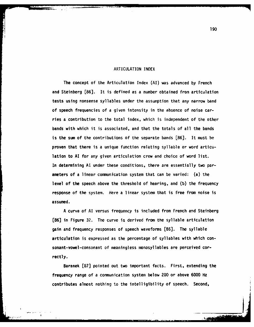
190
ARTICULATION INDEX
The concept of the Articulation Index (AI) was advanced by French
and Steinberg [86]. It is defined as a number obtained from articulation
tests using nonsense syllables under the assumption that any narrow band
of speech frequencies of a given intensity in the absence of noise car-
ries a contribution to the total index, which is independent of the other
bands with which it is associated, and that the totals of all the bands
is the sum of the contributions of the separate bands [86]. It must be
proven that there is a unique function relating syllable or word articu-
lation to Al for any given articulation crew and choice of word list.
In determining Al under these conditions, there are essentially two par-
ameters of a linear communication system that can be varied: (a) the
level of the speech above the threshold of hearing, and (b) the frequency
response of the system. Here a linear system that is free from noise is
assumed.
A curve of Al versus frequency is included from French and Steinberg
[86] in Figure 32. The curve is derived from the syllable articulation
gain and frequency responses of speech waveforms [86]. The syllable
articulation is expressed as the percentage of syllables with which con-
sonant-vowel-consonant of meaningless monosyllables are perceived cor-
rectly.
Baranek [87] pointed out two important facts. First, extending the
frequency range of a communication system below 200 or above 6000 Hz
contributes almost nothing to the intelligibility of speech. Second,
__ _ __ _ __ _ I.'

191
w ~4----
0 Li t-
W N '4-
LL
0
x L)(
wwZ 04-
_ w ~z
0 U.
0r 4J0
C,
0 w
X3WNI NOIIViflDIfl8V 31ISOdWO3

192
each frequency band shown in Table XXV makes a 5 percent contribution to
the Al, provided that the orthotelephonic gain of the system is optimal
(about +10 dB) and that there is no noise present.
TABLE XXV
FREQUENCY BANDS OF EQUAL CONTRIBUTIONTO ARTICULATION INDEX
Mid-Freq Mid-FreqNo. Edges of Band (Mean) No. Edges of Band (Mean)
1 200 - 300 270 11 1600 - 1830 17402 330 - 430 380 12 1830 - 2020 19203 430 - 560 490 13 2020 - 2240 21304 560 - 700 630 14 2240 - 2500 23705 700 - 840 770 15 2500 - 2820 26606 840 - 1000 920 16 2820 - 3200 30007 1000 - 1150 1070 17 3200 - 3650 34008 1150 - 1310 1230 18 3650 - 4250 39509 1310 - 1480 1400 19 4250 - 5050 465010 1480 - 1660 1570 20 5050 - 6100 5600
The orthotelephonic (OT) gain is defined by
OT Gain (Subjective) = 20 log (eo/Po) + 20 log (E2/e0 )
+ 20 log (P1/E2 ) (A.1)
where
P1 = free field pressure necessary to produce the same loudness
in the ear as was to produce by the earphone with voltage
E2 across.
W - -, 6 -.,

193
• o = voltage produced by the microphone across the input re-
sistor of the amplifier by a voice which produces pressure
Po at a distance of one meter in a free field.
E2/eo = voltage amplification of the amplifier.
OT Gain (Objective) = 20 log (eo/po) + 20 log R
+ 20 log (e2/eo ) + 20 log (Pe/e2) (A.2)
where
R = ratio of the pressure produced at the eardrum of a listener
by a source of sound to the pressure which would be produced
by the same source at the listener's head position if he were
removed from the field.
Pe = pressure produced at the eardrum of a listener by the ear-
phone with a voltage e2 across it; others are the same.
The AI obtained per frequency band in Table XXV is successively
added to arrive at the total Al.

APPENDIX D
SONAGRAMS
194

195
ow-

196
lIt 7
197
I L-bI

198
OF
id

I, 199
toI
E .-
g0

200
AM WSW

bib
\ITA
Seqadu L . Ibur, e r..
,.iAdidate Tor the Degree cf
boot.o;" of Philosophy
Thesis: EFFICILET CO[L',C OF -!HE PREDICTION POSIUAL
',i1j or :ield- Elec .ricdl Lwj inecvrin
-I .>hicaL
Per;onae Data: arn in O Ia hj i w 'i (W, aho:. , Au '.st 3. - 94.cthe son of Mr. and ,r7. L. Burge.
Education: Graduated from bouglass Hijh S hooj, Oklaioma City,Oklahoma, in May 1967; received Bachelor of Science degree -nElectrical Engineering from Oklahoma State iniversity in 1972;received Master of Science in Electrical Engineering fromOklahoma State University in 1973; completed requirements forthe Doctor of Philosophy degree at Oklahoma State Universit,in becewiber 1979.
Pro -.-ssional xperience: Eiyineer Trainee, Oklahoma Gas and Uec-tric, summers 1961?-71; student teaching assistant, School UfElectrizal Engineering, Oklahoma State University, 1970-71;graduate teizning assistant, School of Elcctrical Enginetrin 9 ,O(lahoma St.ate Universi.ty, 1911-72; United States Air Force,1?73 t, preent.
Pr-,Ife.sional Organ zal: ons: Member of Institute (if Llectricai andElectronic Engineers, Sigma Xi, Eta Kappa Nu.
.' I-I III---'l-I- --'

-Ell
DATE
FILMED
DTIC