uncovering the plot: detecting surprising coalitions of entities...

Data Mining and Knowledge Discovery manuscript No.(will be inserted by the editor)

Uncovering the Plot: Detecting SurprisingCoalitions of Entities in Multi-Relational Schemas

Hao Wu · Jilles Vreeken · Nikolaj Tatti ·Naren Ramakrishnan

Received: date / Accepted: date

Abstract Many application domains such as intelligence analysis and cyber-security require tools for the unsupervised identification of suspicious entitiesin multi-relational/network data. In particular, there is a need for automatedsemi-automated approaches to ‘uncover the plot’, i.e., to detect non-obviouscoalitions of entities bridging many types of relations. We cast the problemof detecting such suspicious coalitions and their connections as one of miningsurprisingly dense and well-connected chains of biclusters over multi-relationaldata. With this as our goal , we model data by the Maximum Entropy principle,such that in a statistically well-founded way we can gauge the surprisingnessof a discovered bicluster chain with respect to what we already know. Wedesign an algorithm for approximating the most informative multi-relationalpatterns, and provide strategies to incrementally organize discovered patternsinto the background model. We illustrate how our method is adept at discov-ering the hidden plot in multiple synthetic and real-world intelligence anal-ysis datasets. Our approach naturally generalizes traditional attribute-based

H. Wu (�)Department of Electrical and Computer Engineering, Virginia Tech, Arlington, VA, andDiscovery Analytics Center, Virginia Tech, Arlington, VA, USA.E-mail: [email protected]

J. VreekenMax Planck Institute for Informatics, Saarbrucken, Germany, andCluster of Excellence MMCI, Saarland University, Saarbrucken, GermanyE-mail: [email protected]

N. TattiHIIT, Department of Information and Computer Science, Aalto University, Finland, andDepartment of Computer Science, KU Leuven, Leuven, BelgiumE-mail: [email protected]

N. RamakrishnanDepartment of Computer Science, Virginia Tech, Arlington, VA, USA, andDiscovery Analytics Center, Virginia Tech, Arlington, VA, USA.E-mail: [email protected]

2 Hao Wu et al.

maximum entropy models for single relations, and further supports iterative,human-in-the-loop, knowledge discovery.

Keywords Multi-relational data · Maximum entropy modeling · Subjectiveinterestingness · Pattern mining · Biclusters

1 Introduction

Knowledge discovery from multi-relational datasets is a crucial task that arisesin many domains, e.g., intelligence analysis, biological knowledge discovery. Inthe domain of intelligence analysis, questions such as ‘How is a suspect con-nected to the passenger manifest on this flight?’, ‘How do distributed terroristcells interface with each other?,’ are common conundrums faced by analysts.Similarly, ‘how do these two pathways influence each other?’, ‘what is thesignal transduction cascade from an extracellular molecule to an intracellularprotein?’ are typical questions posed by biologists. A pervasive task performedby analysts is thus the laying out of evidence from multiple sources, identifyingcoalitions of entities, incrementally building connections between them, andchaining these connections to create stories that either serve as end hypothesesor as templates of reasoning that can then be prototyped.

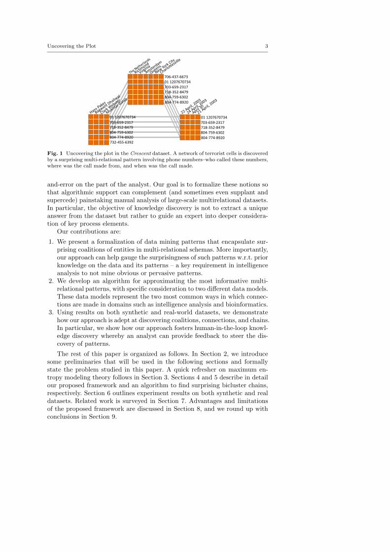
Our work here focuses exclusively on multi-relational datasets, either avail-able in native form or obtained through straightforward ‘relationalization’of unstructured text datasets. We focus on discovering patterns that tie to-gether three inter-related aspects: coalitions (which groups of entities come to-gether?), connections (how do they interface with other groups?), and chains(how do such connections form a chain of evidence?). Fig. 1 illustrates a pat-tern example from the popular Crescent dataset used in intelligence analysis.The hidden plot in this dataset is a distributed and loosely organized networkof terrorist cells that plan to attack multiple cities. As shown, the plot involvesfour coalitions (of phone numbers, dates, people, and places), three relations(who called which number, from where, and when), and the combined chainreveals an odd group of people that turns out to be central to communicationand coordination between the terrorist cells. Note the multiple phone numbersthat were used by the group to coordinate with each other, and by chainingpatterns across the phone number interface we are able to discover the dis-tributed terrorist network. Note also that the chains do not necessarily have tobe perfect to be informative; here there are phone numbers (e.g, 732-455-6392,706-437-6673) not perfectly related to other pieces of evidence, yet the entirechain is surprising enough to alert the analyst to the overall pattern. Similarly,in the domain of bioinformatics, it is easy to imagine coalitions of genes, pro-teins, and other molecules, and where the connections straddle relations suchas transcriptional regulation, signal transduction, and small molecule binding,and the combined chain would indicate a cascade of how extracellular inputsget propagated into downstream cellular responses.

Finding surprising chains as shown in Fig. 1 from multi-relational data hasthus far been considered somewhat of a black art and requires significant trial-

Uncovering the Plot 3

01 1207670734 703-659-2317 718-352-8479 804-759-6302

804-774-8920

01 1207670734 703-659-2317 718-352-8479 804-759-6302

804-774-8920

01 1207670734

703-659-2317 718-352-8479 804-759-6302 804-774-8920 732-455-6392

706-437-6673

Fig. 1 Uncovering the plot in the Crescent dataset. A network of terrorist cells is discoveredby a surprising multi-relational pattern involving phone numbers–who called these numbers,where was the call made from, and when was the call made.

and-error on the part of the analyst. Our goal is to formalize these notions sothat algorithmic support can complement (and sometimes even supplant andsupercede) painstaking manual analysis of large-scale multirelational datasets.In particular, the objective of knowledge discovery is not to extract a uniqueanswer from the dataset but rather to guide an expert into deeper considera-tion of key process elements.

Our contributions are:

1. We present a formalization of data mining patterns that encapsulate sur-prising coalitions of entities in multi-relational schemas. More importantly,our approach can help gauge the surprisingness of such patterns w.r.t. priorknowledge on the data and its patterns – a key requirement in intelligenceanalysis to not mine obvious or pervasive patterns.

2. We develop an algorithm for approximating the most informative multi-relational patterns, with specific consideration to two different data models.These data models represent the two most common ways in which connec-tions are made in domains such as intelligence analysis and bioinformatics.

3. Using results on both synthetic and real-world datasets, we demonstratehow our approach is adept at discovering coalitions, connections, and chains.In particular, we show how our approach fosters human-in-the-loop knowl-edge discovery whereby an analyst can provide feedback to steer the dis-covery of patterns.

The rest of this paper is organized as follows. In Section 2, we introducesome preliminaries that will be used in the following sections and formallystate the problem studied in this paper. A quick refresher on maximum en-tropy modeling theory follows in Section 3. Sections 4 and 5 describe in detailour proposed framework and an algorithm to find surprising bicluster chains,respectively. Section 6 outlines experiment results on both synthetic and realdatasets. Related work is surveyed in Section 7. Advantages and limitationsof the proposed framework are discussed in Section 8, and we round up withconclusions in Section 9.

4 Hao Wu et al.

2 Preliminaries and Problem Statement

Before formalizing our problem statement, we introduce some preliminary con-cepts and notations.

Multi-relational schema We assume that we are given m domains or universeswhich we will denote throughout the paper by Ui. An entity is a member ofUi and an entity set Ei is simply a subset of Ui. We write R = R(Ui, Uj)to be a binary relation between some Ui and Uj . Given a set of domainsU = {U1, U2, . . . , Ul} and a set of relations R = {R1, R2, . . . , Rm}, a multi-relational schema S(U ,R) is a connected bipartite graph whose vertex set isgiven by U ∪R and edge set is the collection of edges each of which connectsa relation Rj in R and a domain Ui in U that the relation Rj involves. In thispaper, without loss of generality, all vertices in R are assumed to have degreeof two, i.e., only binary relationships are considered. As is well known, ternaryand higher-order relations can be converted into sets of binary relationships.(No such degree constraint exists for U ; a domain can participate in manyrelationships.) Figure 2 shows a toy example of a multi-relational schema in-volving four domains (i.e., Phone Numbers, Organizations, People, and Places)and three binary relations (Person–Phone Number, Person–Organization , andOrganization–Place) between these domains.

We now introduce mechanisms to relate entity sets. Redescriptions relateentity sets in the same domain whereas biclusters are ways to relate entity setsacross domains.

Tiles A tile T on binary relationship, a notion introduced by Geerts et al(2004), is essentially a rectangle in a data matrix. Formally, it is defined asa tuple T = (r(T ), c(T )) where r(T ) is a set of row identifier (e.g., row IDs)and c(T ) is a set of column identifier (e.g., column IDs) on the matrix rep-resentation of the binary relationship. In this most general form, it imposesno constraints on values of the matrix elements identified by a tile. So, eachelement in a tile could be either 1 or 0. In Figure 2, T1 is an example of a tile.When all elements within a tile T have the same value (i.e., either all 1s or all0s) we say it is an exact tile. Otherwise we call it a noisy tile.

Biclusters As local patterns of interest over binary data, we consider biclus-ters. A bicluster, denoted by B = (Ei, Ej), on relation R = R(Ui, Uj), consistsof two entity sets Ei ⊆ Ui and Ej ⊆ Uj such that Ei × Ej ⊆ R. As sucha bicluster is a special case of an exact tile, one in which all the elementsare 1. Further, we say a bicluster B = (Ei, Ej) is closed if for every entityei ∈ Ui \ Ei, there is some entity ej ∈ Ej such that (ei, ej) /∈ R and for everyentity ej ∈ Uj \Ej , there is some entity ei ∈ Ei such that (ei, ej) /∈ R. In otherwords, we cannot expand Ei without modifying Ej and vice versa. If a pair ofentities ei ∈ Ui, ej ∈ Uj belongs to a bicluster B, we denote it by (ei, ej) ∈ B.

In Figure 2, B1, B2 and B3 are three biclusters from relation R1, R2 andR3, respectively—T1 is not a bicluster, as not all its elements are 1s.


𝑹𝟏

𝑹𝟐

𝑹𝟑

Ph

on

e N

um

be

rs

Persons

Organ

ization

s

Places

𝑑1 𝑑2

𝑇1

𝐵1

𝐵2

𝐵3

𝑝1

𝑝2

𝐶1

Fig. 2 An example multi-relational schema involving four entity domains (People, Places,Organizations, and Phone Numbers) and three relations (R1, R2, R3). Blue squares indicatepresence in the binary relations, and gray squares indicate absence. Examples of redescrip-tion ((p1, d1) ∼org (p2, d2)), biclusters (B1, B2, B3), tiles (T1), and bicluster chains (C1)are shown.

Redescriptions Assume that we are given two biclusters B = (Ei, Ej) andC = (Fj , Fk), where Ei ⊆ Ui, Ej , Fj ⊆ Uj , and Fk ⊆ Uk. Note that Ej andFj lie in the same domain. Assume that we are given a threshold 0 ≤ ϕ ≤ 1.We say that B and C are approximate redescriptors of each other, whichwe denote by B ∼ϕ,j C if the Jaccard coefficient |Ej ∩ Fj | / |Ej ∪ Fj | ≥ ϕ.The threshold ϕ is a user parameter, consequently we ofter drop ϕ from thenotation and write B ∼j C. The index j indicates the common domain overwhich we should take the Jaccard coefficient. If this domain is clear from thecontext we often drop j from the notation. For example, in Figure 2, we have(p1, d1) ∼ϕ,org (p2, d2) for ϕ ≤ 3/5. If B ∼1,j C, then we must have Ej = Fjin which case we say that B is an exact redescription of C.

This definition is a variant of the definition given by Zaki and Ramakrish-nan (2005), whom define redescriptions for itemsets over their mutual domain,transactions, such that the set Ej consists of transactions containing itemsetEi and the set Fj consists of transactions containing itemset Fk.

Bicluster Chains A bicluster chain C consists of an ordered set of biclusters{B1, B2, . . . , Bk} and an ordered bag of domain indices {j1, j2, . . . , jk−1} suchthat for each pair of adjacent biclusters we have Bi ∼ji Bi+1. Note that thisimplicitly require that two adjacent biclusters share a common domain.

In Figure 2, C1 is an example of a bicluster chain comprising three biclus-ters, viz., B1, B2 and B3. If a bicluster BRi is a part of the bicluster chain C,we will represent this by BRi

∈ C in this paper.

6 Hao Wu et al.

Surprisingness In data mining the main goal is to extract novel knowledge.That is, we aim to find results that are highly informative with regard to whatwe already know—we are not so much interested in what we already do know,or what we can trivially induce from such knowledge.

To this end, we suppose a probability distribution p that represents theuser’s current beliefs about the data. When mining the data (e.g., for a bi-cluster or chain), we can use p to determine the likelihood of a result underour current beliefs: if it is high, this indicates that we most likely alreadyknow about it, and thus, reporting it would provide little new information. Incontrast, if the likelihood of a result is very low, the result is very surprising,which means it conveys a lot of new information. In Section 3, we will discusshow to infer such a probability distribution for binary data. First, we formallydefine the problem we consider in this paper.

Problem Statement Given a multi-relational dataset, a bicluster chain acrossmultiple relations describes a progression of entity coalitions. We are particu-larly interested in chains that are surprising w.r.t. what we already know, asthese could help to uncover the plots hidden in the multi-relational dataset.

More formally, given a multi-relational dataset schema S(U ,R), where U ={U1, U2, . . . , Ul} and R = {R1, R2, . . . , Rm}, we are interested to find K non-redundant bicluster chains that are most surprising with regard to each otherand w.r.t. the background knowledge:

Given: Multi-relational Dataset Schema S(U ,R)Find: K Bicluster Chains C = {C1, C2, . . . , CK}

such that C is non-redundant and surprisingwith respect to the background knowledge ofS(U ,R).

Next, we first discuss how to probabilistically model binary data using theMaximum Entropy principle. In Section 4 we will use this model to developscores for bicluster chains, while in Section 5 we will discuss strategies forefficiently mining surprising bicluster chains from data.

3 MaxEnt Models for Binary Data

Our problem statement is based on a notion of multi-relational schema. Fortechnical reasons we will base our score, however, on binary datasets. Morespecifically, we assume that our schema was generated from a transactionalbinary data matrix D. This data matrix can be viewed as a binary matrix ofsize N -by-M . We will introduce two ways of obtaining a schema from D inSection 4.1. In both of these approaches the columns of D correspond to theentities of the schema. Hence, we will refer to the columns of D as entities.

In this section, we will define the Maximum Entropy (MaxEnt) model forbinary data using tiles as background knowledge—recall that a tile is a moregeneral notion than a bicluster. We will first introduce notation that will be


useful to understand the model derivation. Then, we will recall MaxEnt theoryfor modelling binary data given tiles as background information, and finally,identify how we can fit the model to the data by maximizing the likelihood.

3.1 Notation for Tiles

Given a binary dataset D of size N -by-M and a tile T , the frequency of T inD, fr(T ;D), is defined as

fr(T ;D) =1

|σ(T )|∑

(i,j)∈σ(T )

D(i, j) . (1)

Here, D(i, j) represents the entry (i, j) in D, and σ(T ) = {(i, j) | i ∈ r(T ), j ∈c(T )} denotes the cells covered by tile T in data D. Recall that a tile T iscalled ‘exact’ if the corresponding entries D(i, j) ∀(i, j) ∈ σ(T ) are all 1 (resp.0), or in other words, fr(T ;D) = 0 or fr(T ;D) = 1. Otherwise, it is called a‘noisy’ tile.

Let D be the space of all the possible binary datasets of size N -by-M , andp be the probability distribution defined over the dataset space D. Then, thefrequency of the tile T with respect to p is

fr(T ; p) = E [fr(T ;D)] =∑D∈D

p(D)fr(T ;D) , (2)

the expected frequency of tile T under the dataset probability distribution.Combining these definitions, we have the following lemma.

Lemma 1 Given a dataset distribution p and a tile T , the frequency of tile Tis

fr(T ; p) =1

|σ(T )|∑

(i,j)∈σ(T )

p ((i, j) = 1) ,

where p((i, j) = 1) represents the probability of a dataset having 1 at entry(i, j) under the dataset distribution p.

Lemma 1 is trivially proved by substituting fr(T ;D) in Equation (2) withEquation (1) and switching the summations.

3.2 Global MaxEnt Model from Tiles

Here, we will construct a global statistical model based on tiles. Suppose weare given a set of tiles T , and each tile T ∈ T is associated with a frequencyγT—which typically can be trivially obtained from the data. This tile set Tprovides information about the data at hand, and we would like to infer adistribution p over the space of possible datasets D that conforms with theinformation given in T . That is, we want to be able to determine how probableis a dataset D ∈ D given the tile set T .

8 Hao Wu et al.

To derive a good statistical model, we take a principled approach and em-ploy the Maximum Entropy principle (Jaynes, 1957) from information theory.Loosely speaking, the MaxEnt principle identifies the best distribution givenbackground knowledge as the unique distribution that represents the providedbackground information but is maximally random otherwise. MaxEnt mod-elling has recently become popular in data mining as a tool for identifying sub-jective interestingness of results with regard to background knowledge (Wangand Parthasarathy, 2006; De Bie, 2011; Tatti and Vreeken, 2012).

To formally define a MaxEnt distribution, we first need to specify thespace of the probability distribution candidates. Here, these are all the possibledataset distributions that are consistent with the information contained inthe tile set T . Hence, the dataset distribution space is defined as: P = {p |fr(T ; p) = γT ,∀T ∈ T }. Among all these possible distributions, we choose thedistribution p∗T that maximizes the entropy,

p∗T = arg maxp∈P

H(p) .

Here, H(p) represents the entropy of the dataset probability distribution p,which is defined as

H(p) = −∑D∈D

p(D) log p(D) .

Next, to infer the MaxEnt distribution p∗T , we rely on a classical theoremabout how MaxEnt distributions can be factorized. In particular, Theorem3.1 in (Csiszar, 1975) states that for a given set of testable statistics T (back-ground knowledge, here a tile set), a distribution p∗T is the Maximum Entropydistribution if and only if it can be written as

p∗T (D) ∝

{exp

( ∑T∈T

λT · |σ(T )| · fr(T ;D))D 6∈ Z

0 D ∈ Z ,

where λT is a certain weight for fr(T ;D) and Z is a collection of datasets suchthat p(D) = 0, for all p ∈ P.

De Bie (2011) formalized the MaxEnt model for a binary matrix D givenrow and column margins—also known as a Rasch (1960) model. Here, weconsider the more general scenario of binary data and tiles, for which weadditionally know (Theorem 2 in Tatti and Vreeken, 2012) that given a tileset T , with T (i, j) = {T ∈ T | (i, j) ∈ σ(T )}, we can write the distributionp∗T as

p∗T =∏

(i,j)∈D

p∗T ((i, j) = D(i, j)) ,

where

p∗T ((i, j) = 1) =exp

(∑T∈T (i,j) λT

)exp

(∑T∈T (i,j) λT

)+ 1

or 0, 1 .


This result allows us to factorize the MaxEnt distribution P ∗T of binary datasetgiven background information in the form of a set of tiles T into a productof Bernoulli random variables, each of which represents a single entry in thedataset D. We should emphasize here that this model is different MaxEntmodel than when we assume independence between rows in the dataset D (see,e.g., Tatti, 2006; Wang and Parthasarathy, 2006; Mampaey et al, 2012). Here,for example, in the special case where the given tiles are all exact (γT = 0 or1), the resulting MaxEnt distribution will have a very simple form:

p∗T ((i, j) = 1) =

{γT if ∃T ∈ T such that (i, j) ∈ σ(T )12 otherwise.

3.3 Inferring the MaxEnt Distribution

To discover the parameters of the Bernoulli random variable mentioned above,we follow a standard approach and apply the well known Iterative Scaling(IS) algorithm (Darroch and Ratcliff, 1972) to infer the tile based MaxEntdistribution on binary dataset. Basically, for each tile T ∈ T , the algorithmupdates the probability distribution p such that the expected frequency of 1sunder distribution p for that will match the given frequency γT . Clearly, duringthis update we may change the expected frequency for other tiles, and henceseveral iterations are needed until the probability distribution p converges. Forthe proof of algorithm convergence, please refer to Theorem 3.2 in (Csiszar,1975). In practice, it typically takes on the order of seconds for the algorithmto converge.

4 Scoring Bicluster Chains

We now turn our attention to using the above formalisms to help score ourpatterns, viz., bicluster chains. But before we do so, we need to pay attentionto the schemas over which these chains are inferred, as this influences howchains can be represented as tiles, in order to be incorporated as knowledge inour maximum entropy model.

4.1 Data Model Specification

In this section, we describe two approaches to construct multi-relational schemasS(U ,R) from binary transaction data D. Whenever an element D(r, ei) hasvalue 1, this denotes that entity ei appears in row r of D. As an example, whenconsidering text data, an entity would correspond to a word or concept, and arow to a document in which this word occurs. (Thus, note that when consid-ering text data we currently model occurrences of entities at the granularityof documents. Admittedly, this is a coarse modeling in contrast to modelingoccurrences at the level of sentences, but it suffices for our purposes.)

10 Hao Wu et al.

… … … … … …

… … … …

… … … … … …

… … … …

… …

…

… D

ocs

𝑈1 Doc-Entity model

… …

… … … … … …

… … … …

… …

… …

…

…

… …

…

…

… …

Binary data matrix D

Do

cs

𝑈1 𝑈𝑙 … 𝑈𝑖 … 𝑈𝑙

… …

…

…

… …

𝑒ℎ 𝑒𝑘

𝑒 ℎ

𝑒 𝑘

𝑈𝑖

Entity-Entity model

𝑒𝛼 𝑒𝜖 𝑒𝜏 𝑒𝛼 𝑒𝜖 𝑒𝜏

Fig. 3 Illustration of the two data models. The entities marked with red, orange, green, andblack squares in matrix D appear together in some documents, thus, induce the, resp., red,orange, green, and black squares in the Entity–Entity model on the right, respectively. Thedata marked with large brown rectangular in matrix D involves only one type of entities(U1), which results the Doc–Entity model on the left. See Figure 4 for a toy example.

Entity-Entity model

Doc-Entity model Binary data matrix D

Fig. 4 Toy example of how to construct our two data models from a binary matrix D.

Entity–Entity Model. In the Entity–Entity data model, each binary rela-tion in R stores the entity co-occurrences in data matrix D between two entitydomains. More specific, for each R = R(Ui, Uj) in R, (e, f) ∈ R for e ∈ Ui,f ∈ Uj , and e and f appear at least once together in a row in D. The right-hand side of Figure 3 illustrates this data model for the example transactionalbinary data matrix D depicted in the middle.

Example 1 We illustrate how to construct this model using the toy exam-ple depicted in Figure 4. We show the Entity–Entity model (right) for thetoy data matrix D (middle). The binary data matrix D consists of 4 docu-ments (rows) over 7 entities (columns) which belong to two entity domains:Organizations and Persons. We observe entities Robinson and Grant of entitydomain Persons appear together with entities Nasdaq and CNN of domainOrganizations in document Doc2 in D (marked with red squares). For the cor-responding Entity–Entity model this hence induces the four relation instances(Robinson,Nasdaq), (Robinson,CNN ), (Grant ,Nasdaq) and (Grant ,CNN )(also marked with red square) in the Persons-Organizations relation on theright-hand side of the figure. Analogue, the person entity Jack and organiza-tion entity FBI (marked with yellow squares) appear together in documentDoc4, which induces the relation instance (Jack ,FBI ) (marked with yellowsquare) in the bottom-right corner of Persons-Organizations relation.

Doc–Entity Model. In the Doc–Entity data model, we treat the rows inD as a special entity domain, UD, in the multi-relational schema S(U ,R).


More in particular, rows in D are considered the common interconnectingentity domain relating the rest of the other entity domains, and leads to a‘unidirectional’ schema—unlike, say the schema shown in Fig. 2. In this datamodel, each binary relation in R contains the entity occurrence information ofeach entity domain in binary data matrix D. For every R = R(UD, Ui) in R,(r, e) ∈ R for r ∈ UD, e ∈ Ui, and transaction r contains entity e in the datamatrix D, D(r, ek) = 1. Figure 3 illustrates the concepts of the Doc–Entity(left) model for the given data matrix D (middle).

Example 2 Let us also illustrate the Doc–Entity model using the toy data de-picted in Figure 4. We show the Doc–Entity model (left) for the given data ma-trix D (middle). As D consists of two entity types (Persons and Organizations)the Doc–Entity model consists of two relations, i.e., Document-Organizationand Document-Person—which contain the exact same entity occurrence in-formation as left (marked with brown square) and right (marked with greensquare) hand sides of data matrix D.

Here, every pair of biclusters naturally shares a common domain, the doc-uments UD. Hence, any pair of biclusters B = (Ei, ED) and C = (Fj , FD)here redescribe each other iff B ∼ϕ,D C. Further, in practice we only considerchaining biclusters that share a single domain, and hence for this model havethat the bag of domain indices associated with the chain consists of only D’s.

4.2 When is What Model Applicable?

The choice of whether to use the Entity–Entity versus the Doc–Entity modelcarries many ramifications. At first glance, it might appear that a biclusterin the Entity–Entity model must be equivalent to a bicluster chain (of twobiclusters) in the Doc–Entity model. To see why this is not so, consider whatit means to be a bicluster in each of these models. In the Entity–Entity model,a bicluster (Ei, Ej) captures two sets of entities that co-occur, but the co-occurrence could be derived from many different documents. In contrast, inthe Doc–Entity model, a bicluster chain relating entity sets Ei and Ej mustdo so using the same or a significantly overlapping set of documents. It ishence instructive to view the Entity–Entity model as a ‘multiple source ofevidence’ model, whereas the Doc–Entity model is a ‘common domain’ model.The former better integrates disparate sources of evidence, each of which maynot be significant in itself. The latter provides stronger evidence for inferenceand is consequentially stricter in evidence integration. As we will show in ourresults, both models have uses in intelligence analysis.

4.3 Background Model Definition

Next, to discover non-trivial and interesting bicluster chains, we need to in-corporate some basic information about the multi-relational schema S(U ,R)

12 Hao Wu et al.

into the model. As such basic background knowledge over D we use the col-umn marginals, and the row marginals per entity domain. To this end, follow-ing Tatti and Vreeken (2012) we construct a tile set Tcol consisting of a tileper column, a tile set Trow consisting of a tile per row per entity domain, anda tile set Tdom consisting of a tile per entity domain but spanning all rows.Formally, we have

Tcol = {(UD, e) | e ∈ U,U ∈ U \ {UD}} ,

Trow = {(r, U) | r ∈ UD, U ∈ U \ {UD}} , and

Tdom = {(UD, U) | U ∈ U \ {UD}} .

We refer to the combination of these three tile sets as the background tile setTback = Trow ∪ Tcol ∪ Tdom . Given the background tiles Tback , the backgroundMaxEnt model Pback can be inferred using Iterative Scaling (see Sect. 3.3).

Example 3 Using again the toy data of Figure 4, a tile in Tcol would be({Doc1 ,Doc2 ,Doc3 , Doc4}, {Nasdaq}), a tile in Trow would be ({Doc1},{Nasdaq ,CNN ,FBI }), and a tile in Tdom would be ({Doc1 ,Doc2 ,Doc3 ,Doc4},{Nasdaq ,CNN ,FBI }).

4.4 Assessing the Quality of a Bicluster Chain

To assess the quality of a given bicluster chain C with regard to our backgroundknowledge, we need to first convert it into tiles such that we can infer thecorresponding MaxEnt model. Below we specify how we do this conversion foreach of our two data models.

Entity–Entity Model: For each bicluster B ∈ C in a chain C, with B =(Ei, Ej), we construct a tile set TB , consisting of |Ei| |Ej | tiles, as follows

TB = {(rows(X;D), X) | X = {ei, ej} with (ei, ej) ∈ B} , (3)

where rows(X;D) is the set of rows that contain X in D. The tile set thatcorresponds to a bicluster chain C is then TC =

⋃B∈C TB .

Example 4 Considering the example Entity–Entity bicluster B = ({Robinson,Grant}, {Nasdaq ,CNN }) in Figure 4, the entity Robinson from Person do-main and entity Nasdaq from Organization domain appear together in Doc2in the data matrix D. Thus, rows({Robinson,Nasdaq};D) = {Doc2}, andthe related tile would be ({Doc2}, {Robinson,Nasdaq}). Following the similarlogic, the tile set TB corresponding to the example bicluster B would be

TB = {({Doc2}, {Robinson,Nasdaq}),({Doc2}, {Robinson,CNN }),({Doc2}, {Grant ,Nasdaq}),({Doc2}, {Grant ,CNN })} .


Doc–Entity Model: For the Doc–Entity model, we only have to constructa single tile TC to represent a bicluster chain C, with

TC =

( ⋃(ED,Ei)∈C

ED ,⋃

(ED,Ei)∈C

Ei

), (4)

where each ED is a set of documents, ED ⊆ UD, each entity set Ei ⊆ Ui, andB = (ED, Ei) is a bicluster in chain C. Note that unions are well defined inEq. 4 since ED are subsets of UD, the domain corresponding to the transac-tions, while the domains of Ei together consistute the items of the dataset.Trivially, the tile set corresponding to the bicluster chain C is TC = {TC}.

Example 5 Considering the example bicluster chain C = {({Doc1 ,Doc2},{Nasdaq ,CNN }), ({Doc2 ,Doc3}, {Robinson,Grant})} in the Doc–Entity modelin Figure 4 as an example, the tile representing this bicluster chain for theDoc–Entity model is

TC = ({Doc1 ,Doc2 ,Doc3}, {Nasdaq ,CNN ,Robinson,Grant}) .

4.5 Measuring Relative Quality

To determine the relative quality of a bicluster chain Ci ∈ C in a set of bi-cluster chains C—for example, to rank results—we propose to calculate itsrelative importance: how much novel information does Ci provide in contrastto our background knowledge and the rest of the chain? We will do this byinferring two probability distributions using MaxEnt, and then calculating thedivergence between these distributions.

More formally, we first infer a MaxEnt model Pfull based on all available in-formation. That is, Pfull is based on Tback∪TC , where TC = {TC1 , TC2 , . . . , TCK

}and K = |C|. Next, we infer a second MaxEnt model PCi based on all informa-tion except Ci; that is, we infer PCi

based on Tback and TC\Ci= {TC1

, TC2, . . . ,

TCi−1, TCi+1

, . . . , TCK}. Finally, we measure the divergence between these two

models. To this end, we choose the Kullback-Leibler (KL) divergence (Coverand Thomas, 2006), that is KL(Pfull || PCi ), as it is well understood, and fitsour setup both in goal as well as with regard to ease of computation. In theory,however, other divergence measures could be considered.

5 Searching For Good Chains

In this section, we will describe the strategy to find interesting bicluster chainsfrom multi-relational dataset schema. In theory, to discover a set of interestingbicluster chains C we could exhaustively explore the search space and evaluateeach and every bicluster chain. Clearly, however, the number of possible biclus-

ter chains is prohibitively large; their number is in the order of O(∏|R|i=1 |Bi|)

where Bi is the set of biclusters, which are eligible to form bicluster chains,

14 Hao Wu et al.

Algorithm 1: Greedy Inference of Bicluster Chainsinput : background MaxEnt model Pback ;

Ball = {Bi} where Bi is a set of biclusters from Ri in R;K, the desired number of bicluster chains.

output: set of bicluster chains C.1 C ← ∅;2 while (|C| < K) do3 Rstart ← mostBiclusterRelation(R);4 B∗start ← findStartBicluster(Rstart);5 C ← B∗start ;6 B ← eligibleBiclusters(Ball , C);7 while |B| 6= 0 do8 B∗ ← arg max

B∈Bsglobal (B);

9 C ← addToChain(C, B∗);10 B ← eligibleBiclusters(Ball , C);

11 end12 Pback ← UpdateMaxEntModel(Pback , C);13 C ← C ∪ {C};14 end15 C ← SortChains(C);

from relation Ri in R. This number explodes if either the number of relations|R|, or the number of candidate biclusters |Bi| is non-trivial. Moreover, thesearch space does not exhibit structure (e.g. monotonicity) that we can exploitfor efficient search. Hence, we resort to heuristics.

We employ a simple iterative greedy search, that, as we will see, works wellin practice. First we define how to greedily choose bicluster candidates makinguse of our MaxEnt model. Given a bicluster B, we generate a correspondingset of tiles TB . This conversion is different between our two data models.

Entity–Entity Data Model. When considering the Entity–Entity model,we generate the tile set TB according to the definition in Equation (3).

Doc–Entity Data Model. When considering the Doc–Entity model, the bi-cluster B already represents the tile and hence we use TB = {B}.

Next, we measure how much information TB gives with regard to the back-ground model Pback . We define the following score,

sglobal(B) = KL(PB ||Pback ) , (5)

where PB is the MaxEnt model inferred on both tile sets Tback and TB . Asthis score measures the amount of information B adds with regard to the fulldata, we refer to this score as the global score. The larger sglobal(B) is, themore new information B contains—and, we say, the more likely B is a goodcandidate to form an interesting bicluster chain.

Next, we explain our search strategy for mining interesting bicluster chains.Algorithm 1 illustrates the algorithm. Starting from the relation in R that has


the most biclusters (Line 3), say Rstart , we choose the bicluster B∗start fromRstart as starting bicluster for a bicluster chain such that the score defined inEquation (5) is maximized (Line 4), that is,

B∗start = arg maxB⊆Rstart

sglobal(B) .

Given a starting bicluster B∗start that serves as the first bicluster in our chain C,we proceed as follows. From all relations in R not yet covered by a B ∈ C, weselect the set of biclusters B ⊂ Ball that we can add to C. That is, we considerevery B(Ei, Ej) ∈ Ball over relation R(Ui, Uj) for which a) the current chainC does not already include a bicluster over relation R(Ui, Uj), and b) whichare redescriptions of either the first bicluster Bfirst ∈ C, or the last biclusterBlast ∈ C in chain C. We extend C with the most informative bicluster B∗ ∈ B,with

B∗ = arg maxB∈B

sglobal(B) .

We then iterate; we re-calculate the set of eligible biclusters B (Line 10), andcontinue to find the next bicluster B∗ to add to C. The search stops when thechain cannot be extended further, i.e., when B is empty.

During this search process, we need to score every candidate bicluster B ∈B. When using sglobal this implies we have to infer a MaxEnt model for eachand every candidate, which is computationally expensive. Moreover, sglobal

evaluates a candidate globally, whereas typically most information is local :only few entries in MaxEnt distribution will be affected by adding B into themodel. Making use of this observation, to reduce the computation cost of thechain search procedure, we define the score slocal(B) that measures the localsurprisingness of a tile set as

slocal(B) = −∑T∈TB

∑(i,j)∈σ(T )

log p∗((i, j) = D(i, j)) , (6)

where p∗((i, j) = D(i, j)) is the MaxEnt probability defined by the backgroundmodel. Compared with the previous score defined in Equation (5), this localscore does not require re-infer MaxEnt model for each bicluster B ∈ B, andwill hence greatly reduce the time needed by the search.

Once a chain C is completed, we update the background MaxEnt modelPback to not re-discover C or chains with close resemblance again (Line 12).1 Werepeat the search process until we have completed finding the top-K biclusterchains, where K is specified by the user. Finally, the set of bicluster chainsC mined from the multi-relational dataset is reordered based on the qualitymeasure defined in Section 4.5 (Line 15).

1 Note that, to save computation, we do not update the MaxEnt model after adding eachB∗. However, in line with the local score, we know that adding a bicluster typically onlychanges the distribution locally, and as we never re-visit the same relation R in a singlechain C the information by Bi is unlikely to influence much the informativeness of Bi+1.

16 Hao Wu et al.

Table 1 Dataset Statistics

Number ofDocuments

Number ofEntities

Doc–Entity Entity–Entity

Dataset %1s min %1s max %1s

Synthetic 1k 1000 1000 0.01 — 0.05 0.01 0.05Synthetic 2k 2000 2000 0.01 — 0.05 0.01 0.05Synthetic 3k 3000 3000 0.01 — 0.05 0.01 0.05Synthetic 5k 5000 5000 0.01 — 0.05 0.01 0.05Synthetic 10k 10000 10000 0.01 — 0.05 0.01 0.05

Atlantic Storm 111 716 0.0179 0.0261 0.0608Crescent 41 284 0.0425 0.0357 0.136Manpad 47 143 0.0299 0.0385 0.0714

Computation Complexity To mine a single chain, at worst case we evaluateevery eligible bicluster in every Ri ∈ R against our MaxEnt model—i.e., every

bicluster in B =⋃|R|i=1 Bi. That is, we have a worst case complexity of O(v ·|B|),

where v is the time needed to evaluate the surprisingness of a single biclusterand depends on whether global or local score is used. When using the globalscore, Eq. (5), v is characterized by the convergence time of the MaxEnt modelPB when evaluating bicluster B. When using the local score, Eq. (6), v statis-tically relies on the average size of the biclusters under consideration (whichimplicitly depends on the density of data matrix D). To mine K biclusterchains, the number of bicluster evaluations is O(K · |B|). While constructingthe chain, determining whether a bicluster is an admissible redescription takesO(1) time. All combined, the computation complexity of the greedy searchprocess is O(v ·K · |B|). Using the global score we have to re-infer the Max-Ent model for every eligible bicluster B, while for the local score only aftercompleting a chain.

6 Experiments

We describe experimental results over both synthetic and real datasets. Forreal datasets, we focus primarily on datasets from the domain of intelligenceanalysis, although as stated in the introduction, our framework is broadlyapplicable to many relational data mining contexts. The focuses of our exper-imental investigations are to answer the following questions:

i. Can the proposed framework discover planted bicluster chains from multi-relational datasets? (Section 6.1)

ii. How does the framework’s runtime scale with increasing size and densityof the dataset? (Section 6.2)

iii. Does the approach help reveal plots hidden in real data? (Section 6.3)

iv. How does the proposed framework perform against a baseline method?(Section 6.4)

v. Can our approach foster human-in-the-loop knowledge discovery? (Sec-tion 6.5)


0.01 0.02 0.03 0.04 0.050

0.2

0.4

0.6

0.8

1

relation density β

reca

ll

α=1α=2α=3

0.01 0.02 0.03 0.04 0.050

0.2

0.4

0.6

0.8

1

relation density β

prec

isio

n

α=1α=2α=3

Fig. 5 Recall (left) and Precision (right) scores for the Entity–Entity model on Syntheticdata of N = 1000 by M = 1000, of l = 5 different types of 200 entities each.

All the experiments described were conducted on a Xeon 2.0 Ghz machinewith 528 GB memory. Performance results were obtained by averaging over10 independent runs. We give the basic statistics of the datasets we use inTable 1. We make the implementation and real datasets publically availablefor research purposes.2

6.1 Synthetic Data

To evaluate against known ground truth and with control over the data char-acteristics, we generate synthetic data. The synthetic datasets are param-eterized as follows. The binary data matrix D consists of N rows and Mcolumns, or entities, which we divide into l different domains. For the Doc–Entity data model, we then have U = {UD, U1, U2, . . . , Ul} and R = {Ri =R(UD, Ui) | i = 1, 2, . . . , l}. For the Entity–Entity data model, we set thedataset schema S(U ,R) to contain l − 1 inter-entity relationships such thatRi = R(Ui, Ui+1), i = 1, 2, . . . , l − 1. That is, two adjacent inter-relationshipsRi and Ri+1 share a common entity domain Ui+1. These relationships can beextracted from D based on entity co-occurrences.

To verify whether our proposed framework can indeed discover true bi-cluster chains, we generate the synthetic datasets as follows. The binary datamatrix D is first constructed with N = 1000 and M = 1000, with l = 5 entitydomains of τ = 200 entities each. As ground truth, α bicluster chains acrossall the binary relations Ri ∈ R are constructed. The rows and columns of eachbicluster in the chain are randomly sampled from the domains that Ri ∈ Rinvolves. A Jaccard coefficient of ϕ = 0.75 is maintained between the adjacentbiclusters in the chain. In this experiment, we varied α from 1 to 3. Then,these bicluster chains are planted into the binary data matrix D. Finally, foreach entry in D that is not covered by the planted true bicluster chains, wesample its values from a Bernoulli distribution with parameter β′ dependent

2 http://dac.cs.vt.edu/projects

18 Hao Wu et al.

1 2 3 4 5 6 7 8 9 101.28

1.3

1.32

1.34

1.36

1.38x 105

number of discovered chains

(neg

ativ

e)lo

g−lik

elih

ood

global scorelocal scoretrue chains

Fig. 6 [Lower is better] Negative log-likelihood scores of the data under the MaxEnt model,for Synthetic data of 1000-by-1000, of 5 different types of entities with 200 entities pertype, and 5 planted bicluster chains. The relation density is β = 0.03. The decrease of the(negative) log-likelihood indicates the MaxEnt model is more certain about the data.

on Ri—which allows us to control the density β of the binary relations. In thisset of experiments, the binary relation density β was varied from 0.01 to 0.05.

To discover the planted chains from the synthetic data, we first considerthe global score as defined in Equation (5). As input to our algorithm we firstmine candidate biclusters by applying the lcm algorithm (Uno et al, 2005)to each binary relation—note that any bicluster mining algorithm for binarydata is applicable. When constructing the chains, we use a Jaccard coefficientthreshold of ϕ = 0.75 to determine whether two biclusters are approximateredescriptions, and as we are aiming to recover all platned bicluster chains weset K = α. We find that for each of the scenarios described above our approachcorrectly recovers all planted bicluster chains.

Figures 5 shows the recall and precision with regard to entities—the pro-portion of entities of the planted chains discovered by our approach, resp. theproportion of entities in the discovered chains also in the planted chains—forEntity–Entity modeling. We observe that precision decreases slightly with in-creased density, which stems from cliques being less detectable in more densedata. Due to the random data generation process, and the greedy search, wemay observe effects that recall locally increases for higher density. Overall thetrend we observe corresponds with intuition: for higher density data it is moredifficult to find correct chains, as dense areas are more likely to be createdat random. For the Doc–Entity model, the results are perfect, in that bothprecision and recall are always 1 over all parameter settings, as our frameworkfinds the exact planted true bicluster chains in each of these scenarios. (Asthese figures are visually not very interesting, we omit them.)

To further investigate how well our approach works in general, and toevaluate both the global and local scores, we run our method on syntheticdata as above, planting 5 bicluster chains. We show in Figure 6 the (negative)log-likelihood scores of this data under the MaxEnt models per discovered


0.01 0.02 0.03 0.04 0.050

1

2

3

4

5

6

relation density (β)

time

(sec

ond)

N=1000,τ=200N=2000,τ=400N=3000,τ=600

0.01 0.02 0.03 0.04 0.050

50

100

150

200

250


time(

seco

nd)

N=1000,τ=200N=2000,τ=400N=3000,τ=600

Fig. 7 Time to infer the MaxEnt model (left) resp. time to search for chains (right) onSynthetic data over 5 entity domains, 1 planted chain, and of differing density β.

chain. We calculate the likelihood as follows

−∑

(i,j)∈D

log p∗T ((i, j) = D(i, j)) . (7)

We find that the chains discovered using both the global and local scoresvery closely match the true chains, and hence do the likelihood scores. More-over, for both scores the likelihood converges at the true number of chains; thismeans both that we can determine whether all significant bicluster chains havebeen discovered, as well as that standard model selection techniques, such asBIC (Schwarz, 1978) or MDL (Rissanen, 1978) are applicable for automaticallyidentifying the correct number of chains in the data.

As a negative result, we report that for Synthetic data with a relationdensity β > 0.1, we discover only partial chains; likely the (relatively small)planted biclusters do not sufficiently stand out from the dense background.We did not encounter this problem for real data, as they are typically (very)sparse.

6.2 Runtime and Scalability

To evaluate the scalability of our method with regard to different data charac-teristics, we applied our approach on synthetic datasets of 1000 up to 10 000rows and columns, and varying the relation densities β from 0.01 to 0.05. Wekeep the number of entity domains and planted bicluster chains fixed at 5 and1, respectively. We first evaluate only using our global score.

We first investigate the time needed to infer the MaxEnt model, and thetime to search for chains (Figure 7) for datasets of resp. 1000, 2000, and 3000rows and columns. The figure shows that these aspects are stable with regardto relation density. Figure 8 (left) shows that, as expected, computation mostlydepend on the size of the data, and that less time is needed to rank the finalchains for more dense. In Figure 8 (right) we summarize the total run timeof our approach. Most importantly, in Figure 9 we show that the local score

20 Hao Wu et al.

0.01 0.02 0.03 0.04 0.050

2

4

6

8

10


time

(sec

ond)

N=1000,τ=200N=2000,τ=400N=3000,τ=600

0.01 0.02 0.03 0.04 0.050

50

100

150

200

250

300


time

(sec

ond)

N=1000,τ=200N=2000,τ=300N=3000,τ=600

Fig. 8 Time to rank discovered chains (left) resp. total run-time (right) on Synthetic dataof 5 entity domains, 1 planted chain and of differing density β.

1k by 1k 3k by 3k 5k by 5k 10k by 10k10

0

101

102

103

size of matrix D

time

(sec

ond)

α = 1α = 2α = 3

local score

global score

Fig. 9 Scalability comparison between the global and local scores on Synthetic data ofdensity β = 0.03, over 5 entity domains, for resp. α = 1, 2, and 3 planted chains.

is more than one order of magnitude faster than the global score; while itgenerally attains results of equally high quality.

Overall run times are reasonable and within the order of minutes. Moreover,the framework allows for trivial parallelization, e.g., over calculating the scoresfor all candidates (Line 8 in Algorithm 1).

6.3 Real Data

Next we investigate the performance on real data. To be able to evaluate thediscovered chains qualitatively we consider three intelligence analysis datasets:AltanticStorm (Hughes, 2005), Manpad, and Crescent (Hughes, 2005). Thetask for these datasets is to discover the plots of any imminent threat, armsdealing, or possible terrorist attacks. Note the highly unstructured nature ofknowledge discovery in these datasets. We pre-process these datasets in threesteps: (i) co-reference resolution, i.e., resolving entities refering to the sameobject (e.g., a proper noun upon introduction of the entity and a pronoun at a


…

…

• Abdellah Atmani, who works for Holland Orange Shipping Lines, helps in smuggling the biological agents to the Caribbean from Morocco.

• Jose Escalante and Arze received training together before in Havana, Cuba. Carlos Morales has been suspected of associations with Cuban intelligence. All these three involve transferring biological agents from Bahamas to USA.

• Fahd al Badawi, Boris Bugarov, Adnan Hijazi, Jose Escalante and Saeed Hasham coordinate with each other to recruit Al Qaeda field agents to transport biological agents to USA via Holland Orange Shipping Lines.

Fig. 10 Top-ranked bicluster chains and related plots for the AtlanticStorm dataset. Thebottom chain was found using the Entity–Entity model, the top two using the Doc–Entitymodel. Entities in bold (red) are part of the true solution.

later reference), (ii) entity extraction and classification into categories, usingthe standard NLP tool AlchemyAPI,3 and (iii) transforming the data into ourDoc–Entity and Entity–Entity data models. To select candidate biclusters inthe chain construction process, we here use a Jaccard coefficient of ϕ = 0.5,which ensures a wide variety of chains can be discovered from the noisy realdatasets.

Figure 10 shows the top few bicluster chains found by our proposed frame-work on the AtlanticStorm dataset. The two small bicluster chains at the top,from the Doc–Entity data model, reveal connections between three persons:

3 http://www.alchemyapi.com/

22 Hao Wu et al.

• Mark Davis, who lives at 2462 Myrtle Ave. in Queens, NYC, and works at Empire State Vending Service (ESVS), services the vending machines at New York Stock Exchange (NYSE).

• Bagwant Dhaliwal, who lives at 2462 Myrtle Ave. in Queens, NYC and is employed by ESVS, fought with Taliban in 1990-1992.

• Hani al Hallak manages a carpet store in North Bergen, NJ, and has a phone with number 732-455-6392.

• Several recent calls were made to Hani al Hallak’s phone from 718-352-8479, which is associated with the address 2462 Myrtle Ave. in Queens, NYC. In most recent call from 718-352-8479, the caller said he would pick up the carpet on 25 April, 2003.

• A fire happened at Hani al Hallak’s carpet shop, where C-4 is discovered in the basement.

• Mark Davis is also known as Hamid Alwan, a Suadi national, who received explosives training in Sudan and Afghanistan.

Fig. 11 Top-ranked bicluster chain and related plots for the Crescent dataset. Entities inbold (red) are part of the true solution.

Carlos Morales, Arze and Jose Escalante, and the connections between theperson Abdellah Atmani and the company Holland Orange Shipping Lines.These two bicluster chains lead us to the central plots of the AtlanticStormdataset: namely, that Jose Escalante, Arze, Carlos Morales and Abdellah At-mani are involved in transferring biological agents to United States. The largebicluster chain at the bottom of Fig. 10, discovered using the Entity–Entitydata model, reveals the connections among the persons Fahd al Badawi, BorisBugarov, Jose Escalante, Adnan Hijazi and Saeed Hasham and the organiza-tions of Holland Orange Shipping Lines and Al Qaeda, which identifies theplot of these five persons to recruit Al Qaeda members to transport biologicalagents to the USA via Holland Orange Shipping Lines.

The bicluster chain in Figure 11 is the top one discovered from the Crescentdataset under the Entity–Entity data model. This bicluster chain shows theconnections among three persons (Mark Davis, Hani al Hallak and BagwantDhaliwal), two Companies (Empire State Vending Services (ESVS) and NewYork Stock Exchange (NYSE)), and an address (Myrtle Ave. in Queens, NewYork City). It turns out one plot related to a terrorist action in Crescentdataset is Mark Davis, who has received explosive training before, and Bagwant


Table 2 Recall scores on three real datasets for three different chain discovery methods.For these datasets the plots do not form coherent chains, and hence we report and discussthe precision, and the subtle issues regarding this, in Section 6.4.

Our Approach

Dataset BigCluster InfPair InfCluster

Atlantic Storm 0.32 0.16 0.32Crescent 0 0.29 0.86Manpad 0.14 0.21 0.36

Dhaliwal, who fought with Taliban in 1990-1992, will pick up C-4 bombs fromHani al Hallak on April 25, 2003, and plan to install the C-4 onto vendingmachines at NYSE. Thus, the bicluster chain shown here helps to uncover thishidden plot in the Crescent dataset.

6.4 Baseline Comparisons

Though there exist studies on the general topic of ‘finding plots’, e.g.,Shahafand Guestrin (2010, 2012); Hossain et al (2012b); Kumar et al (2006); Hossainet al (2012a), we consider a quite distinct problem setting for which to thebest of our knowledge no existing approach is applicable. (See Section 7 for acomplete discussion of related work.) To demonstrate the effectiveness of ourapproach, we hence compare to two baselines.

The first baseline method, BigCluster, follows Algorithm 1 to find biclus-ter chains yet iteratively chooses to extend the chain with the largest biclusterinstead of determining subjective interestingness using MaxEnt. As a secondbaseline we consider a simplified version of our method, we consider InfPair,which performs like InfCluster but iteratively finds the most informativeentity pair to add to the chain, as opposed to the most informative bicluster.

We apply the three methods to each of the three real datasets, and considerthe recall with regard to entities and the precision with regard to chains—the proportion of the discovered chains related to the dataset solution—forthe top-3 discovered chains. We use this definition here, as unlike for thesynthetic data in these real datasets the ‘plots’ do not (necessarily) from onecoherent chain. (See Section 8 for a more in-depth discussion of the difficultiesof evaluating our problem setting.) We first discuss the recall scores, which wegive in Table 2. Overall, our main approach InfCluster consistently identifiesthe best chains. With its simplified variant InfPair in second place this showsthat a good bicluster chain is not simply the combination of large biclusters—and that surprisingness is an important aspect to obtain interesting results.As we only consider the top-3 chains discovered in a single iteration, precisionis a less interesting metric here—the scores possible per dataset are resp. 0,13 , 2

3 , and 1. Averaged over the three datasets, we find that BigCluster hasa precision of 0.33, InfPair a precision of 0.78, and InfCluster a precision

24 Hao Wu et al.

• Homer W., who is a member of Aryan Brotherhood of Colorado, sells the weapons to John H., who is a member of Al-Queda, in Colorado.

• Arnold C. (Abu H.)., who was a suspect of the 9/11 attack and spent time in Afghanistan, rents a U-Hual truck and drives it from Boulder, Colorado to Los Angeles. He probably transports the weapons.

• Ralph T., who is a member of Aryan Militia, bought weapons and sells them to George W. (Muhammad J.) who is a member of Al-Queda.

• Ralph T. meets Kamel J. in Atlanta, Georgia, and Kamel J. drives a truck from Atlanta to St. Paul, Minnesota. He probably transports weapons.

𝐶2 : 𝐶1:

𝐶3: . . .

𝐶1′:

𝐶1

User Feedback

𝐶2

𝐶3

Fig. 12 Iterative mining on the Manpad Dataset. Entities in bold (red) are part of thetrue solution. The top two bicluster chains were selected by the analyst from the top-rankeddiscovered chains, and then incorporated as background knowledge, leading to discovery ofa new bicluster chain at the bottom revealing a sub-plot in the dataset.

of 0.56. The difference between InfPair and InfCluster is explained byInfPair considering much smaller biclusters than InfCluster. Consideringboth precision and recall InfCluster performs best with a wide margin.

6.5 Case Study for Iterative Human-in-the-Loop Data Mining

Having verified the quality of our framework and InfCluster in particular,we now investigate its performance for iterative human-in-the-loop discoveryof interesting bicluster chains in a small case study. To this end we considerthe Manpad dataset and ask an in-house domain expert to analyze the datawith our tool. We give the key results for the first iterations in Figure 12.

We mined the top-3 of bicluster chains and presented these to the expert,whom selected those she finds interesting; here, the two top-ranked biclusterchains, depicted at the top of the figure are the two top-ranked chains dis-covered in the first iteration, were selected. After identifying that these twobicluster chains reveal the plots of two separate arms dealings in Boulder,Colorado and Atlanta, Georgia, and that the weapons are transported to LosAngeles in California and St. Paul in Minnesota for potential terrorist at-tacks, the analysts add these two chains back into the model as part of the


1 2 3 40.2

0.3

0.4

0.5

0.6

0.7

0.8

Iterations

Rec

all

ManpadAtlanticStormCrescent

1 2 3 40

0.2

0.4

0.6

0.8

1

Iterations

Pre

cisi

on

ManpadAtlanticStormCrescent

Fig. 13 Recall (left) and precision (right) of true plot entities vs. number of iterations forresp. the Manpad, AtlanticStorm, and Crescent datasets. Please note that in the right panelthe lines of Manpad and Crescent datasets overlap.

background knowledge, and further investigate the dataset to discover otherrelated plots. With the updated background information, our framework re-computes the bicluster chains, and discovers as the top-ranked bicluster chainthe one shown at the bottom of Figure 12, revealing a plot involving anotherarm dealing between the persons John H. and Homer W. in Colorado.

As the iterative discovery process continues, the intelligence analyst findsmore and more entities involved in the plots of the intelligence dataset. Wegive the recall with regard to important entities and precision with regardto chains over the first four iterations in Figure 13 for each the Manpad, At-lanticStorm and Crescent datasets. From the figure we see that the recall ofimportant entities steadily increases with further iterations, indicating thatmore and more of the entire plots are discovered. Note that while desirable, itis not realistic to expect 100% recall—unless the plot is trivial, stands out verystrongly from the background knowledge, and no other significant structuresare present in the dataset. Investigating the relatively modest recall scoresfor Crescent we find these are due to key structure of the data is reported inthe first few iterations that is unrelated to the plot yet unexplained by thebackground knowledge.

7 Related Work

In this section we survey related work. In particular, we discuss work relatedwith regard to mining biclusters, surprising patterns, iterative data mining,mining multi-relational datasets, and finding plots in data.

7.1 Mining Biclusters

Mining biclusters is an extensively studied area of data mining, and many al-gorithms for mining biclusters from all sorts of data types have been proposed.Tibshirani et al (1999) proposed a backward pruning method to find biclusters

26 Hao Wu et al.

with constant values. While, Califano et al (2000) aimed to find biclusters withconstant values on rows or columns, which they defined as σ-valid ks-patterns.Segal et al (2001) and Sheng et al (2003) investigated mining biclusters withina Bayesian framework and using probabilistic relational models. Cheng andChurch (2000) proposed an algorithm to find the δ-biclusters—which is de-fined by the mean squared residue between rows and columns of the cluster.Regarding the biclustering algorithms on binary data, Zaki and Hsiao (2005)proposed an efficient algorithm called Charm-L for mining frequent closeditemsets and their lattice structure. Uno et al (2005) developed the lcm algo-rithm that combines the data structures of array, bitmap and prefix trees toefficiently discover frequent as well as closed itemsets. A comprehensive surveyof biclustering algorithms was given by Madeira and Oliveira (2004).

Bicluster mining, however, is not the primary aim in this paper; instead it isonly a component in our proposed framework. Moreover, the above mentionedstudies do not assess whether the mined clusters are subjectively interesting.

7.2 Mining Surprising Patterns

There is, however, significant literature on mining representative/succinct/sur-prising patterns (e.g., Kiernan and Terzi, 2008) as well as on explicit summa-rization (e.g., Davis et al, 2009). Wang and Parthasarathy (2006) summarizeda collection of frequent patterns by means of a row-based MaxEnt model,heuristically mining and adding the most significant itemsets in a level-wisefashion. Tatti (2006) showed that querying such a model is PP-hard. Mampaeyet al (2012) gave a convex heuristic, allowing more efficient search for the mostinformative set of patterns. De Bie (2011) formalized how to model a binarymatrix by MaxEnt using row and column margins as background knowledge,which allows efficient calculation of probabilities per cell in the matrix. Thesepapers all focus on mining surprising patterns from a single relation. They donot explore the multi-relational scenario, and can hence not find connectionsamong surprising patterns from different relations—the problem we focus on.

7.3 Iterative Data Mining

Iterative data mining as we study was first proposed by Hanhijarvi et al (2009).The general idea is to iteratively mine the result that is most significant givenour accumulated knowledge about the data. To assess significance, they buildupon the swap-randomization approach of Gionis et al (2007) and evaluateempirical p-values. Tatti and Vreeken (2012) discussed comparing the infor-mativeness of results by different methods on the same data. They gave aproof-of-concept for single binary relations, for which results naturally trans-late into tiles, and gave a MaxEnt model in which tiles can be incorporated asbackground knowledge. In this work we build upon this framework, translatingbicluster chains (over multiple relations) into tiles to measure surprisingnesswith regard to background knowledge using a Maximum Entropy model.


7.4 Multi-relational Mining

Mining relational data is a rich research area (Dzeroski and Lavrac , editors)with a plethora of approaches ranging from relational association rules (De-haspe and Toironen, 2000) to inductive logic programming (ILP) (Lavrac andFlach, 2001). The idea of composing redescriptions (Zaki and Ramakrishnan,2005) and biclusters to form patterns in multi-relational data was first pro-posed by Jin et al (2008). Cerf et al (2009) introduced DataPeeler algorithmto tackle the challenge of directly discovering closed patterns from n-ary re-lations in multi-relational data. Later, Cerf et al (2013) refined DataPeelerfor finding both closed and noise-tolerant patterns. These frameworks do notprovide any criterion for measuring subjective interestingness of the multi-relational patterns.

Ojala et al (2010) studied randomization techniques for multi-relationaldatabases with the goal to evaluate the statistical significance of databasequeries. Spyropoulou and De Bie (2011) and Spyropoulou et al (2014) proposedto transform a multi-relational database into a K-partite graph, and to mineMaximal Complete Connected Subset (MCCS) patterns that are surprisingwith regard to a MaxEnt model based on the margins of this data. Spyropoulouet al (2013) extended this approach to finding interesting local patterns inmulti-relational data with n-ary relationships.

Bicluster chains and MCCS patterns both identify redescriptions betweenrelations, but whereas MCCS patterns by definition only identify exact pair-wise redescriptions (completely connected subsets), bicluster chains also allowfor approximate redescriptions (incompletely connected subsets). All except forthe most simple bicluster chains our methods discovered in the experiments ofSection 6 include inexact redescriptions, and could hence not be found underthe MCCS paradigm. Besides that we consider two different data models,another key difference is that we iteratively update our MaxEnt model toinclude all patterns we mined so far. Mampaey et al (2012) and Kontonasioset al (2013) show that ranking results using a static MaxEnt model leads toredundancy in the top-ranked results, and that iterative updating provides aprincipled approach for avoiding this type of redundancy.

7.5 ‘Finding Plots’

Finally, we give an overview of work on discovering ‘plots’ in data. Note thatthe key difference between finding plots, and finding biclusters or surprisingpatterns is the notion of chaining patterns into a chain, or plot.

Commercial software such as Palantir provide significant graphic and visu-alization capabilities to explore networks of connections but do not otherwiseautomate the process of uncovering plots from document collections. Shahafand Guestrin (2012) studied the problem of summarizing a large collection ofnews articles by finding a chain that represents the main events; given either astart or end-point article, their goal is to find a chain of intermediate articles

28 Hao Wu et al.

that is maximally coherent. In contrast, in our setup we know neither the startnor end points. Further, in intelligence analysis, it is well known that plots areoften loosely organized with no common all-connecting thread, so coherencecannot be used as a driving criterion. Most importantly, we consider data ma-trices where a row (or, document) may be so sparse or small (e.g., 1-paragraphsnippets) that it is difficult to calculate statistically meaningful scores. Story-telling algorithms (e.g., Hossain et al, 2012b; Kumar et al, 2006; Hossain et al,2012a) are another related thread of research; they provide algorithmic waysto rank connections between entities but do not focus on entity coalitions andhow such coalitions are maintained through multiple sources of evidence.

8 Discussion

From the results on synthetic as well as real data, we find that our framework isable to correctly identify highly interesting bicluster chains from unstructureddata. Performance is best for the Doc–Entity model, which is partly due tothe MaxEnt modelling process adhering closer to this setup, as well as that forthe Entity–Entity model it is inherently more complex to find good bi-clusters.Still, the results on real data for both models provide much insight and usefulinformation about the plots hidden in the data.

To score the surprisingness of biclusters our current approach requires thatthe input data can be transformed into a flat binary table—which we thenmodel by Maximum Entropy. As here we consider text data as our input forus this transformation is straightforward and without loss for the Doc–Entitymodel. While such transformation into binary data is always possible—we can,e.g., model the adjacency matrix of (un)directed graphs—the more closelythe modelling follows the input data, the better. It will be interesting to seewhether it is possible to extend our approach to include different MaxEntmodels for different relations. With regard to the Entity–Entity model, weidentify the need for MaxEnt theory to model integer-valued, or count data asthen we can determine the surprisingness of how often entities co-occur. Therecent results by Kontonasios et al (2011, 2013) on modelling continuous valueddata by MaxEnt seems a natural starting point as the model can incorporatetiles as background knowledge.

While it has very nice theoretic properties, and performs well in practice,calculating our global objective score is computationally expensive. To this endwe proposed local approximations, which we found to closely approximate theperformance of the global score in practice. To further gain efficiency, one couldevaluate candidates in parallel, as well as parallelize inferring the MaxEntmodels. However, we should also emphasize here that the focus of this paper isexploratory analysis of multi-relational data, and discovering interesting multi-relational patterns in particular. In this study our main concern was quality;follow-up studies can consider scaling our framework up for application tovery large data. With regard to higher quality, we are currently investigatingtheory and methods for directly discovering surprising biclusters; that is, to


take the current MaxEnt model into account when searching for candidateclusters to add to the chain. Currently, our theory and methods are onlydirectly applicable to discrete binary data, other data types will have to befirst transformed to our data models. Here, we used standard NLP tools totransform text into binary relations, without optimizing these towards optimaldetectability of the most interesting bicluster chains. It will make for engagingfuture work to investigate how to optimally transform text for analysis usingour framework.

8.1 Doc–Entity vs. Entity–Entity

From the results on the intelligence datasets, we can see that our proposedframework is capable of identifying important hidden plots with associatedevidence. We observed that if the dataset contains several key entities that arecentral to the plot (such as coordinating several activities), the Doc–Entitydata model will help us to identify these. The Entity–Entity data model onthe other hand reveals more the interactions between different types of entities.Even if some key roles and actions appear only a few times in the data, thisapproach has the potential to uncover the evidence leading to such key play-ers in the dataset. This is mostly because the Entity–Entity model implicitlyputs more on the surprisingness of entities and their coalitions/connectionsin the dataset, whereas traditional methods, such as measuring support andfrequency, cannot really capture. As future work, it may be worthwhile to in-vestigate whether a combination of the two data models is possible, and if thiswould provide better results.

8.2 Exploration vs. Exploitation

As real datasets are typically rather complex, they may contain many possible‘plots’—hence, it is not guaranteed that all the solution entities will naturallyform a single chain without involving other entities. Moreover, for other enti-ties found by our approach that are not in the solution, they cannot be simplydetermined as important or useless. It really depends on whether these enti-ties are connected to the solution entities. For example, in the bicluster chainshown in Figure 11, the entities New York Stock Exhange (NYSE) and EmpireState Vending Services (ESVS) appear together with the important personsMark Davis, Hani al Hallak and Bagwant Dhaliwal. This gives the analystssome hints that something suspecious may happen in NYSE or ESVS. It turnsout to be that Mark Davis who is an employee at ESVS and serves vendingmachines at NYSE plans to get bombs from Hani al Hallak and BagwantDhaliwal, and installs them in the vending machine of NYSE. This demon-strates that if such relevant entities (NYSE, ESVS, etc.) appear together withthe important entities in the dataset, they may provide additional informationto the intelligence analysts. But, if appearing individually, they may not draw

30 Hao Wu et al.

our attention at all. Thus, we could not simply treat such entities as importantor irrelevant entities, which makes the entity precision not be an appropriateevaluation criterion in our scenario. We identify this as a natural aspect ofdata exploration: our method simply identifies what is surprising in the datawith regard to the provided background knowledge, and as long as a discov-ered chain identifies significant structure—whether about the plot of interest,or explaining another aspect of the data—we regard it as a good result.

9 Conclusion and Future Work

Our approach to discover multi-relational patterns is a significant step in for-malizing a previously unarticulated knowledge discovery problem. We haveprimarily showcased results in intelligence analysis, however, the theory andmethods we presented is applicable for analysis of unstructured or discretemulti-relational data in general—such as for biological knowledge discoveryfrom text. The key requirement to apply our methods is that the data can betransformed into one of our two data models. That is, data for which ‘entities’and/or ‘documents’ can be identified. We have presented new data model-ing primitives, algorithms for extracting patterns, and experimental results onscalability as well as effectiveness of inference.

Some of the directions for future work include (i) obviating the need tomine all biclusters prior to composition, (ii) improving accuracy of estimationwhen data density becomes larger, (iii) integrating the two data models intro-duced here, (iv) incorporating weights on relationships, to account for differingveracities and trustworthiness of evidence. Ultimately, the key to a good toolfor data analysts is to foster human-in-the-loop knowledge discovery which isone of the key advantages of the methods proposed here.

Acknowledgements Jilles Vreeken is supported by the Cluster of Excellence “MultimodalComputing and Interaction” within the Excellence Initiative of the German Federal Gov-ernment.

Bibliography

Califano A, Stolovitzky G, Tu Y (2000) Analysis of gene expression microar-rays for phenotype classification. In: Proc. Int. Conf. Intell. Syst. Mol. Biol,pp 75–85

Cerf L, Besson J, Robardet C, Boulicaut JF (2009) Closed patterns meet n-aryrelations. ACM Transactions on Knowledge Discovery from Data 3(1):3:1–3:36

Cerf L, Besson J, Nguyen KNT, Boulicaut JF (2013) Closed and noise-tolerant patterns in n-ary relations. Data Mining and Knowledge Discovery26(3):574–619


Cheng Y, Church GM (2000) Biclustering of expression data. In: Proceedingsof the Eighth International Conference on Intelligent Systems for MolecularBiology, AAAI Press, pp 93–103

Cover T, Thomas J (2006) Elements of Information Theory. WileyCsiszar I (1975) I-Divergence geometry of probability distributions and mini-

mization problems. The Annals of Probability 3(1):pp. 146–158Darroch JN, Ratcliff D (1972) Generalized iterative scaling for log-linear mod-

els. The Annals of Mathematical Statistics 43(5):pp. 1470–1480Davis WLI, Schwarz P, Terzi E (2009) Finding representative association rules

from large rule collections. In: Proceedings of the 9th SIAM InternationalConference on Data Mining (SDM), Sparks, NV, SIAM, pp 521–532

De Bie T (2011) Maximum entropy models and subjective interestingness:an application to tiles in binary databases. Data Mining and KnowledgeDiscovery 23(3):407–446

Dehaspe L, Toironen H (2000) Discovery of relational association rules. In:Dezeroski S (ed) Relational Data Mining, Springer-Verlag New York, Inc.,pp 189–208

Dzeroski S, Lavrac (editors) N (2001) Relational Data Mining. Springer, BerlinGeerts F, Goethals B, Mielikainen T (2004) Tiling databases. In: Proceedings

of Discovery Science, Springer, pp 278–289Gionis A, Mannila H, Mielikainen T, Tsaparas P (2007) Assessing data mining

results via swap randomization. ACM Transactions on Knowledge Discoveryfrom Data 1(3):167–176

Hanhijarvi S, Ojala M, Vuokko N, Puolamaki K, Tatti N, Mannila H (2009)Tell me something I don’t know: randomization strategies for iterativedata mining. In: Proceedings of the 15th ACM International Conferenceon Knowledge Discovery and Data Mining (SIGKDD), Paris, France, ACM,pp 379–388

Hossain M, Gresock J, Edmonds Y, Helm R, Potts M, Ramakrishnan N(2012a) Connecting the dots between PubMed abstracts. PLoS ONE 7(1)

Hossain MS, Butler P, Boedihardjo AP, Ramakrishnan N (2012b) Storytellingin entity networks to support intelligence analysts. In: Proceedings of the18th ACM International Conference on Knowledge Discovery and Data Min-ing (SIGKDD), Beijing, China, ACM, pp 1375–1383

Hughes FJ (2005) Discovery, Proof, Choice: The Art and Science of the Processof Intelligence Analysis, Case Study 6, “All Fall Down”, unpublished report

Jaynes ET (1957) Information theory and statistical mechanics. Physical Re-view Series II 106(4):620–630

Jin Y, Murali TM, Ramakrishnan N (2008) Compositional mining of mul-tirelational biological datasets. ACM Transactions on Knowledge Discoveryfrom Data 2(1):2:1–2:35

Kiernan J, Terzi E (2008) Constructing comprehensive summaries of largeevent sequences. In: Proceedings of the 14th ACM International Conferenceon Knowledge Discovery and Data Mining (SIGKDD), Las Vegas, NV, pp417–425

32 Hao Wu et al.

Kontonasios KN, Vreeken J, De Bie T (2011) Maximum entropy modelling forassessing results on real-valued data. In: Proceedings of the 11th IEEE In-ternational Conference on Data Mining (ICDM), Vancouver, Canada, IEEE,pp 350–359

Kontonasios KN, Vreeken J, De Bie T (2013) Maximum entropy models foriteratively identifying subjectively interesting structure in real-valued data.In: Proceedings of the European Conference on Machine Learning and Prin-ciples and Practice of Knowledge Discovery in Databases (ECML PKDD),Prague, Czech Republic, Springer, pp 256–271

Kumar D, Ramakrishnan N, Helm RF, Potts M (2006) Algorithms for sto-rytelling. In: Proceedings of the 12th ACM International Conference onKnowledge Discovery and Data Mining (SIGKDD), Philadelphia, PA, pp604–610

Lavrac N, Flach P (2001) An Extended Transformation Approach to Induc-tive Logic Programming. ACM Transactions on Computational Logic Vol.2(4):pages 458–494

Madeira SC, Oliveira AL (2004) Biclustering algorithms for biological dataanalysis: A survey. IEEE/ACM Trans Comput Biol Bioinformatics 1(1):24–45

Mampaey M, Vreeken J, Tatti N (2012) Summarizing data succinctly withthe most informative itemsets. ACM Transactions on Knowledge Discoveryfrom Data 6:1–44

Ojala M, Garriga GC, Gionis A, Mannila H (2010) Evaluating query resultsignificance in databases via randomizations. In: Proceedings of the 10thSIAM International Conference on Data Mining (SDM), Columbus, OH, pp906–917

Rasch G (1960) Probabilistic Models for Some Intelligence and AttainnmentTests. Danmarks paedagogiske Institut

Rissanen J (1978) Modeling by shortest data description. Automatica14(1):465–471

Schwarz G (1978) Estimating the dimension of a model. The Annals of Statis-tics 6(2):461–464

Segal E, Taskar B, Gasch A, Friedman N, Koller D (2001) Rich probabilisticmodels for gene expression. Bioinformatics 17(suppl 1):S243–S252

Shahaf D, Guestrin C (2010) Connecting the dots between news articles. In:Proceedings of the 16th ACM International Conference on Knowledge Dis-covery and Data Mining (SIGKDD), Washington, DC, ACM, pp 623–632

Shahaf D, Guestrin C (2012) Connecting two (or less) dots: Discovering struc-ture in news articles. ACM Transactions on Knowledge Discovery from Data5(4):24:1–24:31

Sheng Q, Moreau Y, De Moor B (2003) Biclustering microarray data by gibbssampling. Bioinformatics 19(suppl 2):ii196–ii205

Spyropoulou E, De Bie T (2011) Interesting multi-relational patterns. In:Proceedings of the 11th IEEE International Conference on Data Mining(ICDM), Vancouver, Canada, pp 675–684


Spyropoulou E, De Bie T, Boley M (2013) Mining interesting patterns in multi-relational data with n-ary relationships. In: Discovery Science, Lecture Notesin Computer Science, vol 8140, Springer Berlin Heidelberg, pp 217–232

Spyropoulou E, De Bie T, Boley M (2014) Interesting pattern mining in multi-relational data. Data Min Knowl Discov 28(3):808–849

Tatti N (2006) Computational complexity of queries based on itemsets. Infor-mation Processing Letters 98(5):183–187, DOI http://dx.doi.org/10.1016/j.ipl.2006.02.003

Tatti N, Vreeken J (2012) Comparing apples and oranges - measuring differ-ences between exploratory data mining results. Data Mining and KnowledgeDiscovery 25(2):173–207

Tibshirani R, Hastie T, Eisen M, Ross D, Botstein D, Brown P (1999) Clus-tering methods for the analysis of dna microarray data. Tech. rep., StanfordUniversity

Uno T, Kiyomi M, Arimura H (2005) Lcm ver.3: Collaboration of array, bitmapand prefix tree for frequent itemset mining. In: Proceedings of the 1st Inter-national Workshop on Open Source Data Mining: Frequent Pattern MiningImplementations, ACM, New York, NY, USA, OSDM ’05, pp 77–86

Wang C, Parthasarathy S (2006) Summarizing itemset patterns using proba-bilistic models. In: Proceedings of the 12th ACM International Conferenceon Knowledge Discovery and Data Mining (SIGKDD), Philadelphia, PA, pp730–735

Zaki M, Hsiao CJ (2005) Efficient algorithms for mining closed itemsets andtheir lattice structure. IEEE Transactions on Knowledge and Data Engi-neering 17(4):462–478

Zaki MJ, Ramakrishnan N (2005) Reasoning about sets using redescriptionmining. In: Proceedings of the 11th ACM International Conference onKnowledge Discovery and Data Mining (SIGKDD), Chicago, IL, ACM, pp364–373