Under the Covers:Tuning and Physical Storage

Zachary G. IvesUniversity of Pennsylvania

CIS 550 – Database & Information Systems

November 3, 2003

Some slide content may be courtesy of Susan Davidson, Dan Suciu, & Raghu Ramakrishnan

2

Resuming Last Week’s Discussionof Data Integration…

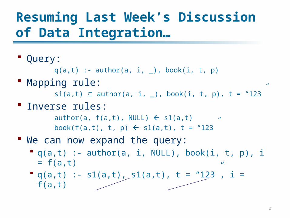
Query: q(a,t) :- author(a, i, _), book(i, t, p)

Mapping rule:s1(a,t) author(a, i, _), book(i, t, p), t = “123”

Inverse rules:author(a, f(a,t), NULL) s1(a,t)

book(f(a,t), t, p) s1(a,t), t = “123”

We can now expand the query: q(a,t) :- author(a, i, NULL), book(i, t, p), i = f(a,t) q(a,t) :- s1(a,t), s1(a,t), t = “123”, i = f(a,t)

3

Query Answering Using Inverse Rules

Invert all rules Take the query and the possible rule

expansions and execute them in a Datalog interpreter: This creates a union of all possible “view

unfoldings”: every possible way of combining and cross-correlating info from different sources all combinations of expansions of book and of author

in our example Then it throws away all unsatisfiable rewritings

(some expansions will be logically inconsistent) The answer is the result of executing the query

4

Faster Algorithms

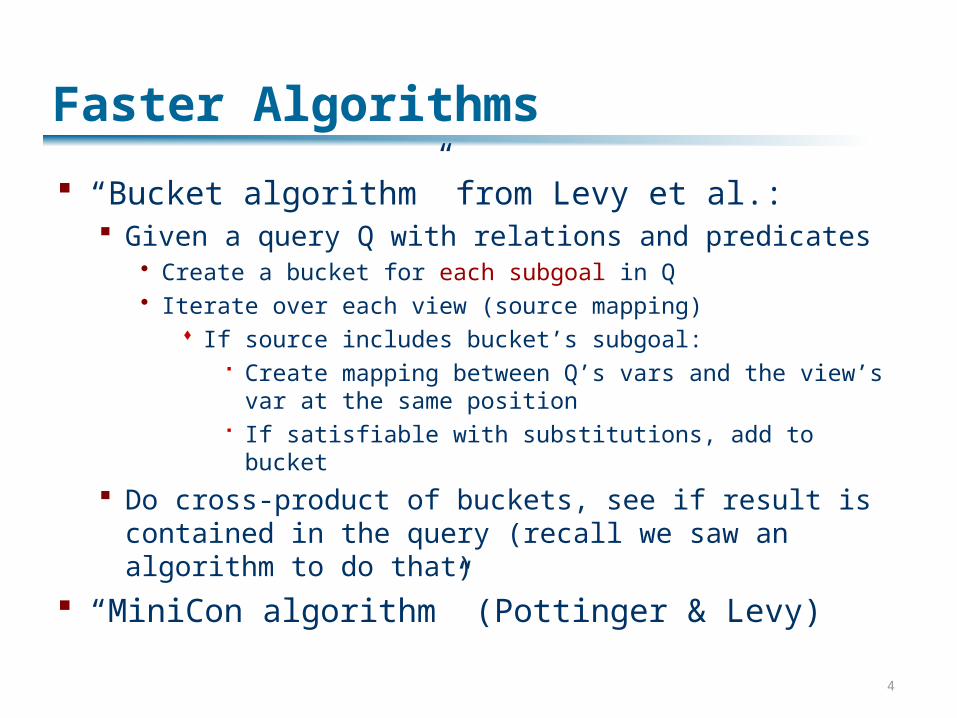
“Bucket algorithm” from Levy et al.: Given a query Q with relations and predicates

Create a bucket for each subgoal in Q Iterate over each view (source mapping)

If source includes bucket’s subgoal: Create mapping between Q’s vars and the

view’s var at the same position If satisfiable with substitutions, add to bucket

Do cross-product of buckets, see if result is contained in the query (recall we saw an algorithm to do that)

“MiniCon algorithm” (Pottinger & Levy)

5

Source Capabilities

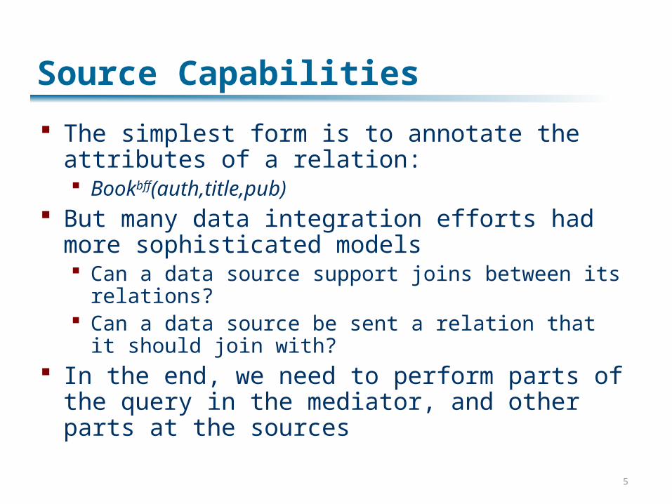
The simplest form is to annotate the attributes of a relation: Bookbff(auth,title,pub)

But many data integration efforts had more sophisticated models Can a data source support joins between its

relations? Can a data source be sent a relation that it should

join with? In the end, we need to perform parts of the

query in the mediator, and other parts at the sources

6

Local-as-View and the Info Manifold

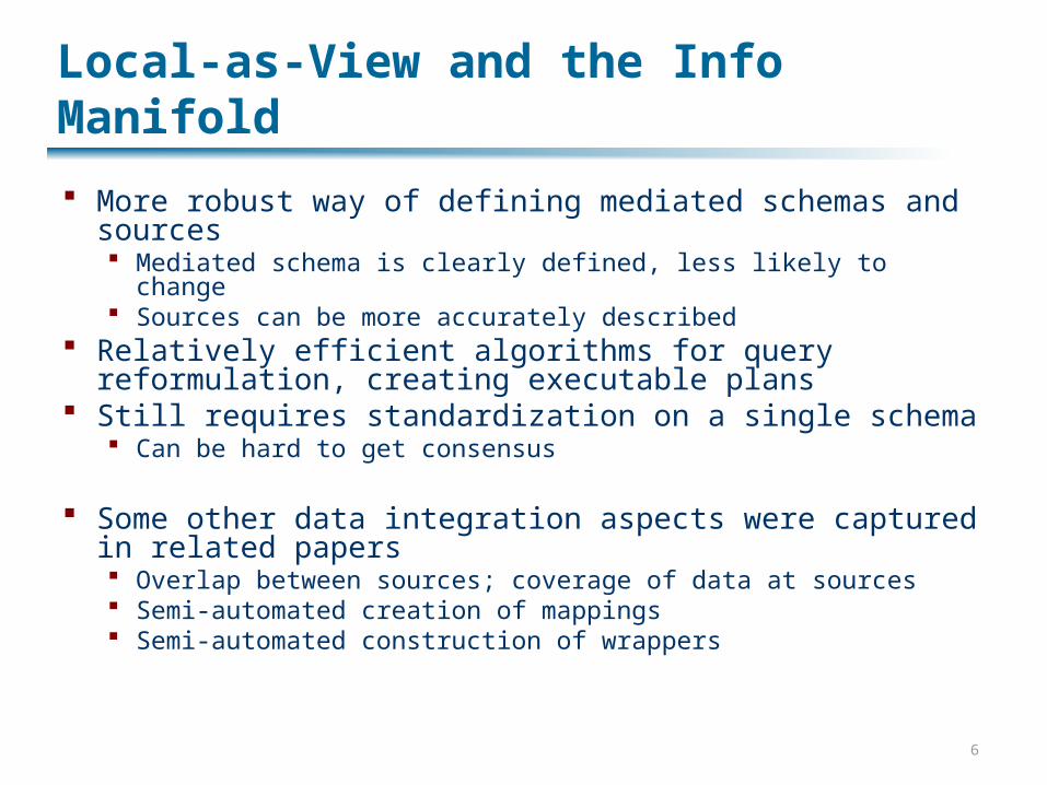
More robust way of defining mediated schemas and sources Mediated schema is clearly defined, less likely to change Sources can be more accurately described

Relatively efficient algorithms for query reformulation, creating executable plans

Still requires standardization on a single schema Can be hard to get consensus

Some other data integration aspects were captured in related papers Overlap between sources; coverage of data at sources Semi-automated creation of mappings Semi-automated construction of wrappers

7

Data Integration, Concluded

A very important problem today – perhaps the central problem faced by most IT departments, scientific collaborations

A basic set of techniques cover many kinds of mappings Concordance tables View-based mappings: local- and global-as-

view Still a field with much ongoing research

Especially at Penn, U. Washington, U. Illinois, UC San Diego

Under the Covers:Tuning and Physical Storage

Zachary G. IvesUniversity of Pennsylvania

CIS 550 – Database & Information Systems

November 3, 2003

Some slide content may be courtesy of Susan Davidson, Dan Suciu, & Raghu Ramakrishnan

9

Performance: What Governs It?

Speed of the machine – of course! But also many software-controlled factors that we

must understand: Caching and buffer management How the data is stored – physical layout, partitioning Auxiliary structures – indices Locking and concurrency control (we’ll talk about this

later) Different algorithms for operations – query execution Different orderings for execution – query optimization Reuse of materialized views, merging of query

subexpressions – answering queries using views; multi-query optimization

10

General Emphasis of Today’s Lecture

Goal: cover basic principles that are applied throughout database system design

Use the appropriate strategy in the appropriate placeEvery (reasonable) algorithm is good somewhere

… And a corollary: database people reinvent a lot of things and add minor tweaks…

11

What’s the “Base” in “Database”?

Could just be a file with random access What are the advantages and

disadvantages?

DBs generally require “raw” disk access Need to know when a page is actually

written to disk, vs. queued by the OS Predictable performance, less fragmentation May want to exploit striping or contiguous

regions Typically divided into “extents” and pages

12

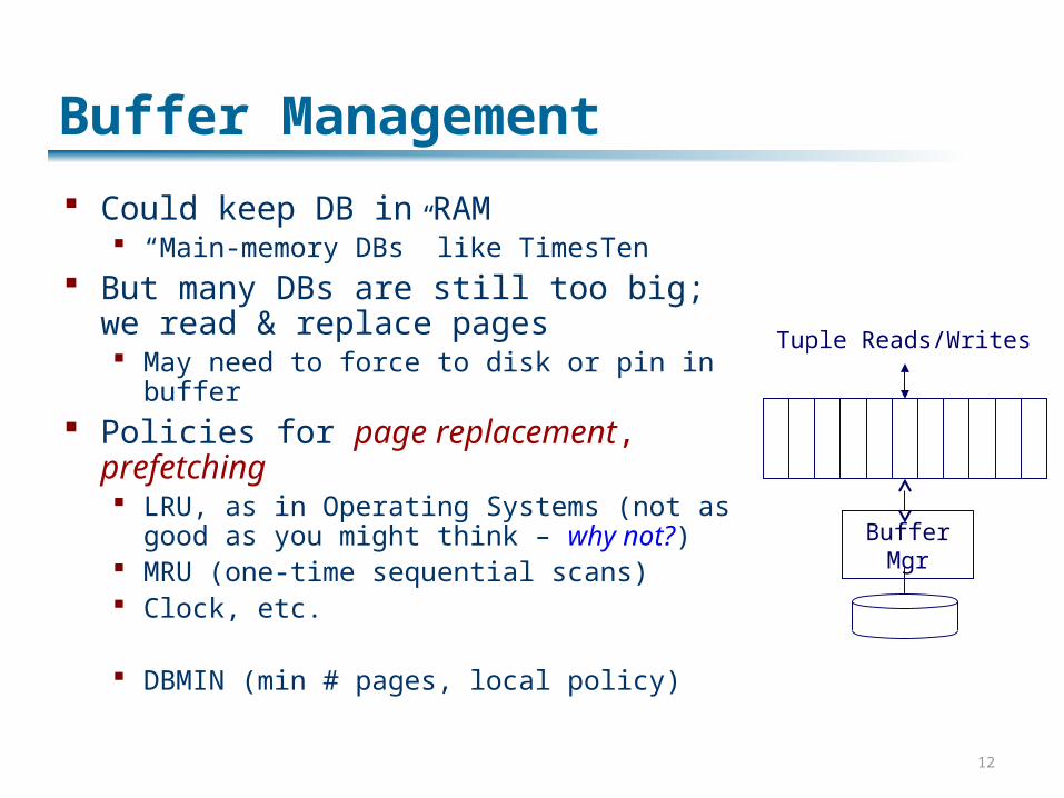
Buffer Management

Could keep DB in RAM “Main-memory DBs” like TimesTen

But many DBs are still too big; we read & replace pages May need to force to disk or pin in buffer

Policies for page replacement, prefetching LRU, as in Operating Systems (not as

good as you might think – why not?) MRU (one-time sequential scans) Clock, etc.

DBMIN (min # pages, local policy)

Buffer Mgr

Tuple Reads/Writes

13

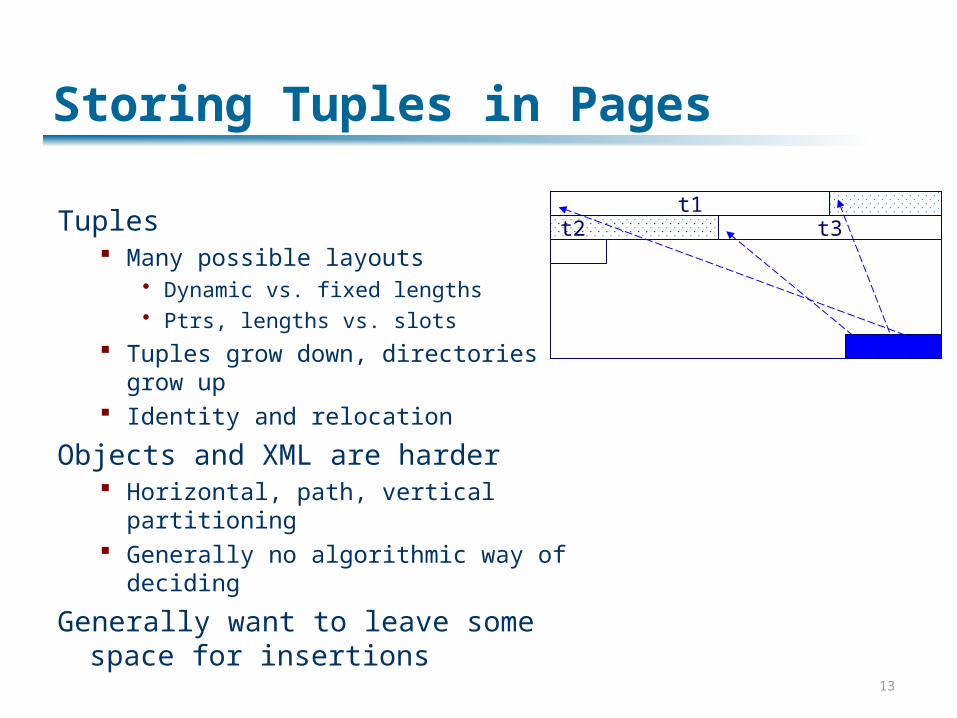
Storing Tuples in Pages

Tuples Many possible layouts

Dynamic vs. fixed lengths Ptrs, lengths vs. slots

Tuples grow down, directories grow up

Identity and relocation

Objects and XML are harder Horizontal, path, vertical partitioning Generally no algorithmic way of

deciding

Generally want to leave some space for insertions

t1t2 t3

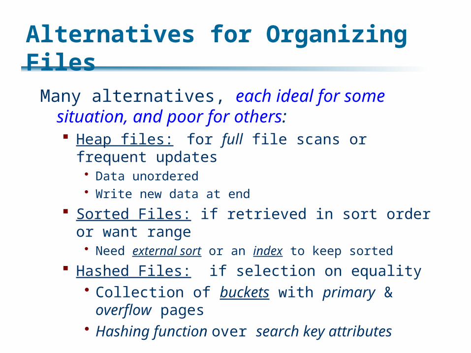
Alternatives for Organizing Files

Many alternatives, each ideal for some situation, and poor for others: Heap files: for full file scans or frequent

updates Data unordered Write new data at end

Sorted Files: if retrieved in sort order or want range Need external sort or an index to keep sorted

Hashed Files: if selection on equality Collection of buckets with primary & overflow

pages Hashing function over search key attributes

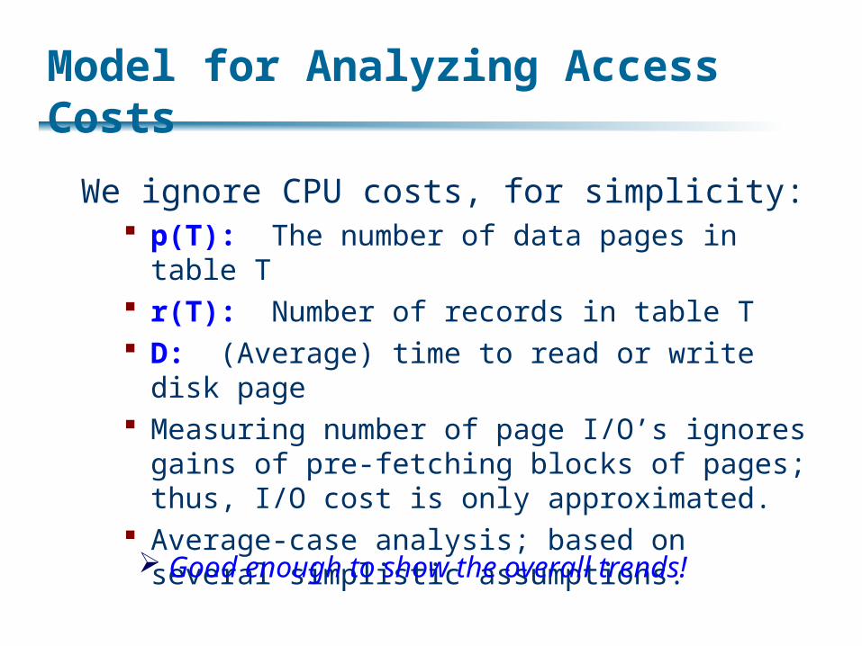
Model for Analyzing Access Costs

We ignore CPU costs, for simplicity: p(T): The number of data pages in table T r(T): Number of records in table T D: (Average) time to read or write disk page Measuring number of page I/O’s ignores gains

of pre-fetching blocks of pages; thus, I/O cost is only approximated.

Average-case analysis; based on several simplistic assumptions.

Good enough to show the overall trends!

Assumptions in Our Analysis

Single record insert and delete Heap files:

Equality selection on key; exactly one match Insert always at end of file

Sorted files: Files compacted after deletions Selections on sort field(s)

Hashed files: No overflow buckets, 80% page occupancy

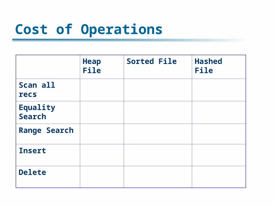
Cost of Operations

Heap File

Sorted File Hashed File

Scan all recs

Equality Search

Range Search

Insert

Delete

18

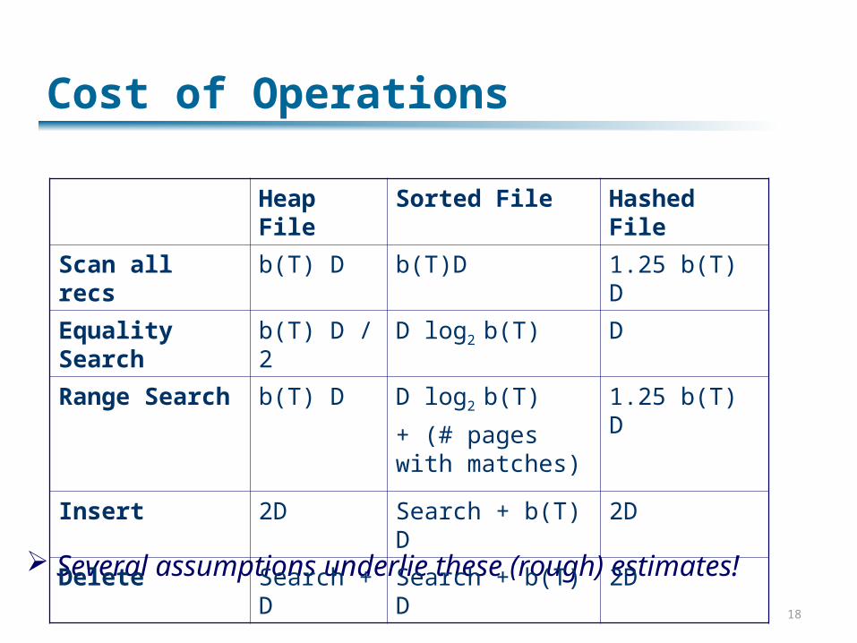
Several assumptions underlie these (rough) estimates!

Heap File

Sorted File Hashed File

Scan all recs b(T) D b(T)D 1.25 b(T) D

Equality Search

b(T) D / 2 D log2 b(T) D

Range Search

b(T) D D log2 b(T)

+ (# pages with matches)

1.25 b(T) D

Insert 2D Search + b(T) D 2D

Delete Search + D

Search + b(T) D 2D

Cost of Operations

19

Speeding Operations over Data

Three general data organization techniques: Indexing Sorting Hashing

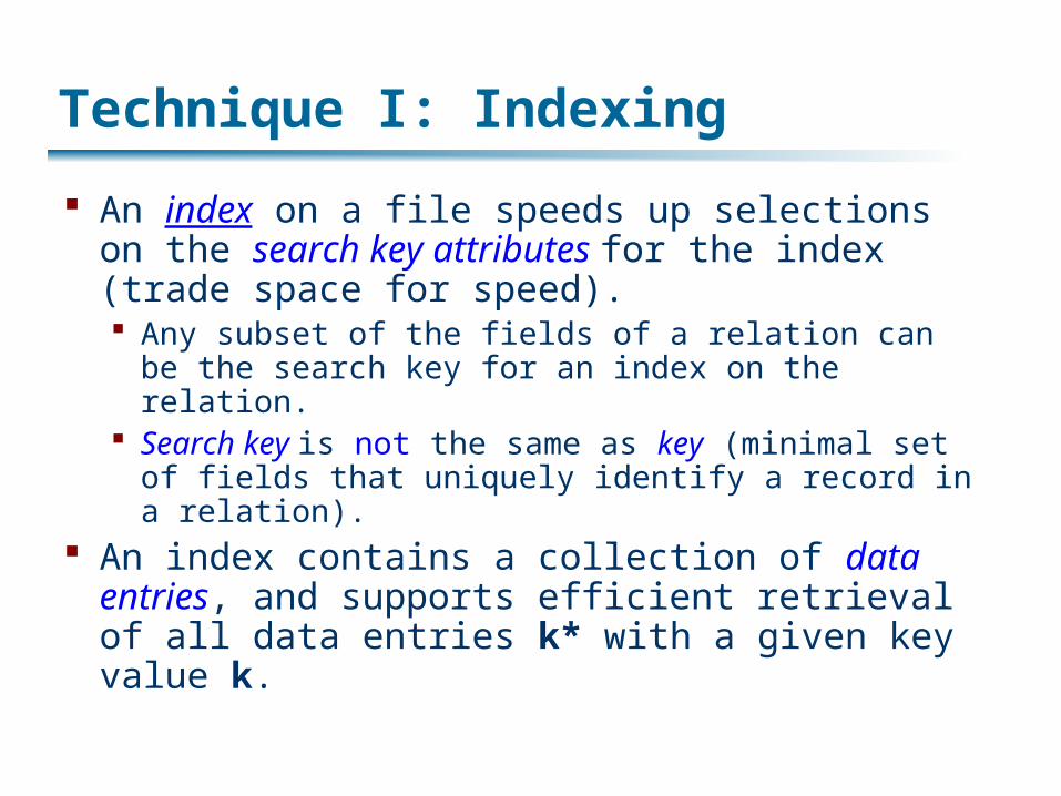
Technique I: Indexing

An index on a file speeds up selections on the search key attributes for the index (trade space for speed). Any subset of the fields of a relation can be the

search key for an index on the relation. Search key is not the same as key (minimal set

of fields that uniquely identify a record in a relation).

An index contains a collection of data entries, and supports efficient retrieval of all data entries k* with a given key value k.

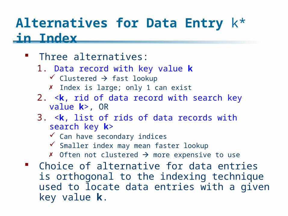
Alternatives for Data Entry k* in Index

Three alternatives:1. Data record with key value k

Clustered fast lookup Index is large; only 1 can exist

2. <k, rid of data record with search key value k>, OR

3. <k, list of rids of data records with search key k> Can have secondary indices Smaller index may mean faster lookup Often not clustered more expensive to use

Choice of alternative for data entries is orthogonal to the indexing technique used to locate data entries with a given key value k.

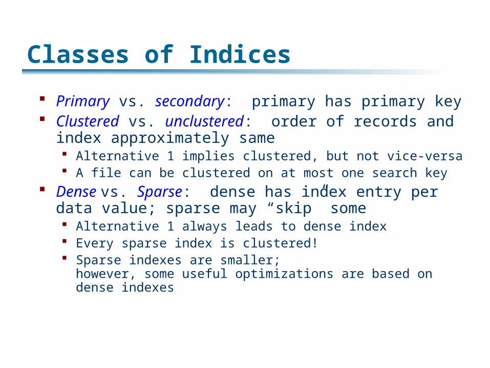
Classes of Indices

Primary vs. secondary: primary has primary key Clustered vs. unclustered: order of records and

index approximately same Alternative 1 implies clustered, but not vice-versa A file can be clustered on at most one search key

Dense vs. Sparse: dense has index entry per data value; sparse may “skip” some Alternative 1 always leads to dense index Every sparse index is clustered! Sparse indexes are smaller;

however, some useful optimizations are based on dense indexes

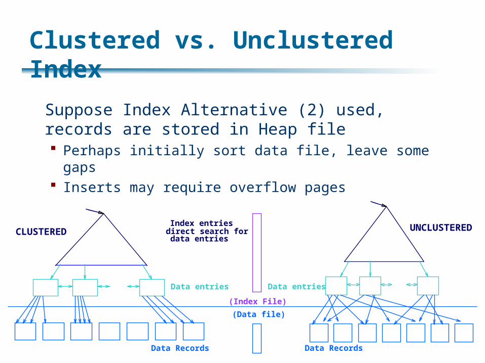
Clustered vs. Unclustered Index

Suppose Index Alternative (2) used, records are stored in Heap file Perhaps initially sort data file, leave some gaps Inserts may require overflow pages

Index entries

Data entries

direct search for

(Index File)

(Data file)

Data Records

data entries

Data entries

Data Records

CLUSTERED UNCLUSTERED

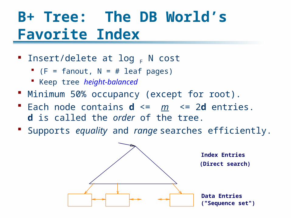
B+ Tree: The DB World’s Favorite Index

Insert/delete at log F N cost (F = fanout, N = # leaf pages) Keep tree height-balanced

Minimum 50% occupancy (except for root). Each node contains d <= m <= 2d entries.

d is called the order of the tree. Supports equality and range searches efficiently.

Index Entries

Data Entries("Sequence set")

(Direct search)

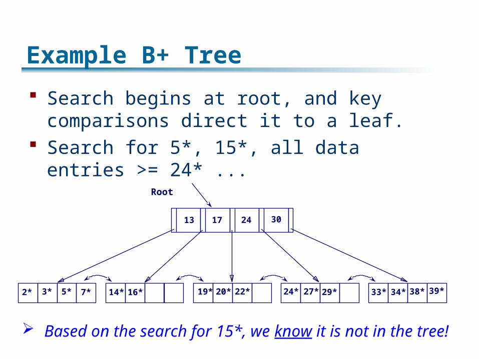
Example B+ Tree

Search begins at root, and key comparisons direct it to a leaf.

Search for 5*, 15*, all data entries >= 24* ...

Based on the search for 15*, we know it is not in the tree!

Root

17 24 30

2* 3* 5* 7* 14* 16* 19* 20* 22* 24* 27* 29* 33* 34* 38* 39*

13

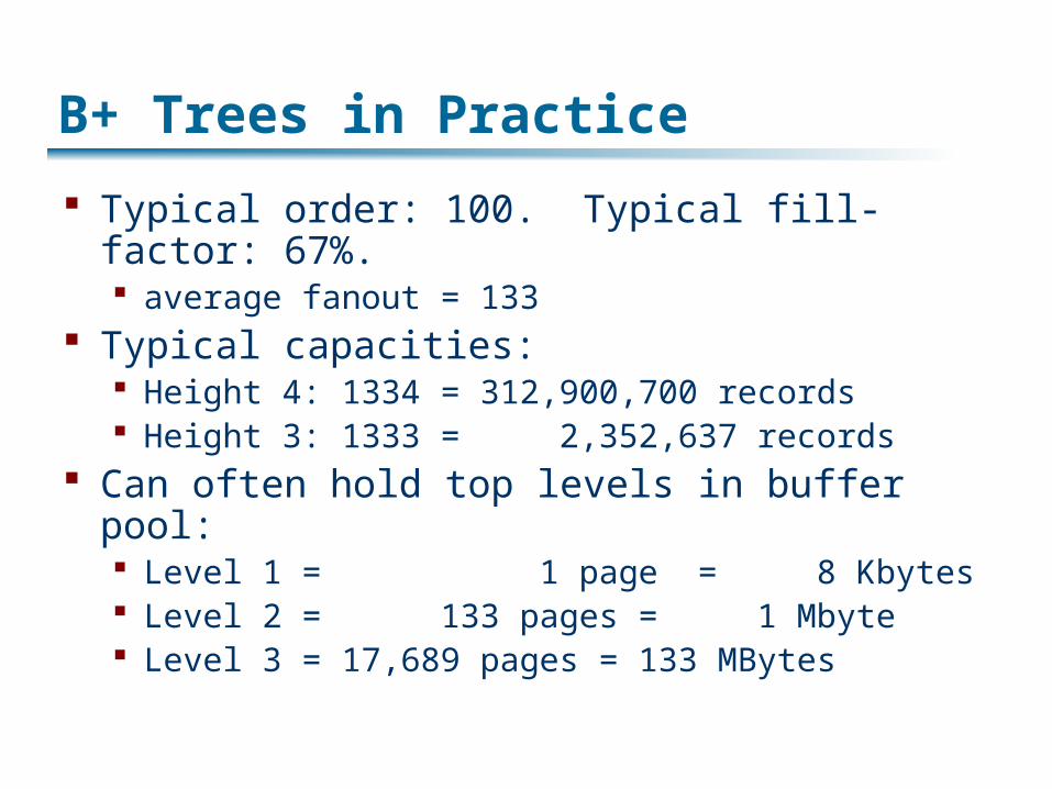
B+ Trees in Practice

Typical order: 100. Typical fill-factor: 67%. average fanout = 133

Typical capacities: Height 4: 1334 = 312,900,700 records Height 3: 1333 = 2,352,637 records

Can often hold top levels in buffer pool: Level 1 = 1 page = 8 Kbytes Level 2 = 133 pages = 1 Mbyte Level 3 = 17,689 pages = 133 MBytes

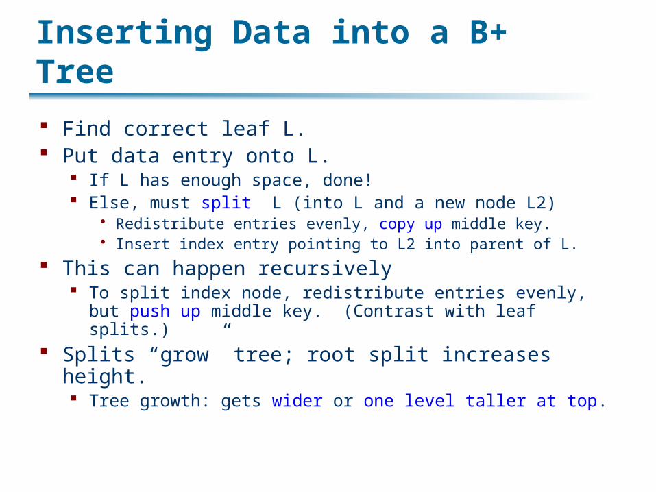
Inserting Data into a B+ Tree

Find correct leaf L. Put data entry onto L.

If L has enough space, done! Else, must split L (into L and a new node L2)

Redistribute entries evenly, copy up middle key. Insert index entry pointing to L2 into parent of L.

This can happen recursively To split index node, redistribute entries evenly, but push

up middle key. (Contrast with leaf splits.) Splits “grow” tree; root split increases height.

Tree growth: gets wider or one level taller at top.

Inserting 8* into Example B+ Tree Observe how minimum occupancy is

guaranteed in both leaf and index pg splits.

Recall that all data items are in leaves, and partition values for keys are in intermediate nodesNote difference between copy-up and push-up.

29

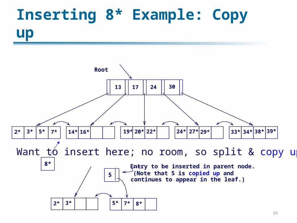
Inserting 8* Example: Copy up

Root

17 24 30

2* 3* 5* 7* 14* 16* 19* 20* 22* 24* 27* 29* 33* 34* 38* 39*

13

Want to insert here; no room, so split & copy up:

2* 3* 5* 7* 8*

5

Entry to be inserted in parent node.(Note that 5 is copied up andcontinues to appear in the leaf.)

8*

30

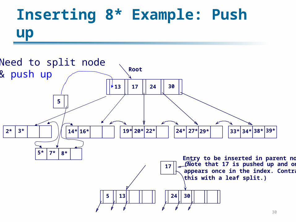
Inserting 8* Example: Push up

Root

17 24 30

2* 3* 14* 16* 19* 20* 22* 24* 27* 29* 33* 34* 38* 39*

13

5* 7* 8*

5

Need to split node & push up

5 24 30

17

13

Entry to be inserted in parent node.(Note that 17 is pushed up and onlyappears once in the index. Contrastthis with a leaf split.)

Deleting Data from a B+ Tree

Start at root, find leaf L where entry belongs. Remove the entry.

If L is at least half-full, done! If L has only d-1 entries,

Try to re-distribute, borrowing from sibling (adjacent node with same parent as L).

If re-distribution fails, merge L and sibling.

If merge occurred, must delete entry (pointing to L or sibling) from parent of L.

Merge could propagate to root, decreasing height.

B+ Tree Summary

B+ tree and other indices ideal for range searches, good for equality searches. Inserts/deletes leave tree height-balanced; logF N cost.

High fanout (F) means depth rarely more than 3 or 4. Almost always better than maintaining a sorted file. Typically, 67% occupancy on average. Note: Order (d) concept replaced by physical space

criterion in practice (“at least half-full”). Records may be variable sized Index pages typically hold more entries than leaves

33

Other Kinds of Indices

Multidimensional indices R-trees, kD-trees, …

Text indices Inverted indices

Structural indices Object indices: access support relations, path

indices XML and graph indices: dataguides, 1-indices,

d(k) indices

34

DataGuides (McHugh, Goldman, Widom)

Idea: create a summary graph structure representing all possible paths through the XML tree or graph A deterministic finite state machine representing

all paths Vaguely like the DTD graph from the

Shanmugasundaram et al. paper

At each node in the DataGuide, include an extent structure that points to all nodes in the original tree These are the nodes that match the path

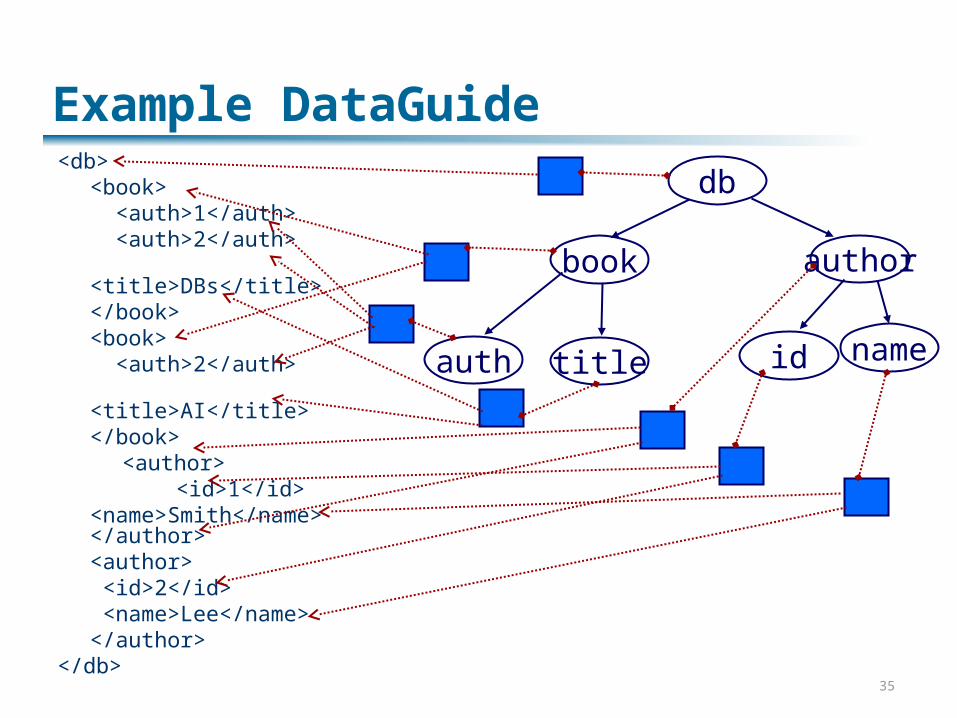
35

Example DataGuide<db>

<book> <auth>1</auth> <auth>2</auth> <title>DBs</title></book><book> <auth>2</auth> <title>AI</title></book>

<author> <id>1</id>

<name>Smith</name></author><author> <id>2</id> <name>Lee</name></author>

</db>

db

authorbook

title nameidauth