Under What Assumptions do Site­by­Treatment Instruments 

Identify Average Causal Effects? 

 

sean f. reardon Stanford University 

  

Stephen W. Raudenbush University  f Chicago o

 

 

 

Draft November 2, 2010 

 

         Direct correspondence to Sean F. Reardon (sean.reardon@stanford.edu).  This work was supported by a grant from the Institute for Education Sciences (R305D090009), and 

Howard Bloom, Fatih Unlu, Pei benefitted enormously from lengthy conversations with Zhu, and Pamela Morris.  All errors are our own.    

ABSTRACT 

The increasing availability of data from multi‐site randomized trials provides a 

potential opportunity to use instrumental variables methods to study the impacts of 

multiple hypothesized mediators of the effect of a treatment.  We describe nine 

assumptions needed to identify the impacts of multiple mediators when using site‐by‐

treatment interactions to generate multiple instruments.  Three of these assumptions are 

unique to the multiple‐site, multiple‐mediator case: 1) the assumption that the mediators 

act in parallel (no mediator affects another mediator); 2) the assumption that the site‐

average effect of the treatment on each mediator is independent of the site‐average effect 

of each mediator on the outcome; and 3) the assumption that the site‐by‐compliance 

matrix has sufficient rank.  The first two of these assumptions are non‐trivial and cannot be 

empirically verified, suggesting that multiple‐site, multiple‐mediator instrumental 

variables models must be justified by strong theory.  

 

1

1. INTRODUCTION 

  In canonical applications of the instrumental variable method, exogenously 

determined exposure to an instrument (such as random assignment to a treatment 

condition) induces exposure to a mediating process that in turn causes a change in a later 

outcome.  A crucial assumption known as the exclusion restriction is that the hypothesized 

instrument can influence the outcome only through its influence on exposure to the 

mediator of interest (Heckman & Robb, 1985b; Imbens & Angrist, 1994). It may be the case, 

however, that multiple mediators operate jointly to influence the outcome, in which case a 

ingle is nstrument will not suffice to identify the causal effects of interest.  

  To cope with this problem, analysts have recently exploited the fact that a causal 

process is often replicated across multiple sites, generating the possibility of multiple 

instruments in the form of site‐by‐instrument interactions.  These multiple instruments 

can, in principle, enable the investigator to identify the impact of multiple processes 

regarded as the mediators of the effect of a treatment (or, equivalently, of multiple 

programs or treatments regarded as the mediators of the effect of an instrument).  Kling, 

Liebman, and Katz (2007), for example, used random assignment in the Moving to 

Opportunity (MTO) study as an instrument to estimate the impact of neighborhood poverty 

on health, social behavior, education, and economic self‐sufficiency of adolescents and 

adults.  Reasoning that the instrument might affect outcomes through mechanisms other 

than neighborhood poverty, they control for a second mediator, use of the randomized 

treatment voucher.  To do so, they capitalize on the replication of the MTO experiment in 

2

five cities, generating ten1 instruments (“site‐by‐randomization interactions”) to identify 

the impact of the two mediators of interest, neighborhood poverty and experimental 

compliance.  Using a similar strategy, Duncan, Morris, and Rodrigues (forthcoming) use 

data from 16 implementations of welfare‐to‐work experiments to identify the impact of 

family income, average hours worked, and receipt of welfare as mediators.  

Clearly, this strategy for generating multiple instruments has potentially great 

appeal in research on causal effects in social science.  For example, Spybrook (2008) found 

that, among 75 large‐scale experiments funded by the US Institute of Education Sciences 

over the past decade, the majority were multi‐site studies in which randomization occurred 

within sites.  In principle, these data could yield a wealth of new knowledge about causal 

effects in education policy.  It is essential, however, that researchers understand the 

assumptions required to pursue this strategy successfully.  To date, we know of no 

complete account of these assumptions. 

  Our purpose therefore is to clarify the assumptions that must be met if this 

“multiple site, multiple mediator” instrumental variables strategy (hereafter MSMM‐IV) is 

to identify the average causal effects (ATE) in the populations of interest.  For simplicity of 

exposition, and corresponding to the applications of MSMM‐IV to date, we consider the 

case of where a single treatment   operates through a set of mediators 

, , … , , which are linearly related to an outcome  .  We conclude that, in 

addition to the assumptions typically required in the single‐site, single‐instrument, single‐

mediator case, three additional assumptions are required in the MSMM‐IV case.  

1 The five sites generate ten site‐by‐treatment interactions as instruments because there were three 

(randomly assigned) treatment conditions per site.

3

  We begin by delineating the assumptions required for identification in the case of a 

single instrument and a single mediator within a single‐site study.  Unlike Angrist, Imbens, 

and Rubin (1996) (AIR), we consider the general case where both the treatment and the 

mediator may be continuous or multi‐valued.  In this general case, the assumptions 

required for identification of the average treatment effect differ somewhat from those AIR 

(1996) describe for the binary treatment and binary mediator case.  We link our discussion 

to recent papers describing the correlated random coefficient (CRC) model, and show that 

the average treatment effect in the CRC model is identified by instrumental variables using 

a weaker assumption than that described by Heckman and Vytlacil (1998) and Wooldridge 

(2003).   

  Following a discussion of the single, site, single mediator case, we then consider the 

case of multiple sites with a single mediator, delineating the assumptions required in this 

case.  We then turn our attention to the case of primary interest: the MSMM‐IV design.  We 

specify a set of nine assumptions required for the MSMM‐IV model to identify the average 

treatment effects of the mediators, three of which are specific to the MSMM‐IV case, and 

hich we discuss in some detail.  w

 

2. THE SINGLE‐SITE, SINGLE‐MEDIATOR CASE 

  Suppose that each participant in a single‐site study is exposed to an instrument   

taking on values in the domain  .  We often consider instruments taking on values in 

the domain  0,1 , where  1 if the individual is assigned to the “treatment” condition 

or  0 if the participant is assigned to the alternative “control” condition.  More 

generally, however,   may be multi‐valued or continuous. 

4

  In order to define a set of causal estimands of interest, we require the assumption 

that an individual’s potential outcomes depend only on the treatment condition and 

mediator conditions to which that particular individual is exposed (and not on the 

treatment and mediator conditions of others), known as the Stable Unit Treatment Value 

Assumption (SUTVA) (Rubin, 1986).  In the standard potential outcomes framework, we 

typically require a single SUTVA assumption stating that one individual’s potential 

outcomes do not depend on others’ treatment status.  In the IV model, however, the 

presence of three variables of interest—the treatment  , a mediator  , and an outcome 

—necessitates a pair of such assumptions (Angrist et al., 1996), stated formally below.  

 

Ass onumpti  (i): Stable unit treatment value assumptions (SUTVA):  

(i.a)   Each unit   has one and only one potential value of the mediator   for each 

treatment condition  : that is, for a population of size  ,  , , … ,

 for all  1,2, … , . 

(i.b)  Each unit   has one and only one potential outcome value of   for each pair of 

values of treatment condition   and mediator value  : that is, for a population of 

ize  ,  , , … , , , , … , ,  for all  1,2, … , . s

 

Given the SUTVA assumptions, we can represent the potential outcome   for a participant 

who experiences treatment   and mediator value   as  ,  (we drop the subscript 

 throughout the remainder of this paper except when necessary for clarity).  Our second 

assumption is that   affects   only through its impact on the mediator,  . This is the 

standard exclusion restriction assumption: 

5

 

Assumption (ii): Exclusion restriction: 

, . 

 

The exclusion restriction combined with the second SUTVA assumption (i.b) implies a third 

SUTVA condition: (i.c) Each unit   has one and only one potential outcome value of   for 

each value of the mediator  : that is, for a population of size  ,  , , … ,  

for all  1,2, … , . 

The SUTVA assumptions are necessary in order to define the causal estimands of 

interest.  If the treatment variable is binary, for example, the first SUTVA assumption (i.a) 

implies that we can define the person‐specific casual effect of the treatment on   as 

Γ 1 0 .2  If, however, the treatment is not binary, it will be useful to assume that 

he person‐specific effect of   on   is linear in  , in which case Γ 1 : t

 

Assumption (iii): Person­specific linearity of the mediator   in  : The person‐specific effect 

f   on mediator   is linear.  That is,  0 Γ. o

 

Likewise, it will be useful to assume that the person‐specific effect of   on   is 

linear in  .  In this case, the third SUTVA condition (i.c) implies that we can define the 

2 Note that if both   and   are binary, taking on values of 0 or 1, then Γ 1,0,1 .  In this case, Angrist, 

Imbens, and Rubin (Angrist et al., 1996) assume that there do not exist both individuals for whom Γ 1 and 

individuals for whom Γ 1 (this is the no “defiers” assumption, in their terminology; also called the 

monotonicity assumption).  We will not require the monotonicity assumption, for reasons we discuss below. 

6

person‐specific casual effect of the mediator  as Δ 1 :   

  Assumption (iv): Person­specific linearity in  : the person‐specific effect of the mediator 

 on   is linear.  That is,  0 Δ. 

 

The combination of (ii), (iii), and (iv) implies that the person‐specific effect of   on   is 

linear in  : 

0 Γ  

0 0 Γ Δ 

0 0 Δ ΓΔ 

Thus, defining Β as the person‐specific effect of   on  , we can relate the person‐specific 

   by effects of   on   and of   on   to the person‐specific effect of   on

(1)   1 Β ΓΔ. 

Let us define the population average intent‐to‐treat effect (ITT) of interest here as 

Β . Similarly, the average causal effect of   on the mediator   (the “average 

compliance”) is  Γ ; and  Δ  is the average treatment effect (ATE) of   on  . 

This ATE is typically of central interest in studies using instrumental variables. Taking the 

xpectation of (1), we have   e

 

Β ΔΓ Δ, Γ .  (2)  

 

Two additional assumptions allow us to express the ATE as ratio of the ITT effect to the 

average compliance.  These are: 

7

   

Assumption (iv): No person­specific compliance­effect covariance:  Δ, Γ 0. 

 

Assumption (v): Effectiveness of the instrument:  0. 

 

The no compliance‐effect covariance assumption means that the extent to which treatment 

status affects an individual’s value of the mediator   is uncorrelated with the extent to 

which   affects the indivudal’s outcome  .  This may not always be a plausible assumption.  

For example, if individuals have some knowledge of how much they will benefit from an 

intervention, those for whom the intervention is most effective may comply more fully with 

it, if offered it, than those for whom the intervention is less effective.  

  The instrument effectiveness assumption simply means that the average effect of 

the treatment on the mediator is non‐zero (though the effect may be positive for some 

individuals and negative for others).  Together, these two assumptions enable us to write 

Equation (2) as 

,     0. 

  (3) 

The six assumptions derived so far enable us to equate the ATE to the ratio  / .  

The parameters   and   are not directly observable, however, because they are means of 

differences in counterfactual outcomes.  If we are willing to assume that persons are 

assigned ignorably to treatments   for  , as would be true in a randomized 

experiment, we can identify (3) from sample data.  We therefore add our seventh and final 

8

assumption in this section:  

 

Assumption (vii):  Ignorable treatment assignment:   , , .  

 

Applying the no‐compliance‐effect assumption (v) and ignorable treatment assignment 

(vii), we can equate the ITT effect (2) to the estimable quantity  | |

, yielding 1

 

| | 1 | 1 | 1    

                        1           (vii)                               

             1  

                        Β Δ, Γ      

                      .              (v)     

)   (4

  Without the no compliance‐effect‐covariance assumption (v), but allowing all other 

ssumptions, the instrumental variable estimand in a population of size   is  a

 

Δ, Γ Δ, Γ ∑ Γ Δ∑ Γ

. 

  (5) 

 

Equation (5) may be regarded as a “compliance‐weighted average treatment effect” 

(CWATE) because each person’s treatment effect Δ is weighted by his or her compliance, Γ.  

9

The magnitude of the bias in the CWATE relative to the ATE is determined not only by the 

covariance of Γ and Δ, but also by the inverse of  .  When   is small, any bias due to 

compliance‐effect covariance will be exacerbated. 

Heckman and colleagues have argued that this CWATE may not be an economically 

or policy relevant parameter, in part because it is dependent on the specific instrument 

that induces exposure to the mediator (Heckman & Robb, 1985a, 1986; Heckman, Urzua, & 

Vytlacil, 2006).  Because Γ is instrument‐specific, the IV estimand in this case is likewise 

nstrument‐specific when the no compliance‐effect covariance assumption fails. i

 

The Case of Binary   and   

Angrist, Imbens, and Rubin (1996) consider the case where both   and   are 

binary.  In this case, the population may contain at most four types of individuals: 

“compliers,” for whom Γ 1 0 1 0 1; “never‐takers,” for whom 

Γ 0 0 0; “always‐takers,” for whom Γ 1 1 0; and “defiers,” for whom 

0 1 1.  The monotonicity or “no defiers” assumption,  Γ

 

1 0 ,      1, … , 

 

eliminates the possibility of defiers.  Under this assumption, we can simplify the expression 

or the CWATE of (5) to  f

 

∑ ΔΔ|Γ 1  

10

  (6)

where   is the number of compliers in the population.  Angrist and Imbens (1996) termed 

 the “local average treatment effect” (LATE), also known as the average treatment effect 

on the compliers or the complier average treatment effect (CATE).  Equation (6) shows that 

the LATE is a special case of the CWATE when both   and   are binary and the montonicity 

assumption holds.  Angrist, Imbens, and Rubin (1996) did not note the no compliance‐

effect c 3 

 

ovariance assumption (iv) because it is not required to obtain the LATE.

Note, however, that monotonicity is not an assumption required for the 

identification of the ATE parameter  .  If there are defiers (or more generally, if there are 

both individuals for whom Γ 0 and individuals for whom Γ 0), Equation (5) plus the 

ssumptions that  Γ, Δ 0 and  0 ensure that a . 

 

The Correlated Random Coefficients Model 

  Above we note that the assumption that the no compliance‐effect covariance 

assumption is necessary for instrumental variables estimators to identify the average 

treatment effect in the population.  We digress here briefly to relate this assumption to the 

specific application of the instrumental variables model in the case of the correlated 

random coefficients (CRC) model discussed by Heckman and Vytlacil (1998) and 

Wooldridge (2003).  In the CRC model, the effect Δ of a causal variable   on an observable 

outcome   varies across individuals, as in the model  

3 In some settings (e.g., Little & Yau, 1998), participants assigned to the control cannot gain access to the 

mediator, that is Pr 0 0 1.0. In this case, there are no “always‐takers.” We then see that LATE 

becomes the “treatment effect on the treated” (TOT), that is  Δ| 1 . 

11

Δ

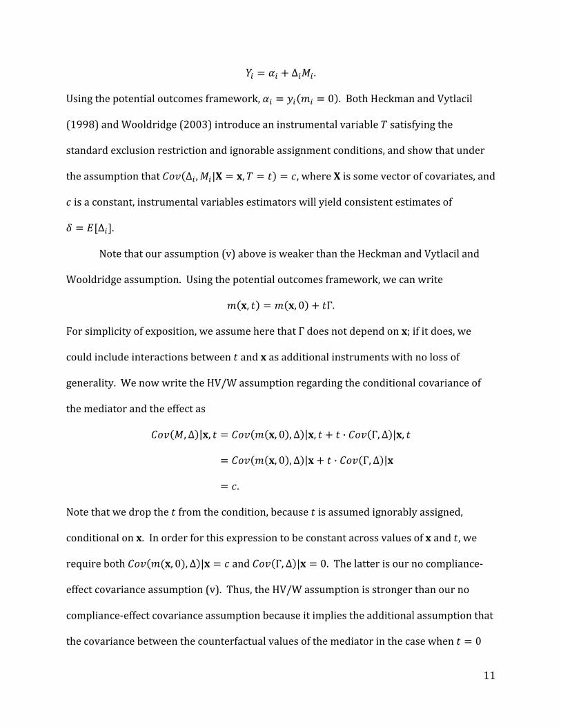
Using the potential outcomes framework,  0 .  Both Heckman and Vytlacil 

(1998) and Wooldridge (2003) introduce an instrumental variable   satisfying the 

standard exclusion restriction and ignorable assignment conditions, and show that under 

the assumption that  Δ , | , , where   is some vector of covariates, and 

 is a constant, instrumental variables estimators will yield consistent estimates of 

Δ

. 

. 

Note that our assumption (v) above is weaker than the Heckman and Vytlacil and 

Wooldridge assumption.  Using the t mework, we can write   poten ial outcomes fra

, , 0 Γ. 

For simplicity of exposition, we assume here that Γ does not depend on  ; if it does, we 

could include interactions between   and   as additional instruments with no loss of 

generality.  We now write the HV/W assumption regarding the conditional covariance of 

the mediator and the effect as 

, Δ | , , 0 , Δ | , · Γ, Δ | ,  

, 0 , Δ | · Γ, Δ |  

. 

Note that we drop the   from the condition, because   is assumed ignorably assigned, 

conditional on  .  In order for this expression to be constant across values of   and  , we 

require both  , 0 , Δ |  and  Γ, Δ | 0.  The latter is our no compliance‐

effect covariance assumption (v).  Thus, the HV/W assumption is stronger than our no 

compliance‐effect covariance assumption because it implies the additional assumption that 

the covariance between the counterfactual values of the mediator in the case when  0 

12

and the effect of the mediator is constant across values of  .  However, our result above 

demonstrates that the we require only that  Γ, Δ | 0; it is not necessary that 

, 0 , Δ |  be constant across values of  . 

Our formulation above clarifies that IV estimators rely on an assumption regarding 

the relationship between the effects of the instrument on the mediator and the effects of 

the mediators on the outcomes, not an assumption about the relationship between the 

observed levels of the mediator and its effects.  This is because the IV model relies for 

identification on the fact that the instrument induces some exogenous variation in the 

mediator; the amount of this variation must be independent of the effects of the mediator 

in order to avoid bias in the IV estimator.  By focusing on the relationship between the 

observed values of the mediator and its (unobserved) effects, Heckman and Vytlacil (1998) 

and Woolridge (2003) make a stronger assumption than is necessary.  A correlation 

between the observed values of a mediator and its effects that arises solely from a 

correlation between baseline levels of the mediator and its effects will not cause bias in the 

instrumental variables estimates. 

 

Summary of Single­Site, Single Mediator IV Assumptions 

  Approaching the instrumental variable model from a potential outcomes framework 

is particularly useful when we allow treatment effects to be heterogeneous. After imposing 

assumptions (i)‐(iv) (SUTVA, exclusion restriction, and linearity), this framework reveals 

the importance of (v), the no‐compliance‐effect‐covariance assumption along with the 

conventional assumptions (vi) and (vii) (effectiveness of the instrument and ignorable 

treatment assignment). If (v) fails, the instrumental variable estimand is a compliance 

13

weighted average treatment effect (CWATE): those persons whose mediator is most 

affected by the instrument will be assigned the greatest weight in the estimand.  In the case 

of a binary instrument and binary mediator, we can replace the “no compliance‐covariance 

assumption” with a monotonicity assumption; in this case CWATE=LATE, the local average 

treatment effect.  In addition, if the members of the control group can be assumed to have a 

nown and constant value of the mediator, LATE=TOT, the treatment effect on the treated.   k

 

3. THE IV MODEL WITH MULTIPLE SITES AND A SINGLE MEDIATOR 

We next consider the case of a multi‐site study, where within each site each 

participant is exposed to an instrument  , which may influence   through a single mediator 

.  In this case, if we accept that assumptions (i)‐(iv) (SUTVA, exclusion restriction, and 

inearity) hold within each site, we can write Equation (2) as l

 

Β| ΔΓ| Δ, Γ , 

  (7

where   indexes sites and where  Δ|  and  Γ| .  Pooling (7) across 

ites, we have 

) 

s

 

Β Δ, Γ  

, Δ, Γ . 

  (8)

Now, rather than the single assumption that  Δ, Γ 0, we need two compliance‐effect 

covariance assumptions: 

 

14

 

Assumption (v.a): No average within­site compliance­effect covariance:  Δ, Γ 0.  A 

simpler, but stronger assumption, is that there is no within‐site compliance‐effect 

covariance in any site:  Δ, Γ 0 for all  . 

Assumption (v.b): No between­site compliance effect covariance:  , 0.  

 

These assumptions, together with assumption (vi) (instrument effectiveness), enable us to 

rite (8) as  w

 

,      0, 

  (3

as above.  Assumption (vii) (ignorable treatment assignment within sites) then enables us 

o identify the causal effect   from sample data.  

) 

t

 

4. THE IV MODEL WITH MULTIPLE SITES AND MULTIPLE MEDIATORS 

We now consider the case of particular interest for this paper, the case where 

subjects within a multi‐site study are exposed to a treatment  , which may influence   

through   distinct mediators  , , … .  We first assume that both SUTVA assumptions 

hold (i.a and i.b)) with respect to the vector of   mediators:   

 

Assump i)tion ( : Stable unit treatment value assumptions (SUTVA):  

(i.a)   Each unit   has one and only one potential value of the vector of mediators 

15

, , … ,  for each treatment condition  : that is, for a 

population of size  ,  , , … ,  for all  1,2, … , . 

(i.b)   Each unit   has one and only one potential outcome value of   for each 

treatment condition   and each vector of mediator values  : that is, for a 

population of size  ,  , , … , , , , … , ,  for all 

1,2, … , . 

 

We next assume that assignment to   influences   only through the list of   distinct 

and observable mediators  , , … .  Specifically, each participant has potential 

mediator values  , , … ,  for  .  The exclusion restriction now requires 

that   affects   only through its effects on one or more of the mediators.  That is: 

 

Assumption (ii): Exclusion restriction: The treatment   affects   only through its impact on 

the set of   mediators,  , , … , .  That is,  , . 

 

As above, we also assume person‐specific linearity of each   in   (iii) and linearity of   in 

each of the mediators (iv).  Specifically, we assume that the outcome   is a linear function 

f the mediators, and that there are no interactions among the mediators. o

 

Assumption (iii): Person­specific linearity of each mediator in  : The person‐specific effect of 

 on each mediator   is linear.  That is,  0 Γ  for each  . 

Assumption (iv): Person­specific linearity of   in  : The person‐specific effect of each 

mediator   on   is linear.  That is,  ∑ Δ . 

16

 

These imply, respectively, that the person‐specific causal effect of   on   is Γ

1 , and that that the person‐specific causal effect of   on   is Δ

1 , for all  1,2, … , .  As above, the person‐specific causal effect of   on   is 

Β 1 .  The observed outcome is    0  Β. 

We next assume that assignment to   does not influence a given mediator   

through any other mediator  .  That is, the mediators do not influence one another.  This 

is required so that the estimation of the effects of a given mediator   on   are not 

confounded with the effects of another mediator  . 

 

Assumption (v l): Paralle  mediators:  

, , … , , , … ,   for all  1,2, , … , . 

 

ogether, the five assumptions above define the person‐specific intent‐to‐treat effect as T

 

Β 1  

, , … , 1 , 1 , … , 1  

Δ Γ . 

  (9

Equation (9) says that the person‐specific effect of   on   can be written as the sum of the 

products of the person‐specific effects of   on each mediator and the person‐specific effects 

of that mediator on the   (below we discuss the implications of a failure of the parallel 

) 

17

mediator assumption).  Taking the expectation of (9) over the population within a site   

ields y

 

Β| Δ Γ | Δ , Γ , 

  (10

where   and   are the average effect of   on   in site   and the average effect of   on 

 in site  , respectively; and where  Δ , Γ  is the covariance between Δ  and Γ  in 

ite  . 

) 

s

  We next assume no within‐site covariance between Δ  and Γ  for each mediator  :  

 

Assumption (vi): No within­  compliance­effecsite t covariance:  

    Δ , Γ 0, for all   and  . 

 

e now have, for each site  , the equation W

 

 

 

, 

  (11) 

18

w  is the average, across sites, of the  ’s and  ∑ . 

  Equation (11) shows that, under the assumptions above, the site‐average  ’s can be 

expressed as a linear combination of the site‐average  ’s plus some site‐specific residual 

error term.  The coefficients   on the   terms are the parameters of interest—the 

average effects of the mediators on the outcome  .  Equation (11) suggests that the  ’s 

may be estimated with a multiple linear regression estimator, under the assumption that 

the errors have an expected value of zero, given the  ’s.  This insight suggests we require 

n assumption regarding the independence of the  ’s and  ’s: 

here 

a

 

Assumption (vii): Between­site compliance­effect independence: The site‐average compliance 

of each mediator is independent of the site‐average effect of each mediator.  That is, 

| , , … ,  for all  1, … , .   

 

Note that the assumption that the site‐mean compliance is independent of the site‐mean 

effect is stronger than an assumption of no compliance‐effect covariance (the latter 

requires only no linear association between compliance and effect; the former requires no 

association whatsoever).  Moreover, note that this assumption requires not only that there 

be no compliance‐effect association for a given mediator, but also that there be no cross‐

mediator compliance‐effect association.  That is, the site‐average effect of   on a given 

mediator   cannot be correlated with the site‐average effect of any mediator   on  . 

nder this assumption, we can write the expected value of the error   in (11) as  U

 

19

| , , … , , , … , 0 

· | , , … ,  

·  

0. 

 

In order that Equation (11) identify the  ’s, we must know  ’s and the  ’s.  Although 

these cannot be observed from the data, under the assumption of ignorable within‐site 

treatment assignment, each of the  ’s and the  ’s can be estimated from the sample data.  

hus, as above, we require: T

 

Assumption (viii): Ignorable within­site treatment assignment: The assignment of the 

instrument (the treatment, in our notation) must be independent of the potential outcomes 

ithin each site:  | , | ,   , 1, … , . w

 

Given the  ’s and the  ’s, we can estimate the  ’s, so long as the site‐by‐mediator 

ompliance matrix has sufficient rank.  We formalize this assumption below: c

 

Assumption (ix): Site­by­mediator compliance matrix has sufficient rank.  In particular, if   is 

the   x   matrix of the  , we require  .  This implies three specific 

conditions: 

20

(ix.a)  The compliance of at least  1 of the mediators varies across sites.  That is,  

0, for at most one  1,2, … , . 

(ix.b)  There are at least as many sites as mediators:  . 

(ix.c)  There is some subset of   site‐specific compliance vectors, 

, , … , , where  , that are linearly independent. 

 

The sufficient rank assumption is a generalization of the familiar instrument effectiveness 

assumption (assumption (vi) in the first section).  Note that when there is a single mediator 

( 1), the site‐by‐mediator compliance matrix will have rank 1 so long as  0 for at 

least one site   (the average compliance across sites may be zero, as long as it is not zero in 

every site).  Thus, when there is a single site and a single mediator, the sufficient rank 

assumption is therefore identical to the usual condition that the treatment have a non‐zero 

verage impact on the mediator.     a

 

5. DISCUSSION  

Summary of Multiple­Site, Multiple­Mediator IV Assumptions 

To summarize, in the case of a multi‐site study in which an treatment   may affect 

the outcome   through multiple mediators, we require a number of assumptions in order 

o identify the average causal effects of the mediators using MSSM‐IV methods.  These are: t

 

(i) Stable unit treatment value assumptions 

(ii) Exclusion restriction 

(iii) Person‐specific linearity of the mediators with respect to the treatment 

21

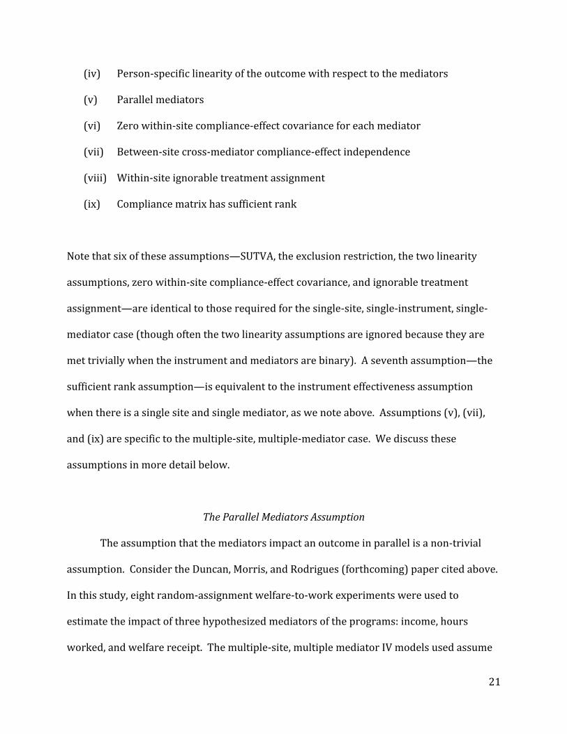
(iv) Person‐specific line arity of the outcome with respect to the mediators 

(v) Parallel mediators 

r(vi) Zero within‐site compliance‐effect covariance for each mediato

ect independence 

 

(vii) Between‐site cross‐mediator compliance‐eff

)(viii Within‐site ignorable treatment assign

(ix) ompliance matrix has sufficient rank 

ment 

C

 

Note that six of these assumptions—SUTVA, the exclusion restriction, the two linearity 

assumptions, zero within‐site compliance‐effect covariance, and ignorable treatment 

assignment—are identical to those required for the single‐site, single‐instrument, single‐

mediator case (though often the two linearity assumptions are ignored because they are 

met trivially when the instrument and mediators are binary).  A seventh assumption—the 

sufficient rank assumption—is equivalent to the instrument effectiveness assumption 

when there is a single site and single mediator, as we note above.  Assumptions (v), (vii), 

and (ix) are specific to the multiple‐site, multiple‐mediator case.  We discuss these 

ssumptions in more detail below. a

 

The Parallel Mediators Assumption 

The assumption that the mediators impact an outcome in parallel is a non‐trivial 

assumption.  Consider the Duncan, Morris, and Rodrigues (forthcoming) paper cited above.  

In this study, eight random‐assignment welfare‐to‐work experiments were used to 

estimate the impact of three hypothesized mediators of the programs: income, hours 

worked, and welfare receipt.  The multiple‐site, multiple mediator IV models used assume 

that the none of these mediators affects the others.  However, this is an implausible 

assump   tion, given that both hours worked and welfare receipt are clearly linked to income. 

For illustration, consider a simple case in which a treatment   affects   through two 

mediators,  1 and  2, one of which affects the other, as shown in the structural diagram 

below: 

Figure 1:

22

Let Γ  and Γ  be the person‐specific e ec 1 nd  2, respectively.  Note that  ff ts of   on   a

Γ Γ Γ Λ , 

where Γ  is the direct effect of   on  2 (the effect not mediated by  1), and Λ  is the 

effect of  1 on  2.  Likewise, let Δ  and Δ  be the effects of  1 and  2 on  , respectively.  

Note that  

Δ Δ Λ Δ , 

here Δ  is the direct effect of  1 on    he  fect not mediated by  2). w (t ef

  Now, the person-specific effect o is given by f on

Γ ΔB Γ Δ

Typically, we want to estimate Δ and Δ . Given a multi-site trial, within each

site , we have

| Γ Δ |   Γ Δ |    

Γ

Γ Δ

Λ

ΔM2

M1

T Y

23

Γ , Δ Γ , Δ  

Let us assume Γ , Δ 0 and Γ , Δ 0. The first of these says that the person-

specific compliance of 1 is uncorrelated with the direct effect of 1 on . The second can be

written as

Γ , Δ Γ Γ Λ , Δ  

Γ , Δ Γ Λ , Δ  

Γ , Δ Λ , Δ Γ , Δ

1∑ Γ Λ Δ  

0

This says that the person-specific effect of 2 cannot be correlated with any of the paths leading

to it (and that the third centered moment of {Γ , Λ , Δ } must be zero, a condition that is met if

the three terms are linearly related to one another and if each of them has a non-skew

distribution). Thus, if the mediators are not parallel, then assumption (vi) must be expanded to

include the assumption that the direct effect of any mediator cannot be correlated with any

upstream pathway leading from the trea ment to that mediator. t

Given this assumption, we h eav  

 

, 

where  .  As above, we require the assumption that this 

rror term be independent of   and  : e

 

| , · | , · | , 0 

24

 A necessary, but not sufficient, condit  t   ue is that  ion for his to be tr

, 0 

, 0 

, 0 

, 0 

The first two of these expressions indicate that the site‐average compliance of mediator 1 is 

uncorrelated with the site average direct effects of both mediators 1 and 2.  The third and 

ourth expressions can be written as f

 

, ,  

, , ,

1∑  

and 

, ,  

, , ,

1∑  

Thus, we require that the site‐average direct effects of each mediator be independent of the 

site average compliance of each mediator and the site average effect of mediator 1 on 

mediator 2 (and that the third centered moment of { , , } must be zero).  In particular, 

we require  , , 0. 

  Given these assumptions, and the ignorable treatment assignment and sufficient 

rank assumptions (assumptions viii and ix), we can identify   and   from the regression 

25

model 

 

because the  ’s,  ’s, and  ’s are directly estimable from the observed data.  

Importantly, however, the assumptions are not sufficient to identify  , the total effect of 

1.  Our assumptions imply that  , but because our assumptions are, in 

general, insufficient to identify  , we therefore cannot identify  .  That is, if we replace 

the parallel mediators assumption with a stronger set of assumptions about the 

independence of the person‐specific and site‐specific direct effects of each mediator with 

everything upstream from that mediator, we still can only identify the direct effect of each 

mediator (that part of the effect that does not operate through any other mediator in the 

model).   

  In general then, if the mediators are not parallel, we require an additional set of 

assumptions in order to identify the direct effect of each mediator on the outcome.  

However, even if these assumptions are met, they are insufficient to identify the total effect 

of  1 on  .  To identify  , we would require a further assumption regarding the 

independence of   and  .4 

4 To see this, consider the lefthand part of Figure 1.  If we consider  2 as the outcome, then   affects  2 both 

directly and through  1.  Now construct a second mediator   that is in the direct pathway between   and 

2.  Let   for all individuals, implying that Γ , the person‐specific effect of   on  , is equal to 1 for all 

individuals, and that Δ , the person‐specific effect of   on  2 is equal to Γ  for all individuals.  Now we have 

a case of parallel mediators—  affects  2 through two parallel mediators  1 and  .  Assumption (vii) 

implies that   is independent of  , but this is the same as assuming  .  Thus, to identify  , we 

require the additional assumption that the direct effects of   on both mediators are independent.  Note that 

  It is useful to consider these assumptions in concrete terms.  In the case of the MTO 

study analyzed in Katz, Kling, and Liebman (2007), random assignment to a voucher was 

hypothesized to affect outcomes via two potential mediators—use of the voucher and 

neighborhood poverty.  Because neighborhood poverty could not be influenced except 

hrough use of the voucher, the implied structural model is this: t

 

Figure 2: 

26

 

 

 

In this model, treatment assignment affects neighborhood poverty ( ) only through use 

of a voucher ( ).  Both   and   may then affect an outcome  .  Our discussion above 

implies that identification of   requires two key sets of assumptions.  First, within each 

MTO site  , a family’s likelihood of using the voucher if offered it and the change in 

neighborhood poverty experienced by a family if they use the voucher are uncorrelated 

with the effect of neighborhood poverty on that family.  Families for whom a move to low‐

poverty neighborhoods would be particularly beneficial are no more likely to use the 

Γ Δ

Λ

Δ

V

NP

T Y

nowhere else have we assumed that compliances are uncorrelated; this is a strong, and generally untenable, 

assumption. 

27

voucher and move to low‐poverty neighborhoods than are families for whom such a move 

would be less beneficial.   Second, across MTO sites, there are no correlations between a) 

the average impact of neighborhood poverty and average voucher take‐up rate; b) the 

average impact of neighborhood poverty and the average impact of voucher use on 

neighborhood poverty rates ; c) the average impact of using of a voucher and the average 

voucher take‐up rate; or d) the average impact of using of a voucher and the average 

impact of voucher use on neighborhood poverty rates.  If, for example, sites where the use 

of a voucher had a large impact on neighborhood poverty (because it was relatively easy 

for families to move far from their original neighborhood) were also sites where use of a 

voucher moved families far from family and friendship networks that have a positive effect 

on outcomes, then the assumption of the independence of the direct effect of the voucher 

(through network supports in this example) and the effect of one mediator on another 

would be violated.  Note that, in the MTO example, it would be possible to identify the total 

effect of the first mediator (use of the voucher), because there is no pathway from   to   

that does not go through  .  Identifying the effect of   and the direct effect of   on  , 

however, requires additional assumptions about the independence of these effects and the 

effect of   on  .  Given the correlation of neighborhood poverty and other factors likely to 

influence the outcomes of interest in the MTO study, such assumptions may not be 

arranted. w

 

The Site­Average Compliance­Effect Independence Assumption 

  The assumption that the site‐average compliances are independent of the site‐

average effects is non‐trivial.  Because site‐average compliance effects are not randomly 

28

assigned to sites, they may not be independent of the site‐average mediator effects.  

Consider a simple example.  Suppose we have a multi‐site study of the impacts of welfare‐

to‐work programs, as in Duncan, Morris, and Rodrigues (forthcoming), where the programs 

are hypothesized to affect child outcomes by affecting mothers’ hours worked, income, and 

welfare receipt.  Suppose that entry‐level wages and the cost of living are higher in some 

sites than others.  In this case, randomized assignment to a training program may induce a 

greater increase in hours worked and income (higher compliance) in high‐wage sites than 

in low‐wage sites (because the wage benefits of work are greater); however, the effect of 

increased income on child achievement may be lower in high‐wage sites than in low‐wage 

sites, because the cost of child care, preschool, and school quality is higher.  Such a pattern 

would induce a negative correlation between the work and income effects of the program 

and the effects of income on children, violating the assumption of site‐average compliance‐

ffect ie ndependence. 

  Although the compliance‐effect independence assumption is not empirically 

verifiable, it may be falsifiable, given sufficient data.  For example, in a multi‐site study with 

a single mediator and in which each of the nine assumptions are met, a plot of the site‐

average intent‐to‐treat effects (the  ’s) against the site‐average compliance effects (the 

’s) will display a pattern of points scattered (with variance proportional to the square of 

) around a line passing through the origin with slope equal to  , the average effect of the 

mediator.  A violation of the site‐average compliance‐effect independence assumption, 

however, will render the expected scatterplot non‐linear.  With sufficient data (a sufficient 

number of sites and sufficiently precise estimation of the  ’s  and  ’s for each site), one 

might have adequate statistical power to reliably detect such non‐linearity, allowing one to 

29

reject the compliance‐effect independence assumption.  With multiple mediators, the same 

logic would apply, albeit in a multidimensional space and requiring commensurately more 

ata.   d

 

The Sufficient Rank Assumption 

  The sufficient rank assumption is relatively straightforward.  In order to identify the 

effects of   mediators using an MSMM‐IV model, we require at least as many sites as 

mediators; we require that the effect of treatment assignment on the mediators varies 

across sites (for at least  1 of the mediators); and we require that there are at least   

sites among which these effects are linearly independent.  In many practical applications, 

these assumptions are likely to be met.  The average effect of treatment assignment on a 

mediator is likely to vary across sites for a variety of reasons, including differential 

implementation, heterogeneity of populations, and differences among sites in baseline 

conditions or capacity.  Moreover, unless the mediators are conceptually very similar, the 

effects of treatment assignment on the mediators are unlikely to be perfectly collinear. 

Nonetheless, in practical applications, the effects of treatment assignment on the 

mediators are likely to be somewhat correlated (though not perfectly) across sites.  This 

may occur because in sites where a treatment is well‐implemented, the treatment may 

affect all mediators more than in sites where it is poorly implemented.  Or it may occur 

because the mediators are correlated in the world, leading to a correlation of compliances.  

For example, because income is correlated with hours worked, sites in which a treatment—

such as a welfare‐to‐work experiment—induces large changes in hours worked will tend to 

also be sites in which the same treatment induces large changes in income.   

30

Although such correlations among the  ’s do not pose an identification problem for 

the MSMM‐IV model (we require no assumption regarding the independence of the site‐

average compliances), they may pose a problem for estimation.   Because the identification 

of the effects of the mediators depends on the separability of the site‐average compliances, 

statistical power will be greatest—all else being equal—when compliances are not 

ositively correlated.  p

 

6. CONCLUSION 

If each of the nine assumptions described above are met, the effects of each 

mediator are, in principle, identifiable from observed data.  Such models provide a possible 

approach to estimating the effects of the mediators of treatment effects when such 

mediators cannot themselves be easily assigned at random.  The assumptions necessary for 

consistent identification in MSMM‐IV models are not, however, trivial.  In addition to the 

usual IV assumptions, such models require several additional assumptions.  The parallel 

mediator and site‐average compliance‐effect independence assumptions, in particular, are 

relatively strong, and cannot be empirically verified.  Justification of such models must rely, 

therefore, on sufficiently strong theory or prior evidence to warrant these assumptions. 

  Although we have framed our discussion in the context of a multi‐site randomized 

trial, where ‘sites’ are specific locations (different cities in the MTO example, different 

studies and cities in the welfare‐to‐work example), the same logic would apply to any study 

in which randomization occurs within identifiable subgroups of individuals.  Thus, one 

could stratify the sample of a large randomized trial by sex, age, and race, and treat each 

sex‐by‐age‐by‐race cell as a ‘site’ in order to create multiple `site’‐by‐treatment interactions 

31

as instruments.  This would, in principle, allow one to identify the effects of multiple 

mediators within a single (large) randomized trial, but only under the set of assumptions 

we describe above.   Alternately, one could estimate a set of propensity scores, indicating 

each individual’s ‘propensity to comply’ with each mediator, and then stratify the sample 

by vectors of these propensity scores.  Using such strata as ‘sites’ in an MSMM‐IV model 

would have the potential advantage of creating strata in which the site‐average 

compliances are uncorrelated, which may increase the precision of the estimates.   

  Several important issues remain to be addressed in order to fully understand the 

use of MSMM‐IV models.  First, although failure of the assumptions will lead to inconsistent 

estimates, it is not clear how severe the bias resulting from plausible failures of the parallel 

mediators and compliance‐effect independence assumptions will be.  Second, we have not 

discussed the properties of specific estimators of MSMM‐IV models or the computation of 

standard errors from such models.  Both issues merit further investigation.   

  Finally, although the nine assumptions we outline above ensure the consistent 

estimation of the effects of multiple mediators, they do not ensure unbiased estimation in 

finite samples.  In single‐site single‐mediator instrumental variables models, finite sample 

bias is a concern when the average compliance is small relative to its sampling variance.  In 

multiple‐site, multiple‐mediator models, finite sample bias is more complex.  In general, 

however, finite sample bias is likely to be a concern when both the average compliance 

(across sites) is small and the variance of the site‐average compliances is small, relative to 

the sampling variation of the site average compliances.  A full discussion of finite sample 

 the scope of this paper, however. bias is beyond

   

32

REFERENCES 

 

Angrist, J. D., Imbens, G. W., & Rubin, D. B. (1996). Identification of Causal Effects Using 

Instrumental Variables. Journal of the American Statistical Association, 91(434), 444‐

455. 

Duncan, G. J., Morris, P., & Rodrigues, C. (forthcoming). Does Money Really Matter? 

Estimating Impacts of Family Income on Young Children’s Achievement with Data 

from Random‐Assignment Experiments. Developmental Psychology. 

Heckman, J. J., & Robb, R. (1985a). Alternative Methods for Evaluating the Impact of 

Interventions. In J. J. Heckman & B. Singer (Eds.), Longitudinal Analysis of Labor 

Market Data (Vol. 10, pp. 156‐245). New York: Cambridge University Press. 

Heckman, J. J., & Robb, R. (1985b). Using Longitudinal Data to Estimate Age, Period and 

Cohort Effects in Earnings Equations. In W. M. Mason & S. E. Feinberg (Eds.), Cohort 

Analysis in Social Research Beyond the Identification Problem. New York: Springer‐

Verlag. 

Heckman, J. J., & Robb, R. (1986). Alternative Methods for Solving the Problem of Selection 

Bias in Evaluating the Impact of Treatments on Outcomes. In H. Wainer (Ed.), 

Drawing Inferences from Self­Selected Samples (pp. 63‐107). New York: Springer‐

Verlag. 

Heckman, J. J., Urzua, S., & Vytlacil, E. (2006). Understanding instrumental variables in 

models with essential heterogeneity. Review of Economics and Statistics, 88(3), 389‐

432. 

33

Heckman, J. J., & Vytlacil, E. (1998). Instrumental Variables Methods for the Correlated 

Random Coefficient Model: Estimating the 

Average Rate of Return to Schooling When the Return is Correlated with Schooling. The 

Journal of Human Resources, 33(4), 974‐987. 

Imbens, G. W., & Angrist, J. D. (1994). Identification and Estimation of Local Average 

Treatment Effects. Econometrica, 62(2), 467‐475. 

Katz, L. F., Kling, J. R., & Liebman, J. B. (2007). Experimental estimates of neighborhood 

effects. Econometrica, 75(1), 83‐119. 

Kling, J. R., Liebman, J. B., & Katz, L. F. (2007). Experimental Analysis of Neighborhood 

Effects. Econometrica, 75(1), 83‐119. 

Little, R. J., & Yau, L. H. Y. (1998). Statistical techniques for analyzing data from prevention 

trials: Treatment of no‐shows using Rubin's causal model. Psychological Methods, 

3(2), 147‐159. 

Rubin, D. B. (1986). Comment: Which Ifs Have Causal Answers. Journal of the American 

Statistical Association, 81(396), 961‐962. 

Spybrook, J. (2008). Are Power Analyses Reported with Adequate Detail: Findings from the 

First Wave of Group Randomized Trials Funded by the Institute of Education 

Sciences. Journal of Research on Educational Effectiveness, 1(3). 

Woolridge, J. M. (2003). Further results on instrumental variables estimation of average 

treatment effects in the correlated random coefficient model. Economics Letters, 79, 

185‐191.