undergraduate research symposium - bitcoin price fluctuations & infamous reputation
TRANSCRIPT

1 Bitcoin and the Blockchain
Authors: Rhiannon Gladney & Marvin Norwood
Acknowledgements: Dr. Djeto Assane

Rhiannon Gladney Econ 495
Final Project May 7th, 2016
Page 2
Table of Contents:
COVER PAGE...............................................................................................................................................................1
TABLE OF CONTENTS ...........................................................................................................................................2
ABSTRACT ...................................................................................................................................................................3
INTRODUCTION .......................................................................................................................................................4
LITERATURE REVIEW..........................................................................................................................................6
THE MODEL .............................................................................................................................................................10
DESCRIPTIVE STATISTICS………………………………………………………………………………….13
EMPIRICAL RESULTS…………………………………………………………………………………………15
CONCLUSION……………………………………………………………………………………………………..25
REFERENCES……………………………………………………………………………………………………..26
APPENDIX (STATA RESULTS)……..…………………..………………………………………………….27

Rhiannon Gladney Econ 495
Final Project May 7th, 2016
Page 3
Abstract:
Bitcoin is both a digital asset and a payment system. In 2008, bitcoins were first published
and developed by the allusive Satoshi Nakamoto. This new system does not require a financial
intermediary; in other words, it is peer-to- peer. The transactions are verified by network nodes and
then recorded in a ledger, the blockchain. The blockchain uses bitcoins as its unit of account. This
system does not require a central repository or an administrator. With that being said, bitcoin is the
very first decentralized digital currency and is considered the first successful cryptocurrency.
Putting bank opposition, price fluctuation, and bitcoin’s ‘bad’ reputation aside, bitcoin is just
a currency; it is a currency with great potential. Paired with the blockchain system, bitcoins have to
the potential to create a new way to buy and purchase items securely and affordably. This report
attempts to answer the question: Has ‘fluctuating price’ and an infamous reputation prevented an
otherwise secure and affordable system for financial transactions, bitcoin and its blockchain, from
being widely implemented? Mainly, this report focuses on bitcoin’s fluctuating prices because they
are much more testable than bitcoin’s reputation.

Rhiannon Gladney Econ 495
Final Project May 7th, 2016
Page 4
I. Introduction: Bitcoin is both a digital asset and a payment system. In 2008, bitcoins were first published
and developed by the allusive Satoshi Nakamoto. This new system does not require a financial
intermediary; in other words, it is peer-to- peer. The transactions are verified by network nodes and
then recorded in a ledger, the blockchain. The blockchain uses bitcoins as its unit of account. This
system does require a central repository or an administrator. With that being said, bitcoin is the very
first decentralized digital currency and is considered the first successful cryptocurrency.
The inspiration for this proposal came from the increased development of the blockchain
technology by major banks that has been all over the news recently; major banks are attempting to
create a universal and highly secure ledger system by experimenting with blockchain technology;
some of these major banks include: BNP Paribas, Société Générale (SocGen), Citi Bank, UBS, Barclays,
Goldman Sachs, Banco Santander, and Standard Chartered.
The blockchain is not only exceedingly secure but it is also exceedingly transparent. The
blockchain publically displays all transactions without exposing secure private information of the
senders or of the recipients. It stands as proof of all the transactions on the network. Each time a
block gets completed, a new block is generated. For austerity, consider conventional banking as an
analogy, the blockchain is like a full history of banking transactions. bitcoin transactions are entered
chronologically in a blockchain just the way bank transactions are. Blocks, meanwhile, are like an
individual. These banks are all for the blockchain but they are not all for bitcoins. This is mostly due
to bitcoins being decentralized and unregulated.
In regards to bitcoins being ‘decentralized’, this means that there will only ever be 21
million bitcoins in existence, because of this no central bank will needed to manage bitcoin’s money
supply or manage bitcoin’s interest rate. In regards to bitcoins being ‘unregulated’, that does not
mean that there are no laws regarding bitcoin; actually, a wide variety of laws and regulations have
been applied to the use of bitcoin since its inception in 2009. Instead, it is more accurate to say that
bitcoin is never unregulated. bitcoin’s protocol is ultimately a set of rules that regulates the currency,
and the peer-to-peer network enforces these rules in its operation. At its core bitcoin is an attempt at
regulation through cryptography, rather than through human operated institutions.
When paying with bitcoin, neither the buyer or the seller has to provide any personal
information. This means they do not have to provide bank account information, or credit card
information. This prevents against identity Theft and Fraud (Including Chargebacks) The perks to
using a bitcoin Wallet is that are no overdraft fees , no ATM fees, no service fees, no maintenance fees,
etc. Many of these banks are creating their own versions of bitcoins; some examples include:
MUFGCoin, BK Coin, CITICoin, SETLCoin, and eCM. There is speculation that prophesizes that the

Rhiannon Gladney Econ 495
Final Project May 7th, 2016
Page 5
popularization of bitcoin and bitcoin wallets could lead to the end of bank accounts. Instead of bitcoin
being the universal cryptocurrency; every individual bank would have their own individual currency.
This provides the banks not only branding opportunities but also provides a way for the banks to
stay relevant.
Bank opposition aside, another bitcoin adversary is bitcoin’s notorious fluctuating prices.
The bitcoin exchange equivalent of $1 US Dollar has been at times upward of $1100.00 and at other
times lower than $10.00. That does not exactly make bitcoin seem like a steady resilient currency.
Although, since 2014, bitcoin’s price has been relatively stable. It has mostly remained in the realm of
1 bitcoin exchanging for $400.00 US Dollars. In May of 2016, 1 bitcoin was exchanging for roughly
$445.16. In June of 2016, bitcoin experienced its first major spike in two years. This was due to
speculation in regards to Brexit, the United Kingdom exiting the European Union. However, it is
worth noting that all of the major currencies experienced major price fluctuations due to
speculations regarding Brexit. bitcoin was not alone in this.
In order to quantitatively prove that bitcoin’s prices have remained relatively stable since
2014, I have actually attempted to run a time series regression that uses variables devised different
increments of time, such as: the average value prediction of bitcoins traded, in two day, five day,
seven day, ten day, twenty day, and fifity day intervals. There is also a variable that is a measure of
the likelihood that the price will be the same as the day before.
Putting price fluctuations aside, the other reason that bitcoin is not wildly popular with the
banks is due to its ‘bad reputation’. Illicit activities are heavily associated with bitcoin, including:
sales of illegal goods, sales of illegal drugs, sales of illegal weapons, assassins for hire, money
laundering services, unlawful gambling, etc. bitcoin’s ‘bad’ reputation came from its association with
the Deep Web. bitcoin and Tor together create the essential tool kit needed by Deep Web
lawbreakers. bitcoin is the currency used to purchase items on black markets found on the Deep
Web; Tor is the internet browser used to access these markets. However, at the end of the day,
bitcoin is just a currency; any currency can be used to purchase illicit items given the right
circumstance.
Putting bank opposition, price fluctuation, and bitcoin’s ‘bad’ reputation aside, bitcoin is
just a currency; it is a currency with great potential. Paired with the blockchain system, bitcoins have
to the potential to create a new way to buy and purchase items securely and affordably. This report
attempts to answer the question: Do bitcoin and the blockchain, together, provide a secure and
affordable system for financial transactions that is not being widely implemented because of bitcoin’s
‘fluctuating prices’, and because of bitcoin’s infamous reputation? Mainly, this report focuses on
bitcoin’s fluctuating prices because they are much more testable than bitcoin’s reputation.

Rhiannon Gladney Econ 495
Final Project May 7th, 2016
Page 6
II. Literature Review
Bitcoin and the blockchain ultimately should be considered an ideal pairing as a transaction
alternative. They were designed solely to make transactions easier, more efficient, more secure, and
more affordable. Please note that bitcoin was not designed to replace existing currencies or become a
national currency of any sort. Singh’s journal, Performance Comparison of Executing Fast Transactions
in Bitcoin Network Using Verifiable Code, studies the bitcoin blockchain network for electronic cash
transactions. It goes over how bitcoin transactions provide special precision of executing fast
transactions, with greater security and assurance, than the former method, Proof-Of- Work. This
study dives into the concepts of mutual trust and verifiable code execution between the payer and
the payee in the network. Most importantly, this study promotes the use of bitcoin blockchain
transactions in real life scenarios; where the transactions are especially quick.
Daniel Kraft’s, Difficulty Control for Blockchain-based Consensus Systems, highlights the true
potential of the blockchain and it will eventually become a notable and prevailing technology in the
years to come. He also makes note of how to improve the blockchain; how to make it even more
effective. He begins by examining the crucial ingredient of the bitcoin network, the “mining”, that was
designed by Nakamoto blockchain. This system is very quick and can derive predictions about block
times, for various hash-rate scenarios. Kraft proposes that the system be slowed down, just a little
bit, in order for it to be easier to control and monitor. This will ease the minds of many critics. Kraft’s
proposed system would also make expiration times more predictable, which would be more effective
at preventing potential accidental losses. This journal is tremendous because it highlights the
blockchain’s potential and its capability to improve.
M. Andrychowicz of University of Warsaw in his journal Secure Multiparty Computations on
Bitcoin, Andrychowicz writes in favor of bitcoin; he argues that bitcoin is an underrated currency. He
begins by stating bitcoin’s main features: it lacks a central authority that controls the transactions,
the list of its transactions is publicly available, its syntax allows more advanced transactions than
simply transferring the money, and properties of bitcoin can be used in the area of secure multiparty
computation protocols (MPCs). He continues by mentioning that bitcoins are an attractive way to
construct a version of timed commitments. This helps to obtain fairness in multiparty protocols. This
protocol “emulates the trusted third party”. The protocols are secure enough to handle multiparty
lotteries using the bitcoin currency, without relying on a trusted authority. Andrychowitz even
argues that bitcion would be great for online gambling sites. Gambling sites require a lot of security
so this quite a compliment towards bitcoin.
J. Bonneau’s journal, Research Perspectives and Challenges for Bitcoin Cryptocurrencies, also
advocates for bitcoin by addressing bitcoin’s successful rise to popularity, and their likely success in

Rhiannon Gladney Econ 495
Final Project May 7th, 2016
Page 7
being the preferred cryptocurrency. bitcoin gained billions of dollars of economic value despite the
cursory analysis of the system’s design. This is a truly amazing achievement, especially when
considering how much this success contradicts years of financial doctrine. Bonneau highlights a
magnitude of literature regarding important properties of bitcoin, especially properties regarding
bitcoin’s success compared to other financial transaction alternatives, including other
cryptocurrency coins. bitcoin has proven to be very successful at preventing fraud and theft; bitcoin
is even more successful at this prevention than its current notable rival the Altcoin. This report goes
into the exposition of Altcoins and how Altcoins compare to bitcoins; bitcoins come out favorably.
The consensus was devised by comparing the mechanisms used by the respective coins, the currency
allocation mechanisms used, and the key management tools used. This report is very useful,
especially when considering that major banks are making their own coin alternatives to bitcoin. This
report highlights that bitcoin alternatives might not be able to perform as well as Bitcoin.
George Hurlburt’s journal, Might the blockchain outlive Bitcoin, and Newstex’s journal, Banks
Using the Bitcoin Blockchain is like Putting a Bird in a Cage, thoroughly dive into the major Wall Street
banks, including: Citi Corp, Goldman Sachs, and Barclays, developing their own blockchain
technology and their own bitcoin alternatives. Hurburt’s journal mainly highlights how bitcoin’s
popularity and success lead the major banks to want to start developing coin and blockchain
technology. The banks began to take notice when: PayPal and Apple began accepting bitcoin back in
2015, the state of New York enacted legislation to open up the crypto-currency market for bitcoin
banking licensure, mining became a growth industry in China, Australia took action towards adopting
bitcoin as an actual regarded currency and when the U.S. federal government declared bitcoin as
taxable. The banks took notice and began their own development, but will their blockchain
technologies and alternative cryptocurrencies be effective alternatives to bitcoin? Newtex’s journal
entertains this question. Nextex boldly claims that these banks alternatives will not work. Onl y
bitcoin is the only coin that can be used in this fashion. Blockchains can only work properly when
using their native unit, bitcoin. If you remove the native unit, you then have a centralized system. A
centralized system would defeat the point. Major banks are not the only ones that took notice of
bitcoin and the blockchain, the major stock exchange, NASDAQ, took notice as well.
Hurlburt and Melin‘s journals regard the NASDAQ stock exchange developing outlets for
bitcoin and the blockchain technology. The respected stock exchange NASDAQ is adopting blockchain
technology for its stock trading. It is presumed to increase transaction efficiency. The blockchain
technology validates trades based on an algorithm that runs on third-party computers,
disintermediating the need for banks, clearing houses and intermediaries. Bitcoin provides level of
auditing that is purely based on mathematics and not based on trusting a third party. Bitcoin is not
only a currency, but also is more notably a technology that actually reduces transnational costs. Bob

Rhiannon Gladney Econ 495
Final Project May 7th, 2016
Page 8
Greifeld, NASDAQ’s CEO, said the blockchain technology would be used to modernize, streamline and
secure typically cumbersome administrative functions. NASDAQ plans to use the technology to first
tackle issuance and transfer of stocks on NASDAQ’s network. It truly is exceptional that NASDAQ is
taking on bitcoin and the blockchain technology considering the notoriety in regards to bitcoin’s
price fluctuations. The fact that major banks and NASDAQ are actually adopting the blockchain
technology really enforces that bitcoin and the blockchain really do have potential. However, Ittay
Eyal, Danny Bradbury, and Irena Bojanova disagree.
Bojanova’s journal, Bitcoin: Benefit or Curse?, questions bitcoin’s security. Their journal
highlights that Mt. Gox, a notable bitcoin exchange in Japan, was hit by a “transaction malleability”
attack. This attack exploited software, which allowed double payouts from the exchange; this
resulted in an estimated $500M loss. Also, the Canadian bitcoin exchange, Flexcoin, also lost $600k in
a similar attack. However, it should be noted that these bitcoin exchanges most likely had weak
software security independent of bitcoin or the blockchain. Exchanging bitcoin does not
automatically mean that there will be software vulnerabilities. There are plenty of other bitcoin
Exchanges that have effectively thwarted attacks such as these.
In Eyal’s article, Majority is not Enough: Bitcoin Mining is Vulnerable , he also argues that
bitcoin does not have the security that it claims to have. Bitcoin cryptocurrency transactions are
public. Its security rests critically on the distributed protocol that maintains the blockchain, run by
participants called miners. Conventional wisdom asserts that the protocol is not incentive-
compatible and is not secure against colluding minority groups. Colluding miners could obtain
revenue larger than their fair share. Collusion can have significant consequences for bitcoin.
Colluding group will increase in size until it becomes a majority. At this point, the bitcoin system
ceases to be a decentralized currency. Selfish mining is feasible for any group size of colluding
miners. There should be a practical modification to the bitcoin protocol that protects against selfish
mining pools. Eyal was effective in highlighting a vulnerability, however, this vulnerability is highly
unlikely and has not been taken advantage of yet, so it remains just a hypothetical. The current
system could be updated before this vulnerability is taken advantage of. On that same note, Bradbury
in his journal, the Problem with Bitcoin, argues that bitcoin’s history has proved it to be anything but
secure. He mentions that the developer’s real name is still unknown. This developer used to interact
with people on developer forums but has since disappeared. Bradbury considers this to be alarming.
He also notes that bitcoin has been affected by previous attacks. All in all, Bradbury argues that
bitcoin still has to evolve more before it will be truly secure. However, the founder does not need to
participate in the system in order for it to be effective; and again, the previous attacks most likely
were related to security issues independent of bitcoin and the blockchain. Considering all of that,

Rhiannon Gladney Econ 495
Final Project May 7th, 2016
Page 9
security isn’t even the main reason that bitcoin is facing so much scrutiny; bitcoin’s major obstacles
are its association with the deep web and its notorious price fluctuations.
Bojanova’s journal, Bitcoin: Benefit or Curse?, and Möser’s journal, An Inquiry into Money
Laundering Tools in the Bitcoin Ecosystem, address the criminal illicit activities associated with
Bitcoin. Bojanova’s journal highlights that bitcoins are used for the sales of illegal goods including:
drugs, weapons, assassinations, money laundering, illegal mining, unlawful gambling, etc. However, it
is important to not that bitcoin is merely a currency. Any currency can be used to purchase such
items so it is ultimately unfair to scorn bitcoin for this. Möser’s journal starts with explaining why
bitcoin attracts criminal activity. While this claim does not stand up to scrutiny, several services
offering increased transaction anonymization have emerged within the bitcoin ecosystem. There are
services that utilize the functionality of Blockchain.info to launder money. This study proceeds to
engineer the process of money laundering via bitcoin to further demonstrate that it can be done.
Although this study proves that money laundering is possible via bitcoin, I would like to highlight
that money laundering is possible via the current system as well. It should be noted that money
laundering is much less common and feasible via bitcoin than it is with the current transaction
alternatives. Möser’s journal also includes information about bitcoin’s notorious price fluctuations.
Again, putting price fluctuation, and bitcoin’s ‘bad’ reputation aside, bitcoin is just a
currency; it is a currency with great potential. Paired with the blockchain system, bitcoins have to the
potential to create a new way to buy and purchase items securely and affordably. This proposal
attempts to answer the question: Do bitcoin and the blockchain, together, provide a secure and
affordable system for financial transactions that is not being widely implemented because of bitcoin’s
‘fluctuating prices’, and because of bitcoin’s infamous reputation?

Rhiannon Gladney Econ 495
Final Project May 7th, 2016
Page 10
III. The Model
Overview: Testing for Price Fluctuations:
bitcoin’s price fluctuations are notorious The bitcoin exchange equivalent of $1 US Dollar has
been at times upward of $1100.00 and at other times lower than $10.00. That does not exactly make
bitcoin seem like a steady resilient currency. However, since 2014, bitcoin’s price has been relatively
stable. It has mostly remained in the realm of 1 Bitcoin exchanging for $400.00. As of today, May 2nd
2016, 1 bitcoin is exchanging for $445.16. I attempted to design a model that quantitatively proves
that bitcoin’s prices have remained relatively stable since 2014.
The model should be interpreted as such: the Independent variable is an observed response
and includes columns for contemporaneous values of observable predictors; the partial regression
coefficients represent the marginal contributions of individual predictors to the variation, when all of
the other predictors are held fixed; and the error term is a catch-all for differences between
predicted and observed values.
The data used for this report was data collected directly from the blockchain public ledger;
the data’s date range is 2014 – Current; 2014 is when bitcoin’s price began to stabilize. This model is
barely not considered perfect collinear. The time series nature of this data makes analysis especially
difficult. If further research were approved, this model would have to be adjusted; different variables
would need to be considered. Maybe ‘Price Volatility’ rather than ‘Price Fluctuations’ would make for
better analysis.
The Model:
• Price = β0 + β1Same + β2TwoDay + β3FiveDay + β4SevenDay + β5TenDay + β6TwentyDay + β7FiftyDay + ϵ
• Data retrieved from: SARL, L. (n.d.). Blockchain.info. Retrieved April 13, 2016.

Rhiannon Gladney Econ 495
Final Project May 7th, 2016
Page 11
Table 1: Definitions of the Variables in the Model
Values are expected to be positive in the short term and negative in the long term. However,
the expected signs are not especially relevant in this model. The amount of change is what is
important; it doesn’t really matter if that change is negative or positive.
Variables: Price: Price is the dependent variable of this model. It represents the average value of bitcoins
traded for the day. The expected sign of this variable is not applicable because it is the dependent
variable.
Same: Same is an independent variable in this model. It represents that prediction that the average
value of bitcoins will be the same as the day before. Its expected sign is positive however this is not
especially relevant; the amount of change is what is important; it doesn’t really matter if that change
is negative or positive.
TwoDay: TwoDay is an independent variable in this model. TwoDay is the average value prediction
of bitcoins traded, in two day intervals. Its expected sign is positive however this is not especially
relevant; the amount of change is what is important; it doesn’t really matter if that change is negative
or positive.
FiveDay: FiveDay is an independent variable in this model. FiveDay is the average value prediction of
bitcoins traded, in five day intervals. Its expected sign is positive however this is not especially
relevant; the amount of change is what is important; it doesn’t really matter if that change is negative
or positive.
SevenDay: SevenDay is an independent variable in this model. SevenDay is the average value
prediction of bitcoins traded, in seven day intervals. Its expected sign is positive however this is not
especially relevant; the amount of change is what is important; it doesn’t really matter if that change
is negative or positive.

Rhiannon Gladney Econ 495
Final Project May 7th, 2016
Page 12
TenDay: TenDay is an independent variable in this model. TenDay is the average value prediction of
bitcoins traded, in ten day intervals. Its expected sign is negative however this is not especially
relevant; the amount of change is what is important; it doesn’t really matter if that change is negative
or positive.
TwentyDay: TwentyDay is an independent variable in this model. TwentyDay is the average value
prediction of bitcoins traded, in twenty day intervals. Its expected sign is negative however this is not
especially relevant; the amount of change is what is important; it doesn’t really matter if that change
is negative or positive.
FiftyDay: FiftyDay is an independent variable in this model. FiftyDay is the average value prediction
of bitcoins traded, in fifty day intervals. Its expected sign is negative however this is not especially
relevant; the amount of change is what is important; it doesn’t really matter if that change is negative
or positive.

Rhiannon Gladney Econ 495
Final Project May 7th, 2016
Page 13
IV. Descriptive Statistics
Table 2: Descriptive Statistics of the Model
All values are in the same ballpark. It does not matter if you are measuring changes in two
day intervals or if measuring in changes in fifty day intervals, the change is pretty consistent. Prices
are not fluctuating very much.
Variables: Price: Price is the dependent variable of this model. It represents the average value of bitcoins
traded for the day. Its mean is 379.4471, its standard deviation is 198.0156, its minimum is 69.05
and its maximum is 1132.26.
Same: Same is an independent variable in this model. It represents that prediction that the average
value of bitcoins will be the same as the day before. Its mean is 379.1147, its standard deviation is
198.1887 its minimum is 69.05 and its maximum is 1132.26.
TwoDay: TwoDay is an independent variable in this model. TwoDay is the average value prediction
of bitcoins traded, in two day intervals. Its mean is 379.4512, its standard deviation is 201.0037, its
minimum is 63.74 and its maximum is 1191.69.
FiveDay: FiveDay is an independent variable in this model. FiveDay is the average value prediction of
bitcoins traded, in five day intervals. Its mean is 379.4185 its standard deviation is 199.8558, its
minimum is 62.703 and its maximum is 1213.178.
SevenDay: SevenDay is an independent variable in this model. SevenDay is the average value
prediction of bitcoins traded, in seven day intervals. Its mean is 379.4032, its standard deviation is
200.055, its minimum is 63.07714 and its maximum is 1200.221.
Rhiannon Gladney Econ 495
Final Project May 7th, 2016
Page 14
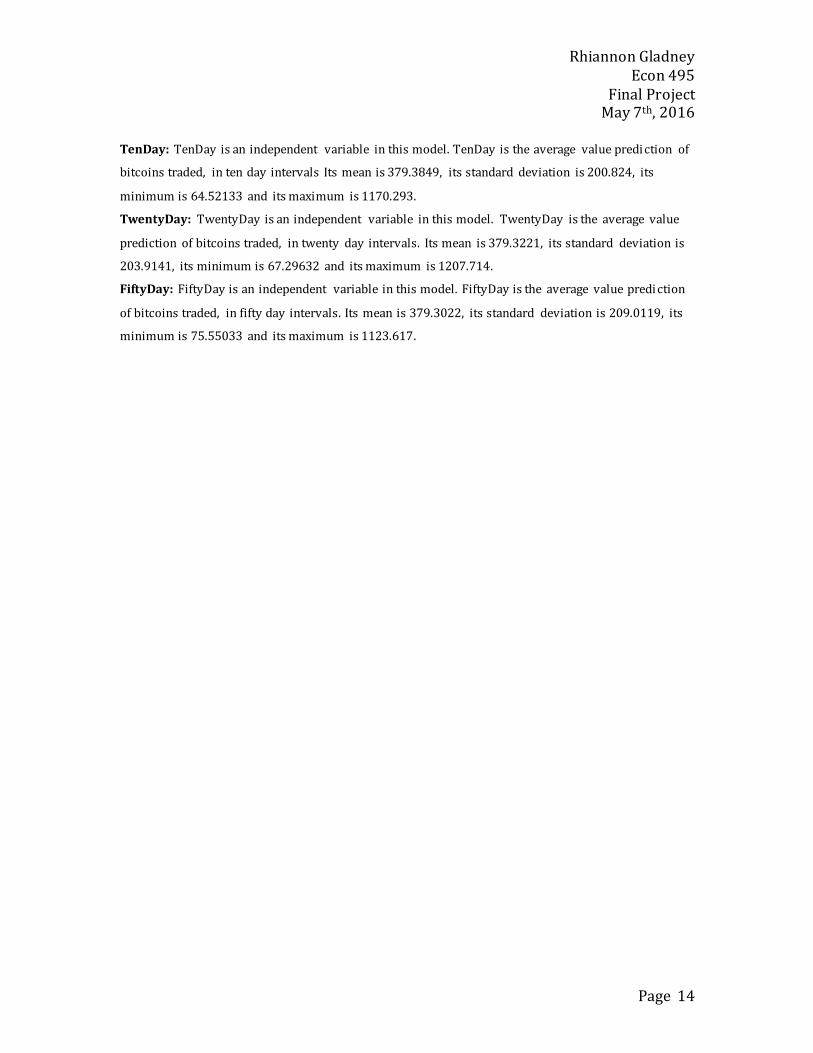
TenDay: TenDay is an independent variable in this model. TenDay is the average value prediction of
bitcoins traded, in ten day intervals Its mean is 379.3849, its standard deviation is 200.824, its
minimum is 64.52133 and its maximum is 1170.293.
TwentyDay: TwentyDay is an independent variable in this model. TwentyDay is the average value
prediction of bitcoins traded, in twenty day intervals. Its mean is 379.3221, its standard deviation is
203.9141, its minimum is 67.29632 and its maximum is 1207.714.
FiftyDay: FiftyDay is an independent variable in this model. FiftyDay is the average value prediction
of bitcoins traded, in fifty day intervals. Its mean is 379.3022, its standard deviation is 209.0119, its
minimum is 75.55033 and its maximum is 1123.617.

Rhiannon Gladney Econ 495
Final Project May 7th, 2016
Page 15
V. Empirical Results: Table 3: Regression Results of the Model
The partial regression coefficients represent small marginal contributions of individual
predictions of variation. There is not much change in variation over time, even when measuring with
different time intervals. TwoDay and FiftyDay are the variables that are most significant. The number
of observations used in this model could be higher in order to get more accurate results. The R-
squared is also alarmingly high. Issues aside, the results of this model conclude that prices have
remained relatively stable since 2014.
Variables: Price: Price is the dependent variable of this model. It represents the average value of bitcoins
traded for the day. Its coefficient is 4.115187, its standard error is 1.658349, its P-Value is 0.00, and
its sign is not applicable. This is a significant variable.
Same: Same is an independent variable in this model. It represents that prediction that the average
value of bitcoins will be the same as the day before. Its coefficient is 0.7820214, its standard error is
0.1161428, its P-Value is 0.572, and its sign is positive. This is not a significant variable.
TwoDay: TwoDay is an independent variable in this model. TwoDay is the average value prediction
of bitcoins traded, in two day intervals. Its coefficient is 0.0343532, its standard error is 0.0608178,
its P-Value is 0.015, and its sign is positive. This is a significant variable.

Rhiannon Gladney Econ 495
Final Project May 7th, 2016
Page 16
FiveDay: FiveDay is an independent variable in this model. FiveDay is the average value prediction of
bitcoins traded, in five day intervals. Its coefficient is -0.1807502, its standard error is 0.0740712, its
P-Value is 0.00, and its sign is negative. This is a significant variable.
SevenDay: SevenDay is an independent variable in this model. SevenDay is the average value
prediction of bitcoins traded, in seven day intervals. Its coefficient is 0.4413013, its standard error is
0.0785681, its P-Value is 0.012 and its sign is positive. This is a significant variable.
TenDay: TenDay is an independent variable in this model. TenDay is the average value prediction of
bitcoins traded, in ten day intervals. Its coefficient is -0.1634128, its standard error is 0.0646604, its
P-Value is 0.022, and its sign is negative. This is a significant variable.
TwentyDay: TwentyDay is an independent variable in this model. TwentyDay is the average value
prediction of bitcoins traded, in twenty day intervals. Its coefficient is 0.0766486, its standard error
is 0.0333536, its P-Value is 0.987, and its sign is positive. This is not a significant variable.
FiftyDay: FiftyDay is an independent variable in this model. FiftyDay is the average value prediction
of bitcoins traded, in fifty day intervals. Its coefficient is -0.0002836, its standard error is 0.0169855,
its P-Value is -0.013, and its sign is negative. This is a significant variable.
Table 4: Regression Results of the Model (in Log Form)
The log transformations of variables can be used to make skewed distributions less skewed.
This is valuable because it makes patterns in the data more interpretable and it helps to meet the
assumptions of inferential statistics. In this case, the distributions did become less skewed. Most
notably: Same is not significant, however, LSame is significant. FiveDay is significant, however,
LFiveDay is not significant. Both TwentyDay and LTwentyDay are not significant.

Rhiannon Gladney Econ 495
Final Project May 7th, 2016
Page 17
Variables (in Log Form): LPrice: Price is the dependent variable of this model. It represents the average value of bitcoins
traded for the day. Its log coefficient is 0.0241, its standard error is 0.0136, its P-Value is 0.078, and
its sign is not applicable. This is a significant variable.
LSame: Log of Same is an independent variable in this model. It represents that prediction that the
average value of bitcoins will be the same as the day before. Its coefficient is 1.39, its standard error
is 0.19, its P-Value is 0.00, and its sign is positive. This is a significant variable.
LTwoDay: Log of TwoDay is an independent variable in this model. TwoDay is the average value
prediction of bitcoins traded, in two day intervals. Its coefficient is -0.96, its standard error is 0.052,
its P-Value is 0.065, and its sign is negative. This is a significant variable.
LFiveDay: Log of FiveDay is an independent variable in this model. FiveDay is the average value
prediction of bitcoins traded, in five day intervals. Its coefficient is -0.02633, its standard error is
0.1129, its P-Value is 0.818, and its sign is negative. This is a not significant variable.
LSevenDay: Log of SevenDay is an independent variable in this model. SevenDay is the average value
prediction of bitcoins traded, in seven day intervals. Its coefficient is 0.1967, its standard error is
0.0855, its P-Value is 0.684 and its sign is positive. This is a significant variable.
LTenDay: Log of TenDay is an independent variable in this model. TenDay is the average value
prediction of bitcoins traded, in ten day intervals. Its coefficient is -0.1845, its standard error is
0.0618, its P-Value is 0.003, and its sign is negative. This is a significant variable.
LTwentyDay: Log of TwentyDay is an independent variable in this model. TwentyDay is the average
value prediction of bitcoins traded, in twenty day intervals. Its coefficient is -0.0317, its standard
error is 0.0337, its P-Value is 0.684, and its sign is negative. This is not a significant variable.
LFiftyDay: Log of FiftyDay is an independent variable in this model. FiftyDay is the average value
prediction of bitcoins traded, in fifty day intervals. Its coefficient is -0.0547, its standard error is
0.0201, its P-Value is -0.007, and its sign is negative. This is a significant variable.

Rhiannon Gladney Econ 495
Final Project May 7th, 2016
Page 18
Figure 1: Bitcoin Price Volatility Time Series
‘
This is a price volatility time series line graph. It visually displays how bitcoin’s prices in the
beginning, in 2009, were very unstable. In 2014, bitcoin’s price began to stabilize,
Figure 2: Bitcoin to US Dollar Exchange Rate in May 2016

Rhiannon Gladney Econ 495
Final Project May 7th, 2016
Page 19
The Bitcoin to US Dollar exchange rate was 1 Bitcoin roughly $458.50 US Dollars in May of
2016; this represents the price value of a Bitcoin as of May 2nd 2016. Until June of 2016, Bitcoin has
been in the $400 to $1 US dollar range until since 2014.
Figure 3: Bitcoin to US Dollar Exchange Rate in June 2016 (Includes Brexit Break)
In June of 2016, Bitcoin experienced its first major spike in two years due to speculation
regarding Brexit, the United Kingdom leaving the European Union. Considering, all of the major
currencies had major shifts de to Brexit, it is still fair to say that bitcoin’s price is stable.
Figure 4: US Dollar to Euro Exchange Rate in June 2016 (Includes Brexit Break)

Rhiannon Gladney Econ 495
Final Project May 7th, 2016
Page 20
Figure 5: Euro to US Dollar Exchange Rate in June 2016 (Includes Brexit Break)
Figure 6: British Pound to US Dollar Exchange Rate in June 2016 (Includes Brexit Break)
Upon first glance, the bitcoin price fluctuation graph looks more unstable than the US, Dollar,
the Euro, and the British Pound price fluctuation graphs. However, volume needs to be accounted for.
There are simply a lot more US dollars out there than there are bitcoins. Even at the peak of the most
recent bubble, the total value of bitcoins was less than $3 billion. Whereas the US dollar supply is
nearly $10 trillion. Considering bitcoin’s low volume, it has proved to be as stable as any of the other
major currencies. It is not wild to say that bitcoin has the possibility of becoming even more stable
than the US dollar, the global currency. If this becomes the case, it is safe to say that there will be an
increase in demand for bitcoin investments.

Rhiannon Gladney Econ 495
Final Project May 7th, 2016
Page 21
Unit Root Tests: Augmented Dickey Fuller & Phillips-Perron
Cointegration has become a valuable property in modern time series analysis. Time series
often have trends; trends that are either deterministic or stochastic. To account for this, unit root
tests must be performed. In this report, the Dickey-Fuller Test and the Phillips-Perron Test will be
used.
Table 5: Augmented Dickey-Fuller Results:

Rhiannon Gladney Econ 495
Final Project May 7th, 2016
Page 22
*These results are in levels
The Dickey-Fuller test tests if the null hypothesis of a unit root can be rejected. In other
words, it tests to see if the model is stationary. In this case, the variables prove to be stationary. The
residuals are negative and relatively close to zero.

Rhiannon Gladney Econ 495
Final Project May 7th, 2016
Page 23
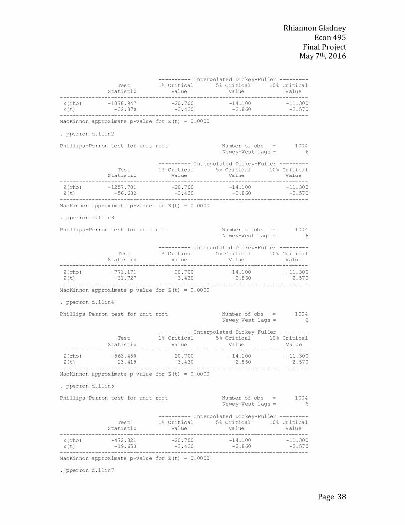
Table 6: Phillips-Perron Results:

Rhiannon Gladney Econ 495
Final Project May 7th, 2016
Page 24
The Phillips-Perron test is used in time series analysis to test if the null hypothesis is
integrated of order 1. It adds to the Dickey-Fuller test by testing if the process for generating the data
might have had a higher order of autocorrelation. To account for autocorrelation, the Phillips-Perron
test makes a non-parametric correction to the test statistic. In this case, there were very minimal
adjustments.

Rhiannon Gladney Econ 495
Final Project May 7th, 2016
Page 25
VI. Conclusion: Bitcoin is both a digital asset and a payment system. In 2008, bitcoins were first published
and developed by the allusive Satoshi Nakamoto. This new system does not require a financial
intermediary; in other words, it is peer-to- peer. The transactions are verified by network nodes and
then recorded in a ledger, the blockchain. The blockchain uses bitcoins as its unit of account. This
system does require a central repository or an administrator. With that being said, bitcoin is the very
first decentralized digital currency and is considered the first successful cryptocurrency.
Putting bank opposition, price fluctuations, and bitcoin’s ‘bad’ reputation aside, Bitcoin is
just a currency; it is a currency with great potential. Paired with the blockchain system, bitcoins have
to the potential to create a new way to buy and purchase items securely and affordably. This report
attempted to answer the question: Do bitcoin and the Blockchain, together, provide a secure and
affordable system for financial transactions that is not being widely implemented because of bitcoin’s
‘fluctuating prices’, and because of bitcoin’s infamous reputation? Mainly, this report focused on
bitcoin’s fluctuating prices because they are much more testable than bitcoin’s reputation.
Putting the potential issues with the model used aside, the descriptive statistics and
empirical results of the model conclude that bitcoin’s prices have stabilized since 2014.

Rhiannon Gladney Econ 495
Final Project May 7th, 2016
Page 26
VII. References
• Andrychowicz, M. "Secure Multiparty Computations on Bitcoin." University of
Warsaw, May 2014. Web. Apr. 2016.
• Bojanova, Irena. "Bitcoin: Benefit or Curse?" IEEE Xplore. IEEE Computer
Society, May-June 2014. Web. Apr. 2016.
• Bonneau, J. "Research Perspectives and Challenges for Bitcoin
Cryptocurrencies." N.p., May 2015. Web. Apr. 2016.
• Bradbury, Danny. "The Problem with Bitcoin." N.p., n.d. Web. Apr. 2016.
• CARL, L. Blockchain.info. Retrieved April 13, 2016.
• Eyal, Ittay. "Majority Is Not Enough: Bitcoin Mining Is Vulnerable." N.p., Nov.
2013. Web. Apr. 2016.
• Hurlburt, George. "Might the Blockchain Outlive Bitcoin?" IEEE Xplore. IEEE
Computer Society, Mar.-Apr. 2016. Web. Apr. 2016.
• Kraft, D. Difficulty control for blockchain-based consensus systems. April 15,
2015.Retrieved April 13, 2016.
• Melin, Mark. "Nasdaq Adopts Bitcoin Blockchain Technology." Newstex
Global Business, May 2015. Web. Apr. 2016.
• Möser, M. "An Inquiry into Money Laundering Tools in the Bitcoin
Ecosystem." Univ. of Munster, n.d. Web. Apr. 2016.
• Newstex. "Banks Using the Bitcoin Blockchain Is like Putting a Bird in a
Cage." Newstex Finance and Accounting, Oct. 2014. Web. Apr. 2016.
• Singh, P. Performance Comparison of Executing Fast Transactions in Bitcoin
Network Using Verifiable Code Execution. 2013. Retrieved April 13, 2016

Rhiannon Gladney Econ 495
Final Project May 7th, 2016
Page 27
VIII. Appendix
delta: 1 day
time variable: date, 4/22/2013 to 3/3/2016, but with gaps
. tsset date, daily
lin50 1,032 379.3022 209.0119 75.55033 1123.617
lin20 1,032 379.3221 203.9141 67.29632 1207.714
lin10 1,032 379.3849 200.824 64.52133 1170.293
lin7 1,032 379.4032 200.055 63.07714 1200.221
lin5 1,032 379.4185 199.8558 62.703 1213.178
lin2 1,032 379.4512 201.0037 63.74 1191.69
same 1,032 379.1147 198.1887 69.05 1132.26
actual 1,032 379.4471 198.0156 69.05 1132.26
Variable Obs Mean Std. Dev. Min Max
. sum actual same lin2 lin5 lin7 lin10 lin20 lin50
_cons 4.115187 1.658349 2.48 0.013 .8610355 7.369338
lin50 -.0002863 .0169855 -0.02 0.987 -.0336167 .0330441
lin20 .0766486 .0333536 2.30 0.022 .0111993 .1420979
lin10 -.1634128 .0646604 -2.53 0.012 -.2902948 -.0365308
lin7 .4413013 .0785681 5.62 0.000 .2871284 .5954741
lin5 -.1807502 .0740712 -2.44 0.015 -.3260989 -.0354015
lin2 .0343532 .0608178 0.56 0.572 -.0849886 .153695
same .7820214 .1661428 4.71 0.000 .4560021 1.108041
actual Coef. Std. Err. t P>|t| [95% Conf. Interval]
Total 40425682.7 1,031 39210.1675 Root MSE = 23.987
Adj R-squared = 0.9853
Residual 589193.579 1,024 575.384354 R-squared = 0.9854
Model 39836489.1 7 5690927.01 Prob > F = 0.0000
F(7, 1024) = 9890.65
Source SS df MS Number of obs = 1,032
. regress actual same lin2 lin5 lin7 lin10 lin20 lin50
lin50 0.9431 1.0000
actual 1.0000
actual lin50
(obs=1,032)
. corr actual lin50
same 0.9924 1.0000
actual 1.0000
actual same
(obs=1,032)
. corr actual same

Rhiannon Gladney Econ 495
Final Project May 7th, 2016
Page 28
55. 6/15/2013 100.79 100.24
54. 6/14/2013 100.24 101.33
53. 6/13/2013 101.33 101.46
52. 6/12/2013 101.46 104.48
51. 6/11/2013 104.48 100.15
50. 6/10/2013 100.15 97.5
49. 6/9/2013 97.5 96.84
48. 6/8/2013 96.84 92.72
47. 6/7/2013 92.72 93.13
46. 6/6/2013 93.13 93.4
45. 6/5/2013 93.4 91.07
44. 6/4/2013 91.07 90.9
43. 6/3/2013 90.9 88.33
42. 6/2/2013 88.33 87.78
41. 6/1/2013 87.78 89.09
40. 5/31/2013 89.09 89.65
39. 5/30/2013 89.65 88.31
38. 5/29/2013 88.31 95.32
37. 5/28/2013 95.32 95.2
36. 5/27/2013 95.2 96.51
35. 5/26/2013 96.51 93.97
34. 5/25/2013 93.97 91.8
33. 5/24/2013 91.8 95.07
32. 5/23/2013 95.07 86.41
31. 5/22/2013 86.41 81.09
30. 5/21/2013 81.09 74.49
29. 5/20/2013 74.49 76
28. 5/19/2013 76 70.26
27. 5/18/2013 70.26 69.05
26. 5/17/2013 69.05 70.82
25. 5/16/2013 70.82 77.9
24. 5/15/2013 77.9 82.75
23. 5/14/2013 82.75 88.13
22. 5/13/2013 88.13 89.03
21. 5/12/2013 89.03 94.26
20. 5/11/2013 94.26 95.08
19. 5/10/2013 95.08 95.06
18. 5/9/2013 95.06 100.59
17. 5/8/2013 100.59 102.27
16. 5/7/2013 102.27 103.65
15. 5/6/2013 103.65 101.35
14. 5/5/2013 101.35 104.93
13. 5/4/2013 104.93 105.02
12. 5/3/2013 105.02 108.13
11. 5/2/2013 108.13 110.04
10. 5/1/2013 110.04 106.95
9. 4/30/2013 106.95 106.87
8. 4/29/2013 106.87 100.72
7. 4/28/2013 100.72 99.92
6. 4/27/2013 99.92 100.38
5. 4/26/2013 100.38 100.54
4. 4/25/2013 100.54 105.08
3. 4/24/2013 105.08 108.85
2. 4/23/2013 108.85 106.83
1. 4/22/2013 106.83 104.68
date actual same
. list date actual same

Rhiannon Gladney Econ 495
Final Project May 7th, 2016
Page 29
name: <unnamed>
log: d:\bitcoin.log
log type: text
opened on: 17 Jul 2016, 09:39:58
. insheet using d:\bitcoin.txt
(11 vars, 1032 obs)
. save d:\bitcoin, replace
file d:\bitcoin.dta saved
.
. gen daily=date(day, "MDY")
. sum actual same lin2 lin3 lin4 lin5 lin7 lin10 lin20 lin50
Variable | Obs Mean Std. Dev. Min Max
-------------+--------------------------------------------------------
actual | 1032 379.4471 198.0156 69.05 1132.26
same | 1032 379.1147 198.1887 69.05 1132.26
lin2 | 1032 379.4512 201.0037 63.74 1191.69
lin3 | 1032 379.44 200.1871 63.74 1214.95
lin4 | 1032 379.4295 199.9485 63.085 1211.7
-------------+--------------------------------------------------------
lin5 | 1032 379.4185 199.8558 62.703 1213.178
lin7 | 1032 379.4032 200.055 63.07714 1200.221
lin10 | 1032 379.3849 200.824 64.52133 1170.293
lin20 | 1032 379.3221 203.9141 67.29632 1207.714
lin50 | 1032 379.3022 209.0119 75.55033 1123.617
.
. gen lactual=ln(actual)
. gen lsame=ln(same)
. gen llin2=ln(lin2)
. gen llin3=ln(lin3)
. gen llin4=ln(lin4)
. gen llin5=ln(lin5)
. gen llin7=ln(lin7)
. gen llin10=ln(lin10)
. gen llin20=ln(lin20)
. gen llin50=ln(lin50)
.
. tsset daily
time variable: daily, 19470 to 20516, but with gaps
delta: 1 unit
. ** Here I am ussing the Augmented Dickey-Fuller unit root test; the variable
. ** are in levels
. dfuller lactual
Dickey-Fuller test for unit root Number of obs = 1017
---------- Interpolated Dickey-Fuller ---------
Test 1% Critical 5% Critical 10% Critical

Rhiannon Gladney Econ 495
Final Project May 7th, 2016
Page 30
Statistic Value Value Value
------------------------------------------------------------------------------
Z(t) -1.690 -3.430 -2.860 -2.570
------------------------------------------------------------------------------
MacKinnon approximate p-value for Z(t) = 0.4363
. dfuller lsame
Dickey-Fuller test for unit root Number of obs = 1017
---------- Interpolated Dickey-Fuller ---------
Test 1% Critical 5% Critical 10% Critical
Statistic Value Value Value
------------------------------------------------------------------------------
Z(t) -1.800 -3.430 -2.860 -2.570
------------------------------------------------------------------------------
MacKinnon approximate p-value for Z(t) = 0.3806
. dfuller llin2
Dickey-Fuller test for unit root Number of obs = 1017
---------- Interpolated Dickey-Fuller ---------
Test 1% Critical 5% Critical 10% Critical
Statistic Value Value Value
------------------------------------------------------------------------------
Z(t) -3.084 -3.430 -2.860 -2.570
------------------------------------------------------------------------------
MacKinnon approximate p-value for Z(t) = 0.0277
. dfuller llin3
Dickey-Fuller test for unit root Number of obs = 1017
---------- Interpolated Dickey-Fuller ---------
Test 1% Critical 5% Critical 10% Critical
Statistic Value Value Value
------------------------------------------------------------------------------
Z(t) -2.331 -3.430 -2.860 -2.570
------------------------------------------------------------------------------
MacKinnon approximate p-value for Z(t) = 0.1621
. dfuller llin4
Dickey-Fuller test for unit root Number of obs = 1017
---------- Interpolated Dickey-Fuller ---------
Test 1% Critical 5% Critical 10% Critical
Statistic Value Value Value
------------------------------------------------------------------------------
Z(t) -2.120 -3.430 -2.860 -2.570
------------------------------------------------------------------------------
MacKinnon approximate p-value for Z(t) = 0.2367
. dfuller llin5
Dickey-Fuller test for unit root Number of obs = 1017
---------- Interpolated Dickey-Fuller ---------
Test 1% Critical 5% Critical 10% Critical
Statistic Value Value Value
------------------------------------------------------------------------------
Z(t) -1.989 -3.430 -2.860 -2.570
------------------------------------------------------------------------------
MacKinnon approximate p-value for Z(t) = 0.2915

Rhiannon Gladney Econ 495
Final Project May 7th, 2016
Page 31
. dfuller llin7
Dickey-Fuller test for unit root Number of obs = 1017
---------- Interpolated Dickey-Fuller ---------
Test 1% Critical 5% Critical 10% Critical
Statistic Value Value Value
------------------------------------------------------------------------------
Z(t) -1.931 -3.430 -2.860 -2.570
------------------------------------------------------------------------------
MacKinnon approximate p-value for Z(t) = 0.3177
. dfuller llin10
Dickey-Fuller test for unit root Number of obs = 1017
---------- Interpolated Dickey-Fuller ---------
Test 1% Critical 5% Critical 10% Critical
Statistic Value Value Value
------------------------------------------------------------------------------
Z(t) -1.808 -3.430 -2.860 -2.570
------------------------------------------------------------------------------
MacKinnon approximate p-value for Z(t) = 0.3765
. dfuller llin20
Dickey-Fuller test for unit root Number of obs = 1017
---------- Interpolated Dickey-Fuller ---------
Test 1% Critical 5% Critical 10% Critical
Statistic Value Value Value
------------------------------------------------------------------------------
Z(t) -1.887 -3.430 -2.860 -2.570
------------------------------------------------------------------------------
MacKinnon approximate p-value for Z(t) = 0.3382
. dfuller llin50
Dickey-Fuller test for unit root Number of obs = 1017
---------- Interpolated Dickey-Fuller ---------
Test 1% Critical 5% Critical 10% Critical
Statistic Value Value Value
------------------------------------------------------------------------------
Z(t) -2.119 -3.430 -2.860 -2.570
------------------------------------------------------------------------------
MacKinnon approximate p-value for Z(t) = 0.2369
.
. ** Here I am ussing the Augmented Dickey-Fuller unit root test; the variable
. ** are in first difference form
.
. dfuller d.lactual
Dickey-Fuller test for unit root Number of obs = 1004
---------- Interpolated Dickey-Fuller ---------
Test 1% Critical 5% Critical 10% Critical
Statistic Value Value Value
------------------------------------------------------------------------------
Z(t) -30.739 -3.430 -2.860 -2.570
------------------------------------------------------------------------------
MacKinnon approximate p-value for Z(t) = 0.0000
. dfuller d.lsame
Dickey-Fuller test for unit root Number of obs = 1004

Rhiannon Gladney Econ 495
Final Project May 7th, 2016
Page 32
---------- Interpolated Dickey-Fuller ---------
Test 1% Critical 5% Critical 10% Critical
Statistic Value Value Value
------------------------------------------------------------------------------
Z(t) -32.944 -3.430 -2.860 -2.570
------------------------------------------------------------------------------
MacKinnon approximate p-value for Z(t) = 0.0000

Rhiannon Gladney Econ 495
Final Project May 7th, 2016
Page 33
. dfuller d.llin2
Dickey-Fuller test for unit root Number of obs = 1004
---------- Interpolated Dickey-Fuller ---------
Test 1% Critical 5% Critical 10% Critical
Statistic Value Value Value
------------------------------------------------------------------------------
Z(t) -49.819 -3.430 -2.860 -2.570
------------------------------------------------------------------------------
MacKinnon approximate p-value for Z(t) = 0.0000
. dfuller d.llin3
Dickey-Fuller test for unit root Number of obs = 1004
---------- Interpolated Dickey-Fuller ---------
Test 1% Critical 5% Critical 10% Critical
Statistic Value Value Value
------------------------------------------------------------------------------
Z(t) -30.847 -3.430 -2.860 -2.570
------------------------------------------------------------------------------
MacKinnon approximate p-value for Z(t) = 0.0000
. dfuller d.llin4
Dickey-Fuller test for unit root Number of obs = 1004
---------- Interpolated Dickey-Fuller ---------
Test 1% Critical 5% Critical 10% Critical
Statistic Value Value Value
------------------------------------------------------------------------------
Z(t) -23.967 -3.430 -2.860 -2.570
------------------------------------------------------------------------------
MacKinnon approximate p-value for Z(t) = 0.0000
. dfuller d.llin5
Dickey-Fuller test for unit root Number of obs = 1004
---------- Interpolated Dickey-Fuller ---------
Test 1% Critical 5% Critical 10% Critical
Statistic Value Value Value
------------------------------------------------------------------------------
Z(t) -20.377 -3.430 -2.860 -2.570
------------------------------------------------------------------------------
MacKinnon approximate p-value for Z(t) = 0.0000
. dfuller d.llin7
Dickey-Fuller test for unit root Number of obs = 1004
---------- Interpolated Dickey-Fuller ---------
Test 1% Critical 5% Critical 10% Critical
Statistic Value Value Value
------------------------------------------------------------------------------
Z(t) -16.368 -3.430 -2.860 -2.570
------------------------------------------------------------------------------
MacKinnon approximate p-value for Z(t) = 0.0000

Rhiannon Gladney Econ 495
Final Project May 7th, 2016
Page 34
. dfuller d.llin10
Dickey-Fuller test for unit root Number of obs = 1004
---------- Interpolated Dickey-Fuller ---------
Test 1% Critical 5% Critical 10% Critical
Statistic Value Value Value
------------------------------------------------------------------------------
Z(t) -13.541 -3.430 -2.860 -2.570
------------------------------------------------------------------------------
MacKinnon approximate p-value for Z(t) = 0.0000
. dfuller d.llin20
Dickey-Fuller test for unit root Number of obs = 1004
---------- Interpolated Dickey-Fuller ---------
Test 1% Critical 5% Critical 10% Critical
Statistic Value Value Value
------------------------------------------------------------------------------
Z(t) -9.092 -3.430 -2.860 -2.570
------------------------------------------------------------------------------
MacKinnon approximate p-value for Z(t) = 0.0000
. dfuller d.llin50
Dickey-Fuller test for unit root Number of obs = 1004
---------- Interpolated Dickey-Fuller ---------
Test 1% Critical 5% Critical 10% Critical
Statistic Value Value Value
------------------------------------------------------------------------------
Z(t) -5.100 -3.430 -2.860 -2.570
------------------------------------------------------------------------------
MacKinnon approximate p-value for Z(t) = 0.0000
.
. ** Here I am ussing the Phillips-Perron unit root test; the variable
. ** are in levels
. pperron lactual
Phillips-Perron test for unit root Number of obs = 1017
Newey-West lags = 6
---------- Interpolated Dickey-Fuller ---------
Test 1% Critical 5% Critical 10% Critical
Statistic Value Value Value
------------------------------------------------------------------------------
Z(rho) -4.292 -20.700 -14.100 -11.300
Z(t) -1.734 -3.430 -2.860 -2.570
------------------------------------------------------------------------------
MacKinnon approximate p-value for Z(t) = 0.4138
. pperron lsame
Phillips-Perron test for unit root Number of obs = 1017
Newey-West lags = 6
---------- Interpolated Dickey-Fuller ---------
Test 1% Critical 5% Critical 10% Critical
Statistic Value Value Value
------------------------------------------------------------------------------
Z(rho) -4.501 -20.700 -14.100 -11.300
Z(t) -1.824 -3.430 -2.860 -2.570
------------------------------------------------------------------------------
MacKinnon approximate p-value for Z(t) = 0.3684

Rhiannon Gladney Econ 495
Final Project May 7th, 2016
Page 35

Rhiannon Gladney Econ 495
Final Project May 7th, 2016
Page 36
. pperron llin2
Phillips-Perron test for unit root Number of obs = 1017
Newey-West lags = 6
---------- Interpolated Dickey-Fuller ---------
Test 1% Critical 5% Critical 10% Critical
Statistic Value Value Value
------------------------------------------------------------------------------
Z(rho) -6.891 -20.700 -14.100 -11.300
Z(t) -1.994 -3.430 -2.860 -2.570
------------------------------------------------------------------------------
MacKinnon approximate p-value for Z(t) = 0.2894
. pperron llin3
Phillips-Perron test for unit root Number of obs = 1017
Newey-West lags = 6
---------- Interpolated Dickey-Fuller ---------
Test 1% Critical 5% Critical 10% Critical
Statistic Value Value Value
------------------------------------------------------------------------------
Z(rho) -6.210 -20.700 -14.100 -11.300
Z(t) -2.064 -3.430 -2.860 -2.570
------------------------------------------------------------------------------
MacKinnon approximate p-value for Z(t) = 0.2592
. pperron llin4
Phillips-Perron test for unit root Number of obs = 1017
Newey-West lags = 6
---------- Interpolated Dickey-Fuller ---------
Test 1% Critical 5% Critical 10% Critical
Statistic Value Value Value
------------------------------------------------------------------------------
Z(rho) -6.177 -20.700 -14.100 -11.300
Z(t) -2.112 -3.430 -2.860 -2.570
------------------------------------------------------------------------------
MacKinnon approximate p-value for Z(t) = 0.2399
. pperron llin5
Phillips-Perron test for unit root Number of obs = 1017
Newey-West lags = 6
---------- Interpolated Dickey-Fuller ---------
Test 1% Critical 5% Critical 10% Critical
Statistic Value Value Value
------------------------------------------------------------------------------
Z(rho) -6.039 -20.700 -14.100 -11.300
Z(t) -2.094 -3.430 -2.860 -2.570
------------------------------------------------------------------------------
MacKinnon approximate p-value for Z(t) = 0.2471
. pperron llin7
Phillips-Perron test for unit root Number of obs = 1017
Newey-West lags = 6
---------- Interpolated Dickey-Fuller ---------
Test 1% Critical 5% Critical 10% Critical
Statistic Value Value Value
------------------------------------------------------------------------------
Z(rho) -6.103 -20.700 -14.100 -11.300

Rhiannon Gladney Econ 495
Final Project May 7th, 2016
Page 37
Z(t) -2.096 -3.430 -2.860 -2.570
------------------------------------------------------------------------------
MacKinnon approximate p-value for Z(t) = 0.2463
. pperron llin10
Phillips-Perron test for unit root Number of obs = 1017
Newey-West lags = 6
---------- Interpolated Dickey-Fuller ---------
Test 1% Critical 5% Critical 10% Critical
Statistic Value Value Value
------------------------------------------------------------------------------
Z(rho) -5.893 -20.700 -14.100 -11.300
Z(t) -2.014 -3.430 -2.860 -2.570
------------------------------------------------------------------------------
MacKinnon approximate p-value for Z(t) = 0.2805
. pperron llin20
Phillips-Perron test for unit root Number of obs = 1017
Newey-West lags = 6
---------- Interpolated Dickey-Fuller ---------
Test 1% Critical 5% Critical 10% Critical
Statistic Value Value Value
------------------------------------------------------------------------------
Z(rho) -4.765 -20.700 -14.100 -11.300
Z(t) -1.862 -3.430 -2.860 -2.570
------------------------------------------------------------------------------
MacKinnon approximate p-value for Z(t) = 0.3502
. pperron llin50
Phillips-Perron test for unit root Number of obs = 1017
Newey-West lags = 6
---------- Interpolated Dickey-Fuller ---------
Test 1% Critical 5% Critical 10% Critical
Statistic Value Value Value
------------------------------------------------------------------------------
Z(rho) -3.147 -20.700 -14.100 -11.300
Z(t) -1.648 -3.430 -2.860 -2.570
------------------------------------------------------------------------------
MacKinnon approximate p-value for Z(t) = 0.4582
.
. ** Here I am ussing the Phillips-Perron unit root test; the variable
. ** are in difference form
. pperron d.lactual
Phillips-Perron test for unit root Number of obs = 1004
Newey-West lags = 6
---------- Interpolated Dickey-Fuller ---------
Test 1% Critical 5% Critical 10% Critical
Statistic Value Value Value
------------------------------------------------------------------------------
Z(rho) -1014.997 -20.700 -14.100 -11.300
Z(t) -30.800 -3.430 -2.860 -2.570
------------------------------------------------------------------------------
MacKinnon approximate p-value for Z(t) = 0.0000
. pperron d.lsame
Phillips-Perron test for unit root Number of obs = 1004
Newey-West lags = 6
Rhiannon Gladney Econ 495
Final Project May 7th, 2016
Page 38
---------- Interpolated Dickey-Fuller ---------
Test 1% Critical 5% Critical 10% Critical
Statistic Value Value Value
------------------------------------------------------------------------------
Z(rho) -1078.947 -20.700 -14.100 -11.300
Z(t) -32.870 -3.430 -2.860 -2.570
------------------------------------------------------------------------------
MacKinnon approximate p-value for Z(t) = 0.0000
. pperron d.llin2
Phillips-Perron test for unit root Number of obs = 1004
Newey-West lags = 6
---------- Interpolated Dickey-Fuller ---------
Test 1% Critical 5% Critical 10% Critical
Statistic Value Value Value
------------------------------------------------------------------------------
Z(rho) -1257.701 -20.700 -14.100 -11.300
Z(t) -56.682 -3.430 -2.860 -2.570
------------------------------------------------------------------------------
MacKinnon approximate p-value for Z(t) = 0.0000
. pperron d.llin3
Phillips-Perron test for unit root Number of obs = 1004
Newey-West lags = 6
---------- Interpolated Dickey-Fuller ---------
Test 1% Critical 5% Critical 10% Critical
Statistic Value Value Value
------------------------------------------------------------------------------
Z(rho) -771.171 -20.700 -14.100 -11.300
Z(t) -31.727 -3.430 -2.860 -2.570
------------------------------------------------------------------------------
MacKinnon approximate p-value for Z(t) = 0.0000
. pperron d.llin4
Phillips-Perron test for unit root Number of obs = 1004
Newey-West lags = 6
---------- Interpolated Dickey-Fuller ---------
Test 1% Critical 5% Critical 10% Critical
Statistic Value Value Value
------------------------------------------------------------------------------
Z(rho) -563.450 -20.700 -14.100 -11.300
Z(t) -23.419 -3.430 -2.860 -2.570
------------------------------------------------------------------------------
MacKinnon approximate p-value for Z(t) = 0.0000
. pperron d.llin5
Phillips-Perron test for unit root Number of obs = 1004
Newey-West lags = 6
---------- Interpolated Dickey-Fuller ---------
Test 1% Critical 5% Critical 10% Critical
Statistic Value Value Value
------------------------------------------------------------------------------
Z(rho) -472.821 -20.700 -14.100 -11.300
Z(t) -19.653 -3.430 -2.860 -2.570
------------------------------------------------------------------------------
MacKinnon approximate p-value for Z(t) = 0.0000
. pperron d.llin7

Rhiannon Gladney Econ 495
Final Project May 7th, 2016
Page 39
Phillips-Perron test for unit root Number of obs = 1004
Newey-West lags = 6
---------- Interpolated Dickey-Fuller ---------
Test 1% Critical 5% Critical 10% Critical
Statistic Value Value Value
------------------------------------------------------------------------------
Z(rho) -369.324 -20.700 -14.100 -11.300
Z(t) -16.074 -3.430 -2.860 -2.570
------------------------------------------------------------------------------
MacKinnon approximate p-value for Z(t) = 0.0000
. pperron d.llin10
Phillips-Perron test for unit root Number of obs = 1004
Newey-West lags = 6
---------- Interpolated Dickey-Fuller ---------
Test 1% Critical 5% Critical 10% Critical
Statistic Value Value Value
------------------------------------------------------------------------------
Z(rho) -312.008 -20.700 -14.100 -11.300
Z(t) -14.189 -3.430 -2.860 -2.570
------------------------------------------------------------------------------
MacKinnon approximate p-value for Z(t) = 0.0000
. pperron d.llin20
Phillips-Perron test for unit root Number of obs = 1004
Newey-West lags = 6
---------- Interpolated Dickey-Fuller ---------
Test 1% Critical 5% Critical 10% Critical
Statistic Value Value Value
------------------------------------------------------------------------------
Z(rho) -154.082 -20.700 -14.100 -11.300
Z(t) -9.671 -3.430 -2.860 -2.570
------------------------------------------------------------------------------
MacKinnon approximate p-value for Z(t) = 0.0000
. pperron d.llin50
Phillips-Perron test for unit root Number of obs = 1004
Newey-West lags = 6
---------- Interpolated Dickey-Fuller ---------
Test 1% Critical 5% Critical 10% Critical
Statistic Value Value Value
------------------------------------------------------------------------------
Z(rho) -44.183 -20.700 -14.100 -11.300
Z(t) -5.089 -3.430 -2.860 -2.570
------------------------------------------------------------------------------
MacKinnon approximate p-value for Z(t) = 0.0000
.
. *** Here, I am estimating the log model
. reg lactual lsame llin2 llin3 llin4 llin5 llin7 llin10 llin20 llin50
Source | SS df MS Number of obs = 1032
-------------+------------------------------ F( 9, 1022) =20488.62
Model | 326.400119 9 36.2666798 Prob > F = 0.0000
Residual | 1.80903092 1022 .001770089 R-squared = 0.9945
-------------+------------------------------ Adj R-squared = 0.9944
Total | 328.209149 1031 .318340591 Root MSE = .04207
------------------------------------------------------------------------------

Rhiannon Gladney Econ 495
Final Project May 7th, 2016
Page 40
lactual | Coef. Std. Err. t P>|t| [95% Conf. Interval]
-------------+----------------------------------------------------------------
lsame | 1.398184 .1901512 7.35 0.000 1.025052 1.771315
llin2 | -.0960467 .0520253 -1.85 0.065 -.1981353 .0060419
llin3 | -.0416818 .0776889 -0.54 0.592 -.1941298 .1107661
llin4 | -.1820073 .1129358 -1.61 0.107 -.4036198 .0396051
llin5 | -.0263324 .1112416 -0.24 0.813 -.2446204 .1919556
llin7 | .1967558 .0855109 2.30 0.022 .0289589 .3645528
llin10 | -.1845026 .0618545 -2.98 0.003 -.305879 -.0631262
llin20 | -.0137035 .0337125 -0.41 0.684 -.0798571 .0524501
llin50 | -.0547127 .0201055 -2.72 0.007 -.0941654 -.0152599
_cons | .0241007 .0136436 1.77 0.078 -.0026719 .0508733
------------------------------------------------------------------------------

Rhiannon Gladney Econ 495
Final Project May 7th, 2016
Page 41
.
. *** The step below helps us testing for cointegration test using the Engel test
. predict e, resid
. dfuller e
Dickey-Fuller test for unit root Number of obs = 1017
---------- Interpolated Dickey-Fuller ---------
Test 1% Critical 5% Critical 10% Critical
Statistic Value Value Value
------------------------------------------------------------------------------
Z(t) -31.766 -3.430 -2.860 -2.570
------------------------------------------------------------------------------
MacKinnon approximate p-value for Z(t) = 0.0000
. pperron e
Phillips-Perron test for unit root Number of obs = 1017
Newey-West lags = 6
---------- Interpolated Dickey-Fuller ---------
Test 1% Critical 5% Critical 10% Critical
Statistic Value Value Value
------------------------------------------------------------------------------
Z(rho) -1054.850 -20.700 -14.100 -11.300
Z(t) -31.791 -3.430 -2.860 -2.570
------------------------------------------------------------------------------
MacKinnon approximate p-value for Z(t) = 0.0000
.
. ***Rhiannon mentioned a recent schock in Bitcoin value. We could test that
. *** by introducing Breaks in the analysis
.
. log close
name: <unnamed>
log: d:\bitcoin.log
log type: text
closed on: 17 Jul 2016, 09:39:58

Rhiannon Gladney Econ 495
Final Project May 7th, 2016
Page 42