undergraduate thesis major in mathematics faculty of...
TRANSCRIPT

Undergraduate Thesis
MAJOR IN MATHEMATICS
Faculty of Mathematics
University of Barcelona
NONCOOPERATIVE GAME THEORY: GENERALOVERVIEW AND ITS APPLICATION TO THE
STUDY OF COOPERATION
Adrià San José [email protected]
Advisor: Josep VivesBarcelona, January 29, 2015

Acknowledgements
I would like to express my deep gratitude to Professor Vives, my research supervisor, forhis guidance, encouragement and useful critiques of this undergraduate thesis. I wouldalso like to thank my friend Jaume Martí for suggesting I embarked on the study of GameTheory and also Alejandro de Miquel and Maddie Girard for patiently reading some ofthe parts of this project. Last but not least, I would like to thank my family - Montse,Antonio and Berta - for their support and encouragement throughout my study.
1

Contents
1 Introduction 41.1 Motivation: A First Example . . . . . . . . . . . . . . . . . . . . . . . . 4
1.1.1 Max-Min Strategy . . . . . . . . . . . . . . . . . . . . . . . . . . 61.1.2 Min-Max Strategy . . . . . . . . . . . . . . . . . . . . . . . . . . 71.1.3 Solution of the game . . . . . . . . . . . . . . . . . . . . . . . . . 8
2 Definition of Game and First Properties 102.1 What are games? . . . . . . . . . . . . . . . . . . . . . . . . . . . . . . . 102.2 Basic Concepts . . . . . . . . . . . . . . . . . . . . . . . . . . . . . . . . 112.3 Antagonistic Games . . . . . . . . . . . . . . . . . . . . . . . . . . . . . . 14
2.3.1 Equilibrium situations in antagonistic games . . . . . . . . . . . . 15
3 General Results Concerning Equilibrium Situations 163.1 Matrix Games . . . . . . . . . . . . . . . . . . . . . . . . . . . . . . . . . 163.2 Requirements for the existence of saddle points . . . . . . . . . . . . . . 16
3.2.1 Examples . . . . . . . . . . . . . . . . . . . . . . . . . . . . . . . 193.2.2 How should we play against an irrational player? . . . . . . . . . 19
4 Mixed Extensions of Matrix Games 214.1 Mixed Extension of a game . . . . . . . . . . . . . . . . . . . . . . . . . . 21
4.1.1 The MinMax Theorem . . . . . . . . . . . . . . . . . . . . . . . . 264.1.2 First Example . . . . . . . . . . . . . . . . . . . . . . . . . . . . . 274.1.3 Two lemmas . . . . . . . . . . . . . . . . . . . . . . . . . . . . . . 284.1.4 2×m games . . . . . . . . . . . . . . . . . . . . . . . . . . . . . 30
5 General Noncooperative Games 325.1 Mixed Extensions of Noncooperative Games . . . . . . . . . . . . . . . . 325.2 Nash’s Theorem . . . . . . . . . . . . . . . . . . . . . . . . . . . . . . . . 345.3 Examples . . . . . . . . . . . . . . . . . . . . . . . . . . . . . . . . . . . 36
5.3.1 The gender war . . . . . . . . . . . . . . . . . . . . . . . . . . . . 365.3.2 The swastika method . . . . . . . . . . . . . . . . . . . . . . . . . 365.3.3 Prisoner’s Dilemma - First approach . . . . . . . . . . . . . . . . 38
2

CONTENTS 3
6 A Mathematical Explanation of Cooperation 396.1 Prisoner’s Dilemma . . . . . . . . . . . . . . . . . . . . . . . . . . . . . . 406.2 Evolutionary Game Theory . . . . . . . . . . . . . . . . . . . . . . . . . 44
6.2.1 Basic Concepts . . . . . . . . . . . . . . . . . . . . . . . . . . . . 456.3 The Ultimatum Game . . . . . . . . . . . . . . . . . . . . . . . . . . . . 48
Conclusions 49
Bibliography 50

Chapter 1
Introduction
A game, in Game Theory, is a tool that can model any situation in which there arepeople that interact - taking decisions, making moves, etc - in order to attain a certaingoal. This mathematical description of conflicts began in the twentieth century thanksto the work of John Von Neumann, Oskar Morgenstern and John Nash and one of itsfirst motivations was to help military officers design optimal war strategies. Nowadays,however, Game Theory is applied to a wide range of disciplines, like Biology or PoliticalScience, but above all, to Economy. Interestingly, eleven game-theorists have won theEconomics Nobel Prize up to date but never has a Fields Medal been awarded to an expertin this field. This shows to what great extent Game Theory is important for Economyand at the same time how mathematicians regard it as a secondary discipline comparedto other areas of Mathematics. This undergraduate thesis clearly falls under the categoryof applied mathematics or mathematical modeling and therefore its goal is far from justaccurately proving a series of theorems. Instead, even if the foundations of Game Theorywill be laid, I will focus on showing how Game Theory can be applied to solve a greatnumber of different problems, like, for example, the emergence of cooperative dispositionstowards strangers.Bearing this in mind, I will begin this undergraduate thesis by analyzing a military conflictbetween two countries whose officials will have a symbolic name: Nash and Neumann.To so do, I warn the reader that I will informally explain and use certain results that willbe accurately justified later in this thesis. Let’s begin!
1.1 Motivation: A First Example
Suppose that a country A and a country B are at war and that the generals of each armyare called, respectively, John Nash and John Von Neumann. Every single day, Nash willsend a heavily armed bomber and a smaller support plane to attack B. To do so, hewill put a bomb in one of the two aircrafts. At the same time, Neumann knows Nash’sintentions and decides to embark on military action but judges unnecessary to attack thetwo planes, mainly for economic reasons. The bomber will survive 60% of the times it
4

CHAPTER 1. INTRODUCTION 5
suffers an attack and, if it manages to live through the raid, it will always hit the target.The lighter plane, which is not as precise, hits the target 70% of the times and plus onlysurvives Neumann’s attack half of the times. There are clearly only four possible results,which come from the combination of Nash choice to put the bomb either in the bomber orin the support plane, and Neumann’s call to attack one or the other aircraft. Nash feelsthat he gains when he hits the target and he does not care about suffering an attack onone of his planes. At the same time, Neumann desperately wants to protect his citizensand therefore he will lose utility when an attack is carried out. Nash’s gain for everypossible combination of strategies is:
Bomber attacked Support attackedBomb in bomber 0.6× 1 = 0.6 1
Bomb in support 0.7 0, 5× 0.7 = 0.35
Table 1.1. Nash’s Payoff
where we have assumed an increase in a unit of his utility comes from a successful attack.In an isolated realization of the game, the target can only either be or not be hit, so whatdo the numbers in the matrix represent? Clearly, the expected values of the outcome ofthe game when those strategies are employed. Given that this game is repeated everyday, the Law of Large Numbers guarantees that the average outcome of the confrontationof two strategies (let’s say for example "Bomb in bomber" against "Bomber attacked")will tend to its expected value (for the aforementioned strategies, 0.6). Therefore, thefollowing will be a good long-term analysis.Bear in mind that we should give the utility of both players, but here Neumann’s utilityhas implicitly been given as it will be the matrix on top with a minus sign in front of allentries.
Remark. text
1. Nash can make sure that at least 60% of the attacks are successful by always puttingthe bomb in the bomber, as we would only be dealing with the matrix’ first row.
2. Neumann can make sure that no more than 70% of the attacks are successful byattacking the bomber plane, as we would only be dealing with the matrix’ firstcolumn.
These facts could determine their strategies. If that was the case, the game would unfoldas a constant 0.6 gain for Nash. However, instead of always putting the bomb in thebomber, Nash decides, every now and then, to bluff and to put the bomb in the supportplane. How often should he do that? Which is the best percentage of success he can get?How should Neumann adapt to this change? Let’s give an answer to all this questions.Given that Nash will no longer stick to one of the strategies but combine them, he willstart to employ a so-called mixed strategy. Let’s use a probability distribution X = (a, b)

CHAPTER 1. INTRODUCTION 6
1 to encapsulate this, where it should be understood that Nash will put the bomb inthe bomber with a probability a and in the support plane with a probability b. Usingthis notation, a pure strategy is then (1, 0) -bomb always in the bomber- or (0, 1) -bombalways in the support plane. Let us denote by A the matrix of table 1.1. For any strategiesX ∈ S1 and Y ∈ S2 (Si should be understood as the set of all possible mixed strategiesof player i) we can calculate the expected payoff H(X, Y ) by ponderating the payoffs ofthe pure strategies, i.e., by calculating XAY T . For any strategy Nash (Neumann) picks,the strategy that minimizes the other’s payoff is called the optimal counterstrategy orthe best reply.
Theorem 1.1. If either Nash or Neumann employ a fixed strategy (and it means theywill not keep changing the probabilities of how they distribute their choices), then theopponent’s best reply is a pure strategy.
Proof. Assume Nash’s strategy is X = (1 − x, x) and Neumann’s Y = (1 − y, y). Theexpected payoff is the averaged payoff of every situation. For the sake of generality, let’sassume a general (aij) payoff 2× 2-matrix for Nash. Thus, for x ∈ [0, 1]
H(X, Y ) = H((1− x, x), (1− y, y)) = (1− x)(1− y)a11 + (1− x)ya12 + x(1− y)a21 +
+xya22 = x(−a11 + a11y + a21 − a12y − a21y − a22y) + (a11 − a11y + a21y)
Given that y is fixed, the function H(x) is a straight line, H(x) = ax + b, so obviouslythe maximum and minimum of the function will be attained at the borders (either wherex = 0 or where x = 1). The same result clearly holds if x is fixed and we let y vary. �
1.1.1 Max-Min Strategy
Let Nash have a strategy X = (1−x, x), where x is the probability he will put the bombin the support plane. As it has just been seen, Neumann’s best reply will either be thestrategy (1, 0) or (0, 1), so let’s focus only on these cases. We will therefore have twopossible payoffs when Nash uses X.
r1(x) = H(X, (1, 0)) = (0.7− 0.6)x+ 0.6 = 0.1x+ 0.6
r2(x) = H(X, (0, 1)) = −0.65x+ 1
Neumann, in order to protect his citizens, clearly wants to minimize Nash’s gain, andtherefore between these two possible options, he will always prefer the smaller one, so inthe end the payoff will be:
H(X, Y ) = H(x) = min{r1(x), r2(x)}
In figure 1.1 we can see the graph of H(x). Since the intersection of r1(x) and r2(x)
(x∗ = 0, 533 and H(x∗) = 0, 653) is the higher point of the graph H(X, Y ), it is Nash’s1Throughout the whole senior thesis the following convention will be used: A vector will be a row-
vector and a transposed vector will be a column vector.

CHAPTER 1. INTRODUCTION 7
0 0.2 0.4 0.6 0.8 1
0.4
0.5
0.6
x
H(x)
Figure 1.1: Graph of min{H(X, (1, 0)), H(X, (0, 1))}
wisest choice. Nash will maximize the function min{r1(x), r2(x)}, thus he will maximizeNeumann’s minimal return, and that’s why we call it the max-min strategy. Nash thenwill employ the strategy X∗ = (0.47, 0.53) and succeed, at least, 65.3% of the times.Nevertheless, if he does not adhere to these recommendations, it is clear that:
• for x ≤ 0.533 (when the bomb is in the bombarder more than 53.3% of the time)Neumann should always attack the bombarder.
• for x ≥ 0.533 (when the bomb is in support plane more than 46.7% of the times)Neumann should attack the support plane.
1.1.2 Min-Max Strategy
Let’s focus now on Neumann and let’s think of a good strategy for him. Again, for anystrategy Y = (1 − y, y) that he picks (where y represents the probability of attackingthe support plane), Nash’s best reply will be either (0, 1) or (1, 0). As before, we cancalculate the expected payoff for these cases:
c1(y) = H((1, 0), Y ) = (1− 0, 6)y + 0.6 = 0.4y + 0.6
c2(y) = H((0, 1), Y ) = −0.35y + 0.6
Nash will always choose the strategy that yields the greatest payoff, so now, H(X, Y ) =
H(y) = max{c1(y), c2(y)}, which is graphed in figure 1.2.Neumann clearly wants to minimize H(y) = max{c1(y), c2(y)}, which is attained aty∗ = 4
30and yields H(y∗) = 0.653. This is called a min-max strategy because Neumann
is minimizing Nash’s maximum payoff. Neumann will then employ the strategy Y ∗ =
(0.87, 0.13) and the attack will succeed no more than 65.3% of the times. If he does notadhere to these recommendations, it is clear that:

CHAPTER 1. INTRODUCTION 8
0 0.2 0.4 0.6 0.8 1
0.7
0.8
0.9
1
y
H(y)
Figure 1.2: Graph of max{H((1, 0), Y ), H((0, 1), Y )}
• for y ≤ 0.133 (when Neumann attacks the bombarder more than 86.6% of the times)Nash should place the bomb in the small plane.
• for y ≥ 0.133 (when Neumann attacks the bombarder less than 86.6% of the times)Nash should put the bomb in the bombarder.
1.1.3 Solution of the game
At the beginning, we said that Nash could guarantee an attack efficiency of 60% andNeumann could make sure the attack success rate didn’t exceed 70%. Their guaranteeswere different. However, if we allow mixed strategies, the guarantees do coincide! This isa central theorem in Game Theory that we will prove in this thesis. When Nash employshis min-max strategy and Neumann his max-min strategy 2, we will see a 65.3% successrate of Nash’s attacks. This will be called the value of the game. As we will see, thisgame is solved as we can give:
min-max strategy X∗ = (0.47, 0.53)
max-min strategy Y ∗ = (0.87, 0.13)
value of the game v = H(X∗, Y ∗) = 0.653
Remark. The reader should now wonder: doesn’t this contradict Theorem 1.1? It wasstated and proven that for any fixed strategy that your opponent picked, the optimalcounterstrategy was a pure strategy. When player 1 picks X∗, which is a fixed strategy,why do we suggest player 2 pick Y ∗, which is not a pure strategy? The answer is that it
2To lighten the notation, we will most of the times refer to these strategies as the max-min strategies.

CHAPTER 1. INTRODUCTION 9
can be readily checked that:
H(X, Y ∗) = v ∀X ∈ S1
H(X∗, Y ) = v ∀Y ∈ S2
and given this remarkable property, it is convenient for every player to pick a max-minstrategy because they guarantee certain results that other strategies fail to assure.

Chapter 2
Definition of Game and FirstProperties
2.1 What are games?
As said in chapter 1, a game is a tool that can model any situation in which there arepeople that interact - taking decisions, making moves, etc - in order to attain a certaingoal. In this undergraduate thesis, we will focus on noncooperative games, which modelthose situations in which all players want to maximize their own profit and don’t cooperatebetween each other. We will always assume that the players are rational, i.e., that theyknow what’s best for them and can think ahead of the game no matter how complex thatis. We will also assume that the number of players is finite and we will assign a numberto each player. Let I = {1, 2, ..., N} be the set of all players and let i ∈ I mean player i.Each of these players has available a set Si of strategies. Throughout this senior thesis, allplayers will choose their strategies simultaneously and independently. A game consistsin every player choosing a strategy si ∈ Si, thus creating a situation s = (s1, ..., sN)
which will translate in a certain outcome. The set of all possible situations is clearlyS = S1 × ...× SN .Every player i ∈ I has preferences over the outcome of the game, which derives directlyfrom the situation. First, we would like to mathematize these predilections. Let’s assumethe preferences of player i are given by the binary relation <∈ S × S. The expressions1 < s2 should be understood as player i either prefers s1 over s2 or in indifferent aboutit. To move from this abstract preference relation to a numeric expression we will use autility function.
Definition. A utility function representing <∈ S × S is a function H : S −→ R s.t.∀a, b ∈ S,
a < b ⇐⇒ H(a) ≥ H(b)
To define the payoff of player i with a preference relation <∈ S × S we will use a utilityfunction Hi : S −→ R that sends every situation s, to Hi(s), which will denote the payoffthat player i gets when s arises.
10

CHAPTER 2. DEFINITION OF GAME AND FIRST PROPERTIES 11
Under what conditions can a preference relation be modeled by a utility function?
Theorem 2.1. Let S be a countable set and < a preference relation over S × S. Thenthere exists a utility function representing <.
Proof. Given that S is a countable set, we can write S = {s1, s2, ...}. Let’s define∀i, j ∈ N
hij =
1 si, sj ∈ S and si < sj
0 otherwise
We can define the utility function H as:
H(si) =∞∑j=1
1
2jhij ≤ ∞
The transitivity of the preference relation (a preference relation is a binary relation andthese are always transitive) guarantees that, for this definition, if s1 < s2 ⇐⇒ H(s1) ≥H(s2). �
This theorem will help us in most games, but let’s give, without a proof, the most generalresult:
Theorem 2.2. Let < be a preference relation over S × S. Then < can be representedby a utility function iff there is a countable set A ∈ S that is order dense in S, i.e., that∀s1, s2 ∈ S there exists a ∈ A s.t. s1 < a < s2.
To define a noncooperative game we need:
• A set of players I
• A set of available strategies to every player (∀i ∈ I ∃Si = {set of strategies of player i})
• The payoff functions of every player (∀i ∈ I ∃Hi : S −→ R that gives the payoff ofplayer i when s is played)
Definition. In a compact way, a noncooperative game Γ is thus defined as:
Γ = 〈I, {Si}i∈I , {Hi}i∈I〉
2.2 Basic Concepts
Intuitively, a situation is admissible for player i if, when deviating unilaterally fromit, he decreases his own payoff. If we have a certain situation s = (s1, ..., sN) and i
changes his strategy from si to some other s′i ∈ Si we will be left with a new situa-tion (s1, ..., si−1, s
′i, si+1, ..., sN), which, in an attempt to simplify the notation, will be
shortened to s||s′i. In mathematical terms, a situation s ∈ S is admissible for player i if:
Hi(s||s′i) ≤ Hi(s) ∀s′i ∈ Si

CHAPTER 2. DEFINITION OF GAME AND FIRST PROPERTIES 12
At the same time, a situation s∗ ∈ S is admissible for everyone if:
Hi(s∗||s′i) ≤ Hi(s
∗) ∀s′i ∈ Si ∀i ∈ I
This is either called a Nash equilibrium or an equilibrium situation. If adopted, nobodywould want to change his strategy and if the game was repeated, everybody would stick tothe same strategy again. In most cases, to reach an equilibrium situation will be referredas to solve the game. As Game Theory is crucial in Economy, let’s start with a typicalexample: the study of a duopoly.
Example. Let i ∈ I be the manufacturer of a certain good and let #I = N be thenumber of manufacturers. Each of them must choose a certain strategy si ∈ Si = [0,∞),which denotes the number of units made and put up for sale. Let ci(si) be the costevery producer has to face when manufacturing si units of this good. Let’s set ci(si) =
{Cost per unit} × {number of units manufactured} = csi. It is a good approximationto suppose that the price π of every unit, according to the supply and demand model,depends on the number of units that are up for sale, so π
(∑i∈I si
)We have the set I of
players, the strategies Si of every player and, if we define the payoff of every player whenchoosing a certain strategy, we will have a game. Let:
Hi(s) = {Total income} − {Total cost} =
Unit price︷ ︸︸ ︷π
(∑i∈I
si
)# units︷︸︸︷si︸ ︷︷ ︸
Total income
− cisi︸︷︷︸Total cost
where it was assumed all manufactured units were sold. Let’s find now an equilibriumsituation for the case N = 2. Let d be a number that accounts for the price of a unit ina noncompetitive market. Let d > c and let’s assume that the function π has the form:
π(s1, s2) =
d− (s1 + s2) s1 + s2 < d
0 otherwise
The payoff, using the expressions Hi(s) and π(s1, s2) is:
Hi(si) =
si(d− s1 − s2 − c) s1 + s2 < d
−sic otherwise
A pair (s∗1, s∗2) ∈ S is a stable equilibrium if H1(s
∗1, s∗2) ≥ H1(s
′1, s∗2) ∀s
′1 ∈ S1 and
H2(s∗1, s∗2) ≥ H2(s
∗1, s
′2) ∀s
′2 ∈ S2. Let’s focus on the interesting case, namely s1 + s2 < d
and so Hi(s) = si(d− s1− s2− c). We look for maximums of the functions Hi, so we willprocede as we all know:
∂H1
∂s1(s) = 0 ⇐⇒ −2s1 + d− s2 − c = 0 ⇐⇒ s1 =
d− s2 − c2

CHAPTER 2. DEFINITION OF GAME AND FIRST PROPERTIES 13
At the same time, from ∂H2
∂s2(s) = 0 we deduce that: s2 = d−s1−c
2. It is immediate to check
that ∂2H1
∂s21= ∂2H2
∂s22= −2, so we have found maximums. Let’s explain a bit what we found.
For any strategy s1 ∈ S1 that player 1 picks, the greatest payoff that player 2 can get willbe attained when playing s2 = d−s1−c
2. At the same time, for any strategy s2 ∈ S2 that
player 2 picks, the greatest playoff that player 1 can get will be attained when playings1 = d−s2−c
2. These are clearly the best replies to any strategy of the opponent. Thus, to
find an equilibrium situation we only need to solve:s∗1 =
d−s∗2−c2
s∗2 =d−s∗1−c
2
which gives:
s∗ =
(d− c
3,d− c
3
)Hi(s
∗) =(d− c)2
9, ∀i
and therefore we have solved the game.
All strategic games can be classified and divided into classes, which will facilite theirstudy.
Definition. Two games with the same players and strategies:
Γ = 〈I, {Si}i∈I , {Hi}i∈I〉 Γ′= 〈I, {Si}i∈I , {H
′
i}i∈I〉
are strategically equivalent (and will be written Γ ∼ Γ′) if ∃k > 0 and ci ∈ R s.t.
Hi(s) = kH′i(s) + ci
Theorem 2.3. The strategically equivalence relation is an equivalence relation
Proof. Let’s start
• Reflexive: Just set k = 1 and ci = 0 ∀i and the result follows.
• Symmetric: If Hi(s) = kH′i(s) + ci, then clearly:
H′
i =1
kHi −
cik
= kHi + ci k =1
k> 0 ci = −ci
k∈ R
• Transitive: We have that Γ ∼ Γ′ and Γ
′ ∼ Γ′′ , so:
Hi(s) = kH′
i(s) + ci & H′
i(s) = k′H′′
i (s) + c′
i
It readily follows that:
Hi(s) = kH′
i(s) + ci = k(k′H′′
i (s) + c′
i) + ci = kk′H′′
i (s) + (k′ci + c′
i) = kH′′
i (s) + ci
k = kk′ > 0 ci = k′ci + c′
i ∈ R
�

CHAPTER 2. DEFINITION OF GAME AND FIRST PROPERTIES 14
Theorem 2.4. Strategic Equivalent games have the same equilibrium situations
Proof. Let Γ ∼ Γ′ and let s∗ be an equilibrium situation in Γ. By definition,
H(s∗||si) ≤ H(s∗) ∀si ∈ Si ∀i ∈ I
Using that Γ ∼ Γ′ , i.e., that Hi(s) = kH
′i(s) + ci, we conclude that:
kH′
i(s∗||si) + ci ≤ kH
′
i(s∗) + ci
k>0==⇒ H
′
i(s∗||si) ≤ H
′
i(s∗) ∀si ∈ Si ∀i ∈ I
Given that I = I ′ (same players) and Si = S′i ∀i ∈ I (players have same strategies) s∗ is
an equilibrium situation in game Γ′ . �
Definition. A non cooperative game Γ = 〈I, {Si}i∈I , {Hi}i∈I〉 is a constant-sum game if:∑i∈I
Hi(s) = c ∀s ∈ S
In particular, a noncooperative game Γ = 〈I, {Si}i∈I , {Hi}i∈I〉 is a zero-sum game if∑i∈I
Hi(s) = 0 ∀s ∈ S
Theorem 2.5. All noncooperative constant-sum games are strategically equivalent to acertain zero-sum game.
Proof. Consider a constant-sum game Γ, for which∑
i∈I Hi(s) = c ∀s ∈ S. Pick some{ci}i∈I s.t.
∑i∈I ci = c. Let’s consider now a strategically equivalent game with H ′i(s) =
Hi(s)− ci. It readily follows that
Γ′= 〈I, {Si}i∈I , {H
′
i}i∈I〉
is a zero-sum game strategically equivalent to Γ. �
2.3 Antagonistic Games
Definition. An antagonistic game is a two-player zero-sum game.
These types of games are called antagonistic because everything that player 1 gainsresults from the loss of player 2. Clearly H2(s) = −H1(s) and therefore when dealingwith antagonistic games we only need to give the payoff function of one of the players.For this reason, and bearing in mind that I = {1, 2}, antagonistic games are expressedas:
Γ = 〈S1, S2, H1〉

CHAPTER 2. DEFINITION OF GAME AND FIRST PROPERTIES 15
2.3.1 Equilibrium situations in antagonistic games
It is time to talk about equilibrium situations in antagonistic games. As was previouslysaid, we have an equilibrium situation when no player increases his payoff when unilater-ally deviating from the situation. Let Γ = 〈S1, S2, H1〉 be an antagonistic game and s∗ =
(s∗1, s∗2) an equilibrium situation. For player 1, this means H1(s
∗1, s∗2) ≥ H1(s1, s
∗2), ∀s1 ∈
S1, and for player 2: H2(s∗1, s∗2) ≥ H2(s
∗1, s2), ∀s2 ∈ S2. Recalling that H1 = −H2, we can
transform the condition for player two into H1(s∗1, s∗2) ≤ H1(s
∗1, s2), ∀s2 ∈ S2. Putting
together both inequalities we readily conclude that, if s∗ = (s∗1, s∗2) is an equilibrium
situation, it follows that:
H1(s1, s∗2) ≤ H1(s
∗1, s∗2) ≤ H1(s
∗1, s2) s1 ∈ S1 s2 ∈ S2
Recall that (s∗1, s∗2) are fixed values here and the variables are s1 and s2. Let’s try to
understand this expression. For s2 fixed and s2 = s∗2, the s1-function H1(s1, s∗2) attains its
absolute maximum at s∗1, according to the first inequality. At the same time, accordingto the last inequality, if we set s1 = s∗1, the s2-function H1(s
∗1, s2) attains its absolute
minimum at s∗2. The function H1(s1, s2) therefore has a saddle point in (s∗1, s∗2). We
deduce:
(s∗1, s∗2) is a Nash eq. of Γ = 〈S1, S2, H1〉 ⇐⇒ (s∗1, s
∗2) is a saddle point of H1(s1, s2)
(2.1)
Remark. In Game Theory, a saddle point is not exactly the same that in Analysis.Typically, the directions in which the function increases and decreases are irrelevant. Forus, however, the first variable needs to attain a maximum and the second a minimum, andthe inverse option is not acceptable. At the same time, the definition of a saddle pointin analysis involves partial derivatives and the Hessian matrix. For us, this regularity isnot required and a saddle point can be perfectly defined at the boundary.

Chapter 3
General Results ConcerningEquilibrium Situations
3.1 Matrix Games
Definition. A Matrix Game is an antagonistic game where the number of availablestrategies for every player is finite. In mathematical terms, it’s a certain Γ:
Γ = 〈S1, S2, H1〉 s.t. #Si <∞ i = 1, 2
Given that #Si < ∞, we can now numerate the strategies of every player and speakof strategy j of player i, i.e. j ∈ Si. Let’s think of a matrix (aij) in which each rowrepresents a strategy of player 1 and every column a strategy of player 2. Consequently,each cell corresponds to a situation. Let us write in such cell the payoff of player 1 forsuch situation, i.e. aij = H1(i, j), where i ∈ S1 and j ∈ S2. To obtain the payoff of player2 we only need to recall that for antagonistic games H2 = −H1. We therefore have adescription of the game in the form of #S1 ×#S2-matrix (The matrix of the game) andthat’s why we speak of matrix games. For what we have seen for antagonistic games,a situation (i∗, j∗) will be an equilibrium situation (or saddle point) of a matrix gameA = (aij) if and only if aij∗ ≤ ai∗j∗ ≤ ai∗j ∀i ∀j. Let us derive now methods to determinewhether generic functions have saddle points.
3.2 Requirements for the existence of saddle points
Theorem 3.1. For any function f(x, y) defined in a certain set the following inequalityholds:
supx
infyf(x, y) ≤ inf
ysupxf(x, y)
Proof. Obviously f(x, y) ≤ supx f(x, y) ∀y. For any function f(x, y) ≤ g(y) ∀y, theninfy f(x, y) ≤ infy g(y), so it follows that:
infyf(x, y) ≤ inf
ysupxf(x, y)
16

CHAPTER 3. GENERAL RESULTS CONCERNING EQUILIBRIUM SITUATIONS17
The infy supx f(x, y) of any function is a number, so the inequality on top of this line couldbe summarized as infy f(x, y) ≤ C. For a function s.t. f(x) ≤ C, using the definition ofthe supremum, one can assert that supx f(x) ≤ C, so:
supx
infyf(x, y) ≤ C = inf
ysupxf(x, y)
and the result follows. �
Theorem 3.2. A necessary and sufficient condition for a function f(x, y) to have saddlepoints (and consequently equilibrium situations if f(x, y) expresses the payoff of one playerin an antagonistic game) is the existence of maxx infy f(x, y) and miny supx f(x, y) andthe satisfaction of the equality:
maxx
infyf(x, y) = min
ysupxf(x, y)
Proof. Let (x∗, y∗) be a saddle point. Clearly then:
f(x, y∗) ≤ f(x∗, y∗)︸ ︷︷ ︸constant
≤ f(x∗, y)
Proceeding as in the previous proof, it follows that supx f(x, y∗) ≤ f(x∗, y∗). The quantitysupx f(x, y∗) is clearly a value, so trivially, if we let y vary and chose the infimum:
infy
supxf(x, y) ≤ sup
xf(x, y∗) ≤ f(x∗, y∗) (3.1)
Proceeding similarly, given that if k ≤ f(y) ∀y then k ≤ infy f(y) it follows thatf(x∗, y∗) ≤ infy f(x∗, y) and then
f(x∗, y∗) ≤ infyf(x∗, y) ≤ sup
xinfyf(x, y) (3.2)
and using the two previous equations:
infy
supxf(x, y) ≤ sup
xinfyf(x, y)
According to the previous theorem, however: infy supx f(x, y) ≥ supx infy f(x, y), so theonly way both inequalities can hold is if:
infy
supxf(x, y) = sup
xinfyf(x, y)
This means that all the above inequalities are equalities, in particular infy supx f(x, y) =
supx f(x, y∗) which means that the infimum is attained. At the same time the expressioninfy f(x∗, y) = supx infy f(x, y) tells us the supremum is also attained. We could thuswrite:
miny
supxf(x, y) = max
xinfyf(x, y)

CHAPTER 3. GENERAL RESULTS CONCERNING EQUILIBRIUM SITUATIONS18
and we have proved that if (x∗, y∗) is a saddle point of function f(x, y), then the aboveequality is satisfied.Let’s prove the converse result. Let maxx infy f(x, y) and miny supx f(x, y) exists and beequal to each other. Let x∗ and y∗ be the points where the extrema of this expressionsare attained. By this we mean that:
maxx
infyf(x, y) = inf
yf(x∗, y) & min
ysupxf(x, y) = sup
xf(x, y∗)
By definition, inf f(y) ≤ f(y∗), so infy f(x∗, y) ≤ f(x∗, y∗) and then:
maxx
infyf(x, y) = inf
yf(x∗, y) ≤ f(x∗, y∗)
Analogously we could prove that: f(x∗, y∗) ≤ supx f(x, y∗) = miny supx f(x, y). As thethe minimaxes must be equal, again all inequalities are in fact equalities. In particular:
supxf(x, y∗) = f(x∗, y∗) =⇒ f(x, y∗) ≤ f(x∗, y∗) ∀x
infyf(x∗, y) = f(x∗, y∗) =⇒ f(x∗, y∗) ≤ f(x∗, y) ∀y
And it follows that (x∗, y∗) is a saddle point. �
Remark. It must be stressed that throughout this demonstration, a series of usefulresults were proven. First, given that in the end all the inequalities turned out to beequalities, it is deduced from (3.1) and (3.2) that:
miny
supxf(x, y) = max
xinfyf(x, y) = f(x∗, y∗)
and therefore the value of the function at the saddle point is the same as the obtainedby computing the expressions miny supx f(x, y) or maxx infy f(x, y). What’s more, thisshows that we can determine the saddle points treating the variables independently, firstmaximizing one and the minimizing the other, or the other way round. It therefore followsthat if (x∗1, y
∗1) and (x∗2, y
∗2) are saddle points, then (x∗1, y
∗2) and (x∗2, y
∗1) are also saddle
points. The same property then obviously holds for the Nash equilibriums.
Definition. Let Γ = 〈S1, S2, H1〉 be a matrix game with matrix A = (aij). Then:
v1(A) = maxi
minjaij & v2(A) = min
jmax
iaij
Remark. Let A = (aij) be the matrix of a certain game. For what we have seen inTheorem 3.2, such a game has equilibrium situations if, and only if, v1(A) = v2(A),where we have used that for matrix games, which let’s recall that have a finite numberof strategies, the supremum and infimum of each row or column are trivially attained.
Player 1 should think as follows: Assume I chose strategy i ∈ S1. In the worst casescenario, I will be left with minj aij. Then I shall chose a strategy that guarantees me atleast v1(A). Player 2 should think analogously: If I chose strategy j ∈ S2, what I willlose in the worst case scenario is maxi aij. Therefore, the intelligent thing is to chose thestrategy that minimizes this and yields v2(A). We will call this optimal strategies themax-min strategies.

CHAPTER 3. GENERAL RESULTS CONCERNING EQUILIBRIUM SITUATIONS19
3.2.1 Examples
1. Assume we have a game with matrix:
21 22 23
11 5 1 4
12 3 2 4
13 −4 0 2
where Ij denotes the strategy number j of player I = 1, 2. Here maxi minj aij =
minj maxi aij = 2, so it has equilibrium situations. When picking a strategy, player1, in the worst case scenario, will get the following payoff:
11 1
12 2
13 −4
so it would be advisable for him to pick 12. When picking a strategy, player 2, inthe worst case scenario will lose the following payoff:
( 21 22 23
5 2 4)
so it would be advisable for him to pick 22. The game is perfectly determined. Evenif the players knew the strategy the opponent would employ, they wouldn’t be ableto do any better than this.
2. Assume we have a game with matrix:
( 21 22
11 4 2
12 0 3
)Now maxi minj aij = 2 6= 3 = minj maxi aij, so no equilibrium situation exists. Ifwe proceed like in the previous game we see that player 1 could guarantee a minimalgain of 2 if he choses 11 and player 2 could guarantee a maximal loss of 3 whenchoosing 22. However, the game is not strictly determined because if player 1 knewthat player 2 was picking 22, he would pick 12, and also would player 2 change hisstrategy is he knew his opponent’s intentions.
3.2.2 How should we play against an irrational player?
All the theory we have developed is applicable when both players are rational, but I believethis is not a really good approximation, so let’s momentarily change this assumption. Ifwe stopped someone by in the street and we convinced him to play the game of example
CHAPTER 3. GENERAL RESULTS CONCERNING EQUILIBRIUM SITUATIONS20
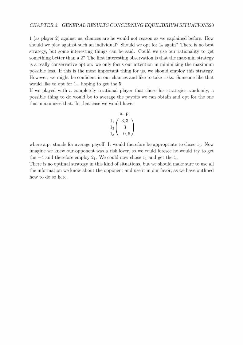
1 (as player 2) against us, chances are he would not reason as we explained before. Howshould we play against such an individual? Should we opt for 12 again? There is no beststrategy, but some interesting things can be said. Could we use our rationality to getsomething better than a 2? The first interesting observation is that the max-min strategyis a really conservative option: we only focus our attention in minimizing the maximumpossible loss. If this is the most important thing for us, we should employ this strategy.However, we might be confident in our chances and like to take risks. Someone like thatwould like to opt for 11, hoping to get the 5.If we played with a completely irrational player that chose his strategies randomly, apossible thing to do would be to average the payoffs we can obtain and opt for the onethat maximizes that. In that case we would have:
a. p.
11 3, 3
12 3
13 −0, 6
where a.p. stands for average payoff. It would therefore be appropriate to chose 11. Nowimagine we knew our opponent was a risk lover, so we could foresee he would try to getthe −4 and therefore employ 21. We could now chose 11 and get the 5.There is no optimal strategy in this kind of situations, but we should make sure to use allthe information we know about the opponent and use it in our favor, as we have outlinedhow to do so here.

Chapter 4
Mixed Extensions of Matrix Games
In such games where maxi minj aij 6= minj maxi aij, no equilibrium situation will bereached. This won’t satisfy the players, and, if the game is repeated, they may try tochange their strategy in order to increase their payoff. Let’s assume now that the playerswill chose their strategy among the si ∈ Sni
i1 with a certain frequency. The determination
of a mixed strategy consists in assigning a probability xi to every strategy si ∈ Snii , so
xi = P (Y = si), where Y is the strategy it is picked. This can be thought as a probabilitydistribution X that:
X = (x1, ..., xni) xi ≥ 0
ni∑i=1
xi = 1
If Iniis the ni-vector (1, ..., 1), we can summarize the last condition to XITni
= 1. Thetotality of all vectors (x1, ..., xni
) form a ni-dimensional Euclidian space Eni . However,these are subject to conditions xi ≥ 0 and
∑ni
i=1 xi = 1. Taking that into account, itis easy to see that the set of these resulting vectors is a (ni − 1)-dimensional simplexsubmerged in Eni . We will call this set, the one of all possible mixed strategies over Sni
i ,as Sni
i , and we will denote a mixed strategy by X ∈ Snii . In the case of ni = 2, for
example, S2i is the segment that joins (1, 0) to (0, 1). The fact that
∑ni=1 xi = 1 trivially
tells us that Snii is bounded. The simplex Sni
i is clearly a subset of a hyperplane of Eni .It is easy to see that is closed and it follows that Sni
is therefore compact.
4.1 Mixed Extension of a game
With a clever trick, we can transform an antagonistic game where players use mixedstrategies to a normal game. Let A = (aij) be the matrix of the matrix game Γ =
〈S1, S2, H1〉.
Definition. A pair (X, Y ) ∈ S1 × S2 of mixed strategies is called a situation in mixedgames.
1From now on, for the sake of clarity, we will always make explicit the cardinal ni of Si, so Snii will
mean the set of ni available strategies to player i.
21

CHAPTER 4. MIXED EXTENSIONS OF MATRIX GAMES 22
Every situation (i, j) (in the common usage) is a random event that occurs now witha certain probability xiyj. In such situation the payoff aij is obtained. We can easilycompute the average payoff when X and Y are employed as:
H1(X, Y ) =m∑i=1
n∑j=1
aijxiyj = XAY T
So basically now we can assign a precise payoff to every situation in mixed strategiesbecause we have eliminated the probabilistic nature of the strategies. Given that weare using the expected value, the Law of Large Numbers accounts for why the followinganalysis will works when the game is repeated a lot of times. Therefore a good strategymight give bad results in an isolated realization of the game.
Definition. A mixed extension of the game Γ = 〈S1, S2, H1〉 is the antagonistic gameΓ = 〈S1, S2, H1〉.
As condition (2.1) claims, for a general antagonistic game Γ = 〈S1, S2, H1〉, a situation(s∗1, s
∗2) ∈ S1 × S2 will be an equilibrium situation of Γ iff (s∗1, s
∗2) is a saddle point of
H1(s1, s2). If we apply this result to the antagonistic game Γ = 〈S1, S2, H1〉, we deducethat a situation (X∗, Y ∗) ∈ S1 × S2 will be an equilibrium situation of Γ if (X∗, Y ∗) is asaddle point of the function H(X, Y ). We know then that a situation (X∗, Y ∗) ∈ S1× S2
is an equilibrium situation / saddle point iff:
XAY ∗T ≤ X∗AY ∗T ≤ X∗AY T ∀(X, Y ) ∈ S1 × S2
We will see that for any matrix game Γ with matrix A there exists an equilibrium situation(X∗, Y ∗) in the mixed extension of the game Γ. As we saw in Theorem 3.2, to prove sowe have to verify that maxX minY XAY
T and minY maxX XAYT 2 exist and are equal.
Lemma. For any Y ∈ S2 and a s.t.
Ai·YT ≤ a ∀i
then ∀x ∈ S1 we have that XAY T ≤ a. Similar results for the inequalities of the formAi·Y
T ≥ a, XA·j ≤ a and XA·j ≥ a follow.
Proof. Clearly, as xi ≥ 0 ∀i:
Ai·YT ≤ a =⇒ xiAiY
T ≤ xia
It readily follows that:
XAY T =∑i
xiAi·YT ≤
∑i
xia = a∑i
xi = a
2For matrix games, given that X = (1−x, x) and Y = (1− y, y), to maximize and minimize for everyvector, i.e., to compute for example maxX minY XAY
T , is the same as to compute maxxminyXAYT .

CHAPTER 4. MIXED EXTENSIONS OF MATRIX GAMES 23
Theorem 4.1. Let Γ be the mixed extension of a game Γ. Then (X∗, Y ∗) ∈ S1 × S2 isan equilibrium situation of Γ iff Ai·Y
∗T ≤ X∗AY ∗T ≤ X∗A·j
Proof. The necessity is trivial, as this is a particular case of XAY ∗T ≤ X∗AY ∗T ≤X∗AY T for X = 1i and Y = 1j, where the notation should be clear. Let’s prove thesufficiency. To do so, let’s call X∗AY ∗T = a. We just proved that:
Ai·Y∗T ≤ a =⇒ XAY ∗T ≤ a
X∗A·j ≥ a =⇒ X∗AY T ≥ a
and then clearly XAY ∗T ≤ X∗AY ∗T ≤ X∗AY T . �
Existence of maxX minY XAYT and minY maxX XAY
T
Lemma. Let Γ be the mixed extension of a game Γ. For any Y0 ∈ S2 there exists themaxxXAY
T0 and for any X0 ∈ S1 there exists the minyX0AY
T .
Proof. It is clear that:
XAY T0 =
∑i
xiAi·YT0 ≡ linear function f(xi)
Given that S1 is a compact set (it is trivially closed and it is bounded because we aredealing with matrix games) then the maximum clearly exists. The other statement isproved analogously.
Lemma. Let Γ be the mixed extension of a game Γ. For any X0 ∈ S1 there exists j0(X0)
s.t.minyX0AY
T = X0A·j0
and for any Y0 ∈ S2 there exists i0(Y0) s.t.
maxx
XAY T0 = Ai0·Y0
Proof. Consider {X0A·j}j and let X0A·j0 be the smallest element in the set. Then giventhat:
X0A·j0 ≤ X0Aj ∀j =⇒ X0A·j0 ≤ X0AYT ∀Y ∈ S2
Given that this inequality is valid ∀Y ∈ S2, using the definition of minimum we canconclude that:
X0A·j0 ≤ minyX0AY
T
At the same time, X0A·j0 is a particular case of X0AYT (for Y = 1j) so it’s also true
that:X0A·j0 = X0A1T
j ≥ minyX0AY
T
and the result follows. The demonstration of maxxXAYT0 = Ai0·Y
T0 would be carried
out analogously.

CHAPTER 4. MIXED EXTENSIONS OF MATRIX GAMES 24
Lemma. The y-function maxxXAYT and the x-function minyXAY
T are continuous
Proof. We are only going to prove the continuity of the first function, the other case isproven analogously. Given that maxxXAY
T = maxiAi·YT , we only need to prove that
maxiAi·YT is continuous. Ai·Y
T is obviously continuous in Y . Take ε > 0 and δ s.t.
for |Y ′−Y ′′| < δ =⇒ |Ai·Y′T−Ai·Y
′′T | < ε ⇐⇒ Ai·Y′′T−ε < Ai·Y
′T < Ai·Y′′T+ε ∀Y ′, Y ′′
Recall that if f(Y ′) > f(Y ′′) ∀Y ′, Y ′′ then max f(Y ′) > max f(Y ′′) and so it follows that:
maxiAi·Y
′′T − ε < maxiAi·Y
′T < maxiAi·Y
′′T + ε =⇒ |maxiAi·Y
′T −maxiAi·Y
′′T | < ε
Theorem 4.2. The quantities maxX minY XAYT and minY maxX XAY
T exist.
Proof. It has just been proven that maxX XAYT is a continuous function of Y , which
is defined in S2, which, as was discussed, is a compact set and hence the minimum istrivially attained. The other result is proven analogously. �
Convex Sets
Definition. In an euclidian space En, a certain S ⊂ En is called a convex subset of En
if ∀ U, V ∈ S and ∀λ ∈ [0, 1] then
λU + (1− λ)V ∈ S
i.e. the whole segment going from any point of the subset to some other one is also partof the subset.
Lemma. (cf.[8]) If A is a closed convex set and x ∈ En\A, then A and x can be separatedby a hyperplane.
Lemma. For any matrix A one of this two options holds:
1. There exists a vector X ∈ Sm1
3 s.t. XA·j ≥ 0 ∀j
2. There exists a vector Y ∈ Sn2 s.t. Ai·Y
T ≤ 0 ∀i
Proof. Recall that Sm1 is the (m− 1)-simplex. The convex hull or convex envelope of a
set S, i.e., the smallest possible convex set C that contains it, can be expressed as:
C(S) =
{#S∑i
αixi
}where xi ∈ S, αi > 0 ∀i, and
#S∑i
αi = 1
Let’s consider the convex envelope of Sm1 and A·j. There are two possibilities: ~0 ∈
C(Sm1 ∪ A·j) or ~0 /∈ C(Sm
1 ∪ A·j).3Bear in mind that we are using again the notation explained in the first footstep of this chapter.

CHAPTER 4. MIXED EXTENSIONS OF MATRIX GAMES 25
• If ~0 ∈ C(Sm1 ∪A·j), applying the definition of convex hull it follows that there exist
certain {αj}j and {ηi}i s.t.
n∑j=1
αjA·j +m∑i=1
ηisi = ~0 with αi > 0, ηi > 0 and∑j
αj +∑i
ηi = 1
The above expression can be written as∑bisi = ~0, and therefore:
bi =n∑
j=1
αja·j + ηi = 0
and given that ηi > 0 ∀i it follows that∑n
j=1 αja·j ≤ 0. The quantity α =∑n
j αj
is positive. It is clearly nonnegative, and if it was 0 it would follow that αj = 0 ∀j,what would mean using the expression above that ηi = 0, something which wouldcontradict
∑j αj +
∑i ηi = 1. We can therefore define yj = αj/α. Given that
yj ≥ 0 ∀j and∑
j yj = 1, Y = (y1, ..., yn) could be thought as a mixed strategy, i.e.,as an element of Sn
2 . If we use now the expression∑n
j=1 αja·j ≤ 0 and we divide itfor α, the desired result follows:
n∑j=1
yjaij = Ai·YT ≤ 0 ∀i
• For ~0 /∈ C(Sm1 ∪ A·j), we can apply the previous lemma4 to find that ~0 can be
separated from C by a hyperplane, which we will assume to go through the point~0. Let V z = 0 be its equation. Without any loss of generality, we can assume that:
V Z > 0 ∀z ∈ C(Sm1 ∪ A·j)
In particular, for any pure strategy, it follows that V si = vi > 0 and let’s callv =
∑vi. It is time we considered now
X =(v1v, ...,
vnv
)The same arguments that justified in the previous case that Y was a mixed strategyapply here to show that X ∈ Sm
1 . Consider now:
Xz =
(∑i
1
vvi
)zi =
1
vV z ≥ 0 ∀z
apply this to the vectors A·j and the result readily follows.4It can be proved that the convex hull of a compact set is closed.

CHAPTER 4. MIXED EXTENSIONS OF MATRIX GAMES 26
4.1.1 The MinMax Theorem
Theorem 4.3. (The MinMax Theorem) For any matrix A and for any (X, Y ) ∈ S1× S2
the equality:maxX
minYXAY T = min
YmaxX
XAY T
holds.
Proof. We apply to A the previous lemma. Let’s assume first the first option, i.e.XA·j ≥ 0 ∀j. As it is clear now:
XA·j ≥ 0 ∀j =⇒ X0AYT ≥ 0 ∀j ∀Y ∈ S2
As this is valid for every Y ∈ S2, then
minYX0AY
T ≥ 0 =⇒ maxX
minYXAY T ≥ 0
The second option, Ai·YT ≤ 0 ∀i, leads, proceeding analogously, to minY maxX XAY
T ≤0. One of the two inequalities must hold, so it is impossible that:
maxX
minYXAY T < 0 < min
YmaxX
XAY T
If A = (aij), consider A(t) = (aij − t). Now:
XA(t)Y T =∑i
∑j
xi(aij − t)yj =∑i
∑j
xiaijyj − t∑i
∑j
xiyj = XAY T − t
It is impossible that:
maxX
minY
(XAY T−t) < 0 < minY
maxX
(XAY T−t) =⇒ maxX
minYXAY T < t < min
YmaxX
XAY T
And therefore, it is impossible that maxX minY XAYT < minY maxX XAY
T so it mustalways be maxX minY XAY
T ≥ minY maxX XAYT . However, according to Theorem
3.1, and applying it to a matrix game, it must always hold that maxX minY XAYT ≤
minY maxX XAYT , so the only way both things can be true is if:
maxX
minYXAY T = min
YmaxX
XAY T
�
Just as it happened for non-repeated games, player 1 is inclined to choose the strategythat accomplishes v1 = maxi minj XAY
T and player 2 the strategy that accomplishesv2 = minj maxiXAY
T . But now, the equivalent of this expressions, as it has just beenproven, will always be equal, i.e. v′1(A) = v′2(A) 5 always! This means that if bothplayers behave rationally the game will always end up in this situation. Mixed extensionsof matrix games are therefore predetermined and that’s why they are called completelydetermined games.
5where by analogy v′1(A) = maximinj XAYT and v′2 = minj maxiXAY
T

CHAPTER 4. MIXED EXTENSIONS OF MATRIX GAMES 27
Definition. Let Γ be the mixed extension of the matrix game Γ. We define the value ofthe game (and bear in mind it only makes sense in mixes strategies) as:
v(A) = maxX
minYXAY T = min
YmaxX
XAY T
or in a shorter way v(A) = v′1(A) = v′2(A). Notice that v(A) tells us the mean gainplayer 1 will get, as long as they both employ their max-min strategies. Trivially then:v(A) = H1(X
∗, Y ∗). To solve a game is to determine the value of the game and themin-max strategies.
4.1.2 First Example
It is time now we talked about how to find equilibrium situations in mixed strategies. Thefirst thing it should be said is that this has already been done in the first chapter of thisundergraduate thesis. Let’s give now a more precise explanation of how we proceeded.To do so, let’s focus our attention on the example 2 of section 3.2.1. We had a game withmatrix A for which there was no equilibrium situation. We know now that, in mixedstrategies, it must have at least one equilibrium situation. Let’s assume each player picksa general mixed strategy, i.e. X = (1− x, x) and Y = (1− y, y) 6.
( 1− y y
1− x 4 2
x 0 3
)We therefore have that:
H(X, Y ) =m∑i=1
n∑j=1
aijxiyj = 4(1− x)(1− y) + 2(1− x)y + 3xy = 5xy − 2y − 4x+ 4
Now we want to compute:
max0≤x≤1
min0≤y≤1
5xy−2y−4x+ 4 = max0≤x≤1
miny∈{0,1}
5xy−2y−4x+ 4 = max0≤x≤1
min{−4x+ 4, x+ 2}
where we have used Theorem 1.1 in the first equality. The function H(x) = min{−4x+
4, x+ 2} is graphed in figure 4.1.It can readily be checked that it attains its maximum at x∗ = 2/5 and thus:
v(A) = v′I(A) =2
5+ 2 = 2.4
If we want to know now the strategy player 2 should employ we only need to compute:
min0≤y≤1
max0≤x≤1
5xy − 2y − 4x+ 4 = min0≤y≤1
maxx∈{0,1}
5xy − 2y − 4x+ 4 = min0≤y≤1
max{−2y + 4, 3y}
6This is arbitrary and we could have perfectly taken X = (x, 1− x) and Y = (y, 1− y). We warn thereader that we will alternate between these throughout the following chapters.

CHAPTER 4. MIXED EXTENSIONS OF MATRIX GAMES 28
0 0.2 0.4 0.6 0.8 1
0
0.5
1
1.5
2
2.5
x
H(x)
Figure 4.1: Graph of min{−4x+ 4, x+ 2}
The minimum of max{−2y+4, 3y} is attained when y∗ = 4/5 and it obviously yields 2.4.We have solved the game:
min-max strategy X∗ =
(3
5,2
5
)max-min strategy Y ∗ =
(1
5,4
5
)value of the game v(A) =
12
5= 2.4
Both this and the bomber game were matrix games with 2×2-matrixes, i.e. n1 = #Sn11 =
2 and also n2 = 2. Let us say at this point that there is no easy algorithm to solve n×mgames. Everything that can be said is that a Nash Equilibrium will always exist in mixedstrategies. However, let’s try to go beyond 2× 2 games by studying 2×m games
4.1.3 Two lemmas
Definition. Let Γ be a game with matrix A = (aij). Then a row i dominates over rowk if aij ≥ akj ∀j and column j dominates over column l if aij ≤ ail ∀i. Intuitively, adominated row is not interesting for player 1 and a dominated column is not interestingfor player 2, so given that the players are not going to pick them, we can remove themfrom the game. Let’s prove it.
Lemma. If either a dominated row or column is removed from the matrix A, the solutionof the remaining game is the same as the one of the original game.
Proof. Let Γ = 〈S1, S2, H1〉 be a matrix game and Γ = 〈S1, S2, H1〉 its mixed extension.Let the second strategy of player 1 dominate over the first one. Consider thus the gamesΓ′ = 〈S ′1, S2, H1〉 and Γ′ = 〈S ′1, S2, H1〉 where clearly S ′1 = {X ∈ S1 s.t. x1 = 0}. Let

CHAPTER 4. MIXED EXTENSIONS OF MATRIX GAMES 29
(X ′∗, Y ′∗) be the optimal strategies of Γ′. Are these the optimal strategies of Γ as well?Let v′ be the value of Γ′. This means that:
H1(X′∗, Y ′) ≥ H1(X
′∗, Y ′∗) = v′ ∀Y ′ ∈ S2
H1(X′, Y ′∗) ≤ H1(X
′∗, Y ′∗) = v′ ∀X ′ ∈ S ′1
In order to prove the lemma, we want to check if:
H1(X′∗, Y ′) ≥ v′ ∀Y ′ ∈ S2
H1(X′, Y ′∗) ≤ v′ ∀X ′ ∈ S1
what will mean that v′ is also the value of the game Γ. The first inequality is triviallytrue. When it comes to the second:
H1(X′, Y ′∗) =
n∑i
m∑j
x′iaijy′∗j = x′1
m∑j
a1jy′∗j +
n∑i=2
m∑j=1
x′iaijy′∗j ≤ (domination)
≤ x′1
m∑j=1
a2jy′∗j +
n∑i=2
m∑j=1
x′iaijy′∗j = H1(X ′, Y
′∗) ≤ v ∀X ′ ∈ S1
where we used that X ′ = (0, x1 + x2, x3, ..., xn) ∈ S ′1. �
Definition. A pure strategy is said to be relevant if it is employed with probabilitygreater than zero in a max-min strategy.
Lemma. Any relevant strategy played against a max-min strategy yields the value ofthe game.
Proof. Let Γ = 〈S1, S2, H1〉 be a matrix game and Γ = 〈S1, S2, H1〉 its mixed extension.Let X∗ = (x∗1, ..., x
∗k, 0, ..., 0) (x∗i 6= 0 i < k) and Y ∗ be the max-min strategies. Then:
v = H1(X∗, Y ∗) =
∑i
∑j
x∗i aijy∗j =
k∑i
x∗i H1(1i, Y∗) =⇒
k∑i
x∗iH1(1i, Y
∗)
v= 1
We know that∑
i x∗i = 1. Recall that v = v′2, so given that player 2 is employing a
max-mix strategy we have that H1(1i,Y∗)
v′2≤ 1 ∀i ≤ k. In fact, these inequalities will turn
out to be equalities. If H1(1i,Y∗)
v< 1 for some i and the others were equal to 1, we would
have: ∑i
x∗iH1(1i, Y
∗)
v<∑i
x∗i = 1
which can’t be true. Therefore:
H1(1i, Y∗)
v= 1 ∀i ≤ k =⇒ H1(1i, Y
∗) = v ∀i ≤ k
�

CHAPTER 4. MIXED EXTENSIONS OF MATRIX GAMES 30
In the example of section 4.1.2, we found that all strategies were relevant and that thevalue of the games was 12/5. We can thus check the validity of the lemma:(
1 0
0 1
)(4 2
0 3
)(1545
)=
(125125
)&
(3
5,2
5
)(4 2
0 3
)(1 0
0 1
)=
(12
5,12
5
)which obviously turns out to be right.
4.1.4 2×m games
Let’s assume we have a game Γ = 〈S1, S2, H1〉 with matrix A where #S1 = 2 and#S2 = m. Also let’s assume no saddle point exists (otherwise we don’t need mixedstrategies to solve the game). We can solve these games by:
1. Using the domination lemma.
2. Finding relevant strategies.
3. Using the relevant strategies lemma to find the max-min strategies.
Let’s see how this works with an example:(1 7 5 3
8 2 6 4
)We apply 1) and we are left with: (
1 7 3
8 2 4
)Now let’s move to 2). We assume a strategy X = (x, 1− x) for player 1 and we confrontit all the pure strategies of player 2 (21 = (1, 0, 0), 22 = (0, 1, 0) and 23 = (0, 0, 1)). Wedo that because if X is a max-min strategy, we know that we only need to confront itagainst all the pure strategies to obtain the value of the game. We thus have:
The combination of X with 21 yields: r1(x) = x+ 8(1− x) = −7x+ 8
The combination of X with 22 yields: r2(x) = 7x+ 2(1− x) = 5x+ 2
The combination of X with 23 yields: r3(x) = 3x+ 4(1− x) = −1x+ 4
Figure 4.2 a) shows the graph of these functions.Player 1, as always, will choose the strategy that accomplishes max min{−7x + 8, 5x +
2,−x + 4}. See figure 4.2 b), where the function f(x) = min{−7x + 8, 5x + 2,−x + 4}is represented. The maximum (the value of the game), which lays somewhere betweenx = 0.2 and x = 0.4, comes from the intersection of r2(x) and r3(x). Provided that r1(x)
can’t yield the value of the game and applying the relevant strategies lemma, we concludethat 21 is an irrelevant strategy, so it can be removed. As a consequence, we are left with:(
7 3
2 4
)

CHAPTER 4. MIXED EXTENSIONS OF MATRIX GAMES 31
0 0.2 0.4 0.6 0.8 1
2
4
6
8
x
ri(x)
a)
0 0.2 0.4 0.6 0.8 1
1
2
3
x
f(x)
b)
Figure 4.2: a) Graph of r1(x), r2(x) and r3(x). b) Graph of min{r1(x), r2(x), r3(x)}
Let X∗ = (x∗, 1−x∗) be the max-min strategy of player 1. The relevant strategies lemmaasserts that:
(x∗, 1− x∗)(
7 3
2 4
)(1
0
)= v & (x∗, 1− x∗)
(7 3
2 4
)(0
1
)= v
From these equations we conclude that: 5x∗ + 2 = −x∗ + 4 and therefore x∗ = 1/3 andv = 11/3. At the same time:
(1, 0)
(7 3
2 4
)(y∗
1− y∗
)= v =
11
3
from where we deduce that: 4y∗ + 3 = 11/3 and therefore y∗ = 1/6. We have solved thegame:
min-max strategy X∗ =
(1
3,2
3
)max-min strategy Y ∗ =
(1
6,5
6
)value of the game v(A) =
11
3= 3.67

Chapter 5
General Noncooperative Games
Let us study now those noncooperative games where there are more than two players.We have seen so far how all matrix games have at least one equilibrium situation inmixed strategies. This interesting result can be generalized into a much more powerfulstatement, originally proved by Nash, that we present now and will be proved later.
Nash’s Theorem. In any noncooperative game there is at least one equilibrium situationin mixed strategies.
5.1 Mixed Extensions of Noncooperative Games
Let Γ = 〈I, {Si}i∈I , {Hi}i∈I〉 be a noncooperative game and let’s assume that #{Si} <+∞ ∀i. Let σi denote the mixed strategy of player i. We could think of σi as aprobability distribution that assigns to every strategy si ∈ Si the probability of beingactually employed: σi(si). If player i decides to pick the same strategy si every time, i.e.to pick a pure strategy, clearly σi(si) = 0 ∀si 6= si and σi(si) = 1. The set of all mixedstrategies of player i will be denoted by Si. The probability distributions will be assumedto be independent, so the probability of arriving at the situation s ∈ S will be:
σ(s) = σ(s1, ..., sn) = σ1(s1) · · ·σn(sn)
The set of all this probability distributions will be now the set of situations. To definethe payoff of this new situations, we will proceed as we did for the mixed extension ofmatrix games, i.e. averaging the payoff of every pure strategy.
Hi(σ) =∑s∈S
Hi(s)σ(s) =∑s1∈S1
· · ·∑sn∈Sn
H(s1, ..., sn)n∏
i=1
σi(si)
Clearly now we can define the mixed extension of the game Γ = 〈I, {Si}i∈I , {Hi}i∈I〉 as:
Γ = 〈I, {Si}i∈I , {Hi}i∈I〉
32

CHAPTER 5. GENERAL NONCOOPERATIVE GAMES 33
Theorem 5.1. For any situation σ, there is at least one pure strategy s0i ∈ Si ∀i s.t.
σi(s0i ) > 0 (It is sometimes employed) & Hi(σ||s0i ) ≤ Hi(σ)
Proof. We are going to proceed with a reductio ad absurdum. Suppose no such strategyexists. Then, all pure strategies si of player i that satisfy σi(s0i ) > 0 must satisfy as well:
Hi(σ||si) > Hi(σ)
As for these strategies σi(si) > 0, we can readily state that Hi(σ||si)σi(si) > Hi(σ)σi(si).For those si ∈ Si that are never employed (σi(si) = 0) it holds that Hi(σ||si)σi(si) =
Hi(σ)σi(si) = 0. Clearly: ∑si∈Si
Hi(σ||si)σi(si) >∑si∈Si
Hi(σ)σi(si)
from where it follows that Hi(σ) > Hi(σ), which is a contradiction. �
Analogously as we have done before, we will say that σ∗ ∈ S is an equilibrium situationin Γ if:
Hi(σ∗||σ′i) ≤ Hi(σ
∗) ∀σ′i ∈ Si ∀i ∈ I
Let’s derive now a result we will use to prove Nash’s Theorem.
Theorem 5.2. A necessary and sufficient condition for a situation σ∗ in Γ to be anequilibrium situation is that:
Hi(σ∗||s′i) ≤ Hi(σ
∗) ∀s′i ∈ Si ∀i ∈ I (5.1)
Proof. First of all, what is Hi(σ∗||s′i)? Clearly, as we said before, σi(si) = δ(si=s′i)
sousing the expression for Hi(σ) it’s easy to see that:
Hi(σ∗||s′i) =
∑s1∈S1
· · ·∑
si−1∈Si−1
∑si+1∈Si+1
· · ·∑sn∈Sn
H(s1, ..., si−1, s′i, si+1, ..., sn)
n∏i=1i 6=j
σi(si)
The statement (5.1) is a particular case of the definition of equilibrium situation. Let’sfocus on the necessity. Let’s assume the validity of (5.1) and let’s choose an arbitrarystrategy σi ∈ Si. We have that:
Hi(σ∗||s′i) ≤ Hi(σ
∗) ⇐⇒ Hi(σ∗||s′i)σi(s′i) ≤ Hi(σ
∗)σi(s′i)
Trivially: ∑s′i∈Si
Hi(σ∗||s′i)σi(s′i) ≤
∑s′i∈Si
Hi(σ∗)σi(s
′i) = Hi(σ
∗)∑s′i∈Si
σi(s′i) = Hi(σ
∗)

CHAPTER 5. GENERAL NONCOOPERATIVE GAMES 34
But:
∑s′i∈Si
Hi(σ∗||s′i)σi(s′i) =
∑s′i∈Si
∑s1∈S1
· · ·∑
si−1∈Si−1
∑si+1∈Si+1
· · ·∑sn∈Sn
H(s||s′i)n∏
i=1i 6=j
σi(si)
σi(s′i) =
=∑s1∈S1
· · ·∑si′∈Si
· · ·∑sn∈Sn
H(s||s′i)
n∏i=1i 6=j
σi(si)
σi(s′i) = Hi(σ
∗||σi)
and the result follows.
5.2 Nash’s Theorem
Theorem 5.3. (Brower’s Fixed Point Theorem) (cf.[5]) For any continuous function f
mapping a compact convex set into itself there is a fixed point, i.e. a point x0 such thatf(x0) = x0.
Theorem 5.4. (Nash’s Theorem) In any noncooperative game Γ = 〈I, {Si}i∈I , { Hi}i∈I〉there is at least one equilibrium situation in mixed strategies.
Proof. Every player has available a set of pure strategies Smii . The set Smi
i is the setof mixed strategies. Geometrically, as previously discussed, it’s a (mi − 1)-simplex. Anysituation σ = (σ1, ..., σn) can be seen as a point of the cartesian product Sm1
1 × ...× Smnn .
This is a convex closed subset of the (m1 + ... + mn − n)-euclidean space. For anysituation σ and for any pure strategy of any player, ∀sji ∈ Si (it should understood asthe jth strategy of player i) let’s define
φij(σ) = max{0, Hi(σ||si)− Hi(σ)} ≥ 0
For a fixed situation σ, we are calculating the increase of payoff when we change σi by apure strategy sji . Let’s define now, ∀i and ∀j:
σi(sji ) + φij(σ)
1 +∑mi
j=1 φij(σ)
where σi(sji ) is the probability of employing sji , so it’s a nonnegative value. So is φij(σ)
and consequently the fraction is always positive. Clearly:
mi∑j=1
σi(sji ) + φij(σ)
1 +∑mi
j=1 φij(σ)=
∑mi
j=1 σi(sji ) +
∑mi
j=1 φij(σ)
1 +∑mi
j=1 φij(σ)=
1 +∑mi
j=1 φij(σ)
1 +∑mi
j=1 φij(σ)= 1
For a fixed situation σ and for a fixed player i, the elements of{σi(s
ji ) + φij(σ)
1 +∑mi
j=1 φij(σ)
}j

CHAPTER 5. GENERAL NONCOOPERATIVE GAMES 35
given that are positive and add up to one, could be thought as forming a mixed strategy.As this can be done for every player, we would have a mixed strategy for every playerand thus a situation. Therefore, given a situation σ we can define a new situation f(σ)1
the way we have explained. To be able to apply Brower’s fixed theorem, we need tocheck if f is continuous. Is φij(σ) a continuous function of σ? Clearly max{0, x}, Hi(σ)
and the rest function are continuous and provided that the composition of continuousfunctions is a continuous function the result follows. At the same time, the probabilitydistribution σi(sji ) is also continuous on σ and therefore the numerator is continuous. Thesame arguments show that the denominator is always continuous and given that it nevervanishes, f is a continuous function. All the requirements to apply the Brower FixedTheorem hold so we conclude that there exists at least one σ0 s.t. f(σ0) = σ0. In otherterms:
σ0i (sji ) =
σ0i (sji ) + φij(σ
0)
1 +∑mi
j=1 φij(σ0)
According to Theorem 5.1, for every player and applied to the situation σ0, there existsa pure strategy s0i ∈ Si s.t. σi(s0i ) > 0 and φi0(σ
0) = 0. For this particular strategy, theexpression above reads as:
σ0i (s0i ) =
σ0i (s0i )
1 +∑mi
j=1 φij(σ0)
from where it follows that∑mi
j=1 φij(σ0) = 0. Recalling that φij(σ) = max{0, Hi(σ||si)−
Hi(σ)} ≥ 0 it is clear that:
φij(σ0) = 0 ∀i∀j =⇒ Hi(σ
0||sji ) ≤ Hi(σ0)
and applying Theorem 5.2 we deduce that σ0 is a Nash Equilibrium. �
Remark. This important theorem is what allows us to say that there always exists, atleast, one Nash equilibrium. However, it is not a constructive theorem, so it doesn’t tellus how to find such equilibrium situations. This comes from the fact that Brower’s fixedtheorem, the basis of our demonstration, is not constructive either because it does notexplain how to find the fixed points.
In noncooperative games, not all the players have the same payoff at all equilibriumsituations. For general noncooperative games, there is no optimal strategy that yieldsthe value of the game, because there is no value of the game, only one or more Nashequilibriums. Also, assuming that every player knows which of his strategies can yieldan equilibrium situation, only certain combinations of these strategies will in the endactually lead to a Nash equilibrium. Let us illustrate this with some examples.
1f : S1 × ...× Sn −→ S1 × ...× Sn and clearly f(σ) = σi(sji )+φij(σ)
1+∑mi
j=1 φij(σ)

CHAPTER 5. GENERAL NONCOOPERATIVE GAMES 36
5.3 Examples
In general noncooperative games, we can also speak of v1 = maxX minY H1(X, Y ) andv2 = maxY minX H2(X, Y ) 2. They represent, clearly, the minimum gain each player canassure. As such, we can define the max-min solution (X∗, Y ∗) formed by those strategiesthat satisfy the previous equalities. Every time we do that, we are assuming a zero-sum game for every player. However, now the players do not necessarily have oppositemotivations, i.e., the players gain does not come from the opponent’s loss as in zero-sumgames. This will mean that H1(X
∗, Y ∗) and H2(X∗, Y ∗) are not going to be necessarily
equal to v1 and v2. So even if we can define a max-min solution, this will not correspondto an equilibrium situation. Let’s illustrate this with an example.
5.3.1 The gender war
A couple is discussing what to do this evening. The guy, who is passionate about cinema,wants to go to the movies whereas the girl, a big tennis fan, wants to stay in and watch amatch on TV. Even if they have opposite preferences, both of them prefer to do somethingtogether. If 11 and 21 stand for going to the cinema and 12 and 22 for staying in, we canwrite: ( 21 22
11 (1, 4) (0, 0)
12 (0, 0) (4, 1)
)where it is clear which player is the guy and which the girl. Let’s find the max-minsolution for the girl. We assume a zero-sum game and therefore have:
( y 1− yx 1 0
1− x 0 4
); H1 = 5xy− 4x− 4y+ 4 =⇒ v1 = max
xminy
(5xy− 4x− 4y+ 4) =4
5
This is attained at x∗ = 45and the max-min strategy for the girl therefore is X∗ = (4
5, 15).
Analogously for the boy we have that Y ∗ = (15, 45) and v2 = 4
5. If this were the strategies
they actually picked, 1625
of the times we would end up with the outcome (0, 0). There aretwo evident equilibrium situations, which are: (11, 21) and (12, 22). Are there any more?To answer the question, let’s explain a method to find Nash equilibriums in 2× 2 games.
5.3.2 The swastika method
Let’s assume general strategies (X, 1−X) and (Y, 1− Y ) for our players. A equilibriumsituation is an admissible situation for every player. We are going to calculate separatelyfor every player the admissible situations and we will then intersect them. Let’s focus on
2If H2 = −H1 we have that vII = maxY minX −H1 = −minY maxX H1 which corresponds to thedefinition we gave of vII for matrix games with a minus sign in front. This is because before we spokeof the loss of player 2 whereas now we talk about his gain.

CHAPTER 5. GENERAL NONCOOPERATIVE GAMES 37
player 1. For any strategy his opponent picks, i.e. for any Y , we are going to calculatethe best reply which yields maxX H1(X, Y ). Let’s pick the same matrix as in the genderwar. Starting with H1 we have:
( y 1− yx 1 0
1− x 0 4
); H1 = x(5y − 4)− 4y + 4
The part that player 1 can alter is the one that depends on x. The maximum of theexpression above, given that it is linear on x, is either attained at x = 0 or at x = 1.Also, there is the option that the linear term vanishes. All in all, to maximize H1:
• if y < 45, then player 1 should set x = 0.
• if y = 45, then the maximum is attained for any x.
• if y > 45, then player 1 should set x = 1.
If we adopt now player’s 2 perspective, for him:
( y 1− yx 4 0
1− x 0 1
); H2 = y(5x− 1)− x+ 1
and proceeding analogously:
• if x < 15, then player 2 should set y = 0.
• if x = 15, then the maximum is attained for any y.
• if x > 15, then player 2 should set y = 1.
We can graph all this (see figure 5.1) and we find three equilibrium situations:
(X∗, Y ∗) = ((0, 1), (0, 1)) . Then H1(X∗, Y ∗) = 4 and H2(X
∗, Y ∗) = 1
(X∗, Y ∗) = ((1, 0), (1, 0)) . Then H1(X∗, Y ∗) = 1 and H2(X
∗, Y ∗) = 4
(X∗, Y ∗) =
((1
5,4
5
),
(4
5,1
5
)). Then H1(X
∗, Y ∗) =4
5and H2(X
∗, Y ∗) =4
5
First of all, it is important to remark that the Nash Equilibriums yield different payoffsfor the players, something that illustrates that the concept of the value of the game hasno sense in general noncooperative games. Also, notice that the equilibrium points arenot interchangeable. See for example that (0, 1) is one of the strategies of player 1 thatyield a Nash equilibrium and so is (1, 0) for player 2. However, the combination of thesestrategies is not an equilibrium situation. As we said before, even if everybody knewwhich strategies yield Nash equilibriums, only certain combinations of these would infact actually lead to equilibrium situations.Could this method be generalized? or in other words: How can we solve a generalnoncooperative game? The answer is that nobody knows. The research of algorithms todo so is a very active topic of research nowadays.

CHAPTER 5. GENERAL NONCOOPERATIVE GAMES 38
0 0.2 0.4 0.6 0.8 1
0
0.2
0.4
0.6
0.8
1
(15 ,
45
)
(0, 0)
(1, 1)
x
y
Figure 5.1: Swastika method for the gender war
5.3.3 Prisoner’s Dilemma - First approach
Consider a 2× 2-game where S1 = S2 = {C,D} 3 with:
( C D
C (−12,−1
2) (−10, 0)
D (0,−10) (−6,−6)
)We can apply the Swastika Method to this game. Let’s see what happens. Proceedingas before, for player 1:
( y 1− yx −1
2−10
1− x 0 −6
); H1 = x
(7
2y − 4
)+ 6y − 6
The part that player 1 can alter is the one that depends on x. However, ∀y ∈ [0, 1] theterm (7
2y − 4) < 0. To maximize H1 player 1 should always set x = 0 regardless of the
value of y. If we do the same for player 2, we will have H2 = y(72x− 4
)+ 6x− 6, so the
same argument applies. Therefore, the only equilibrium situation is (D,D). But let’stake some perspective: This result is awful. Both player would be better off with (C,C),which, even if it is not an equilibrium situation, it is the best outcome of the game. Whatis going on here?
3The meaning of every strategy will be explained later.

Chapter 6
A Mathematical Explanation ofCooperation
The last chapter of this undergraduate thesis is of a different nature. Now we are goingto see how Game Theory can be used to help disciplines like Biology, Political Science,Law, Economy, etc. We are going to address a philosophical problem, known as the originof cooperation, that reads as follows: How can cooperation emerge in a world of selfishindividualistic people? As experience suggests, nowadays people normally pursue theirself interest, most of the times leaving no room for helping others. From a rational pointof view, there’s no point in helping strangers. Thomas Hobbes believed that, if left toa complete laissez faire, selfishness would compromise communal living and life wouldbecome "solitary, poor, nasty, brutish and short". To prevent this, he claimed that acentral authority, in the form of a state, was completely necessary. The debate, however,did not finish here, and the question of whether cooperation could emerge without the aidof a central supervision continued. In both the human race and animals, there are certainindividuals that challenge these pessimistic views on the human nature by showing clearsigns of altruism towards strangers. For example, is it known that during World WarOne, an admirable tactic agreement was made between the fighters of each side on thewestern front. Violating the orders of their superiors, the front-line soldiers kept fromshooting to kill as long as their enemies did the same, creating a pattern of cooperationthat benefited them all.Darwin, the father of the theory of evolution, was very aware of the need of cooperatingdispositions to perpetuate a species. As a consequence, he was concerned at the thoughtthat cooperation was destroyed by natural selection. As he himself explained:
"He who was ready to sacrifice his life [...] rather than betray his comrades, wouldoften leave no offspring to inherit his noble nature. The bravest men, who werealways willing to come to the front in war, and who freely risked their lives forothers, would on an average perish in larger numbers than other men. Therefore, ithardly seems probable that the number of men gifted with such virtues [...] could beincreased through natural selection, that is, by the survival of the fittest."
Charles Darwin, The Descent of Man. Part One, Chapter V.
39

CHAPTER 6. A MATHEMATICAL EXPLANATION OF COOPERATION 40
In the animal kingdom, where there is neither government nor law, theories such as theSelfish Gene, by Richard Dawkins, have been put forward to account for the presence ofcooperation. However, Game Theory can be used to prove the counterintuitive thesis thatpure self interest can lead to the emergence of cooperative dispositions towards strangers.To begin with, let’s take another look at the prisoner’s dilemma.
6.1 Prisoner’s Dilemma
Imagine that two burglars are caught red-handed breaking into a house but in accordancewith the need in a civilized world to keep within the legal frameworks, not enough validevidence is collected to find them guilty of an unlawful break-in. The intelligent policeofficers proceed to separate the suspected offenders and tell them the exact same thing.If you testify against your friend, you will be automatically released, and he will have toface a 10-year prison sentence. However, if your friend testifies against you too, you willalso be found guilty and both of you will face a 6-year prison sentence. If nobody saysanything, both of you will be accused of minor charges and will serve a 6 month sentence.The possible strategies are S1, S2 = {C,D}, C standing for Cooperate (with your partner)and D standing for Defect (your partner).
( C D
C (−12,−1
2) (−10, 0)
D (0,−10) (−6,−6)
)We saw in the previous chapter that there is only one equilibrium situation. We couldhave reasoned the following way to discover this: If your opponent cooperates, we comparea payoff of −1
2(when you cooperate) to a payoff of 0 (when you defect). If he doesn’t
cooperate we compare a payoff of −10 to a payoff of −6. This means, by definition, thatde situation (D,D) is an equilibrium situation. As we said before, this is an awful result,because it is clear that they would be better off cooperating. The prisoners dilemma,as an example of how the pursuit of self interest by each player leads to a bad outcomefor all, goes beyond the mere anecdotal story to raise a fundamental reflection regardinghuman cooperation. As we are going to see, the prisoner’s dilemma can shed some lighton why we cooperate with unknown individuals. To study this a bit better, let’s considera generic version of the game:
( C D
C (R,R) (S, T )
D (T, S) (P, P )
)where R is the reward for mutual cooperation, T is the temptation to defect, S is thesucker’s payoff and P the punishment for mutual defection 1. To encapsulate the problemswe want to deal with, we need to set T > R > P > S. In the repeated prisoner’s dilemma
1Where I am using Axelrod’s terms. See: [4]

CHAPTER 6. A MATHEMATICAL EXPLANATION OF COOPERATION 41
a second condition is added: 2R > T + S, which prevents the players to get out of thedilemma by exploiting each other. We want mutual cooperation to be a better optionthan betraying and being betrayed in turn.This game has served to show how cooperation can emerge in a world of selfish playerswhere there is no central authority. Is this, nevertheless, a good approximation of thereal world? Many philosophers have argued that human nature is entirely selfish. If wecare for others, they claim, it is because our own welfare resides in the welfare of others.This is not a very optimistic perspective of the human being but it is quite realistic. Ifwe adhere to this train of thought, our analysis would also apply to cooperation betweenfriends and family members. At the same time, nowadays we live in a society ruled bya central authority that forces us to cooperate (by prosecuting for failure to provide aidand assistance, for example), so someone could say our analysis would not apply to reallife. However, in most cases, like in the story that motivates the prisoner’s dilemma,cooperation is an option and not an obligation. But that’s not everything. Countries, forexample, do interact between each other without any supervision, and therefore topicslike the nuclear disarmament or the custom duties would also fall into this description.These situations are iterated versions of the prisoners dilemma. How should we play insuch case? Let’s assume we tell the players of the game that we are going to repeat thegame 20 times. Can cooperation emerge in this context? As we said, if the game is onlyplayed once, the optimal choice is to defect. Let’s then consider the last movement of ouriterated game. In that stage of the game, given that there will be no further encounterbetween the players, the wisest choice again is to defect. But bearing that in mind andgoing one step back in the game, we too should defect in the 19th move. Following thistrain of thought, we can deduce that the game is determined and its outcome is awful.What happens, though, if we never know how long the game is going to last for? Now,in every move, you have to think about the consequences your decisions might entail.To study this, the mathematician and political scientist Robert Axelrod organized acomputer prisoner’s dilemma tournament. He invited experts in the field to submit ideasof strategies, and he confronted 14 of them in total. It should be noted that no beststrategy exists regardless of the one your opponent employs. What it is clear is thatas long as you play against someone that decides how to play before the start of thegame, i.e., someone that has a predetermined strategy, the optimal strategy is to defectall the time. Cooperation can only emerge when your movements will have repercussionsand when your opponent will take into account your behavior to decide how to play.Intuitively, cooperation will emerge when the chances of having another encounter withthe player are high. In this analysis, we will see how mathematics can be helpful to socialsciences and at the same time how social sciences and humanities are crucial to understandthe results mathematics produce. The outcome of Axelrod’s tournament turned out tobe very interesting, and it is convenient to know why. The strategy "Tit for tat", thesimplest of all the submitted ones, won the tournament. "Tit for tat" starts cooperatingin the first move and copies the strategy his opponent employed in the previous step ofthe game. The key to its success, using Alxelrod terms is that: it is nice, it retaliates but

CHAPTER 6. A MATHEMATICAL EXPLANATION OF COOPERATION 42
at the same time is forgiving. Being nice means never being the first player to defect,i.e., starting the game with good intentions. This is a property that clearly determinesthe success of the strategy, as the eight top-ranking entries were nice and none of theothers was. The reason for this is that a nice strategy does very well when confrontedwith another nice strategy, as they cooperate until the end of the game. However, justas it happens in real life where mean people can take advantage of the kindness of otherpeople, the strategies that were too nice were exploited by some of the others. Retaliationis necessary to avoid this, but how should we punish our opponent? Some of the strategieswere nice but resentful, so when the opponent betrayed them, they would punish himdefecting ever after. This attitude is not clever because it fosters a defection loop thatin then end will be negative for all the players. Even if there has to be retaliation, it hasto be proportional. "Tit for tat" punishes a defection with a defection, but it is happyto cooperate again if his opponent rectifies. This is the key to "Tit for tat’s" success.In this undergraduate thesis, I thought it would be interesting to repeat this tournament.To do so, I created a program in C that repeats and slightly modifies Axelrod’s confronta-tions. Before we start making calculations, there are certain parameters that need to begiven, which are the number n of iterations and the elements of the matrix of the game:R, P, S and T 2. Let’s thus create a vector:
int G[5]= {n ,R,P, S ,T} ;
We are going to adopt the following convention: a 0 will denote cooperation and a 1
defection. The strategies will therefore be n-vectors of either 0s or 1s. Let s1 be thestrategy of player one and s2 the strategy of player 2. Clearly si[j] tells us the strategyplayer i employs in turn j. To confront them, we create a function that takes the vectorG, s1 and s2 and returns the payoff of player 1 after the n iterations. This is the form ofour function:
int game( int G[ 5 ] , int s1 [G[ 0 ] ] , int s2 [G[ 0 ] ] ) {int a = 0 ;for ( int i =0; i<G[ 0 ] ; i++){
i f ( ( s1 [ i ] == 0)&&(s2 [ i ] == 0) ) {a=a+G[ 1 ] ;
}else i f ( ( s1 [ i ] == 1)&&(s2 [ i ] == 1) ) {
a=a+G[ 2 ] ;}else i f ( ( s1 [ i ] == 0)&&(s2 [ i ] == 1) ) {
a=a+G[ 3 ] ;}else i f ( ( s1 [ i ] == 1)&&(s2 [ i ] == 0) ) {
a=a+G[ 4 ] ;}
}
2Let us recall that R is the reward for mutual cooperation, P the punishment for mutual defection,T is the temptation to defect and S is the sucker’s payoff

CHAPTER 6. A MATHEMATICAL EXPLANATION OF COOPERATION 43
return a ;}
We are going to confront 11 strategies in total. We will therefore create a matrix intb[11][11], where b[i][j] will denote the payoff of player 1 when he plays strategy i againsta player that employs strategy j. Let us explain all the strategies we will use:
• Always Cooperation (C)
• Always Defection (D)
• Random Choices (RC)
• Alternate between cooperation and defection (Alt)
• Tit for Tat (TfT)
• Harsh Tit for Tat (HTfT): If in one of the two last iterations my opponent defected, I will punishand defect him too. Otherwise I cooperate.
• Resentful (Res): I cooperate as long as my partner cooperates. If he defects, I shall defect everafter.
• Evil Tit for Tat (ETfT): I defect in the first move and use Tit for Tat ever after.
• Light Resentful (LRes): I always cooperate as long as my partner does not defect twice. In otherother, if he defects once I will give him a second chance. If he ever defects again, I will defect everafter.
• Majority Other (Maj): I keep track of the opponent and employ the strategy he most employs. Iwill start with good intentions, i.e., cooperating.
Let us present the results, for n=1000, R=3, P=1, S=0 and T=5.
Strategies C D RC Alt TfT HTfT Res ETfT LRes MajC 3000 0 1434 1500 3000 2994 3000 2997 3000 3000D 5000 1000 2912 3000 1004 1004 1004 1000 1004 1004RC 4044 522 1956 2284 2200 1342 526 2196 526 580Alt 4000 500 2174 2000 2503 500 2503 2500 503 4000TfT 3000 999 2200 2498 3000 3000 3000 2500 3000 3000HTfT 3004 999 2562 3000 3000 3000 3000 1000 3000 3000Res 3000 999 2911 2498 3000 3000 3000 1003 3000 3000ETfT 3002 1000 2201 2500 2500 1000 1003 1000 3002 2500LRes 3000 999 2911 2998 3000 3000 3000 2997 3000 3000Maj 3000 999 2890 1500 3000 3000 3000 2500 3000 3000
Table 6.1. Tournament Result.
If we now sum all the elements in one row we will obtain the total payoff for the corre-sponding strategy after all the confrontations. Let us directly present the ranking:
1. Light Resentful (27905)
2. Tit for Tat (26197)

CHAPTER 6. A MATHEMATICAL EXPLANATION OF COOPERATION 44
3. Majority other (25889)
4. Harsh Tit for Tat (25565)
5. Resentful (25411)
6. Always cooperation (23925)
7. Alternate (21183)
8. Evil Tit for Tat (19708)
9. Always defection (17932)
10. Random (16176)
Axelrod’s analysis can account for this distribution. Notice that the six top-rankingentries are nice and none of the others are. This clearly shows that being nice is extremelyimportant for maximizing your result. But we can say more: among these 6 strategies,5 retaliate (at some point) and 1 - "always cooperation" - does not. Just as Axelrodsuggests, those strategies that retaliate do better and that’s why "always cooperation"is the last of the nice strategies. Finally, Axelrod claims a good strategy has to beforgiving. "Resentful", which is the last of the 5 nice and retaliatory strategies, is notforgiving at all. The others, to some extent, do forgive. It is important to stress to whatgreat extent Axelrod’s explanations account for the overall ranking on the strategies.The analysis cannot go any further without going into the details of every strategy andI invite the reader to do so. The most important difference between my tournament andAxelrod’s is that, even if "Tit for Tat" ranks very good in mine, it does not hold thefirst position as in Axelrod’s. Instead, "Light Resentful", a strategy that was not partof the 14 that Axelrod confronted, won my tournament. This, far from showing thatAxelrod was wrong, shows that there is no best strategy regardless of the one you playagainst. In his tournament, some of the strategies tried to figure out how the opponentplayed by analyzing how he responded to cooperation and to defection. If the opponentcooperated regardless of whether they defected, they would always defect and exploithim. However, if the opponent retaliated, they cooperated with him as long as he wentback to cooperation. Therefore, "Tit for Tat" did good against these strategies. On thecontrary, "Light Resentful", given that it is not forgiving after the second defection, didawful as a spiral of defection emerged that was detrimental to both players.
6.2 Evolutionary Game Theory
To continue, let’s see how Game Theory can be applied to the field of Biology, speciallyevolution. In the early seventies, Game Theory, which was centered on the concept of arational individual, was modified and enriched to be applied to a wide range of biologicalproblems. In classical Game Theory, individuals could choose their strategies out ofa certain set and could change them in repeated games. However, evolutionary GameTheory deals with entire populations whose members have fixed strategies - for instance,

CHAPTER 6. A MATHEMATICAL EXPLANATION OF COOPERATION 45
a type of behavior. A change of strategy is not a decision of a certain player but thereplacement of certain individuals by their offspring. In this kind of games, what a playerdoes depends on what everybody else is doing and that’s why they are called frequency-dependent games. Here it is not one species evolving against another, but the membersof a certain species evolving against one another.
6.2.1 Basic Concepts
Imagine a mutation comes up in a species and modifies the behavior of certain individuals.Is this mutation going to spread across the population? If it increases the reproductivesuccess of those individuals who carry it, it definitely will, and we will call this an invasion.A Evolutionary Stable Strategy (ESS) is a strategy that cannot be invaded. This istypically a problem of Dynamical Systems. Consider a population consisting of n differenttypes of individuals and let xi be the frequency of type i. We are interested in studyinghow this frequency changes with time, i.e., in xi. If we assume that individuals meetrandomly and engage in a game with matrix A, the average payoff for an individual oftype i is:
1iAxT = (AxT )i
whereas xAxT clearly stands for the mean payoff. The rate of change of the frequencies ofthe different types derives from the reproductive success (fitness) of each of these types.In evolutionary Game Theory, the payoff will be the fitness. This yields the replicatorequation:
xi = xi((AxT )i − xAxT ) ∀i
How can we know which alternatives and mutations are there that could invade a species?It is a complicated question. However, if we restrict our attention to a certain finite setof n possible mutations (that let’s assume that will generate n different behaviors), it canbe proved that there’s a bijection between the zeros of the replicator equation and theequilibrium situations of the symmetric game A which results from the confrontation ofindividuals with one of these behaviors. We therefore have a link between Dynamical Sys-tems and Game Theory (normally called the Folk Theorem of evolutionary Game Theory)and then employing the tools we have developed we can readily solve evolutionary-relatedquestions.Let’s focus on the easiest kind of games, where only two players interact. The first thingit should be said is that we want the players to be interchangeable individuals. As theyare part of the same population, they must have available the same strategies and thesame payoff matrix. The games where S1 = S2 and aij = H1(i, j) = H2(j, i) = bji arecalled symmetric games. Let W (I) be the mean fitness of the individuals that employstrategy I. Let us assume I is the strategy employed by all the members of a populationand J is trying to invade. I will be stable if W (I) > W (J), i.e., if it is more widelyspread than the other. At the same time, I will be stable iff H1(I, I) > H1(J, I) or ifH1(I, I) = H1(J, I) then H1(I, J) > H1(J, J). If this conditions do not hold, J is goingto invade I.

CHAPTER 6. A MATHEMATICAL EXPLANATION OF COOPERATION 46
Imagine that two animals contest a resource of value V . When contesting the resource,there are two possible strategies: F: fight for it, and D: display but back off if attacked.Therefore S1 = S2 = {F,D}. If F confronts D, his fitness will be increased by V. D,on the other hand, won’t modify his fitness out of the encounter. If two individuals Fcontest the resource, one of them will get injured and suffer a loss of fitness C. If twoindividuals D meet, they will cooperate and share the resource. Therefore:
( F D
F(V−C2, V−C
2
)(V, 0)
D (0, V )(V2, V2
))where we have assumed there’s a 50% chance for F to win or get injured and, given thatwe do a long-term analysis, we have averaged his payoff. We can say some interestingthings by looking at the matrix
• D is not an EES. If in a population of Ds one F comes up, it will rapidly spreadthroughout the population, as it will increase his fitness by V in every encounter.
• F is an EES if V−C2
> 0, i.e., if V > C. If this conditions holds H(F, F ) > 0 =
H(D,F ). However, if V < C, D invades. That’s because the fighters basicallymutilate each other, whereas a D is a neutral element. D’s fitness is not decreasedbut F’s is.
Let’s proceed now to find the equilibrium situations of this game using the swastikamethod and check the folk theorem. Given that the game is symmetric H1(x, y) =
H2(y, x), so we only need to analyze one of the players. Let’s focus on player 1, who hasa strategy (x, 1− x) and plays against player 2, who employs (y, 1− y).
H1 = x
(V
2− C
2y
)− V
2(y − 1)
Therefore:
• if V2− C
2y < 0 =⇒ x = 0.
• if V2− C
2y = 0 =⇒ any x.
• if V2− C
2y > 0 =⇒ x = 1.
The expression V2− C
2y = 0 is equivalent to y = V/C. Therefore we can write:
• if y < VC
=⇒ x = 1
• if y = VC
=⇒ any x
• if y > VC
=⇒ x = 0
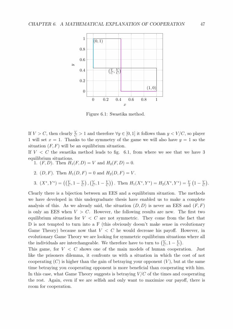
CHAPTER 6. A MATHEMATICAL EXPLANATION OF COOPERATION 47
0 0.2 0.4 0.6 0.8 1
0
0.2
0.4
0.6
0.8
1
(VC ,
VC
)
(0, 1)
(1, 0)
x
y
Figure 6.1: Swastika method.
If V > C, then clearly VC> 1 and therefore ∀y ∈ [0, 1] it follows than y < V/C, so player
1 will set x = 1. Thanks to the symmetry of the game we will also have y = 1 so thesituation (F, F ) will be an equilibrium situation.If V < C the swastika method leads to fig. 6.1, from where we see that we have 3equilibrium situations.
1. (F,D). Then H1(F,D) = V and H2(F,D) = 0.
2. (D,F ). Then H1(D,F ) = 0 and H2(D,F ) = V .
3. (X∗, Y ∗) =((
VC, 1− V
C
),(VC, 1− V
C
)). Then H1(X
∗, Y ∗) = H2(X∗, Y ∗) = V
2
(1− V
C
).
Clearly there is a bijection between an EES and a equilibrium situation. The methodswe have developed in this undergraduate thesis have enabled us to make a completeanalysis of this. As we already said, the situation (D,D) is never an EES and (F, F )
is only an EES when V > C. However, the following results are new. The first twoequilibrium situations for V < C are not symmetric. They come from the fact thatD is not tempted to turn into a F (this obviously doesn’t make sense in evolutionaryGame Theory) because now that V < C he would decrease his payoff. However, inevolutionary Game Theory we are looking for symmetric equilibrium situations where allthe individuals are interchangeable. We therefore have to turn to
(VC, 1− V
C
).
This game, for V < C shows one of the main models of human cooperation. Justlike the prisoners dilemma, it confronts us with a situation in which the cost of notcooperating (C) is higher than the gain of betraying your opponent (V ), but at the sametime betraying you cooperating opponent is more beneficial than cooperating with him.In this case, what Game Theory suggests is betraying V/C of the times and cooperatingthe rest. Again, even if we are selfish and only want to maximize our payoff, there isroom for cooperation.

CHAPTER 6. A MATHEMATICAL EXPLANATION OF COOPERATION 48
6.3 The Ultimatum Game
To conclude this chapter, it is convenient to analyze an experiment, the result of whichcannot be explained with the tools we have developed. Imagine that we randomly selecttwo people and we tell them to play the following game: Player 1 has to propose a wayto divide a certain quantity of money between the two players and then player 2 decidesif he accepts or rejects the deal. If he accepts, the distribution is carried out as player 1suggested, but if he rejects nobody gains anything. According to classical Game Theory,even if player 1 proposes to keep with 99% of the total amount and give only 1% toplayer 2, he should always accept the deal because something, even if it’s a paltry sum ofmoney, is better than nothing. The economist Ernst Fehr, from the University of Zurich,conducted this experiment to find that people do not adhere to the recommendations ofGame Theory. In fact, most of the times that player 1 offered player 2 less than 30%
of the initial value, the deal was rejected. When you reject a deal, you are sacrificing acertain economic gain in order to punish the other player. Those who renounce to a gaindo it for the greater good. The fact that you could increase your payoff is subordinatedto a bigger idea: you have to make sure your opponent does not increase his payoff. Thisconcept, known as altruistic punishment, is a crucial element in fostering cooperation. Atthe moment, nobody has been able to give an explanation for this in terms of self interest.This experiment, and other similar ones, has motivated the introduction of different kindsof players, apart form the selfish player, in Game Theory. This could be a good startto study Cooperative Game Theory. However, it is time for this undergraduate thesis tocome to an end.

Conclusions
In this undergraduate thesis the foundations of Noncooperative Game Theory have beenlaid. From a mathematical standpoint, Nash’s Theorem (Theorem (5.4)) represents thecornerstone of this senior thesis. It asserts that in any noncooperative game - regardlessof the number of players, of the number of strategies they can employ, etc - there is atleast one equilibrium situation. However, Nash’s Theorem falls under the category ofthose theorems which are only really appreciated by mathematicians. This is because,even if its implications are huge, it doesn’t give the slightest clue on how to find Nashequilibriums, i.e., it is not constructivist. Therefore, when it comes to applying GameTheory to real life, it is rather useless. The main goal of my senior thesis was to show howGame Theory could be used to tackle a great number of different problems. Throughoutthis undergraduate thesis, Game Theory has served us to design optimal war strategies,to study a duopoly or to analyze how animals contest a resource. However, from asocial standpoint, the cornerstone of this research work was to show that cooperativedispositions can indeed emerge in a world of selfish individuals.I would consider myself to be satisfied if I managed to convince the reader that GameTheory is a really useful tool to analyze all kinds of situations in which there is some sortof interaction. If I had the opportunity to pursue research in this field, I believe it wouldbe very interesting to study Cooperative Game Theory, as it would enable us to gain anew perspective and tackle a lot of new problems.
49
Bibliography
[1] N.N. Vorob’ev. Game Theory: Lectures for Economists and Systems Scientists. 1st.Ed. (Springer-Verlag. 1977)
[2] Julio González-Díaz, Ignacio García-Jurado and M. Gloria Fiestras-Janeiro. An In-troductory Course on Mathematical Game Theory. 1st. Ed. (Graduate Studies inMathematics. 2010)
[3] Saul Stahl. A Gentle Introduction to GAME THEORY. 1st Ed. (American Mathe-matical Society. 1999)
[4] Robert Axelrod. The Evolution of Cooperation. Revised edition. (Basic Books Inc.,Publishers. 1984)
[5] Fedorchuk V. General Topology I. 1st. Ed. (Springer-Verlag. 1990)
[6] Fudenberg D. and Tirole J. Game Theory. 1st Ed. (MIT Press. 1991)
[7] Aureli Alabert. Lecture notes from Introducció a la I.O. 2
[8] Cifre A. H. Lecture notes from Optimización Geométrica en Convexidad. Capítulo 1:Conjuntos convexos y sus propiedades. University of Murcia. (http://webs.um.es/mhcifre/apuntes/cap1.pdf)
[9] Ángel Sánchez. Las matemáticas de la cooperación humana (http://www.matematicalia.net/index.php?option=com_content&task=view&id=252&Itemid=169#ref16_txt).
[10] Hofbauer J. and Sigmund K. "Evolutionary Game Dynamics". Bulletin (New Series)of the American Mathematical Society. 40, 479–519 (2003).
[11] Stephen C. Stearns. Evolutionary Game Theory: Fighting and Contests. Open YaleCourses. (https://www.youtube.com/watch?v=aP25rlgwD54)
50