University of Central Florida University of Central Florida

STARS STARS

HIM 1990-2015

2015

Understanding and Modeling Pathways to Thrombosis Understanding and Modeling Pathways to Thrombosis

John Seligson University of Central Florida

Part of the Mechanical Engineering Commons

Find similar works at: https://stars.library.ucf.edu/honorstheses1990-2015

University of Central Florida Libraries http://library.ucf.edu

This Open Access is brought to you for free and open access by STARS. It has been accepted for inclusion in HIM

1990-2015 by an authorized administrator of STARS. For more information, please contact STARS@ucf.edu.

Recommended Citation Recommended Citation Seligson, John, "Understanding and Modeling Pathways to Thrombosis" (2015). HIM 1990-2015. 1743. https://stars.library.ucf.edu/honorstheses1990-2015/1743

UNDERSTANDING AND MODELING PATHWAYS TO THROMBOSIS

by

JOHN M. SELIGSON

A thesis submitted in partial fulfillment of the requirements

for the Honors in the Major Program in Mechanical Engineering

in the College of Engineering and Computer Science

and in the Burnett Honors College

at the University of Central Florida

Orlando, Florida

Spring Term 2015

Thesis Chair: Alain Kassab, Ph.D.

ii

ABSTRACT

Intra-vessel thrombosis leads to serious problems in patient health. Coagulation can

constrict blood flow and induce myocardial infarction or stroke. Hemodynamic factors in blood

flow promote and inhibit the coagulation cascade. Mechanically, high shear stress has been

shown to promote platelet activation while laminar flow maintains plasma layer separation of

platelets and endothelial cells, preventing coagulation. These relationships are studied

experimentally, however, physical properties of thrombi, such as density and viscosity, are

lacking in data, preventing a comprehensive simulation of thrombus interaction. This study

incorporates experimental findings from literature to compile a characteristic mechanical

property data set for use in thrombosis simulation. The focus of this study’s simulation explored

how thrombi interact between other thrombi and vessel walls via Volume of Fluid method. The

ability to predict thrombosis under specific hemodynamic conditions was also a feature of the

data collection. Using patient specific vessel geometry, the findings in this study can be applied

to simulate thrombosis scenarios. The possible applications of such a simulation include a more

precise method for estimation of patient myocardial infarction or stroke risk and a possible

analysis of vessel geometry modification under surgery.

iii

DEDICATION

To my sister,

for your love and support,

bringing joy and laughter to my world

iv

ACKNOWLEDGEMENTS

I would like to extend my gratitude to Dr. Alain Kassab for his mentorship and advice

throughout the process of this work. His knowledge, experience, and guidance improved my

educational experience and refined my abilities as a researcher.

To Dr. Faissal Moslehy and Dr. Eduardo Divo, thank you for overseeing my work and providing

helpful and constructive feedback. Your influence has been edifying and challenging, driving me

to excellence.

To my parents, David and Sherri Seligson, thank you for supporting me through my endeavors.

Specifically, thank you for cultivating me and providing a constructive environment in which to

grow, improving my confidence and instilling an excitement for learning and thinking deeply.

v

TABLE OF CONTENTS

LIST OF TABLES ........................................................................................................................ vii

LIST OF FIGURES ..................................................................................................................... viii

CHAPTER ONE: INTRODUCTION ............................................................................................. 1

CHAPTER TWO: THROMBUS FORMATION ........................................................................... 2

CHAPTER THREE: HEMODYNAMIC FACTORS PROMOTING THROMBOSIS ................. 5

CHAPTER FOUR: THROMBUS PROPERTIES .......................................................................... 8

Density ........................................................................................................................................ 8

Viscosity .................................................................................................................................... 11

Restitution ................................................................................................................................. 11

Shear to Break Free Vessel Wall Thrombi................................................................................ 12

Thrombus Properties Compilation ............................................................................................ 12

CHAPTER FIVE: THROMBOSIS MODEL ............................................................................... 14

Whole Blood properties ............................................................................................................ 14

Cardiovascular Induced Flow.................................................................................................... 16

Modeling method ...................................................................................................................... 16

Simulation ................................................................................................................................. 17

CHAPTER SIX: CONCLUSION ................................................................................................. 23

APPENDIX ................................................................................................................................... 24

vi

Appendix A: Non-Offset Thrombus to Thrombus Interaction................................................. 25

REFERENCES ............................................................................................................................. 26

vii

LIST OF TABLES

Table 1: White Thrombus Properties Compilation ....................................................................... 13

viii

LIST OF FIGURES

Figure 1: Summary of Blood Clotting Mechanisms (Lopez 294) .................................................. 4

Figure 2: Maximal Thrombin Concentration (Top), Time to Maximal Thrombin Concentration

(Middle), ETP (Bottom) vs. Hematocrit (Horne et al. 405) ............................................................ 6

Figure 3: Volume (Top), Mass (Middle), Density (Bottom) of Thrombi (Baker-Groberg, Phillips,

and McCarty 016014-3) ................................................................................................................ 10

Figure 4: Shear Stress vs. Shear Rate of Whole Blood (Christensen 35) ..................................... 15

Figure 5: Thrombus to Wall Collision Attempt ............................................................................ 18

Figure 6: Fast Thrombus to Wall Collision Attempt .................................................................... 19

Figure 7: Thrombus to Thrombus Collision ................................................................................. 20

Figure 8: Branching Geometry Thrombus Interaction (Part 1) .................................................... 21

Figure 9: Branching Geometry Thrombus Interaction (Part 2) .................................................... 21

Figure 10: Pressure Field of Branching Aorta .............................................................................. 22

Figure 11: Non-Offset Thrombus to Thrombus Interaction ......................................................... 25

1

CHAPTER ONE: INTRODUCTION

Thrombosis is a topic of much importance. As the circulatory system is vital for human

health, any blockage formed by a thrombus can cause major issues, including fatality. Modern

medicine sought to control coagulation via drugs such as warfarin. Such drugs present new

problems of gastrointestinal bleeding and intercerebral hemorrhage, due to the inhibition of

necessary coagulation (Kirklin et al. 18). In Kirklin’s and his colleagues’ studies, clot formation

was seen in the application of a left ventricular assist device (LVAD), where the inflow bearings,

inflow cannula, and outflow graft at spots of drastic change in direction were potential thrombus

sites (Kirklin et al. 18). Noticing the problem being caused by mechanical application, it follows

that a solution towards controlling thrombosis lies in understanding the mechanical aspects of

thrombus formation. This can be done by studying how thrombi form, the hemodynamic factors

that promote thrombosis, and thrombus mechanical properties. In understanding what a thrombus

is and what triggers it, a computer model can be made to simulate patient specific blood flow,

showing where, how, and when a thrombus would generate. Such a method would highly

influence the medical field and further equip medical specialists, giving patients facing

thrombotic issues a greater chance.

2

CHAPTER TWO: THROMBUS FORMATION

In order to stop blood loss in the event of vessel injury, the body must create a “plug.” When

a break in the vessel arises, platelets activate, adhering to collagen fibers in the damaged

endothelial cells, and produce pro-coagulant factors leading to the conversion of the plasma

protein, prothrombin, to the enzyme, thrombin. This enzyme also produces factors that create

more thrombin, which convert inactive fibrinogen present in blood to fibrin. Multiple fibrin lay

down to create a network or “mesh” in which red blood cells fill, creating a sufficient plug for

leakage prevention (Campbel 911-912). When these factors influence clot formation inside the

vessel instead of outside or in the vessel wall, the formed clot is considered a thrombus.

With a thrombus being formed in an intra-vascular location, the locations to analyze are

inside veins and arteries, from the vessel wall to the center of the blood flow. When platelets rest

and bind to proteins on the vessel wall causing platelet activation and adhesion, as well as

enzyme factor VIIa binding with receptors on endothelial cells, thrombin is formed. This

thrombin also causes platelet activation and fibrinolysis (Xu et al. 237). The first of these two

mechanisms, the activation of platelets, uses glycoproteins to bind to other platelets and

constituents. The second, fibrinolysis, recruits red blood cells to create a mesh, and contributes to

the structure of the clot (“Medical Physiology” 446B). The first mechanism mentioned is known

as white thrombus, while the second is known as red thrombus. On the vascular wall and in

blood are constituents which play roles in anti-thrombotic and pro-thrombotic states based on

when clots need to form (“Medical Physiology” 446C). For anti-thrombotic cases, endothelial

cells line the vascular wall and produce anticoagulant factors. If these cells are damaged or

removed due to injury, blood cells come into contact with pro-coagulant factors and thrombosis

3

occurs (“Medical Physiology” 446C). For pro-thrombotic cases, unusual shear can cause

platelets to activate. On top of this, according to Shadden, in areas of low velocity such as the

wall of the vein which also contain activated platelets lead to platelet adherence and coherence

(Shadden and Hendabadi 473).

Two pathways must be considered for thrombosis. The intrinsic pathway deals with blood

interacting with negatively charged surfaces or glass, followed by interaction with clotting factor

XII and other factors. The extrinsic pathway deals with blood interacting with damaged cells,

being exposed to tissue factor III, followed by interaction with clotting factor VII. Both of these

pathways cause procoagulent factors to “activate” which starts a chain of reactions towards a

common pathway terminating at formed thrombus (Medical Physiology 446E). To illustrate how

all of the factors orchestrate the formation of a thrombus, the following figure displays the

thrombosis cascade.

4

Figure 1: Summary of Blood Clotting Mechanisms (Lopez 294)

5

CHAPTER THREE: HEMODYNAMIC FACTORS PROMOTING

THROMBOSIS

There are several conditions in which the environment of vessel blood flow is pro-

thrombotic. A German physician, Rudolf Virchow, studied the subject of thrombosis

approximately one hundred fifty years ago. Though it was not proposed by him, a generalization

of hemodynamic factors were proposed and named after the physician, now known as Virchow’s

Triad (Bagot and Roopen 180). The three factors consist of the flow of blood in the vessel, the

type and amount of constituents in the blood, and injury to the endothelial wall (Kiyomura et al.

216). Regarding blood flow, abnormal fluid dynamic features such as turbulence and stasis

promote thrombosis. Normally, under laminar flow, a layer of plasma, moving slower than

regular blood flow, separates the constituents of blood from the endothelial wall. In the case of

non-laminar flow, the plasma layer can be ripped away, allowing platelets to touch the

endothelial wall and start pro-coagulant factors. Another unwanted situation, static blood flow

keeps coagulant factors in one location, preventing fresh, “inactivated” blood along with anti-

coagulant factors from diluting or replacing the pro-coagulant factors (Kiyomura et al. 216).

Concerning blood constituents, a high density of red blood cells can promote the formation of a

thrombus. An increase in hematocrit, or the volume percentage of red blood cells, can raise the

endogenous thrombin potential (ETP). Horne’s study provided that as hematocrit percentage rose

from 0% to 60%, the maximal thrombin concentration rose from zero to up to 78 nanomoles per

liter while the time to reach maximal thrombin concentration fell from 20 minutes to as low as

7.5 minutes. This data can be seen in Horne’s figure below.

6

Figure 2: Maximal Thrombin Concentration (Top), Time to Maximal Thrombin Concentration (Middle), ETP

(Bottom) vs. Hematocrit (Horne et al. 405)

The procedure was done by taking red blood cells from blood samples and sedimenting them

by centrifugation at 2000 g for 10 minutes. Lipidated tissue factor and CaCl2 was added to

promote clotting (Horne et al. 405). In support, Kiyomura’s study reported a value for hematocrit

above 51% poses risk for stroke (Kiyomura et al. 217). This suggests that at a certain red blood

cell density, a thrombus is more likely to form. Understanding that turbulence might cause an

7

increase in red blood cell density, a relationship between shear stress and hematocrit might exist.

This relation could be utilized in a computer model to show the formation of a thrombus. Finally,

in terms of endothelial injury, platelets can be activated when exposed to substances in damaged

endothelial cells such as collagen, resulting in adherence of the platelets to the damaged location

(Kiyomura et al. 217).

Another trigger for thrombosis can mechanically be represented as a function including high

shear stress for a period of time (Shadden and Hendabadi 467). In a study by Chesnutt, multiple

values of critical shear stress, the stress required to activate a platelet, were considered. Several

studies compiled by Chesnutt had resulted in critical shear stress values ranging from 2.3 – 32.0

N m-2 for whole blood and 1.5 – 12 N m-2 for platelet rich plasma. However, the study indicated

that, in vitro, high shear stress of 7.5 – 14 N m-2 as well as low shear stress of 1.5 – 3 N m-2 lead

to platelet activation (Chesnutt and Han 12). These two ranges could be used as the upper and

lower bounds for pro-thrombotic conditions, relating to high shear stress and stagnation in blood

flow. However, from the pathways stated above, it is obvious that thrombi do not form

instantaneously. To model such an action would sacrifice the reliability of the outcome. From the

same study, Chesnutt used a relationship for critical shear rate, the rate in which platelets are

activated. The relationship is such that �̇� = 𝜏𝜇𝑏⁄ , where �̇� is the critical shear rate (s-1), 𝜏 is the

critical shear stress (N m-2), and 𝜇𝑏 is the viscosity of the fluid, in this case, whole blood (kg m-1

s-1) (Chesnutt and Han 6). In the creation of a computer model as mentioned below, this equation

could be implemented using the range of critical shear stress to be 𝜏 = (1.5,3) ⋃(7.5,14) N m-2.

8

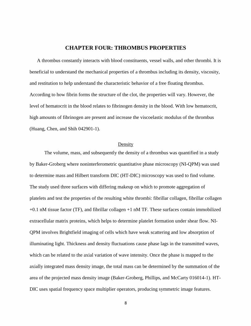
CHAPTER FOUR: THROMBUS PROPERTIES

A thrombus constantly interacts with blood constituents, vessel walls, and other thrombi. It is

beneficial to understand the mechanical properties of a thrombus including its density, viscosity,

and restitution to help understand the characteristic behavior of a free floating thrombus.

According to how fibrin forms the structure of the clot, the properties will vary. However, the

level of hematocrit in the blood relates to fibrinogen density in the blood. With low hematocrit,

high amounts of fibrinogen are present and increase the viscoelastic modulus of the thrombus

(Huang, Chen, and Shih 042901-1).

Density

The volume, mass, and subsequently the density of a thrombus was quantified in a study

by Baker-Groberg where noninterferometric quantitative phase microscopy (NI-QPM) was used

to determine mass and Hilbert transform DIC (HT-DIC) microscopy was used to find volume.

The study used three surfaces with differing makeup on which to promote aggregation of

platelets and test the properties of the resulting white thrombi: fibrillar collagen, fibrillar collagen

+0.1 nM tissue factor (TF), and fibrillar collagen +1 nM TF. These surfaces contain immobilized

extracellular matrix proteins, which helps to determine platelet formation under shear flow. NI-

QPM involves Brightfield imaging of cells which have weak scattering and low absorption of

illuminating light. Thickness and density fluctuations cause phase lags in the transmitted waves,

which can be related to the axial variation of wave intensity. Once the phase is mapped to the

axially integrated mass density image, the total mass can be determined by the summation of the

area of the projected mass density image (Baker-Groberg, Phillips, and McCarty 016014-1). HT-

DIC uses spatial frequency space multiplier operators, producing symmetric image features.

9

With the addition of low frequency components, edges of specimens in the DIC image cubes can

be detected. This HT-DIC method was determined to be valid for samples above 0.11 µm in

diameter (Baker-Groberg, Phillips, and McCarty 016014-2).

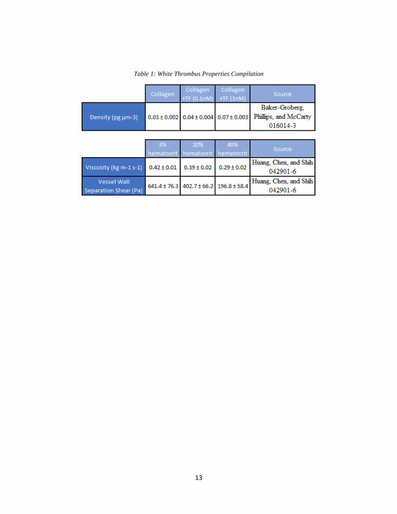
Using these two methods to find mass and volume of a sample of thrombi, a statistical

analysis was performed for the data Baker-Groberg collected and resulted in three average

values, with standard deviation, for thrombi: 0.03 ± 0.002 pg µm-3 for collagen, 0.04 ± 0.004 pg

µm-3 for collagen +TF (0.1nM), and 0.07 ± 0.003 pg µm-3 for collagen +TF (1nM) (Baker-

Groberg, Phillips, and McCarty 016014-3). The displayed data can be seen below.

10

Figure 3: Volume (Top), Mass (Middle), Density (Bottom) of Thrombi (Baker-Groberg, Phillips, and McCarty

016014-3)

Another study by Nahirnyak investigated the density of venous white thrombi by a

combination of fluid displacement method and laboratory scale. The method was conducted for

202 clots from 28 human participants and resulted in an average clot density of (1.08±0.02)x103

kg/m3 (Nahirnyak, Yoon, and Holland 3768, 3771). As thrombi are composed of several

different constituents in whole blood, the density of thrombi are more likely to share a similar

density to whole blood. This density is consistent with the density of whole blood as mentioned

11

later in this study. The data from Baker-Groberg was still used in the computer model to

understand how such a low density would affect the interaction of thrombi.

Viscosity

In a study done by Huang, the method of shear-wave dispersion ultrasound vibrometry

(SDUV) was used to analyze mechanical properties of thrombi. Tissue vibration induced shear

waves are caused by an ultrasound beam at a certain focal point. The shear wave propagation

speed in the tissue is then found by a second ultrasound transducer which detects shear wave

phase changes per distance. The results of the SDUV showed viscosity of the thrombus to be

0.42 ± 0.01 kg m-1 s-1 at 3% hematocrit, 0.39 ± 0.02 kg m-1 s-1 at 20% hematocrit, and 0.29 ±

0.02 kg m-1 s-1 at 40% hematocrit (Huang, Chen, and Shih 042901-6). Concerning input into a

computer model, the average human male and female has 45% and 40% hematocrit, respectively.

Though it depends on the patient for a patient specific model, the use of 0.29 kg m-1 s-1 for the

viscosity of a thrombus is reasonable for normal conditions.

Restitution

The thrombus to thrombus and thrombus to vessel wall interaction is important to

analyze, governing whether or not a thrombus will “stick” or “bounce off” in either interaction.

Due to the absence of experimental data to support the evaluation of thrombus restitution, this

study employed the use of a computational fluid dynamics (CFD) model using the two properties

listed above in a 2D flow field. A thrombus with an initial velocity at a specific angle of

incidence to the wall before collision will result in an opposite velocity after collision, relatable

to restitution. Observance of the computer simulation can provide a theoretical thrombus to wall

restitution coefficient. Another simulation involving multiple thrombi colliding can provide a

12

theoretical thrombus to thrombus restitution coefficient. The implementation of these simulations

can be seen in chapter five, however, the results were limited by the modeling method. The

modeled thrombi were simulated as fluid with densities and viscosities mentioned above. When

simulating a thrombus moving toward the vessel wall, the momentum of the drastically less

dense thrombus could not overcome the flow of whole blood. Therefore, a restitution coefficient

regarding thrombus to vessel wall could not be obtained. The nature of fluid modeling also made

each thrombus collide in a perfectly inelastic nature, only showing a restitution coefficient of 1.

In conclusion, modeling thrombi as fluid is not sufficient for restitution coefficients.

Shear to Break Free Vessel Wall Thrombi

It is important to understand the shear stress involved in breaking off a thrombus formed

on the wall of the vessel. In a computer model, the shear caused by blood flow may cause the

thrombus to shear off and enter the flow, resulting in downstream complications. In the same

study performed by Huang mentioned above, the use of SDUV resulted in the findings of the

shear modulus for a thrombus. The findings are as follows: 641.4 ± 76.3 Pa for 3% hematocrit,

402.7 ± 66.2 Pa for 20% hematocrit, and 196.8 ± 58.4 Pa for 40% hematocrit (Huang, Chen, and

Shih 042901-6). Using the same logic put forward in the viscosity report above, 196.8 Pa is

reasonable for use in the computer model.

Thrombus Properties Compilation

A collective table of hemodynamic properties of thrombi was made including the values

mentioned above. It should be noted that the studies that produced the properties focused on

white thrombi, formed by platelet activation. The collective properties used in this study’s

simulation can be used in future thrombus simulations.

13

Table 1: White Thrombus Properties Compilation

14

CHAPTER FIVE: THROMBOSIS MODEL

A computer model can be made, incorporating the physical properties of thrombus and

thrombosis triggers, to simulate the formation of a thrombus. As mentioned above, the critical

shear stress for platelet activation is assumed to be 𝜏 = (1.5,3) ⋃(7.5,14) N m-2. The

relationship �̇� = 𝜏𝜇𝑏⁄ can dictate the rate at which thrombi are formed. Berzi analyzes granular-

fluid mixtures with the “solids” being represented by spheres for simplicity (Berzi 547). Though

thrombi are not spherical, for simplification purposes, a sphere model is a good average shape

representation. The movement of the thrombus can be modeled, and when colliding with the

vessel wall with sufficient energy transfer, the model can simulate vessel wall damage, causing

thrombus spheres to form, stuck to the wall. Additionally, as mentioned above, negatively

charged surfaces trigger thrombosis. Based on the correct amount of shear in the fluid at a

specific location, the model can simulate the thrombus from both damaged and negatively

charged surfaces breaking off and joining the flow. For the purposes of this study, only thrombi

interaction was modeled to prove validity of thrombus properties and explore possible

characteristics of thrombi. A unique approach of modeling the thrombi as liquid with the given

properties includes the deformable nature of thrombi.

Whole Blood properties

In order to model thrombi as fluid interacting with whole blood, whole blood properties

must first be collected. The values for density and viscosity of whole blood were be utilized in

the model to generate realistic flow. A study performed by Trudnowski analyzed blood

contributed by six women and 19 men of good health and ages ranging from 29 to 58 years.

Taking the samples before lunch, 10 ml of whole blood was taken and separated into 2 ml

15

volumetric flasks. Weighing the samples at 4 oC and 37 oC, the relative density to water was

1.0621 for 4 oC and 1.0506 for 37 oC, both featuring a 95% confidence interval (Trudnowski,

Raymond, and Rico 615). This study incorporates 1050.6 kg/m3 as whole blood density for the

purposes of the thrombus simulation shown below. As for the average viscosity of whole blood,

Windberger’s study performed Haemorheology by LS30 viscometers for whole blood. The

viscometer was set at 0.7, 2.4, and 94 s-1 shear rates at 37 oC. Electromagnetic measurements of

mechanical strain by whole blood viscosity on the inner cylinder of the viscometer correlated to

the whole blood’s viscosity (Windberger et al. 432). The results of Windberger’s study gave

whole blood viscosity of 39.584 mPa s for 75th percentile (Windberger et al. 434). Blood at low

shear rates acts as a non-Newtonian fluid, as shown in the plot below.

Figure 4: Shear Stress vs. Shear Rate of Whole Blood (Christensen 35)

A Newtonian fluid acts exhibit a linear relationship for a plot of shear stress versus shear

rate. However, the red blood cells in whole blood cause a non-linear curve at low shear rates,

varying the viscosity with flow rate (Christensen 35). The whole blood viscosity from

Windberger’s study was reported at a low shear rate of 0.7 s-1. The viscosity decreased to 5.996

mPa s at a shear rate of 94 s-1 (Windberger et al. 434). Though 39.584 mPa s is large and only for

16

the non-Newtonian range, the value was still chosen for the simulation to observe how thrombi

would interact with such conditions.

Cardiovascular Induced Flow

In the model of blood flow, parameters need to be set to dictate the nature of the flow. In

other words, the amplitude and characteristic of pressure caused by the heart can be employed in

the model. For the purposes of relating this study’s findings to LVAD applications, the Aorta

was chosen as the blood vessel of interest. According to Lopez-Ojeda, systolic pressure of the

Aorta is 100mmHg, while the systolic velocity is approximately 0.11 m/s (Human Physiology

135).

Modeling method

Star CCM+ is a CFD program which employs several different methods regarding the

dynamic interaction of gasses, fluids, and solids. A fundamental method is known as the Volume

of Fluid (VoF) method. VoF is a numerical modeling method which is concerned with the

boundary layer between two fluids, and in this case, the thrombus is assumed to be a fluid with

the densities and viscosities mentioned above. Bo’s study describes the method well. VoF was

originally intended for incompressible fluids, but was later modified to compressible fluids. In

order to account for mixed phase flow, specific material particles with equilibrium of both

pressure and velocity and advecting specific entropies with the flow are seen as distanced from

each other by volume. More precisely, a computational cell consists of a volume fraction (a

mixture of different fluids) developed for half a time step, creating a reconstructed planar

interface at that cell. This is for constant thermodynamics. This reconstruction produces an

interface normal which positions the planar interface according to the separate fluid volumes.

17

The quantity of the individual fluid materials fluxing in the computational cells is then predicted

concerning the local flow velocity and the reconstructed interface. A second order Godunov

scheme is then used with the previously calculated quantities to improve the numerical fluxes.

Now, each computational cell has a single set of mass fluxes including the momentum and

energy fluxes. Thus, this result is intrinsically conservative (Bo and Grove 114).

According to Baraldi’s study, the VoF function, C, describes the volume fraction of the

reference phase between the two fluids where C = 0 refers to fluid one, C = 1 refers to fluid two,

and 0 ≤ C ≤ 1. VoF involves two steps: VoF interface reconstruction and VoF advection. The

interface reconstruction requires a piecewise linear interface calculation. To construct the

computational cell, the interface normal and the interface location must first be computed. VoF

advection involves the Eulerian implicit-Eulerian algebraic-Lagrangian explicit algorithm

(Baraldi, Dodd, and Ferrante, 324-325).

Simulation

Using the VoF code in Star CCM+ to model two phase liquid interaction, several

different flow scenarios were simulated. The first simulation attempted was to cause a collision

between a thrombus and the vessel wall. The geometry and fluid dynamic environment was

modeled as systolic conditions in the aorta. The height of the 2D tube was 3 cm.

18

Figure 5: Thrombus to Wall Collision Attempt

The volume fraction is shown as blue for whole blood and red for thrombus. The

simulated solution time was 0.13 seconds. The thrombus had an initial velocity at 45 degrees to

the horizontal. As seen in the figure above, the thrombus never reached the wall. Understanding

that the density of thrombi is much less than that of whole blood, the thrombus in this simulation

did not have enough momentum to overcome the whole blood flow. Another simulation was

performed with unrealistic initial velocity of the thrombus. This was done in order to force

collision with the wall.

19

Figure 6: Fast Thrombus to Wall Collision Attempt

The simulated solution time was 0.09 seconds. With an initial velocity of 2 m/s at a 45

degree angle from the horizontal, the thrombus is sheared by the whole blood flow and does not

collide with the wall. As indicated earlier in this study, restitution coefficients for thrombus to

wall interaction were unable to be quantified by the method of modeling thrombi as liquid. Next,

a simulation was run with two thrombi colliding in the flow.

20

Figure 7: Thrombus to Thrombus Collision

The simulated solution time was 0.84 seconds. The two thrombi collide at an offset and

show inelastic collision. The result of the offset collision made the combined thrombus drift

towards the bottom wall, however, the thrombus continued on the same path as the whole blood

flow and never collided with the wall. See the appendix for thrombus to thrombus collision with

no offset, a simulated solution time of 0.24 Seconds. The liquid thrombus modeling method

ensures inelastic collision due to the surface tension of the two fluids. However, this method can

be useful for early stage thrombosis as the physical property is a solid-fluid mixture. The final

simulation incorporated an arbitrary geometry of the aorta branching. This geometry was to

observe the interaction of multiple thrombi with the liquid thrombus modeling method.

21

Figure 8: Branching Geometry Thrombus Interaction (Part 1)

Figure 9: Branching Geometry Thrombus Interaction (Part 2)

22

The results from this simulation are noteworthy. As seen above, four thrombi of varying

sizes enter each branch. Concerning the pressure field as shown in figure 9, the larger thrombi

are effected more by pressure than the smaller thrombi. Figure 6 shows the thrombi in line in the

top branch, while the bottom branch has smaller thrombi overshooting the path of larger thrombi,

creating a collection of thrombi near the end of the branch. Figure 8 shows this collection

colliding and forming one large thrombus. This result suggests that the geometry of blood

vessels that create pressure variation along the cross-section can cause thrombus interaction and

larger thrombus formation. The irregularity of the cross-section geometry of the bottom branch is

what causes this pressure variation.

Figure 10: Pressure Field of Branching Aorta

23

CHAPTER SIX: CONCLUSION

With the application of predicting myocardial infarction or stroke, the findings of this

study are of great significance. The Volume of Fluid method utilized by the Star CCM+ model

provided a unique method to characterize thrombus interaction to vessel walls and other thrombi.

Physical properties of thrombi, including density and viscosity, collected by this study allow for

accurate simulation of thrombus interaction in patient specific vessel geometry applications.

Quantified hemodynamic factors for thrombosis also give way to accurate simulation of sites for

thrombosis in blood flow fields. Understanding the experimental relationships of thrombosis and

quantifying these relationships contribute to a proper method of thrombus analysis and

subsequent treatment, reducing possible risk of serious health problems in patients.

24

APPENDIX

25

Appendix A: Non-Offset Thrombus to Thrombus Interaction

Figure 11: Non-Offset Thrombus to Thrombus Interaction

26

REFERENCES

Bagot, Catherine N., Roopen Arya. “Virchow and his triad: a question of attribution.” British

Journal of Haematology 143. (2008): 180-190. Print.

Baker-Groberg, Sandra M., Kevin G. Phillips, and Owen J. T. McCarty. “Quantification of

volume, mass, and density of thrombus formation using brightfield and differential

interference contrast microscopy.” Journal of Biomedical Optics 18(1). (2013): 016014-1

- 016014-4. Print.

Baraldi, A., M.S. Dodd, and A. Ferrante. “A mass-conserving volume-of-fluid method: Volume

tracking and droplet surface-tension in incompressible isotropic turbulence.” Computers &

Fluids 96. (2014): 322-337. Print.

Berzi, D. “Simple Shear Flow of Collisional Granular-Fluid Mixtures.” J. Hydraul. Eng. 139.

(2013): 547-549. Print.

Bo, Wurigen, John W. Grove. “A volume of fluid method based ghost fluid method for

compressible multi-fluid flows.” Computers & Fluids 90. 113-122. Print.

Campbell, Neil A. et al. Biology. San Francisco: Pearson Education, Inc., 2011. Print.

Chesnutt, Jennifer K. W., and Hai-Chao Han. “Platelet size and density affect shear-induced

thrombus formation in tortuous arterioles.” Physical Biology 10. (2013): 16pp. Print.

27

Christensen, Douglas A., Introduction to Biomedical Engineering: Biomechanics and

Bioelectricity. Morgan & Claypool Publishers. 2009. Print.

Horne, McDonald K III, Ann M. Cullinane, Paula K. Merryman, and Elizabeth K. Hoddeson.

“The effect of red blood cells on thrombin generation.” British Journal of Haematology

133. (2006): 403–408. Print.

Huang, Chih-Chung, Pay-Yu Chen, and Cho-Chiang Shih. “Estimating the viscoelastic modulus

of a thrombus using an ultrasonic shear wave approach.” Medical Physics 40.4 (2013):

042901-1–042901-7. Print.

Kirklin, James K. et al. “Interagency Registry for Mechanically Assisted Circulatory Support

(INTERMACS) analysis of pump thrombosis in the HeartMate II left ventricular assist

device.” J Heart Lung Transplant 33. (2014): 12-22. Print.

Kiyomura, Masaki, Tomihiro Katayama, Yasuki Kusanagi, and Masaharu Ito. “Ranking the

contributing risk factors in venous thrombosis in terms of therapeutic potential:

Virchow’s triad revisited.” J. Obstet. Gynaecol. Res. 32.2 (2006): 216-223. Print.

Liu, W., C. R. Carlisle, E. A. Sparks, and M. Guthold. “The mechanical properties of single

fibrin fibers.” Journal of Thrombosis and Haemostasis 8. (2010): 1030–1036. Print.

Lopez-Ojeda, Wilfredo. Integrated Human Physiology: Laboratory Book and Manual.

Michigan: Hayden-McNeil Publishing. 2015. Print.

Medical Physiology. Atlanta: Elsevier, 2006. Print.

28

Nahirnyak, Volodymyr M., Suk Wang Yoon, and Christy K. Holland. “Acousto-mechanical and

thermal properties of clotted blood.” Journal of the Acoustical Society of America 119(6).

(2006): 3766-3772. Print.

Shadden, Shawn C., and Sahar Hendabadi. “Potential fluid mechanic pathways of platelet

activation.” Biomech Model Mechanobiol 12. (2013): 467–474. Print.

Trudnowski, Raymond J., Rodolfo C. Rico. “Specific Gravity of Blood and Plasma at 4 and 37

oC.” Clin. Chem. 20. (1974): 615-616. Print

Weisel, J. W. “Biomechanics in hemostasis and thrombosis.” Journal of Thrombosis and

Haemostasis 8. (2010): 1027–1029. Print.

Windberger, U., A. Bartholovitsch, R. Plasenzotti, K. J. Korak. “Whole blood viscosity, plasma

viscosity and erythrocyte aggregation in nine mammalian species: reference values and

comparison of data.” Experimental Physiology 88.3. (2003): 432, 434. Print.

Xu, Zhiliang, Oleg Kim, Malgorzata Kamocka, Elliot D. Rosen, and Mark Alber. “Multiscale

models of thrombogenesis.” WIREs Syst Biol Med 4. (2012): 237–246. Print.

Yamaguchi, Takami et al. “Particle-Based Methods for Multiscale Modeling of Blood Flow in

the Circulation and in Devices: Challenges and Future Directions.” Annals of Biomedical

Engineering 38.3 (2010): 1225–1235. Print.