Understanding Asymmetric Links, Buffers and

Bi-Directional TCP Performance

by

Sears Merritt

B.S., University of Colorado, 2004

A thesis submitted to the

Faculty of the Graduate School of the

University of Colorado in partial fulfillment

of the requirements for the degree of

Master of Science

Department of Interdisciplinary Telecommunications

2010

UMI Number: 1481150

All rights reserved

INFORMATION TO ALL USERS The quality of this reproduction is dependent upon the quality of the copy submitted.

In the unlikely event that the author did not send a complete manuscript

and there are missing pages, these will be noted. Also, if material had to be removed, a note will indicate the deletion.

UMI 1481150

Copyright 2010 by ProQuest LLC. All rights reserved. This edition of the work is protected against

unauthorized copying under Title 17, United States Code.

ProQuest LLC 789 East Eisenhower Parkway

P.O. Box 1346 Ann Arbor, MI 48106-1346

This thesis entitled:Understanding Asymmetric Links, Buffers and Bi-Directional TCP Performance

written by Sears Merritthas been approved for the Department of Interdisciplinary Telecommunications

Timothy X Brown

Doug Sicker

Kenneth Baker

Date

The final copy of this thesis has been examined by the signatories, and we find that both thecontent and the form meet acceptable presentation standards of scholarly work in the above

mentioned discipline.

iii

Merritt, Sears (M.S., Telecommunications)

Understanding Asymmetric Links, Buffers and Bi-Directional TCP Performance

Thesis directed by Professor Timothy X Brown

Asymmetric uplink and downlink rates are common in many broadband access networks,

particularly DSL, DOCSIS, and cellular. With the advent of peer-to-peer protocols and pervasive

devices supporting multimedia capabilities, bi-directional TCP traffic has also become commonplace

[1]. Under conditions where TCP connections are sending data in both directions simultaneously,

performance, as we will show, can be severely degraded.

This thesis seeks to determine how buffers, combined with elementary queueing strategies

like FIFO, influence bi-directional TCP performance across asymmetric network links. It also seeks

to determine if there is a way to size buffers such that the throughput for a small number of

bi-directional connections is optimized.

To answer this question, fundamental system components and algorithms will be reviewed.

Following this, research pertaining to observations, optimization techniques and design spaces will

be analyzed. Next, a set of real world experiments will be analyzed. Finally, a buffer sizing model

will be proposed that optimizes throughput for the bi-directional, long lived, TCP traffic under a

FIFO queueing strategy.

Practically speaking, this thesis seeks to determine if current consumer grade customer

premise equipment is designed to provide adequate performance for bi-directional Internet traf-

fic across typical asymmetric access technologies like DSL and DOCSIS.

iv

Acknowledgements

I would like to acknowledge and deeply thank Dr. Timothy X Brown and Dr. Martin Huesse

for their technical expertise in the field of networking and guidance in conducting professional

research. Without their continuous input and feedback this work would most certainly have not

been possible.

v

Contents

Chapter

1 Introduction 1

1.1 Contestability and Significance . . . . . . . . . . . . . . . . . . . . . . . . . . . . . . 5

1.2 Scope . . . . . . . . . . . . . . . . . . . . . . . . . . . . . . . . . . . . . . . . . . . . 6

1.3 Approach . . . . . . . . . . . . . . . . . . . . . . . . . . . . . . . . . . . . . . . . . . 7

2 Background and Prior Work 8

2.1 TCP . . . . . . . . . . . . . . . . . . . . . . . . . . . . . . . . . . . . . . . . . . . . . 8

2.2 TCP Phenomena and Performance Impacts . . . . . . . . . . . . . . . . . . . . . . . 10

2.3 Buffers . . . . . . . . . . . . . . . . . . . . . . . . . . . . . . . . . . . . . . . . . . . . 12

2.3.1 Architectures . . . . . . . . . . . . . . . . . . . . . . . . . . . . . . . . . . . . 12

2.3.2 Components . . . . . . . . . . . . . . . . . . . . . . . . . . . . . . . . . . . . 13

2.3.3 Sizing . . . . . . . . . . . . . . . . . . . . . . . . . . . . . . . . . . . . . . . . 13

2.4 Queueing Strategies . . . . . . . . . . . . . . . . . . . . . . . . . . . . . . . . . . . . 14

2.5 Drop Strategies . . . . . . . . . . . . . . . . . . . . . . . . . . . . . . . . . . . . . . . 15

2.6 Prior Work . . . . . . . . . . . . . . . . . . . . . . . . . . . . . . . . . . . . . . . . . 16

3 System Dynamics 25

3.1 Round Trip Time . . . . . . . . . . . . . . . . . . . . . . . . . . . . . . . . . . . . . . 26

3.2 Windows . . . . . . . . . . . . . . . . . . . . . . . . . . . . . . . . . . . . . . . . . . 26

3.3 Asymmetry . . . . . . . . . . . . . . . . . . . . . . . . . . . . . . . . . . . . . . . . . 26

vi

3.4 Buffering . . . . . . . . . . . . . . . . . . . . . . . . . . . . . . . . . . . . . . . . . . 27

3.5 Challenge of Asymmetric Links . . . . . . . . . . . . . . . . . . . . . . . . . . . . . . 27

4 Experiments 30

4.1 Introduction . . . . . . . . . . . . . . . . . . . . . . . . . . . . . . . . . . . . . . . . . 30

4.2 Network and Host Equipment . . . . . . . . . . . . . . . . . . . . . . . . . . . . . . . 31

4.3 Router Buffer and Queueing Configuration . . . . . . . . . . . . . . . . . . . . . . . 31

4.4 TCP Configuration . . . . . . . . . . . . . . . . . . . . . . . . . . . . . . . . . . . . . 32

4.5 Software . . . . . . . . . . . . . . . . . . . . . . . . . . . . . . . . . . . . . . . . . . . 32

4.6 Time Synchronization . . . . . . . . . . . . . . . . . . . . . . . . . . . . . . . . . . . 33

4.7 Post Processing . . . . . . . . . . . . . . . . . . . . . . . . . . . . . . . . . . . . . . . 33

4.7.1 Averages and Ratios . . . . . . . . . . . . . . . . . . . . . . . . . . . . . . . . 34

4.7.2 Tcpdump, Wireshark, Mergecap . . . . . . . . . . . . . . . . . . . . . . . . . 34

4.7.3 Gnuplot . . . . . . . . . . . . . . . . . . . . . . . . . . . . . . . . . . . . . . . 35

5 Results 36

5.1 Observations . . . . . . . . . . . . . . . . . . . . . . . . . . . . . . . . . . . . . . . . 36

5.1.1 Connection Synchronization . . . . . . . . . . . . . . . . . . . . . . . . . . . . 36

5.1.2 ACK Compression . . . . . . . . . . . . . . . . . . . . . . . . . . . . . . . . . 42

5.1.3 Random and Periodic Connection Interference . . . . . . . . . . . . . . . . . 42

5.1.4 BDP Tracking . . . . . . . . . . . . . . . . . . . . . . . . . . . . . . . . . . . 43

5.1.5 Summary . . . . . . . . . . . . . . . . . . . . . . . . . . . . . . . . . . . . . . 44

6 Optimization 46

6.1 Introduction . . . . . . . . . . . . . . . . . . . . . . . . . . . . . . . . . . . . . . . . . 46

6.2 Review of System Dynamics . . . . . . . . . . . . . . . . . . . . . . . . . . . . . . . . 46

6.3 Uplink Buffer Sizing Model . . . . . . . . . . . . . . . . . . . . . . . . . . . . . . . . 48

6.4 Use Case and Procedure . . . . . . . . . . . . . . . . . . . . . . . . . . . . . . . . . . 51

vii

6.5 Summary . . . . . . . . . . . . . . . . . . . . . . . . . . . . . . . . . . . . . . . . . . 53

7 Conclusions 55

Bibliography 56

Appendix

A Router Shaper Configuration 59

B TCP Server 61

C TCP Client 63

D Bandwidth Delay Product Estimation Script 66

E Download Averaging Script 67

F Upload Averaging Script 69

G Maximum CWND Script 70

H Buffer Estimation Script 71

I Performance Script 72

J RTT Variability Script 73

viii

Tables

Table

2.1 TCP State Variables . . . . . . . . . . . . . . . . . . . . . . . . . . . . . . . . . . . . 8

2.2 Prior Work Summary . . . . . . . . . . . . . . . . . . . . . . . . . . . . . . . . . . . 24

4.1 Experiment Configuration . . . . . . . . . . . . . . . . . . . . . . . . . . . . . . . . . 30

4.2 Equipment Setup . . . . . . . . . . . . . . . . . . . . . . . . . . . . . . . . . . . . . . 31

4.3 Traffic Shaper Configuration . . . . . . . . . . . . . . . . . . . . . . . . . . . . . . . . 31

4.4 TCP Options . . . . . . . . . . . . . . . . . . . . . . . . . . . . . . . . . . . . . . . . 32

4.5 Collected TCP Variables . . . . . . . . . . . . . . . . . . . . . . . . . . . . . . . . . . 32

5.1 Uplink Packet Buffer in Packets and Seconds . . . . . . . . . . . . . . . . . . . . . . 43

6.1 Average RTT . . . . . . . . . . . . . . . . . . . . . . . . . . . . . . . . . . . . . . . . 49

6.2 Results Summary . . . . . . . . . . . . . . . . . . . . . . . . . . . . . . . . . . . . . . 51

ix

Figures

Figure

1.1 Throughput with 50 and 15 Packet Uplink Buffers for 2.4Mbps Downlink and 196Kbps

Uplink . . . . . . . . . . . . . . . . . . . . . . . . . . . . . . . . . . . . . . . . . . . . 3

3.1 Test Network . . . . . . . . . . . . . . . . . . . . . . . . . . . . . . . . . . . . . . . . 25

3.2 Sequence of Events . . . . . . . . . . . . . . . . . . . . . . . . . . . . . . . . . . . . . 28

5.1 Performance for Asymmetric Link Combinations of 3, 12, 30 . . . . . . . . . . . . . . 37

5.2 Throughput with 5 Packet Uplink Buffer for 2.4Mbps Downlink and 196Kbps Uplink 37

5.3 Throughput with 20 Packet Uplink Buffer for 2.4Mbps Downlink and 196Kbps Uplink 37

5.4 Throughput with 25 Packet Uplink Buffer for 2.4Mbps Downlink and 196Kbps Uplink 38

5.5 Throughput with 50 Packet Uplink Buffer for 2.4Mbps Downlink and 196Kbps Uplink 38

5.6 10 Packet Uplink Buffer - Out of Phase CWND for 2.4Mbps Downlink and 196Kbps

Uplink . . . . . . . . . . . . . . . . . . . . . . . . . . . . . . . . . . . . . . . . . . . . 38

5.7 50 Packet Uplink Buffer - In Phase CWND for 2.4Mbps Downlink and 196Kbps Uplink 39

5.8 50 Packet Uplink Buffer for 2.4Mbps Downlink and 196Kbps Uplink . . . . . . . . . 39

5.9 5 Packet Uplink Buffer for 2.4Mbps Downlink and 196Kbps Uplink . . . . . . . . . . 40

5.10 20 Packet Uplink Buffer for 2.4Mbps Downlink and 196Kbps Uplink . . . . . . . . . 40

5.11 25 Packet Uplink Buffer for 2.4Mbps Downlink and 196Kbps Uplink . . . . . . . . . 41

5.12 Uplink Buffer vs. RTT Variability . . . . . . . . . . . . . . . . . . . . . . . . . . . . 45

6.1 Test Network RTT Components . . . . . . . . . . . . . . . . . . . . . . . . . . . . . . 47

x

6.2 Actual Buffer vs. Estimated Buffer for Asymmetric Link Combinations . . . . . . . 50

6.3 Real World Network with Asymmetric Link Ratio of X / Y . . . . . . . . . . . . . . 51

Chapter 1

Introduction

Asymmetric uplink and downlink rates are common in many broadband access networks,

particularly ADSL, DOCSIS, and cellular. With the advent of peer-to-peer protocols and pervasive

devices supporting multimedia capabilities, bi-directional TCP traffic has also become commonplace

[1]. Under conditions where TCP connections are sending data in both directions simultaneously,

performance, as we will show, can be severely degraded, in some cases as low as 20%.

This thesis presents an analysis of how packet-based buffers, combined with FIFO queueing,

affect bi-directional TCP performance across asymmetric network links. We also go on to present a

buffer sizing strategy for these links that provides performance of at least 68% across three different

combinations of asymmetric links.

As we will show, the main interaction between bi-directional traffic and buffer size is round

trip time (RTT) variability. In TCP, RTT is the cumulative time required to send data and receive a

corresponding acknowledgement. This time includes propagation delay, insertion time, processing,

and during periods of congestion, queueing delay in buffers. Improperly sized buffers can lead to

large amounts of RTT variability, which in turn inhibits the TCP sender’s ability to effectively size

its CWND to the bandwidth delay product (BDP) of the path. As we will show, these problems

occur when buffers are sized too large. Our sizing strategy provides a way to estimate a maximum

buffer size such that RTT variability is limited, thus allowing TCP sender’s to accurately track the

2

BDP of the path over the lifetime of the connection.

To illustrate the scenario of bi-directional TCP traffic across an asymmetric link with poorly

sized buffers, consider the following scenario: A user is streaming a video from Hulu across a typical

DSL link. In the middle of the video, the user decides to upload a personal movie clip to Facebook.

During the period where the movie clip is uploaded, the quality of the Hulu video is degraded to

the point where it is not viewable. We determine why this occurs and then go on propose a method

for avoiding it.

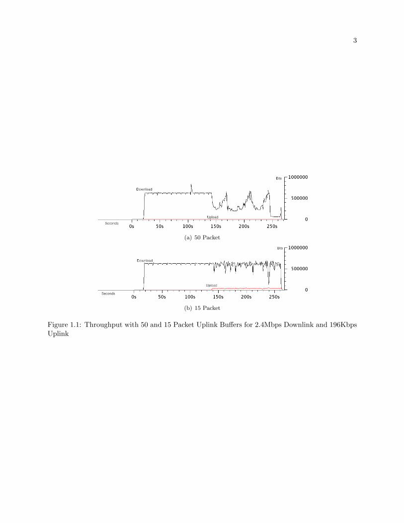
To begin to understand why this phenomenon occurs, we also present this scenario through

a graphical representation. In Figure 1.1(a) we show throughput over time for two connections, a

download in black and an upload in red. In this system, the uplink and downlink buffers are 50

packets. The upload is launched around time 150. Once the upload is present in the system, the

download throughput is degraded by about 50%. We contrast this performance with Figure 1.1(b).

Here we show the same scenario, but this time with the uplink buffer sized using our proposed model.

When the upload is started around time 150s, the download performance is hardly changed. In

this scenario the download throughput does not vary as widely as in Figure 1.1(a). It is clear that

uplink buffer size plays a dominant role in determining performance for two-way TCP traffic.

Through these examples, it is clear that this problem has real significance in networks. To

understand why this problem occurs, we first characterize the system by defining a set of terms

and metrics. We will then then go on to analyze the dynamics, present our buffer sizing strategy,

and measure its effectiveness.

Asymmetry occurs in a network when the link rates in each direction of a path are not equal.

This asymmetry can take on many forms. We highlight a set of three different configurations as

examples. First, a link can be asymmetric if the amount of physical bandwidth allocated to each

direction on the link is unequal. This type of configuration is common in access networks served

by xDSL technology. In ADSL, links to each subscriber are provisioned with asymmetric levels

3

(a) 50 Packet

(b) 15 Packet

Figure 1.1: Throughput with 50 and 15 Packet Uplink Buffers for 2.4Mbps Downlink and 196KbpsUplink

4

of bandwidth in the downstream and upstream directions. It is common for downstream links to

be provisioned with more bandwidth than the upstream. This bandwidth provisioning scheme is

deployed to align with a common traffic pattern where large quantities of data are downloaded

and small quantities are uploaded. Next, asymmetry can occur across links that are shared. In

shared medium, access to the channel is typically controlled by an access control protocol whereby

each subscriber is allocated a portion of the total link bandwidth in either direction. Again, it is

typical for access to the channel to be asymmetric for the reasons mentioned previously. Examples

of this type of link are found in wireless technologies like IEEE 802.16 or DOCSIS. Finally, it is

also possible to encounter an asymmetric link where routing protocols or other traffic engineering

technologies have selected paths or rate controlled the traffic in downstream and upstream directions

such that they operate at different rates. Often times, routing protocols like BGP or OSPF and

traffic engineering techniques like MPLS-TE are used to implement these types of paths. It is

important to understand in this final example that the asymmetry does not occur because of an

asymmetric physical link. It occurs because either the rates allocated to the forward and reverse

paths, which can consist of many links, are different.

The level of asymmetry is expressed as a ratio of the downlink and uplink bit rates,

Asymmetry Ratio = CD/CU , (1.1)

where CD is the capacity of the downlink and CU is the capacity of the uplink. It is typical that

the downlink operates at a higher rate than the uplink.

Two way, or bi-directional TCP traffic is comprised of two TCP connections sending data

in opposite directions. The TCP senders are on opposite sides of the asymmetric link operating

over separate sockets. In practice, two distinct pairs of hosts could terminate the TCP traffic in

each direction. In the experiments conducted in this research, two individual hosts were used to

originate and terminate the two way TCP traffic.

5

We use the minimum of the normalized goodputs of the TCP connections sending data

across the asymmetric link to measure the performance of the system and our buffer sizing model.

As we will show later, by changing the size of the uplink buffer, it is possible to manipulate

the performance of the system. We choose this metric because it provides fairness to both TCP

connections, as compared to other metrics, such as normalized net goodput, that favors one link

more than the other based on the level of asymmetry between the downlink and uplink. In (1.2)

let GD and GU equal goodput for the download and upload respectively. Let CD and CU equal

capacity of the downlink and uplink.

Performance = min(GU/CU , GD/CD) (1.2)

Using data collected from the experiments we estimate a maximum buffer size. As we will go on to

show in more detail, this estimation model is derived from work by Zhang et al. in [2]. To verify

our model’s accuracy, we compare the performance realized near the estimated buffer size to the

performance of all other measurements in the link configuration set. In all cases, the buffer size

estimated through our model yields values for all tested asymmetric link configurations of at least

68%, whereas any larger measured buffer size yields a further decrease of at least 10% and in some

cases up to 30%.

1.1 Contestability and Significance

The problem of maximizing performance of bi-directional TCP traffic across asymmetric

links still remains widely unsolved [3] [4]. Researchers have taken many different approaches to

solving the issue. Some have chosen to focus on end-to-end solutions while others propose localized

solutions that are implemented on intermediate nodes. In each of these approaches, researchers

use many different methodologies ranging from queueing, to new TCP variants. In any case, a well

agreed upon strategy to solve this problem still remains at large.

6

Regardless of the approach taken, the problem is well known throughout industry. RFC 3449

details performance problems experienced across asymmetric links. It presents strategies for both

localized and end-to-end solutions. That is, strategies that can be implemented at intermediate

nodes as well as at the hosts. In intermediate nodes, the authors recommend queueing techniques

such as random early detection (RED) and acknowledgement segment (ACK) prioritization. At

end hosts, sender pacing, compression and window prediction are recommended methodologies to

improve TCP performance across an asymmetric link [5].

1.2 Scope

This thesis is written for network designers, researchers and software engineers with sufficient

knowledge of basic network concepts including packet switching, the layering or encapsulation

model, the TCP/IP protocol suite [6], and basic queueing theory concepts. As we will show later,

our experiments focus on TCP/IPv4 traffic, however our solution is independent of the network

layer protocol and can support any packet based, connectionless network protocol encapsulating

TCP segments. This includes IPv6.

We aim to solve the problem of poor bi-directional TCP performance across asymmetric

links by limiting the solution to one that is localized. We further focus our solution towards access

networks where asymmetric access links are common, and, as we will show in reviewing prior work,

where the majority of potential delay in a network is stored.

Within the localized solution set, we choose to focus on buffering and FIFO queueing versus

TCP proxy or a complex queueing strategy for two main reasons. First, choose this strategy because

we assume that typical CPE nodes can easily support simple FIFO queueing and adjusting buffers,

whereas the other two solutions may be more difficult to implement on current platforms for both

technical and economical reasons. We base this assumption on specifications and pricing for typical

CPE nodes listed in [7] and [8]. We also argue that because the slow uplink is close to the affected

7

TCP endpoint, the user will be motivated to resolve this problem; as opposed to the slow uplink

being located in the network core and far away from any of the affected users.

We choose a localized approach versus an end-to-end approach because the problem is isolated

to asymmetric links and two-way TCP traffic. Because of this and the fact that most end devices

running TCP are now mobile and attach to many different types of networks, changing TCP to

address this specific problem at the possible expensive of introducing new ones does not make

sense.

1.3 Approach

We first analyze the existing literature in detail and develop a simple buffer sizing strategy

in Chapter 2. In Chapter 3 we go on to discuss the TCP system dynamics with and without our

strategy. To test our strategy we take an empirical approach and conduct a set of experiments on

a test network containing two hosts that send data to each other across an asymmetric link. The

experiments are organized as follows: We define a set of asymmetric links with asymmetry values

of 30, 12, and 3. For each asymmetry configuration, we vary uplink buffer size from 5 packets up

to the size of the downlink buffer, which is 50 packets, in increments of 5 packets. For each of the

buffer configurations we first launch a download and allow it to run without the presence of an

upload for 2 minutes. After the 2 minutes, we launch an upload and allow both the download and

upload to run across the network for an additional 2 minutes. Throughout the life of each of the

connections, we gather TCP state information using software that we have developed and describe

in Chapter 4. This TCP state information is then used to estimate maximum uplink buffer size

via our buffer sizing model. We then go on to verify its effectiveness at maintaining a high level of

performance compared to all other measured buffer sizes. These results are described in Chapters

5 and 6. We draw conclusions and describe future work in Chapter 7.

Chapter 2

Background and Prior Work

2.1 TCP

TCP is the de-facto standard for reliably transmitting information over IP based networks.

The protocol can be classified as a reliable byte-stream based on the concept of a sliding window.

The designers created TCP such that it utilizes the maximum available bandwidth in a system,

while at the same time sharing it with others. It is assumed that the underlying network is reliable

and yields low levels of packet loss. Based on this assumption, any packet loss experienced by TCP

is assumed to be due to congestion somewhere along the path between the sender and receiver. To

avoid congestion, it also employs adaptive algorithms to control the rate at which information is

injected into the network [9].

Three Way Handshake: At the genesis of a TCP connection, the sender and receiver perform

a three way handshake to open the connection and negotiate transmission options. The initiator

of the connection sends a SYN segment to the receiver. The receiver then responds to the SYN

with a SYN-ACK. The initiator follows this with an ACK. During this phase of a TCP connec-

tion initial window size, options like maximum segment size (MSS), window scaling, and selective

Table 2.1: TCP State Variables

TCP VariablesRTT SSTHRESH CWND

9

acknowledgement are negotiated [9].

Slow Start: Slow start is performed following the genesis of a connection. During this phase of the

connection, the sender begins transmitting data such that after each received ACK segment, the

window is increased by one MSS. This type of increase leads to exponential growth of the sender

window [10].

Congestion Avoidance: The congestion avoidance phase of TCP occurs once the CWND has

grown larger than the so-called slow start threshold, (SSTHRESH). In this phase TCP is trying to

utilize any additional bandwidth available on the link while at the same time avoiding packet loss.

Window growth in this phase is controlled via the additive increase algorithm. That is, after every

round trip time (RTT), the CWND is increased by one MSS [10].

Fast Retransmission: Fast retransmission is an algorithm to reduce the time it takes TCP to

recover from a lost segment. Upon detection of a lost segment by receiving 3 duplicate ACKs, TCP

immediately sends the lost segment without waiting for the retransmission timeout (RTO) value

to expire [10].

Fast Recovery: Following fast retransmission of the lost segment, TCP remains in congestion

avoidance phase and sets SSTHRESH to 1/2 of CWND. Next, CWND is set equal to SSTHRESH

+ 3·MSS. For each duplicate ACK received, the CWND is incremented by a MSS. If allowed, new

data is sent into the network. Finally, when the ACK for the first lost segment is received, CWND

is set equal to SSTHRESH [10].

Bandwidth Delay Product: The slow start and congestion avoidance algorithms in TCP are

used to accurately identify and track the bandwidth delay product (BDP) of a network path. The

BDP can be defined as the number of bytes in transit. The TCP sender window should track this

10

value to keep the utilization of the link maximized:

BDP = C ·RTT/8, (2.1)

where C is the bottleneck link speed in bits per second and RTT is the round trip time in seconds.

TCP depends on a steady BDP in order to utilize the link efficiently. In TCP, the congestion

avoidance algorithm cannot tolerate large amounts of variability in this value because it only adjusts

its window by a single MSS per RTT. As we will go on to show, when large amounts of variable delay

are introduced into the network, TCP connections in congestion avoidance mode cannot accurately

track the BDP of the link. This poor tracking leads to poor performance. We will carefully examine

how buffer size effects BDP tracking and go on to recommend a methodology for sizing buffers such

that a TCP can track the BDP accurately.

Selective Acknowledgement: Selective acknowledgement (SACK) allows the receiver to inform

the sender that certain amounts of discontiguous data have been received. When the receiver

acknowledges discontiguous data it does not advance the window via an ACK. Rather, it simply

acknowledges the blocks of data within the current window that have been received by sending a

SACK segment. This allows the sender to retransmit only the lost segments and not any duplicate

data.

2.2 TCP Phenomena and Performance Impacts

TCP can experience performance problems that result in degraded goodput when fundamen-

tal assumptions of its algorithm break down. These include stable RTT, timely arrivals of ACK

segments, low packet loss, and constant bandwidth.

ACK Compression: ACK compression is a phenomena observed when the inter-arrival time

of ACK segments changes such that periodically a small burst of ACK segments arrives with

11

small inter-ACK spacing. Following this, a longer period of time lapses before another burst of

ACKs arrive. This type of phenomenon leads TCP to become bursty, which in some cases can

overflow buffers and lead to packet loss. Packet loss in turn, reduces the CWND and slows down

transmission of data. ACK compression is induced by variability in RTT. Assuming the path

through the network does not change, the primary source of variability in RTT is the amount of

buffers within the network.

Variable RTT: A variable RTT leads to a variable BDP. In steady state, or congestion avoidance

mode, TCP requires a relatively static BDP to operate at peak performance. If the BDP increases

rapidly over time, the TCP window will only grow by a single MSS per RTT. This leads to a

scenario where the window size is smaller than the BDP of the link. If RTT changes rapidly in

either direction, but remains at the new value for a relatively longer period of time, the sender

window will eventually catch up. If the RTT changes periodically, with large variance per period,

congestion avoidance in TCP cannot adapt fast enough to changes and ultimately breaks down.

This break down, or mis-sized CWND, can lead to inefficient use of the link.

Synchronization and Congestion Collapse: Under certain network conditions, TCP global

synchronization can occur. This phenomenon appears when many TCP connections are traversing

a link that experiences losses. After the period of packet loss, the TCP connections that lost

data become synchronized and perform error recovery algorithms in unison. This in turn leads to

a feedback loop whereby each of the TCP connections continues to remain in sync and perform

slow start indefinitely. Under slow start, the network periodically receives large waves of segments

followed by periods of small waves of segments. This loop produces poor TCP goodput for all the

connections traversing the congested link. While, RFC 896 formally acknowledges this phenomenon,

modern day TCP variants implement features like fast retransmit and recovery to avoid it [11].

Additionally, drop strategies that we will discuss in Section 2.5 have also been created to avoid this

problem.

12

2.3 Buffers

Packet switched systems require buffers to store packets during periods of processing and

congestion within the network element. Process time can be comprised of, among other things, table

look-ups, traffic classification, security functions, and queueing and scheduling delays. Congestion

occurs as data arrives into a network element faster than it can leave. Buffers play a critical

role in preventing packet loss and maintaining efficient throughput for traffic that transits the

element.

2.3.1 Architectures

Buffer architectures can take on one of three forms, packet based, byte based or a hybrid of

the two. In IP based equipment, buffers are typically implemented in full size IP packets. That is,

a buffer is broken up into segments that are 1500B long. This permits packets less than or equal

to full size to be stored in the buffer. When packets that are not full size are placed in a queue,

the excess memory is sacrificed.

Buffers that are managed in bytes allow for more efficient use of the space. Variable sized

packets are placed in queue at variable offsets based on packet size. While the memory efficiency

of the buffer is increased under this model, it comes at the cost of added software complexity and

the risk of buffer fragmentation. This complexity arises due to the fact that the locations of the

beginning and end of packets are not static. Therefore a dynamic list of memory pointers must be

maintained.

Finally, a hybrid of the two architectures can be implemented where a buffer is broken up into

bins that are larger than a byte, but smaller than a full size packet. Packets are fragmented and

placed in the bins and reassembled before being placed in the transmit ring buffer and ultimately

onto the physical media.

13

2.3.2 Components

Buffers have two main components, physical memory and the software that controls the

memory. The memory that is allocated to the buffers must be of sufficient speed to match the

line rate of the transceivers being used in the network element. Generally, high speed SRAM and

DRAM is used as buffer memory. System scalability becomes an issue when line rates begin to

exceed memory speeds. Furthermore, as line rates increase, larger amounts of memory can be

required, thus leading to increased cost [12].

2.3.3 Sizing

The sizing of buffers in TCP/IP based network elements has evolved with capacity and

utilization. It was first proposed that a buffer at a bottleneck link equal to the BDP of the

connection was sufficient to keep the connection busy even during periods of loss. When TCP

detects a segment loss it reduces CWND by one half. The reduction in window size can cause TCP

to stop transmitting if the connection has more data inflight than its current CWND size. Upon

receiving the ACK, the window is inflated and a new data segment is sent. During the period of

reducing CWND and waiting for the arrival of an ACK, a full RTT has lapsed. Therefore, in order

for the link to remain busy during idle periods, a full RTT of TCP data must be buffered. This

general rule of thumb was first described in [3].

A buffer following the rule of thumb using a full size IP packet architecture can be described

as,

B = RTT · C/(8 · 1500), (2.2)

where C is the capacity of the bottleneck link, RTT is the round trip time for the TCP connection,

and B is the size of the buffer in full size packets.

14

This sizing strategy works well for small numbers of TCP connections on relatively low

bandwidth links. However, when link speeds and the number of TCP connections increase, buffers

tend to become too large. That is, the amount of memory in a high speed network element is so

large that it becomes a bottleneck in the overall system. Appenzeller et al. discovered that for

large numbers of TCP connections across high capacity links, the buffers do not need to follow

this general rule of thumb. This is because it is assumed that each connection is sufficiently de-

synchronized from one other due to other factors in the network such as access technology or end

point. Using this new data, buffers are sized for high capacity core routers using small buffers, on

the order of ten or twenty packets [13]. This sizing strategy is described as,

B = C ·RTT/(√

N · 8 · 1500), (2.3)

for a buffer architected using 1500 byte packets. N in (2.3) is equal to the number of active TCP

connections transiting the buffer while C and RTT are equal to the capacity of the link and round

trip time of the connection respectively.

2.4 Queueing Strategies

Queueing strategies used in network elements control how classified traffic is placed in memory

and how it is removed and sent to an interface for transmission. Although there are many types

of queueing strategies, there are four common types that appear in IP networks. Each strategy

has strengths and weaknesses that are exposed based on utilization and underlying technologies

[14].

FIFO: FIFO, or first-in first-out, is the simplest of queueing strategies. As each packet enters

the network element, it is placed in an outgoing queue bound to the appropriate interface on the

device. The queue is emptied in the order of which packets were queued. This type of queueing

works well when the size of the buffer is small with respect to time and when there are not strict

15

quality of service requirements for the different types of traffic transiting the queue [14].

Priority Queueing: Priority queueing is a strategy whereby classified traffic is serviced from a

queue before all other queues until the queue is empty. This strategy was designed to support delay

sensitive traffic such as VoIP. Priority queueing is typically used across converged networks where

bearer traffic, signaling traffic and data traffic all share the same infrastructure and compete for

resources [14].

Fair Queueing: Fair queueing strategies combat the side effects of a large FIFO queue. Instead

of servicing the queue of packets in the order of arrival, fair queueing inspects each packet and

establishes a set of flows. Each flow represents the exchange of data between two unique IP

addresses. Each flow is serviced such that during periods of congestion level of fairness is achieved

by sending packets from each flow regardless of where they located in the queue. Large buffers can

be used with fair queueing to hold data for many flows while at the same time not inducing large

amounts of latency for any of the connections [14].

Class-Based Weighted Fair Queueing: Class-based weighted fair queueing (CBWFQ) builds

upon fair queueing by establishing multiple classes of traffic. Each traffic class is given a queue

serviced using fair queueing. Each class is also assigned a percentage of the available bandwidth

such that a scheduler removes packets from each class in a weighted fashion. The selected packets

are then dispatched to a transmit ring buffer where they are placed on the physical media [14].

2.5 Drop Strategies

Tail Drop: Tail drop is the simplest of all strategies. It simply drops packets that do not fit into

the queue. For TCP based traffic, this can lead to the previously discussed effect called global

synchronization. This phenomenon leads to congestion collapse in a network [14].

Random Early Detection: Random early detection algorithms (RED) were created to reduce

16

the occurrence of global synchronization. The algorithms are designed to selectively drop packets

from different TCP connections traversing the network link at different times based upon queue

length and a utilization threshold. This type of drop strategy preemptively drops segments from

different connections at different times before and during periods of congestion to avoid global

synchronization. Global synchronization is avoided using this type of drop strategy by dropping

packets from each TCP connection at different times [14].

2.6 Prior Work

Extensive research has been conducted to analyze the effects of buffer size on TCP through-

put across a variety of networks including symmetric, asymmetric and rate controlled links. The

research can be classified into five main areas, observation; queueing and dropping, TCP layer

inspection and adaptation, host based techniques and finally, buffering techniques. This section

summarizes this work.

Zhang et al. detail the traffic patterns and TCP characteristics of two way traffic across

a bottleneck link. They define synchronization according to when the CWNDs grow for each

connection. Connections that are synchronized in-phase have windows that grow during the same

time period, while out of phase, or asynchronous, connections have windows that grow while the

opposite connections window shrinks. This research identifies ACK compression, synchronous and

asynchronous congestion patterns and buffering methodologies that reduce the goodput of the

flows. Specifically, the authors make note that under two-way flows across a bottleneck link,

common characteristics on either side of the link are asynchronous. Buffers fill, windows increase

and decrease as do RTT values reciprocally. Furthermore, the authors identify that increasing

buffer size under two-way flows does not improve performance, rather, it degrades performance

[2].

17

They also state that asynchronous and synchronous phases can be estimated using:

WD ≤ WU + 2 ·BDP (in phase) (2.4)

WD > WU + 2 ·BDP (out of phase) (2.5)

where WD and WU are the fixed congestion window sizes for the download and upload respectively.

When (2.4) holds true, the connections are out of phase and use the downlink most efficiently since

they do not simultaneously send at full rate. When (2.5) holds true, the connections are in phase

and the downlink is not utilized as efficiently. We will build upon this work to construct a model

for sizing packet based buffers.

As shown by Zhang et al., and further described in [15], goodput degradation occurs for

two-way TCP traffic across any poorly sized bottleneck link buffer. The authors derive efficiency

relationships between the two flows that model utilization of the link in either direction. The drop

in goodput is stated to be a result of ACK compression, where large numbers of ACK segments

are queued behind large numbers of data segments. Ultimately they show that TCP connec-

tions traversing rate-controlled channels see better performance than unshaped channels because

smoother inter-ACK spacing is achieved. Rate-controlled links are ones that employ the use of a

buffer to store traffic that arrives faster than it can be sent. By buffering bursts of traffic exceeding

the outgoing rate, the transmission of packets is smoothed. A rate-limiter simply drops packets

that exceed a pre-defined rate. While the authors show that rate-controlled traffic reduces the

effects of ACK compression, they do not address of the problem of ACK compression itself. As we

will show next, new research conjectures that ACK compression is a byproduct of poorly sized link

buffers.

In [4], Heusse et al. observe that there is a dynamic relationship and efficiency ratio be-

18

tween bi-directional TCP flows passing across an asymmetric link. The efficiency ratio is simply

CWNDD/CWNDU of the two flows, where CWNDD is the CWND of the download and CWNDU

is the CWND of the upload. Furthermore, the authors state that ACK compression is not the reason

for poor goodput across an asymmetric link. Rather, the true reason for poor goodput is directly

related to the size of the buffers on either end of the asymmetric, bottleneck link. Additionally, it is

conjectured that a buffer architected in bytes provides better performance than a buffer architected

in packets. We build upon these findings to construct a model for sizing packet based buffers.

To combat the side effects of poorly sized buffers and ACK compression, [16] proposes three

methodologies for improving two way throughput across asymmetric links. The first two strategies

focus on drops and queueing while the last re-writes TCP headers in certain flows. The first strategy

discussed, named ACK congestion control, uses RED on both data and ACK segments of TCP

connections. As a second strategy, the authors propose ACK filtering. This strategy drops certain

ACK segments to limit the constant throughput of the ACKs to be below a certain value. Because

ACK segments are cumulative, lost ACK segments do not impact throughput. This strategy is

similar to the delayed ACK strategy implemented at the receiver. Finally, TCP sender adaptation

is proposed. Under this proposal, the sender window is grown or reduced based on the number

of ACK segments received, not the number of bytes acknowledged. While this set of solutions

does in fact increase performance of the system, it requires complex software implementations at

intermediate nodes on either side of the asymmetric link. We avoid these types of solutions due to

the complexity and requirements it poses on CPE nodes.

Another queue based approach to the asymmetric link problem is described in [17]. Here

the authors propose an adaptive class-based queueing strategy that employs separate queues for

ACK and data segments. Queue size, scheduling and servicing of each queue are dynamically

adjusted based upon an algorithm that estimates the throughput rates of the TCP flows in either

direction. Because of the intelligent queueing and drop algorithms implemented in the network

element, buffer sizes are not as relevant and are made arbitrarily large, and symmetric on either

19

side of the asymmetric link. Again, we steer away from a complex queueing based approach to

solving the problem because of software complexity and increased hardware requirements at CPE

nodes.

While queueing and drop strategies have been shown to be effective at improving goodput

under the asymmetric bottleneck link scenario, they are not the only methods that have been

developed. In [3], Villamizar and Song discuss a strategy for optimizing throughput across high

speed WANs by adjusting the window size of TCP receivers and senders. By adjusting the window

to reflect the BDP product of the link, the link can be filled to capacity and optimum goodput can

be obtained in both directions. They make note of conditions where this adjustment is not optimal,

particularly in situations where bottleneck links do not have enough buffering available. They show

that inadequate buffering at these bottlenecks leads to congestion collapse. To steer around this

problem, a tradeoff is proposed where window sizes are set to values slightly less than the BDP. In

addition to these recommendations, the authors also declare the original rule of thumb for sizing

buffers as mentioned earlier and shown in equation (2.2). This solution solves the problem at the

expense of limiting the host’s throughput capabilities on other higher speed networks. While the

host based adjustments proposed in this work do not lend themselves to mobility, the buffering

recommendations provide the foundation for further research. We go on to recommend a more

precise sizing recommendation for asymmetric bottleneck links.

As much of the research discussed so far has shown, bi-directional TCP flows across asym-

metric links interfere with one another. Kalampoukas et al. conjecture that interference is due to

inducing large amounts of queueing delay not only in intermediate nodes, but in the hosts them-

selves [18]. They propose a set of three strategies to minimize the queueing delay. First, a queue

dedicated to ACK segments and serviced with a higher frequency than other queues is developed.

Second, a back pressure algorithm is proposed where the TCP sender is signaled to stop sending

data based upon IP queue size at the sender. Finally, they propose connection level bandwidth

allocation similar to the resource reservation protocol (RSVP) [19]. While these strategies are all

20

possible ways to improve performance, the theory that interference arises at the hosts themselves is

not entirely correct. Their conjecture holds true when the bottleneck link is directly attached to the

host. When the bottleneck link is somewhere more than one hop away, their theory does not hold

true. This is because regardless of how the data segments and ACK segments are queued in the

host, they are transmitted at a rate faster than the bottleneck link. Furthermore, this research only

addresses the use case where the TCP connections are originated and terminated on the same two

hosts. Under scenarios where the TCP connections are spread across different hosts, this conjecture

does not apply.

In [20], Appenzeller et al. investigate the effects of buffer size on TCP goodput in a network

with a large number (100,000) of TCP connections. Through simulation, the authors show that

traditional buffer sizing compared to small sized buffers, offer similar throughput. Additionally,

the authors note that when the edge link speed is increased and core buffer sizes are decreased,

unfairness emerges between connections traversing the core and those that do not. In this thesis,

we examine buffer sizing in asymmetric links at the edge of the network for a small number (2) of

TCP connections. We also assume that all connections transit a core to reach their destinations.

Finally, this work does not consider asymmetric links at the edges of the network. This work does

assist in validating the assumption that RTT variability lives at the edge of a network. This is

because the researchers show that for links carrying large numbers of TCP connections, both large

and small buffers yield the same amount of goodput.

In [13], Vishwanath et al. review recent work on the sizing of buffers carrying TCP traffic.

As previously mentioned, it was discovered that core router buffer sizes could be reduced from

the general rule of thumb sizes to a fraction of this size and still maintain high levels of link

utilization when switching large numbers of long lived TCP connections. Additional work has

shown that further reducing the size of router buffers via what has come to be known as the

tiny model reduces link utilization to 80%–90%. Under some conditions, primarily with optical

network devices operating at 40Gbps and higher, this level of utilization is acceptable. We use

21

these findings as part of the foundation for our assumption that RTT variability lives at the edges

of a network.

The authors in [21] describe the tradeoffs between buffer size and two types of TCP behavior,

bursty and smooth. Bursty behavior in TCP occurs during slow start when the window size

grows quickly and when ACK compression occurs. Smooth behavior occurs during the congestion

avoidance phase when ACK segments are transmitted at a constant rate and arrive at the sender

evenly spaced. Based upon either phase, the authors note that buffer size plays an important role

in the overall stability of the system. It is determined that with small buffers, smooth TCP traffic

is more prone to becoming bursty when compared to large buffers. This may seem to contradict

this thesis, however it does not address two-way traffic, nor does it examine TCP behavior across

links that are asymmetric and that carry smaller numbers of TCP connections. In addition, the

authors do not define how much TCP traffic is transiting the link, nor do they define what large

and small buffers are relative to link rates. In our research we define these characteristics and go

on to show appropriate sizing of buffers based on link rates and TCP window sizes.

Bursty TCP traffic has been shown to produce negative effects on goodput in networks with

small buffers. In order to reduce this effect during slow start the authors in [22] propose a scaled

pacing algorithm. By limiting the growth rate during this initial phase of TCP, the size of the

bursts can be reduced, thus limiting the amount of loss experienced in the network, and potentially

allowing TCP to estimate the BDP faster. The scaling factor controls the growth of the CWND by

reducing how fast it grows. The paper goes on to show that this approach to window growth out

performs all TCP variants under single and multiple flows when buffers are small in the network. As

we have mentioned previously, we avoid an end-to-end approach to resolving this problem because

the adjustments to TCP have the potential to introduce different performance problems in other

types of networks.

As the Internet was extended to mobile devices operating over cellular networks, the challenge

22

of optimizing TCP over lossy links emerged. TCP Westwood is a newer variant of TCP that aims

to improve TCP goodput over this type of link [23]. To achieve the improved gooput, new RTT

estimation algorithms are developed and used to provide what the authors deem a “faster recovery”.

Communication theory and filter design are used to develop an RTT estimation algorithm that is

used in turn to accurately estimate the true BDP of a link over time. When a loss occurs Westwood

uses this algorithm to adjust the CWND at the sender rather than simply cutting it in half. They

go on to show that using this augmentation provides significant increases in goodput over lossy

links when compared to traditional TCP variances like Reno and New Reno [23].

To verify the performance of Westwood over other types of links the authors in [24] detail the

mathematical analysis, simulations and experiments that compare and contrast the performance

characteristics of TCP Reno and Westwood across symmetric links with varying buffer sizes. They

go on to show that Westwood achieves a better goodput regardless of buffer size compared to the

Reno variant.

The research in [23] and [24] focuses on lossy channels and 10Gbps symmetric core links. The

research also excludes two-way TCP traffic from analysis. We focus our work on edge networks

with asymmetric access links operating at typical broadband access rates.

The authors in [25] show that by using a coarse retranmission timeout (RTO) estimator,

goodput can be increased over networks with variable delay. According to their research, the

primary reason for this performance increase is because a coarse RTO allows TCP to stay out of

the slow start phase during periods of increased congestion and delay. By remaining in congestion

avoidance mode, the sender window can remain large and continue to fill the network path with

data. This is presumably because the RTO value remains at a larger value and as a result, produces

less timeouts.

A hybrid queueing and TCP proxy methodology for dealing with variable delay in 3G net-

works is presented in [26]. The strategy accounts for varying channel conditions and the corre-

23

sponding impacts on goodput for both short and long lived TCP connections. The system improves

goodput for short TCP flows by reducing latency using a priority queue while for long flows, by

adjusting CWND values. Long and short flows are identified by performing higher layer protocol

inspection and statically defining certain protocols as long or short lived.

Extensive analysis of real world Internet traffic has been performed by a number of re-

searchers. In [27], eight hours of packet traces containing Internet traffic are analyzed. The analysis

produces a set of descriptive statistics showing that the median RTT for Internet TCP traffic is

110 milliseconds while the range spans from less than a second to over 200 seconds. This data

was gathered using a capture device running tcpdump placed on the edge of the network. This

information is useful for determining appropriate buffer sizes in edge network elements.

This research has shown that TCP goodput is a function of many different network charac-

teristics. However, these characteristics can all be classified into three main categories, goodput,

variable delay and packet loss. Table 2.2 summarizes this work and shows that while a signifi-

cant amount of research has been conducted in the area of TCP performance, only a single paper

addresses the exact set of requirements for this thesis. We build upon the work in [4] and, as

mentioned previously, focus only on packet based buffers. The remainder of this thesis aims to

study the effects of variable delay induced by two-way traffic, buffers and asymmetric links on

performance.

24

Table 2.2: Prior Work Summary

Paper Type of Problem Type of Solution Network Block Link Type Traffic Type

[13] Goodput Observation Core Symmetric Unidirectional

[20] Goodput Buffering Core Symmetric Unidirectional

[21] Goodput Buffering n/a Symmetric Unidirectional

[22] Goodput TCP Adaptation n/a n/a Unidirectional

[23] Loss TCP Adaptation Access n/a Unidirectional

[25] Delay TCP Adaptation n/a n/a Unidirectional

[26] Loss TCP Inspection and Adaptation Access Symmetric Unidirectional

[3] Goodput TCP Adaptation, Buffering Access Symmetric Bi-directional

[2] Observation n/a Access Symmetric Bi-directional

[15] Goodput Queueing n/a Symmetric Bi-directional

[17] Goodput Queueing Access Symmetric Bi-directional

[27] Observation n/a Access Symmetric Bi-directional

[16] Delay Queueing, TCP Adaptation Access Asymmetric Bi-directional

[18] Delay Queueing, TCP Adaptation Access Asymmetric Bi-directional

[4] Goodput Buffering Access Asymmetric Bi-directional

This Thesis Goodput Buffering Access Asymmetric Bi-directional

Chapter 3

System Dynamics

The dynamics of bi-directional TCP in an asymmetric system have four components that con-

tribute to the goodput realized by either connection; RTT, CWND, link asymmetry, and buffering.

The rate at which RTT and CWND grow are related to the size of the buffers in the system.

Consider the system where there are two hosts, A and B that are connected to each other as

shown in Figure 3.1. Let BR1 represent the link buffer in R1 connecting R1 to R2. Let L12 represent

the link connecting R1 to R2. Let L21 represent the link connecting R2 to R1. Let BR2 represent

the link buffer in R2 connecting R2 to R1. Let TCPAB represent a TCP connection where host A

is sending data to host B. Let TCPBA represent a TCP connection where host B is sending data

to host A.

The remainder of this thesis will reference this system and corresponding connections and

buffers.

Figure 3.1: Test Network

26

3.1 Round Trip Time

The round trip time in TCP is measured and statistically smoothed over time. This mea-

surement, in conjunction with the advertised receive window, controls how fast the sender window

grows. As previously reviewed, when TCP is in congestion avoidance mode, the window grows

additively by, at most, a single MSS per RTT. Said another way, the sender window grows by, at

most, a single MSS every time an ACK is received. RFC 2581 specifies that the sender window

grows additively at the rate of MSS ·MSS/CWND for every ACK segment received. This equates

to the window growing by roughly a single MSS per RTT [10]. This implies that large increases in

RTT can slow down the growth of the window.

3.2 Windows

Window size controls how much data is injected into the network during an RTT. If the

window is large and the sender injects a large amount of data into the network such that congestion

occurs, link buffers can be filled. Depending on how large the buffer is and how large the window

is for the opposite connection, ACK segments might be dropped. If all ACK segments are dropped

or delayed long enough in a single RTT, the corresponding TCP connection will detect packet loss

through retransmission timeout (RTO) expiration and enter slow start.

3.3 Asymmetry

Asymmetry has many affects on bi-directional TCP. If asymmetry is large, the ACK stream

traversing the slower uplink can overwhelm the link. Furthermore, as we will show, either TCP

connection can periodically control the link and induce packet loss on the other. That is, one

connection can fill the buffers in the network and force the opposite connection’s packets to be

dropped.

27

3.4 Buffering

Buffering controls the amount of RTT variability in the network. Large buffers imply that

there is a large amount of RTT variability within the system. An important, somewhat counterintu-

itive point to note is that a TCP connection will only fill link buffers in one direction, assuming that

the opposite link operates at a rate faster than the resulting stream of ACK segments generated

by the receiver.

In many systems, including the test system described in this thesis, buffers are allocated on

a per packet basis. In this case, an N packet buffer is full with N packets regardless of their size.

That is to say a 1500 byte packet and 50 byte packet both occupy the same amount of space in a

packet based buffer.

3.5 Challenge of Asymmetric Links

Consider the following scenario as depicted in Figure 3.2. In step 1, TCPAB is sending data

in congestion avoidance mode. BR1 contains some TCPAB data segments while BR2 is completely

empty because the ACK segments generated by host B arrive at a rate slower than the L21.

In step 2, host B creates TCPBA and begins sending data. During the slow start phase of

TCPBA, a large amount of data is injected into the network, filling BR2. If BR2 is sufficiently large,

a number of the TCPAB ACK segments are either delayed or dropped while BR2 empties. Subse-

quently, the RTT and BDP of TCPAB is increased. Because TCPAB is in congestion avoidance, its

window can only be inflated by a single MSS per, the now much larger, RTT. Therefore, TCPAB’s

window cannot be inflated to a value large enough to compensate for the increase in BDP, leading

to a decrease in goodput.

In steps 3 and 4, when BR2 is sufficiently large, BR1 is emptied and the downlink becomes

28

Figure 3.2: Sequence of Events

29

idle. Following this, a burst of ACK segments are delivered to TCPAB after the data segments in

BR2 are emptied, which in return, causes TCPAB to emit a burst of data segments and its CWND

to grow. At this point, BR1 is filled with data segments from TCPAB, while at the same time

delaying ACK segments for TCPBA.

After BR1 empties, the ACK segments for TCPBA are delivered in a burst. As a result,

TCPBA emits a burst of data segments, filling BR2, thus causing the same sequence of events to

repeat, beginning at step 3. It is important to note that the BDP of each link changes periodically

from relatively small values to large values. This rate of change is faster than the congestion avoid-

ance algorithm can change. As a result, the BDP of each link cannot be tracked accurately.

This phenomenon has been described in [2] and [15]. As we will see, this sequence is exag-

gerated for asymmetric links with poorly sized buffers.

This sequence of events is undesirable, cannot be avoided and more importantly, can occur

in real networks. It is easy to imagine a DSL user watching an online video over a TCP connection

and then sending a large email, subsequently initiating this sequence of events. To minimize the

affects this scenario has on the corresponding TCP connections, the system must be designed such

that appropriate boundaries are placed on the RTT of either connection.

Chapter 4

Experiments

4.1 Introduction

In order to gain a detailed, empirically based understanding of TCP dynamics across asym-

metric links, a test network was created. The network consisted of two hosts and two routers

connected via an asymmetric bottleneck link as shown in Figure 3.1. A client-server TCP program

was developed to gather TCP state information over the course of a connection. Using this test

network and software, three sets of experiments were conducted on asymmetric link configurations

with asymmetric ratios of 30, 12, and 3. For each asymmetric link configuration, a series of ten

experiments were conducted where BR1 was fixed at 50 packets and BR2 was varied in intervals of

5 packets, starting at 5 and leading up to a maximum of 50. All packets were captured on each

Table 4.1: Experiment Configuration

Experiment R1 Buffer R2 Buffer1 50 52 50 103 50 154 50 205 50 256 50 307 50 358 50 409 50 4510 50 50

31

Table 4.2: Equipment Setup

Node Make Model SoftwareR1 Cisco 2821 IOS 12.4(24)T2R2 Cisco 2811 IOS 12.4(24)T2A Apple Macbook OS X 10.6.2, VMWare Fusion 3.01, FreeBSD 7.2B Apple Macbook OS X 10.6.2, VMWare Fusion 3.01, FreeBSD 7.2

host using tcpdump. TCP state variables were probed and written to a log file for post processing

and analysis of each experiment run. This setup is detailed in the following sections.

4.2 Network and Host Equipment

The test network was configured using hardware and software listed in Table 4.2 as shown in

Figure 3.1. R1 was a Cisco 2821 router. R2 was a Cisco 2811 router. Both were running IOS release

12.4(24)T2. R1 and R2 were configured to shape traffic according to Table 4.2 via a 100Mbps

Ethernet link. The Ethernet connections to hosts A and B operated at 100Mbps. Hosts A and B

ran the FreeBSD version 7.2 operating system.

4.3 Router Buffer and Queueing Configuration

R1 and R2 were configured with traffic shapers using FIFO queueing to limit the Ethernet

interfaces to the committed information rates previously mentioned in Table 4.2. The shapers on

R1 and R2 were configured with packet-based buffers. The routers used a token bucket shaping

algorithm where the buffer was serviced by the scheduler for a certain burst of packets. The burst

Table 4.3: Traffic Shaper Configuration

CIR Kbps(Downlink/Uplink)

Bc Bits(Downlink/Uplink)

Tc msec(Downlink/Uplink) Asymmetry Ratio

3000/1000 12000/4000 4/4 32400/196 9600/784 4/4 123000/100 12000/400 4/4 30

32

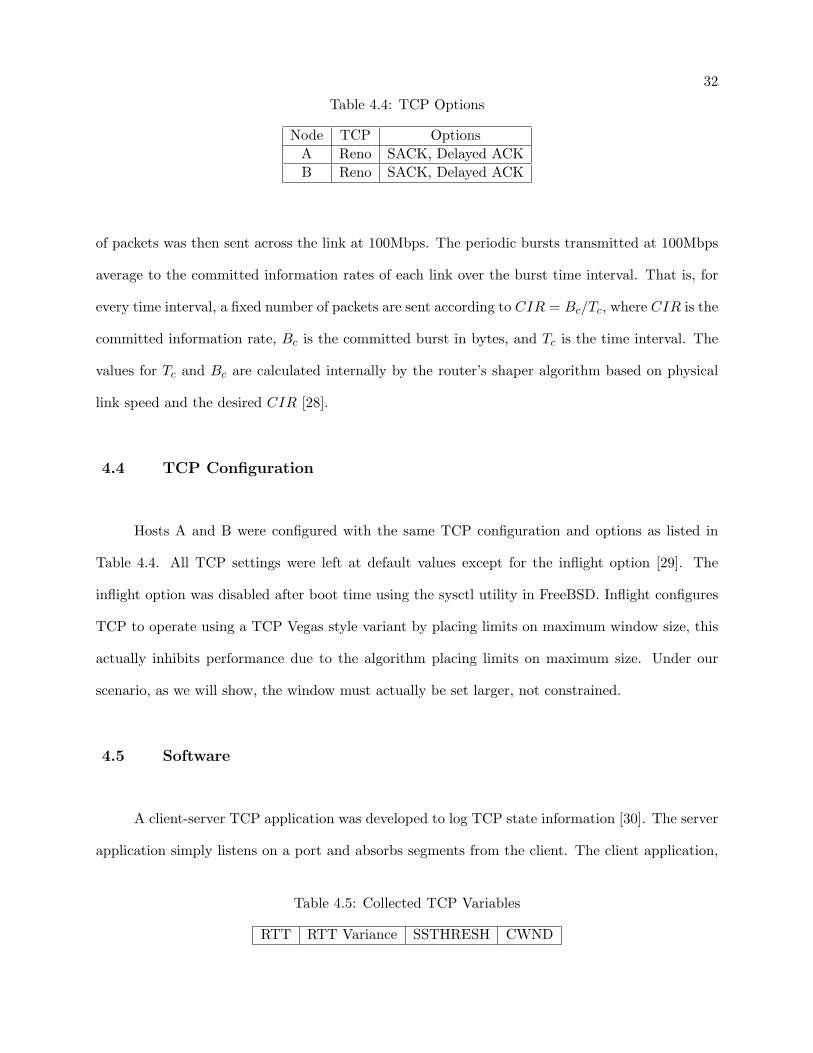
Table 4.4: TCP Options

Node TCP OptionsA Reno SACK, Delayed ACKB Reno SACK, Delayed ACK

of packets was then sent across the link at 100Mbps. The periodic bursts transmitted at 100Mbps

average to the committed information rates of each link over the burst time interval. That is, for

every time interval, a fixed number of packets are sent according to CIR = Bc/Tc, where CIR is the

committed information rate, Bc is the committed burst in bytes, and Tc is the time interval. The

values for Tc and Bc are calculated internally by the router’s shaper algorithm based on physical

link speed and the desired CIR [28].

4.4 TCP Configuration

Hosts A and B were configured with the same TCP configuration and options as listed in

Table 4.4. All TCP settings were left at default values except for the inflight option [29]. The

inflight option was disabled after boot time using the sysctl utility in FreeBSD. Inflight configures

TCP to operate using a TCP Vegas style variant by placing limits on maximum window size, this

actually inhibits performance due to the algorithm placing limits on maximum size. Under our

scenario, as we will show, the window must actually be set larger, not constrained.

4.5 Software

A client-server TCP application was developed to log TCP state information [30]. The server

application simply listens on a port and absorbs segments from the client. The client application,

Table 4.5: Collected TCP Variables

RTT RTT Variance SSTHRESH CWND

33

or TCP sender, opens a socket and emits full size data segments. After each write to the TCP

socket, the client application queries the kernel and gathers TCP state variables listed in Table 4.5

via the TCP_INFO data structure. With each query, a timestamp with microsecond resolution is

sampled and recorded. In addition to state variables, throughput is calculated based on the total

number of bytes written to the socket divided by the total elapsed time.

The client algorithm below details the order of operations used to record TCP state infor-

mation from the client.

while (true)

Record time

Send data

Get TCP state information

Calculate throughput

Write time, state variables, and goodput to log

4.6 Time Synchronization

R1 was configured as an NTP master server [31]. R2 was then configured as a peer. Hosts A

and B used R1 and R2 as NTP servers respectively. This allowed for relative time synchronization

such that TCP state variables could be analyzed accurately for each connection at the same time.

This configuration also minimized the majority of NTP traffic from traversing the asymmetric link

[32].

4.7 Post Processing

Each log file was comprised of a number of tab delimited lines; each containing a timestamp,

and values for RTT, RTT variance, SSTHRESH, CWND, receiver window, sender window, and

34

goodput. The log files for hosts A and B under each run of the experiment were fed into three

Python scripts [33]. The scripts computed a number of values that allowed each connection to be

characterized over time. These values were then run through Gnuplot for observation and further

analysis.

4.7.1 Averages and Ratios

For each run of the experiment, averages of TCP characteristics and throughput for the two

connections were generated using Python scripts. For the download sourced from host A, averages

were generated for the entire connection and for the slice of time where both TCPAB and TCPBA

were active.

Ratios for CWND and throughput were calculated for each buffer size using the previously

calculated averages of the portion of the experiment where both TCPAB and TCPBA were sending

information.

4.7.2 Tcpdump, Wireshark, Mergecap

Tcpdump was run on each host during each experiment. Tcpdump was configured to capture

the first 100B of each frame on the network interface card. After each experiment was finished,

mergecap was run on the capture files from hosts A and B capture files to produce a single pcap

file containing both sessions [34]. Using the merged file, plots of goodput over time could then

generated for TCPAB and TCPBA across a single time axis using Wireshark.

35

4.7.3 Gnuplot

Gnuplot was used to generate all the plots used to explain the interactions between the TCP

connections and buffer sizes in the network [35].

Chapter 5

Results

5.1 Observations

Figure 5.1 shows performance for each asymmetric link combination. It is clear that as

buffer size increases, performance decreases for all asymmetric link configurations. The remainder

of our discussion in this chapter we will focus on the asymmetric link configuration of 12 where

the downlink operates at 2.4Mbps and the uplink operates at 196Kbps. Figures 5.2, 5.3, 5.4 and

5.5 clearly display the goodput degradation of TCPAB and marginal goodput increases in TCPBA

as uplink buffer increases. This behavior is due to TCPAB sizing its window assuming a slowly

changing BDP value and meanwhile TCPBA, in conjunction with the size of BR2, adding large

periodic changes in RTT. The fluctuations in RTT result in BDP changes such that under larger

sizes of BR2, the BDP tracking characteristic of the congestion avoidance algorithm in TCPAB

cannot adapt fast enough to reflect the actual BDP of the link. This leads to the poor goodput of

TCPAB. The concepts are discussed in more detail below.

5.1.1 Connection Synchronization

Connection synchronization for the experiments is shown in Figures 5.6 and 5.7. For small

sizes of BR2, the connections remain out of phase. As BR2 is increased, the synchronization between

TCPAB and TCPBA drifts from out-of-phase towards in-phase. Figures 5.6 and 5.7 display a detail

37

Figure 5.1: Performance for Asymmetric Link Combinations of 3, 12, 30

Figure 5.2: Throughput with 5 Packet Uplink Buffer for 2.4Mbps Downlink and 196Kbps Uplink

Figure 5.3: Throughput with 20 Packet Uplink Buffer for 2.4Mbps Downlink and 196Kbps Uplink

38

Figure 5.4: Throughput with 25 Packet Uplink Buffer for 2.4Mbps Downlink and 196Kbps Uplink

Figure 5.5: Throughput with 50 Packet Uplink Buffer for 2.4Mbps Downlink and 196Kbps Uplink

Figure 5.6: 10 Packet Uplink Buffer - Out of Phase CWND for 2.4Mbps Downlink and 196KbpsUplink

39

Figure 5.7: 50 Packet Uplink Buffer - In Phase CWND for 2.4Mbps Downlink and 196Kbps Uplink

Figure 5.8: 50 Packet Uplink Buffer for 2.4Mbps Downlink and 196Kbps Uplink

40

Figure 5.9: 5 Packet Uplink Buffer for 2.4Mbps Downlink and 196Kbps Uplink

Figure 5.10: 20 Packet Uplink Buffer for 2.4Mbps Downlink and 196Kbps Uplink

41

Figure 5.11: 25 Packet Uplink Buffer for 2.4Mbps Downlink and 196Kbps Uplink

42

of this behavior for BR2 sizes of 10 and 50 respectively. For BR2 equal to 10, the CWND value for

TCPAB drops while the CWND value for TCPBA increases. For BR2 equal to 50, both CWND

values for TCPAB and TCPBA change in the same direction around the same time. Out of phase

synchronization yields higher goodput for TCPAB.

5.1.2 ACK Compression

ACK compression is a phenomenon where a series of ACK segments arrive at a rate that is

larger than the rate at which the corresponding data segments were transmitted. ACK compression

occurs in connection TCPBA. As the BR2 buffer size is increased, ACK compression becomes more

pronounced because a larger amount of ACK segments are queued for longer periods of time and

then subsequently transmitted back to back in a burst. In Figure 5.8 it can be seen that small

sawtooth patterns occur on top of a larger sawtooth pattern. The smaller sawtooth patterns

indicate periods of ACK compression. This is indicated by periods of window growth, followed by

periods of zero transmission.

ACK compression induces bursty TCP behavior. What follows is intermittent periods where

the network is filled with too many packets, resulting in packet loss, TCP throttling, and ultimately,

reduced goodput.

5.1.3 Random and Periodic Connection Interference

When the two connections are active on the network, each experiences interference from the

other. As the size of BR2 increases, the amount of interference also increases, and transforms from

what appears to be a random effect, in Figures 5.2 and 5.3, into a periodic effect, in Figures 5.4,

and 5.5. This periodicity is presumably a result of BR2 filling with TCPBA data segments, thus

delaying enough TCPAB ACKs to stall the connection for periods of time. Table 5.1 lists BR2’s

43

Table 5.1: Uplink Packet Buffer in Packets and Seconds

Packets Seconds5 0.30610 0.61215 0.91820 1.22425 1.53130 1.83735 2.14340 2.44945 2.75550 3.061

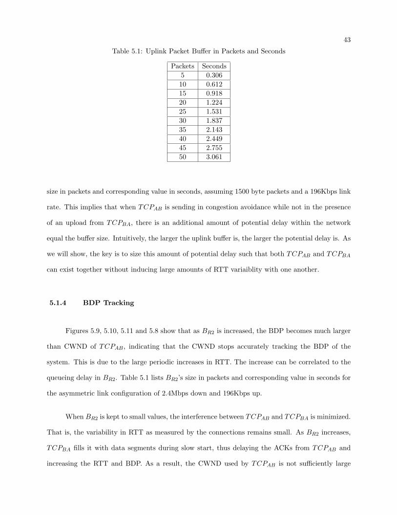
size in packets and corresponding value in seconds, assuming 1500 byte packets and a 196Kbps link

rate. This implies that when TCPAB is sending in congestion avoidance while not in the presence

of an upload from TCPBA, there is an additional amount of potential delay within the network

equal the buffer size. Intuitively, the larger the uplink buffer is, the larger the potential delay is. As

we will show, the key is to size this amount of potential delay such that both TCPAB and TCPBA

can exist together without inducing large amounts of RTT variaiblity with one another.

5.1.4 BDP Tracking

Figures 5.9, 5.10, 5.11 and 5.8 show that as BR2 is increased, the BDP becomes much larger

than CWND of TCPAB, indicating that the CWND stops accurately tracking the BDP of the

system. This is due to the large periodic increases in RTT. The increase can be correlated to the

queueing delay in BR2. Table 5.1 lists BR2’s size in packets and corresponding value in seconds for

the asymmetric link configuration of 2.4Mbps down and 196Kbps up.

When BR2 is kept to small values, the interference between TCPAB and TCPBA is minimized.

That is, the variability in RTT as measured by the connections remains small. As BR2 increases,

TCPBA fills it with data segments during slow start, thus delaying the ACKs from TCPAB and

increasing the RTT and BDP. As a result, the CWND used by TCPAB is not sufficiently large

44

enough to keep the downlink busy when TCPBA is active. We show RTT variability as seen by

host A in terms of standard deviation in Figure 5.12 for each asymmetric link configuration and

uplink buffer size. It is clear that RTT variability increases as buffer size increases. The rate at

which RTT variability increases with respect to buffer size is a function of link asymmetry where

the larger the asymmetry the larger the growth in RTT variability.

5.1.5 Summary

These experiments and results show the impact of buffer size on bi-directional TCP traffic

across asymmetric links, and also begin to demonstrate that a simple solution does in fact exist.

We notice that for buffers of up to a certain size, performance across all of our asymmetric link

combinations remain at high levels. However, once this size is exceeded, performance rapidly drops.

The reason for the drop is related to the large fluctuations in RTT that are induced when the two

TCP connections operate in phase of one another. Therefore, a simple solution exists where as long

as a buffer is less than the threshold, the system will yield significantly higher performance than

it would otherwise. In our next chapter, we will derive an uplink buffer estimation model based

on previous work in [2] that can be used to determine an approximate value for this threshold and

thus, preserve overall system performance.

45

Figure 5.12: Uplink Buffer vs. RTT Variability

Chapter 6

Optimization

6.1 Introduction

In this chapter, a buffer sizing strategy is proposed that constrains maximum RTT and im-

proves goodput for TCPAB while at the same time providing acceptable goodput for TCPBA. This

strategy is beneficial because it does not involve complex queueing algorithms in network elements

and can potentially be implemented locally at the bottleneck link without requiring changes to de

facto TCP implementations in existing operating systems widely used on the Internet. First we

briefly review the factors of bi-directional TCP performance that are influenced by buffer size and

contribute to degraded performance. We then go on to show our buffer sizing strategy and review

its accuracy using data from Section 5.1. Finally we present a procedure for network designers or

operators that can be used on real world networks to ensure uplink buffers are sized such that the

system yields performance values similar to our test network as shown in Table 6.2.

6.2 Review of System Dynamics

As we have previously reviewed, a TCP sender must size its CWND to the BDP of the path

between itself and the receiver in order to fully utilize the link. BDP is calculated via Equation

(2.1) and is composed of bottleneck link line rate and RTT as seen by the sender. As we have

47

Figure 6.1: Test Network RTT Components

shown in Section 5.1, in the scenario where bi-directional TCP traffic is present, the BDP of the

path changes periodically over time and is directly related to uplink buffer size. We have also

reviewed prior work that details the dynamics of bi-directional traffic, specifically how window

sizes of the TCP connections influence the overall performance of the system. The work shows that

if TCP connections remain out of phase, only one direction of the bottleneck link is fully utilized.

In the case of asymmetric links, it is preferred to use more of the downlink than uplink in order to

maximize the performance of the system. As we will show with respect to our test system, sizing

the uplink buffer appropriately limits what phase the two connections operate in, which in turn

limits the variability in RTT, shown in Figure 5.12, and preserves the TCP sender’s ability to track

the BDP of the path while in congestion avoidance mode.

In our system we calculate RTT using Equation (6.1) as shown in Figure 6.1. In Equation

(6.1), let tprop equal total propagation delay, tproc equal total processing delay, and tqueue equal

total queueing delay. Each component of delay can be detailed further as shown in Equations (6.2)

- (6.4).

RTT = tprop + tproc + tqueue (6.1)

tprop = 2 · (propAR1 + propR1R2 + propBR2) (6.2)

tqueue = queueBR1 + queueBR2 (6.3)

tproc = 2 · (procA + procR1 + procR2 + procB) (6.4)

In Equation (6.2), let propAR1 , propR1R2 , and propBR2 equal the propagation delays of the

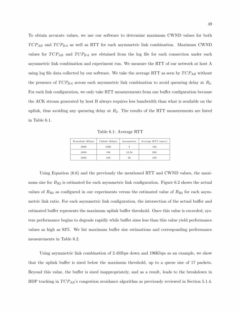
48

links between host A and router R1, R1 and R2, and R2 and host B respectively. In Equation (6.3),

let queueBR1and queueBR2

equal the queueing delay of BR1 and BR2 respectively. In Equation

(6.4), let procA, procB, procR1 , procR2 equal the processing delays at host A, host B, router R1,

and router R2 respectively. These delays are shown in Figure 6.1.

6.3 Uplink Buffer Sizing Model

The dynamics of bi-directional TCP connections involve the RTT and bottleneck rate of the

path and TCP window size. TCP operates in steady state when the RTT of a link is steady. This

allows the congestion avoidance algorithm to accurately track the BDP of the link. If RTT changes

by large amounts, periodically, TCP congestion avoidance mode cannot accurately size its CWND

to reflect the BDP of the path. Therefore, in order to preserve this characteristic, the amount by

which the RTT can change must be limited. As have we shown in Table 5.1, much of the potential

RTT variability is located in empty buffers within the network, BR2 in our network. This implies

that buffers must be sized with care. This has been the topic of significant research, and has led

the tiny model for sizing core router buffers. However, a packet-based buffer sizing strategy for

bi-directional TCP traffic and asymmetric links has yet to be produced.

Beginning with Equation (2.5), a maximum threshold for the uplink buffer is be derived under

which both connections are out of phase, and both can accurately track the BDP of downlink and

uplink. Let WD equal the maximum CWND for TCPAB and WU equal the maximum CWND

for TCPBA. Also, let CD equal the capacity of L21 in bytes, and RTT equal to the total delay

excluding the queueing delay at BR2 in seconds. Finally, let BR2 equal the size of R2’s buffer in

packets.

WD > WU + 2 · (RTT + (BR2 · 1500)/CU ) · CU (6.5)

BR2 < 1/1500 · ((WD −WU )/2−RTT · CU ) (6.6)

49

To obtain accurate values, we use our software to determine maximum CWND values for both

TCPAB and TCPBA as well as RTT for each asymmetric link combination. Maximum CWND

values for TCPAB and TCPBA are obtained from the log file for each connection under each

asymmetric link combination and experiment run. We measure the RTT of our network at host A

using log file data collected by our software. We take the average RTT as seen by TCPAB without

the presence of TCPBA across each asymmetric link combination to avoid queueing delay at R2.

For each link configuration, we only take RTT measurements from one buffer configuration because

the ACK stream generated by host B always requires less bandwidth than what is available on the

uplink, thus avoiding any queueing delay at R2. The results of the RTT measurements are listed

in Table 6.1.

Table 6.1: Average RTT

Downlink (Kbps) Uplink (Kbps) Asymmetry Average RTT (msec)

3000 1000 3 140

2400 196 12.24 200

3000 100 30 160

Using Equation (6.6) and the previously the mentioned RTT and CWND values, the maxi-

mum size for BR2 is estimated for each asymmetric link configuration. Figure 6.2 shows the actual

values of BR2 as configured in our experiments versus the estimated value of BR2 for each asym-

metric link ratio. For each asymmetric link configuration, the intersection of the actual buffer and

estimated buffer represents the maximum uplink buffer threshold. Once this value is exceeded, sys-

tem performance begins to degrade rapidly while buffer sizes less than this value yield performance

values as high as 93%. We list maximum buffer size estimations and corresponding performance

measurements in Table 6.2.

Using asymmetric link combination of 2.4Mbps down and 196Kbps as an example, we show

that the uplink buffer is sized below the maximum threshold, up to a queue size of 17 packets.

Beyond this value, the buffer is sized inappropriately, and as a result, leads to the breakdown in

BDP tracking in TCPAB’s congestion avoidance algorithm as previously reviewed in Section 5.1.4.

50

Figure 6.2: Actual Buffer vs. Estimated Buffer for Asymmetric Link Combinations

51

Table 6.2: Results Summary

Downlink (Kbps) Uplink (Kbps) Asymmetry Estimated Uplink Buffer (Packets) Performance

3000 1000 3 25 0.80

2400 196 12.24 17 0.86

3000 100 30 30 0.68

As shown in Figure 5.1, this results in a continuous drop in system performance, from 86% at our

estimated threshold, to 55% at the largest measured size of BR2.

6.4 Use Case and Procedure

Network designers will find our work useful when incorporating asymmetric links into the

access layer of a network because we present a model and results based on a small number of TCP

connections in either direction, which is a typical traffic pattern found at CPE nodes. Furthermore,

our work presents a simple solution that can be implemented in software on CPE nodes without

introducing additional hardware requirements.

Our work can be used by network designers and operators in two ways. One way is to use our

test methodology, software and estimation model in conjunction with a real world network and set

of hosts as shown in Figure 6.3 to determine appropriate uplink buffer size such that bi-directional

TCP traffic performs at levels shown in our work. In Figure 6.3, let A and B represent TCP hosts.

Let CPE represent the network element terminating the asymmetric link. Let X represent the

downlink and Y represent the uplink. The CPE implements FIFO queueing using a packet based

buffer on its uplink. In the following procedure we refer to this system and demonstrate how to

estimate maximum uplink buffer size.

Figure 6.3: Real World Network with Asymmetric Link Ratio of X / Y

52

(1) RTT: Measure the RTT at a typical TCP sender, A in Figure 6.3, on the network while the

uplink at the CPE, link Y in Figure 6.3, is not congested, thus excluding uplink queueing

delay at the CPE.

To determine the RTT, a download should be launched across the downlink where host

B downloads data from host A. The duration of the download is somewhat arbitrary.

The session should last long enough to determine an appropriate average value. During

the download, RTT measurements should be collected. We present two different ways to

measure RTT.

First, RTT can be measured by capturing the download traffic using Wireshark. In Wire-

shark, set a filter to retain only the TCP download. Once the download has completed, save

the file. Next, browse to the IO Graphs section under the Statistics menu. From here, select

the Y Axis Unit: Advanced option from the drop down menu. Next, choose AVG(*) from

the Calc: section in Graph 1. In the text field next to Calc:, enter tcp.analysis.ack_rtt.

Finally, click the Graph 1 button to generate the plot.

A second way to determine RTT is by using our software and its resulting log file. After

the download between hosts A and B, where A is the TCP sender, has been completed,

the average of all RTT values listed in the second column of the log file can be calculated.

This can be automated using the Download Averaging Script we provide in the Appendix.

(2) Maximum CWND: Next, the uplink buffer on the CPE must be configured to an arbi-

trary value. After the buffer has been configured, a download must be launched using our

software, where host A is the TCP sender. After host A’s TCP connection has entered con-

gestion avoidance, an upload must be launched where host B is the TCP sender. Because

it is not easy to determine what phase a TCP connection is operating in, we recommend

letting the download run for 30 seconds before starting the upload. We then recommend let-

ting the upload and download both run for an additional 30 seconds before terminating the

53

connections. After both connections are terminated, the maximum CWND values should

be extracted from the resultant log files generated by both connections. The Maximum

CWND Script is provided in the Appendix to generate maximum CWND values.

(3) Uplink Buffer Estimation: Now substitute average RTT calculated in step 1 and maxi-

mum CWND values calculated in step 2 into Equation (6.6) to generate a maximum uplink

buffer value. If the uplink buffer provisioned on the CPE is less than this value, it can

be used to keep bi-directional TCP connections out of phase, which in turn, keeps RTT

variability minimized and system performance higher than it would be if the uplink buffer

was sized any larger. If the actual buffer is larger than the estimated buffer, the buffer

should be set to less than the estimated buffer produced by Equation (6.6).

A second way, one that we have not validated and present as future work, is to use data

presented previous work to estimate RTT and CWND values for downloads and uploads. As shown

in previous work, variable delay primarily exists in the access layer of a network because of the

tiny model for buffer sizing in core network elements. This means network designers can accurately

estimate how much RTT variability is in the network based upon buffer sizes and link speeds in

the access network. In addition to this, research also shows that there is an average RTT for TCP

connections traversing the Internet of about 110 msec [27]. Using these two points, it is possible

to estimate an average BDP which in turn can be used to estimate a maximum CWND value.

The estimated RTT and CWND values can then be inserted into inequality (6.6) to determine an

appropriate uplink buffer size for the particular asymmetric link.

6.5 Summary

In this chapter we derive our sizing model and demonstrate its accuracy by comparing its

recommended size to performance results in Section 5.1. In all cases, if buffer size is sized any

larger than our model recommends performance decreases. Under the worse case, where the buffer

54

is sized as large as the uplink, performance drops from 68% at our recommended size to 7% at 50

packets. We also present a use case scenario and accompanying procedure to be used by network

designers and operators to size buffers using our model in asymmetric links for the now common

bi-directional TCP traffic pattern.

Chapter 7

Conclusions

This thesis investigates the effect of buffers on bi-directional TCP connections over asym-

metric links. Previous work focuses on sizing buffers for symmetric links, deriving relationships for

the dynamics of connections and applying novel queueing strategies and TCP adjustments in order

to maintain high levels of goodput. This thesis presents a new approach that solves the problem

by appropriately sizing buffers in asymmetric links.

Experiments were performed on a real network where the uplink buffer, BR2, was varied from

5 packets to 50 packets in increments of 5. Packet traces and TCP state variables were collected

for connection traversing the asymmetric, bottleneck link and then analyzed to show the effect of

buffer size on goodput for both connections.

In summary, by properly sizing buffers, changes in link characteristics that TCP depends

on, such as low packet loss, constant RTT and a steady ACK stream, can be reduced for both

connections, thus optimizing goodput in both directions.

Future work will include additional data on queue length and RTT over time to more clearly

highlight the behavior of each TCP connection. It will also consider how to estimate the desired

buffer size in an online setting. Finally, it will use data reviewed in prior work to validate whether

or not a general case buffer configuration for asymmetric links can be created that aligns with a

common Internet based TCP connection characteristics.

Bibliography

[1] H. Schulze and K. Mochalski, “Internet study 2007,” tech. rep., 2007. www.ipoque.com/userfiles/file/internet_study_2007.pdf.

[2] L. Zhang, S. Shenker, and D. D. Clark, “Observations on the dynamics of a congestion controlalgorithm: the effects of two-way traffic,” SIGCOMM Comput. Commun. Rev., vol. 21, no. 4,pp. 133–147, 1991.

[3] C. Villamizar and C. Song, “High performance TCP in ANSNET,” ACM SIGCOMMComputer Communication Review, vol. 24, no. 5, pp. 45–60, 1994.

[4] M. Heusse, T. X. Brown, T. Schwengler, and A. Duda, “A new look at bidirectional tcpconnections over asymmetric links,” Research Report RR-LIG-002, LIG, Grenoble, France,2010.

[5] H. Balakrishnan, V. Padmanabhan, G. Fairhurst, and M. Sooriyabandara, “TCP PerformanceImplications of Network Path Asymmetry,” IETF RFC 3449, Dec 2002.

[6] V. Cerf and R. Kahn, “A protocol for packet network intercommunication,” IEEE Transactionson Communications, vol. 22, no. 5, 1979.

[7] Linksys, “Linksys BEFVP41 specifications,” 2010. http://homestore.cisco.com/en-us/routers/Linksys-BEFVP41-Wired-Router-Front-Page_stcVVproductId53934564VVcatId552009VVviewprod.htm#.

[8] Linksys, “Linksys CM100 specifications,” 2010. http://homestore.cisco.com/null_stcVVproductId53934565VVcatId552009VVviewprod.htm#.

[9] W. R. Stevens, TCP/IP Illustrated: The Implementation, vol. 2. Addison-Wesley, 1998.

[10] M. Allman, V. Paxson, and W. Stevens, “TCP Congestion Control,” IETF RFC 2581, Apr.1999.

[11] J. Nagle, “Congestion Control in IP/TCP Internetworks,” IETF RFC 896, Jan 1984.

[12] S. Iyer, R. Kompella, and N. McKeown, “Analysis of a memory architecture for fast packetbuffers,” Proceedings of IEEE High Performance Switching and Routing, 2001.

57

[13] A. Vishwanath, V. Sivaraman, and M. Thottan, “Perspectives on router buffer sizing: Recentresults and open problems,” ACM SIGCOMM Computer Communication Review, vol. 39,no. 2, pp. 34–39, 2009.

[14] L. L. Peterson and B. S. Davie, Computer Networks: A Systems Approach. Morgan Kaufmann,4th ed., 2007.

[15] L. Kalampoukas, A. Varma, and K. K. Ramakrishnan, “Two-way tcp traffic over rate controlledchannels: effects and analysis,” IEEE/ACM Trans. Netw., vol. 6, no. 6, pp. 729–743, 1998.

[16] H. Balakrishnan, R. H. Katz, and V. N. Padmanbhan, “The effects of asymmetry on TCPperformance,” Mob. Netw. Appl., vol. 4, no. 3, pp. 219–241, 1999.

[17] F. Louati, C. Barakat, and W. Dabbous, “Handling two-way TCP traffic in asymmetric net-works,” High Speed Networks and Multimedia Communications, pp. 233–243.

[18] L. Kalampoukas, A. Varma, and K. Ramakrishnan, “Improving TCP throughput over two-way asymmetric links: analysis and solutions,” in Proceedings of the 1998 ACM SIGMETRICSjoint international conference on Measurement and modeling of computer systems, pp. 78–89,ACM, 1998.

[19] R. Braden, L. Zhang, S. Berson, S. Herzog, and S. Jamin, “Resource ReSerVation Protocol(RSVP) – Version 1 Functional Specification,” IETF RFC 2205, Sept. 1997.

[20] G. Appenzeller, I. Keslassy, and N. McKeown, “Sizing router buffers,” in SIGCOMM ’04:Proceedings of the 2004 conference on Applications, technologies, architectures, and protocolsfor computer communications, (New York, NY, USA), pp. 281–292, ACM, 2004.

[21] D. Wischik, “Buffer sizing theory for bursty TCP flows,” in Proceedings of the 2006International Zurich Seminar on Communications, pp. 98–101, IEEE Computer Society, 2006.

[22] A. Razdan, A. Nandan, R. Wang, M. Sanadidi, and M. Gerla, “Enhancing TCP performance innetworks with small buffers,” in Computer Communications and Networks, 2002. Proceedings.Eleventh International Conference on, pp. 39–44, 2002.

[23] C. Casetti, M. Gerla, S. Mascolo, M. Sanadidi, and R. Wang, “TCP Westwood: end-to-endcongestion control for wired/wireless networks,” Wireless Networks, vol. 8, no. 5, pp. 467–479,2002.

[24] S. Mascolo and F. Vacirca, “Congestion control and sizing router buffers in the internet,” in44th IEEE Conference on Decision and Control, 2005 and 2005 European Control Conference.CDC-ECC’05, pp. 6750–6755, 2005.

[25] M. Allman, J. Griner, and A. Richard, “TCP behavior in networks with dynamic propagationdelay,” GLOBECOM-NEW YORK-, vol. 2, pp. 1103–1108, 2000.

[26] M. Chan and R. Ramjee, “Improving TCP/IP performance over third-generation wirelessnetworks,” IEEE transactions on mobile computing, vol. 7, no. 4, pp. 430–443, 2008.

58

[27] J. Aikat, J. Kaur, F. Smith, and K. Jeffay, “Variability in TCP round-trip times,” inProceedings of the 3rd ACM SIGCOMM conference on Internet measurement, p. 284, ACM,2003.

[28] Cisco Systems, “Policing and shaping,” Cisco Configuration Guide, 2005. http://www.cisco.com/en/US/docs/ios/qos/configuration/guide/reg_pkt_flow_shaping_ps6350_TSD_Products_Configuration_Guide_Chapter.html.

[29] FreeBSD Project, FreeBSD Handbook. FreeBSD Documentation Project, 2010. http://www.freebsd.org/doc/handbook/.

[30] W. R. Stevens, B. Fenner, and A. M. Rudoff, UNIX Network Programming: The SocketsNetworking API. Addison-Wesley, 3 ed., 2004.

[31] D. Mills, “Network time protocol (version 3) specification, implementation and analysis,”IETF RFC 1305, 1992.

[32] Cisco Systems, “Performing basic system management,” Cisco Configuration Guide, 2007.http://www.cisco.com/en/US/docs/ios/netmgmt/configuration/guide/nm_basic_sys_manage_ps6441_TSD_Products_Configuration_Guide_Chapter.html#wp1001170.

[33] W. Chun, Core Python Programming. Prentice Hall, 2 ed., 2006.

[34] U. Lamping, R. Sharpe, and E. Warnicke, “Wireshark user’s guide,” 2008. http://www.wireshark.org/docs/wsug_html/.

[35] T. Williams and C. Kelley, “Gnuplot 4.4 an interactive plotting program,” 2010. http://www.gnuplot.info/docs_4.4/gnuplot.pdf.

Appendix A

Router Shaper Configuration

R1 Configuration

policy-map R1

class class-default

shape average 2400000

queue-limit 50

!

interface FastEthernet0/0

ip address 192.168.1.1 255.255.255.252

speed 100

duplex full

service-policy R1 out

!

R2 Configuration

policy-map R2

class class-default

shape average 196000

queue-limit <5-50>

60

!

interface FastEthernet0/0

ip address 192.168.1.2 255.255.255.252

speed 100

duplex full

service-policy R2 out

Appendix B

TCP Server

#include <unis td . h>

#include <s t d i o . h>

#include <s t d l i b . h>

#include <s t r i n g . h>

#include <ne t i n e t / in . h>

#include <sys / types . h>

#include <sys / socket . h>

#include <errno . h>

#include <netdb . h>

#include <ne t i n e t / tcp . h>

#include <arpa/ i n e t . h>

#define PORT 5000

int

main ( int argc , char ∗argv [ ] ) {

int tcpsock , sockopt , newsock , pkts , i = 0 ;

int l en = s izeof ( struct t c p i n f o ) ;

struct sockaddr in myaddr , tcpaddr ;

struct t c p i n f o t cp i n f o ;

char buf [ 1 4 6 0 ] ;

bzero(&myaddr , s izeof (myaddr ) ) ;

myaddr . s i n f a m i l y = AF INET ;

myaddr . s in addr . s addr = htonl (INADDR ANY) ;

myaddr . s i n p o r t = htons (PORT) ;

bzero(&tcpaddr , s izeof ( tcpaddr ) ) ;

tcpaddr . s i n f a m i l y = AF INET ;

i f ( ( tcpsock = socket (AF INET , SOCK STREAM, IPPROTO TCP)) < 0)

p r i n t f ( ” socket : %s\n” , s t r e r r o r ( errno ) ) ;

i f ( s e t sockopt ( tcpsock , SOL SOCKET, SO REUSEADDR, &sockopt , s izeof ( sockopt ) ) < 0)

p r i n t f ( ” couldnt s e t opt ions \n” ) ;

i f ( bind ( tcpsock , ( struct sockaddr ∗)&myaddr , s izeof (myaddr ) ) < 0)

62

p r i n t f ( ”bind : %s\n” , s t r e r r o r ( errno ) ) ;

i f ( l i s t e n ( tcpsock , 5) < 0)

p r i n t f ( ” l i s t e n : %s\n” , s t r e r r o r ( errno ) ) ;

i f ( ( newsock = accept ( tcpsock , ( struct sockaddr ∗)&tcpaddr , &len ) ) < 0)

p r i n t f ( ” accept : %s\n” , s t r e r r o r ( errno ) ) ;

for ( ; ; ) {

i f ( read ( newsock , buf , s izeof ( buf ) ) <= 0) {

p r i n t f ( ” read : %s\n” , s t r e r r o r ( errno ) ) ;

c l o s e ( newsock ) ;

return 0 ;

}

}

return 0 ;

}

Appendix C

TCP Client

#include <unis td . h>

#include <s t d i o . h>

#include <s t d l i b . h>

#include <s t r i n g . h>

#include <ne t i n e t / in . h>

#include <sys / types . h>

#include <sys / socket . h>

#include <arpa/ i n e t . h>

#include <ne t i n e t / tcp . h>

#include <errno . h>

#include <netdb . h>

#include <time . h>

#include <sys / time . h>

#define PORT 5000

#define EXTRA TIME 1267500000

int

main ( int argc , char ∗argv [ ] ) {

int tcpsock , sockopt , pkts , i , bytes = 0 , t o t a l b y t e s = 0 ;

int l en = s izeof ( struct t c p i n f o ) ;

double s t a r t t ime = 0 , curt ime = 0 , r e l t ime = 0 ;

f loat throughput ;

struct sockaddr in myaddr , tcpaddr ;

struct t c p i n f o t c p i n f o ;

struct t imeval tv ;

char buf [ 1 4 6 0 ] ;

FILE ∗ fd ;

fd = fopen ( ” t c p s t a t s . txt ” , ”a+” ) ;

i f ( argc == 3)

pkts = a to i ( argv [ 2 ] ) ;

else

pkts = 0 ;

64

bzero(&tcp in fo , s izeof ( t cp i n f o ) ) ;

bzero(&tv , s izeof ( tv ) ) ;

bzero(&myaddr , s izeof (myaddr ) ) ;

myaddr . s i n f a m i l y = AF INET ;

myaddr . s in addr . s addr = htonl (INADDR ANY) ;

myaddr . s i n p o r t = htons ( 0 ) ;

bzero(&tcpaddr , s izeof ( tcpaddr ) ) ;

tcpaddr . s i n f a m i l y = AF INET ;

tcpaddr . s i n p o r t = htons (PORT) ;

i f ( i n e t p ton (AF INET , argv [ 1 ] , &tcpaddr . s in addr ) <= 0) {

p r i n t f ( ” could not copy ip to address s t ru c tu r e \n” ) ;

return 1 ;

}

i f ( ( tcpsock = socket (AF INET , SOCK STREAM, 0) ) < 0)

p r i n t f ( ” socket : %s\n” , s t r e r r o r ( errno ) ) ;

i f ( s e t sockopt ( tcpsock , SOL SOCKET, SO REUSEADDR, &sockopt , s izeof ( sockopt ) ) < 0)

p r i n t f ( ” couldnt s e t opt ions \n” ) ;

i f ( connect ( tcpsock , ( struct sockaddr ∗)&tcpaddr , s izeof ( tcpaddr ) ) < 0)

p r i n t f ( ” connect : %s\n” , s t r e r r o r ( errno ) ) ;

f p r i n t f ( fd , ”%s\ t%s\ t%s\ t%s\ t%s\ t%s\ t%s\ t%s\ t%s\n” ,

”Time” ,

”RTT” ,

”RTT Var” ,

”SSTHRESH” ,

”CWND” ,

”Rcv Wnd” ,

”Snd Wnd” ,

”Snd BW Wnd” ,

”Throughput” ) ;

i f ( pkts != 0) {

for ( i = 0 ; i <= pkts ; i++) {

gett imeofday(&tv , NULL) ;

curt ime = (double ) tv . t v s e c + (double ) tv . tv usec /1000000 − EXTRA TIME;

i f ( bytes == 0)

s ta r t t ime = curtime ;

r e l t ime = curtime − s t a r t t ime ;

i f ( ( bytes = wr i t e ( tcpsock , buf , s izeof ( buf ) ) ) < 0)

p r i n t f ( ” wr i t e : %s\n” , s t r e r r o r ( errno ) ) ;

t o t a l b y t e s += bytes ;

throughput = ( t o t a l b y t e s ∗ 8)/ r e l t ime ;

65

i f ( getsockopt ( tcpsock , IPPROTO TCP, TCP INFO, (void ∗)& tcp in fo , ( s o c k l e n t ∗)& len ) == −1)

p r i n t f ( ” getsockopt : %s\n” , s t r e r r o r ( errno ) ) ;

f p r i n t f ( fd , ”%f \ t%u\ t%u\ t%u\ t%u\ t%u\ t%u\ t%u\ t%f \n” ,

curtime ,

t c p i n f o . t c p i r t t ,

t c p i n f o . t c p i r t t v a r ,

t c p i n f o . t c p i s n d s s t h r e s h ,

t c p i n f o . tcpi snd cwnd ,

t c p i n f o . t cp i r c v spa c e ,

t c p i n f o . tcpi snd wnd ,

t c p i n f o . tcpi snd bwnd ,

throughput ) ;

}

}

else {

for ( ; ; ) {

gett imeofday(&tv , NULL) ;

curt ime = (double ) tv . t v s e c + (double ) tv . tv usec /1000000 − EXTRA TIME;

i f ( bytes == 0)

s ta r t t ime = curtime ;

r e l t ime = curtime − s t a r t t ime ;

i f ( ( bytes = wr i t e ( tcpsock , buf , s izeof ( buf ) ) ) < 0)

p r i n t f ( ” wr i t e : %s\n” , s t r e r r o r ( errno ) ) ;

t o t a l b y t e s += bytes ;

throughput = ( t o t a l b y t e s ∗ 8)/ r e l t ime ;

i f ( getsockopt ( tcpsock , IPPROTO TCP, TCP INFO, (void ∗)& tcp in fo , ( s o c k l e n t ∗)& len ) == −1)

p r i n t f ( ” getsockopt : %s\n” , s t r e r r o r ( errno ) ) ;

f p r i n t f ( fd , ”%f \ t%u\ t%u\ t%u\ t%u\ t%u\ t%u\ t%u\ t%f \n” ,

curtime ,

t c p i n f o . t c p i r t t ,

t c p i n f o . t c p i r t t v a r ,

t c p i n f o . t c p i s n d s s t h r e s h ,

t c p i n f o . tcpi snd cwnd ,

t c p i n f o . t cp i r c v spa c e ,

t c p i n f o . tcpi snd wnd ,

t c p i n f o . tcpi snd bwnd ,

throughput ) ;

}

}

c l o s e ( tcpsock ) ;

f c l o s e ( fd ) ;

return 0 ;

}

Appendix D

Bandwidth Delay Product Estimation Script

#! / usr / b in / env python

import sys

bwdStats = open ( sys . argv [ 3 ] , ”a” )

myFile = open ( sys . argv [ 1 ] , ”rU” )

l inkSpeed = in t ( sys . argv [ 2 ] )

for aRow in myFile :

i f aRow . s p l i t ( ’\ t ’ ) [ 0 ] == ”Time” :

continue

else :

bwd = l inkSpeed ∗ f l o a t (aRow . s p l i t ( ’\ t ’ ) [ 1 ] ) / 8000000

myList = [ f l o a t (aRow . s p l i t ( ’\ t ’ ) [ 0 ] ) , bwd ]

for i , j in enumerate ( myList ) :

bwdStats . wr i t e ( repr ( j )+ ’\ t ’ )

bwdStats . wr i t e ( ’\n ’ )

myFile . c l o s e ( )

bwdStats . c l o s e ( )

Appendix E

Download Averaging Script

#! / usr / b in / env python

import sys

t cpStat s = open ( sys . argv [ 5 ] , ”a” )

myFile = open ( sys . argv [ 1 ] , ”rU” )

cwnd = 0.0

r t t = 0 .0

i = 0 .0

j = 0 .0

downcwnd = 0.0

downrtt = 0 .0

for aRow in myFile :

i f aRow . s p l i t ( ’\ t ’ ) [ 0 ] == ”Time” :

continue

e l i f f l o a t (aRow . s p l i t ( ’\ t ’ ) [ 0 ] ) > i n t ( sys . argv [ 2 ] ) :

cwnd+=f l o a t (aRow . s p l i t ( ’\ t ’ ) [ 4 ] )

r t t+=f l o a t (aRow . s p l i t ( ’\ t ’ ) [ 1 ] )

i+=1

else :

downcwnd+=f l o a t (aRow . s p l i t ( ’\ t ’ ) [ 4 ] )

downrtt+=f l o a t (aRow . s p l i t ( ’\ t ’ ) [ 1 ] )

j+=1

avgDownCWND = downcwnd/ j

avgDownRTT = downrtt/ j

avgDownThroughput = (avgDownCWND ∗ 8) / (avgDownRTT / 1000000)

avgCWND = cwnd/ i

avgRTT = r t t / i

avgThroughput = (avgCWND ∗ 8) / (avgRTT / 1000000)

difThroughput = avgDownThroughput − avgThroughput

difRTT = avgRTT − avgDownRTT

avgBWD = (avgRTT / 8000000) ∗ i n t ( sys . argv [ 3 ] )

diffWND = avgBWD − avgCWND

di f fThpt = (diffWND ∗ 8) / (avgRTT / 1000000)

68

print ”Average CWND:\ t%f ” % avgCWND

print ”Average Down CWND:\ t%f ” % avgDownCWND

print ”Average Throughput :\ t%f ” % avgThroughput

print ”Average Download Throughput :\ t%f ” % avgDownThroughput

print ”Throughput D i f f e r e n c e :\ t%f ” % difThroughput

print ”Average RTT:\ t%f ” % avgRTT

print ”Average Download RTT:\ t%f ” % avgDownRTT

print ”RTT D i f f e r e n c e :\ t%f ” % difRTT

print ”Average BW∗D:\ t%f ” % avgBWD

print ”Window D i f f e r e n c e :\ t%f ” % diffWND

print ” Id ea l Thpt D i f f e r e n c e :\ t%f ” % di f fThpt

myList = [ i n t ( sys . argv [ 4 ] ) , avgCWND, avgDownCWND, avgThroughput , avgDownThroughput ,

difThroughput , avgRTT, avgDownRTT, difRTT , avgBWD]

for i , j in enumerate ( myList ) :

t cpStat s . wr i t e ( repr ( j )+ ’\ t ’ )

t cpStat s . wr i t e ( ’\n ’ )

myFile . c l o s e ( )

t cpStat s . c l o s e ( )

Appendix F

Upload Averaging Script

#! / usr / b in / env python

import sys

t cpStat s = open ( sys . argv [ 3 ] , ”a” )

myFile = open ( sys . argv [ 1 ] , ”rU” )

i = 0

cwnd = 0

r t t = 0

for aRow in myFile :

i f aRow . s p l i t ( ’\ t ’ ) [ 0 ] == ”Time” :

continue

else :

cwnd += f l o a t (aRow . s p l i t ( ’\ t ’ ) [ 4 ] )

r t t += f l o a t (aRow . s p l i t ( ’\ t ’ ) [ 1 ] )

i+=1

avgCWND = cwnd/ i

avgRTT = r t t / i

avgThroughput = (avgCWND ∗ 8) / (avgRTT / 1000000)

myList = [ i n t ( sys . argv [ 2 ] ) , avgCWND, avgThroughput , avgRTT ]

for i , j in enumerate ( myList ) :

t cpStat s . wr i t e ( repr ( j )+ ’\ t ’ )

t cpStat s . wr i t e ( ’\n ’ )

t cpStat s . c l o s e ( )

myFile . c l o s e ( )

Appendix G

Maximum CWND Script

#!/ usr / b in / env python

#1 i n f i l e

#2 o u t f i l e

#3 b u f f e r

import sys

myFile = open ( sys . argv [ 1 ] , ”rU” )

tcpStat s = open ( sys . argv [ 2 ] , ”a” )

cwnd = 0.0

for aRow in myFile :

i f aRow . s p l i t ( ’\ t ’ ) [ 0 ] == ”Time” :

continue

else :

i f cwnd < f l o a t (aRow . s p l i t ( ’\ t ’ ) [ 4 ] ) :

cwnd = f l o a t (aRow . s p l i t ( ’\ t ’ ) [ 4 ] )

print ”Max CWND: %f ” % cwnd

myList = [ i n t ( sys . argv [ 3 ] ) , cwnd ]

for i , j in enumerate ( myList ) :

t cpStat s . wr i t e ( repr ( j )+ ’\ t ’ )

t cpStat s . wr i t e ( ’\n ’ )

myFile . c l o s e ( )

t cpStat s . c l o s e ( )