understanding modeling and managing longevity risk

8/14/2019 Understanding Modeling and Managing Longevity Risk

http://slidepdf.com/reader/full/understanding-modeling-and-managing-longevity-risk 1/35

Submitted to Operations Research manuscript (Please, provide the mansucript number!)

Understanding, Modeling and ManagingLongevity Risk: Key Issues and Main

Challenges*Pauline Barrieu

Statistics Department - London School of Economics

Harry BensusanCentre de Mathematiques Appliquees - Ecole Polytechnique

Nicole El KarouiCentre de Mathematiques Appliquees - Ecole Polytechnique

Caroline HillairetCentre de Mathematiques Appliquees - Ecole Polytechnique

Stephane LoiselUniversite de Lyon, Universite Claude Bernard Lyon 1

Institut de Science Financiere et d’Assurances

Claudia RavanelliEcole Polytechnique Federale de Lausanne

Yahia SalhiUniversite de Lyon, Universite Claude Bernard Lyon 1

Institut de Science Financiere et d’Assurancesand

R&D Longevity-Mortality, SCOR Global Life

In this article we investigate the latest developments on longevity risk modeling. We rst introduce longevityrisk and some key actuarial denitions as to allow for a better understanding of the related challenges in termof risk management from both a nancial and insurance point of view. The article also provides a global viewon the practical issues on longevity-linked insurance and pension funds products that arise mainly from thesteady increase in life expectancy since 1960s. Those issues are leading the industry to adopt more effectiveregulations to better assess and efficiently manage the inherited risks. Simultaneously, the development onthe longevity has enhanced the need of capital markets as to manage and transfer the risk throughout theso-called insurance-linked securities (ILS). Therefore, we also highlight future developments on longevityrisk management from a nancial point of view, bringing up practices from the banking industry in termsof modeling and pricing.

Key words : Longevity Risk, securitization, risk transfer, incomplete market, life insurance, stochasticmortality, pensions, long term interest rate, regulation, population dynamics.

* The authors of this paper are members of the working group on longevity risk with nancial supportof Federation Bancaire Fran¸ caise.

1



Barrieu et al.: Understanding, Modeling and Managing Longevity Risk 2 Article submitted to Operations Research ; manuscript no. (Please, provide the mansucript number!)

The observed constant improvements in longevity are bringing new issues and chal-lenges at various levels: social, political, economic and regulatory to mention only afew. But one of the most publicized impacts of longevity improvements is certainlyon pensions. In 2009, in most developed countries, many companies have closed thedened benet retirement plans (such as the 401(K) plans in the United States) that

they used to offer to their employees. Such a scheme represents indeed a risk trans-fer from both the industry and the insurers back to the policyholders, which, from asocial point of view, is not satisfactory anymore. Similarly, in several countries, denedbenet pension plans have been continuously replaced with dened contribution plans,leading to the same result. In addition, some governments are about to increase theretirement age by 2 or 5 years to take into account longevity improvements, populationageing and the nancing of pension.The insurance industry is also facing some specic challenges related to longevity risk,i.e. the risk that the trend of longevity improvements signicantly changes in the future.More and more capital has to be constituted to face this long-term risk, and newregulations in Europe, together with the recent nancial crisis only amplify this phe-nomenon. Hence, it has become more and more important for insurance companies andpension funds to nd a suitable and efficient way to cross-hedge or to transfer part of the longevity risk to reinsurers or to nancial markets. Longevity risk is however notso easy to transfer, as it is hard to understand, and therefore to manage. In particular,because of its long-term nature, accurate longevity projections are delicate and mod-eling the embedded interest rate risk remains challenging.As to better manage longevity risk, prospective life tables, containing longevity trendprojections are used. They prove to be very helpful for reserving in life insurance in par-ticular but the irregular updates of these tables can cause some problems. For instance,the French prospective life tables were updated in 2006. As longevity improvementswere more important than expected according to the previous prospective tables estab-lished in 1993, French insurers had to increase their reserves by 8% on average toaccount for this phenomenon! Moreover, in addition to this risk of observing a signi-cant change in the longevity trend, the insurance sector is facing some basis risk as theevolution of the policyholders mortality is usually different from that of the nationalpopulation, because of some selection effects. This selection effect has different impactson different insurance companies portfolios, as mortality levels, speeds of decrease andaccelerations are very heterogeneous in the insurance industry. This makes it hard forinsurance companies to rely on national indices or even on industry indices to managetheir own longevity risk.To better understand the longevity risk and avoid some managerial over-reactionsdue to short-term oscillations around the average trend, the dynamics of longevityimprovements, their causes, and the above mentioned heterogeneity have to be studiedcarefully. Many standard stochastic models for mortality have been developed, some of

them inspired by the classical credit risk and interest rates literature. In these models,mortality is mainly explained by age and time. An alternative approach consists of amicroscopic modeling for a population where individuals are characterized not only bytheir age but also by other features reecting their living conditions. Such models arevery useful for the risk analysis of a given insurance portfolio, but also at a social andpolitical level when combined with a study of other demographic rates, such as fertil-ity and immigration rates: projective scenarii can guide the strategies of governments



Barrieu et al.: Understanding, Modeling and Managing Longevity Risk Article submitted to Operations Research ; manuscript no. (Please, provide the mansucript number!) 3

concerning bills on immigration and on the age of retirement for example.The European insurance industry will soon have to comply to some new solvency reg-ulations, namely Solvency II. Those regulations and standards lay the emphasis onthe way risks endorsed by an insurance company should be handled in order to faceadverse economic and demographic situations. Those regulations will be effective by

late 2012 and certainly enhance the development of alternative risk transfer solutionsfor insurance risk in general and for longevity risk in particular.No doubt that the pricing methodologies for insurance related transactions, and in par-ticular longevity linked securities will be impacted as more and more alternative solu-tions appear in the market. Today, the longevity market is an immature and incompletemarket, with an evident lack of liquidity. Standard replication strategies are impossi-ble, making the classical nancial methodology not applicable. In this case, indifferencepricing, involving utility maximization, seems to be a more appropriate point of viewto adopt. Besides, due to the long maturities of the underlying risk, the modeling of long term interest rate becomes also unavoidable and adds to the complexity of theproblem.Our paper is organized as follows: we rst describe the main characteristics of longevityrisk, insisting on the classical and prospective life tables and mortality data, and somespecic features such as the cohort effect. In Section 2, we present the key models formortality risk and how they can be used to model longevity risk. Section 3 is dedicatedto the new solvency regulations that will be enforced by 2012 and discuss in particularlongevity risk management. In Section 4, we are concerned with longevity risk transferissues and the convergence between the insurance industry and the capital markets.Finally, we look at the main modeling questions regarding the pricing of longevity risk,with a discussion on long term interest rates modeling.

1. Characteristics of longevity riskIn this rst section, we introduce some fundamental notions related to longevity risk.

In particular, we give some basics on life tables, including the standard notation usedboth in practice and in the literature, and detail some noticeable features such as thecohort effect.

1.1. Mortality and longevity data

1.1.1. Life tables for mortality risk To analyze variations of mortality acrossdifferent age classes and to take into account various factors (e.g. infant mortality,ageing, accidents,...), actuaries have been using life tables, also called mortality tables.Classical life tables usually have two entries: the rst one corresponds to the age x∈N ,the second one, denoted by lx , seems to stand at rst sight for the number of survivorsat age x.

It is important however to understand that the population under study is in fact actitious one and that those survivors do not exist in real world. During a speciccommon observation period (from 1995 to 2000 inclusive, say) the probability to diebetween two ages (usually x and x + 1, or x and x + 5) is estimated. Let us givemore details on this point: for each x ∈N (up to the maximal age, for example 120years), ignoring for the sake of clarity both censored data (i.e. when the time of deathof individuals is not known precisely) and truncated observations, let us consider the




number lx of individuals who turn age x between 1st of January 1995 and 1st of January2000. Assume that dx out of those lx individuals will die between age x and x +1. Theannual mortality rate qx at age x is the probability for someone aged x to die withinone year and may be estimated by d x

l x. Of course, in practice, an individual born in

early January 1914 would only be ”observed” during a few days between ages 80 and

81 during the period 1995-2000 (as this person would turn 81 in early January 1995).Some people may change country or purchase another policy and stop being observedbefore the end of the observation period and age x +1. Actuaries will take into accountthese types of reduced observations using some classical statistical tools such as theKaplan-Meier estimator (see Klein and Moeschberger (2003))Internal data in insurance companies usually enables actuaries to estimate the full butstill ctitious survival function S dened by

S (x) = P (τ > x )

for x ≥ 0 (but not necessarily in N ), where τ is the random lifetime of a member of this virtual population and P is the statistical probability measure.In a similar way, national data only consists of pictures of the population every year.

Starting from national life table which produce estimates for S (x) for x ∈N

, it isthen necessary to make some additional arbitrary assumptions to reconstruct the fullsurvival function. In practice, actuaries assume that the mortality force µ(x) (or thehazard rate of S ) at any age x ≥ 0, dened as

µ(x) = −d(ln S )

dx(x), (1.1)

is either locally constant or admits a certain local parametric form (in accordanceto Gompertz or Makeham survival functions), or that mortality rates follow someproperties (see for example Denuit and Delwaerde (2005)).In some cases, an alternative mortality rate, called the central mortality rate, is usedinstead of annual mortality rates in order to take into account the fact that after therst deaths, the size of the population has decreased, and so the following deaths willhave a heavier weight in the estimation. As to dene this adjusted mortality rate,we need to introduce rst the notion of exposure to risk, which refers to the averagenumber of individuals in the population over a calendar year adjusted for the lengthof time they are in the population. The exposure to risk is dened as:

ET R x = 1

0lx + u du.

The central mortality rate is then dened as:

m x =lx − lx +1

ET R x.

Using some standard passage formulae, we can obtain a relationship between the var-

ious quantities qx , m x and µx , depending on the previous assumptions.Note that classical life tables are well-suited to quantify short-term mortality risk(death insurance), for time horizons from 1 to 5 years provided that no exceptionalevent occurs (such as pandemic or heat wave). On the contrary, these tables are notrelevant for reserving issues regarding long term longevity-based contracts like annu-ities or pensions, as mortality rates are changing over time and one must take thisevolution into account.




1.1.2. Data for longevity risk When looking at longevity risk, it is necessaryto quantify not only the level of mortality rates, but also their evolution in time. To beable to elaborate prospective life tables (as detailed in the subsequent Subsection 2.1)and take into account the evolution of mortality over time, one must rst collect mor-tality data during different periods of time or regarding different cohorts (also called

generations) to answer the following questions. What is exactly a life table for thegeneration t0 (i.e. for individuals born in year t0)? First, note that in year t, the deathof survivors at ages larger than t − t0 + 1 is not observed (as those events would occurafter year t +1) and can only be estimated using some projections (see Subsection 2.1).Second, how should one understand the mortality rate at age x during calendar year t(denoted by qx,t )? How to dene mortality parameters?To illustrate this last point, let us focus on a particular example. We would like todene and estimate q65 ,2008 . To do so, we start by estimating the probability q65 ,2008;1942

that an individual born in 1942 (aged in average between 65 .5 years on 1st of January2008) dies during her 66th year in 2008 (being exposed ages 65 .5 and 66 in average),and the probability q65 ,2008;1943 that an individual born in 1943 (aged in average 64 .5on 1st of January 2008) dies during her 66th year in 2008 (being exposed between ages65 and 65.5). Under some assumptions on mortality rates, one denes

q65 ,2008 = 1 − (1 − q65 ,2008;1943 )(1 − q65 ,2008;1942 ),

from the so-called Lexis diagram (see Figure 1.1).Note that

q65 ,2008;1942 =d(65, 2008;1942)

p(65, 2008)and q65 ,2008;1943 =

d(65, 2008;1943) p(65, 2009)+ d(65, 2008;1943)

,

where d(x, y ; g) corresponds to the number of individuals born in year g and deceasedduring year y between age x and age x + 1, and p(x, y) corresponds to the numberof survivors with age between x and x + 1 on 1st of January of year y (born duringyear y − x − 1). Using national data (as we only have at our disposal the size of thepopulation for each age and the number of deaths), the central mortality rates can onlybe obtained after some assumptions on the distribution for the death times, becauseof the exposure to risk. Assuming that the mortality force µ(x, t ) is constant on eachbox of the Lexis diagram, note that central mortality rates and mortality forces areidentical 1 . It is then possible to dene the probability to survive T − t additional years(up to date T ≥ t) for someone aged x at time t as:

S t (x, T ) = P t (τ > x + ( T − t) | τ > x ) = e− T t µ (x + s − t,s )ds . (1.2)

These approximations are reasonable when studying average trends or making projections. Indeed, in practice, except for high ages, ln µx,t , ln m x,t and logit qx,t

2 arequite similar. Nevertheless, if one wants to quantify the size of oscillations around the

1 This is the reason why the Lee-Carter model (presented in details in Section 2.1), which was initiallyformulated by Lee and Carter (1992) for central mortality rates, has been used by many actuaries andstatisticians (e.g. Denuit and Delwaerde (2005 )) for mortality forces.2 The logit function is dened as logit ( x )=ln(

x

1 − x) .




C o h o

r t

Year

Age

66

65

64

63

200819431942

Figure 1.1 Lexis diagram: This is an age-year-cohort diagram representing the evolution of mor-tality over time. The real cohort mortality is followed on a diagonal manner and thectitious (also called period) cohort could be read vertically. For example, the blackcircle corresponds to death of an individual, born in 1943, in 2008. The circle is situatedon the upper triangle of the death year 2008 box (the grey box), meaning that theindividual died in late 2008, say at age 64 . 61.

1840 1860 1880 1900 1920

3 0

4 0

5 0

6 0

7 0

year

1840 1860 1880 1900 1920

4 0

4 5

5 0

5 5

6 0

6 5

7 0

year

Figure 1.2 Periodic life expectancy (left) and generational life expectancy (right) at birth in theUK.




trend and try to detect changes in the trend, these approximations may deterioratethe results. Besides, these measures of the mortality rate qx,t are sensitive to somesources of randomness apart from the longevity risk: for example, if there are changesin natality in the year of birth, additional articial oscillations may be observed. Thisphenomenon exists but can be neglected outside wars or periods of important economic

difficulties.Insurance companies have much more detailed information: they know the exact ageof the policyholders and they observe (almost) exact death instants. This may allowthem to test various assumptions, such as constant interest force on each box of theLexis Diagram. However, the limited size of their portfolios (in comparison to nationalpopulations) is a clear drawback.

1.2. Period and cohort tables and effects

As briey mentioned earlier, prospective life tables may be constructed and presentedeither by cohort or by period. To emphasize once more the ctitious nature of periodlife tables, let us compare retrospective life expectancy at birth for English and Welshmales obtained from period tables and cohort tables from the period 1840 to 1925 (seeFigure 1.2): on the left-hand side, due to the rst World War, mortality rates increasefor all adult ages from 1914 to 1917, reaching a peak in 1918 due to the u pandemic.The consequences on the life expectancy (computed from annual period tables) arevery strong: life expectancy at birth is around 32 years in 1918, instead of 51 years in1919! The reason for this extreme uctuation is that period life expectancy at birth in1918 is obtained from annual mortality rates observed at each age during year 1918: itwould correspond to the life expectancy for individuals who would spend their wholelife with ”pandemic-style” mortality and with no longevity improvement. This hasnothing to do with the cohort view (life expectancy at birth is around 60 years for 1918and 1919 cohorts). The values of period life expectancy at birth for periods 1918 and

1919 point out the fact that one must be very cautious with period-based longevityindices to avoid over-reactions and as a consequence basis risk. Nevertheless, it maybe adapted and it is sometimes preferable to make prospective tables by extrapolatingperiod mortality tables, provided that the consistency of the deduced cohort-basedtables is preserved. Alternate solutions are to extrapolate directly cohort tables usingdiagonal-wise projections, or to use age-period-cohort approaches to take both thecohort and the period effects into account.The cohort effect refers to historical factors that are specic to a year of birth (suchas the introduction of new drugs or vaccines), or to a group of birth years (such assmoking habits or women’s professional activity level). It may be hard to perceive thiseffect as individuals are primarily involved in time and age dynamics, and at a lowerlevel undergoing the consequences of their belonging to a certain generation, even if some cohort or cohort-group specic mortality patterns are striking, particularly in theUnited Kingdom. Only longevity improvements that are observed between two cohorts,for most periods and ages, correspond to the cohort effect. On the contrary, a heat waveand the fact that new medicine is available for adults correspond to period effects. Inpractice, the continuum of longevity improvements makes it difficult to isolate cohorteffect and period effect, which can signicantly intercept each other.




1.3. Smoothing and closing tables

Age proles of empirical annual mortality rates (based on yearly published nationalstatistics) are inconsistent for high ages (see Figure 1.3). The older, the moreinconsistent the results are. This is the reason why actuaries usually close mortalitytables, i.e. extrapolate the shape of the survival functions at high ages from someexogenous assumptions. Besides, in each country, annual population size estimationsare done only up to a certain age. In France this maximal age is 100. In the past,mortality after age 100 was not a very important point and had a very small impacton residual life expectations (and so annuities) for workers or young retirees. With therecent longevity improvements, this is no longer the case, and it becomes important tohave a better view on mortality and longevity risk for high ages, because this part of the population has a heavier weight but also because the mortality is now improvingfor those ages.Up to now, after estimating bulk mortality rates, actuaries smooth empirical life tablesup to age 90, and then close the table by using a local parametric shape and by takingsome exogenous assumptions for parameter tting (such as the central mortality rateat age 115 is 1, or the residual life expectation at age x is 2, etc...). This processis illustrated in Figure 1.3 for mortality rates of English males. For age-cohort orage-period models, the problem is more difficult as surfaces (instead of curves) haveto be smoothed.

70 80 90 100 110 120 130

0 . 0

0 . 2

0 . 4

0 . 6

0 . 8

1 . 0

age

m o r t a

l i t y r a

t e s

Actual mortalitySmoothed mortality

Figure 1.3 Smoothing and closing life tables

1.4. Heterogeneity, revisions, migrations, indices

Longevity patterns and longevity improvements are very different from one companyportfolio to the other, and even for different countries. This variability is very important




for longevity risk transfer, as basis risk may be too important for insurers to acceptto use nancial instruments based on national indices to hedge their longevity risk, asthis hedge would be too imperfect (see Section 4). Guarantees could also be based onnational industry indices, but the problem is then that those indices and projectionsare revised too seldom.

To take into account national or entity specic mortality data, one would also needto collect more accurate information on migrations, which is not always easy. Thisis of course not always possible due some restrictions to access to those informationdepending on the migration politics of the underlying country.The discrepancies between countries and portfolios (due to socio-economic factors,health, differences between males and females, migrations, ...) make every longevitystudy specic. Even if some common features may exist, this heterogeneity makesit difficult to jointly model longevity risks contained in different portfolios and toaggregate them without additional work.

2. Modeling longevity risk

Prospective life tables provide a view on the future evolution of mortality rates. Indeed,in most developed countries (apart from Russia), longevity has been improving forseveral decades and a simple look at the standard life tables, as we introduced above,is more restrictive and can underestimate the real evolution of future mortality. Theprospective life tables offers a better view of the mortality evolution. Consequently,estimating mortality rate at age 70 from individuals who had this age in the pastusually underestimates the probability of a person who is 50 years old today and whoreaches age 70 to survive one more year. Prospective life tables may be dened forcalendar years, or for cohorts (per year of birth). Every year, the various nationalinstitutes (INSEE in France, Bureau of Census in the US, CMI in the UK, ...) publishthe level of national mortality through annual mortality rates. This is the data usedby LifeMetrics and other providers of longevity indices as described in Section 4. It isalso possible to obtain mortality data for most developed countries using the HumanMortality Database (HMD). The HMD is a free 3 database launched in 2002 by theDepartment of Demography at the University of California, Berkeley, USA and theMax Plank Institute for Demographic Research in Rostock, Germany. This databaseprovides detailed mortality and population data to those interested in the history of human longevity.Life tables and prospective life tables can also be built from entity-specic data, e.g.insurance companies or pension funds. For those entities, mortality may strongly dif-fer from that of the national population due to the selection effect. Nevertheless, it isoften very difficult to construct entity-specic prospective life tables without any refer-ence to one or several national references. As an example, the last market-wide French

prospective life tables, constructed in 2006, were produced on the basis of 700000 indi-viduals from 19 different insurance companies and mutual companies. Even groupingthese 19 insurance portfolios did not provide enough data to avoid the necessity touse a national reference. Actuaries usually try to nd an appropriate link betweenthe level of mortality and the longevity improvements of the portfolio, and the ones

3 available at http://www.mortality.org

http://www.mortality.org/

http://www.mortality.org/




of the national population(s), thanks to so-called relational models (see Denuit andDelwaerde (2005)). But quantifying longevity basis risk remain very difficult.

a g e

20

40

60

80

100

c a l e n d a r y e a r

1970

1980

1990

2000

g − m o r t a l i t y

r a t e −8

−6

−4

−2

0 20 40 60 80 100

− 1 0

− 8

− 6

− 4

− 2

0

Age

L o g −

m o r t a

l i t y r a

t e

Figure 2.1 Log-mortality structure of French male, 1962-2000

2.1. Some standard models

2.1.1. Mortality models A variety of models have been introduced, startingwith the famous Lee-Carter model ( Lee and Carter (1992)), widely used by insurancepractitioners. We can also name among others, the Renshaw-Haberman model ( Ren-shaw and Haberman (2006, 2003)) that incorporates for the rst time a cohort effectparameter to characterize the observed variations on mortality among individuals froma different cohort. A detailed survey on the classical mortality models has been carriedby Pitacco (2004). More recently, many authors introduce stochastic models to capturethe cohort effect (see e.g. Cairns et al. (2006, 2007)). In this subsection, we brieypresent some of them.

The Lee-Carter model This model describes the central mortality rate m t (x) or theforce of mortality, µx,t at age x and time t by three series of parameters namely α x , β xand κ t as follows:

log µx,t = α x + β x · κ t + εx,t , εx,t ∼N (0, σ),

α x gives the average level of mortality at each age over time; the time varying compo-nent κ t is the general speed of mortality improvement over time and β x is an age-speciccomponent that characterizes the sensitivity to κ t at different ages; the β x also describes(on a logarithmic scale) the deviance of the mortality from the mean behavior, κ t . Theerror term εx,t captures the remaining variations.To enforce the uniqueness of the parameters, some constraints are imposed on thoseparameters:




50 60 70 80 90 100

− 5

− 4

− 3

− 2

− 1

age

50 60 70 80 90 100 −

0 . 0

0 5

0 . 0

0 0

0 . 0

0 5

0 . 0

1 0

0 . 0

1 5

0 . 0

2 0

0 . 0

2 5

0 . 0

3 0

age

β

1975 1980 1985 1990 1995 2000 2005

− 1 0

− 5

0

5

1 0

year

κ

a g e

50

60

70

80

90

100

c a l e

n d a r y e a r

2005

2010

2015

2020

2025

2030

l i t y r a t e s 0.1

0.2

0.3

0.4

Figure 2.2 Parameters estimates for the England and Wales mortality table

β x = 1 and κ t = 0 .

To calibrate the various parameters we can use standard likelihood methods andthus assume a Poisson distribution for the numbers of deaths at each age and overtime. The estimated parameters are presented on Figure 2.2. In particular, note thatestimated values for β t are higher at lowest ages, meaning that at those ages themortality improvements are faster and deviate considerably from the mean evolution.

The P-Spline model The P-spline model is widely used especially to model UK mor-tality rates. The model ts the mortality rates using penalized splines (P-splines), inorder to derive future mortality pattern. This approach is used by Currie et al. (2004)to smooth the mortality rates and extracts ”shocks” as suggested by Kirkby and Cur-rie (2007), which can be exploited to derive scenarii using stress tests. Generally, theP-spline model takes the form

log m t (x) =i,j

θi,j B i,jt (x),




where B i,j are the basis cubic functions used to t the historical curve, and θi,j arethe parameters to be estimated. The P-spline approach is being different from a basiccubic spline approach when introducing penalties on parameters θi,j to adjust the log-likelihood function. Since, to predict mortality, the parameters θi,j are to extrapolateusing the given penalty.

The CDB model Cairns, Dowd and Blake (CDB) introduce a general form of mod-els that could be stated depending on the purpose of the modeling but also on theunderlying shape of mortality structure. The general model is given by:

logitqt (x) = κ1t β 1x γ 1t − x + · · · + κn

t β nx γ nt − x . (2.1)

As we can see there are three types of parameters starting with those specic to age β iand calendar year κ i and nally the cohort effect parameters γ i . We should note thatthe Lee-Carter model is a particular case of this model. The authors also investigatethe right criterion to decide upon a particular model (i.e. the parameters to keep or toremove). So, they underline the need for a tractable and a data consistent model andbring out statistical gauges to rank models and determine the better suited to forecast

mortality. A particular example of a model derived from the general form ( 2.1) is themodel below featuring both the cohort effect and the age-period effect, e.g. Cairns et al.(2008):

logitµx,t = κ1t + κ2

t (x − x) + κ3t (x − x)2 − σ2

x + γ t − x ,

where

x =x n

x = x 0x

xn − x0 + 1is the mean age of the historical mortality rates to be tted ( x0 to xn ), σ2 is thestandard deviation of ages, equal to

x n

x = x 0(x − x)

xn − x0 + 1,

the parameters κ1t , κ2

t and κ3t correspond respectively to the general mortality improve-

ment over time, the specic improvement for every age (taking into account the factthat mortality for high ages improves slower than for younger) and nally the age-period related coefficient, (x − x)2 − σ2

x corresponds to the age-effect component.Similarly, γ t − x represents the cohort-effect component.

2.1.2. From mortality to longevity models The close relationship betweenmortality and longevity modeling is particularly clear when considering the survivalprobability. Mathematically, life expectancy appears to be the product of some cor-related mortality rates as it is underlined by the following expression for the survival

probability until date t + u of a person aged x at time t:

S t (x, T ) =T − 1

i =0

[1− q(x + i, t + i)],

As a consequence, the models described above can be used for both mortality andlongevity risks. However, the extreme events in both cases are different: for mortality




risks, extreme events would correspond to pandemic, terrorist attack, heat wave orother unusual events, whereas for longevity risk, an extreme scenario would correspondto an important change in the longevity improvement trend.Indeed, on the one hand, mortality risk is a short-term risk (1 to 5-year maturity)with a catastrophic component (pandemic, heat wave, ...), which, from an actuarial

point of view, looks very much like a natural catastrophe risk. On the other hand,longevity risk is a long-term risk with maturities ranging from 20 to 80 years and ismainly about changes in the trend (especially the risk that the longevity improvesfaster than predicted). Therefore, the inuence of the trend parameters (such as κ t inthe Lee-Carter model) is more important for longevity modeling than the mortalitymodeling.An interesting feature to note at this stage is the impact of nancial markets on bothmortality and longevity risk management: adjustments and re-evaluations have to bemade more often than for other classical insurance portfolios. It is very difficult todistinguish a change in the longevity trend from the noise around the average trend.Besides, stakeholders may have access to different information, which might be infavor of the ones with privileged information (insurers in comparison to bankers haveaccess to more detailed experienced mortality data). Changes of regimes are crucial totake into account as neglecting or misinterpreting them can potentially lead investorsor risk managers to overreact to yearly oscillations. Changes in the longevity trendsare studied in a recent work by Cox et al. (2009), while the specic issue of the earlydetection of these changes and the risk of false alarms are addressed in El Karouiet al. (2009).

The fact that actuaries use different tables for mortality and longevity risks couldbe seen at rst sight as a pure safety process: in the past, male tables were used formortality risk and female tables were used for longevity risk, irrespectively of the sexof the policyholder. But, mortality risk is quite different from longevity risk. Evolution

of longevity patterns for males and females may be perfectly correlated in some devel-oped countries, whereas they are almost uncorrelated in some others. There may alsobe short-term inter-age correlations coming from period effects, correlations arisingfrom cohort effects, as well as long-term dependencies between longevity time seriesof different age classes or countries. Depending on the country or on the insuranceportfolio, the relative importance of these various sources of correlation may vary alot. Therefore, it is essential to have a bi-dimensional viewpoint (males and females) tostudy the aggregate risk associated to an insurance portfolio (see e.g. Bienvenue et al.(2009) and Lazar and Denuit (2009) for inter-age and inter-sex correlations). Similarly,there may be some correlation (sometimes arising from co-integration) between timeseries of national population mortality and of mortality of policyholders of the samecountry, and thus due to an existing common long term trend (see Salhi et al. (2009)).

2.1.3. Multiple death causes A signicant part of longevity improvements isclearly due to medical progress, and changes in smoking and nutrition habits. Differentfactors have different consequences on frequency and lethality of illnesses. Therefore, itmay be interesting to see the human body as a machine with components, and to tryto model system failures like in reliability theory (see Gavrilov and Gavrilova (2001)).Using medical data, one could hope to get better mortality projections by considering




improvements in different mortality causes for each age class. Unfortunately, up to now,this promising approach is far from being applicable: indeed, according to US data,there is one unique cause of death in only 30 % of cases. The probability to have fourdifferent causes of death is still relatively signicant (11%).Improvements by cause of death are of course correlated, as some causes are positively

correlated, but also because survivors to certain diseases (thanks to longevity improve-ments related to a particular cause of death) will anyway die from another cause.To take advantage of these ideas, it is essential to generate discussions with medicaldoctors as to determine what kind of detailed data must be collected in order to beable to estimate the longevity improvements and the induced changes in longevity pat-terns generated by a given medical progress (such as a new treatment for lung cancer).This is also a necessity for insurers who have to be very careful about selection andcounter-selection of policyholders.

2.2. Micro-Macro modeling for longevity risk

The current demographic situation suggests the need to develop an efficient model for

population dynamics. Indeed, the debate about mortality and longevity is widely openas the estimations given by demographers generally underestimate the reality. Besides,some unsolved questions remain, such as knowing whether longevity is indenitelyelastic or whether there is a critical age that a human being will never exceed. From aprobabilistic point of view, the evolution of longevity is not deterministic but stochasticand it is really difficult to estimate for long time horizons.

2.2.1. Mortality modeling The classical mathematical models for mortality,such as for the models presented in Subsection 2.1, consider that mortality rate is astochastic process that only depends on age and time. As the variance of this mortalityprocess exponentially grows in time, the long-term estimations become inaccurate andhave to be improved.

A new approach is a microscopic modeling on an individual scale that accuratelydescribes individuals of a population with their own characteristics ( Bensusan andEl Karoui (2009)). Inspired by the Cairns-Dowd-Black modeling presented in Subsec-tion 2.1.1, this model suggests a mortality rate that depends on age but also on variousindividual characteristics and on the environment of the country where the studiedpopulation lives. Thus, it is a microscopic model used for picturing a macroscopic sit-uation such as the mortality and the demography of a given population. The studyconsists of nding what individual characteristics (other than age) can explain mortal-ity and taking them into account in a stochastic mortality model.In fact, according to some demographers, the slump of the mortality in Europe wouldprincipally result from the evolution of the socio economic level, the evolution of edu-cation and the advances in medical research. As explained in Subsection 2.1.3, a modelthat describes mortality by causes such as diseases is not selected for the momentbecause of the lack of accurate and objective mortality data and the impossibilityfor identifying the cause of the death given that the correlation between the occur-rence of diseases. However, a recent study, published by researchers from IRDES 4 and

4 Institut de Recherche et Documentation en Economie de la Sante




INED 5 , describes a relationship between the individual socio-economic level and thelife expectancy (see Jusot (2004)). The researches of demographers suggest to ana-lyze the inuence of some individual characteristics on the mortality level like socio-professional group, individual income, matrimonial status. For example, regarding thelife expectancy of a 35 years old French male, there is a gap of 6 years between a

working-man and an executive manager (see Cambois et al. (2008)). Moreover, thereexists a very strong correlation between individual income and mortality. The incomeimpact on mortality signicantly persists, even though being reduced by a socio-professional groups control.Besides, the impact of social environment on the individual mortality can be under-lined by the Wilkinson’s hypothesis, according to which, health is strongly affected bythe extent of social and economic differences within a population. This hypothesis isvalidated in France (see Jusot (2004)). Therefore, death risk appears as an increasingfunction of economic inequalities and a decreasing function of medicine environment.This approach allows to reduce the variance of the mortality rate by taking into con-sideration specic information about the studied population. From a nancial point of view, this model gives accurate information on the portfolio basis risk. By studyingindividual characteristics of the insured people, we could estimate the deviation of the”individual mortality” from the general mean mortality given by the mortality tableswhich only depend on age.

2.2.2. Population dynamic modeling Insurance, pension funds and govern-ments are exposed to a huge nancial risk concerning the longevity of the people theyinsure as well as its evolution over the years. The mortality information is not enoughto understand the population dynamics in the future: it appears essential to have anaccess at any given time to some demographic information such as an indicator of fer-tility, mortality and immigration. Therefore, a model for other demographic rates suchas general fertility rate (GFR) and immigration rates is needed in order to generatesome demographic and population pyramid projections.Inspired by recent probabilistic research works ( Fournier and Meleard (2004), Tran(2006) and Tran and Meleard (2009)) and considering a model for fertility and mor-tality rates, a population dynamic modeling is proposed in Bensusan and El Karoui(2009) by taking into consideration the population pyramid and immigration concepts.This study is based on ecological phenomena and describes an adaptive dynamic foraged-structured populations. Moreover, by considering the limit when the size of thepopulation goes to innity, the microscopic birth and death process converges to themeasure-valued solution of an equation that generalizes the McKendrick-Von Foersterand Gurtin-McCamy equations in demography (for more details see Webb (1985) andTran (2007)). Therefore, taking the limit of this process allows to specify the micro-macro modeling given that it furnishes macroscopic information on the populationevolution using individual characteristics.This model takes into account the demographic situation of a country and providesprojections of a population structure in the forthcoming year. A mean scenario of evo-lution can be deduced and analyzed from these simulations, but extreme scenarii withtheir probability of occurrence have also to be taken into consideration. As illustrated

5 Institut National d’Etudes Demographiques




in Figure 2.3, some scenarii may lead to very different demographical situations. Formore details, please refer to Bensusan and El Karoui (2009).

2020 2040 2060 2080 2100

6 2 0 0 0

6 4 0 0 0

6 6 0 0 0

6 8 0 0 0

7 0 0 0 0

7 2 0 0 0

year

p o p u

l a t i o

n s

i z e

Scenario 1Scenario 2Scenario 3Scenario 4

Figure 2.3 Evolution Scenario for French population until 2097

Moreover, the potential support ratio -i.e. the ratio between working people and inac-tive people- has to be taken into consideration. Indeed, the concept of retirement ispossible if the working people can take care of the payment of retirees compensation.This potential support ratio is widely representative of the demographic situation.Besides, most of the demographic institutes consider that immigration will be of greatimportance for the retirement issue in the future. Some demographers and geographerssuch as Monnier (2000) estimate that immigration would be the only one way to stopthe actual demographic decline in Europe. According to these studies, Europe wouldneed about more than 100 millions of immigrants by 2050 in order to maintain theactual size of the population. However, keeping the actual potential support ratio withimmigration is impossible given that the number of immigrants would be huge, absurdand totally incompatible with the actual governments’ policy. Therefore, the popula-tion ageing in the developed countries will have an impact on future bills concerningdemography and political decisions have to be taken.

3. Longevity risk and new regulationsIn most developed countries, life expectancy has increased by 25 to 30 years duringthe last century and from a human point of view, this is really a good news. However,nancial institutions, such as pension fund, national governments and life insurancecompanies have to face this longevity risk. Indeed, in life insurance, the rate-makingof annuities is strongly impacted by the recent improvement of longevity. Thus, thelongevity risk inherited on retirement plans and lifetime benets is very likely to makepension funds and life insurers paying out more than expected. This is due to the




increasing life expectancy. Therefore, regulations have to be set up in order to maintaina balance and control the inherent risks in such plans and contracts. Moreover, the spe-cic characteristic of such insurance products is their long term maturities. In contrastto mortality risk, which is for short run exposure, longevity risk implies maturities thatcan reach 50 to 80 year and thus involving other risks that are to be assessed carefully.

3.1. Longevity risk

The main nancial characteristic of longevity risk is the long horizon of maturities upto 50 years. From a nancial and economic viewpoint, the ageing of population leads tomany reforms such as retirement bill and the setting up of long-term care insurance. Inorder to manage the longevity risk, it is important to analyse the inuence of longevityon economy and dependence.

3.1.1. Financial differences concerning longevity and mortality risksLongevity appears as a trend risk whereas mortality is a variability risk. Is there anorthogonality between mortality and longevity? In other words, can we ”buy” mortal-ity risk in order to hedge longevity risk? How could we price a trend risk?Long-term horizons have nancial consequences: interest rate risk often becomes pre-dominant. Oscillations around the average trend are also important because their sizecannot be neglected and also because they can lead to over-reactions by insurancemanagers, regulators, policyholders and governments. Even if a certain mutualizationbetween mortality and longevity risks obviously exists, it is very difficult to obtain asignicant risk reduction between the two, because of their different natures.Indeed, the replication of life annuities with death insurance contracts is not perfectbecause it does not concern the same group of people and mortality portfolios givea huge importance for the insured individuals who have a big share of the portfoliocapital. Thus, the hedge is often bad because of the variability related to the death of the insured individuals whose death benets will be high.

Moreover, the impact of a pandemic or a catastrophe on mortality is really differentfrom the impact on longevity. Indeed, an abnormally high death rate at a given datehas a qualied inuence on the longevity trend as it was with the 1918 u pandemic(see Figure 1.2).

3.1.2. Impact of longevity risk on the economy As noted before, manyentities are concerned by longevity risk and have to hedge this long term risk. Forexample, the government really concerned by the retirement challenge and its associ-ated longevity risk. An article of Antolin and Blommestein (2007) underlines that thelongevity improvement of the people aged eighty or older has an important impacton the country gross domestic product and on the political decisions. Consequently,population ageing has macroeconomic consequences and is generally considered as afactor of economic slackening for some countries.However, this issue is mitigated given that when life expectancy increases, consump-tion also increases. However, note that the ageing of the population does not inevitablycorrespond to an economic ageing but could, on the contrary, inspire an economy of ageing with inventions in many elds like medicine, home automation, the organiza-tion of cities and transport among other things. In many developed countries, a urbanredevelopment is carried out in order to facilitate the free circulation for the elderly.




In 2005, the French Academy of Pharmacy published a report ”Personnes Agees etMedicaments” (see FAP (2007)) that revealed an increase of medicine consumption byseniors as well as a whole medical economy of ageing. Indeed, with population ageingand the growth of demand, medicine consumption increases at a high rate. Moreover,the innovating pharmaceutical companies are looking for developing new medicines

especially designed for the elderly.3.1.3. Correlation between longevity and dependence Loss of autonomy

and state of dependence, that generally concern elderly people, are major demographicissues. Taking France as an example, important means have been introduced in orderto help these people they call ”dependent people”.The question of long-term care insurance has also an economic issue insofar as a year of dependence costs four times more than a classical year of retirement. Consequently, araising public awareness campaign is run worldwide in order to take preventive actionabout this phenomena and its consequences.Moreover, the level of dependence accurately reects the individual health capital.Indeed, some statistics from INSEE reveal that the entrance of a person in a state

of dependence drops the life expectancy by 4 years, and this almost independentlyof the age at the entry into dependence. Those statistics are obtained by taking intoaccount all dependency states such as the one linked to Alzheimer’s disease includingthe less severe forms for which certain people stay dependent during many years. Thus,individual longevity is strongly correlated to dependency level. It is nally important tonotice that the meaning of the word ”dependence” differ from one country to anotherwith the panel of regulations and consequently the correlation between longevity anddependence is really difficult to dene.

3.2. New regulations

As far as longevity risk is involved in many economic and nancial challenges, as wehave mentioned in the last section, regulators bring more accurate standard to unifyand homogenize practices in terms of solvency capitals computation and risk assess-ment. Since, regulations in life insurance in particular and in insurance in general, willsoon enter a new era. The European project of new standards, namely Solvency II,comes to update the former regulation.The actual practices in life insurance are based on a deterministic view of risk. Althoughthose practices are very prudent as to ensure the solvency of the insurer, they excludeany unexpected deviation of the risk. Indeed, the amount of provisions and the valueof products themselves are, most of the time, obtained via deterministic computationmethods and calculation of provisions is reduced to a net present value of future cashows discounted with risk-free rates. The new standards highlight the necessity of inte-grating the market price of risk into the calculation of provisions and evaluation of

products so that we have ”market consistent” values.For this purpose, regulators differentiate two kinds of risks: Hedgeable risks and non-hedgeable risks. The later are widely discussed and treated independently of any mar-ket. For hedgeable risks, however, the hedging strategy is used to evaluate the under-lying liabilities.Another aim of solvency II is to dene capital requirements for insurance rms whichshould be in line with the rm’s real incurred risk.




In the following, we present in details the different calculations for both the technicalprovisions and the capital requirements. Note that for the reason previously discussed,we will focus on the technical provisions associated to non-hedgeable risks.

3.2.1. Technical provisions Technical provisions in insurance are future obliga-tions, which will be probably faced by the insurer, i.e. ” claims related to an insurancecontract that have not settled at the date on which the nancial statements are nal-ized ”. For example, it could correspond to future payments of annuities to policyhold-ers. Thus, the technical provisions stand for the anticipated engagements, and they arereported on the liabilities side of the insurer’s balance sheet. The Solvency II directiveproposals and more precisely the quantitative impact studies (QIS) (see for more detailsCeiops (2008)) are bringing in some standards in order to unify practices in term of provisions’ calculation and product valuation. In particular, technical provisions willhave to be calculated by taking into account the market available information. In otherwords, the provisions should be market consistent.Technical provisions in insurance are based on realistic assumptions concerning thefuture evolution of the various risk factors. More precisely, the risk factors are rst esti-mated and then their future patterns are derived under some prudential assumptions.In this case, the best estimated value of a liability is simply the mean over all futurescenarii.In practice and for longevity linked contracts, the best estimate assumptions are mainlyderived from internal models or based on some relevant models allowing to identify thefuture pattern of the mortality, it could be for example based on a model among thosepresented in the previous section.The fact that the best estimate does not replicate the actual value of the liabilityimposes on insurers the constraint to hold an excess of capital to cover the mismatchbetween the best estimate and the actual cash ows of the liability. Such a capital isreferred to as the Solvency Capital Requirement. Note that similarly to the replicatingportfolio, holding an extra capital beyond the best estimated provisions could be seen

as a super-replicating strategy.3.2.2. Capital requirements for a single risk As we have mentioned earlier,

any insurer must constitute some reserves to ensuring its solvency. The required capitalis divided into two parts: The rst is the Minimum Capital Requirement (MCR), whichis the minimum level of capital a rm must hold. The second is the Solvency CapitalRequirement (SCR) is more important than the MCR. According to QIS4, the SCRwill be determined so that the rm’s solvency standing will be equivalent to a BBBrated rm, in other words, ” equivalent to the rm to hold a sufficient capital buffer towithstand 1 in 200 year event (the otherwise termed 99.5% level) ”.The calculation of the SCR could rely either on an internal model that captures therm risk prole, or on the standard formula proposed by the QIS4, where the risk pro-

le is obtained using a variety of ’modules’. For the approach, the capital calculationis computed separately for each modules and risk factor and then aggregated.First of all, there is the module based framework that proposes pre-dened scenariito compute solvency capitals, and concerning the longevity risk, capital requirementshave to be added to the best estimate technical provisions in order to face unexpecteddeviations of the mortality trends, and allow the insurer to meet its obligations inadverse scenarii.




For this purpose, insurer should use a scenario-based method involving permanentchanges in mortality rates (a yearly based evolution). For example, the proposed sce-nario associated with the mortality risk is a 10% increase in mortality rates for eachage over years. Similarly, for contracts that provide benets over the whole life of thepolicyholder (i.e. longevity risk), the scenario suggest to set an additive permanent

20% decrease on mortality rates each year. The SCR is then merely computed givenformulae introduced in the fourth QIS.Meanwhile, the regulators admit an existing ’natural’ hedge between the mortalitycomponent and the longevity risk component. However, as we outlined in 3.1.1, there isno orthogonality between these risks but a partial hedge. This natural hedge is trans-lated in term of correlation, which is assumed to be negative and equal to -25%. Thiscorrelation serves when we are aggregating the SCR to the whole life module.The alternative to the standard formula for calculating the solvency capital require-ments is the use of an internal model (or one or more partial models). In this case, theinternal model should capture the risk prole of the insurer by identifying the variousrisks it faces. Therefore, the internal model should incorporate the identication, mea-

surement and modeling of the insurer key risks. The Solvency II guidelines, in termof internal models, propose using the Value at Risk to compute the required capitalwhen the insurer prefers developing its own framework to assess the incurred risks. Themethodology considered here is very different from the one already in use in bankingindustry.The Value at Risk measure is recently introduced in insurance and is based on a yearavailable data. This is the main difference between the banking and insurance industry,where in banking we have access to high frequency data permitting computation of daily risk measure, in insurance the Value at Risk is computed over the whole year,and thus assessing the solvency. The required capital for the year SCR i insuring thesolvency during this given period and is set equal to the VaR at level of 1%

SCR i = V aRα (M i ) − E (M i ),

where M i is the liabilities we aim to compute the associated solvency capitals. Thisframework is also outlined in the Swiss Solvency Test, which is detailed in the internalmodel of SCOR published recently.As far as longevity risk is concerned the yearly-based VaR is computed by separat-ing the uctuation surrounding the losses and the long-term risk assumption incurredin the trend. Those two components are modeled using stochastic approaches or byconsidering scenarii. Most often, scenarii used to be the most used methods in insur-ance, for example one should perturb the best estimate mortality table by stressing the

volatility, in order to assess the need of capital facing a short-term losses uctuations.Similarly, scenarii are used to stress the long-term trend, and thus assuming a deviationof the best estimate trend.

3.2.3. Capital requirements for aggregate risks The capital requirement aredetermined separately for all risk factors, and the global SCR is computed by aggregat-ing each single (SCR j ) j when stressing those risk factors. The dependency structure




Θ = ( θi,j ) i> 0 ,j> 0 allowing the aggregation is pre-dened by the regulator and summa-rized here below:Finally, the whole solvency capital is aggregated given the equation:

SCR global =

i> 0 j> 0

θi,j SCR i SCR j .

Other risk are also to be incorporated in this framework such as market risk and defaultrisk. The latter is to consider when the insurer is transferring risk to another entity orwhen it holds derivatives for risk mitigation purposes. Finally, those required capitalshave to yield a return (it is not necessarily xed, and it depends on the internal targetson capital) each year, because there are brought by shareholders and are risky. Thewhole margin to take into account to satisfy the shareholders return requirement iscalled the risk margin and is seen as the price of risk. The framework of computingthe risk margin in such a way is known as the cost of capital approach and is to beadd to the technical provisions. The risk margin stands for the market price of therisk. The regulator highlights the effectiveness of risk mitigation such as reinsurance

and derivatives, that are to handle as a release of capital especially when the newregulations arise the need for capital due to the increasing solvency requirements. Thecapital markets, indeed, seems to be an attractive means to transfer the longevity riskbecause the traditional risk transfer through reinsurance has a limited capacity to fundand to absorb this risk. Therefore, the transfer through capital market should, in fact,funds releasing capital and thus at lower cost which may increase and maintain theprotability of the insurer and the risk margin and so enhance its competitiveness inthe market.

4. Transferring longevity riskAs noted before, a steady increase in life expectancy in Europe and North America has

been observed since 1960s. This represents an important risk for both the pension fundsand the life insurers. Various risk mitigation techniques have been recently attemptedto better manage this risk. Reinsurance and capital market solutions in particular havereceived an accrued interest.

4.1. Convergence between insurance and capital markets

Even if no Insurance-Linked Securitization (ILS) related to longevity risk has beencompleted yet, the development of this market for other insurance risks has been expe-riencing a continuous growth for several years, mainly encouraged by changes in theregulatory environment and need of additional capital from the insurance industry.Today, longevity risk securitization lies at the heart of many discussions and is widely

seen as a potentiality for the future.The convergence of the insurance industry with the capital markets has become moreand more important over the recent years. Such convergence has taken many formsand of the many attempts some have been more successful than others. Academically,the rst mention of the use of capital markets to transfer insurance risk was in a paperby Goshay and Sandor (1973), where the authors considered the feasibility of an orga-nized market and how this could complement the reinsurance industry in catastrophic




risk management. In practice, while some attempts have been made to development aninsurance future and option market, the results have been rather disappointing so far.In parallel to these attempts however, the ILS market has been growing very fast overthe last 15 years. There are many different motivations for ILS including risk transfer,capital strain relief, acceleration of prots, speed of settlement, and duration. Different

motives mean different solutions and structures, as the variety of instruments on theILS market illustrate.While the non-life part of the ILS market is the most visible with the famous andhighly successful cat-bonds, the life part of the ILS market is the bigger in terms of volume of the transactions with an estimated outstanding of 35 to 40 billion USD 6 .Today’s situation is very much mixed and there is a huge contrast between the non-life and the life ILS market, especially in terms of impact of the nancial crisis andtherefore development and success. While in the non-life sector, a very limited impactof the credit crisis can be noticed, partly due to the structuring of the products, adedicated investors base and a market discipline in terms of modeling and structuring,the life sector has been very much affected by the recent crisis, mostly because of thestructuring of the deals and the nature of the underlying risks, with more than half thetransactions being wrapped or having embedded investment risks. Hence, the constitu-tion and management of the collateral account and the assessment of the counterpartrisk are at the heart of current debates to develop a sustainable and robust market.

4.2. Recent developments in the transfer of longevity risk

Coming back to longevity risk, we have observed some important developments overthe past 2 years, with in particular an increased attention from US and UK pensionand life insurance companies, and the estimation of a tremendous potential underlyingpublic and private exposure over 20 trillions USD. Even if many private equity transac-tions have been completed, very few known/public capital markets transactions, whichhave mainly taken a derivative form (swaps) have been done.Despite this limited activity, using the capital markets to transfer some of the longevityrisk seems to be a natural move. Longevity seems to meet the basic requirements of a successful market innovation, but there are however some important questions toconsider. To create liquidity and attract investors, annuity transfers need to move froman insurance format to a capital markets format.As a consequence, one of the main obstacles to develop capital markets’ solutions seemsto be the one-way exposure of investors since there is almost no natural buyers of longevity risk, which creates a problem to generate demand, despite some potentialas a new asset class if priced with the right risk premium which could interest hedgefunds and specialized ILS investors.But also the issue of basis risk can prevent a longevity market from being successful.Indeed, the full population mortality indices have basis risk to liabilities of individualpension funds and insurers. Age and gender are the main sources of basis risk, but alsoregional and socio-economic basis risk could be signicant. Therefore, using standard-ized instruments based upon a longevity index to hedge a particular exposure would

6 Note that, due to the nature of the market, with a limited number of participants, and many trans-actions not being ”public”, the size of the market can only be an estimation.




result in leaving the pension fund or life insurer with a remaining risk, sometimes dif-cult to understand and hence to manage. An important challenge lies in developingtransparency and liquidity by standardization without neglecting the hedging purposesof the instruments.Many different initiatives have been undertaken in the market recently, as to increase

the transparency around longevity risk and contribute to the development of longevityrisk transfer mechanisms.

4.3. Various longevity indices

Among the different initiatives to improve the visibility, transparency and understand-ing of the longevity risk, various indices have been created. A good longevity indexshould be based on national data (available and credible) to have some transparencybut be exible enough as to reduce the basis risk for the original longevity risk bearer.National statistical institutes can build up annual indices based on national data withprojected mortality rates or life expectancies (for gender, age, socio-economic class...):this can potentially limit basis risk and help insurance companies to set up a weighted

average index related to their specic exposure.Today, the existing indices are:• Credit Suisse Longevity Index, launched in December 2005. This index is based

upon national statistics for the US population, with some gender and age specicsub-indices.

• JP Morgan Index with LifeMetrics, launched in March 2007. This index coversthe US, England & Wales and the Netherlands and used national population data.The methodology and future longevity modeling are fully disclosed and open with asoftware including various stochastic mortality models.

• Goldman Sachs Mortality Index, launched in December 2007. This index is basedon a sample of US insured population over 65 and targets the life settlement market.

• Xpect Data, launched in March 2008 by Deutsche Borse. This index initially deliv-ered monthly data on life expectancy for Germany, but now covers the Netherlands.

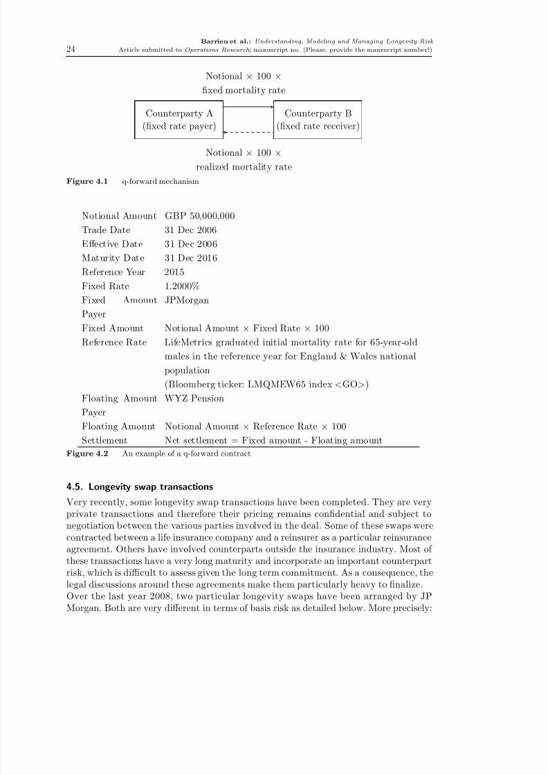
4.4. q-forwards

JP Morgan has been particularly active in trying to establish a benchmark for alongevity market. Not only have they developed the longevity risk platform LifeMetricsbut also some standardized longevity instruments called ”q-forwards”. These contractsare based upon an index, which can either be the mortality rate or the survival rate,as quoted in LifeMetrics. Very naturally, survivor swaps are more intuitive hedginginstruments for pension funds and insurers. But as the survival rate is path-dependentand so the starting date of the contract is important, this may prevent the fungibilityof the different contracts relating to the same cohort and time in the future and there-fore mortality swaps are also likely instruments. The mechanisms of a q-forward canbe summarized as follows:

The mechanisms of the q-forwards are quite simple: a pension fund hedging itslongevity risk will expect to be paid by the counterpart of the forward if the mortalityfalls by more than expected. So typically, a pension fund is a q-forward seller, while aninvestor is a q-forward buyer.




Counterparty A(xed rate payer)

Counterparty B(xed rate receiver)

Notional × 100 ×xed mortality rate

Notional × 100 ×realized mortality rate

Figure 4.1 q-forward mechanism

Notional Amount GBP 50,000,000Trade Date 31 Dec 2006Effective Date 31 Dec 2006Maturity Date 31 Dec 2016

Reference Year 2015Fixed Rate 1.2000%Fixed AmountPayer

JPMorgan

Fixed Amount Notional Amount × Fixed Rate × 100Reference Rate LifeMetrics graduated initial mortality rate for 65-year-old

males in the reference year for England & Wales nationalpopulation(Bloomberg ticker: LMQMEW65 index < GO> )

Floating AmountPayer

WYZ Pension

Floating Amount Notional Amount × Reference Rate × 100Settlement Net settlement = Fixed amount - Floating amount

Figure 4.2 An example of a q-forward contract

4.5. Longevity swap transactions

Very recently, some longevity swap transactions have been completed. They are veryprivate transactions and therefore their pricing remains condential and subject tonegotiation between the various parties involved in the deal. Some of these swaps werecontracted between a life insurance company and a reinsurer as a particular reinsuranceagreement. Others have involved counterparts outside the insurance industry. Most of these transactions have a very long maturity and incorporate an important counterpartrisk, which is difficult to assess given the long term commitment. As a consequence, thelegal discussions around these agreements make them particularly heavy to nalize.Over the last year 2008, two particular longevity swaps have been arranged by JPMorgan. Both are very different in terms of basis risk as detailed below. More precisely:




A customized swap transaction In July 2008, JP Morgan executed a customizedlongevity swap with a UK life insurer for a notional amount of GBP 500 millions for40 years. The life insurer has agreed to pay xed payments and to receive oatingpayments which replicates the actual benet payments made on a closed portfolio of retirement policies. The swap is before all a hedging instrument of cash ows for the

life insurer, with no basis risk.At the same time, JP Morgan entered into smaller swaps with several investors who takethe longevity risk at the end. In this type of indemnity based transaction, the investorsare provided with the relevant information regarding the underlying portfolio as to beable to assess their risk. The back-to-back swap structure of this transaction meansthat JP Morgan has no residual longevity exposure. The longevity risk is transferredfrom the insurer to the investors in return for a risk premium. The counterpart risk forthis swap is important given the long term maturity of the transaction, but also thenumber of agents involved.

A standardized transaction: Lucida In January 2008, JP Morgan executed a stan-dardized longevity swap with the pension insurer Lucida for a notional amount of GBP100 millions for 10 years, and using LifeMetrics index for England and Wales as under-

lying index. This swap structure enables a value hedge for Lucida, which has acceptedin this case to keep the basis risk. For more details on both transactions in particularand on longevity swaps, please refer to Barrieu and Albertini (2009).

Longevity risk is very specic as previously underlined but the market for longevityrisk is also very particular, being strongly unbalanced in terms of exposures and needs.This makes the question of the pricing of risk transfer solutions particularly impor-tant but even before this, the problem of designing suitable, efficient and attractivestructures for both risk bearers and risk takers absolutely essential, as underlined bythe failure of the EIB-BNP Paribas longevity bond in 2005. The recent nancial crisishas also emphasized the importance of assessing counterpart risk, and properly man-aging collateral accounts, which help to secure transactions. These questions are even

more critical when considering longevity risk, due to the long-term maturity of thetransactions, but also the social, political and ethical nature of this risk.

5. Modeling issues for pricingDesigning longevity securities brings together various modeling issues besides the purelongevity risk modeling challenges. Firstly, the pricing of any longevity ”derivative”is not straightforward and it depends on the estimate of uncertain future mortalitytrends and the level of uncertainty. This risk induces a mortality risk premium thatshould be priced by the market. However because of the absence of any liquid tradedlongevity security, it is today impossible to rely on market data for pricing purposes.Long term interest rate should play a key role for the valuation of such derivatives withlong maturities (up to 50 years), creating new challenges in terms of modeling.

5.1. Pricing methodologies

In this section, we investigate methodologies for pricing longevity-linked securities.Note rst that the longevity market is an immature market based on a non-nancialrisk. Therefore, the classical methodology of risk neutral pricing cannot be used care-lessly.




The lack of liquidity of the market induces incompleteness, which is typically the casewhen non-hedgeable and non-tradable claims exist. Thus, to price some nancial con-tracts on longevity risk, the use of a classical arbitrage-free pricing methodology isfar from being applicable as it relies upon the idea of risk replication. The replicationtechnique is only possible for markets with high liquidity and for deeply traded assets.

It induces a unique price of the contingent claim, which is the cost of the replicat-ing portfolio hedging away the market risk. Hence, in a complete market the price of the contingent claim is the expectation of the future discounted cash-ows under theunique risk neutral probability measure. On the contrary, in a longevity-linked securi-ties market, there will be no universal pricing probability measure, and then the choiceof the pricing probability measure is crucial.What will be a good pricing measure for longevity? The historical probability measurewill naturally play a key role because the reliable data we have are given under thisprobability measure. Therefore, it seems natural to look for a pricing probability mea-sure equivalent to this historical probability measure. A relevant pricing measure mustbe robust with respect to the statistical data but also coherent with the prices of the

liquid assets quoted in the market. Therefore, a relevant probability measure shouldmake the link between the historical vision and the market vision. Once the subset of all such probability measures capturing the whole information we wanted is specied,we can look for the optimal one by maximizing the likelihood or the entropic criterion.

5.1.1. Characterization of a pricing rule The question of the pricing rule isalso essential when considering nancial transactions in an incomplete market.

Classical pricing methods The change of probability measures, from the historicalprobability to the pricing one, introduces a longevity risk premium. This method issimilar to those based upon actuarial arguments, where the price of some risky cash-ow F can be obtained as

π(F ) = E P (F ) + λσ P (F ).

The risk premium λ is a measure of the Sharpe ratio of the risky cash-ow F . Differentauthors have studied the impact of the choice of the probability measure on the pricing(Jewson and Brix (2005)) for another type of nancial contracts, namely the weatherderivatives.As recalled before, in a very liquid and complete market where risky derivatives can bereplicated by a self-nancing portfolio, the risk-neutral (universal) pricing rule is used:

π(F ) = E P∗(F ) = E P (F )+cov F,dP∗

dP.

This pricing rule is linear as the actuarial rule does not take into account the riskinduced by large transactions. However, when hedging strategies can not be con-structed, the nominal amount of the transactions becomes an important risk factorand this methodology is not accurate any more, especially when the market is highlyilliquid. To face this problem, the utility based indifference pricing methodology thatwe present below seems to be more appropriate.




Indifference pricing In an incomplete market framework, where a perfect replicationis no longer possible, a more appropriate point of view involves utility maximization.Following Hodges and Neuberger (1989), the maximum price that an agent is ready topay is the price such that she is indifferent (from her preference point of view) betweendoing or not the transaction. More precisely, given a utility function ub and an initial

wealth W b0 , the indifference buyer price of F is π

b

(F ) determined by the non linearrelationship:E P ub(W b0 + F − π b(F ) = E P ub(W b0 ) .

This price, which theoretically depends on the initial wealth and on the utility function,is not necessarily the price at which the transaction will take place. This gives an upperbound to the price the agent is ready to pay. Similarly, the indifference seller price isrelated to the preference of the seller and characterized by

E P us (W s0 − F + π s (F ) = E P us (W s0 ) . (5.1)

We should note that this pricing rule is non-linear and provides a price range (difficultto compute) instead of a single price.

Fair price for small transactions When the agents are aware of their sensitivity tothe unhedgeable risk, they can try to transact for only a little amount in the riskycontract. In this case, the buyer wants to transact at the buyer’s ”fair price”, whichcorresponds to the zero marginal rate of substitution pb.

∂ θ E P ub(W b0 + θF ) |θ=0 = ∂ θ E P ub(W b0 − θp(F )) |θ =0

that implies pb(F ) = E P ubx (W b0 )F / E P ub

x (W b0 ) . (5.2)

The same formula holds when the random initial wealth W b0 is in fact the value of theoptimal portfolio of the classical optimization problem in incomplete market related tothe utility function ub. In this case, the normalized random variable ub

x (W b0 ) may be

viewed as the optimal martingale measure.When both agents have the same utility function, they can transact at this fair price.Therefore, with an exponential utility function, the fair price for a small transaction isequivalent to the one given by the expectation under an equivalent probability measure.This methodology can be compared to the Wang transform, which is a distortion of the historical probability. If we linearise the Wang transform, this also leads to anequivalent change in probability measures.

Economic point of view When adopting an economic point of view, the transactionprice is an equilibrium price, either between the seller and the buyer, or betweendifferent players in the market, where the agents maximize their expected utility atthe same time (Pareto-optimality). Obviously a transaction takes place if it is possibleto nd two agents for whom π b(F ) π s (F ).

5.1.2. A dynamic point of view The economic pricing methodologies describedin the above subsection are static and correspond in this respect mainly to an insuranceor accounting point of view. The standard nancial approach to pricing is howeverdifferent and relies on the so-called risk-neutral methodology. The main underlyingassumption of this approach is the possibility to replicate dynamically the cash owsof a given transaction using the basic traded securities in a market with high liquidity.




Using a non-arbitrage argument, the price of the contract is then uniquely denedas the cost of this replicating strategy. It can also be proved that this cost is in factthe expected value of the discounted future cash ows using a risk neutral probabilitymeasure as reference. This approach is clearly dynamic since the construction of thereplicating strategy is done dynamically. Note that the replicating portfolio is not only atool to nd the price of the contract, but can also be used to hedge dynamically the risksassociated with the transaction. Adopting such an approach for the pricing of nancialcontracts based upon mortality or longevity risks requires therefore a dynamic modelingof the underlying risks (see subsection 5.2). Besides, the cash ow are actualized andlongevity-linked securities have a long maturity, thus this approach raises also somespecic issues related to dynamic long term interest rate (see subsection 5.3). It ishowever important to emphasize the need to have a very liquid underlying market,which is essential for the construction of the replicating strategy. But, as mentionedbefore, as it now stands, the longevity market is far from been liquid and this riskneutral methodology has been questioned in many research papers, such as Bauer et al.(2008). An appropriate point of view may be to extend the fair price approach to anilliquid and dynamic setting : since a perfect hedge does not exist, we can extend ( 5.2)as

sup E P us (W s0 − F + π s (F ) = E P u s (W s0 ) , (5.3)

where π s (F ) is not a static price anymore but a dynamic price strategy associated witha hedge and the supremum in ( 5.3) is taken over the strategies. Thus an optimal hedgegiven criteria ( 5.3) is derived (see Barrieu and El Karoui (2009)).

5.1.3. Design issues Due to the absence of liquidity and maturity of the longevitymarket, a dynamic replicating strategy cannot be constructed and therefore the variousrisks embedded in a longevity transaction will be difficult to hedge dynamically. Asa consequence, investors will not only consider the pricing of a transaction but willalso take into consideration its design to choose the one which seems to be the lessrisky from their own point of view. Therefore, the design of new securities appears asan extremely important feature in the transaction. It may be the difference betweensuccess and failure.The problem is now to design a contract F and a price π(F ) such that both the sellerand the buyer would like to do the transaction. Such a problem has been studied indetails by Barrieu and El Karoui (2009). An interesting feature of the risk transferappears when both agents have the same utility function but different risk tolerance:ub(x) = γ bu(x/γ b) and us (x) = γ s u(x/γ s ). Given an initial risk that the seller wantsto partially transfer to the buyer, the best choice is to transfer F ∗= γ b

γ s + γ b X . Thanksto the optimality of F ∗, it can be shown that there still exists a pricing probabilitymeasure common to both agents, but depending on the pay-out of the derivatives.Nevertheless, this feature is somehow simplistic because investors do not share usuallythe same utility function (because, for example, they do not have access at the samemarket). Thus the issue does not reduce to the transfer mentioned above, but becomesmore crucial and complex.




5.2. Stochastic mortality modeling for nancial transactions

For pricing longevity linked securities, we need to develop future mortality forecastingmodels that are more accurate than those used by insurance companies. Thus, we canenrich the models introduced in Section 2.1 by introducing more uncertainty in theirparameters. As we have seen earlier, in a deterministic approach for the hazard rateµ(x, t ), the survival probability of an individual aged x at time t is dened as:

S t (x, T ) = P t (τ > x + ( T − t) | τ > x )=exp( − T

tµ(x + s − t, s )ds). (5.4)

This can also be extended to a stochastic hazard rate µ(x, t ) using two differentapproaches. First, by analogy with periodic life tables, the period approach modelsthe process s → µ(x, s ) for each age x. In this case, µ(x, s ) is referred to as the spotmortality rate (see Milevsky and Promislow (2001)). On the other hand, by analogywith life tables, the second approach is cohort-based and models instead the processs → µ(x + s, s ), taking into account the whole future mortality evolution.

More precisely, let (Ω , (F t ) t 0 , P ) be a probability space representing the uncertainty

under the historical probability measureP

. The intensity process µ(x, t ) is adapted tothe information F t available to the agents at any time t. The survival probability isnow dened as:

S t (x, T ) = P t τ > x + ( T − t) | τ > x = E t exp( − T

tµ(x + s − t, s )ds) . (5.5)

Here P t (.) stands for the conditional probability of P with respect to F t , and x for theage of the cohort at time t.Using Equation ( 5.5), the hazard rate can be dened as:

µ(x, T ) = − limt ↑ T

∂ T ln S t (x, T )

= limt ↑ T −∂

∂T ln E t (exp( − T

t µ(x + s − t, s )ds)) . (5.6)

Note that µ(x, T ) is indeed µ(xT , T ), where xT is the age of the individual at time T .On the one hand, if we consider a cohort based mortality modeling, we can dene thequantity µt (x, T ) where x is the age at time t by

µt (x, T ) = −∂

∂T ln E t exp( − T

tµ(x + s − t, s )ds . (5.7)

By analogy with interest rates framework or credit risk modeling, µt (x, T ) is calledthe instantaneous forward mortality rate. Note that S t (x, T ) is equivalent here to theprice at time t of a defaultable zero-coupon bond maturing at T . This denition is

very useful when valuing insurance contracts because it takes into account the wholeage-term structure of mortality, which is consistent with insurers practices.On the other hand, in the periodic approach of mortality modeling ( spot mortalityrates), some authors ( Schrager (2006) and Dahl (2004) or Biffis (2005)) introduce theso-called intensity framework to stochastic mortality modeling, which is very popu-lar both in interest rates and credit risk modeling. By doing so, they draw an anal-ogy between death time and the default time. Moreover, this methodology has great




underpins because it facilitates the derivation of closed-form formulae for survival prob-abilities, especially when assuming an affine diffusion for the mortality hazard rateprocess µ(x, t ). However, this class of processes shows restrictive behaviors and donot ensure positive mortality intensities. Gourieroux and Sufana (2003) have outlinedthese drawbacks and introduced a new class of processes: the so-called quadratic class.

Following this approach, Gourieroux and Monfort (2008) use a quadratic stochasticintensity model with a Gaussian autoregressive factor to model spot mortality rates.This proves to be more suitable and consistent with historical data. They also underlinethe tractability of such processes when used to evaluate insurance contracts using a riskneutral approach. Nevertheless, the intensity approach for mortality is more complexthan in credit risk, because the hazard rate depends on the age x and this dependencyis difficult to model and capture in such a framework.Henceforth, it will be essential to understand on which data the various parameters of the models have to be estimate statistically. The most accurate and reliable data weget are the national data of mortality. However, as we have mentioned in Section 2.4,these mortality tables present signicant differences from a country to another and areheterogeneous.

The statistical data will be used to construct pricing methodologies for longevity-linkedsecurities. As for derivatives written on non-nancial risk, in an immature market,there would be no nancial benchmark to estimate the market risk premium.

5.3. Long-term interest rates

Financial contracts written on mortality-related risks typically have a maturity up to20 years, while, on the other hand, longevity-linked securities are typically character-ized by a much longer maturity (40 years and beyond). In most of these contracts,there is an embedded interest rate risk. For the shorter time horizon (up to 20 years),the standard nancial point of view can be used to hedge this risk as the interest ratemarket with such maturities is quite liquid. However, this is not the case anymore forlonger maturities as the interest rate market becomes highly illiquid and the standardnancial point of view cannot be easily extended. Nevertheless, an abundant literatureon the economic aspects of long-term policy-making (i.e. a time horizon between 50 to200 years), has been developed.The economic assumptions set to handle the problem concern, rst of all, the agentpreferences. As for the pricing problem discussed above, the agent is considered to berisk-averse and her utility function on consumption is assumed to be differentiable,increasing and concave. Moreover, she is assumed to behave as a price taker. In thisframework the optimal interest rate for each maturity is derived from an equilibriumlinking together the saving-consumption dilemma to the optimal utility over the givenperiod. This approach is inspired from the well-known neoclassical economical the-ory and has been outlined by many authors (e.g. Gollier (2007, 2008), Hansen andScheinkman (2009) and Breeden (1989)). It focuses on the aggregate behavior of allagents, and the economy is represented by the strategy of the representative agent. Thisis the same economic model introduced by Breeden (1989). The derivation of the yieldcurve for far-distant maturities is induced from the maximization of the representativeagent’s intertemporal utility function on the aggregate consumption :

maxc 0 t 0

e− δt u(ct )dt




where ct is the aggregate consumption, u the agent’s utility function and δ her puretime preference parameter (i.e. δ quanties the agent preference of immediate goodsversus future ones). In the setting of deterministic rate and consumption, the optimalconsumption is given by:

u (

ct )e− δt = u (c0)e− t

0 r s ds

where r t is the spot rate and e− t

0 r s ds the discount factor. This leads to the so-called”Ramsey rule”

1t t

0r s ds = δ −

1t

lnu ( ct )u (c0)

. (5.8)

Adding uncertainty on the interest rate and the consumption, the maximization of therepresentative agent’s utility function takes into account the budget constraint

maxc 0 t 0

e− δt E (u(ct )) dt s.t . E t 0e− t

0 r s ds ct dt x0.

The budget constraint expresses the initial wealth x0 in the economy that allows tonance the consumption plan ct . The optimal consumption is given pathwise by:

E (u ( ct ))e− δt = u (c0)e− t0 r s ds .

The initial consumption c0 is a function of the initial wealth x0 , given by the budgetconstraint. Note that the consumption is deterministic if and only if the interest rateis deterministic. The Ramsey rule can be extended in this stochastic framework :

R0(t) :=1t

ln E e t0 r s ds = δ −

1t

lnE (u ( ct ))

u (c0), (5.9)

Developing this solution using the second-order Taylor approximation leads to thefollowing equation (see Gollier (2007)):

R0(t) δ + R(c0)E

( ct ) − c0tc0

− 12R(c0)P (c0) V ar( ct /c 0)t ,

where R(c) = − cu (c)u (c)

is the relative risk aversion parameter and P (c) = − cu (c)u (c)

is

the relative prudence parameter. The yield curve is now governed by three main behav-iors of the agent facing a consumption-saving problem (i.e. the three terms on righthand side of the equation above). First of all, the representative agent is interested ingoods bringing an immediate satisfaction rather than those with the same effect laterin the future. This effect works in an additive manner with the ”wealth effect”, i.e.the agent prefers to consume rather than to save in sight of potential better days inthe future, which is incorporated in the deterministic trend on growth in the economic

evolution (i.e. consumption). Finally, the ”precautionary effect” appears. It increasesas the future is uncertain and with the representative agent’s willingness to save.For example, Gollier (2007, 2008) studies the case of a consumption given by a geo-metric Brownian motion and Hansen and Scheinkman (2009) uses a pure Levy pro-cess to model the consumption and derive the optimal interest rates yield curve ina Markov environment. Nevertheless, in the economic literature on long-term policy-making, modeling processes in a dynamic way is not common and the usual approach




is deterministic with static random perturbations. Furthermore, the global approachwith a representative agent never takes into account the existence of a market. Tostudy nancial problems involving long term interest rates, we need to look at thisapproach by putting also the nancial market at the heart of our preoccupations.A rst way to achieve this in the case of a liquid market is to consider an agent, who

optimizes the utility of her consumption under the budget constraint. The budget con-straint evaluate the present value of the future cash ows under the pricing probabilityP ∗ (and not under the historical probability P as it was done before) :

maxc 0 t 0

e− δt E (u(ct )) dt s.t . E ∗ t 0e− t

0 r s ds ct dt x0 .

Denoting by L∗

t the density of P ∗ with respect to P , we have

exp(− δt)u ( ct ) = u (c0)exp − t

0r s ds L∗

t .

Thus

B (0, t )=exp( − δt)E [u (

ct )]

u (c∗0) ,

where B (0, t ) = E ∗ exp − t0 r s ds is the price at time 0 of a zero-coupon with matu-

rity t. Therefore, the same relation as (Equation 5.9) - with B (0, t ) = exp( − R0(t)t) -is obtained from a nancial point of view, in the case of a liquid market. In the caseof an illiquid market, the pricing probability is not universal and might depend on thematurity and the utility function. Thus the budget constraint takes a more complexform. The consequences on Equation ( 5.9) are an important issue we are currentlyworking on.This model can be enriched by considering a stochastic utility function : the case wherethe agent preferences are unknown is treated by Lazrak and Zapatero (2004) using

a stochastic utility function modeling the fact that the agent can change her beliefsduring the considered period.

6. ConclusionHaving presented its main characteristics and the state of the art in its understandingand modeling, longevity risk appears to be a very complex risk, due to its specicitiescompared with other insurance risks - in particular the trend sensitivity, the geograph-ical variability and the associated long-term maturities - and its potential correlationswith other sources of risk, nancial and non-nancial.As a recent move, the insurance industry and especially the life insurance sector areadopting new regulations not only to allow for a more accurate risk assessment but also

to impose more effective solvency risk management rules. Those regulations and theincreasing convergence between insurance and capital markets have opened the wayfor alternative risk management solutions and innovative risk transfers. To supportthe emergence of this new market, not only any asymmetry of information betweenthe various agents involved in potential transactions has to be reduced but it is alsonecessary to develop specic pricing methods and partial hedging methodologies, well-suited to the particular features of longevity risk and to the immature and illiquid




state of the current market. Additional challenges appear naturally, especially relatedto the modeling of long term interest rate due to the long maturities of the potentialtransactions.However, the longevity risk is far from being a concern for the insurance industry alone.It is indeed at the core of an open discussion for politicians, economists and strate-

gists, who have to determine the ”effective” retirement age and the ”effective” pensionscheme as the future generations will almost surely face one of the greatest challengeswith an increasing life expectancy. The potential impacts of longevity risk at variouslevels of the global economy and society make a better management of this risk one of the key challenges of the coming decade. Interactions with other sources of risk, suchas dependence, economy, or ecology, have not been investigated in-depth in this paper.But it would be certainly very interesting to study at a macro-level the impacts of longevity on the whole economy and the environment.

ReferencesAntolin, P., H. Blommestein. 2007. Governments and the market for longevity-indexed bonds.

OECD Journal : Financial Market Trends .Barrieu, P., L. Albertini. 2009. The handbook of insurance-linked securities . Wiley Finance.Barrieu, P., N. El Karoui. 2009. Pricing, hedging and optimally designing derivatives via min-

imization of risk measures. R. Carmona, ed., Volume on Indifference Pricing . PrincetonUniversity Press, 77–146.

Bauer, D., Boerger M., J. Russ. 2008. On the Pricing of Longevity-Linked Securities. Tech.rep., Working Paper. Available at: www.mortalityrisk.org.

Bensusan, H., N. El Karoui. 2009. Microscopic modelling of population dynamic : An analysisof longevity risk. Preprint .

Bienvenue, A., A. Illig, L. Loisel, D. Serant. 2009. On inter-age correlations in stochasticmortality models. Working Paper .

Biffis, E. 2005. Affine processes for dynamic mortality and actuarial valuations. InsuranceMathematics and Economics 37 (3) 443–468.

Breeden, D.T. 1989. An intertemporal asset pricing model with stochastic consumption andinvestment opportunities. Theory of Valuation: Frontiers of Modern Financial Theory 753.

Cairns, A.J.G., D. Blake, K. Dowd. 2006. A two-factor model for stochastic mortality withparameter uncertainty: Theory and calibration. Journal of Risk & Insurance 73 (4) 687–718.

Cairns, A.J.G., D. Blake, K. Dowd. 2008. Modelling and management of mortality risk: areview. Scandinavian Actuarial Journal 108 (2) 79–113.

Cairns, A.J.G., D. Blake, K. Dowd, G.D. Coughlan, D. Epstein, A. Ong, I. Balevich. 2007. Aquantitative comparison of stochastic mortality models using data from England & Walesand the United States. Working paper, Heriot-Watt University, and Pension InstituteDiscussion Paper PI-0701 .

Cambois, E., Laborde C., J.M Robine. 2008. La ”double peine” des ouvriers : plus d’anneesd’incapacite au sein d’une vie plus courte. Population et Societes (441).

Ceiops. 2008. Quantitative impact study. Tech. rep., European Commission, available at:http://www.ceiops.eu/content/view/118/124/ .

http://www.ceiops.eu/content/view/118/124/






Cox, S.H., Y. Lin, A. Milidonis. 2009. Mortality Regimes and Pricing. Tech. rep.Currie, I.D., M. Durban, P.H.C. Eilers. 2004. Smoothing and forecasting mortality rates. Sta-

tistical Modelling 4(4) 279.Dahl, M. 2004. Stochastic mortality in life insurance: market reserves and mortality-linked

insurance contracts. Insurance Mathematics and Economics 35 (1) 113–136.

Denuit, M., A. Delwaerde. 2005. Construction de tables de mortalite periodiques et prospectives .Economica.

El Karoui, N., S. Loisel, C. Mazza, A. Shirayev. 2009. Detection of changes in longevity trendsby banks, insurers and reinsurers. Working Paper .

FAP. 2007. Personnes ˆagees et medicaments. Activity report, available at: http: // www.acadpharm. org/medias/ direct/ Agees. pdf .

Fournier, N., S. Meleard. 2004. A microscopic probabilistic description of a locally regulatedpopulation and macroscopic approximations. Annals of Applied Probability 1880–1919.

Gavrilov, L.A., N.S. Gavrilova. 2001. The reliability theory of aging and longevity. J. Theoret.Biol. 213 (4) 527–545.

Gollier, C. 2007. The consumption-based determinants of the term structure of discount rates.

Mathematics and Financial Economics 1(2) 81–101.Gollier, C. 2008. Discounting with fat-tailed economic growth. Journal of Risk and Uncertainty

1–16.Goshay, R.C., R. Sandor. 1973. An inquiry into the feasibility of a reinsurance futures market.

Journal of Business Finance 5(2) 56–66.Gourieroux, C., A. Monfort. 2008. Quadratic stochastic intensity and prospective mortality

tables. Insurance Mathematics and Economics .Gourieroux, C., R. Sufana. 2003. Wishart quadratic term structure models. Tech. rep., working

paper, University of Toronto.Hansen, L.P., J.A. Scheinkman. 2009. Long-term risk: An operator approach. Econometrica

77 (1) 177–234.Hodges, S.D., A. Neuberger. 1989. Optimal replication of contingent claims under transaction

costs. Review of futures markets 8(2) 222–239.Jewson, S., A. Brix. 2005. Weather derivative valuation: the meteorological, statistical, nancial

and mathematical foundations . Cambridge University Press.Jusot, F. 2004. Mortalite, revenu et inegalites de revenu en france : une analyse multi-niveaux.

IRDES .Kirkby, J., I. Currie. 2007. Smooth models of mortality with period shocks. Age 20 (40) 60.Klein, J.P., M.L. Moeschberger. 2003. Survival analysis: techniques for censored and truncated

data . Springer.Lazar, D., M. Denuit. 2009. A multivariate time series approach to projected life tables. Working

Paper .Lazrak, A., F. Zapatero. 2004. Efficient consumption set under recursive utility and unknown

beliefs. Journal of Mathematical Economics 40 (1-2) 207–226.Lee, R. D., L. Carter. 1992. Modelling and forecasting the time series of us mortality. Journal

of the American Statistical Association 87 659–671.Milevsky, M.A., S.D. Promislow. 2001. Mortality derivatives and the option to annuitise. Insur-

ance Math. Econom. 29 (3) 299–318. 4th IME Conference (Barcelona, 2000).Monnier, A. 2000. La population de l’Europe : 1950-2050. Population et Societes (353).

http://www.acadpharm.org/medias/direct/Agees.pdf







Pitacco, E. 2004. Survival models in a dynamic context: a survey. Insurance Mathematics and Economics 35 (2) 279–298.

Renshaw, A.E., S. Haberman. 2003. On the forecasting of mortality reduction factors. InsuranceMathematics and Economics 32 (3) 379–401.

Renshaw, A.E., S. Haberman. 2006. A cohort-based extension to the Lee–Carter model for

mortality reduction factors. Insurance Mathematics and Economics 38 (3) 556–570.Salhi, Y., S. Loisel, M. Denuit. 2009. Joint modeling of portfolio experienced and national

mortality: A co-integration based approach. Working Paper .Schrager, D.F. 2006. Affine stochastic mortality. Insurance Mathematics and Economics 38 (1)

81–97.Tran, V.C. 2006. Modeles particulaires stochastiques pour des problemes d’evolution adaptative

et pour l’approximation de solutions statistiques. Ph.D. Thesis .Tran, V.C. 2007. Large population limit and time behaviour of a stochastic particle model

describing an age-structured population. ESAIM .Tran, V.C., S. Meleard. 2009. Age structured trait substitution sequence process and canonical

equation. Journal of Mathematical Biology .

Webb, G.F. 1985. Theory of nonlinear age-dependent population dynamics . Marcel Dekker.

understanding modeling and managing longevity risk

Documents