understanding the effects of model uncertainty in robust...
TRANSCRIPT
Daniel W. Apley1
Associate Professor
Jun LiuGraduate Student
Department of Industrial Engineering andManagement Sciences,
Northwestern University,Evanston, IL, 60208-3119
Wei ChenAssociate Professor
Department of Mechanical Engineering,Northwestern University,
Evanston, IL, 60208-3111
Understanding the Effects ofModel Uncertainty in RobustDesign With ComputerExperimentsThe use of computer experiments and surrogate approximations (metamodels) introducesa source of uncertainty in simulation-based design that we term model interpolationuncertainty. Most existing approaches for treating interpolation uncertainty in computerexperiments have been developed for deterministic optimization and are not applicable todesign under uncertainty in which randomness is present in noise and/or design vari-ables. Because the random noise and/or design variables are also inputs to the meta-model, the effects of metamodel interpolation uncertainty are not nearly as transparent asin deterministic optimization. In this work, a methodology is developed within a Bayesianframework for quantifying the impact of interpolation uncertainty on the robust designobjective, under consideration of uncertain noise variables. By viewing the true responsesurface as a realization of a random process, as is common in kriging and other Bayesiananalyses of computer experiments, we derive a closed-form analytical expression for aBayesian prediction interval on the robust design objective function. This provides asimple, intuitively appealing tool for distinguishing the best design alternative and con-ducting more efficient computer experiments. We illustrate the proposed methodologywith two robust design examples—a simple container design and an automotive enginepiston design with more nonlinear response behavior and mixed continuous-discrete de-sign variables. �DOI: 10.1115/1.2204974�
Keywords: model uncertainty, interpolation uncertainty, metamodel, robust design,Bayesian prediction interval, computer experiments
1 IntroductionSimulation-based engineering analyses �e.g., finite element
analysis �FEA�, computational fluid dynamics� are increasinglyimportant tools for product design �1–3�. This is particularly truewhen the need to reduce product development time and cost ne-cessitates early-stage simulation analyses before actual productionor prototype experimentation is possible. On a parallel front, withincreasing expectations for high quality, reliable, low cost prod-ucts, the issue of robust product design under uncertainty contin-ues to grow in importance �4–15�. In robust design, key systemresponse variables are viewed as functions of a set of design vari-ables �or “control” variables� specified as part of the decisionmaking in product design and a set of uncontrollable “noise” vari-ables that involve uncertainty. If we assign probability distribu-tions to the noise variables, then the response variables are alsoviewed as probabilistic. Broadly speaking, the robust design ob-jective is to select the design variables in order to optimize certainprobabilistic characteristics of the objective responses �typicallyinvolving the mean � and standard deviation � of each response��16�, while ensuring that the constraint responses satisfy certainconditions with some desired probability �6,17–20�.
In the simulation arena, increases in computing power are oftenoffset by increased accuracy �e.g., finer mesh sizes in FEA� andincreased simulation scope/complexity �e.g., multidisciplinarysimulation�, so that computational expense remains a barrier. Forexample, finite-element based automotive structural simulations toassess crash worthiness may take days to execute a single run
1Corresponding author.Contributed by the Design Automation Committee of ASME for publication in the
JOURNAL OF MECHANICAL DESIGN. Manuscript received September 16, 2005; final
manuscript received December 19, 2005. Review conducted by Shapour Azarm.Journal of Mechanical Design Copyright © 20
�21�. The inevitable result is that it generally becomes impossibleto conduct enough simulation runs to thoroughly cover the entireinput variable space and provide a globally accurate understand-ing of the functional relationship between the response and theinputs. We must instead attempt to optimize the design based onthe output of simulation runs conducted at only a limited numberof input variable combinations �also known as sampling sites�.
A common strategy in this situation is to fit some form of sur-rogate model �also called “metamodel” �22�� to the samples and torely on that for optimization purposes. Comprehensive reviews ofmetamodeling applications in mechanical and aerospace systemscan be found in Refs. �23–25�. Typical choices for metamodelstructure are polynomial functions �26�, kriging models �27,28�,and radial basis function networks �29,30�. Examples of recentstudies on enhancing metamodeling techniques for engineeringdesign applications include the work from Refs. �31–40�. Al-though the majority of prior work on metamodel-based design isfor deterministic optimization, a number of researchers �21,41,42�have used fitted metamodels for robust design optimization withnoise variables.
The obvious drawback of simply using a fitted metamodel tooptimize the design is that it may be quite far from the true re-sponse surface. In essence, it ignores metamodel uncertainty, i.e.,the uncertainty that results from not knowing the output of thecomputer simulation code, except at a finite set of sampling sites.Kennedy and O’Hagan �43� referred to this type of uncertainty ascode uncertainty. We adopt the term interpolation uncertainty,because we believe it is more descriptive: The uncertainty disap-pears precisely at the sampling sites because the simulation codeis repeatable, and the uncertainty grows as we stray further fromthe sampling sites and attempt to interpolate the response between
sampling sites using some appropriately fitted metamodel.JULY 2006, Vol. 128 / 94506 by ASME

Widespread efforts have been made in the statistical communityto quantify interpolation uncertainty in computer experiments�28,43,44�. In one of the most popular approaches, the responsesurface is viewed as a realization of a Gaussian random process�GRP�, and Bayesian methods are used to interpolate/extrapolatethe response surface by calculating its posterior distribution giventhe sampling sites. This provides a direct means of representingthe effects of interpolation uncertainty in deterministic optimiza-tion problems, in which the objective function is simply the outputresponse of the computer simulation. Bayesian analyses withGRPs have been used in deterministic optimization to developsequential sampling strategies for the purposes of either efficientlyarriving at the optimum �45,46� or capturing local irregularities inthe global response behavior �39,40�.
Although Jin et al. �47� have argued that metamodel inaccuracyhas an even larger effect in robust design optimization than indeterministic optimization, very few existing approaches for treat-ing interpolation uncertainty in computer experiments apply in theformer situation. The reason is that in robust design optimization,the effects of interpolation uncertainty on the objective functionare not nearly as transparent as in deterministic optimization, be-cause some of the metamodel inputs are random �the noise vari-ables�. Consider a robust design objective function that is aweighted combination c1�+c2� of the response mean and stan-dard deviation �or equivalently, �+c� with weighting constant c=c2 /c1�, which might be appropriate if the design objective was tomake the response as small as possible �“smaller-the-better”� un-der consideration of the uncertainty in the noise variables. Themean � and variance �2 of the response must be obtained byintegrating the uncertain response surface over the full range ofvalues of the noise variables. Moreover, unlike in deterministicoptimization, we cannot eliminate the effects of interpolation un-certainty with validation runs in robust design optimization, be-cause this would require a large number of simulations coveringthe full range of values for the noise variables at the selecteddesign sites. Due to these difficulties, existing metamodel-baseddesign approaches are either for deterministic optimization prob-lems or, in the case of robust design optimization with noise vari-ables, they simply rely on a fitted global metamodel while ignor-ing interpolation uncertainty.
The aforementioned difficulties pose a number of challengesand research issues. The fundamental question is how should wequantify the effects of interpolation uncertainty on the robust de-sign objective function with uncertain noise variables, and subse-quently, how can we use this information for design decision mak-ing, e.g., to distinguish the best design alternative. Because thecomputer experiment drives the accuracy of a metamodel, anotherfundamental question is how the quantification of interpolationuncertainty can be used to guide the computer experiment in de-termining whether or not additional samples are needed and, if so,how to select the additional sampling site�s�? A final issue is thepotential computational challenges of the proposed method, espe-cially in problems involving a large number of design and noisevariables.
To address these issues, in this work we develop an approachusing Bayesian prediction intervals �PIs� for quantifying the ef-fects of interpolation uncertainty on the objective function in ro-bust design. To better illustrate the concepts and introduce theproposed methods, a running design example �described in Sec. 2�is used throughout the paper. A brief background on Bayesiananalysis of GRPs is presented next �Sec. 3�. In Sec. 4 we deriveclosed-form analytical expressions for the prediction intervals onthe response mean, the response variance, and the robust designobjective function. The prediction intervals are useful in manycontexts, for example to evaluate a candidate design or comparetwo or more candidate designs. Based on the prediction intervals,in Sec. 5 we provide a method for deciding whether to terminateor continue simulation. The stopping criterion is objective ori-
ented and is intended to terminate when further simulation will946 / Vol. 128, JULY 2006
not lead to a significantly better design. In Sec. 6 we discusssimple graphical methods for guiding the selection of additionalsampling sites. An automotive engine piston design problem ispresented in Sec. 7 to illustrate the applicability of our method forproblems with nonlinear function behavior and mixed continuous-discrete design variables. In Sec. 8 we discuss the handling ofvarious computational issues. Conclusions are summarized in Sec.9.
2 An Illustrative Design ExampleConsider the following simple design optimization example
from Ref. �48�, in which the task is to design an open box that willbe used to ferry a specified quantity of gravel across a river. Thedesign objective is to minimize the total cost y�d ,W�=80d−2
+2dW+d2W �refer to Ref. �48� for details�, where the first term isthe cost of ferrying, the remaining two terms are the total materialcost, and the variables are as follows. The noise variable W rep-resents the material cost per unit, and the design variable d repre-sents the length and width of the square box. In order to representthe material cost uncertainty, we assign to W a normal probabilitydistribution W�N��w ,�w
2 � with mean �w=10 $ /m2 and variance�w
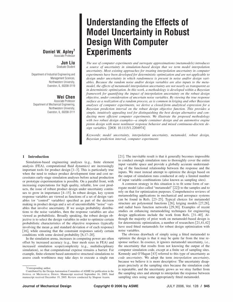
2 =2 $2/m4. The response is plotted in Fig. 1�a�.We cannot minimize cost directly, because of the uncertainty in
W. As a robust design objective �robust with respect to uncertaintyin W�, we will instead minimize the objective function f�d����d�+c��d�, where ��d� and ��d� represent the mean and stan-dard deviation of the response �total cost� with respect to varia-tions in W. Suppose we choose c=3 as our desired relativeweighting of � and � �choice of c is discussed in Sec. 4�. If thetrue response surface in Fig. 1�a� were known, this would be arather trivial design problem. Imagine that instead of having theanalytical expression for y�d ,w�, however, we must rely on acomputationally expensive simulation to evaluate the responseand a fitted metamodel to optimize the design. Fig. 1�b� shows thesimulation output at four sampling sites, as well as one particularfitted metamodel �the details of which are discussed in the follow-ing section� denoted by y�d ,w�. If we ignored interpolation uncer-tainty and treated the fitted model as the true response surface, wecould calculate the response mean and variance as a function of dvia
��d� =� y�d,w�pw�w�dw , �1�
and
�2�d� =� �y�d,w� − ��d��2pw�w�dw �2�
for use in the objective function ��d�+3��d�. Here, pw�w� de-notes the probability density function of w. Figure 1�d� shows��d�, ��d�, and f�d� calculated from Eqs. �1� and �2�, and Fig.1�c� shows the corresponding values calculated by substituting thetrue response surface for y�d ,w� in Eqs. �1� and �2�.
Ignoring metamodel uncertainty clearly has a large effect on thedesign optimization. From Fig. 1�d�, the optimal design thatwould result from assuming that the true response surface coin-cides with y�d ,w� is d=0.8 �we have defined the feasible designspace as 0.8�d�2.5�. In contrast, the optimal design that wouldresult if we knew the true response surface is d=1.3 �see Fig.1�c��. In the subsequent sections, we propose a method for quan-tifying the effects of interpolation uncertainty on the robust designobjective function f , to help designers avoid selecting a designthat is far from optimal because of insufficient computer simula-
tion and the resulting interpolation uncertainty.Transactions of the ASME
l y
3 Review of Gaussian Random Processes and TheirBayesian Analysis
We provide a brief review of Bayesian analysis of GRPs forrepresenting computer simulation response surfaces in this sec-tion. More comprehensive discussions can be found in Refs.�28,43,44,49�. Let the vectors d= �d1 ,d2 , . . . ,dqd
�T and w= �w1 ,w2 , . . . ,wqw
�T denote the sets of design and noise variables,and let y�x� be a scalar response variable, where x= �dT ,wT�T
denotes the vector of inputs. Suppose we run a computer simula-tion at a set of N separate input sampling sites SN
= �s1 ,s2 , . . . ,sN to obtain a vector of N responses yN
= �y�s1� ,y�s2� , . . . ,y�sN��T. Figures 1�a� and 1�b� show the re-sponse at N=4 sampling sites. Given the observed values yN, twonatural questions are how can we predict �in this case, interpolate/extrapolate� the response as we move away from the specific sam-pling sites in SN, and how can we reasonably quantify the predic-tion �interpolation� uncertainty?
Bayesian analysis of GRPs, which one might view as a gener-alization of the kriging method that was popularized in the field ofgeostatistics �50�, is the most widely investigated method for these
Fig. 1 „a… True response surface „treated as unknosampling sites. „b… Fitted surrogate model y based onand robust design objective function f calculated fromand objective function calculated from the fitted mode
purposes. The basic idea is to view the actual response surface
Journal of Mechanical Design
y�x� as a realization of a Gaussian random process G�x� with priormean function E�G�x��=hT�x�� and prior covariance functionCov�G�x� ,G�x���=�2R��x ,x�� �these are intended to be prior toactually running the computer simulation�. Here, �= ��1 ,�2 , . . . ,�k�T is a vector of unknown parameters, hT�x�= �h1�x� ,h2�x� , . . . ,hk�x��T is a vector of known functions of x�e.g., linear or quadratic�, �2 is the variance of G�·�, and for anytwo input vectors x and x�, R��x ,x�� is the correlation coefficientbetween G�x� and G�x��, parameterized in terms of a vector � ofparameters. One of the most common choices for correlation func-tion is
R��x,x�� = i=1
q
exp�− �i�xi − xi��2� �3�
where q=qd+qw. Because � determines the rate at which thecorrelation between G�x� and G�x�� decays as x and x� movefurther apart, � and � relate to the smoothness of the responsesurface and the extent to which it might differ from a parametricsurface of the form hT�x��. A noninformative prior distribution is
2
…, the four bullets indicate simulation output at fourfour sampling sites „c… Mean �, standard deviation �,true response surface. „d… Mean, standard deviation,
.
wnthethe
ˆ
often assigned to �. Although we may view � and � as hyper-
JULY 2006, Vol. 128 / 947

parameters and assign to them a prior distribution as well, it ismore common �for computational purposes� to estimate themfrom the data and then simply view the estimates as given values.We discuss this in Sec. 8�a�.
For notational purposes, let Y�·� denote the response surfacey�·� when viewed as a realization of the random process and writeY�G ,d ,W�=G�d ,W�=G�x�. This allows us to express the re-sponse Y�·� as a function of the design d and two sources ofuncertainty—the noise W and the interpolation uncertainty repre-sented by G�·�. The random process G�·�, together with a priormean and covariance function and a prior distribution for �, areused to represent our prior uncertainty in the response surfaceY�·�. Given the observed values yN, it is quite straightforward touse Bayesian methods to calculate the posterior distribution ofG�·�. The posterior distribution of G�·� provides a direct quantifi-cation of the effects of interpolation uncertainty on the predictedresponse. For a noninformative prior on �, the posterior distribu-tion is Gaussian with posterior mean and covariance given by�27,51�
y�x� � EG�w,yN�Y�G,d,w��w,yN� = hT�x�� + rT�x�R−1�yN − H�� ,
�4�
and
Cov�Y�G,d,w�,Y�G,d�,w���yN�
� EG�w,w�yN��Y�G,d,w� − ��d,w�yN���Y�G,d�,w��
− ��d�,w��yN���w,w�,yN
= �2�R��x,x�� − rT�x�R−1r�x�� + �h�x�
− HTR−1r�x��T�HTR−1H�−1�h�x�� − HTR−1r�x��� �5�
where H is an N�k matrix whose ith row is hT�si�, R is an N�N matrix whose ith row, jth column element is R��si ,sj�, r�x� is
an N�1 vector whose ith element is R��x ,sj�, and �= �HTR−1H�−1HTR−1yN is the posterior mean of �. The subscriptson the expectation operator EG �w ,yN�·� indicate that the expecta-tion is with respect to the posterior distribution of G�·� given W=w and yN. Note that conditioning the expectation on W treats itas a fixed quantity. The preceding results, as well as the vastmajority of the literature on Bayesian analysis of computer experi-ments, have only considered deterministic inputs x. The distinc-tion that we will make in subsequent sections between the deter-ministic d and the random W that characterizes robust designproblems is a nontrivial one.
The usual interpretation of Eqs. �4� and �5� is the following: Forany site x in the input space, y�x� is the best prediction of theresponse Y�x� at that site, and the prediction error variance isgiven by Eq. �5� with x�=x. We may view y�x� as the fittedsurface. One can easily verify that for any sampling site si
= �diT ,wi
T�T at which we have already run a simulation, the predic-tion reduces to y�si�=y�si� and the prediction error variance iszero, as we would desire with perfectly repeatable computer ex-periments.
The reasons why GRPs and Bayesian analyses are so popularfor representing and analyzing computer experiment response sur-faces becomes apparent when one considers three fundamentalcriteria that any metamodel should possess: �i� It should be con-venient to work with, allowing tractable analyses. �ii� The struc-ture of the fitted surface y�x� should be sufficiently versatile torepresent a wide variety of true response surfaces. �iii� It shouldprovide an inherent mechanism for quantitatively assessing theinterpolation uncertainty in the fitted surface. The GRP approachsatisfies all three criteria. The flexibility of the structure of y�x� inEq. �4� stems in part from the generality of the h�x� term. As
pointed out in Ref. �28,44�, many of the most common model948 / Vol. 128, JULY 2006
structures used in metamodeling and approximation theory can beviewed as special cases of the Bayesian approach, depending onthe choice for h�x� and r�x�. These include polynomial functions�26�, kriging models �27,28�, and radial basis function networks�29,30�.
If the form of the fitted metamodel y�x� ends up resembling therather familiar polynomial or radial basis function models, onemight question why it is couched in the more abstract language ofGRPs. The reason relates to the third criterion of quantitativelyassessing the interpolation uncertainty. Standard statistical meth-ods for assessing uncertainty in models fitted to random experi-mental data �see, e.g., Ref. �52�� are inapplicable with computerexperiments, because all of the common estimates of the varianceof the model prediction error are meaningless if the response isperfectly repeatable, as is the case with computer experiments.
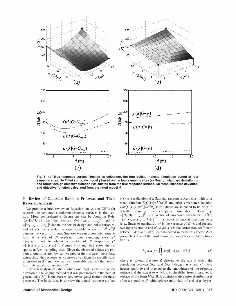
The GRP approach, on the other hand, is ideally suited for thissituation. The random process G should be viewed primarily as ameans of representing our prior knowledge of what we mightexpect the response surface to look like, before any simulationsare run. When this prior knowledge is integrated with the ob-served response values at the sampling sites within the context ofa Bayesian analysis, it dictates our posterior expectations of whatthe response surface might look like between sampled sites. Toillustrate, we continue the container design example by calculat-ing the posterior mean and covariance from Eqs. �4� and �5� basedon the four design sites shown in Fig. 1�b� using prior parameters�= ��d ,�w�= �2,0.1� and �=35, h�x�= �1,d ,w ,dw�T, and a non-informative prior for � �Sec. 8.1 discusses estimation of the priorparameters�. The posterior mean y�d ,w� is that shown in Fig. 1�b�.A number of different GRP realizations were generated from thisposterior distribution, of which three representative realizations�call them G1, G2, and G3� are plotted in Figs. 2�a�–2�c�. Refer toSec. 8.2 for details on how each GRP realization is generated.
Each of the three different GRP realizations reflect what wemight expect the complete true response surface to look like,based on only the four sampling sites and our limited prior knowl-edge. If one were to generate and plot a large number of GRPrealizations, instead of just the three shown in Figs. 2�a�–2�c�, thedifferences between them would directly reflect interpolation un-certainty. Specifically, if we consider a fixed point �d ,w� in theinput space and look at the response y�d ,w� evaluated at that pointfor each GRP realization, the mean and variance of the set ofresponse values would be given by Eqs. �4� and �5�. It is in thissense that the GRP approach allows us to quantify the effects ofinterpolation uncertainty.
4 Derivation of Prediction Intervals for the ResponseMean and Variance and the Objective Function
In this section, we derive a form of Bayesian PI for the meanand variance of the response, which we propose as a direct mea-sure of the impact of interpolation uncertainty on the responsemean and variance. This will lead to a PI on the robust designobjective function for objective functions that are a weightedcombination of the response mean and standard deviation as inEq. �8� below. Hypothetically, if we had a complete response sur-face G�x� available, then in analogy with Eqs. �1� and �2� wecould calculate the response mean and variance �with respect tovariations in the noise variables W over their joint distributionpw�·�� directly via
��d�G� � EW�G�Y�G,d,W��G� �� G�d,w�pw�w�dw , �6�
and
Transactions of the ASME
Fig. 2 „a…–„c… Three realizations of the posterior Gaussian random process G, each of which represents apotential response surface consistent with the four simulated output in Fig. 1„b…. „d…–„f… Mean, standard devia-tion, and objective function calculated from the potential response surfaces in „a…–„c…. Prior parameters:†� ,� ‡= †2,0.1‡ and �=35.
d wJournal of Mechanical Design JULY 2006, Vol. 128 / 949

�2�d�G� � EW�G��Y�G,d,W� − ��d�G��2�G
�� �G�d,w� − ��d�G��2pw�w�dw �7�
The notation throughout will be that p�·� denotes a probabilitydensity, and subscripts indicate which random quantity the distri-bution is with respect to and/or conditioned on. Note that thequantities plotted in Fig. 1�c� are ��d �G=Gtrue� and ��d �G=Gtrue�, where Gtrue denotes the unknown true response surface,and the corresponding quantities in Fig. 1�d� are ��d �G= y� and��d �G= y�.
For the remainder of the paper, the robust design objective thatwe consider is to minimize the objective function
f�d�G� � ��d�G� + c��d�G� �8�
for some specified constant c �e.g., c=3�. For simplicity, we con-sider unconstrained optimization. The approach can be readily ex-tended to the more practical constrained optimization scenario aswe briefly discuss in Sec. 9. The objective function �8� assumesthat we would like the response to be as small a possible �in someprobabilistic sense�. For situations in which we would like theresponse to be as large as possible, we could instead attempt tomaximize an objective function of the form ��d �G�−c��d �G�.The treatment would be similar to what we describe in thissection.
We might view the minimization of �8� as simply attempting toensure that both the mean and the standard deviation of the re-sponse are small. Alternatively, we might view ��d �G�+c��d �G� as an approximate probabilistic upper bound on theresponse. For example, if the response is approximately normallydistributed, then the probability that Y�G ,d ,W� �G���d �G�+c��d �G� is controlled by choice of c �c=3 translates to a prob-ability of 0.9987�. Minimizing �8� therefore corresponds to mini-mizing the worst-case value for �i.e., a probabilistic upper boundon� the response under consideration of the uncertainty in W.Regardless of which viewpoint one takes, the choice of c shouldreflect the designer’s risk aversion. A choice of c=0 representscomplete risk neutrality, because this would result in simply mini-mizing the response mean ��d �G� with complete disregard of theresponse variance. A large c represents high risk aversion. Formany design problems the “optimal” design will obviously de-pend strongly on the desired level of risk aversion.
Of course, we cannot substitute G=Gtrue into Eqs. �6�–�8� tocalculate ��d �G=Gtrue�, ��d �G=Gtrue�, nor the objective functionf�d �G=Gtrue�, because we do not have the complete response sur-face Gtrue. Instead, we propose to use prediction intervals for thesequantities in order to guide the design process. The Bayesian PIapproach involves viewing the quantities ��d �G�, ��d �G�, andf�d �G� as random, being functions of the random surface G. Be-cause the �posterior� distribution of G is used to represent inter-polation uncertainty, the resulting �posterior� distribution off�d �G�, for example, represents the effects of interpolation uncer-tainty on the objective function. This is illustrated in Fig. 2, thebottom panels of which show ��d �G�, ��d �G�, and f�d �G� for thethree realizations of the random G shown in the top panels. Thequantities differ randomly between the three figures, because theyare obtained by integrating the random surface G. Note that��d �G�, ��d �G�, and f�d �G� are random because of their func-tional dependence on G and not because of any dependence on W.The random effects of W have already been averaged out via theintegration in Eqs. �6� and �7�.
This suggests a straightforward approach for quantifying theeffects of interpolation uncertainty on ��d �G�, ��d �G�, andf�d �G�: Calculate their posterior distributions �or approximateposterior distributions� by considering the posterior distribution of
G, similar to the treatment in �53,54�. Based on this, we can then950 / Vol. 128, JULY 2006
calculate PIs �similar to confidence intervals� for the quantities.Rather than producing a single point estimate of the unknownobjective function f�d �G� �which could be quite inaccurate be-cause of interpolation uncertainty�, the PI approach produces arange of possible values that takes into account the level of inter-polation uncertainty.
In order to derive the PI, first consider the posterior distributionof ��d �G�. The integral in Eq. �6� can be viewed as a lineartransformation of the Gaussian random process G. Consequently,��d �G� is exactly Gaussian. Its posterior distribution is thereforedetermined by its mean and standard deviation, which we denoteby ���d� and ���d�. Using Eq. �6� and basic results on the meanand variance of linear transformations of random processes �55�,we have �see Ref. �53� also�
���d� = EG�yN���d�G��yN� = EG�yN�� G�d,w�pw�w�dw�yN =� EG�yN�G�d,w��yN�pw�w�dw
=� y�d,w�pw�w�dw �9�
��2 �d� = EG�yN����d�G� − ���d��2�yN
=�� Cov�Y�G,d,w�,Y�G,d,w���yN�pw�w�dwpw�w��dw�
�10�
where y�d ,w� and Cov�Y�G ,d ,w� ,Y�G ,d ,w�� �yN� are given byEqs. �4� and �5�. In the Appendix we show that a closed-formanalytical expression for ���d� and ���d� can be obtained fromEqs. �9� and �10� for many common choices of h�x� and r�x�. If zp
denotes the 1− p percentile of the standard normal distribution,then a 1− p PI for ��d �G� is
��d�G� � ���d� ± zp/2���d� �11�
We refer to ���d�+zp/2���d� and ���d�−zp/2���d� as the upperand lower limits of the PI for ��d �G�. For all examples in theremainder of the paper, we will use zp/2=2.0, which correspondsroughly to a 95% PI.
Similarly, Eq. �7� shows that �2�d �G� is a linear transformationof the random process �G�d ,w�−��d �G��2. Although �2�d �G�will not be exactly Gaussian �it will have a positive skewnessbecause of the squaring operation�, we can still evaluate its meanand variance similar to Eqs. �9� and �10� after determining themean and covariance functions of the random process �G�d ,w�−��d �G��2. Details of the calculations are provided in the appen-dix. From the mean and variance of �2�d �G�, the Appendix alsodescribes how to calculate the approximate mean and standarddeviation of ��d �G�, which we denote by ���d� and ���d�, re-spectively. An approximate 1− p PI for ��d �G� is then given by
��d�G� � ���d� ± zp/2���d� �12�
An approximate PI on the objective function f�d �G�=��d �G�+c��d �G� can be obtained as follows. The Gaussian approxima-tion used in the Appendix for ��d �G� leads naturally to an ap-proximate Gaussian posterior distribution for f�d �G�. Its meanand standard deviation �denoted by � f�d� and � f�d�� can bereadily obtained from those of ��d �G� and ��d �G� in Eqs. �9� and�10�, �A1�, and �A2� and the covariance between ��d �G� and��d �G�. Specifically
� f�d� = ���d� ± c���d� �13�
and
Transactions of the ASME

� f2�d� = ��
2 �d� + c2��2�d� + 2cCov���d�G�,��d�G�� �14�
The Appendix describes how to calculate a closed-form analyti-cal expression for Cov���d �G� ,��d �G�� based on the assumptionthat ��d �G� and ��d �G� are approximately jointly Gaussian. Anapproximate 1− p PI for f�d �G� becomes
f�d�G� � � f�d� ± zp� f�d� �15�
which provides a direct measure of the effects of interpolationuncertainty on the objective function.
To illustrate the use of these PIs for understanding the effects ofinterpolation uncertainty, we continue the container design ex-
Fig. 3 Prediction intervals for the objective function values forthree candidate designs, d1
* , d2* , and d3
* , based on the four simu-lation outputs in Fig. 1„b…. The dot at the center of each barindicated the center �f„d… of the prediction interval, and thecircles indicate the objective function values obtained from thefitted model y.
Fig. 4 „a… Simulation output at the first four sampling
intervals at the three candidate designs based on all eigJournal of Mechanical Design
ample. After simulating the response at the four sampling sitesshown in Fig. 1�b�, fitting the metamodel y without consideringinterpolation uncertainty leads to selecting d1
*=0.80 as the optimaldesign �see Fig. 1�d�� and a corresponding objective function off�d1
* �G= y�=170. Considering d1* as a potentially optimal design,
we would naturally be interested in the extent to which interpola-tion uncertainty will affect the objective function at d1
*. The �95%�PI obtained from Eq. �15� for this design is f�d1
* �G� � �134, 233�.The interpretation is that the true objective value may actually beas small as 134 or as large as 233, even though f�d1
* �G= y�=170.This level of uncertainty is consistent with the values of f�d1
* �G�for the three realizations of G shown in Figs. 2�d�–2�f�.
In order to have a better idea of how “robust” the current opti-mal design d1
* is with respect to interpolation uncertainty, we cancompare its PI with that of other candidate optimal designs. Forexample, suppose d2
*=1.31 and d3*=2.50 are two additional candi-
date designs under consideration. Figure 3 shows the PIs at allthree candidate designs. Because there is significant overlap be-tween the PIs for f�d1
* �G�, f�d2* �G�, and f�d3
* �G�, none of the threecandidate designs emerges as the clear winner or loser in thepresence of the interpolation uncertainty. Even though f�d �G= y��values for which are shown as open circles in Fig. 3� is thesmallest for d1
*, the overlapping PIs imply that based on our cur-rent information �only four samples�, any of the three designscould perhaps have the smallest true objective function valuef�d �G=Gtrue�. One conclusion is that if we want to guarantee thatour design is close to optimal, we must conduct simulations atadditional sampling sites to reduce interpolation uncertainty. Weelaborate on this in the following section. Note that the PIs shownin Figs. 3–6 are not necessarily symmetric about f�d �G= y�,which will often differ from the center � f�d� of the PIs.
5 Guidelines for Terminating Versus ContinuingSimulation
One observation from Fig. 3 is that when relatively few simu-lation runs �N=4 in this example� have been conducted, the inter-polation uncertainty is high, which is reflected in the wide PIs inFig. 3. The only way to reduce the interpolation uncertainty is torun the simulations at additional sampling sites. This raises thequestion of how do we know when interpolation uncertainty is
ites plus four additional sites. „b… Updated prediction
s ht simulation outputs in „a….JULY 2006, Vol. 128 / 951

„a…
small enough that we can terminate simulation and finalize thedesign? The PIs that we derived in Sec. 4 provide a criterion forhelping to decide when to terminate. To illustrate this, we con-tinue the container design example with the discrete set of candi-date designs �d1
*, d2*, and d3
*� shown in Fig. 3. More general situ-ations, in which the feasible design space is continuous, will bediscussed in later sections.
Because the PIs overlap in Fig. 3, we clearly must conductfurther computer experimentation to reduce interpolation uncer-tainty. The response values at four additional sampling sites, cho-sen in a somewhat ad hoc manner, are shown in Fig. 4�a�. Basedon the entire set of eight simulation runs, we updated the posteriormean and covariance of G�·� from Eqs. �4� and �5� and then cal-culated new PIs using Eq. �15�. The updated PIs for the threecandidate designs are shown in Fig. 4�b�. Comparing this with
Fig. 5 „a… Three more simulation outputs added tocandidate designs based on all the eleven outputs in
Fig. 6 Prediction interval plot based on the eleven simulation
outputs in Fig. 5„a…952 / Vol. 128, JULY 2006
Fig. 3, it is clear that interpolation uncertainty has been reducedsubstantially, especially at d2
* and d3*. Because the lower limit of
the PI for f�d3* �G� now falls above the upper limit of the PI for
f�d2* �G�, we can conclusively rule out d3
* as inferior to d2* �with
95% confidence�. Note that after updating our knowledge of theresponse surface from the additional sampling sites, the fittedmodel y �not shown� has also been updated to better reflect thetrue response surface. This is somewhat evident from the fact thatf�d2
* �G= y� is now smaller than f�d1* �G= y�, just as it is for G
=Gtrue �see Fig. 1�c��. Because the PIs at d1* and d2
* still overlap,however, interpolation uncertainty is still too large to confidentlyconclude that d2
* is superior to d1*. Consequently, although we have
gotten closer to the final solution, we still need to conduct addi-tional simulation to further reduce interpolation uncertainty in thevicinity of d1
* and d2*.
For these purposes, three additional sampling sites were added,and the simulation results at the entire set of 11 sampling sites areshown in Fig. 5�a�. We have not added any additional samplingsites in the vicinity of d3
*, because this design has already beenruled out as inferior. After updating the posterior distribution of Gbased on the 11 sampling sites, the PI for f�d2
* �G� is now clearlyseparated from those of the other candidates, as shown in Fig.5�b�. Specifically, the upper limit of the PI for f�d �G� at d2
* fallswell below the lower limits of the PIs at d1
* or d3*. Consequently, if
these are the only three design candidates, we can terminate simu-lation and conclude that d2
* is the optimal one �with 95%confidence�.
We reiterate the important point that it is impossible to elimi-nate the effects of interpolation uncertainty via validation runs ateven the single final selected design, because this would require alarge number of simulation runs at sampling sites spread denselyover the entire noise variable domain. Consequently, the PIs de-rived in this section are critical for understanding the effects ofinterpolation uncertainty and appropriately assessing whether ad-ditional sampling and computer simulation is necessary.
6 Prediction Interval Plots for Guiding the SimulationThe graphical methods illustrated in the previous section are
primarily relevant for simple problems with only a relatively
. 4„a…. „b… Updated prediction intervals at the three.
Fig
small number of design possibilities. In this section, we extend the
Transactions of the ASME
PI concepts to more general problems with continuous designspaces. For situations in which one decides that additional simu-lation is necessary, we also discuss how to efficiently guide theselection of the additional sampling sites based on the previoussimulation results and the obtained PIs.
We illustrate the approach with the same container design ex-ample, except that the feasible design space is now 0.8�d�2.5,as opposed to the three candidate values considered in the previ-ous section. Suppose we have run simulations at the same elevensites shown in Fig. 5�a�. Figure 6 shows the PIs analogous tothose shown in Fig. 5�b�, except that we have calculated and plot-ted them for the entire range of feasible design values. We refer tothis as a PI plot. Note that the three PIs shown in Fig. 5�b� havebeen added to Fig. 6 to illustrate that they are consistent.
Figure 6 implies that we need not further consider design valueslarger than d=2.08 or small than d=1.06 �the darkened region ofthe d axis�, because they have essentially been ruled out as non-optimal. Specifically, the upper boundary � f�d�+2� f�d� of the PIon the robust design objective function f is minimized at d�1.45, and the minimum value is roughly f =133. Consequently,if we select d=1.45 as the design, we are guaranteed �with 95%confidence� that the objective function will be no larger than 133.Extending this value across the plot as the dashed horizontal line,we see that the lower limit � f�d�−2� f�d� of the PI is alwayslarger than 133 for d2.08 and d1.06. Therefore, we are guar-anteed �with 95% confidence� that any design with d2.08 or d1.06 will have an objective function larger than 133 and, there-fore, larger than for the design d=1.45. We conclude that we canrule out the entire region of the design space outside the interval�1.06, 2.08� when selecting additional sampling sites. This willresult in a much more efficient simulation strategy than if wecover the entire input space with uniformly dense sampling sites.
Note that the same concept was used to rule out d3* in the simple
discrete design situation shown in Fig. 4�b�. For the continuousdesign situation depicted in Fig. 6, we can say that the PI at d=1.45 does not overlap with the PI for any d outside the interval�1.06, 2.08�.
Note that the PI width in Fig. 6 is not reduced to zero at any ofthe sampled design sites. This represents a fundamental differencebetween deterministic design and design under uncertainty. ThePIs shown in Fig. 6 are PIs on the objective function f�d �G�=��d �G�+c��d �G�, as opposed to PIs on the response Y�G ,d ,w�.Because ��d �G� and ��d �G� represent the response mean andvariance with respect to variation in W, they depend on the trueresponse surface over a range of values of W. Hence, we cannoteliminate uncertainty in f�d �G� by conducting a simulation ex-periment at a single site x= �dT ,wT�T. The only way to completelyeliminate uncertainty in f�d �G� at any design site d is to conductan exhaustive set of simulations over the entire set of �d ,w valuesas w varies over its distribution range. In contrast, for determin-istic optimization problems, we can always eliminate the effectsof interpolation uncertainty at any single design site d �for ex-ample, the final chosen design� by conducting a single simulationrun at the site x=d.
7 Case Study: Robust Design of an Engine PistonTo better demonstrate the general application of the proposed PI
methodology, in this section we consider the automotive pistondesign case study previously analyzed in Ref. �56�. The goal is todesign an engine piston in order to robustly minimize piston slapnoise. Engine noise is one of the key contributors to customerdissatisfaction with vehicles. Piston slap noise is the engine noiseresulting from piston secondary motion, which can be simulatedusing computationally intensive computer experiments �multibodydynamics�. The response variable y is the sound power level ofthe piston slap noise. Previous results �56� indicate that the skirtprofile �SP� and pin offset �PO� are two piston geometry design
variables that have major impact on the response. In addition, theJournal of Mechanical Design
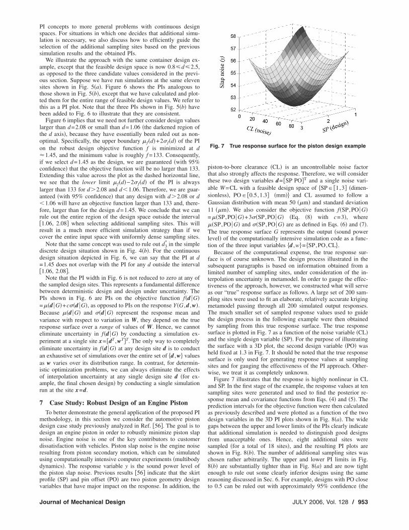
piston-to-bore clearance �CL� is an uncontrollable noise factorthat also strongly affects the response. Therefore, we will considerthese two design variables d= �SP PO�T and a single noise vari-able W=CL with a feasible design space of �SP� �1,3� �dimen-sionless�, PO� �0.5,1.3� �mm� and CL assumed to follow aGaussian distribution with mean 50 ��m� and standard deviation11 ��m�. We also consider the objective function f�SP,PO �G�=��SP,PO �G�+3��SP,PO �G� �Eq. �8� with c=3�, where��SP,PO �G� and ��SP,PO �G� are as defined in Eqs. �6� and �7�.The true response surface G represents the output �sound powerlevel� of the computationally intensive simulation code as a func-tion of the three input variables �d ,w= �SP,PO,CL.
Because of the computational expense, the true response sur-face is of course unknown. The design process illustrated in thesubsequent paragraphs is based on information obtained from alimited number of sampling sites, under consideration of the in-terpolation uncertainty in metamodel. In order to gauge the effec-tiveness of the approach, however, we constructed what will serveas our “true” response surface as follows. A large set of 200 sam-pling sites were used to fit an elaborate, relatively accurate krigingmetamodel passing through all 200 simulated output responses.The much smaller set of sampled response values used to guidethe design process in the following example were then obtainedby sampling from this true response surface. The true responsesurface is plotted in Fig. 7 as a function of the noise variable �CL�and the single design variable �SP�. For the purpose of illustratingthe surface with a 3D plot, the second design variable �PO� washeld fixed at 1.3 in Fig. 7. It should be noted that the true responsesurface is only used for generating response values at samplingsites and for gauging the effectiveness of the PI approach. Other-wise, we treat it as completely unknown.
Figure 7 illustrates that the response is highly nonlinear in CLand SP. In the first stage of the example, the response values at tensampling sites were generated and used to find the posterior re-sponse mean and covariance functions from Eqs. �4� and �5�. Theprediction intervals for the objective function were then calculatedas previously described and were plotted as a function of the twodesign variables in the 3D PI plots shown in Fig. 8�a�. The widegaps between the upper and lower limits of the PIs clearly indicatethat additional simulation is needed to distinguish good designsfrom unacceptable ones. Hence, eight additional sites weresampled �for a total of 18 sites�, and the resulting PI plots areshown in Fig. 8�b�. The number of additional sampling sites waschosen rather arbitrarily. The upper and lower PI limits in Fig.8�b� are substantially tighter than in Fig. 8�a� and are now tightenough to rule out some clearly inferior designs using the samereasoning discussed in Sec. 6. For example, designs with PO close
Fig. 7 True response surface for the piston design example
to 0.5 can be ruled out with approximately 95% confidence �the
JULY 2006, Vol. 128 / 953

lower limits of their PIs fall above the PI upper limits for manyother designs�. Hence, all further simulation can focus on themore promising designs. Note that as more and more samplingsites are added, the upper and lower PI limits will become tighterand tighter �Fig. 9 shows a one-dimensional counterpart after 27sampling sites�.
This can be more clearly visualized if we consider the designvariable PO to be discrete and construct three separate 2D plotsfor the three discrete values PO= �0.5,0.9,1.3, as shown in Fig.10. Note that the PI plots in Fig. 10 are precisely those in Fig. 8�b�for the three discrete values of PO. From Fig. 10 we can see thata portion of design region with PO=1.3, as well as the entiredesign region with PO=0.9 or 0.5, can be ruled out as inferior. Ifwe are only considering these three values for PO, the potentiallyoptimal design region then reduces to the much simpler 1D seg-ment shown in Fig. 10�a�. The dashed curves in Fig. 10 represent
Fig. 8 PI plots of robust design objective after: „a… 10 initialsimulation runs and „b… 18 simulation runs
Fig. 10 Three 2D cross sections of the PI plot in Fig.
ruled out „with 95% confidence… as inferior to the unsha954 / Vol. 128, JULY 2006
the true unknown objective function f�SP,PO �G=Gtrue�, withGtrue being that plotted in Fig. 7. Note that the PIs shown in Fig.10 all contain f�SP,PO �G=Gtrue�, although the true objectivefunction is sometimes closer to the boundary of the PI than to thecenter. This is all that we can expect, of course, given the defini-tion of a prediction interval.
Ruling out the inferior design regions �the shaded regions inFig. 10� and conducting nine additional simulations in the still-potentially optimal design region �1.5�SP�2.9, PO=1.3, wearrive at the PI plot shown in Fig. 9. Figure 9 indicates that we cannow narrow the optimal design down to a small neighborhoodaround d*= �PO*,SP*�= �1.3,2.333�. More specifically, if we ter-minate simulation at this point and choose d* as the optimal de-sign, we are guaranteed �with 95% confidence� that the true ob-jective function f�SP*,PO* �Gtrue� at the chosen design will fallwithin its PI range �54.24, 54.29�. If we decide that this range isnegligibly small, we would adopt d*= �1.3,2.333� as the final de-sign. For comparison, the optimal design based on the true re-sponse surface Gtrue is �PO=1.3, SP=2.334�.
8 Discussion
8.1 Selecting � and �. The prior distribution parameters �and � play an important role in quantifying the posterior uncer-tainty in the response surface G and therefore the uncertainty in
Fig. 9 PI plot after 27 simulation runs. The robust design so-lution †PO*=1.3, SP*=2.33‡ has an objective value within the PIof †54.24, 54.29‡.
…. All dark shaded regions of the design space can be
8„b ded design region shown in panel „a….Transactions of the ASME
the objective function f�d �G�. In particular, � and � influence thewidth of the PI. Because prior knowledge of appropriate valuesfor these parameters would generally be limited, we recommendestimating them directly from the sampling data. One methodwould be to use a full Bayesian approach in which we assumehyperprior distributions for the prior parameters �, �, and � andattempt to calculate the full posterior distribution G�d ,w� margin-alized over the posterior distribution of �, �, and �. Although thiswould provide the most accurate representation of interpolationuncertainty, the full posterior distribution of G would be far toocomplex to calculate analytically for even the simplest choice ofhyperpriors. The only recourse would be to use Monte Carlomethods to evaluate the posterior distribution of G. Using MonteCarlo simulation, Martin and Simpson �57� and Martin �58� dem-onstrated that for some typical situations the posterior distributionof G appears close to a t distribution and that Eq. �5� underesti-mates the posterior variance of G.
Although Monte Carlo methods are often feasible, for reasonsdiscussed in Sec. 8.2 they are far too computationally intensive tobe used for the problem addressed in this paper. In light of this,we recommend the same approximation that has been used in thevast majority of prior work on Bayesian analysis of computerexperiments �e.g, Refs. �27,28,43��. The approximation, which issometimes referred to as an empirical Bayes approach �59�, is tofirst calculate suitable estimates of the prior parameters �, �, and� and then simply treat the estimates as the true values in allsubsequent Bayesian computations. One might use maximumlikelihood estimates �MLEs� or assume hyperpriors for �, �, and� and then use their posterior means or modes as the estimates.Martin and Simpson �57� recommended using the posterior meansrather than the MLEs or posterior modes, because � and � oftenhave skewed distributions. The MLEs are simpler because theycan be readily obtained by maximizing the log-likelihood func-tion, which is equivalent to minimizing the function �yN
−H��T�−1�yN−H��−log�det����, where the ith-row, jth-columnelement of the N�N matrix � is �2R��si ,s j�, and all other quan-
tities are as defined in Sec. 3. Because the posterior mean � de-fined in Sec. 3 cannot be calculated until we have values for �and � available, some other suitable estimate for � should besubstituted into the log-likelihood function. For example, one mayuse the MLE of �, which is equivalent to jointly maximizing thelog likelihood over �, �, and �.
8.2 Monte Carlo Simulation Versus AnalyticalExpressions. As discussed in Sec 8.1, in order to obtain estimatesof the prior parameters �, �, and �, one approach is to calculatethe posterior distribution of �, �, and � and then use the posteriormean or mode as estimates. Although for certain assumed priordistributions, an analytical expression for the posterior distributionmight be tractable, one would often be forced to use Monte Carlosimulation to estimate the posterior distribution. Markov ChainMonte Carlo �MCMC� methods are particularly useful in this re-gard �59�. Martin and Simpson �57� used the Metropolis-HastingsMCMC method for such purposes.
For estimating the prior parameters, the computational burdenof Monte Carlo methods is quite reasonable. In contrast, for esti-mating the prediction intervals for constructing PI plots such asthose shown in Fig. 8, Monte Carlo methods �either Markov chainor conventional� would involve prohibitively large computationalexpense. In order to illustrate the reason, consider how one mightattempt to use Monte Carlo simulation to estimate the posteriormean � f�d� and standard deviation � f�d� for use in the PI of Eq.�15�: Consider the most optimistic scenario in which one alreadyhas available an expression for the posterior distribution of G,given the response values at a set of sampling sites. One wouldfirst discretize the entire �perhaps high dimensional� input �d ,wvariable space. For each replicate of the Monte Carlo simulation,
one would implement the following two steps: Step �1� GenerateJournal of Mechanical Design
one realization of the discretized random surface G over the entirespace of discretized input values �similar to those shown in Figs.2�a�–2�c�. Step �2� For each value of d in the discretized designvariable space, numerically integrate �using Eqs. �6� and �7�� andthe realization of G from step �1� over the entire discretized noisevariable space to obtain one realization of ��d �G�, ��d �G�, andf�d �G�. Steps �1� and �2� would then be repeated for some largenumber of Monte Carlo replicates �e.g., 10,000 or 100,000�, eachone corresponding to a different realization of G, to obtain theposterior distribution of f�d �G� empirically. From this, we couldestimate � f�d� and � f�d� and calculate a PI on f�d �G� for eachvalue of d.
To better appreciate the computational challenges, consider step�1�, and suppose we had ten input variables with the range foreach one discretized into 20 points �a relatively course discretiza-tion�. Because the entire input space is discretized into 2010
points, in order to generate one realization of G in step �1�, wewould have to generate 2010 random variables. Moreover, becausethe 2010 random variables are not independent of each other, wewould first have to calculate their 2010�1 mean vector and 2010
�2010 covariance matrix using Eqs. �4� and �5� Clearly, this iscomputationally prohibitive, especially when one considers that itmust be repeated for a large number of Monte Carlo replicates.Note that this is how the realizations of G shown in Fig 2 weregenerated, albeit for a much lower-dimensional problem.
One might consider replacing the numerical integration in step�2� with an “inner” Monte Carlo simulation loop in which wegenerate a large number of observations of W and empiricallyestimate ��d �G� and ��d �G� for each specific realization of Gfrom step �1�. Oakley and O’Hagan �54� discuss such an ap-proach, as well as some strategies for improving the computa-tional efficiency. For high-dimensional w, this would typically bemore computationally efficient than the numerical integration.However, the result would be a nested Monte Carlo simulation inwhich the inner simulation must be repeated for each value of d inthe design variable space, as well as for each replicate of the outersimulation loop �one replicate corresponding to one realization ofG�. Even with the computational improvements suggested in Ref.�54�, the nested Monte Carlo simulation is still far too computa-tionally expensive for high-dimensional design spaces.
If the numerical integration is replaced by a Monte Carlo simu-lation in the nested simulation scenario described above, onemight also consider combining the inner and outer simulations.This, however, is not possible given the nature of our predictioninterval formulation. By design, the prediction interval distin-guishes the effects of noise variable uncertainty �inner simulation�and interpolation uncertainty �outer simulation�.
For these reasons, Monte Carlo methods to estimate the predic-tion intervals are impractical, and analytical expressions becomemore important. An additional advantage of analytical expressionsis that they are better suited for design optimization algorithms.For example, we can differentiate the expressions to facilitate agradient search procedure. Monte Carlo sampling methods toevaluate design objective functions often result in jitter and slow�or non� convergence.
9 ConclusionsOn two parallel fronts, robust design under uncertainty and de-
sign optimization using computer experiments have both receiveda great deal of attention recently. When the two are combined,however, the “optimal” robust design solution may not be as ro-bust as it ought to be, because of the effects of metamodel inter-polation uncertainty. Moreover, the interpolation uncertainty can-not be eliminated with a final validation run, as it can indeterministic optimization problems. We have proposed a Baye-sian methodology with GRPs to represent the response surface inorder to clearly reveal the impact of interpolation uncertainty and
to directly quantify its effect on the robust design objective func-JULY 2006, Vol. 128 / 955

tion. This is particularly important for robust design using meta-models fitted to the output of computer experiments, because theconventional approach of estimating prediction uncertainty due tothe random error present in physical experiments is completelyinvalid with computer experiments. The Bayesian prediction in-tervals that we have derived can be used by designers as a simpleintuitive tool to quantify the effects of interpolation uncertainty,evaluate and compare robust design candidates, and guide a moreefficient simulation. One unique contribution is that our closed-form expressions for the prediction intervals obviate the need fornumerical integration and/or Monte Carlo simulation, which wehave argued is computationally infeasible in all but the simplestdesign problems, due to the curse of dimensionality.
Because we have only considered interpolation uncertainty, onemight view our treatment of model uncertainty as being relative toa base line that assumes the computer simulation is a perfect rep-resentation of reality. The approach is intended to ensure that thechosen design is close to what one would choose as optimal in thehypothetical scenario in which one were able to run an infinitenumber of simulations. Without an accurate assessment of theerror between reality and the output of the simulation code, it isobviously impossible to ensure that the chosen design will be evenclose to optimal when implemented in the physical world. Aproper treatment of this would involve a great many factors spe-cific to the application and the code and would naturally requiresome form of physical experimentation. If such were available,however, we believe that the Bayesian methodology that we haveutilized can be conveniently extended to encompass these otherforms of uncertainty. Bayesian statistical methods are often wellsuited for analyzing data obtained via physical experiments. It istypically straightforward to integrate uncertainty from multiplelevels in a hierarchical Bayesian analysis, with the posteriors fromone level becoming the priors at the next level. For guidelines ondefining and quantitatively representing various forms of uncer-tainty in computer experimentation and on their integrated analy-sis within a Bayesian framework, we refer the reader to the com-prehensive discussion in Kennedy and O’Hagan �43�.
It should be noted that although a low-dimensional design ex-ample was used to illustrate the approach throughout the paper,the closed-form expressions for the PIs and the concept of usingPIs to guide computer simulations and to distinguish the best de-sign alternative are applicable to high-dimensional problems. Theprimary challenge would lie in projecting the high-dimensional PIinformation down to meaningful three-dimensional PI plots. Pre-cisely how to do this is the subject of ongoing work.
Furthermore, we have only treated unconstrained optimization,for which we only need to consider uncertainty in the objectiveresponse. Typical design problems also have �i� constraint re-sponses that are functions of the inputs and that must be satisfiedwith a specified probability �when they are functionally dependenton uncertain noise variables�; and �ii� design variables that arethemselves uncertain, due perhaps to manufacturing variation. Webelieve that our approach can be readily extended to both of thesescenarios. Uncertain design variables can be treated simply bydecomposing each uncertain design variables into two compo-nents: A design component that represents the desired value forthe design variable, and a random noise component that representsthe difference between the actual design variable and its specifieddesired value. Regarding responses that must satisfy a constraintwith some specified probability: Constraint responses that are nor-mally viewed as random because they depend on the random Wcan simply be viewed as random because of their dependence onboth W and G. When selecting a design that ensures the constraintresponse is satisfied with a specified probability, we would con-sider the distribution of W and the posterior distribution of Ggiven the samples.
Throughout the paper, the implication has been that one can usethe prediction intervals to help ensure that the effect of interpola-
tion uncertainty is minimized, to the extent that it does not alter956 / Vol. 128, JULY 2006
the choice of optimal design. This would often involve runningadditional simulations in stages, guidelines and examples forwhich were presented in Secs. 5–7. If the effects of interpolationuncertainty are not negligible, but no additional simulation is pos-sible because of limited resources, then one would hope the finaldesign is robust to interpolation uncertainty, much like it is robustto noise uncertainty. One simple strategy for achieving this is touse the upper boundary of the prediction interval on f�d �G� �e.g.,the upper curve in Fig. 6� as the objective function in optimiza-tion. The upper boundary of the prediction interval representswhat we might view as the worst-case value �at the specifiedconfidence level for the prediction interval� of ��d �G�+c��d �G�,under direct consideration of interpolation uncertainty. As futureresearch, we are also exploring methods of considering interpola-tion uncertainty on par with noise uncertainty for decision makingin robust design.
AcknowledgmentThis work was supported in part by NSF Grants No. DMI
0354824 and No. DMI 0522662.
Nomenclatured � vector of design variables
W � vector of random noise variablesw � a specific value or realization of W
x= �d ,w � vector of design and noise variables togethery�x� � response surface as a function of xY�x� � response surface viewed as random
N � number of simulation runs conductedSN � set of N sampled sitesyN � vector of N simulated response values corre-
sponding to SN
y�x� � best Bayesian prediction of Y�x�pw�w� � pdf of W evaluated at wG�x� � Gaussian random process �GRP� to represent
uncertainty in the response surfacehT�x�� � prior mean function of G�x�
�2R��x ,x� � prior covariance function of G�x���d �G� � mean of Y�d ,W� with respect to W, given a
specific realization of G�2�d �G� � variance of Y�d ,W� with respect to W, given a
specific realization of Gf�d �G� � robust design objective function �e.g., ��d �G�
+c��d �G�����d� � mean of ��d �G� with respect to the random
process G���d� � standard deviation of ��d �G� with respect to
the random process G���d� � mean of ��d �G� with respect to the random
process G���d� � standard deviation of ��d �G� with respect to
the random process G� f�d� � mean of f�d �G� with respect to the random
process G� f�d� � standard deviation of f�d �G� with respect to
the random process GPI � prediction interval
Appendix: Derivation of the PI for the Robust DesignObjective Function
As discussed in Sec. 4, to obtain the PI for the objective func-tion f�d �G�=��d �G�+c��d �G�, we must calculate ���d�, ��
2 �d�,���d�, ��
2�d�, and Cov���d �G� ,��d �G��. The mean and variance
of ��d �G� are given by Eqs. �9� and �10�. For Gaussian noise, aTransactions of the ASME

polynomial h�x�, and the form of r�x� given by Eq. �3�, the termsy�d ,w�, Cov�Y�G ,d ,w� ,Y�G ,d ,w�� �yN� and pw�w� can all bewritten in terms of exponentials of quadratic forms of w, multi-plied by polynomials in w. Consequently, Eqs. �9� and �10� can beanalytically integrated to obtain closed-form expressions, insteadof evaluating them using numerical integration or Monte Carlosimulation. For example, suppose we have a single sampling siteand h�x�=1 and r�x�=exp�−�d�d−d1�2−�w�w−w1�2� In this
case, y�d ,w�= �+exp�−�d�d−d1�2−�W�w−w1�2�R−1�y1− ��,where only rT�x� is a function of w, while �, R−1 and yN areconstant with respect to w. y1 is the simulation output at samplingsite �d1 ,w1� and ��d ,�w� are the prior parameters. Thus from Eq.
�9�, one can obtain the analytical expression ���d�= �
+exp�−�d�d−d1�2� exp�−�ww12 / �2�w+1��R−1�y1− � / ��2�w+1.
The analytical expressions for general polynomial h�x� and r�x�of Eq. �3� can be obtained in a similar, albeit more tedious, man-ner.
To simplify notation, define S��2�d �G� and K�w ,w���Cov�Y�G ,d ,w� ,Y�G ,d� ,w�� �yN�, and omit the term “�yN” inthe following derivation, although it should be understood that theposterior distributions are all conditioned on the simulation outputyN. The mean of S is
�S�d� = EG��2�d�G�� = EG�Ew�G��Y�G,d,w� − ��d�G��2�G� .
After expanding the squared term, interchanging the order of theexpectation operators, and some tedious algebra, we obtain
�S = Ew�y�d,w� − ���d��2 +� K�w,w�pw�w�dw
−�� K�w,w��pw�w�dwpw�w��dw� �A1�
We can similarly obtain the variance of S as
Var�S� = 2�� �K�w,w���2pw�w�dwpw�w��dw�
− 4��� K�w,w��K�w,w��pw�w�dwpw�w��dw�
�pw�w��dw� +���� �K�w,w��K�w�,w��
+ K�w,w��K�w�,w���pw�w�dwpw�w��dw�
�pw�w��dw�pw�w��dw� + 4�� �y�d,w�
− ���d���y�d,w�� − ���d���K�w,w��
− 2� K�w�,w��pw�w��dw� +�� K�w�,w��pw�w��
�dwpw�w��dw��pw�w�dwpw�w��dw� �A2�
Because S����d �G��2, if we approximate ��d �G� as Gaussian�which is a better approximation than assuming �2�d �G� is nor-mal� we can express ���d� and ��
2�d� in terms of �S and Var�S�via
���d� = ��S2 − Var�S�/2�1/4, �A3�
and
��2�d� = �S − ��S
2 − Var�S�/2�1/2. �A4�
The covariance between ��d �G� and S��2�d �G� can be calcu-
lated from the identityJournal of Mechanical Design
Cov���d�G�,S� = EG���d�G�S� − ����d��S� .
By substituting in the definition of S, expanding the squaredterms, and interchanging the order of expectations, we obtain
Cov���d�G�,S� = ���d��Ew�y�d,w��2 + Ew�K�w,w�� − ����d��2
− 3EwEw��K�w,w��� + 2EwEw��y�d,w�K�w,w���
− ���d��S �A5�
From Eq. �A5�, if we further approximate ��d �G� and ��d �G�as jointly Gaussian, then from the relation betweenCov���d �G� ,��d �G�� and Cov���d �G� ,S�, we obtain
Cov���d�G�,��d�G�� = Cov���d�G�,S�/�2���d�� �A6�
For the same reasons stated above, Eqs. �A1�–�A6� can all beevaluated analytically. Hence, � f�d� and � f
2�d� can be calculatedfrom Eqs. �13� and �14�, and the prediction interval of f�d �G� isgiven by Eq. �15�.
References�1� Chang, K. H., Choi, K. K., Wang, J., Tsai, C. S., and Hardee, E., 1998, “A
Multilevel Product Model for Simulation-based Design of Mechanical Sys-tems,” Concurr. Eng. Res. Appl., 6�2�, pp. 131–144.
�2� Parry, J., Bornoff, R. B., Stehouwer, P., Driessen, L. T., and Stinstra, E., 2004,“Simulation-Based Design Optimization Methodologies Applied to CFD,”IEEE Trans. Compon., Hybrids, Manuf. Technol., 27�2�, pp. 391–397.
�3� Horstemeyer, M. F., and Wang, P., 2003, “Cradle-to-Grave Simulation-BasedDesign Incorporating Multiscale Microstructure-Property Modeling: Reinvigo-rating Design With Science,” J. Comput.-Aided Mater. Des., 10�1�, pp. 13–34.
�4� Parkinson, A., 1995, “Robust Mechanical Design Using Engineering Models,”ASME J. Mech. Des., 117�Sp. Iss. B�, pp. 48–54.
�5� Chen, W., Allen, J. K., Tsui, K. L., and Mistree, F., 1996, “A Procedure forRobust Design: Minimizing Variations Caused by Noise Factors and ControlFactors,” ASME J. Mech. Des., 118�4�, pp. 478–485.
�6� Du, X. P., and Chen, W., 2000, “Towards a Better Understanding of ModelingFeasibility Robustness in Engineering Design,” ASME J. Mech. Des., 122�4�,pp. 385–394.
�7� Thornton, A. C., 2001, “Optimism vs. Pessimism: Design Decisions in theFace of Process Capability Uncertainty,” ASME J. Mech. Des., 123�3�, pp.313–321.
�8� Suri, R., and Otto, K., 2001, “Manufacturing System Robustness ThroughIntegrated Modeling,” ASME J. Mech. Des., 123�4�, pp. 630–636.
�9� Kalsi, M., Hacker, K., and Lewis, K., 2001, “A Comprehensive Robust DesignApproach for Decision Trade-Offs in Complex Systems Design,” ASME J.Mech. Des., 123�1�, pp. 1–10.
�10� Hernandez, G., Allen, J. K., Woodruff, G. W., Simpson, T. W., Bascaran, E.,Avila, L. F., and Salinas, F., 2001, “Robust Design of Families of ProductsWith Production Modeling and Evaluation,” ASME J. Mech. Des., 123�2�, pp.183–190.
�11� McAllister, C. D., and Simpson, T. W., 2003, “Multidisciplinary Robust De-sign Optimization of an Internal Combustion Engine,” ASME J. Mech. Des.,125�1�, pp. 124–130.
�12� Du, X. P., and Chen, W., 2004, “Sequential Optimization and Reliability As-sessment Method for Efficient Probabilistic Design,” ASME J. Mech. Des.,126�2�, pp. 225–233.
�13� Gunawan, S., and Azarm, S., 2004, “Non-Gradient Based Parameter Sensitiv-ity Estimation for Single Objective Robust Design Optimization,” ASME J.Mech. Des., 126�3�, pp. 395–402.
�14� Koch, P. N., Yang, R. J., and Gu, L., 2004, “Design for Six Sigma ThroughRobust Optimization,” Struct. Multidiscip. Optim., 26�3–4�, pp. 235–248.
�15� Al-Widyan, K., and Angeles, J., 2005, “A Model-Based Formulation of RobustDesign,” ASME J. Mech. Des., 127�3�, pp. 388–396.
�16� Chen, W., Wiecek, M. M., and Zhang, J., 1999, “Quality Utility—A Compro-mise Programming Approach to Robust Design,” ASME J. Mech. Des.,121�2�, pp. 179–187.
�17� Du, X. P., Sudjianto, A., and Chen, W., 2004, “An Integrated Framework forOptimization Under Uncertainty Using Inverse Reliability Strategy,” ASME J.Mech. Des., 126�4�, pp. 562–570.
�18� Tu, J., Choi, K. K., and Park, Y. H., 2001, “Design Potential Method forRobust System Parameter Design,” AIAA J., 39�4�, pp. 667–677.
�19� Zou, T., Mahadevan, S., Mourelatos, Z., and Meernik, P., 2002, “ReliabilityAnalysis of Automotive Body-Door Subsystem,” Materialwiss. Werkstofftech.,78�3�, pp. 315–324.
�20� Youn, B. D., Choi, K. K., and Park, Y. H., 2003, “Hybrid Analysis Method forReliability-Based Design Optimization,” ASME J. Mech. Des., 125�2�, pp.221–232.
�21� Yang, R. J., Akkerman, A., Anderson, D. F., Faruque, O. M., and Gu, L., 2000,“Robustness Optimization for Vehicular Crash Simulations,” Rep. Sci. Res.Inst., 2�6�, pp. 8–13.
�22� Kleijnen, J. P. C., 1987, Statistical Tools for Simulation Practitioners, Marcel
Dekker, New York.JULY 2006, Vol. 128 / 957

�23� Simpson, T. W., Peplinski, J., Koch, P. N., and Allen, J. K., 2001, “Metamod-els for Computer Based Engineering Design: Survey and Recommendations,”Eng. Comput., 17�2�, pp. 129–150.
�24� Barthelemy, J.-F. M., and Haftka, R. T., 1993, “Approximation Concepts forOptimum Structural Design—A Review,” Struct. Optim., 5, pp. 129–144.
�25� Sobieszczanski-Sobieski, J., and Haftka, R. T., 1997, “Multidisciplinary Aero-space Design Optimization: Survey of Recent Developments,” Struct. Optim.,14, pp. 1–23.
�26� Box, G. E. P., Hunter, W. G., and Hunter, J. S., 1978, Statistics for Experi-menters, Wiley, New York.
�27� Sacks, J., Welch, W. J., Mitchell, T. J., and Wynn, H. P., 1989, “Design andAnalysis of Computer Experiments,” Stat. Sci., 4�4�, pp. 409–435.
�28� Currin, C., Mitchell, T., Morris, M. D., and Ylvisaker, D., 1991, “BayesianPrediction of Deterministic Functions, With Applications to the Design andAnalysis of Computer Experiments,” J. Am. Stat. Assoc., 86�416�, pp. 953–963.
�29� Hardy, R. L., 1971, “Multiquadratic Equations of Topography and Other Ir-regular Surfaces,” J. Geophys. Res., 76, pp. 1905–1915.
�30� Dyn, N., Levin, D., and Rippa, S., 1986, “Numerical Procedures for SurfaceFitting of Scattered Data by Radial Basis Functions,” SIAM �Soc. Ind. Appl.Math.� J. Sci. Stat. Comput., 7�2�, pp. 639–659.
�31� Mullur, A. A., and Messac, A., 2005, “Extended Radial Basis Functions: MoreFlexible and Effective Metamodeling,” AIAA J., 43�6�, pp. 1306–1315.
�32� Meckesheimer, M., Barton, R. R., Simpson, T., Limayen, F., and Yannou, B.,2001, “Metamodeling of Combined Discrete/Continuous Responses,” AIAAJ., 39�10�, pp. 1950–1959.
�33� Meckesheimer, M., Booker, A. J., Barton, R. R., and Simpson, T. W., 2002,“Computationally Inexpensive Metamodel Assessment Strategies,” AIAA J.,40�10�, pp. 2053–2060.
�34� Martin, J. D., and Simpson, T. W., 2005, “Use of Kriging Models to Approxi-mate Deterministic Computer Models,” AIAA J., 43�4�, pp. 853–863.
�35� Sasena, M. J., Papalambros, P., and Goovaerts, P., 2002, “Exploration of Meta-modeling Sampling Criteria for Constrained Global Optimization,” Eng. Op-timiz., 34�3�, pp. 263–278.
�36� Wang, G. G., 2003, “Adaptive Response Surface Method using inherited LatinHypercube Design points,” ASME J. Mech. Des., 125�2�, pp. 210–220.
�37� Romero, V. J., Swiler, L. P., and Giunta, A. A., 2004, “Construction of Re-sponse Surfaces Based on Progressive-Lattice-Sampling Experimental DesignsWith Application to Uncertainty Propagation,” Struct. Safety, 26�2�, pp. 201–219.
�38� Perez, V. M., Renaud, J. E., and Watson, L. T., 2004, “An Interior-Point Se-quential Approximate Optimization Methodology,” Struct. Multidiscip. Op-tim., 27�5�, pp. 360–370.
�39� Farhang Mehr, A., and Azarm, S., 2005, “Bayesian Meta-Modeling of Engi-neering Design Simulations: A Sequential Approach With Adaptation to Ir-regularities in the Response Behavior,” Int. J. Numer. Methods Eng., 62�15�,pp. 2104–2126.
�40� Lin, Y., Mistree, F., Allen, J. K., Tsui, K.-L., and Chen, V., 2004, “SequentialMetamodeling in Engineering Design,” AIAA/ISSMO Multidisciplinary Analy-sis and Optimization Conference, Albany, NY. Paper No. AIAA-2004-4304.
958 / Vol. 128, JULY 2006
�41� Gu, L., Yang, R. J., Tho, C. H., Makowski, M., Faruque, O., and Li, Y., 2001,“Optimization and Robustness for Crashworthiness of Side Impact,” Int. J.Veh. Des., 26�4�, pp. 348–360.
�42� Chen, W., Jin, R., and Sudjianto, A., 2005, “Analytical Global SensitivityAnalysis and Uncertainty Propagation for Robust Design,” J. Quality Technol.,in press.
�43� Kennedy, M. C., and O’Hagan, A., 2001, “Bayesian Calibration of ComputerExperiments,” J. R. Stat. Soc. Ser. B. Methodol., 63, pp. 425–464.
�44� Handcock, M. S., and Stein, M. L., 1993, “A Bayesian Analysis of Kriging,”Technometrics, 35, pp. 403–410.
�45� Jones, D. R., Schonlau, M., and Welch, W. J., 1998, “Efficient Global Optimi-zation of Expensive Black-Box Functions,” J. Global Optim., 13, pp. 455–492.
�46� Pacheco, J. E., Amon, C. H., and Finger, S., 2003, “Bayesian Surrogates Ap-plied to Conceptual Stages of the Engineering Design Process,” ASME J.Mech. Des., 125�4�, pp. 664–672.
�47� Jin, R., Du, X., and Chen, W., 2003, “The Use of Metamodeling Techniquesfor Optimization Under Uncertainty,” Struct. Multidiscip. Optim., 25�2�, pp.99–116.
�48� Duffin, R. J., Peterson, E. L., and Zener, C., 1967, Geometric Programming,Wiley, New York, p. 5.
�49� Steinberg, D. M., and Bursztyn, D., 2004, “Data Analytic Tools for Under-standing Random Field Regression Models,” Technometrics, 46�4�, pp. 411–420.
�50� Matheron, G., 1963, “Principles of Geostatistics,” Econ. Geol., 58, pp. 1246–1266.
�51� O’Hagan, A., 1992, “Some Bayesian Numerical Analysis,” in Bayesian Statis-tics 4, J. M. Bernardo, J. O. Berger, A. P. Dawid, and A. F. M. Smith, eds.Oxford University Press, New York, pp. 345–363.
�52� Montgomery, D. C., Peck, E. A., and Vining, G. G., 2001, Introduction toLinear Regression Analysis, 3rd ed., Wiley, New York.
�53� Haylock, R. G., and O’Hagan, A., 1996, “On Inference for Outputs of Com-putationally Expensive Algorithms With Uncertainty on the Inputs,” in Baye-sian Statistics 5 J. M. Bernardo, J. O. Berger, A. P. Dawid and A. F. M. Smith,eds. Oxford University Press, New York, pp. 629–37.
�54� Oakley, J., and O’Hagan, A., 2002, “Bayesian Inference for the UncertaintyDistribution of Computer Model Outputs,” Biometrika, 89�4�, pp. 769–784.
�55� Van Trees, H. L., 1968, Detection, Estimation, and Modulation Theory, Part I,Wiley, New York, p. 177.
�56� Jin, R., Chen, W., and Sudjianto, A., 2004, “Analytical Metamodel-BasedGlobal Sensitivity Analysis and Uncertainty Propagation for Robust Design,”SAE Trans. Journal of Materials and Manufacturing, paper 2004-01–0429.
�57� Martin, J. D., and Simpson, T. W., 2004, “A Monte Carlo Simulation of theKriging Model,” 10th AIAA/ISSMO Multidisciplinary Analysis and Optimiza-tion Conference, Albany, NY.
�58� Martin, J. D., 2005, “A Methodology for Evaluating System-level Uncertaintyin the Conceptual Design of Complex Multidisciplinary Systems,” Ph.D. the-sis, The Pennsylvania State University.
�59� Carlin, B. P., and Louis, T. A., 2000, Bayes and Empirical Bayes Methods forData Analysis, 2nd ed., Chapman & Hall/CRC, New York.
Transactions of the ASME