understanding the impacts and limitations of the current ...cecilia2050.eu/system/files/cecilia2050...
TRANSCRIPT
Understanding the impacts and limitations of the current instrument mix in detail: industrial sector
Choosing Efficient Combinations of Policy Instruments for Low-carbon
development and Innovation to Achieve Europe's 2050 climate targets

Page i | Understanding the impacts and limitations of the current instrument mix in detail: industrial sector
AUTHOR(S)
Mr Frédéric BRANGER, SMASH-CIRED
Mr Philippe QUIRION, CNRS, SMASH-CIRED
With contributions by:
Mr Julien CHEVALLIER, Université Paris 8
Project coordination and editing provided by Ecologic Institute.
Manuscript completed in October 2013
This document is available on the Internet at: [optional]
Document title Understanding the impacts and limitations of the current instrument mix in
detail: industrial sector
Work Package
Document Type
Date 9 October 2013
Document Status
ACKNOWLEDGEMENT & DISCLAIMER
The research leading to these results has received funding from the European Union FP7 ENV.2012.6.1-4: Exploiting the full potential of economic instruments to achieve the EU’s key greenhouse gas emissions reductions targets for 2020 and 2050 under the grant agreement n° 308680.
Neither the European Commission nor any person acting on behalf of the Commission is responsible for the use
which might be made of the following information. The views expressed in this publication are the sole
responsibility of the author and do not necessarily reflect the views of the European Commission.
Reproduction and translation for non-commercial purposes are authorized, provided the source is
acknowledged and the publisher is given prior notice and sent a copy.
Understanding the impacts and limitations of the current instrument mix in detail: industrial sector | Page ii
Table of Contents
1 Executive summary 5
2 Introduction 5
3 Did the EU ETS reduce CO2 emissions in the cement sector? 6
3.1 Introduction 6
3.2 Cement production process and potential for abatement 7
3.3 Data sources 9
3.4 Evidence 11
4 Carbon leakage and competitiveness of cement and steel industries under
the EU ETS 14
4.1 Introduction 14
4.2 Literature review 15
4.3 Industry contexts 17
4.3.1 Cement 17
4.3.2 Steel 18
4.4 Methodology and data 18
4.4.1 A simple analytical model 18
4.4.2 Estimated equation 20
4.5 Econometric techniques 21
4.6 Data 22
4.7 Results 23
4.7.1 Descriptive statistics 23
4.7.2 Regression results 27
5 Conclusion 30
Page iii | Understanding the impacts and limitations of the current instrument mix in detail: industrial sector
References 33
List of Tables
Table 1. Clinker volume by kiln type in the EU 28 (%) 13
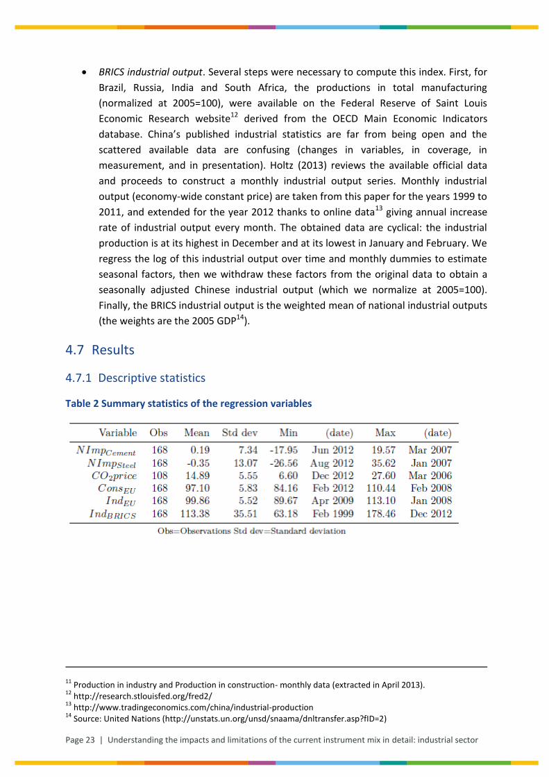
Table 2 Summary statistics of the regression variables 23
List of Figures
Figure 3-1 Potentials for CO2 abatement and leakage in the cement value chain 9
Figure 3-2 CO2 emissions in the cement and related sectors 10
Figure 3-3 Cement production and CO2 emissions in the EU 28 11
Figure 3-4 Drivers of cement specific emissions in the EU 28 12
Figure 4-1 EU allowance price 24
Figure 4-2 Cement net imports 25
Figure 4-3 Steel net imports 26
Figure 4-4 Other regression variables 26
Understanding the impacts and limitations of the current instrument mix in detail: industrial sector | Page iv
LIST OF ABBREVIATIONS
p.a. Per annum
GHG Greenhouse gas
WP Work Package
GNR Getting the Number Rights database
EUTL European Union Transaction Log
UNFCCC United Nations Framework Convention on Climate Change
IEA International energy Agency
WBCSD World Business council for Sustainable Development
Page 5 | Understanding the impacts and limitations of the current instrument mix in detail: industrial sector
1 Executive summary
We assess whether the EU ETS has reduced CO2 emissions in the cement sector, and whether
it has generated carbon leakage in the cement and steel sectors. A first conclusion, based on
the examination of the best available data, is that abatement from the EU ETS in the cement
sector, if any, has been very limited (maybe 2%). Analysing separately the drivers of
emissions, we conclude that:
o the EU ETS has not reduced the energy intensity of clinker production;
o there is no clear impact on the carbon intensity of the fuel mix;
o the EU ETS seems to have reduced the clinker ratio by approximately 2 percentage
points, compared to the historical trend.
A second conclusion is that the EU ETS has not generated carbon leakage, at least in the short
run (‘operational leakage’) in the cement and steel sectors. Our analysis on this point is based
on various econometric methods whose results converge, which provides confidence on the
results robustness.
2 Introduction
In the manufacturing industry, the main existing policy tool to reduce GHG emissions is the
EU ETS. Admittedly, at least in some member states, manufacturing industry is covered by
other policy instruments: carbon/energy taxes, regulatory measures or subsidies. Yet most
member States with carbon/energy taxes have exempted heavy industry and/or emission
sources covered by the ETS (as in Sweden and in Ireland, and as is currently planned in
France), while regulatory measures like those implemented in accordance to the IPPC
(Integrated Pollution Prevention and Control) directive mostly target other pollutants and
risks, rather than GHG. Finally, subsidies for GHG abatement in the manufacturing industry,
which are constrained by state aid rules, represent a much more limited implicit CO2 price
than the EU ETS.
Consequently, this deliverable focusses on the EU ETS, and in particular on the two main
manufacturing sectors covered by the scheme (measured by emissions, Kettner et al. 2013):
cement and steel. It contributes to the growing literature assessing the EU ETS ex post (cf.
Martin et al., 2012a, and references therein).
More specifically it addresses two questions: did the EU ETS reduce CO2 emissions in the
cement sector? Did it generate competitiveness losses and carbon leakage through
production offshoring in the cement and steel sectors? The first question (section 3) deals
Understanding the impacts and limitations of the current instrument mix in detail: industrial sector | Page 6
with the effectiveness of the ETS in these sectors while the second (section 4) is about
potential unintended consequences of the system. Section 5 concludes.
3 Did the EU ETS reduce CO2 emissions in the cement sector?
3.1 Introduction
Although a significant number of papers have assessed the effectiveness of the EU ETS, most
existing evaluations either remain at a very aggregate level or focus on the power sector:
there are very few estimates of the policy’s specific effect on manufacturing industry (Martin
et al., 2012a).
Ellerman and Feilhauer (2008) provide estimates of abatement due to the ETS in the German
manufacturing industry in phase I (about 6% of emissions in their calculation), but simply by
calculating the difference between the estimated aggregate abatement and the estimated
abatement in the power sector. Consequently, they acknowledge that this approach cannot
provide precise evidence.
A second study by Egenhofer et al. (2011) looks at the evolution of emission intensity (i.e.
emissions/gross value added) in the manufacturing sectors covered by the ETS in 2008 and
2009 and finds almost no evolution. More precisely the improvement in CO2 intensity was
lower in 2008 than in the preceding years (-0.4% vs. -2.3%) while it was higher in 2009 (-5.1%
vs. -2.3%), implying an abatement of less than 0.5% per annum over these two years, on
average. Notice that this study does not account for the changes in energy prices during the
period. Moreover it only considers the gross value added of manufacturing industry as a
whole while its sub-components, whose CO2 intensity widely differs, have had different
trends during the period considered.
Kettner et al. (2013) analyse two manufacturing industry sectors (cement and lime; pulp and
paper) up to 2010. Although emissions went down in both sectors, the main explanation is
the economic crisis which reduced demand and thus output. In addition, in pulp and paper,
the authors conclude that emissions have been reduced through a decrease in carbon
intensity, itself driven by fuel switch towards biomass and natural gas. In cement and lime,
they argue that the decrease in carbon intensity was driven by an increase in clinker imports
because, according to UNFCCC data, clinker emission intensity has been almost constant over
the period.
The other relevant study is Abrell et al. (2011) who estimate, at the firm level, reductions in
CO2 emissions around the transition from the first to the second phase. They assess EU ETS
firms’ emissions reduction in 2005-2006 compared to 2007-2008. The results indicate that
emission reductions between 2007 and 2008 were 3.6% larger than between 2005 and 2006.
According to the authors, the controls included in their estimation implied that this shift was
likely to be due to the change from Phase I to Phase II, and that it was not implied by a
proportionate decrease in production: emissions reductions were not caused only by
Page 7 | Understanding the impacts and limitations of the current instrument mix in detail: industrial sector
economic conditions or reductions in the economic activity of firms. However, the yearly
average spot CO2 price increased significantly from 2007 to 2008, while it decreased from
2005 to 2006, which also might explain the results. Taking a closer look at some sectors, the
authors conclude that basic metals and non-metallic minerals significantly increased their
reduction efforts between 2005-06 and 2007-08. More precisely, when controlling for
companies' turnover, number of employees, sector and home country, non-metallic minerals
firms increased their abatement by 8.7% and basic metals firms by 9.5%.
Hence, this review of the (limited) existing literature brings contradictory results. Abrell et al.
(2011) find a significant reduction in carbon intensity for basic metals (whose emissions occur
mostly in the steel sector) and non-metallic minerals (whose emissions occur mostly in the
cement sector) between 2007 and 2008 compared to 2005-2006. Yet Kettner et al. (2013)
find very limited reduction in carbon intensity in the cement and lime sector, and attribute
most of it to an increase in clinker imports – which implies carbon leakage. Moreover
Egenhofer et al. (2011) find almost no decrease in manufacturing industry’s carbon intensity
in 2008, which seems to contradict Abrell et al. (2011) results.
Explaining these contradictions is difficult since the studies use different datasets for
emissions (CITL or UNFCCC) and for economic activity. This calls for a careful analysis of the
emissions and production data. Moreover, longer time series, and in some cases more
accurate data sources, are available than those used in these studies, especially in the
cement sector. Hence, in the following, we present an original study based on longer time
series (up to 2011) and as we shall argue a more accurate database, but in the conclusion of
this third section we come back to the results of the above-mentioned studies.
3.2 Cement production process and potential for abatement
In the cement sector, CO2 emissions occur during the production of clinker, an intermediate
product which constitutes about 75% of cement in mass, and which is only used to produce
cement. Clinker is produced by heating limestone in a rotating kiln. In the oldest kilns, some
of which are still in operation, limestone is introduced as slurry (‘wet production route’) while
in more recent ones, it is introduced as a powder (‘dry production route’) which consumes
less energy since less water has to be evaporated. In addition, in recent kilns, part of the
waste heat is recovered (pre-heating and pre-calcining of raw material). Around 40% of CO2
emissions are due to the burning of fossil fuel. Any fuel can be used, so operators choose the
cheapest ones, mostly pulverised coal or petroleum coke (petcoke) in Europe, with also some
‘alternative fuels’, i.e. various types of waste or biomass. The remaining 60% are process
emissions, i.e. due to the chemical reaction itself: the transformation of limestone into
clinker generates around 0.53 t CO2/t clinker (a little more for clinker used in some special
products like white cement).
Clinker is then grinded and mixed with other materials, mostly limestone, gypsum, puzzolana,
blast furnace slag (a by-product of steelmaking), and fly ash from power plants. The share of
Understanding the impacts and limitations of the current instrument mix in detail: industrial sector | Page 8
these other components, the production of which does not emit much CO21, currently
reaches 25% in average in Europe and 32% in Brazil (WBCSD, 2013). Traditional Portland
cement is made of 95% of clinker while ‘blended’ cement includes a higher rate of other
components.
Alternative cements, produced without clinker, exist, and some of them have been available
for more than a century. However, their production is extremely limited compared to
Portland or blended cements. Whether their development is mostly hindered by inertia in
business practice and specifications for building materials, or by more fundamental reasons
like unproven durability or higher cost, remains an open question. Juenger et al. (2011)
provide an up-to-date synthesis of the advances in alternative cements.
Cement – whether Portland, blended or alternative – is then mixed with other mineral
elements to form concrete, a building material. This quick overview of the production process
allows identifying the various options available to reduce CO2 emissions from cement
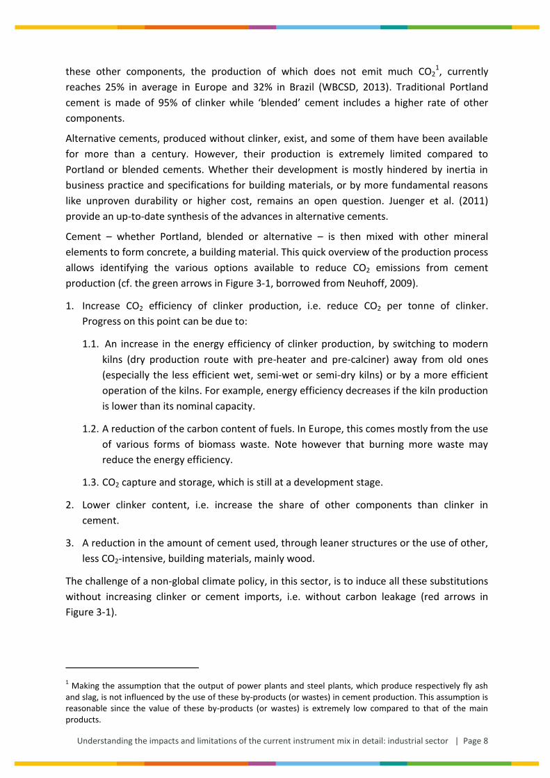
production (cf. the green arrows in Figure 3-1, borrowed from Neuhoff, 2009).
1. Increase CO2 efficiency of clinker production, i.e. reduce CO2 per tonne of clinker.
Progress on this point can be due to:
1.1. An increase in the energy efficiency of clinker production, by switching to modern
kilns (dry production route with pre-heater and pre-calciner) away from old ones
(especially the less efficient wet, semi-wet or semi-dry kilns) or by a more efficient
operation of the kilns. For example, energy efficiency decreases if the kiln production
is lower than its nominal capacity.
1.2. A reduction of the carbon content of fuels. In Europe, this comes mostly from the use
of various forms of biomass waste. Note however that burning more waste may
reduce the energy efficiency.
1.3. CO2 capture and storage, which is still at a development stage.
2. Lower clinker content, i.e. increase the share of other components than clinker in
cement.
3. A reduction in the amount of cement used, through leaner structures or the use of other,
less CO2-intensive, building materials, mainly wood.
The challenge of a non-global climate policy, in this sector, is to induce all these substitutions
without increasing clinker or cement imports, i.e. without carbon leakage (red arrows in
Figure 3-1).
1 Making the assumption that the output of power plants and steel plants, which produce respectively fly ash
and slag, is not influenced by the use of these by-products (or wastes) in cement production. This assumption is reasonable since the value of these by-products (or wastes) is extremely low compared to that of the main products.
Page 9 | Understanding the impacts and limitations of the current instrument mix in detail: industrial sector
Figure 3-1 Potentials for CO2 abatement and leakage in the cement value chain
Source: Neuhoff (2009)
The leakage issue will be dealt with in section 4. Before that, in this third section, we discuss
how these drivers of emissions have evolved in the EU before and after the start of the EU
ETS, in order to shed some light on the ETS efficiency.
3.3 Data sources
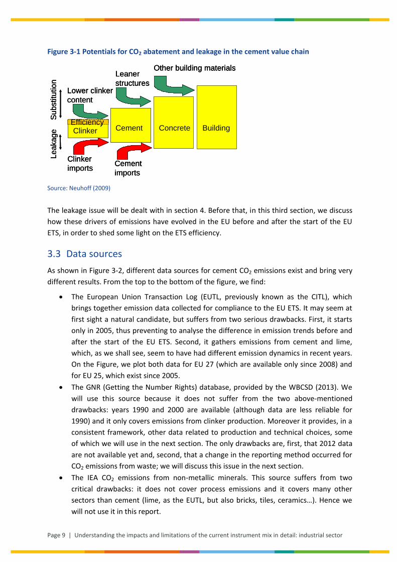
As shown in Figure 3-2, different data sources for cement CO2 emissions exist and bring very
different results. From the top to the bottom of the figure, we find:
The European Union Transaction Log (EUTL, previously known as the CITL), which
brings together emission data collected for compliance to the EU ETS. It may seem at
first sight a natural candidate, but suffers from two serious drawbacks. First, it starts
only in 2005, thus preventing to analyse the difference in emission trends before and
after the start of the EU ETS. Second, it gathers emissions from cement and lime,
which, as we shall see, seem to have had different emission dynamics in recent years.
On the Figure, we plot both data for EU 27 (which are available only since 2008) and
for EU 25, which exist since 2005.
The GNR (Getting the Number Rights) database, provided by the WBCSD (2013). We
will use this source because it does not suffer from the two above-mentioned
drawbacks: years 1990 and 2000 are available (although data are less reliable for
1990) and it only covers emissions from clinker production. Moreover it provides, in a
consistent framework, other data related to production and technical choices, some
of which we will use in the next section. The only drawbacks are, first, that 2012 data
are not available yet and, second, that a change in the reporting method occurred for
CO2 emissions from waste; we will discuss this issue in the next section.
The IEA CO2 emissions from non-metallic minerals. This source suffers from two
critical drawbacks: it does not cover process emissions and it covers many other
sectors than cement (lime, as the EUTL, but also bricks, tiles, ceramics…). Hence we
will not use it in this report.
Clinker Cement Concrete Building
Other building materialsLeaner
structuresLower clinker
content
Substitu
tion
Clinker
importsCement
imports
Leakage
EfficiencyClinker Cement Concrete Building
Other building materialsLeaner
structuresLower clinker
content
Substitu
tion
Other building materialsLeaner
structuresLower clinker
content
Substitu
tion
Clinker
importsCement
imports
Leakage
Clinker
importsCement
imports
Leakage
EfficiencyEfficiency
Understanding the impacts and limitations of the current instrument mix in detail: industrial sector | Page 10
The UNFCCC gathers national inventories for Annex I countries, among which EU
member states. These inventories identify process emissions from clinker production
(category 2.A.1), but not fossil fuel emissions, which are gathered with other sectors.
This explains why this curve is below the others and prevents from analysing energy
intensity and fuel switch as emission drivers.
For all these reasons, we choose to rely on the GNR database.
Figure 3-2 CO2 emissions in the cement and related sectors
70
90
110
130
150
170
190
Mt
CO
2
EUTL Cement/Lime (code 6) + Clinker (code 29) - EU 27
EUTL Cement/Lime (code 6) + Clinker (code 29) - EU 25
GNR gross CO2 emissions EU28
IEA CO2 emissions non-metallic minerals EU 27
UNFCCC Process emissions 2.A.1 EU 27
Page 11 | Understanding the impacts and limitations of the current instrument mix in detail: industrial sector
3.4 Evidence
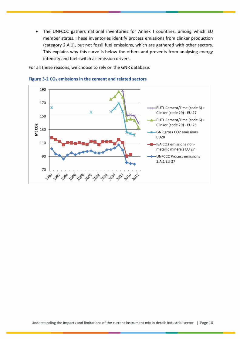
Figure 3-3 Cement production and CO2 emissions in the EU 28
Source: authors’ calculation based on WBCSD (2013) data.
Let’s start by looking at CO2 emissions. As shown in Figure 3-3, after being rather stable
between 1990 and 2007, they drop heavily from 2007 and 2009 (from 170 to 126 Mt) then
stabilise again. However, although this drop coincides with the second phase of the EU ETS, it
is mainly due the recession, which entailed a large decrease in cement production (from 260
Mt in 2007 to 186 in 2010). Taking the ratio of these two series yields cement specific
emission, expressed in t CO2/t cement produced. It has evolved in a much less glorious way:
whereas it decreased neatly from 1990 to 2000 (-5 kg CO2/t cement p.a. i.e. -0.7% p.a.) and
even more between 2000 to 2005 (-7 kg CO2/t cement p.a. i.e. -1% p.a.), it has stalled since
the start of the EU ETS: (-2 kg CO2/t cement p.a. i.e. -0.33% p.a. between 2005 and 2011).
Moreover, as we shall see, a change in CO2 emissions reporting requirements between 2010
and 2011 entails an artificial decrease in emissions between these years. If we limit ourselves
to the period 2005-2010, not concerned with this artefact, there has actually been an
increase in specific emissions. In any case, CO2 emissions per tonne of cement have been
almost steady since 2005.
Of course, on the sole basis of these data, one cannot exclude that the EU ETS reduced
emissions already in 2005, its first year of operation, but given the investments needed both
in cement plants (to increase energy efficiency, to process slag or fly ash or to allow burning
more biomass and waste), or to convince customers to switch to cements with a lower
clinker content, this seems unlikely unless one thinks that the reductions were triggered
earlier. We cannot completely exclude this possibility but proxy data like process emissions
0,58
0,6
0,62
0,64
0,66
0,68
0,7
0,72
0,74
0,76
0
50
100
150
200
250
3001
99
0
19
91
19
92
19
93
19
94
19
95
19
96
19
97
19
98
19
99
20
00
20
01
20
02
20
03
20
04
20
05
20
06
20
07
20
08
20
09
20
10
20
11
t C
O2
/t c
em
en
t
Mt/
yr.
Cement production
CO2 emissions
t CO2/t cement (right axis)
Understanding the impacts and limitations of the current instrument mix in detail: industrial sector | Page 12
from the UNFCCC and fossil fuel emissions in the non-metallic minerals sectors from the IEA
do not show any particular inflexion between 2004 and 2005.
How did the drivers that we have presented in section 3.2.1 contribute to the evolution of
cement CO2 intensity? Cement production (driver n° 3) did not, by definition (except
indirectly – see below), and neither did CO2 capture and storage since it is still at a pilot stage.
Figure 3-4 below displays the evolution of the remaining three drivers: energy intensity of
clinker production (driver n° 1.1), carbon intensity of the fuel mix (driver n° 1.2) and clinker
ratio (driver n°2).
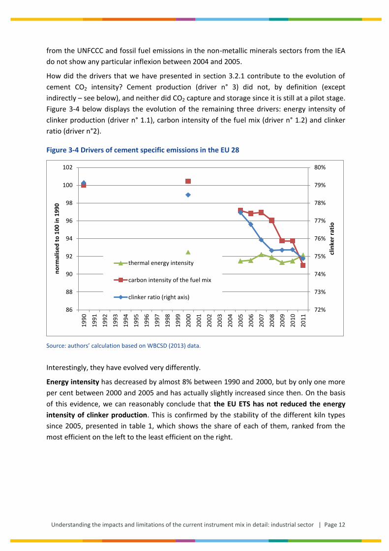
Figure 3-4 Drivers of cement specific emissions in the EU 28
Source: authors’ calculation based on WBCSD (2013) data.
Interestingly, they have evolved very differently.
Energy intensity has decreased by almost 8% between 1990 and 2000, but by only one more
per cent between 2000 and 2005 and has actually slightly increased since then. On the basis
of this evidence, we can reasonably conclude that the EU ETS has not reduced the energy
intensity of clinker production. This is confirmed by the stability of the different kiln types
since 2005, presented in table 1, which shows the share of each of them, ranked from the
most efficient on the left to the least efficient on the right.
72%
73%
74%
75%
76%
77%
78%
79%
80%
86
88
90
92
94
96
98
100
102
19
90
19
91
19
92
19
93
19
94
19
95
19
96
19
97
19
98
19
99
20
00
20
01
20
02
20
03
20
04
20
05
20
06
20
07
20
08
20
09
20
10
20
11
clin
ker
rati
o
no
rmal
ise
d t
o 1
00
in 1
99
0
thermal energy intensity
carbon intensity of the fuel mix
clinker ratio (right axis)
Page 13 | Understanding the impacts and limitations of the current instrument mix in detail: industrial sector
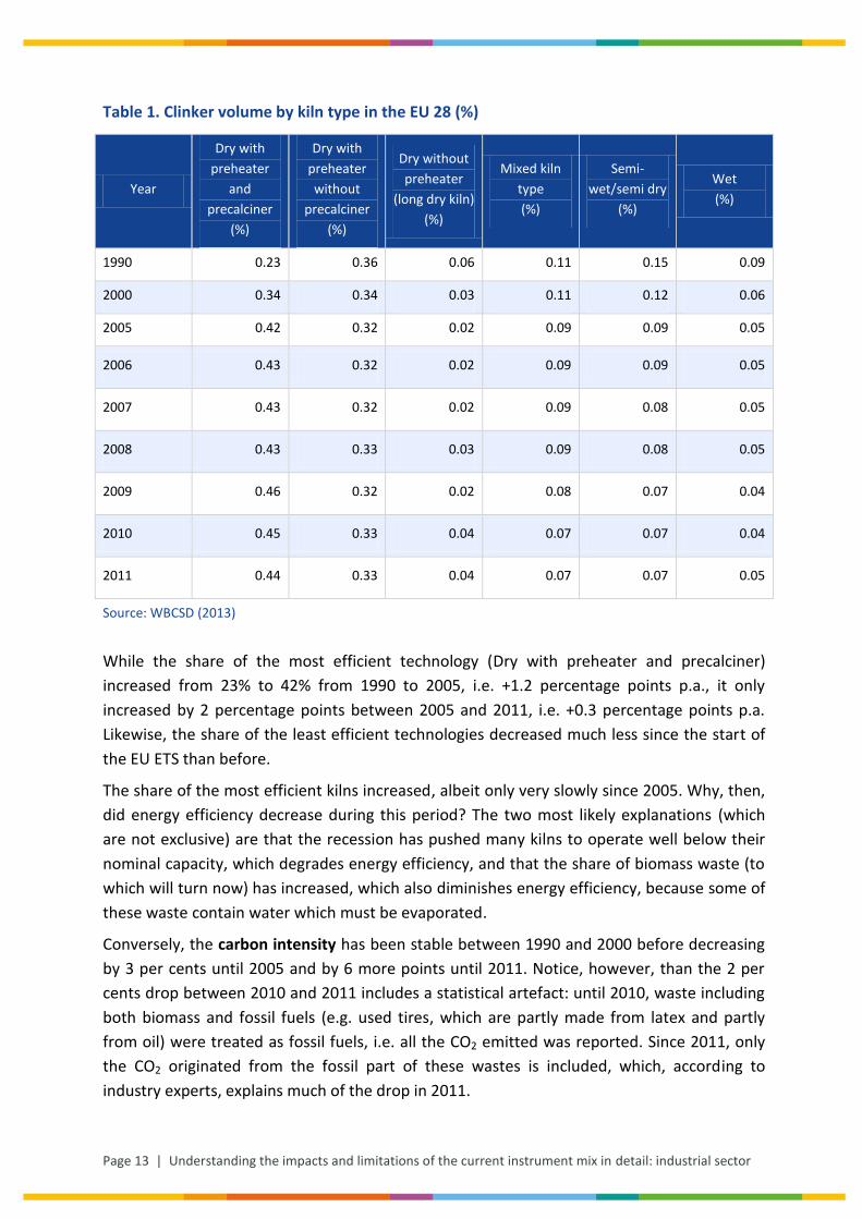
Table 1. Clinker volume by kiln type in the EU 28 (%)
Year
Dry with
preheater
and
precalciner
(%)
Dry with
preheater
without
precalciner
(%)
Dry without
preheater
(long dry kiln)
(%)
Mixed kiln
type
(%)
Semi-
wet/semi dry
(%)
Wet
(%)
1990 0.23 0.36 0.06 0.11 0.15 0.09
2000 0.34 0.34 0.03 0.11 0.12 0.06
2005 0.42 0.32 0.02 0.09 0.09 0.05
2006 0.43 0.32 0.02 0.09 0.09 0.05
2007 0.43 0.32 0.02 0.09 0.08 0.05
2008 0.43 0.33 0.03 0.09 0.08 0.05
2009 0.46 0.32 0.02 0.08 0.07 0.04
2010 0.45 0.33 0.04 0.07 0.07 0.04
2011 0.44 0.33 0.04 0.07 0.07 0.05
Source: WBCSD (2013)
While the share of the most efficient technology (Dry with preheater and precalciner)
increased from 23% to 42% from 1990 to 2005, i.e. +1.2 percentage points p.a., it only
increased by 2 percentage points between 2005 and 2011, i.e. +0.3 percentage points p.a.
Likewise, the share of the least efficient technologies decreased much less since the start of
the EU ETS than before.
The share of the most efficient kilns increased, albeit only very slowly since 2005. Why, then,
did energy efficiency decrease during this period? The two most likely explanations (which
are not exclusive) are that the recession has pushed many kilns to operate well below their
nominal capacity, which degrades energy efficiency, and that the share of biomass waste (to
which will turn now) has increased, which also diminishes energy efficiency, because some of
these waste contain water which must be evaporated.
Conversely, the carbon intensity has been stable between 1990 and 2000 before decreasing
by 3 per cents until 2005 and by 6 more points until 2011. Notice, however, than the 2 per
cents drop between 2010 and 2011 includes a statistical artefact: until 2010, waste including
both biomass and fossil fuels (e.g. used tires, which are partly made from latex and partly
from oil) were treated as fossil fuels, i.e. all the CO2 emitted was reported. Since 2011, only
the CO2 originated from the fossil part of these wastes is included, which, according to
industry experts, explains much of the drop in 2011.
Understanding the impacts and limitations of the current instrument mix in detail: industrial sector | Page 14
Without this artefact, the carbon intensity of clinker production has decreased at the same
rate between 2000 and 2005 and between 2005 and 2010 (0.7 percentage points p.a.).
Without the inclusion of the cement sector in the EU ETS, this decrease may have been
slower, in particular because other sectors (mainly electricity generation) may have burnt
some of the biomass fuel which was actually used by the cement sector. Still, there is no
clear impact of the EU ETS on carbon intensity. The explanation may be that the CO2 price
has been insufficient: as explained in a forthcoming Climate Strategies (2013) report, even
with a CO2 price of 20€ (higher than the observed average spot price), replacing a wet or
semi-wet kiln with a state-of-the-art kiln leads to cost savings of 4.6 and 1.4 €/t clinker
respectively, which may be insufficient for justifying retrofitting. Moreover, one cannot
exclude a perverse impact from the free allowance allocation, by which some companies
would refrain from reducing emissions, anticipating future allocation to be proportional to
future emissions.
Finally, the clinker ratio has decreased only slightly (by less than one percentage point)
between 1990 and 2000, and at a faster rate since then, especially between 2005 and 2008
(by 2.2 percentage points). After a phase of stability between 2008 and 2010, the ratio
decreased again in 2011, by 0.5 percentage points. In average, it decreased annually by 0.09
percentage points over 1990-2000, by 0.24 percentage points over 2000-2005 and by 0.55
percentage points over 2005-2011. Hence, the EU ETS seems to have significantly reduced
the clinker ratio. If the ratio had followed its 2000-2005 trend, it would have been around 2
percentage points higher than its actual value in 2011, resulting in emissions approximately
2% higher. However, we cannot rule out another explanation, i.e. the massive increase in
steam coal and petcoke price (the two main energy carriers used to produce clinker) since
2000. Both prices have roughly doubled from 2003-4 to 2010-11 (Cembureau, 2011, p. 31),
reinforcing the profitability of using substitutes rather than clinker.
4 Carbon leakage and competitiveness of cement and steel
industries under the EU ETS
4.1 Introduction
Unfortunately, the existing evidence about the amount of carbon leakage and
competitiveness losses which can be expected from a given climate policy is not conclusive
(cf. section 4.2 below): among ex ante studies, general equilibrium models point to a positive
but limited leakage at the aggregate level (typically from 5% to 25%) while for some carbon-
intensive sectors like steel or cement, a higher leakage rate is sometimes forecast
(Oikonomou et al., 2006; Demailly and Quirion, 2006), although this is not always true:
Demailly and Quirion (2008) find a 0.5%-25% uncertainty range for steel. Moreover, the few
existing ex post studies do not bring consistent conclusions. Finally, ex ante as well as ex post
Page 15 | Understanding the impacts and limitations of the current instrument mix in detail: industrial sector
studies assess different policy scenarios in different contexts so cannot be directly used to
assess the impact of the EU ETS.
The present section aims at filling this gap by assessing econometrically operational leakage2
over the first two phases of the EU ETS, in the two most emitting manufacturing industry
sectors: cement and steel. The methodology is to econometrically estimate a relation,
obtained via an analytic model, between net imports (imports minus exports) and the carbon
price, controlling for other factors that may influence net imports such as economic activity
in and outside Europe. Using two different econometric techniques which provide consistent
results, we conclude that net imports of cement and steel have been driven by domestic and
foreign demand but not by the CO2 allowance price, falsifying the claim that the ETS has
generated leakage, at least in the short run.
4.2 Literature review
Whereas carbon pricing is relatively new, environmental regulations on local pollutants have
a much longer history. For example the Clean Air Act was implemented in the US during the
seventies, well before climate change was on the agenda. Therefore the first studies
empirically assessing the impacts of environmental regulations on trade dealt with local
pollution issues and tested the pollution haven hypothesis/effect (Kalt, 1988; Tobey, 1990;
Grossman and Krueger, 1993; Jaffe et al., 1995). The migration of dirty industries to countries
with lower environmental standards (pollution havens) depends both on the environmental
regulatory gap and on trade tariffs. In the pollution haven hypothesis (respectively effect),
the first (respectively the second) factor is hold constant3. The pollution haven hypothesis
was a major concern during the negotiations of the North American Free Trade Agreements
in the nineties (Jaffe et al., 1995), but as the decrease in trade tariffs seems to slow down, the
pollution haven effect is nowadays a more relevant concern (and carbon leakage due the EU
ETS would be a ‘carbon haven effect’ (Branger and Quirion, 2013a)).
The prevailing conclusion of the pollution haven literature is that environmental regulations
have a small to negligible impact on relocations (Oikonomou et al., 2006). After a first wave
of inconclusive works (Eskeland and Harrison, 2003), a second generation of studies have
demonstrated statistically significant but small pollution haven effects using panels of data
and industry or country fixed effects (Levinson and Taylor, 2008). Many reasons were invoked
to explain why the widely believed fear of environmental relocations was not observed.
Some pointed that environmental regulations are not a main driver of relocations contrarily
to economic growth in emerging countries (Smarzynska, 2002), or that pollution abatement
represents a small fraction of costs compared to other costs or barriers which still favour
production in industrialized countries (Oikonomou et al., 2006): tariffs, transport costs,
labour productivity, volatility in exchange rate, political risk, etc. Other highlighted that heavy
2 A distinction can be made between leakage that occurs in the presence of capacity constraints in the short
term, termed operational leakage and leakage which occurs in the longer term via the impacts of the EU-ETS on investment policy, termed investment leakage (Climate Strategies, 2013). 3 For a more elaborated presentation and discussion of these notions, cf. Kuik et al. (2013).
Understanding the impacts and limitations of the current instrument mix in detail: industrial sector | Page 16
industries are very capital-intensive and tend to locate in capital-abundant countries, or that
their capital intensity made them less prone to relocate than ‘footloose’ industries
(Ederington et al., 2003). Finally, the Porter hypothesis (Porter and Van der Linde, 1995),
implying that regulations bring cost-reducing innovations, was also mentioned.
The pollution haven literature is mostly related to command-and-control regulations for local
pollutants, whereas the EU ETS is a cap-and-trade system for carbon emissions. Some studies
evaluated policies which are closer to the EU ETS such as environmental taxation in some
European countries. Miltner and Salmons (Miltner and Salmons, 2009) studied the impact of
environmental tax reforms (ETR) on competitiveness indicators for 7 European countries and
8 sectors and found that, out of 56 cases (7 countries and 8 sectors studied), the impact of
ETR on competitiveness was insignificant in 80% of the cases, positive in 4% and negative for
only 16% of the cases (Miltner and Salmons 2009). However, energy-intensive sectors
benefited from exemptions and lower taxation rates. Costantini and Mazzanti (2012) used a
gravity model to analyse the impact on trade flows of environmental and innovation policies
in Europe and revealed a Porter-like mechanism: when the regulatory framework is well
followed by private innovation, environmental policies seem to foster rather than undermine
export dynamics.
The question of carbon leakage was also a relevant issue for the Kyoto protocol. Aichele and
Felbermayr (2012) assessed the impact of the Kyoto protocol on CO2 emissions, CO2 footprint
and CO2 net imports, using a differences-in-differences approach. They conclude that the
Kyoto protocol has reduced domestic emissions by about 7% but has not changed the carbon
footprint: CO2 net imports increased by about 14%. Although they do not explicitly formulate
it, their results lead to a carbon leakage estimation of about 100%, contrasting with the other
empirical studies. However, two caveats are in order. First, China became a member of the
WTO in 2002, just when most developed countries ratified the protocol. Since most CO2 net
imports are due to trade with China, the rise in net imports may well be due to China WTO
membership rather than to Kyoto. Second, apart from those covered by the EU ETS, countries
with a Kyoto target have not adopted significant policies to reduce emissions in
manufacturing industry. Hence, if Kyoto had caused leakage (through the competitiveness
channel), it should show up on the CO2 net imports of countries covered by the EU ETS rather
than on CO2 net imports of countries covered by a Kyoto target; yet the authors report that
EU membership does not increase CO2 imports, when they include both EU membership and
the existence of a Kyoto target in the regression.
Some papers use econometric models to empirically investigate the impact of climate policies
on heavy industries ex ante, using energy prices as a proxy. Gerlagh and Mathys (2011)
studied the links between energy abundance and trade in 14 countries in Europe, Asia and
America. They found that energy is a major driver for sector location through specialisation,
but do not quantify relocations under uneven carbon policies. Aldy and Pizer (2011) focused
on the US but used a richer sectoral disaggregation. The authors conclude that a $15 CO2
price would not significantly impact the US manufacturing industry as a whole, but that some
sectors would be harder hit with a decrease of about 3% in their production.
Page 17 | Understanding the impacts and limitations of the current instrument mix in detail: industrial sector
The EU ETS has constituted a subject of research for a body of empirical studies on different
topics: abatement estimation (Ellerman and Buchner, 2008; Delarue et al., 2008), impact of
investment and innovation (Calel and Dechezleprêtre, 2012; Martin et al., 2012b),
distributional effects (Sijm et al. 2006, de Bruyn et al. 2010, Alexeeva-Talebi 2011),
determinants of the CO2 price (Alberola et al., 2008; Mansanet-Bataller et al., 2011;
Hintermann, 2010), and carbon leakage.
So far, the few existing empirical ex post studies have not revealed any statistical evidence of
carbon leakage and competitiveness losses for heavy industries in the EU ETS. Zachman et al.
(2011), using firm level panel data and a matching procedure between regulated and
unregulated firms, found no evidence that the ETS affected companies’ profits. Studying the
impact of carbon price on trade flows, several studies found no evidence of competitiveness-
driven operational leakage for the different sectors at risk of the EU ETS: aluminium (Reinaud,
2008a; Sartor, 2013; Ellerman et al., 2010; Quirion, 2011), oil refining (Lacombe, 2008),
cement and steel (Ellerman et al., 2010; Quirion, 2011).
Our work goes beyond the above-mentioned studies on several points. First, more data is
available as the EU ETS is entering its third phase after eight years of functioning. Second, we
introduce a new variable as a proxy for demand outside the EU, which improves the
explanatory power of the econometric model. Third, the estimated equations are based on a
structural economic model. Finally, we use several time-series regression techniques, to
assess the results robustness.
4.3 Industry contexts
Cement and steel share the common aspect to be heavy industries impacted by the EU ETS.
They are the two largest CO2 emitters among European manufacturing sectors, with
respectively 10% and 9% of the allowances allocations in the EU ETS (Kettner et al., 2013).
However they rank differently along the two dimensions generally retained to assess whether
a sector is at risk of carbon leakage, i.e. carbon intensity and openness to international trade
(Hourcade et al., 2007; Juergens et al., 2013): cement is very carbon-intensive but only
moderately open to international trade while steel features lower carbon intensity but higher
trade openness.
4.3.1 Cement
As we have seen in section 3.2, calcination of limestone and burning of fossil fuel (mainly coal
and petcoke) make the cement manufacturing process very carbon-intensive (around 650 kg
of CO2 per tonne). Cement production embodies 5% of worldwide emissions.
The raw material of cement, limestone, is present in abundant quantities all over the world.
Besides, the value-added per tonne of cement is relatively low. Because of these two
features, cement is produced in virtually all countries around the world and is only
moderately traded internationally (only 3.8% of cement was traded internationally in 2011
(ICR, 2012)). China represents the lion’s share of cement consumption and production around
the world, due to the large scale developments and infrastructure build-up projects that the
Understanding the impacts and limitations of the current instrument mix in detail: industrial sector | Page 18
Chinese government is undertaking. In 2011, 57% of the 3.6 billion tonnes of cement were
produced in China, and the second country producer, the EU, was far behind with 8% of the
world production (ICR, 2012).
Cement is a sector where international competition is low (Selim and Salem, 2010). Because
of low value per tonne and market concentration, important price differences remain even
within Europe (Ponssard and Walker, 2008). Prices are higher and producers have more
market power inland than near the coasts because transportation costs are much lower by
sea than by road.
Clinker is the major raw material for cement. Its production accounts for most of the CO2
emitted in the manufacturing process, and it can be transported more easily than cement
since its handling emits less dust. Therefore in the cement sector, carbon leakage is more
likely to happen through clinker trade than through cement trade.
4.3.2 Steel
Steel is produced either from iron ore and coal using the Blast Furnace - Basis Oxygen
Furnaces (BF-BOF) route, for around 70% of world production, or from steel scrap in Electric
Arc Furnaces (EAF), for 29% of world production in 2011 (WSA, 2012). The BOF process is
roughly five times more carbon-intensive than the EAF but the share of the latter is limited by
scrap availability. Steel is very carbon-intensive and accounts for 6% of worldwide emissions
(CarbonTrust, 2011b).
Like cement but to a lesser extent, China embodies most of the world steel consumption and
production: 45% of the 1,518 million of tonnes of 2011 world production (followed by the EU
with 12%). Steel has a much higher value-added per tonne than cement (roughly ten times
more) and is thus more widely traded. In 2011, 31% of finished steel products were
internationally traded (WSA, 2012).
Steel prices, though set on a bilateral basis, are more homogenous than cement prices and
steel futures are even sold in the London Metal Stock exchange. International competition is
higher in steel than in cement (Ecorys, 2008).
4.4 Methodology and data
Our goal is to study the impact of carbon price on competitiveness-driven operational
leakage, at a geographically aggregated level (European Union versus the rest of the world)
for two sectors ‘deemed to be exposed at risk of carbon leakage’: cement and steel.
If competitiveness-driven carbon leakage occurs, it is through the trade of carbon intensive
products. An indicator of carbon leakage is then a change in international trade flows of
carbon-constraint products (measured by net imports, or imports minus exports).
4.4.1 A simple analytical model
We build the simplest possible model able to feature carbon leakage. Industries of two
regions, e (Europe) and r (rest of the world) are in perfect competition. Therefore the price in
Page 19 | Understanding the impacts and limitations of the current instrument mix in detail: industrial sector
each region is equal to the marginal cost. The perfect competition may seem a bold
hypothesis, especially for the cement sector which, at least in some countries, is rather
concentrated. However, introducing imperfect competition would significantly complicate
the model without necessarily bringing new insights. For example, Cournot competition4 may
reduce the sensitivity of net imports to a price asymmetry and thus leakage, but the results
would then become very sensitive to the shape of the demand curve (Demailly and Quirion,
2008).
There is no product differentiation. This assumption, like perfect competition, is chosen for
the sake of simplicity. Further, we neglect transportation costs for two reasons. First, their
introduction would hinder the ability to produce a simple equation to estimate. Second, the
estimation of the model with transportation costs causes endogeneity problems (net imports
of cement and steel are drivers of shipping costs). Finally, we assume fixed demand, i.e.
world demand is not dependent on world price p.
We suppose production costs are quadratic, so marginal costs are linear. The extra cost due
to the climate policy (only in region e) is strictly proportional to production. The marginal
costs of production are then
(1)
in Europe and
(2)
in the rest of the world, where qe and qr are the production levels in regions e and r, CO2Cost
is the carbon cost times specific emissions5 plus the abatement cost per unit produced, if any,
cie and cse (respectively cir and csr) are the intercept (ci) and slope (cs) parameters of the
production cost in Europe (respectively the rest of the world).
Trade occurs between the two regions, and we note qm the net imports from region r to
region e. Demands in regions e and r are by definition:
(3)
(4)
cse×(3) - csr×(4) leads to:
(5)
Using (1) and (2) to substitute respectively cse qe and csr qr in (5), and then dividing by (cse +
csr) we finally obtain a linear equation linking the level of net imports to the CO2 cost and the
demands:
4 Cournot competition is an economic model in which there are a limited number of firms which have market
power, i.e. each firm's output decision affects the good's price, and which maximize profit given their competitors' decisions. 5 Hence we assume that firms maximise profit taking the full opportunity cost of CO2 allowances into
consideration. If on the opposite firms only take into account the cost of the CO2 allowances they must buy, no impact cn be expected since cement and steel have benefited from a large over-allocation in the period considered.
Understanding the impacts and limitations of the current instrument mix in detail: industrial sector | Page 20
(6)
4.4.2 Estimated equation
Assuming further than CO2Cost is a linear function of the CO2 price (which is granted in
sectors where specific abatement is limited, as shown in section 3 above) we can transform
equation (6) into testable equations as follows:
(7)
for cement, and:
(8)
for steel, where αc, βc, γc, αs, βs and γs are the coefficients to be estimated while εc and and εs
are the residuals, which we assume to be IID, that is later to be tested.
The variables are (the source of the data will be detailed in 4.4):
Net imports (NImp), or imports minus exports, for each of the two sectors, between
the EU27 and the rest of the World. This is the predicated variable, and a proxy for
operational leakage. The choice of the geographical delimitation (EU27) is not trivial.
Indeed in 2007, the two new member states, Bulgaria and Romania, joined the EU
ETS. One year later, the EU ETS welcomed Norway, Iceland and Liechtenstein,
countries which are not in the European Union. As the purpose of this article is to
study the impact of the EU ETS on competitiveness and leakage, another option was
to consider an EU ETS geographical coverage changing over time. This would have
posed econometric problems since it would have introduced shocks in the time series.
Since these five countries do not produce a significant share of European production,
we judge that it was a preferable option not to take these changes into account.
CO2 price. This is the main regression variable. In presence of operational leakage due
to competitiveness losses, a positive relation is expected. Indeed, a high carbon price
would induce an increase in the production cost of European products, a loss of
market share of European industries vis-à-vis their foreign competitors, and an
increase in net imports. We consider the EUA future price (one year ahead) for two
reasons. First, contrary to the spot price, it did not collapse in 2007, which would bias
the econometrical estimation. Creti et al. (2012); Bredin and Muckley (2011); Conrad
et al. (2012) use the future price for the same reason. Second, future prices were
available since 2004 (contrary to 2005 for spot prices), which adds one more year (or
twelve more points) to the time series and then makes the econometric estimation
more robust.
EU industrial output, EU construction index and BRICS industrial output (IndEU, ConsEU
and IndBRICS). The industrial output is a proxy for the industrial economic activity and
therefore the demand side (either domestic or foreign). For cement, we use the
European construction index instead of the European industrial output to proxy the
demand as construction is the main outlet for cement. We did not find a satisfactory
Page 21 | Understanding the impacts and limitations of the current instrument mix in detail: industrial sector
construction index for the BRICS so we used the industrial output for both steel and
cement. An increase in local demand is expected to increase the demand for imports
and reduce production capacities available for exports. We therefore expect a positive
(respectively negative) relation for the European (respectively BRICS) industrial
output. We chose to focus on BRICS countries instead of taking an aggregated
industrial production index for the rest of the world because such a global index does
not exist to our knowledge. Moreover BRICS countries are the engine of global
economic growth: from 8% in 1999, they represented in 2011 20% world GDP. The
consumption of cement and steel in BRICS countries (and especially in China) has
soared in the last decade. They are not the major destination of EU27 steel exports,
however they are the origin of a noticeably part of EU27 cement and steel imports
(China and Russia for steel, China for cement especially between 2005 and 2008) as
well as cement exports recently (Russia and Brazil).
To take into account the fact that the potential impact of carbon price on net imports is not
instantaneous but necessitates some time (time between production and sale), we introduce
a lag in the dependant variables. We select a lag of three months since it brings the best fit6,
as measured by the usual indicators (R2 for the Prais-Winsten regression and the AIC for the
ARIMA regression).
4.5 Econometric techniques
Two aspects are potential barriers to the validity of econometric estimations in our context:
endogeneity and the issue of autocorrelation of residuals, since we work on time series data.
First let’s consider the thorny issue of endogeneity. It is necessary that variables aimed at
explaining the variations of net imports are truly exogenous to validate our econometrical
modelling. It would not be the case if the net imports of cement or steel impacted these
explanatory variables. Cement and steel sectors each stand for less than 10% of the covered
emissions in the EU ETS. As most of the production is consumed within the EU, net imports
variations induce much less important production variations. It is therefore highly likely that
net imports variations do not impact the carbon price.
Another source of endogeneity would be that an omitted variable would impact both our
main regression variable, the CO2 price, and the predicated variable. Among the price
determinants of carbon price, one can cite the economic activity (which is in the regression
with IndEU or ConsEU), political decisions, energy prices (mainly coal and gas7) and
unexpected weather variations8 (Alberola et al., 2008; Hintermann, 2010). It seems unlikely
that political decisions related to the EU ETS and unexpected weather variations would
impact net imports of cement and steel otherwise than potentially through carbon price.
6 The results are very robust to a change in the lag (from 1 to 5 months), except for cement in the ARIMA
regressions. 7 An increase in coal price (resp. gas price) makes this source of energy less attractive for electricity production.
Therefore the emissions are lower (resp. higher) than expected and the carbon price decreases (resp. increases). 8 Because unexpected cold waves and heat waves induce generally using very carbon intensive power plants.
Understanding the impacts and limitations of the current instrument mix in detail: industrial sector | Page 22
Energy prices affect production costs but we suppose that the effect is the same for
production outside Europe because prices are determined on a global scale for coal and
petcoke, the main energy carriers used for cement and steel production. Therefore the effect
would be compensated between imports and exports.
A simple linear regression would give spurious results because of a strong autocorrelation of
error terms, as in many time series data. As the Augmented Dickey Fuller shows, all the time
series are I(1), as we cannot reject the hypothesis of a unit root for the time series but we can
for their first difference (see results in annex). To treat the question of autocorrelation of
residuals, we use two different methods. The first one is Prais-Winsten estimation, which is
an improvement of the Cochrane-Orchutt algorithm9. The second one is the classically used
model in time series analysis, the ARIMA(p,1,q) model. We identify the ARIMA(p,1,q) process
that suits each dependent variable by following the Box and Jenkins methodology and found
ARIMA(5,1,3) and ARIMA(6,1,4) for respectively cement and steel. We use the Ljung-Box-
Pierce test (which will be explained in further details in section 4.7.2) to evaluate the results.
Longer time series give more robust estimations, but including the carbon price on the time
period 1999-2012 would give spurious results, since there is a break in the time series (this
variable is at zero during 1999-2003, then positive).
We perform the first regression to have a most robust estimation of net imports depending
on local and foreign demand. Then we do a second regression for the period 2004-2012
including the carbon price. Comparing the results allows assessing if the previous estimation
is robust in time and examine the impact of adding a carbon price.
4.6 Data
All the data are monthly from January 1999 to December 2012 (168 points), except for the
carbon prices taken from January 2004 to December 2012 (108 points).
Net imports of cement and steel for EU27 are taken from the Eurostat international
trade database. For cement we take into account clinker, as this semi-finished product
is more prone to carbon leakage. For Steel, we consider iron and steel in the broad
sense, which includes pig iron and semi-finished steel products. The original values in
100kg are converted into Mt/year (with the formula 1Mt/year=833333.3
100kg/month).
CO2 price. Carbon prices are taken from Tendances Carbone edited by CDC Climat10.
EU industrial output index and EU construction index are provided by Eurostat11. They
are both normalized to 100 in 2005.
9 In a series of recent articles, McCallum (2010), Kolev (2011) and Zhang (2013) have concluded that most so-
called ‘spurious regression’ problems are solved by applying the traditional methods of autocorrelation correction, like the iterated Cochrane-Orcutt procedure (Cochrane and Orcutt, 1949). However, other authors including Martínez-Rivera and Ventosa-Santaulària (2012), Sollis (2011) and Ventosa-Santaularia (2012) have argued that these procedures do not always avoid spurious regressions and invite to pre-test the data and first-differentiate them if they appear to be I(1). Hence we apply both methods in this paper. 10
http://www.cdcclimat.com/-Publications-8-.html
Page 23 | Understanding the impacts and limitations of the current instrument mix in detail: industrial sector
BRICS industrial output. Several steps were necessary to compute this index. First, for
Brazil, Russia, India and South Africa, the productions in total manufacturing
(normalized at 2005=100), were available on the Federal Reserve of Saint Louis
Economic Research website12 derived from the OECD Main Economic Indicators
database. China’s published industrial statistics are far from being open and the
scattered available data are confusing (changes in variables, in coverage, in
measurement, and in presentation). Holtz (2013) reviews the available official data
and proceeds to construct a monthly industrial output series. Monthly industrial
output (economy-wide constant price) are taken from this paper for the years 1999 to
2011, and extended for the year 2012 thanks to online data13 giving annual increase
rate of industrial output every month. The obtained data are cyclical: the industrial
production is at its highest in December and at its lowest in January and February. We
regress the log of this industrial output over time and monthly dummies to estimate
seasonal factors, then we withdraw these factors from the original data to obtain a
seasonally adjusted Chinese industrial output (which we normalize at 2005=100).
Finally, the BRICS industrial output is the weighted mean of national industrial outputs
(the weights are the 2005 GDP14).
4.7 Results
4.7.1 Descriptive statistics
Table 2 Summary statistics of the regression variables
11
Production in industry and Production in construction- monthly data (extracted in April 2013). 12
http://research.stlouisfed.org/fred2/ 13
http://www.tradingeconomics.com/china/industrial-production 14
Source: United Nations (http://unstats.un.org/unsd/snaama/dnltransfer.asp?fID=2)
Understanding the impacts and limitations of the current instrument mix in detail: industrial sector | Page 24
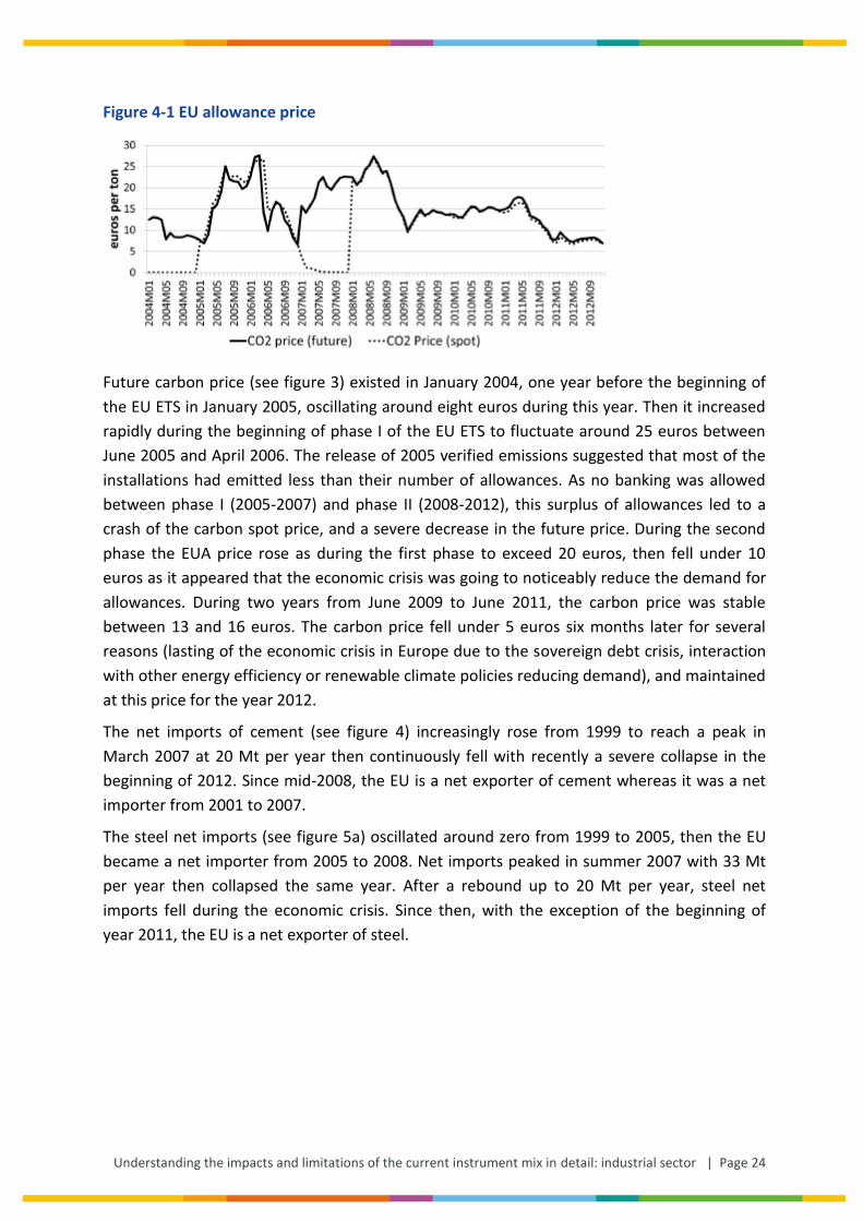
Figure 4-1 EU allowance price
Future carbon price (see figure 3) existed in January 2004, one year before the beginning of
the EU ETS in January 2005, oscillating around eight euros during this year. Then it increased
rapidly during the beginning of phase I of the EU ETS to fluctuate around 25 euros between
June 2005 and April 2006. The release of 2005 verified emissions suggested that most of the
installations had emitted less than their number of allowances. As no banking was allowed
between phase I (2005-2007) and phase II (2008-2012), this surplus of allowances led to a
crash of the carbon spot price, and a severe decrease in the future price. During the second
phase the EUA price rose as during the first phase to exceed 20 euros, then fell under 10
euros as it appeared that the economic crisis was going to noticeably reduce the demand for
allowances. During two years from June 2009 to June 2011, the carbon price was stable
between 13 and 16 euros. The carbon price fell under 5 euros six months later for several
reasons (lasting of the economic crisis in Europe due to the sovereign debt crisis, interaction
with other energy efficiency or renewable climate policies reducing demand), and maintained
at this price for the year 2012.
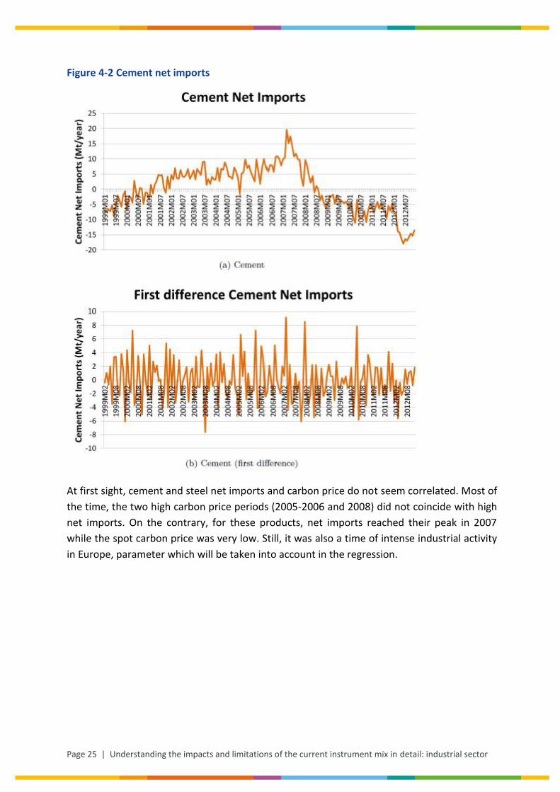
The net imports of cement (see figure 4) increasingly rose from 1999 to reach a peak in
March 2007 at 20 Mt per year then continuously fell with recently a severe collapse in the
beginning of 2012. Since mid-2008, the EU is a net exporter of cement whereas it was a net
importer from 2001 to 2007.
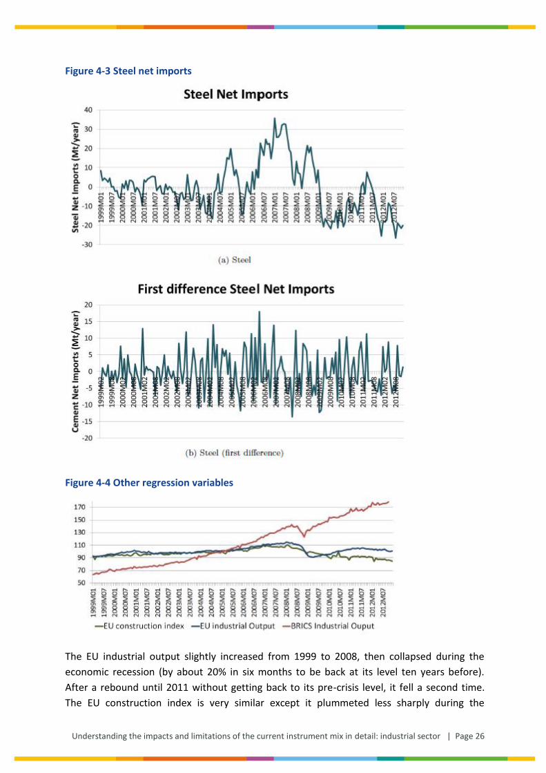
The steel net imports (see figure 5a) oscillated around zero from 1999 to 2005, then the EU
became a net importer from 2005 to 2008. Net imports peaked in summer 2007 with 33 Mt
per year then collapsed the same year. After a rebound up to 20 Mt per year, steel net
imports fell during the economic crisis. Since then, with the exception of the beginning of
year 2011, the EU is a net exporter of steel.
Page 25 | Understanding the impacts and limitations of the current instrument mix in detail: industrial sector
Figure 4-2 Cement net imports
At first sight, cement and steel net imports and carbon price do not seem correlated. Most of
the time, the two high carbon price periods (2005-2006 and 2008) did not coincide with high
net imports. On the contrary, for these products, net imports reached their peak in 2007
while the spot carbon price was very low. Still, it was also a time of intense industrial activity
in Europe, parameter which will be taken into account in the regression.
Understanding the impacts and limitations of the current instrument mix in detail: industrial sector | Page 26
Figure 4-3 Steel net imports
Figure 4-4 Other regression variables
The EU industrial output slightly increased from 1999 to 2008, then collapsed during the
economic recession (by about 20% in six months to be back at its level ten years before).
After a rebound until 2011 without getting back to its pre-crisis level, it fell a second time.
The EU construction index is very similar except it plummeted less sharply during the
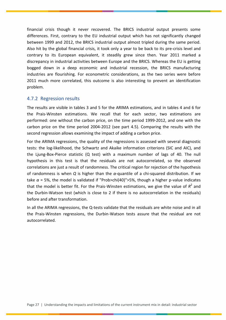
Page 27 | Understanding the impacts and limitations of the current instrument mix in detail: industrial sector
financial crisis though it never recovered. The BRICS industrial output presents some
differences. First, contrary to the EU industrial output which has not significantly changed
between 1999 and 2012, the BRICS industrial output almost tripled during the same period.
Also hit by the global financial crisis, it took only a year to be back to its pre-crisis level and
contrary to its European equivalent, it steadily grew since then. Year 2011 marked a
discrepancy in industrial activities between Europe and the BRICS. Whereas the EU is getting
bogged down in a deep economic and industrial recession, the BRICS manufacturing
industries are flourishing. For econometric considerations, as the two series were before
2011 much more correlated, this outcome is also interesting to prevent an identification
problem.
4.7.2 Regression results
The results are visible in tables 3 and 5 for the ARIMA estimations, and in tables 4 and 6 for
the Prais-Winsten estimations. We recall that for each sector, two estimations are
performed: one without the carbon price, on the time period 1999-2012, and one with the
carbon price on the time period 2004-2012 (see part 4.5). Comparing the results with the
second regression allows examining the impact of adding a carbon price.
For the ARIMA regressions, the quality of the regressions is assessed with several diagnostic
tests: the log-likelihood, the Schwartz and Akaike information criterions (SIC and AIC), and
the Ljung-Box-Pierce statistic (Q test) with a maximum number of lags of 40. The null
hypothesis in this test is that the residuals are not autocorrelated, so the observed
correlations are just a result of randomness. The critical region for rejection of the hypothesis
of randomness is when Q is higher than the α-quantile of a chi-squared distribution. If we
take α = 5%, the model is validated if "Prob>chi(40)">5%, though a higher p-value indicates
that the model is better fit. For the Prais-Winsten estimations, we give the value of R2 and
the Durbin-Watson test (which is close to 2 if there is no autocorrelation in the residuals)
before and after transformation.
In all the ARIMA regressions, the Q-tests validate that the residuals are white noise and in all
the Prais-Winsten regressions, the Durbin-Watson tests assure that the residual are not
autocorrelated.
Understanding the impacts and limitations of the current instrument mix in detail: industrial sector | Page 28
Page 29 | Understanding the impacts and limitations of the current instrument mix in detail: industrial sector
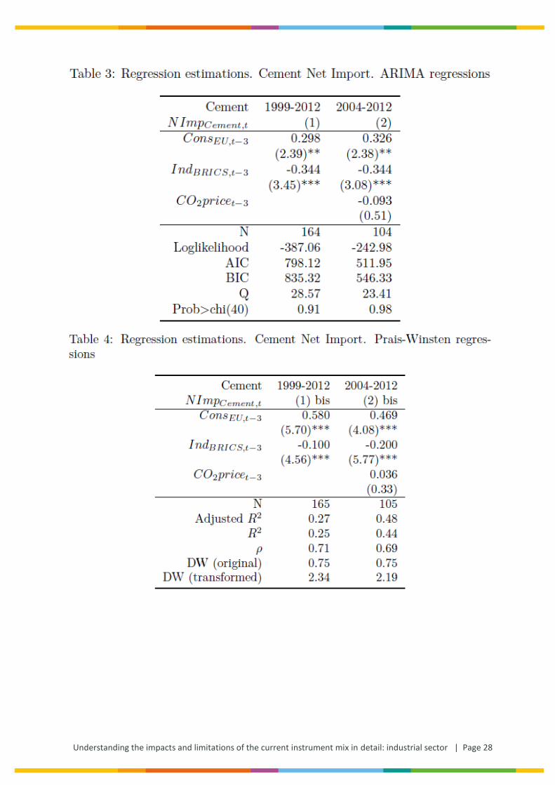
For cement, in regression (1) in table 3, both ConsEU,t−3 and IndBRICS,t−3 are significant,
respectively at the 5% and 1% levels. Hence, we verify that indicators of local and foreign
demand carry explanatory power in cement net imports. Indeed an increase in local demand
is expected to increase the demand for imports and reduce production capacities available
Understanding the impacts and limitations of the current instrument mix in detail: industrial sector | Page 30
for exports. In our model, an increase of 10 points in local demand15 would induce an
increase of about 3 million tonnes of net imports. Besides, we notice that the signs of the
estimated coefficients of ConsEU,t−3 and IndBRICS,t−3 are conform to the theoretical model
(equation (6)). The Ljung-Box-Pierce test validates that the residuals of regression (1) are not
autocorrelated.
The coefficients of ConsEU,t−3 and IndBRICS,t−3 in regression (2) are very similar to the
coefficients of regression (1), and statistically significant respectively at the 10% and 5%
levels. This similarity indicates that the relationship between the cement net imports, local
and foreign demand is robust. CO2pricet−3 is not statistically significant: the carbon price has
no impact on the cement net imports variations. The results of (1)bis and (2)bis in table 4 are
close to the results of (1) and (2), which gives robustness to the results. The coefficients,
except for the carbon price, are all significant at the 1% level.
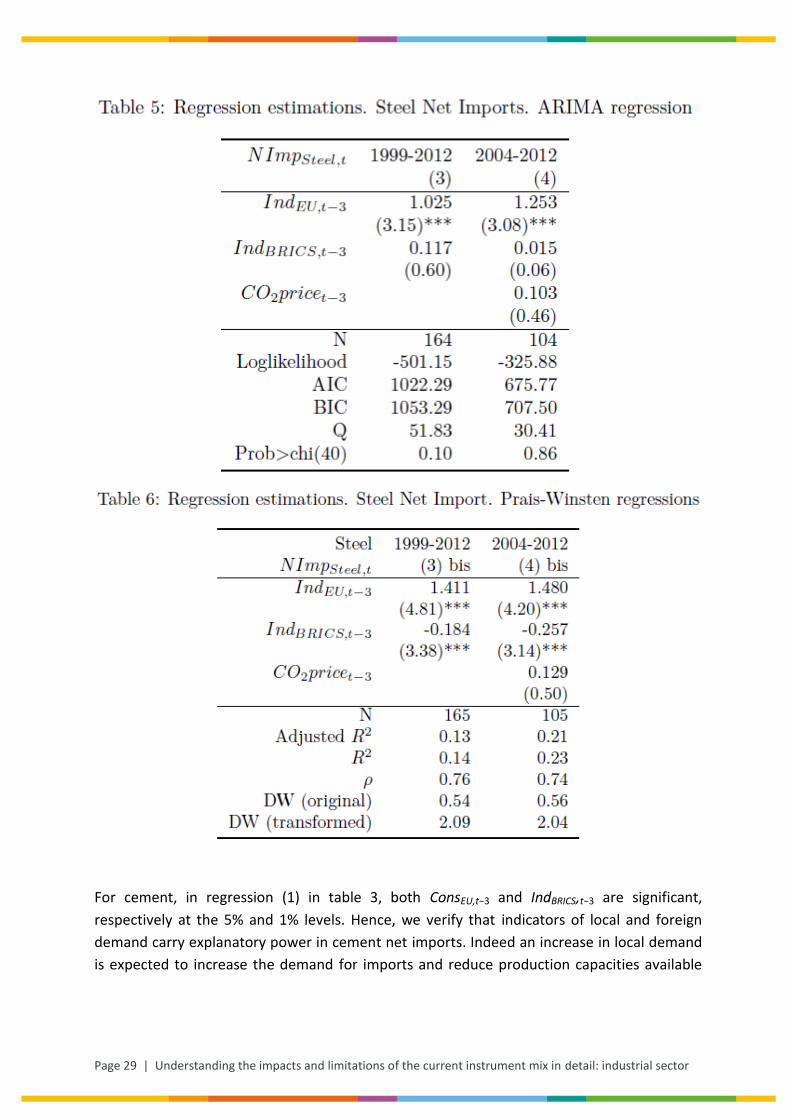
For steel (regression (3) in table 5), IndEU,t−3 is significant at the 1% level, but IndBRICS,t−3 is not
statistically significant; whereas in (3)bis they are both significant at the 1% level. Only the
local demand carries explanatory power in the ARIMA model, while both local and foreign
demands do in the Prais-Winsten estimation. The impact of the local demand is bigger in the
steel industry than in the cement industry16 compared to cement net imports: an increase of
10 points in local demand would lead to an increase of about 9 million tonnes in net imports.
As for cement, the similarity between the results of the two time periods implies that the
relationship between the steel net imports, local and foreign demand is robust. Similarly to
the cement industry, the coefficient of the carbon price CO2pricet−3 is not statistically
significant.
5 Conclusion
Altogether, the work presented in this report points to a simple result: it looks like the EU ETS
has entailed neither what its proponents have hoped for, i.e. significant emissions reduction
(at least in the cement sector), nor what its opponents from the heavy industry side have
feared, i.e. competitiveness losses and carbon leakage (at least in the cement and steel
sectors).
This being said, a few caveat deserve to be mentioned.
First, in the cement sector, the clinker ratio has decreased more rapidly since the start of the
ETS, thereby reducing CO2 emissions. If the clinker ratio had followed its 2000-2005 trend, it
would have been around 2 percentage points higher than its actual value in 2011, resulting in
emissions approximately 2% higher.
15
Demand is normalized to 100 in 2005. 16
Cement net imports are a bit less than twice shorter than steel net imports (see table 2), but the estimated coefficient for local demand (approximated by EU construction or industrial indexes, both around 100) is three times bigger.
Page 31 | Understanding the impacts and limitations of the current instrument mix in detail: industrial sector
Second, there are good reasons to believe that higher abatement occurred in the electricity
sector, where fuel switch and substitutions between power plants of various energy
efficiencies can reduce emissions significantly.
Third, the EU ETS may have contributed to R&D about low-CO2 cements, which can only
deliver in the long run, but the low level of R&D in this sector, as well as the absence of co-
operative R&D programme for low-CO2 cement, comparable to ULCOS17 in the steel sector,
does not invite to optimism.
Fourth, even though the conclusion that no carbon leakage occurred in the short run is
robust, our dataset does not allow us to conclude about long run (‘investment’) leakage, i.e.
an increase in production capacity abroad and a decrease in production capacity in Europe as
the result of EU’s climate policy.
An open question is the role of free allocation in both results. In the first two phases of the
ETS, the allocation rules differed across member states, but in all of them, free allowances
were allocated to new clinker kilns through the new entrant reserve, while closing a clinker
kiln meant sooner or later losing the free allowances. Moreover, grandfathering was the
dominant rule for free allocation, so more allowances (per tonne of capacity) were allocated
for energy-inefficient kilns than for efficient ones.
This means that free allocation provided incentives against abatement (more precisely
against replacing inefficient by efficient kilns), which may contribute to the observed
stagnation of energy efficiency since the start of the ETS. This also means that free allocation
provided an incentive against ‘investment leakage’ i.e. the offshoring of production capacity.
The new allocation rules, applied since the beginning of 2013, correct some of the previous
distortions since a single benchmark applies in all member states and all clinker kilns. This
implies that retrofitting an inefficient plant does not reduce the amount of allowances
received. Yet a potential distortion is constituted by the closure rules which take the form of
activity thresholds: if an installation produce less than 50% of its historic activity level, its
operator loses 50% of its allowances, and 75% of the allowances if it is less than 25%. This
implies that it may be profitable to not close an installation. This generates an incentive, for a
firm operating several plants, to operate all of them at 50% at least, rather than closing the
least efficient plants and operating the others close to their nominal capacity, which could be
the optimal solution without these closure rules (Climate Strategies, 2013).
Ideally, an allowance allocation system in the cement sector would allow mobilising all the
drivers of CO2 abatement while preventing leakage. This is not an easy task since it means
incentivising the replacement of clinker by low-CO2 substitutes but not by clinker imports,
while being compatible with the WTO. Similarly, in the steel sector, it means incentivising a
higher use of scrap but not of steel or pig iron imports. More research is needed to design
such an allowance system.
17
ULCOS stands for Ultra–Low CO2 Steelmaking. It is a consortium of 48 European companies and organisations from 15 European countries that have launched a cooperative research & development initiative. http://www.ulcos.org/en/about_ulcos/home.php

Understanding the impacts and limitations of the current instrument mix in detail: industrial sector | Page 32
Another possible explanation for the low abatement is the volatility of the CO2 price which
clearly hinders the required investments. A price floor system or another device to sustain
the allowance price is clearly required is this respect.
Page 33 | Understanding the impacts and limitations of the current instrument mix in detail: industrial sector
References
Abrell, J., A. Ndoye, and G. Zachmann. Assessing the impact of the EU ETS using firm level data. Bruegel Working
Paper 2011/08, Brussels, Belgium, July 2011.
Aichele, R. and Felbermayr, G. (2012). Kyoto and the carbon footprint of nations. Journal of Environmental
Economics and Management, 63(3):336.
Alberola, E., Chevallier, J., and Chèze, B. (2008). Price drivers and structural breaks in European carbon prices
2005–2007. Energy policy, 36(2):787–797.
Aldy, J. E. and Pizer, W. A. (2011). The competitiveness impacts of climate change mitigation policies. Working
Paper 17705, National Bureau of Economic Research.
Böhringer, C., Balistreri, E. J., and Rutherford, T. F. (2012). The role of border carbon adjustment in unilateral
climate policy: Overview of an energy modeling forum study (EMF 29). Energy Economics, 34:S97–S110.
Branger, F., Lecuyer, O., and Quirion, P. (2013). The European union emissions trading system: should we throw
the flagship out with the bathwater ? CIRED Working Paper 2013-48.
Branger, F. and Quirion, P. (2013a). Climate policy and the ‘carbon haven’ effect. Wiley Interdisciplinary Reviews:
Climate Change, page n/a–n/a.
Branger, F. and Quirion, P. (2013b). Would border carbon adjustment prevent carbon leakage and heavy
industry competitiveness losses? Insights from a meta-analysis of recent economic studies. CIRED Working
Paper 2013-52.
Bredin, D. and Muckley, C. (2011). An emerging equilibrium in the EU emissions trading scheme. Energy
Economics, 33(2):353–362.
Calel, R. and Dechezleprêtre, A. (2012). Environmental policy and directed technological change: evidence from
the European carbon market.
Carbon Trust (2011a). International carbon flows - aluminium. Technical report, Carbon Trust.
Carbon Trust (2011b). International carbon flows - steel. Technical report, Carbon Trust.
Cembureau (2011). Activity Report 2011. Brussels.
Climate Strategies (2013) Carbon Control Post 2020 in Energy Intensive Industries. Learning from the experience
in the cement sector. Energy-Intensive Industries Project Report. Forthcoming, Climate Strategies.
Cochrane, D. and Orcutt, G. H. (1949). Application of least squares regression to relationships containing auto-
correlated error terms. Journal of the American Statistical Association, 44(245):32.
Conrad, C., Rittler, D., and Rotfuß, W. (2012). Modeling and explaining the dynamics of European union
allowance prices at high-frequency. Energy Economics, 34(1):316–326.
Costantini, V. and Mazzanti, M. (2012). On the green and innovative side of trade competitiveness? The impact
of environmental policies and innovation on EU exports. Research Policy, 41(1):132–153.
Understanding the impacts and limitations of the current instrument mix in detail: industrial sector | Page 34
Creti, A., Jouvet, P.-A., and Mignon, V. (2012). Carbon price drivers: Phase I versus phase II equilibrium? Energy
Economics, 34(1):327–334.
CWR (2011). Cement - primer report. Technical report, CarbonWarRoom.
De Bruyn, S., Nelissen, D., and Koopman, M. (2013). Carbon leakage and the future of the EU ETS market. Impact
of recent developments in the EU ETS on the list of sectors deemed to be exposed to carbon leakage.
Technical report, CE Delft, Delft.
Delarue, E., Voorspools, K., and D’haeseleer, W. (2008). Fuel switching in the electricity sector under the EU ETS:
review and prospective. Journal of Energy Engineering, 134(2):40–46.
Demailly, D. and Quirion, P. (2006). CO2 abatement, competitiveness and leakage in the European cement
industry under the EU ETS: grandfathering versus output-based allocation. Climate Policy, 6(1):93–113.
Demailly, D. and Quirion, P. (2008). European emission trading scheme and competitiveness: A case study on
the iron and steel industry. Energy Economics, 30(4):2009–2027.
EAEII (2010). European alliance of energy intensive industries opposes EU unilateral move to -30%. Press
release, European Alliance of Energy Intensive Industries.
Ecofys, W. B. . (2013). Mapping carbon pricing initiatives. Technical report, Ecofys and World Bank.
Ecorys (2008). Study on the competitiveness of the European steel sector. Technical report, Ecorys.
Ederington, J., Levinson, A., and Minier, J. (2003). Footloose and pollution-free. Working Paper 9718, National
Bureau of Economic Research.
Egenhofer et al. (2011) The EU Emissions Trading System and Climate Policy Towards 2050: Real Incentives to
Reduce Emissions and Drive Innovation? Centre for European Policy Studies (CEPS)
Ellerman, A. D., S. M. Feilhauer. 2008. A Top-down and Bottom-up Look at Emissions Abatement in Germany in
Response to the EU ETS. Massachusetts Institute of Technology. Center for Energy, and Environmental Policy
Research. MIT Center for Energy and Environmental Policy Research.
Ellerman, A. D. and Buchner, B. K. (2008). Over-allocation or abatement? A preliminary analysis of the EU ETS
based on the 2005–06 emissions data. Environmental and Resource Economics, 41(2):267–287.
Ellerman, D., Convery, F., and de Perthuis, C. (2010). Pricing Carbon : The European Union Emissions Trading
Scheme. Cambridge, UK, Cambridge university press edition.
Eskeland, G. S. and Harrison, A. E. (2003). Moving to greener pastures? Multinationals and the pollution haven
hypothesis. Journal of Development Economics, 70(1):1–23.
European Commission (2012). The state of the European carbon market in 2012. Technical Report COM(2012)
652, European Commission.
Gerlagh, R. and Kuik, O. (2007). Carbon leakage with international technology spillovers. SSRN Scholarly Paper ID
979915, Social Science Research Network, Rochester, NY.
Gerlagh, R. and Mathys, N. (2011). Energy abundance, trade and industry location. Nota di Lavoro 03-11, FEEM.
Page 35 | Understanding the impacts and limitations of the current instrument mix in detail: industrial sector
Grossman, G. and Krueger, A. (1993). Environmental impact of a north American free trade agreement. In The
Mexico US Free Trade Agreement. Cambridge, Massachusetts, MIT press edition.
Hintermann, B. (2010). Allowance price drivers in the first phase of the EU ETS. Journal of Environmental
Economics and Management, 59(1):43–56.
Holmes, P., Reilly, T., and Rollo, J. (2011). Border carbon adjustments and the potential for protectionism.
Climate Policy, 11(2):883–900.
Hood, C. (2010). Reviewing existing and proposed emissions trading systems. IEA information paper, IEA.
Hourcade, J.-C., Demailly, D., Neuhoff, K., and Sato, M. (2007). Differentiation and dynamics of EU ETS
competitiveness impacts. Technical report, Climate Strategies, Cambridge, UK.
ICR (2012). Global cement report. Technical report, International Cement Review.
Jaffe, A. B., Peterson, S. R., Portney, P. R., and Stavins, R. N. (1995). Environmental regulation and the
competitiveness of US manufacturing: what does the evidence tell us? Journal of Economic literature,
33(1):132–163.
Juergens, I., Barreiro-Hurlé, J., and Vasa, A. (2013). Identifying carbon leakage sectors in the EU ETS and
implications of results. Climate Policy, 13(1):89– 109.
Kalt, J. (1988). The impact of domestic environmental regulatory policies on U.S. international competitiveness.
In International Competitiveness. Ballinger Publishing Company.
Kettner, Claudia, Daniela Kletzan-Slamanig, Angela Köppl. 2013. The EU Emission Trading Scheme – Sectoral
allocation patterns and factors determining emission changes. WIFO Working Papers, No. 444
Kolev, G. I. (2011). The "spurious regression problem" in the classical regression model framework. Economics
Bulletin, 31(1):925–937.
Kuik, O., F. Branger, P. Quirion (2013). International competitiveness and markets. The current policy mix. Report
for the EU FP7 Cecilia2050 project (Task 2.8).
Lacombe, R. (2008). Economic impact of the European Union emissions trading system : Evidence from the
refining sector. MIT master thesis.
Levinson, A. and Taylor, M. S. (2008). Unmasking the pollution haven effect*. International Economic Review,
49(1):223–254.
Mansanet-Bataller, M., Chevallier, J., Hervé-Mignucci, M., and Alberola, E. (2011). EUA and CER phase II price
drivers: Unveiling the reasons for the existence of the EUA–CER spread. Energy Policy, 39(3):1056–1069.
Martin, Ralf, Mirabelle Muûls, Ulrich Wagner. 2012a. An Evidence Review of the EU ETS. DECC. UK.
https://www.gov.uk/government/uploads/system/uploads/attachment_data/file/48449/5725-an-evidence-
review-of-the-eu-emissions-trading-sys.pdf
Martin, R., Muuls, M., de Preux, L., and Wagner, U. (2012b). Industry compensation under relocation risk: A
firm-level analysis of the EU emissions trading scheme. Discussion paper, Center for Economic Performance.
Martínez-Rivera, B. and Ventosa-Santaulària, D. (2012). A comment on ‘Is the spurious regression problem
spurious?’. Economics Letters, 115(2):229–231.
Understanding the impacts and limitations of the current instrument mix in detail: industrial sector | Page 36
McCallum, B. T. (2010). Is the spurious regression problem spurious? Economics Letters, 107(3):321–323.
Meunier, G., Ponssard, J.-P., and Quirion, P. (2012). Carbon leakage and capacity-based allocations: is the EU
right? Working Papers series 4029, CESifo Groups Munich.
Miltner, A. and Salmons, R. (2009). Trends in the competitiveness of selected industrial sectors in ETR countries.
In Carbon-energy Taxation: Lessons from Europe. New York, oxford university press edition.
Neuhoff, Karsten. Tackling Carbon. How to price carbon for climate policy. University of Cambridge. 15/7/2009.
Version 1.2
Oikonomou, V., Patel, M., and Worrell, E. (2006). Climate policy: Bucket or drainer? Energy policy, 34(18):3656–
3668.
Ponssard, J.-P. and Walker, N. (2008). EU emissions trading and the cement sector: a spatial competition
analysis. Climate Policy, 8(5):467–493.
Porter, M. E. and Van der Linde, C. (1995). Toward a new conception of the environment-competitiveness
relationship. The Journal of Economic Perspectives, 9(4):97–118.
Quirion, P. (2011). Les quotas échangeables d’émission de gaz à effet de serre: éléments d’analyse économique.
Mémoire d’HDR, Ecole des Hautes Etudes en Sciences Sociales (EHESS).
Rayner, S. (2010). How to eat an elephant: a bottom-up approach to climate policy. Climate Policy, 10(6):615–
621.
Reinaud, J. (2008a). Climate policy and carbon leakage. impacts of the European emissions trading scheme on
aluminium. IEA information paper, IEA. Reinaud, J. (2008b). Issues behind competitiveness and carbon
leakage. Focus on heavy industries. IEA information paper, International Energy Agency, OECD/IEA Paris.
Sartor, O. (2013). Carbon leakage in the primary aluminium sector: What evidence after 6.5 years of the EU ETS?
SSRN Scholarly Paper ID 2205516, Social Science Research Network, Rochester, NY.
Selim, T. and Salem, A. (2010). Global cement industry: Competitive and institutional dimensions. Technical
Report 24464.
Smarzynska, B. K. (2002). Does foreign direct investment increase the productivity of domestic firms : in search
of spillovers through backward linkages. Policy Research Working Paper Series 2923, The World Bank.
Sollis, R. (2011). Spurious regression: A higher-order problem. Economics Letters, 111(2):141–143.
Tobey, J. A. (1990). The effects of domestic environmental policies on patterns of world trade: An empirical test.
Kyklos, 43(2):191–209.
Ventosa-Santaularia, D. (2012). Unbalanced regressions and spurious inference. Open Journal of Statistics,
02(03):297–299.
WBCSD. 2013. Getting the Numbers Right database. http://wbcsdcement.org/index.php/key-issues/climate-
protection/gnr-database
WCA (2011). Coal and steel facts 2011. Technical report, World Coal Association.
WSA (2012). World steel in figures 2012. Technical Report ISSN 1379-9746, World Steel Association.
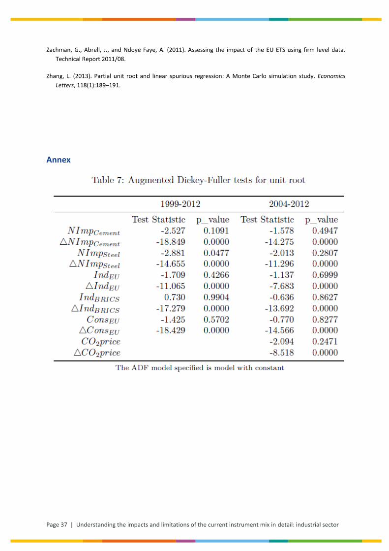
Page 37 | Understanding the impacts and limitations of the current instrument mix in detail: industrial sector
Zachman, G., Abrell, J., and Ndoye Faye, A. (2011). Assessing the impact of the EU ETS using firm level data.
Technical Report 2011/08.
Zhang, L. (2013). Partial unit root and linear spurious regression: A Monte Carlo simulation study. Economics
Letters, 118(1):189–191.
Annex