Journal of Volcanology and Geothermal Research 401 (2020) 106917

Contents lists available at ScienceDirect

Journal of Volcanology and Geothermal Research

j ourna l homepage: www.e lsev ie r .com/ locate / jvo lgeores

Understanding the timing of eruption end using a machine learningapproach to classification of seismic time series

Grace F. Manley a,⁎, David M. Pyle a, Tamsin A. Mather a, Mel Rodgers b, David A. Clifton c, Benjamin G. Stokell d,Glenn Thompsonb, John Makario Londoño e, Diana C. Roman f

a Department of Earth Sciences, University of Oxford, UKb School of Geosciences, University of South Florida, USAc Department of Engineering Science, University of Oxford, UKd Department of Mathematics and Mathematical Statistics, University of Cambridge, UKe Servicio Geológico Colombiano, Observatorio Vulcanológico y Sismológico de Manizales, Colombiaf Department of Terrestrial Magnetism, Carnegie Institution for Science, USA

⁎ Corresponding author.E-mail address: grace.manley@earth.ox.ac.uk (G.F. Ma

https://doi.org/10.1016/j.jvolgeores.2020.1069170377-0273/© 2020 Elsevier B.V. All rights reserved.

a b s t r a c t

a r t i c l e i n f o

Article history:Received 14 November 2019Received in revised form 14 May 2020Accepted 15 May 2020Available online 25 May 2020

The timing and processes that govern the end of volcanic eruptions are not yet fully understood, and there cur-rently exists no systematic definition for the end of a volcanic eruption. Currently, end of eruption is establishedeither by generic criteria (typically 90 days after the end of visual signals of eruption) or criteria specific to a givenvolcano. We explore the application of supervised machine learning classification methods: Support Vector Ma-chine, Logistic Regression, Random Forest and Gaussian Process Classifiers and define a decisiveness index D toevaluate the consistency of the classifications obtained by these models. We apply these methods to seismictime series from two volcanoes chosen because they display contrasting styles of eruption: Telica (Nicaragua)andNevado del Ruiz (Colombia).Wefind that, for both volcanic systems, the end-datewe obtain by classificationof seismic data is 2–4 months later than end-dates defined by the last occurrence of visual eruption (such as ashemission). Thisfinding is in agreementwith previous, general definitions of eruption end and is consistent acrossmodels. Our classifications have a higher correspondence of eruptive activity with visual activity thanwith data-base records of eruption start and end.We analyze the relative importance of the different features of seismic ac-tivity used in our models (e.g. peak event amplitude, daily event counts) and find little consistency between thetwo volcanic systems in terms of the most important features which determine whether activity is eruptive ornon-eruptive. These initial results look promising and our approach may offer a robust tool to help determinewhen an eruption has ended in the absence of visual confirmation.

© 2020 Elsevier B.V. All rights reserved.

1. Introduction

The processes which govern large-scale change in volcanic systemsare not yet fully understood. Volcanic systems are dominated by com-plex and non-linear processes. This complexity has implications forboth understanding and forecasting the onset of volcanic activity (e.g.Sparks, 2003), and for managing transitions in behaviour duringprolonged eruptions (e.g. Sparks and Aspinall, 2004; Hicks and Few,2015; Barclay et al., 2019). While much attention has been focussedon forecasting the timing of eruption onset, and the timing of alerts,warnings and calls for evacuation in the run-up to eruption, or as theeruption escalates (e.g. Marzocchi and Woo, 2007; Winson et al.,2014; Cameron et al., 2018), less attention has been focussed on theends of volcanic eruptions (Bonny and Wright, 2017).

nley).

There is no widely-accepted systematic definition for the end of aneruptive period (e.g. Phillipson et al., 2013) and, as a result, end-datesare often poorly reported. Although some global compilations of volca-nism contain a field for eruption end-date, the end-dates are often notrecorded. The Smithsonian Global Volcanism Program (GVP) highlightthat, of the 10,415 eruptions in the Volcanoes of theWorld (VOTW) da-tabase at the time of writing, there were no available termination datesfor 59% of the entries (Siebert et al., 2011). This lack of data was attrib-uted to the gradual nature of eruption endings, which made assigning adiscrete date difficult. Phillipson et al. (2013) suggest that end-dates inthe GVP database have a temporal uncertainty on the order of days, butinspection of the slow decline in observable activity at some systems(such as Mont Pelée after 1905; or Soufrière Hills Volcano Montserratsince 2010; Lacroix, 1908; Wadge et al., 2014) suggests that the uncer-tainty could be much larger in some cases - not least in the absence of adefinition of what constitutes the ‘end of eruption’. Even in well-monitored cases eruption enddates are hard to determine. For example,

2 G.F. Manley et al. / Journal of Volcanology and Geothermal Research 401 (2020) 106917

even though the activity atMt. St Helens from 2004 to 2008was closelymonitoredwith networks of instruments (including seismic, tilt and gasmeasurements), determining the end of the eruption was impeded bypoor weather conditions throughout the month of December 2007. Itcould not be conclusively determined that small-scale extrusion wasfinished until visual observations were made in January 2008(Dzurisin et al., 2015).

The lack of a specific definition for eruption end has implications forvolcanic hazard. Tilling (2009) cites the mistaken identification of de-creased volcanic activity as the end of eruption as one of the primaryreasons for major loss of life during the 1982 El Chichón eruption. Dela Cruz-Reyna et al. (2017) identify the definition of eruption end as aparticular difficulty during sustained periods of activity, such as at Popo-catépetl in Mexico. Popocatépetl has been in continuous eruption since1994, exhibiting both effusive and explosive activity, butwith lulls in ac-tivity which have led to uncertainty over whether or not they representthe end. Similar stop-start activity has characterised the long-lived andongoing dome-forming eruptions of Santaguito, Guatemala (1922 topresent), and Soufrière Hills Volcano, Montserrat (1995 to present).Better understanding of the timing of eruption end could have implica-tions for the allocation of resources andmanagement of populations liv-ing adjacent to volcanoes during both acute and sustained volcaniceruptions.

Obtaining an operational definition for the end of an eruption relieson piecing together various measurements of volcanic activity to deter-mine when a break in volcanic activity represents the end of the erup-tive period. Definitions for eruption end in a monitoring context comeunder two main categories:

(i) Generic rules on the end of eruptions: For example, Simkin andSiebert (1994) used a generic 90-day (or 3-month) rule for theend of eruption, i.e., that if a volcano displays no visible signs oferuption for 90 days, then the eruption can be considered over;

(ii) Definitions that are volcano-specific. For example, eruptions atPiton de la Fournaise, Réunion, are defined solely on increases ordecreases in seismic tremor amplitude (Battaglia and Aki, 2003).

Volcanic systems undergo periods of activity and repose, on varyingtimescales (e.g. Barmin et al., 2002; Lamb et al., 2014). Identifying thecritical thresholds which govern when large-scale changes in volcanicbehaviour occur is acknowledged as one of the fundamental researchquestions associated with understanding the beginning, evolution andtermination of volcanic activity (NAS, 2017). Development of modelsfor these critical thresholds is necessary to understand the processeswhich drive large-scale change in volcanic behaviour, but this in turnrequires knowing when these changes occur in the timeline of aneruption.

To understand the timing of large-scale change in the system, it isimportant to define the various states of volcanic behaviour. Siebertet al. (2015) define eruption according to the observation of the follow-ing: explosive ejection of either fragmented new magma or older solidmaterial, and/or the effusion of liquid lava. Activity outside eruption isdefined as unrest, and a volcano in no state of eruption or unrest issaid to be in repose (unless extinct). Phillipson et al. (2013) definetwo further categories of unrest: pre-eruptive and non-eruptive unrest,which are based on the presence of observable parameters such as de-formation or seismicity. Neither of these categories can be assigned inreal time, it being necessary to wait either until the crisis has subsidedor an eruption has begun to determine whether the unrest was pre-eruptive or not.

Volcanic state has been previously characterised in models of seis-mic evolution over the eruptive period. McNutt (1996) developed thegeneric earthquake swarm model, which describes the evolution ofseismic activity over an eruptive cycle. In this model, it is suggestedthat the rate and type of seismicity observed over an eruption can begeneralised, and that the physical processes governing the type of

seismicity at each eruptive stage may be inferred. Carniel (2014) de-scribe how time series which have undergone a process of data reduc-tion can be used to identify and infer the timing of transitionsbetween different states of volcanism.

Machine learning is the process by which computers learn withoutbeing explicitly programmed. In fields such as healthcare, jet enginemonitoring or economics, the use of machine learning methods forboth data analysis and real-timemonitoring is already established. Vol-canic systems have conceptual parallels with these systems: they can bedescribed as a “high-integrity” system (Clifton et al., 2014) in which ob-servation of failure (i.e., eruption) is rare in comparison with stable be-haviour, and the number of failure modes are not known or not wellcharacterised. The use of machine learning techniques in volcanologyis an emerging field. Pattern recognition techniques have previouslybeen applied to volcano-seismic data, with a particular focus on detec-tion and classification of seismic event types from raw waveform data(e.g., Langer et al., 2006; Curilem et al., 2009; Apolloni, 2009; Bicegoet al., 2013; Maggi et al., 2017; Malfante et al., 2018). Machine learninghas also been applied to satellite data, in order to detect signs of unrestin large numbers of acquisitions: Anantrasirichai et al. (2018) used deeplearning to detect ground deformation in Sentinel-1 data, and Floweret al. (2016) used logistic regression to detect volcanic eruptions inglobal daily observations of SO2measured using the OzoneMapping In-strument. Ren et al. (2020) usedmulti-station seismic tremor measure-ments to classify behaviour at Piton de la Fournaise volcano and identifyfundamental frequencies of the tremor.

In this paper we use classification machine learning models (seeSection 2.1 for a full description) (i) to classify eruptive and non-eruptive patterns in volcanic time series data, and (ii) to observe howthese patterns differ from inferences based on visual observation or con-ventional monitoring techniques. Similar classification techniques havebeen previously successfully applied in a healthcare context to classifypatient state (e.g., Clifton et al., 2014) and therefore have potential forcharacterising volcanic state. Our approach is distinct from previouswork in volcanology (discussed above) as we classify overall volcanicstate as eruptive or non-eruptive, as opposed to aiming to detect distinctchange in one observable. We present a proof-of-concept study in clas-sifying seismic time series for two volcanoes selected to cover a range oferuptive styles.

2. Methods

2.1. Machine learning methods used

Fig. 1 illustrates the fourmulti-classmethods used for the analysis inthis paper. The methods used are all supervised methods, in which weselect days from time series data (e.g., seismic event counts) for trainingthat include both eruptive and non-eruptive examples to train themodel. During training, some training points are held back and usedto test the trained model to increase the model accuracy (a processknown as model validation). Once a model has been trained, it is thentested using days from the time serieswhichwere not presented duringthe training period.

For this preliminarywork,weusemachine learningmodelswhere fea-tures are calculated and chosen as inputs to themodel, as opposed to othermethods suchasdeep learningwherein features are calculated and chosenwithin themodel. Choosing features asmodel input is preferred so thatwecan use features derived from the seismic data that are similar to thoseused in current monitoring practices. These features, such as event rateor peak signal frequencies, have had widespread success in a monitoringcontext as a basis for distinguishing between states of eruption (Carniel,2014). The established use of these features in a monitoring contextmeans that results such as the relative importance of a given feature inthe models is directly applicable to current observatory practices.

Eachmachine learningmodel we apply is distinct from the others inits method of determining the boundary between non-eruptive and

Fig. 1. Visualisation of how boundaries are defined within the four machine learning methods used in this paper: (a) Support Vector Machine (SVM) (b) Logistic regression (c) Randomforest decision tree (d) Gaussian process classifierwith uncertainty boundsmarked. Red and blue dots denote two classes of data, which in this study represent non-eruptive and eruptivedata. The y-axis in (b) and (d) represents the probability that a given day belongs to the red class or blue class. (For interpretation of the references to color in this figure, the reader isreferred to the web version of this article.)

3G.F. Manley et al. / Journal of Volcanology and Geothermal Research 401 (2020) 106917

eruptive data. We choose to apply multiple methods which have thesame training period, to observe whether the classification of eruptiveand non-eruptive behaviour is consistentwith several distinctmethods.Each method determines the boundary between classes in a differentway, and thus the methods have their own advantages and disadvan-tages. Support Vector Machine models (SVMs, Section 2.1.1) are goodat handling non-linear relationships between data. Logistic regression(LR, Section 2.1.2) is a straightforward model, and thus rarely overfitsdata, while offering a fully interpretable approach whereby its parame-ters are informative of the relative contribution to the classification ofthe input variables. Random forest models (RFs, Section 2.1.3) are gen-erally associated with high classification accuracy and involve taking anensemble of individual decision trees (where the latter are weak classi-fiers). Gaussian Process models (GPs, Section 2.1.4) directly capture theuncertainty associated with the prediction and offer a principled ap-proach to dealing with artefact in time-series data.

2.1.1. Support vector machine (SVMs)SVMs (Fig. 1a) involve finding the hyperplane between two classes

of data which maximises the margin of the classification, where themargin is defined as the perpendicular distance between the decisionboundary and the closest data points (Bishop, 2006). SVMs use the “ker-nel trick” to transform the data to a higher dimensional space, in whichpotential non-linearities in the original data can be separated (whichwould not be possible for logistic regression and other generalised lin-ear models, for example). The choice of kernel depends on the proper-ties of the dataset, such as non-linearity of the data. SVMs have beenwidely used in the field of seismic detection (e.g., Ruano et al., 2014),and they are well suited to general models even with few training ex-amples (Mountrakis et al., 2011). We use the LibSVM libraries (Changand Lin, 2011) to formulate models using both Radial Basis Function(RBF) and even-order polynomial kernels. The values of thehyperparameters for these models are selected using standard 5-foldcross-validation (Hastie et al., 2001).

2.1.2. Logistic regression (LR)LRmodels (Fig. 1b) are a form of generalised linearmodel: thismeans

that the classification linearly depends on the features, where each fea-ture has a coefficient in the linear model. Logistic regression models theposterior probability of a given day being eruptive as a continuous (sig-moid, or S-shaped) function of a linear expression of the features. Theprobabilistic output of these models means that for each day of results,we can infer the certainty of a classification on that day. A full discussionof logistic regression is included in McCullagh and Nelder (1989) andHastie et al. (2001). In the Earth Sciences, LR models have previouslybeen applied in estimation of landslide hazard (Pradhan and Lee, 2010).

2.1.3. Random forest (RF)RF classification (Fig. 1c) involves the averaging of an ensemble of

decision trees: each decision tree comprises a series of operations that

consecutively compare available features in the input data torandomly-selected thresholds on those features (Hastie et al., 2001).Many possible decision trees are combined in random forest classifica-tion: the result of each tree contributes a vote towards the final classifi-cation. The hierarchical nature of decision trees means that thesemethods can be used to determine the relative importance of the fea-tures, where features that appear towards the top of the decision treecontribute more to the classification and are therefore associated withgreater importance (Breiman et al., 1984). Random forest models havebeen applied extensively in remote sensing, due to the high accuracyof classification obtained and their ability to identify important variables(discussed more in Section 4.4; and Belgiu and Drăguţ, 2016).

2.1.4. Gaussian process classification (GPs)Gaussian processes (GPs) (Fig. 1d) fit stochastic models to obtain a

probability that a given data point is in a given class (Bishop, 2006).The classification that results from a Gaussian process classification istherefore associated with a given uncertainty. Like SVMs, GP classifica-tion involves a choice of kernel function to train the model. We use anAutomatic Relevance Determination (ARD) kernel for training models,which allows the importance of each feature input into the model tobe evaluated (Williams and Rasmussen, 2006).

2.2. Model assumptions

The models used in this paper require the fundamental assumptionthat the input variables are Independent and Identically Distributed(IID). Assuming data which are IID implies that each day of features isindependent from other days of features, and that the features oneach day are drawn from the same underlying statistical distribution(Cover and Thomas, 2006). While data are rarely perfectly IID in prac-tice, the assumption typically holds to the degree that models involvingsuch approaches yield satisfactory results. To determinewhether or notthis hypothesis is appropriate for our data, and thereforewhether or notour models can perform well using previously-unseen data, we trainand test (using data held-out during the training process) separatemodels for each volcanic system.

Though we are considering a physical system, which may not pro-vide perfectly IID data, we hypothesise that this assumption is valid toa first order approximation. Other machine learning models existwhich can take into account non-IID behaviour; however, thesemethods are beyond the scope of this paper.

2.3. Nevado del Ruiz and Telica volcanoes

We analyze single-station seismic datasets from two volcanic sys-tems: Nevado del Ruiz Volcano, Colombia and Telica Volcano, Nicaragua.We choose to apply models to the datasets from these two volcanic sys-tems for our test study as they represent contrasting styles of activity.Telica displays near-continuous levels of seismic activity,whereasNevado

4 G.F. Manley et al. / Journal of Volcanology and Geothermal Research 401 (2020) 106917

del Ruiz representsmore punctuated volcanic activity. Therefore, success-ful classification of these differing styles is a useful proof-of-concept thatthese methods have the potential to be extended to a range of volcanicsituations.

Nevado del Ruiz is a stratovolcano in Colombia which primarilyerupts products of andesite-basaltic andesite composition (Cuellar-Rodriguez and Ramirez-Lopez, 1987; Londono, 2016). The dataset isfrom 21st March 2007 to 25th February 2015 and covers two eruptiveperiods, both recorded in GVP. The first phase has a start-date of 22ndFebruary 2012 and end-date of 12th July 2013, and the second, muchshorter, phase has a start-date of 15th December 2014 and end-dateof 7th January 2015. An increase in seismic activity began in September2010 and ash emissions fromNevado del Ruizwere observed from early2012 onwards (Global Volcanism Program, 2017). The 2012 ash emis-sions of Nevado del Ruiz were the first emission of ash since the VEI 3eruption of 1985, which led to the lahar inundation of Armero andN25,000 fatalities (Lowe et al., 1986; Naranjo et al., 1986). The end-date of the first phase is a day later than the last recorded ash emissionand coincideswith the last advisory of theWashingtonVolcanic AshAd-visory Centre (VAAC, 2013). It is unclear how the dates for the secondphase are chosen, as ash emission was observed both in November2014 and later in January 2015.

Telica volcano is a persistently restless volcano in Nicaragua whichundergoes small (VEI 1–2) eruptions every few years (Geirsson et al.,2014; Rodgers et al., 2013; Rodgers et al., 2015a). Persistently restlessvolcanic systems are characterised by high and variable rates of seismic-ity and degassing, with frequent explosive activity (Rodgers et al.,2015a; Geirsson et al., 2014; Roman et al., 2019; Stix, 2007). The Telicadata used for this analysis were obtained from the TESAND network, forthe period 1st April 2010 to 18thMarch 2013. This data period containsone VEI 2 eruption, recorded in GVPwith a start-date of 7thMarch 2011and an end-date of 14th June 2011. The end-date is 3 days after the lastash-and-gas explosion sequence (comprising 17 explosions) was ob-served on 14th June 2011 (Geirsson et al., 2014).

2.4. Classification scheme

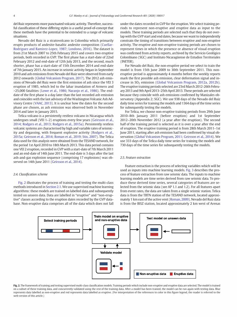
Fig. 2 illustrates the process of training and testing the multi-classmethods introduced in Section 2.1.Weuse supervisedmachine learningalgorithms: thesemodels are trained on labelled data and subsequentlytested on unseen data. Data are labelled in “eruptive” and “non-erup-tive” classes according to the eruption dates recorded by the GVP data-base. Non-eruptive data comprises all of the data which does not fall

Fig. 2. The framework of training and testing supervisedmulti-class classificationmodels. Trainion a subset of these training data, and concurrently validated using the rest of the training drepresents data labelled as non-eruptive and red represents data labelled as eruptive. (For inweb version of this article.)

under the dates recorded in GVP for the eruption.We select training pe-riods to represent non-eruptive and eruptive data as input to themodels. These training periods are selected such that they do not over-lapwith theGVP start and enddates, becausewewant to independentlyconstrain the timing of transitions between eruptive and non-eruptiveactivity. The eruptive and non-eruptive training periods are chosen torepresent times in which the presence or absence of visual eruptionwas confirmed from activity reports, archived by the Servicio GeológicoColombiano (SGC) and Instituto Nicaragüense de Estudios Territoriales(INETER).

For Nevado del Ruiz, the non-eruptive period we select to train themodel is from 15th June 2009 to 30th September 2011. This non-eruptive period is approximately 4 months before the weekly reportsmark the first possible ash emission, clear deformation signal and in-crease in SO2 emission (Global Volcanism Program, 2012a, 2012b).The eruptive training periods selected are 23rdMarch 2012-26th Febru-ary 2013 and 9thApril 2013–25thApril 2013. These periods are selectedbecause they coincide with ash emissions confirmed by Manizales ob-servatory (Appendix 2; SGC). We use 938 days of the Nevado del Ruizdaily time series for training themodels and 1364 days of the time seriesfor subsequently testing the models.

For Telica, we choose non-eruptive training periods from 29th June2010–8th January 2011 (before eruption) and 1st September2012–20th November 2012 (a year after the eruption). The secondhalf of the training period is selected as it is over a year after the endof eruption. The eruptive training period is from 28th March 2011–1stJune 2011, starting after ash emission had been confirmed by visual ob-servation (Global Volcanism Program, 2011; Geirsson et al., 2014). Weuse 333 days of the Telica daily time series for training the models and730 days of the time series for subsequently testing the models.

2.5. Feature extraction

Feature extraction is the process of selecting variables which will beused as inputs into machine learning models. Fig. 3 describes the pro-cess of feature extraction from raw seismic data. The inputs to machinelearning models are time series derived from raw seismic data. To pro-duce these derived time series, several categories of features are se-lected from the seismic data (see AP 1.1 and 1.2). For all features apartfrom event rates, the data are taken from a single seismic station. Telicadata is from the TBTN station of the TESAND network, located approxi-mately 1 kmeast of the active vent (Roman, 2009). Nevado del Ruiz datais from the BISZ station, located approximately 2 km west of Arenas

ngperiodswhich include non-eruptive and eruptive data are selected. Themodel is trainedata. After a model has been trained, the model can be run again with testing data. Blueterpretation of the references to color in this figure legend, the reader is referred to the

Fig. 3. Diagram of the framework for extracting features from raw seismic waveform data. Events are detected from rawwaveform data. From each event waveform we extract featuresincluding the peak amplitudes and band ratio. We then calculate features including the mean and variance from all of the waveforms in a given day. The resulting time series are used asinput for the machine learning model.

5G.F. Manley et al. / Journal of Volcanology and Geothermal Research 401 (2020) 106917

crater (Global Volcanism Program, 2012a, 2012b). For Telica, there are45 features (AP 1.2) and for Nevado del Ruiz (AP 1.1) there are 36 fea-tures in total. There are a greater number of features for Telica due tothe inclusion of features from individual event classifications andRSAM data.

Total event rates per day from network detections are used for bothvolcanoes. For the Telica data, two additional features derive from theautomatic spectral classification of Low Frequency (LF) and High Fre-quency (HF) as defined by Rodgers et al. (2015a). Band ratio is definedas the base 2 log of the ratio of high-frequency to low-frequency energy(Rodgers et al., 2015a; c.f. Buurman andWest, 2010). The distinction be-tween high- and low-frequency bands is dependent on the typical fre-quencies of the volcanic system: for Telica, low-frequency activity isdefined as 1–6 Hz, and high-frequency activity is defined as 6–11 Hz(Rodgers et al., 2015a). Dominant frequencies are obtained by recordingthe 5 peak frequencies from each event during the day. Peak amplitudeis calculated from the maximum peak-peak amplitude of each event.Waveform standard deviation is obtained by calculating the width ofthe largest peakof the spectra for each event during theday. RSAMmea-surements are calculated hourly during the day for the Telica dataset.Multiplet information is the number of waveform families active on agiven day, obtained by waveform cross-correlation using Peakmatch(Rodgers et al., 2015b).

From the categories of observations described above, features arecalculated on a per-day basis by taking the mean, median, variance,minimum, maximum, 10th percentile, 90th percentile and change inmean from the previous day. For multiplets and event rates, only theper-day value and change in value from the previous day is calculated.The RSAM features are mean and variance of the per-hour readingsand change in mean from the previous day. For a full list of featuressee Appendix 1.

For days in the time serieswith zero events, thewhole day is omittedfrom the time series as no features can be extracted for this day. Thegaps in the dataset could be filled using a method such as imputationin which missing data is replaced by a substitute, such as the mean ofthe whole dataset (Schafer and Graham, 2002). However, given thatthe days which have no associated data represent a small proportionof the dataset, we choose to leave these gaps within the time series.

Models can be limited by large quantities of features. High-dimensional systems (those with many features) are not ideal to workwith: as the number of dimensions of data increases, the number oftraining examples required to train a consistent model grows exponen-tially (Bishop, 2006). This phenomenon is known as the “curse of di-mensionality” (Bellman, 1961). For generalised linear models such aslogistic regression, high-dimensional systems are especially poor to

work with (Johnstone and Titterington, 2009). For this reason, weapply regularisation to the logistic regressionmodel, to reduce the num-ber of dimensions as input to the model. We use a technique known asthe Least Absolute Shrinkage and Selection Operator (LASSO) to reducethe number of dimensions as input to the logistic regression models.The LASSO acts to penalise large coefficients in linear models, so that asmaller subset of the full set of features is chosen to model on for eachdataset. A full discussion of the LASSO formulation is included inHastie et al. (2001).

Weuse features derived from single-station seismic data, hence donotinclude derived event parameters such as location or depth. Seismic datais the only type of data which is input to the model. We do not use otherobservables, such as gas or deformation data. The end-date obtained byclassification therefore corresponds to the end of seismicity associatedwith the eruption, and therefore represents the seismic end-date. Seismic-ity can often continue longer than the end of visible eruption, as it reflectsthe processes occurring at depthwithin the volcanic system. Seismic datais one of the most ubiquitous monitoring datasets collected at volcanoesand understanding the path to cessation of processes at depth is crucialin termsof understanding the endof eruptions, supporting the value of fo-cussing only on seismic data for this preliminary study.

The features which we use, with the exception of those associatedwith RSAM, are derived from detected seismic events. The advantageof using these discrete features is that the method could be easily ex-tended to seismic catalog data from other systems with waveforms at-tached. However, depending on the seismic characteristics of a givenvolcano, the inclusion of more features derived from continuous data(such as dominant tremor frequency) may be necessary.

2.6. Eruption classification

Each day in the time series is classified independently from the otherdays. To pick out the large-scale changes in classification, we define arolling threshold filter criterion for a day to be classified as eruptive,which is based on a moving average of the classifications. For a day tobe classified as eruptive, the day itself and the seven days precedingthat day must also be classified as eruptive. By applying this filter tothemodel output, classification of observations as eruptive ismore con-servative than if the results are left unfiltered. The choice to require7 days of eruptive classification is made as the timescale of a week cor-responds to typical timescales on which observations of volcanic activ-ity are communicated to the public where the eruption circumstancesare ongoing or chronic, for example in weekly reports of activity.

6 G.F. Manley et al. / Journal of Volcanology and Geothermal Research 401 (2020) 106917

2.7. Quality assessment: decisiveness index

Our aim when classifying volcanic state is not necessarily to achievemaximum accuracy relative to GVP labels, due to the issue with GVPdefinition of volcanic state (discussed in Section 1).We therefore definean alternative index to model accuracy to evaluate our models. Thisindex is ameasure of how consistent or decisive themodel classificationis over thewhole dataset, expressed as a percentage of the total numberof days containing data. As we are looking to classify overall patterns oferuptive or non-eruptive activity, the decisiveness index favours classi-fications with less noise.

To define the decisiveness index D, we take the number of transi-tions between classes in our models (NtM; where a transition can befromnon-eruptive to eruptive or eruptive to non-eruptive) and subtractthe expected number of transitions corresponding to the number oferuptive periods in the dataset (NtE; where one eruptive period wouldhave two transitions, at the beginning and end of the eruption) thennormalise by the number of days contained within the data period(Nd). An index of 0 means that the number of transitions in the modelare exactly equal to the number of assumed transitions. A larger indexmeans that there is more inconsistency (i.e. more indecision) in thefinal model classification.

D ¼ NtM−NteNd

� 100

The decisiveness index is reported as a percentage. The worst classi-fication which one might produce would alternate between classesevery day, and therefore contain a transition for each day. As the num-ber of days is three orders of magnitude greater than the number oftransitions in the datasets presented here, the number of transitionswould be nearly equal to the total number of days and the decisivenessindex will approach 100%. The decisiveness index is a method to evalu-ate which models make the most consistent classifications of eruptivestate.

The definition of the decisiveness index is a method to evaluatewhich models make the most consistent classifications of eruptivestate. This index makes no assumptions about when the transitionsoccur within the dataset. Therefore, the index is used in conjunctionwith comparison to visual observation of volcanic state in order to eval-uate the success of the models presented within this paper.

3. Results

We independently trained 4 different classification models for eachvolcanic system, with each type of model trained and tested on eachvolcano separately. The analysis could be extended by training amodel on several different seismic datasets, which would be a generalclassification model. However, a general model would require datasets

Table 1Summary of results from all machine learning models applied to the Nevado del Ruiz and Telic

Volcano Method Start-date for firstphase (GVP)

End-date forfirstphase (GVP)

Nevado delRuiz

SVM 22nd February2012

12th July 2013Logistic regressionRandom forestGaussian process classifier(GPC)

Telica SVM 7th March 2011 14th June 2011Logistic regressionRandom forestGaussian process classifier(GPC)

a Decisiveness Index is defined in Section 2.7. Lower D scores are better, and D is comparab

from a greater variety of volcanic settings to ensure that the non-eruptive and eruptive distributions were well-characterised by the ma-chine learning models.

3.1. Nevado del Ruiz

The results from each machine learning method are summarised inTable 1. For all 4 machine learning methods, the end-date of the firstphase of eruption at Nevado del Ruiz obtained by classification of thedata is later than the end-date contained in the GVP database. Fig. 4 il-lustrates the results from the SVM classification of Nevado del Ruizdata in a time series plot for thewhole data period. Several observationscan be made which are consistent features of all of the modelssummarised in Table 1, though we only plot the SVM model (Fig. 4) asit has the highest model accuracy of 82.6% (Table 1):

1. There is a sustained classification of non-eruptive activity before thebeginning of eruptive activity, with only 1 pre-eruptive day errone-ously classified as eruptive in 2007 for the SVM model.

2. The eruption end-date is 4–5 months later than the end-date re-corded in GVP. Though the eruption end-date was recorded as the12th July 2013 just the previous day, active ash emission was ob-served on the 11th July 2013, with further reports of gas and steamemission until November 2013 (Global Volcanism Program, 2017).

3. The second phase of eruption was classified as longer-lived than theGVP start- and end-dates would suggest. Though recorded in GVP ascommencing in December 2014 and finishing in January 2015, theSVM classification of eruptive behaviour lasted from July 2014 toFebruary 2015.Table 1 summarises the results for the decisiveness index when ap-

plied to Nevado del Ruiz. It can be seen that the Gaussian process classi-fier has the best result for the decisiveness index with 3.13%, followedby SVMwith 3.65%. Logistic regression and random forest classificationshave a poorer score for the decisiveness index of 4.78% and 4.17% re-spectively. The range of D for the Nevado del Ruiz models is 1.65%.

Fig. 4 also contains information for the days in the Nevado del Ruizdataset on which there were insufficient data to calculate features.Where there are many data gaps in the sequence, for example, duringnon-eruptive activity in 2007 or during the eruption in mid-2012, theclassification is the same on either side of and during the data gap.From this observation we can determine that the decision to leavedata gaps and not to fill them with a method such as imputation is jus-tified (Section 2.5).

All of the models apart from random forest yield N70% accuracy(where the model result is compared to the GVP label of whether aday is eruptive or non-eruptive) after filtering. The greatest accuracyof 82.6% is achieved by using the SVMmodel. Logistic regressionmodelshave the second highest accuracy (79.6%). High model accuracy istherefore consistent over multiple types of classification, including

a dataset.

Start-date forfirstphase (model)

End-date forfirstphase (model)

Decisivenessindex (%)a

Modelaccuracy(unfiltered)(%)

Modelaccuracy(filtered)(%)

February 2012 November 2013 3.65 76.2 82.6February 2012 December 2013 4.78 75.4 79.6February 2012 November 2013 4.17 62.8 66.9February 2012 November 2013 3.13 67.6 72.7

March 2011 August 2011 3.01 83.6 87.9March 2011 October 2011 3.76 65.1 71.6March 2011 August 2011 3.39 62. 69.5March 2011 August 2011 1.69 86.2 90.5

le across different datasets.

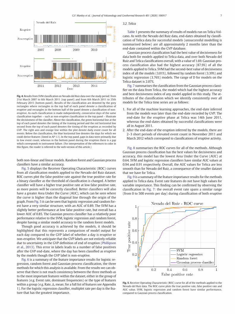
Fig. 4.Results from SVMclassification onNevado del Ruiz data over the study period: from21st March 2007 to 6th March 2011 (top panel) and from 6th March 2011 to 25thFebruary 2015 (bottom panel). Results of the classification are denoted by the greyrectangles where rectangles in the top half of each panel denote a classification oferuptive and rectangles in the bottom half of the panel denote a classification of non-eruptive. As each classification is made independently, consecutive days of the sameclassification together – such as non-eruptive classification in the top panel – illustratethe decisiveness of the classifier. Above the classification, the green horizontal line at thetop of each panel denotes the timing of the training period and the red horizontal linesecond from the top of each panel denotes the timing of the eruption as recorded byGVP. The right axis and orange line within the plot denote daily event count for allevents. Below the classification, the blue horizontal line denotes the days for which wecould derive features (listed in AP 1.1). In the top panel, gaps in data were primarily dueto low event count, whereas in the bottom panel during the eruption there is a gapwhich corresponds to instrument failure. (For interpretation of the references to color inthis figure, the reader is referred to the web version of this article.)

Fig. 5. Receiver Operating Characteristic (ROC) curve for all of the methods applied to theNevado del Ruiz data. The ROC curve plots the true positive rate, false positive rate andAUC value. SVM, logistic regression and random forest have similar performance,compared to Gaussian process classification.

7G.F. Manley et al. / Journal of Volcanology and Geothermal Research 401 (2020) 106917

both non-linear and linearmodels. Random forest and Gaussian processclassifiers have a similar accuracy.

Fig. 5 displays the Receiver Operating Characteristic (ROC) curvesfrom all classification models applied to the Nevado del Ruiz dataset.ROC curves plot the false positive rate against the true positive rate fora binary classifier as the threshold of classification is changed. A betterclassifier will have a higher true positive rate at low false positive rate,as more points will be correctly classified. Better classifiers will alsohave a greater Area Under the Curve (AUC), which can be seen wherethe curve is higher than the diagonal line through the origin of thegraph. From Fig. 5 it can be seen that logistic regression and random for-est have a very similar structure, with an AUC of 0.89. The SVM has aslightly better performance at low false positive rate, but overall has alower AUC of 0.85. The Gaussian process classifier has a relatively poorperformance relative to the SVM, logistic regression and random forest,despite having a similar model accuracy to the random forest models.

Though good accuracy is achieved by the models, it should behighlighted that this represents a comparison of model output foreach day compared to the GVP label of whether a day is eruptive ornon-eruptive. We anticipate that the GVP labels are not entirely reliabledue to uncertainty in the GVP definition of end of eruption (Phillipsonet al., 2013). This error in labels leads to a number of false positivesafter the GVP end-date, where the day has been classified as eruptiveby the models though the GVP label is non-eruptive.

Fig. 6 is a summary of the feature importance results for logistic re-gression, random forest and Gaussian process classification, the threemethods forwhich this analysis is available. From the results we can ob-serve that there is not much consistency between the three methods asto themost important features within the dataset, either in the group offeatures (e.g. Event rate, dominant frequencies) or the type of featureswithin a group (e.g. Rate,Δ, mean; for a full list of features see Appendix1). For the logistic regression classifier, multiplet rate per day is the fea-ture that has the greatest importance.

3.2. Telica

Table 1 presents the summary of results of models run on Telica Vol-cano. As with the Nevado del Ruiz data, end-dates obtained by classifi-cation of Telica data for successful models (unsuccessful modelling issummarised below) are all approximately 2 months later than theend-date contained within the GVP database.

Gaussian process classification had the best value of decisiveness fordata both for models applied to Telica data, and over both Nevado delRuiz and Telica classifications overall, with a value of 1.69. Gaussian pro-cess classification also had the highest accuracy (87.9%) of all themodels applied to Telica. SVMhad the second-best value of decisivenessindex of all the models (3.01%), followed by random forest (3.39%) andlogistic regression (3.76%) models. The range of D for models on theTelica dataset is 2.07%.

Fig. 7 summarises the classification from theGaussian process classi-fier on the data from Telica, the model which had the highest accuracyand best decisiveness index of any model applied in this study. The at-tributes of the classification which we identify consistently over allmodels for the Telica time series are as follows:

1. For all of the machine learning approaches, the end-date inferredfrom the models was later than the end-date recorded by GVP. Theend-date for the eruptive phase at Telica was 14th June 2011,whereas the end-dates obtained by successful classifications wereall in August 2011.

2. After the end-date of the eruption inferred by the models, there are2–3 short periods of elevated event count in November 2011 andMarch 2012 which correspond to classifications of eruptive activity.

Fig. 8 summarises the ROC curves for all of the methods. AlthoughGaussian process classification has the best values for decisiveness andaccuracy, this model has the lowest Area Under the Curve (AUC) at0.64. SVM and logistic regression classifiers have similar AUC values at0.94 and 0.91 respectively. Overall, the AUC values for Telica are lesssmooth than for Nevado del Ruiz, a consequence of the smaller datasetthat we have for Telica.

Fig. 9 is a summary of the feature importance results for themethodsapplied to Telica data. Event rate features do not have high values forvariable importance. This finding can be confirmed by observing theclassification in Fig. 7: the overall event rate spans a similar range(from 0 to 500 events per day) during classification of both eruptive

Fig. 6. Results from feature importance analysis methods on Nevado del Ruiz data. Feature importance is derived from logistic regression (top), random forest (middle) and Gaussianprocess classification (bottom). The y-axis denotes absolute importance which varies depending on the models, normalised by the maximum value for the model. There is a muchgreater range in importance for the Gaussian process classification than for the random forest model. Vertical lines separate the categories of features. For a full list of input featuressee Appendix 1.

8 G.F. Manley et al. / Journal of Volcanology and Geothermal Research 401 (2020) 106917

and non-eruptive activity by ourmodels. As seen for themodels appliedto Nevado del Ruiz, there is not much consistency in the individual fea-tures which are associated with a higher importance.

3.3. Training models with data from the end of volcanic eruption

The Nevado del Ruiz models are trained using two training periods:a period before the beginning of the first eruption and a period duringthe first phase of the eruption (Fig. 4). In these models we do not trainover any transitions between eruptive and non-eruptive behaviour.We now extend the modelling to train over two extra periods usingSVM:

(i) Over the GVP start-date, with training period 23rd June2009–23rd December 2011 (non-eruptive) and 2nd February2012–24th March 2013 (GVP start of eruption).

(ii) Over the GVP end-date, with training period 23rd June2009–23rd September 2011 (non-eruptive) and 29th December2012–26th September 2013 (GVP eruption end).

We would expect the models to successfully classify non-eruptiveand eruptive behaviour if the GVP dates represent reliable labels ofthe transitions in the dataset.

The results from model (i) are very similar to those presented for amodel trained over no transitions in behaviour (Fig. 4). However, for

Fig. 7. Results from GPC classification on Telica data over the study period: from 1st April2010 to 6th October 2011 (top panel) and from 7th October 2011 to 18th March 2012(bottom panel). Results of the classification are denoted by the grey rectangles whererectangles in the top half of each panel denote a classification of eruptive and rectanglesin the bottom half of the panel denote a classification of non-eruptive. As eachclassification is made independently, consecutive days of the same classificationtogether – such as non-eruptive classification in the top panel – illustrate thedecisiveness of the classifier. Above the classification, the green horizontal line at the topof each panel denotes the timing of the training period and the red horizontal linesecond from the top of each panel denotes the timing of the eruption as recorded byGVP. The right axis and yellow line within the plot denote daily event count for allevents. Below the classification, the blue horizontal line denotes the days for which wecould derive features. There are no significant periods of data shortage throughout theTelica data time period. (For interpretation of the references to color in this figure, thereader is referred to the web version of this article.)

Fig. 8. Receiver Operating Characteristic (ROC) curve for all of the methods applied to theTelica data. The ROC curve plots the true positive rate, false positive rate and Area UnderCurve (AUC) value. SVM, logistic regression and random forest have similarperformance, compared to Gaussian process classification.

9G.F. Manley et al. / Journal of Volcanology and Geothermal Research 401 (2020) 106917

model (ii), we obtain a very poor classification: eruptive behaviour isnot classified until July 2012 despite visual evidence of eruption fromFebruary 2012 onwards (Global Volcanism Program, 2012a, 2012b).Moreover, no activity during the second phase of eruption is classifiedas eruptive.We conclude from this result that the eruption end-date re-corded in GVP does not provide a reliable label for the transition be-tween eruptive and non-eruptive behaviour.

4. Discussion

4.1. Classification compared to visual observations

The results presented in Section 3 suggest that in both phases oferuption at Nevado del Ruiz the classification of eruptive activity ismore prolonged than the GVP start- and end-dates would suggest. Apossible reason for the discrepancy between model classification andGVP eruption duration is that GVP classifications are based on visual ob-servation of volcanic activity, whereas we are running models on theseismicity, with 7-day rolling window filtering. Seismicity can indicateprocesses occurring at depths of several kilometres within the volcanicsystem (Moran et al., 2011),which it is reasonable to expectwould con-tinue after visual signals of volcanic eruption had ended. The classifica-tion of eruption until November 2013 (Table 1) could representcontinued or declining seismogenic processes at depth during the de-clining phase of the eruption. In this respect, the seismic end-dates pre-sented here are hypothesised to represent themost generous bound onthe end-date of the eruption.

In Fig. 10 we compare the event rate and model classification tothe alert level recorded at Nevado del Ruiz for the duration of thedata period, as event rate is a commonly-used parameter for inves-tigating volcanic state. The majority of alert level changes wereconcentrated in the period leading up to eruption, and the firstseven months of eruptive activity. There are no alert level changesfollowing 5th September 2012, on which date the alert level was

downgraded from II (Orange) to III (Yellow) (Global VolcanismProgram, 2012a, 2012b). The alert level changes are therefore toocoarse to provide insights into the processes occurring at the endof the eruption.

Fig. 10 also summarises the event rate and recorded ash emissionsaccording to weekly reports and confirmed visual reports of ash emis-sion (Appendix 2; SGC). The classification of the second phase of erup-tive activity precedes the ash emission during July 2014, andcontinues until further ash emission during November 2014. Ourmodel results show a high correlation of eruptive classification withash emission during the second phase of volcanic eruption recordedfrom weekly reports from the Manizales observatory and observatoryrecords (Londono and Galvis, 2018), having trained our model on theseismic signals associated with ash emissions during the first phase ofvolcanic activity.

The good agreement between classification and observation can alsobe noted with a comparison to event rate: though the GVP end-date of11th July 2013 coincides with a consistent low event rate for Nevadodel Ruiz, ourmodel continues to classify behaviour as eruptive for 4 fur-thermonths, which spans a spike in event rate to 1000 events per day inSeptember–October 2011, and culminated in ash emission at the end ofNovember (Global Volcanism Program, 2017).

In the Telica results, we observed deviations between our modelclassification and that of the GVP in terms of end-dates from August–October 2011, in addition to two periods of elevated event rate fromOctober–November 2011 and February–March 2012. These periodsare united by records of “jet-turbine” sounds from the crater initially re-ported by nearby communities (Global Volcanism Program, 2012a,2012b), and by crater incandescence and gas emission in September2011 and February 2012. Overall, comparison to visual observations ismore difficult for Telica data as visual reports of activity are releasedmonthly rather than weekly in Colombia, and there is no system ofalert level classifications.

For both volcanoes, unfiltered models yielded classification of erup-tive activity before the GVP eruption beginning date. However, theseclassifications were not sufficiently consistent to remain as eruptiveafter applying the 7-day rolling filter. Further work is required to seehow these results could be analysed for the case of pre-emptive classifi-cation of eruption to evaluate whether those classifications of eruptiveactivity are truly eruptive or represent a false positive result.

Fig. 9. Results from feature importance analysis methods on Telica data. Feature importance is derived from logistic regression (top), random forest (middle) and Gaussian processclassification (bottom). The y-axis denotes absolute importance which varies depending on the models, normalised by the maximum value for the model. Vertical lines separate thecategories of features.

10 G.F. Manley et al. / Journal of Volcanology and Geothermal Research 401 (2020) 106917

4.2. Possible application of methods and future work

In this study we have shown that retrospective classification of vol-canic activity can yield timing of change with a greater correspondenceto heightened activity and ash emission than end-dates denoted by vi-sual activity judged to be the last of an eruptive phase (Fig. 10). Thecoarseness of alert level changes and the success of the classificationmodel discussed in Section 4.1 presents the possibility to use these ma-chine learning classification methods to identify potential start- andend-dates for seismically monitored volcanoes. Estimates for seismicend of eruption obtained by classification could be combined withother indicators of activity, such as deformation, thermal or gas data,to make a judgement on whether the eruption has ended.

In remote locations, or where conditions are unfavourable for mak-ing visual observations, classification of seismic data could yield a

consistent method for determining transitions in eruptive state in theabsence of other evidence. The work presented here is an example ofhow to distinguish between eruptive and non-eruptive seismic activityusing information from one seismic station alone. For example, thoughno official visual observations of Telica volcano coincidedwith our erup-tive classifications in late 2011 or early 2012, nearby communities re-ported jet-like sounds which coincided with these periods. Furtherapplications for this method could include monitoring volcanoes in re-mote locations where regular visual observations of the volcano arenot practical.

The end-dates yielded by the successful methods are between 2 and4months later than the end-dates judged to be the last visual indicationof eruption (Section 3). Thisfinding is in agreementwith the generic 90-day rule discussed in Section 1. The validation of thismonths-long time-scale of eruption cessation, consistent across volcanoes of differing

Fig. 10. Comparison of the event rate and alert level (top panel) and SVM classification and recorded ash emissions (bottompanel) at Nevado del Ruiz between the dates of 28th June 2010to 25th February 2015. Vertical dashed lines in each plot indicate the GVP start- and end-dates of the twophases of eruption during the data period. Stars indicate confirmed ash emissions.Rectangles in the bottom panel represent the classification from SVM (as in Fig. 4) where blue rectangles are non-eruptive classification and red rectangles are eruptive classification.Wechoose to plot the SVMas itwas the best-performing classifier for Nevado del Ruiz. The alert levelwas consistently green from thebeginning of thedata period to thefirst alert level changeon 30th September 2010. (For interpretation of the references to color in this figure legend, the reader is referred to the web version of this article.)

11G.F. Manley et al. / Journal of Volcanology and Geothermal Research 401 (2020) 106917

eruption style, provides new insights on the physical processes whichgovern changes in seismicity at the end of volcanic eruption. These pro-cesses could include magma withdrawal or relaxation, or rheologicalchanges in the magma (which could in turn be due to, for example, in-creased crystallinity or decreased gas content).

This study is a proof-of-concept of the classification of time series forthe detection of large-scale changes in eruptive systems, and furtherwork would be required to make classifications on a real-time basis. Inaddition, to apply these techniques to a greater number of volcanoes re-quires representative seismic data during eruptive and non-eruptiveperiods to train new models. These models also do not give anyindication of the type or severity of potential eruptive activity whenthe classification is eruptive. Furtherwork, incorporating amore diverserange of time-series observations and datasets into the modelling, isneeded to investigate the sensitivity of the modelled end-dates deter-mination to the nature and variety of datasets used.

The models presented in this study could be extended by defining 3classes for model training and classification. Here, the non-eruptive classcould be split into two classes: one which represents a background classand one which represents a precursory class to eruption. However, tomake this extension it would be necessary to have an independent datastream to reliably distinguish between the background and precursorystates, such as a gas time series hence this analysis is not presented here.

4.3. Failure of logistic regression

For both of the datasets, logistic regression performed poorly rela-tive to the other methods applied to the datasets, with end-dates

1–3 months after the other classification models which were all inagreement. As logistic regression involves linear modelling to definethe classification, failure to characterise the overall volcanic state indi-cates that the underlying relationships are non-linear, even when fea-tures are removed from the dataset through regularisation. Theprocesses governing volcanic eruption have been previously describedas “nonlinear and stochastic” (Sparks, 2003), which could account forthe failure of the logistic regression approach here.

4.4. Feature importance: feature ranking

The feature importance results from the 33methodswhich yield fullfeature importance results are summarised in Fig. 11; here the top 10features ranked as most important in determining the transition be-tween eruptive and non-eruptive for the Nevado del Ruiz and Telicadatasets are plotted. As there may be orders of magnitude betweenthe importance score for these two methods, it is better to value thevery top features. The groups of features with high ranks for bothmethods are dominant frequencies, band ratio and waveform standarddeviation (Nevado del Ruiz), and peak amplitude and dominant fre-quencies (Telica). Dominant frequencies rank in the top 5 features forall methods and for both volcanoes.

Though daily event rate is widely used as a parameter for determin-ing changes in volcanic activity, the daily (total) event rate only appearsin the top 10 features for one method at Nevado del Ruiz, and change inevent rate from the previous day does not appear as a top 10 ranked fea-ture at all. Increases in VT seismicity has been demonstrated as acommon precursor to volcanic eruption at closed volcanic systems,

Fig. 11. Plot of the top 10 ranked features from each feature importance method onNevado del Ruiz (top) and Telica (bottom). Vertical dashed lines represent thedistinction between groups of features (labelled on the x-axis).

12 G.F. Manley et al. / Journal of Volcanology and Geothermal Research 401 (2020) 106917

particularly at previously dormant volcanoes (Cameron et al., 2018).However, studies at basaltic systems including Kilauea Volcano, Hawaii(Chastin andMain, 2003) and Piton de la Fournaise Volcano, Réunion Is-land (Collombet et al., 2003) have found that these precursory increasesin VT seismicity are often either not present, or do not always lead to aneruption. Increases in VT seismicity ending in no eruption have alsobeen documented as “failed eruptions” (Moran et al., 2011),representing a challenge in determining whether a phase of unrestwill lead to eruption. From the results presented here, we cannot con-clusively identify a category of features which distinguishes betweeneruptive and non-eruptive behaviour for both volcanoes.

4.5. Verification of model assumptions

From the successful classification of non-eruptive and eruptive ac-tivity presented in Section 4, we conclude that it is at least approxi-mately correct to make the assumption that the data are Independentand Identically Distributed (IID) for the relatively small VEI and short-lived (b3–5 year) eruptions considered in this study. If similar methodsare applied on different timescales, this assumption may not be valid. Ifdata were binned on a shorter timescale than daily observations, it maynot be appropriate to make this assumption as individual events in cer-tain cases can be quasi-periodic, i.e., not independent from each other(Ignatieva et al., 2018). Following a catastrophic eruption, the assump-tion that each day is drawn from an identical distribution may nothold. Seismicity has been shown to reflect processes within the conduit(e.g., Jousset et al., 2003), which in turn can be eroded by several pro-cesses during eruption including volcanic tremor or wall collapse(Macedonio et al., 1994). Observations of precursory seismic activityat Kelud Volcano, Indonesia preceding the 2007 and 2014 eruptionsfound significant differences in seismic characteristics before both erup-tions, which is consistent with the contrasting eruption dynamics of thetwo events. (Hidayati et al., 2018). Transition periods between eruptiveand non-eruptive data may last on timescales from hours to weeks(Carniel et al., 2003; Ripepe et al., 2002), and behaviour during these

transitions may represent a different mode of the volcanic system(Connor et al., 2003; Rodgers et al., 2016). Though the successfulmodelspresented here indicate that there are no significant transition periodswithin the data periods included in this study, for volcanoes with tran-sition periods on longer timescales (such as days –weeks) the transitionperiod may need to be defined as a separate, third class of activity.

5. Conclusions

Machine learning methods can successfully classify overall patternsof eruptive and non-eruptive behaviour in seismic time series. Thisstudy is the first to apply machine learning techniques to single-station seismic data to classify overall volcanic state as eruptive ornon-eruptive. We define a decisiveness index D to evaluate classifica-tion of eruptive state based on the consistency of classification, whichis comparable across datasets. Our models have a high agreement interms of eruptive classification with visual indicators of eruption, suchas ash emissions. Thedate of the eruption end is found to be consistentlylater than the date recorded inGVP, by approximately 60–120 days. Thisfinding is in agreementwith previous, non-physical definitions of end ofvolcanic eruption, such as the 90-day rule for determining the timing oferuption end (Simkin and Siebert, 1994). Classification of eruptive andnon-eruptive data could be applied to seismic time series to determinewhen end of eruption occurred, in the absence of conclusive visual ob-servations. Support Vector Machine and Gaussian Process Classifierswere the most successful classification models applied to Nevado delRuiz and Telica respectively. Logistic regression, a linear classifier, hadlower classification accuracy and decisiveness for both datasets, whichcould be due to non-linearity in the data. Feature importance methodsidentified little consistency between the most important seismic fea-tures used as model inputs. Work on a larger number and variety ofdatasets is necessary to determine whether these most important fea-tures are consistent between volcanoes, or between volcanoes withsimilar eruption styles or tectonic settings.

CRediT authorship contribution statement

Grace F. Manley: Conceptualization, Investigation, Formal analysis,Writing - original draft, Writing - review & editing. DavidM. Pyle: Con-ceptualization, Supervision, Writing - review & editing. Tamsin A.Mather: Conceptualization, Supervision, Writing - review & editing.Mel Rodgers: Conceptualization, Data curation, Supervision, Writing -review & editing. David A. Clifton: Conceptualization, Supervision,Writing - review & editing. Benjamin G. Stokell:Data curation,Writing- review & editing. Glenn Thompson:Writing - review & editing. JohnMakario Londoño: Data curation, Writing - review & editing. Diana C.Roman:Writing - review & editing.

Declaration of competing interest

The authors declare that they have no known competing financialinterests or personal relationships that could have appeared to influ-ence the work reported in this paper.

Acknowledgements and data statement

Telica data was collected by the TESAND network (NSF EAR-0911366 to D. Roman and P. LaFemina). Nevado del Ruiz data was ob-tained from theObservatorio Vulcanológico y Sismológico deManizales,Servicio Geológico Colombiano. This research has been supported by aNatural Environment Research Council(NERC) studentship (NE/L002612/1). Contributions to the work were facilitated by a NERC Re-search Experience Placement to the British Geological Survey. Matherand Pyle acknowledge support from NERC/ESRC grants NE/J020001/1and NE/J020052/1 (STREVA). Two anonymous reviewers are thankedfor their helpful comments on an earlier version of the paper.

13G.F. Manley et al. / Journal of Volcanology and Geothermal Research 401 (2020) 106917

Appendix A. Supplementary data

Supplementary data to this article can be found online at https://doi.org/10.1016/j.jvolgeores.2020.106917.

References

Anantrasirichai, N., Biggs, J., Albino, F., Hill, P., Bull, D., 2018. Application of machine learn-ing to classification of volcanic deformation in routinely generated InSAR data.J. Geophys. Res. Solid Earth 123 (8), 6592–6606.

Apolloni, B., 2009. Support vector machines and MLP for automatic classification of seis-mic signals at Stromboli volcano. Neural Nets WIRN09: Proceedings of the 19th Ital-ian Workshop on Neural Nets, Vietri Sul Mare, Salerno, Italy May 28–30 2009. 204.IOS Press, p. 116.

Barclay, J., Few, F., Armijos, M.T., Phillips, J.C., Pyle, D.M., Hicks, A.J., Brown, S.K., Robertson,R.E.A., 2019. Livelihoods, wellbeing and the risk to life during volcanic eruptions.Front. Earth Sci. 7, 205. https://doi.org/10.3389/feart.2019.00205.

Barmin, A., Melnik, O., Sparks, R.S.J., 2002. Periodic behavior in lava dome eruptions. EarthPlanet. Sci. Lett. 199 (1), 173–184.

Battaglia, J., Aki, K., 2003. Location of seismic events and eruptive fissures on the Piton dela Fournaise volcano using seismic amplitudes. J. Geophys. Res. Solid Earth 108 (B8),2364. https://doi.org/10.1029/2002JB002193.

Belgiu, M., Drăguţ, L., 2016. Random forest in remote sensing: a review of applications andfuture directions. ISPRS J. Photogramm. Remote Sens. 114, 24–31.

Bellman, R.E., 1961. Adaptive Control Processes: A Guided Tour. Princeton UniversityPress, Princeton, New Jersey, USA.

Bicego, M., Acosta-Muñoz, C., Orozco-Alzate, M., 2013. Classification of seismic volcanicsignals using hidden-Markov-model-based generative embeddings. IEEE Trans.Geosci. Remote Sens. 51 (6), 3400–3409.

Bishop, C.M., 2006. Pattern Recognition and Machine Learning. Springer, New York.Bonny, E., Wright, R., 2017. Predicting the end of lava flow-forming eruptions from space.

Bull. Volcanol. 79 (7), 52. https://doi.org/10.1007/s00445-017-1134-8.Breiman, L., Friedman, R.A., Olshen, R.A., Stone, C.G., 1984. Classification and Regression

Trees. Wadsworth, Pacific Grove, CA.Buurman, H., West, M., 2010. Seismic precursors to volcanic explosions during the 2006

eruption of Augustine Volcano. In: Power, J., Coombs, M., Freymueller, J. (Eds.), The2006 Eruption of Augustine Volcano. U.S. Geological Survey Professional Paper1769, Alaska (U.S. Geological Survey Professional Paper 1769).

Cameron, C.E., Prejean, S.G., Coombs, M.L., Wallace, K.L., Power, J.A., Roman, D.C., 2018.Alaska volcano observatory alert and forecasting timeliness: 1989–2017. Front.Earth Sci. 6, 86. https://doi.org/10.3389/feart.2018.00086.

Carniel, R., 2014. Characterization of volcanic regimes and identification of significanttransitions using geophysical data: a review. Bull. Volcanol. 76 (8), 848. https://doi.org/10.1007/s00445-014-0848-0.

Carniel, R., Di Cecca, M., Rouland, D., 2003. Ambrym, Vanuatu (July–August 2000): spec-tral and dynamical transitions on the hours-to-days timescale. J. Volcanol. Geotherm.Res. 128 (1–3), 1–13.

Chang, C.C., Lin, C.J., 2011. LIBSVM: a library for support vector machines. ACM Trans.Intell. Syst. Technol. (TIST) 2 (3), 27.

Chastin, S.F., Main, I.G., 2003. Statistical analysis of daily seismic event rate as a precursor tovolcanic eruptions. Geophys. Res. Lett. 30 (13). https://doi.org/10.1029/2003GL016900.

Clifton, L., Clifton, D.A., Pimentel, M.A.F., Watkinson, P.J., Tarassenko, L., 2014. Predictivemonitoring of mobile patients by combining clinical observations with data fromwearable sensors. IEEE J. Biomed. Health Inform. 18 (3), 722–730 2014.

Collombet, M., Grasso, J.R., Ferrazzini, V., 2003. Seismicity rate before eruptions on Pitonde la Fournaise volcano: Implications for eruption dynamics. Geophys. Res. Lett. 30(21), 2099. https://doi.org/10.1029/2003GL017494.

Connor, C.B., Sparks, R.S.J., Mason, R.M., Bonadonna, C., Young, S.R., 2003. Exploring linksbetween physical and probabilistic models of volcanic eruptions: the Soufriere HillsVolcano, Montserrat. Geophys. Res. Lett. 30 (13).

Cover, T.M., Thomas, J.A., 2006. Elements of Information Theory. 2nd edition. Wiley-Interscience, NJ.

Cuellar-Rodriguez, J.V., Ramirez-Lopez, C., 1987. Descripcion de los volcanes Colombianos.Rev CIAF, Bogota, pp. 189–222.

Curilem, G., Vergara, J., Fuentealba, G., Acuña, G., Chacón, M., 2009. Classification of seis-mic signals at Villarrica volcano (Chile) using neural networks and genetic algo-rithms. J. Volcanol. Geotherm. Res. 180 (1), 1–8.

De la Cruz-Reyna, S., Tilling, R.I., Valdés-González, C., 2017. Challenges in Responding to aSustained, Continuing Volcanic Crisis: The Case of Popocatepétl Volcano, Mexico,1994–Present.

Dzurisin, D., Moran, S.C., Lisowski, M., Schilling, S.P., Anderson, K.R., Werner, C., 2015. The2004–2008 dome-building eruption at Mount St. Helens, Washington: epilogue. Bull.Volcanol. 77 (17). https://doi.org/10.1007/s00445-015-0973-4.

Flower, V.J., Oommen, T., Carn, S.A., 2016. Improving global detection of volcanic erup-tions using the ozone monitoring Instrument (OMI). Atmos. Measurement Tech-niques 9 (11), 5487–5498.

Geirsson, H., Rodgers, M., LaFemina, P., Witter, M., Roman, D., Muñoz, A., Tenorio, V.,Alvarez, J., Jacobo, V.C., Nilsson, D., Galle, B., 2014. Multidisciplinary observations ofthe 2011 explosive eruption of Telica volcano, Nicaragua: implications for the dy-namics of low-explosivity ash eruptions. J. Volcanol. Geotherm. Res. 271, 55–69.

Global Volcanism Program, 2011. Report on Telica (Nicaragua). In: Sennert, S.K. (Ed.),Weekly Volcanic Activity Report, 11 May–17 May 2011. Smithsonian Institutionand US Geological Survey.

Global Volcanism Program, 2012a. Report on Nevado del Ruiz (Colombia). In: Sennert,S.K. (Ed.), Weekly Volcanic Activity Report, 7 March–13March 2012. Smithsonian In-stitution and US Geological Survey.

Global Volcanism Program, 2012b. Report on Telica (Nicaragua). In: Sennert, S.K. (Ed.),Weekly Volcanic Activity Report, 12 September–18 September 2012. Smithsonian In-stitution and US Geological Survey.

Global Volcanism Program, 2017. Report on Nevado del Ruiz (Colombia). In: Venzke, E.(Ed.), Bulletin of the Global Volcanism Network. 42. Smithsonian Institution, p. 6.

Hastie, T., Tibshirani, R., Friedman, J., 2001. The Elements of Statistical Learning. Springer,New York. NY.

Hicks, A., Few, R., 2015. Trajectories of social vulnerability during the Soufrière Hills vol-canic crisis. J. Appl. Volcanol. 4, 10. https://doi.org/10.1186/s13617-015-0029-7.

Hidayati, S., Triastuty, H., Mulyana, I., Adi, S., Ishihara, K., Basuki, A., Kuswandarto, H.,Priyanto, B., Solikhin, A., 2018. Differences in the seismicity preceding the 2007 and2014 eruptions of Kelud volcano, Indonesia. J. Volcanol. Geotherm. Res. 382, 50–67.https://doi.org/10.1016/j.jvolgeores.2018.10.017.

Ignatieva, A., Bell, A., Worton, B., 2018. Point process models for quasi-periodic volcanicearthquakes. Stat. Volcanol. 4. https://doi.org/10.5038/2163-338X.4.2.

Johnstone, I.M., Titterington, D.M., 2009. Statistical challenges of high-dimensional data.Phil. Trans. R. Soc. A 367. https://doi.org/10.1098/rsta.2009.0159.

Jousset, P., Neuberg, J., Sturton, S., 2003. Modelling the time-dependent frequency contentof low-frequency volcanic earthquakes. J. Volcanol. Geotherm. Res. 128 (1–3),201–223.

Lacroix, A., 1908. La montagne Pelée après ses éruptions, avec observations sur les érup-tions du Vésuve en 79 et en 1906. Masson et cie.

Lamb, O.D., Varley, N.R., Mather, T.A., Pyle, D.M., Smith, P.J., Liu, E.J., 2014. Multiple time-scales of cyclical behaviour observed at two dome-forming eruptions. J. Volcanol.Geotherm. Res. 284, 106–121.

Langer, H., Falsaperla, S., Powell, T., Thompson, G., 2006. Automatic classification and a-posteriori analysis of seismic event identification at Soufriere Hills volcano, Montser-rat. J. Volcanol. Geotherm. Res. 153 (1–2), 1–10.

Londono, J.M., 2016. Evidence of recent deep magmatic activity at Cerro Bravo-CerroMachín volcanic complex, central Colombia. Implications for future volcanic activityat Nevado del Ruiz, Cerro Machín and other volcanoes. J. Volcanol. Geotherm. Res.324, 156–168.

Londono, J.M., Galvis, B., 2018. Seismic data, photographic images and physical modelingof volcanic plumes as a tool for monitoring the activity of Nevado del Ruiz Volcano,Colombia. Front. Earth Sci. 6, 162. https://doi.org/10.3389/feart.2018.00162.

Lowe, D.R., Williams, S.N., Leigh, H., Connor, C.B., Gemmell, J.B., Stoiber, R.E., 1986. Laharsinitiated by the 13 November 1985 eruption of Nevado del Ruiz, Colombia. Nature324 (6092), 51.

Macedonio, G., Dobran, F., Neri, A., 1994. Erosion processes in volcanic conduits and appli-cation to the AD 79 eruption of Vesuvius. Earth Planet. Sci. Lett. 121 (1–2), 137–152.

Maggi, A., Ferrazzini, V., Hibert, C., Beauducel, F., Boissier, P., Amemoutou, A., 2017. Imple-mentation of a multistation approach for automated event classification at Piton de laFournaise volcano. Seismol. Res. Lett. 88 (3), 878–891.

Malfante, M., Dalla Mura, M., Mars, J.I., Métaxian, J.P., Macedo, O., Inza, A., 2018. Automaticclassification of volcano seismic signatures. J. Geophys. Res. Solid Earth 123 (12),10–645.

Marzocchi, W., Woo, G., 2007. Probabilistic eruption forecasting and the call for an evac-uation. Geophys. Res. Lett. 34, 22.

McCullagh, P., Nelder, J.A., 1989. Generalized Linear Models. 37. CRC press.McNutt, S.R., 1996. Seismic monitoring and eruption forecasting of volcanoes: a review of

the state-of-the-art and case histories. Monitoring andMitigation of Volcano Hazards.Springer, Berlin, Heidelberg, pp. 99–146.

Moran, S.C., Newhall, C., Roman, D.C., 2011. Failed magmatic eruptions: late-stage cessa-tion of magma ascent. Bull. Volcanol. 73 (2), 115–122.

Mountrakis, G., Im, J., Ogole, C., 2011. Support vector machines in remote sensing: a re-view. ISPRS J. Photogramm. Remote Sens. 66 (3), 247–259.

Naranjo, J.L., Sigurdsson, H., Carey, S.N., Fritz, W., 1986. Eruption of the Nevado del Ruizvolcano, Colombia, on 13 November 1985: tephra fall and lahars. Science 233(4767), 961–963.

National Academies of Sciences, Engineering, and Medicine, 2017. Volcanic Eruptions andTheir Repose, Unrest, Precursors, and Timing. The National Academies Press,Washington, DC https://doi.org/10.17226/24650.

Phillipson, G., Sobradelo, R., Gottsmann, J., 2013. Global volcanic unrest in the 21st cen-tury: an analysis of the first decade. J. Volcanol. Geotherm. Res. 264, 183–196.

Pradhan, B., Lee, S., 2010. Landslide susceptibility assessment and factor effect analysis:backpropagation artificial neural networks and their comparison with frequencyratio and bivariate logistic regression modelling. Environ. Model Softw. 25 (6),747–759.

Ren, C.X., Peltier, A., Ferrazzini, V., Rouet-Leduc, B., Johnson, P.A., Brenguier, F., 2020. Ma-chine learning reveals the seismic signature of eruptive behavior at piton de lafournaise volcano. Geophys. Res. Lett. 47 (3), e2019GL085523. https://doi.org/10.1029/2019GL085523.

Ripepe, M., Harris, A.J., Carniel, R., 2002. Thermal, seismic and infrasonic evidences of var-iable degassing rates at Stromboli volcano. J. Volcanol. Geotherm. Res. 118 (3–4),285–297.

Rodgers, M., Roman, D.C., Geirsson, H., LaFemina, P., Muñoz, A., Guzman, C., Tenorio, V.,2013. Seismicity accompanying the 1999 eruptive episode at Telica Volcano,Nicaragua. J. Volcanol. Geotherm. Res. 265, 39–51.

Rodgers, M., Roman, D.C., Geirsson, H., LaFemina, P., McNutt, S.R., Muñoz, A., Tenorio, V.,2015a. Stable and unstable phases of elevated seismic activity at the persistently rest-less Telica Volcano, Nicaragua. J. Volcanol. Geotherm. Res. 290, 63–74.

Rodgers, M., Rodgers, S., Roman, D.C., 2015b. Peakmatch: a Java program for multipletanalysis of large seismic datasets. Seismol. Res. Lett. 86 (4), 1208–1218.

14 G.F. Manley et al. / Journal of Volcanology and Geothermal Research 401 (2020) 106917

Rodgers, M., Smith, P.J., Mather, T.A., Pyle, D.M., 2016. Quiescent-explosive transitionsduring dome-forming volcanic eruptions: using seismicity to probe the volcanic pro-cesses leading to the 29 July 2008 Vulcanian explosion of Soufrière Hills Volcano,Montserrat. J. Geophys. Res. Solid Earth 121 (12), 8453–8471.

Roman, D.C., 2009. Telica Seismic and Deformation Network. International Federation ofDigital Seismograph Networks https://doi.org/10.7914/SN/6D_2009.

Roman, D.C., LaFemina, P.C., Bussard, R., Stephens, K., Wauthier, C., Higgins, M., et al.,2019. Mechanisms of unrest and eruption at persistently restless volcanoes: Insightsfrom the 2015 eruption of Telica Volcano, Nicaragua. Geochem. Geophys. Geosyst., 20https://doi.org/10.1029/2019GC008450.

Ruano, A.E., Madureira, G., Barros, O., Khosravani, H.R., Ruano, M.G., Ferreira, P.M., 2014.Seismic detection using support vector machines. Neurocomputing 135, 273–283.

Schafer, J.L., Graham, J.W., 2002. Missing data: our view of the state of the art. Psychol.Methods 7 (2), 147.

Siebert, L., Simkin, T., Kimberly, P., 2011. Volcanoes of the World. Univ of California Press.Siebert, L., Cottrell, E., Venzke, E., Andrews, B., 2015. Earth’s volcanoes and their eruptions:

An overview. The Encyclopedia of Volcanoes. Academic Press, pp. 239–255.Simkin, T., Siebert, L., 1994. Volcanoes of the World. Geosciences Press, Inc, Tusson.

Sparks, R.S.J., 2003. Forecasting volcanic eruptions. Earth Planet. Sci. Lett. 210 (1–2), 1–15.Sparks, R.S.J., Aspinall, W., 2004. Volcanic activity: frontiers and challenges in forecasting,

prediction and risk assessment. Geophys. Monogr. 150, 359–373.Stix, J., 2007. Stability and instability of quiescently active volcanoes: the case of Masaya,

Nicaragua. Geology 35 (6), 535–538.Tilling, R.I., 2009. El Chichón’s“ surprise” eruption in 1982: Lessons for reducing volcano

risk. Geofis. Int. 48 (1), 3–19.VAAC, 2013. Washington VAAC 2013 Volcano Ash Advisory Archive. Satellite Products

and Services Division/Office of Satellite and Product Operations,Washington VolcanicAsh Advisory Centre https://www.ssd.noaa.gov/VAAC/ARCH13/archive.html.

Wadge, G., Voight, B., Sparks, R.S.J., Cole, P.D., Loughlin, S.C., Robertson, R.E.A., 2014. Anoverview of the eruption of Soufriere Hills Volcano, Montserrat from 2000 to 2010.Geol. Soc. Lond. Mem. 39 (1), 1–40.

Williams, C.K., Rasmussen, C.E., 2006. Gaussian Processes for Machine Learning (Vol. 2,No. 3, p. 4). MIT Press, Cambridge, MA.

Winson, A.E., Costa, F., Newhall, C.G., Woo, G., 2014. An analysis of the issuance of volcanicalert levels during volcanic crises. J. Appl. Volcanol. 3 (1), 14.