understanding type ia supernovae through their u ... - arxiv · 2 physics division, lawrence...

Astronomy & Astrophysics manuscript no. ms c©ESO 2018January 8, 2018

Understanding Type Ia supernovae through their U-band spectraJ. Nordin1, G. Aldering2, P. Antilogus3, C. Aragon2, S. Bailey2, C. Baltay4, K. Barbary2, 5, S. Bongard3, K. Boone2, 6,V. Brinnel1, C. Buton7, M. Childress8, N. Chotard7, Y. Copin7, S. Dixon2, P. Fagrelius2, 6, U. Feindt9, D. Fouchez10,E. Gangler11, B. Hayden2, W. Hillebrandt12, A. Kim2, M. Kowalski1, 13, D. Kuesters1, P.-F. Leget,11, S. Lombardo1,

Q. Lin14, R. Pain3, E. Pecontal15, R. Pereira7, S. Perlmutter2, 6, D. Rabinowitz4, M. Rigault1, K. Runge2, D. Rubin2, 16,C. Saunders2, 3, G. Smadja7, C. Sofiatti2, 6, N. Suzuki2, 19, S. Taubenberger12, 17, C. Tao10, 14, and R. C. Thomas18

The Nearby Supernova Factory

1 Institut fur Physik, Humboldt-Universitat zu Berlin, Newtonstr. 15, 12489 Berlin2 Physics Division, Lawrence Berkeley National Laboratory, 1 Cyclotron Road, Berkeley, CA, 947203 Laboratoire de Physique Nucléaire et des Hautes Énergies, Université Pierre et Marie Curie Paris 6, Université Paris Diderot Paris

7, CNRS-IN2P3, 4 place Jussieu, 75252 Paris Cedex 05, France4 Department of Physics, Yale University, New Haven, CT, 06250-81215 Berkeley Center for Cosmological Physics, University of California Berkeley, Berkeley, CA, 947206 Department of Physics, University of California Berkeley, 366 LeConte Hall MC 7300, Berkeley, CA, 94720-73007 Université de Lyon, F-69622, Lyon, France ; Université de Lyon 1, Villeurbanne ; CNRS/IN2P3, Institut de Physique Nucléaire

de Lyon.8 Department of Physics and Astronomy, University of Southampton, Southampton, Hampshire, SO17 1BJ, UK9 The Oskar Klein Centre, Department of Physics, AlbaNova, Stockholm University, SE-106 91 Stockholm, Sweden

10 Aix Marseille Université, CNRS/IN2P3, CPPM UMR 7346, 13288, Marseille, France11 Clermont Université, Université Blaise Pascal, CNRS/IN2P3, Laboratoire de Physique Corpusculaire, BP 10448, F-63000

Clermont-Ferrand, France12 Max-Planck Institut für Astrophysik, Karl-Schwarzschild-Str. 1, 85748 Garching, Germany13 Deutsches Elektronen-Synchrotron, D-15735 Zeuthen, Germany14 Tsinghua Center for Astrophysics, Tsinghua University, Beijing 100084, China15 Centre de Recherche Astronomique de Lyon, Université Lyon 1, 9 Avenue Charles André, 69561 Saint Genis Laval Cedex, France

16 Space Telescope Science Institute, 3700 San Martin Drive, Baltimore, MD 2121817 European Southern Observatory, Karl-Schwarzschild-Str. 2, 85748 Garching, Germany18 Computational Cosmology Center, Computational Research Division, Lawrence Berkeley National Laboratory, 1 Cyclotron Road

MS 50B-4206, Berkeley, CA, 9472019 Kavli Institute for the Physics and Mathematics of the Universe, University of Tokyo, 5-1-5 Kashiwanoha, Kashiwa, Chiba, 277-

8583, Japan

Received ; accepted

ABSTRACT

Context. Observations of Type Ia supernovae (SNe Ia) can be used to derive accurate cosmological distances through empiricalstandardization techniques. Despite this success neither the progenitors of SNe Ia nor the explosion process are fully understood. TheU-band region has been less well observed for nearby SNe, due to technical challenges, but is the most readily accessible band forhigh-redshift SNe.Aims. Using spectrophotometry from the Nearby Supernova Factory, we study the origin and extent of U-band spectroscopic variationsin SNe Ia and explore consequences for their standardization and the potential for providing new insights into the explosion process.Methods. We divide the U-band spectrum into four wavelength regions λ(uNi), λ(uTi), λ(uSi) and λ(uCa). Two of these span theCa h&k λλ 3934, 3969 complex. We employ spectral synthesis using SYNAPPS to associate the two bluer regions with Ni/Co and Ti.Results. (1) The flux of the uTi feature is an extremely sensitive temperature/luminosity indicator, standardizing the SN peak lumi-nosity to 0.116 ± 0.011 mag RMS. A traditional SALT2.4 fit on the same sample yields a 0.135 mag RMS. Standardization usinguTi also reduces the difference in corrected magnitude between SNe originating from different host galaxy environments. (2) EarlyU-band spectra can be used to probe the Ni+Co distribution in the ejecta, thus offering a rare window into the source of lightcurvepower. (3) The uCa flux further improves standardization, yielding a 0.086±0.010 mag RMS without the need to include an additionalintrinsic dispersion to reach χ2/dof ∼ 1. This reduction in RMS is partially driven by an improved standardization of Shallow Siliconand 91T-like SNe.

Key words. Cosmology : observations, supernovae – general, dark energy

1. Introduction

Type Ia supernovae (SNe Ia) are standardizable candles, andmeasuring their relative distances first led to the discovery of

Article number, page 1 of 19

arX

iv:1

801.

0183

4v1

[as

tro-

ph.H

E]

4 J

an 2

018

A&A proofs: manuscript no. ms

dark energy (Riess et al. 1998; Perlmutter et al. 1999). Their ori-gin as thermonuclear explosions of CO WDs is well accepted, asis their importance as producers of heavy elements in the Uni-verse (e.g. Maoz et al. 2014). It is further accepted that the lightcurve is powered by the decay of 56Ni, which has a half-life of∼ 6 days for the dominant decay channel to Co. However, theprogenitor system configuration and the path to detonation isstill not understood. While a small sample of nearby SNe Ia nowhave tight limits on companions set by the lack of interaction ornon-detection of hydrogen (Leonard 2007; Bloom et al. 2012;Maguire et al. 2016), some SNe do show signs of H interaction(Hamuy et al. 2003; Aldering et al. 2006; Dilday et al. 2012) andtheoretical explanations of the observed diversity prefer multipleexplosion channels (Sim et al. 2013; Maeda & Terada 2016).

Current lightcurve-based empirical SN Ia standardizationmethods yield a ∼ 0.1 mag intrinsic dispersion (after accountingfor measurement uncertainties), interpreted as a random scatterin magnitude and/or color (Betoule et al. 2014; Scolnic et al.2014; Rubin et al. 2015). At least part of this observed scat-ter is due to differences in the explosion process, seen for ex-ample in a significantly reduced intrinsic dispersion when com-paring spectroscopic twins (Fakhouri et al. 2015). These differ-ences can, in turn, be expected to evolve differently with cosmictime and thus propagate into systematic limits on cosmologi-cal constraints from SNe Ia if left unresolved. Simultaneously,the origin of the peak-brightness correction for reddening is notfully understood, with lingering differences between empiricalreddening curves and dust-like extinction in the U-band and be-tween individual well-measured SNe (Guy et al. 2010; Chotardet al. 2011; Burns et al. 2014; Amanullah et al. 2015; Mandelet al. 2017; Huang et al. 2017). Evidence for an incomplete SNIa standardization is also implied by the correlations betweenstandardized magnitude and host-galaxy environment (Sullivanet al. 2010; Childress et al. 2013a; Rigault et al. 2013). Mostrecently, Rigault et al. (submitted, R17) have used the specificstar formation rate measured at the projected SN location (localspecific Star Formation Rate, LsSFR) to statistically classify in-dividual SNe Ia as younger or older. Younger SNe Ia are foundto be 0.16 ± 0.03 mag fainter than older (after SALT2.4 stan-dardization). The fraction of young SNe is expected to greatlyincrease as a function of redshift, an era where cosmology aimsto be sensitive to slight deviations from the ΛCDM model re-quires full understanding of all such effects.

Spectral features in the rest-frame U-band region (∼ 3200 to4000 Å) are less well explored compared with those at redderwavelengths. Empirical studies of U-band spectroscopic vari-ability are few, and due to the atmosphere cutoff, usually de-pendent on high-z or space-based data. Comparisons of samplesat different redshifts have suggested an evolution of the meanU/UV properties (Ellis et al. 2008; Kessler et al. 2009; Foleyet al. 2012; Milne et al. 2015). Foley et al. (2016) examined UVspectra of ten nearby SNe Ia obtained within five days of peaklight, finding variations connected to optical lightcurve shape,and an increasing dispersion bluewards of 4000 Å (λ > 4000 Å).The Ca h&k λ 3945 “feature”, dominated by Si ii λ3858 and theCa h&k λλ 3934, 3969 doublet, is more frequently observed, butwith conflicting interpretations. Maguire et al. (2012) and Fo-ley (2013) find differences in EW(Ca h&k λ3945) between sam-ples divided by lightcurve width, but differ as to whether theCa h&k λ 3945 velocity correlates with lightcurve width. Foleyet al. (2011) found high Ca ii velocity SNe to be intrinsically red-der. High Velocity Features (HVFs) – absorption features that aredetached from a “photospheric” component – have long been ob-

served in early SNe Ia spectra (Mazzali et al. 2005; Tanaka et al.2006), and potentially yield insights into the outer ejecta densityor ionization (Blondin et al. 2013). Several studies have tried tosystematically map the presence of detached HVFs in the Ca IRand H&K regions. Fitting coupled Gaussian functions to the Cafeatures, Childress et al. (2014) found that neither rapidly declin-ing SNe nor SNe with high photospheric velocity show HVFs atpeak light. Silverman et al. (2015) reached similar conclusionsbased on a larger sample.

Individual SNe with early U-band spectroscopy includePTF13asv, showing an initially suppressed U-band flux at day−14 that brightened significantly during the following five days(Cao et al. 2016), possibly due to an outer, thin region of ra-dioactive material. PS1-10afx was first reported as a new tran-sient type by Chornock et al. (2013), but later found to be agravitationally magnified high-z SN Ia (Quimby et al. 2013,2014). The spectral comparison of Chornock et al. (2013) (theirFig. 7) shows a brighter flux in the bluest part of the U-band,differing from comparison SNe Ia (SN2011fe, SN2011iv). TheUV/U-band spectrum of SN2004dt is discussed in Wang et al.(2012), where low-resolution HST-ACS spectra show excess U-band flux close to peak. Further studies of individual SNe withU-band spectroscopic coverage have been presented for exam-ple by Patat et al. (1996); Garavini et al. (2004); Altavilla et al.(2007); Stanishev et al. (2007); Garavini et al. (2007); Mathesonet al. (2008); Wang et al. (2009); Bufano et al. (2009); Blondinet al. (2012); Silverman et al. (2012); Wang et al. (2012); Smitkaet al. (2015). Significant variation in flux for different phases ofobservation and between objects can be found, but due to unevencandidate and cadence selection this variability has proven hardto quantify.

The 3000-4000 Å region is situated at the opacity transi-tion region, going from fully dominated by Iron Group Element(IGE) line absorption in the UV to electron-scattering in the B-band, with the SN Spectral Energy Distribution (SED) shapedby a mix of IGE and Intermediate Mass Element (IME) features.Theoretical predictions of the U-band spectrum thus have totake both effects correctly into account (Pinto & Eastman 2000),making it hard to gauge the level of systematic uncertainties onthe U-band SED predictions from current models. Simulationshave found progenitor metallicity to cause significant variationsbluewards of the U-band wavelength region, but with few clearpredictions within this region (Timmes et al. 2003; Walker et al.2012).

Here we attempt to gain a deeper understanding of the U-band region, both to provide data for comparison with predic-tions from explosion scenarios and to improve the use of SNe Iaas standardizable candles. This will have particular implicationsfor SNe at high-z, where restframe U-band observations are nat-urally obtained by ground-based imaging surveys and importantfor constraining the transient type (either at initial detection totrigger follow-up, or during a final photometry-only analysis).

The initial motivation for this study and the approach ofdividing the U-band spectrum into four wavelength subregionsarose from the comparison of individual supernovae having sim-ilar BVR spectra and lightcurve properties but exhibiting spec-troscopic differences in the U-band. We present the sample andintroduce this subdivision in Sec. 2, and study U-band spectro-scopic variability in Sec. 3. Sec. 4 contains a discussion of howthe SN Ia explosion can be examined using U-band absorptionfeatures. In Sec. 5 we explore the consequences for SN Ia stan-dardization. Finally, in Sec. 6 we discuss the presence of SNIa subclasses based on U-band flux measurements, return to the


J. Nordin et al.: Understanding Type Ia supernovae through their U-band spectra

question of HVFs, and provide a brief outlook. We conclude inSec. 7.

2. Data and U-band measurables

2.1. Nearby Supernova Factory

The Nearby Supernova Factory (SNfactory) has obtained time-series spectrophotometry of a large number of SNe Ia in the Hub-ble flow. Observations have been performed with our SuperNovaIntegral Field Spectrograph (SNIFS, Aldering et al. 2002; Lantzet al. 2004). SNIFS is a fully integrated instrument optimizedfor automated observation of point sources on a structured back-ground over the full ground-based optical window at moderatespectral resolution (R ∼ 500). It consists of a high throughputwide-band lenslet integral field spectrograph, a multi-filter pho-tometric channel to image the field in the vicinity of the IFS foratmospheric transmission monitoring simultaneously with spec-troscopy, and an acquisition/guiding channel. The IFS possessesa fully-filled 6.4′′ × 6.4′′ spectroscopic field of view subdividedinto a grid of 15 × 15 spatial elements, a dual-channel spec-trograph covering 3200 − 5200 Å and 5100 − 10000 Å simul-taneously, and an internal calibration unit (continuum and arclamps). SNIFS is mounted on the south bent Cassegrain port ofthe University of Hawaii 2.2 m telescope on Mauna Kea, andis operated remotely. Observations are reduced using a dedi-cated data reduction pipeline, similar to that presented in §4of Bacon et al. (2001). Discussion of the software pipeline isgiven in Aldering et al. (2006) and updated in Scalzo et al.(2010). Of particular importance for this analysis is the flux cali-bration and Mauna Kea atmosphere model presented in Butonet al. (2013). This provides accurate flux calibration down to∼ 3300 Å with a residual ∼ 2% grey scatter. The extension tobluer wavelengths compared with most ground-based observa-tions is a key prerequisite for this study. Host-galaxy subtractionis performed as described in Bongard et al. (2011), a method-ology subsequently improved and made more flexible1. Eachspectrum is corrected for Milky Way dust extinction (Schlegelet al. 1998), blue-shifted to rest-frame based on the heliocen-tric host-galaxy redshift (Childress et al. 2013b, R17) and thefluxes are converted to luminosity assuming distances expectedfor the supernova redshifts in the CMB frame and assuming adark energy equation of state w = −1. For the purpose of fit-ting LCs with SALT2.4 and calculating Hubble residuals, mag-nitudes are generated through integration over the following top-hat profiles: USNf (3300 − 4102 Å), BSNf (4102 − 5100 Å), VSNf

(5200−6289 Å), RSNf (6289−7607 Å) and ISNf (7607−9200 Å).

2.2. Sample

The sample is based on a slightly enlarged version of the datapresented in previous SNfactory publications (Chotard et al.2011; Rigault et al. 2013; Feindt et al. 2015; Fakhouri et al.2015).2 We require all SNe to have a first high signal-to-noisespectrum prior to −2 days. We have updated SALT lightcurve fitsto the latest version (SALT2.4, Betoule et al. 2014), and requirethese to provide a good fit to synthetic broadband photometrygenerated from the data (five failed this in a blinded inspection).USNf photometry was not included in these fits since Saunderset al. (2015) demonstrated that the UV is not well described by

1 https://github.com/snfactory/cubefit2 Note that Chotard et al. (2011) used slightly different filter defini-tions.

the SALT2.4 model. Finally, four 91bg-like SNe were removed.The final sample consists of 92 SNe Ia. Out of this set, 73 SNeare found in the 0.03 < z < 0.1 redshift range. Spectra shownbelow are cut redward of ∼ 6500 Å for display purposes only.

Host-galaxy properties were presented in Childress et al.(2013a) and R17, where z, SALT2.4 x1, c and Hubble residu-als have also been tabulated. Besides the frequently-used globalstellar mass (Sullivan et al. 2010; Childress et al. 2013a), this in-cludes the local specific star formation rate (LsSFR). The LsSFRcombines the local Hα flux (driven by UV-emission from youngstars) with the estimated local stellar mass, thus producing anestimate for the fraction of young stars at the SN location. SNewith large LsSFR values are more likely to originate from ayoung progenitor, while SNe in low LsSFR environments likelyoriginate from older systems. This provides refined informa-tion compared with earlier global measurements as star forminggalaxies can have locally passive (old) regions. The lightcurvewidth, color and host-galaxy mass distributions of this sampleclosely match that of the combined SNLS and SDSS data in theJLA sample (Betoule et al. 2014).

Measurements of the equivalent width (EW) and velocity ofthe Si ii λ6355 absorption feature were made on spectra within±2.5 days from (B-band) maximum. These spectroscopic-indicator measurements are further described in Chotard (2011),and a spectroscopic-indicator analysis based on the full SNfac-tory sample will be presented in Chotard et al. (in prep.).

We focus on spectra in three restframe phase bins, pre-peak(−8 to −4 days with respect to B-band peak as determined bySALT2.4), peak (−2 to 2 days) and post-peak (4 to 8 days).This selection strikes a balance between capturing how quicklySNe Ia vary while limiting the number of new parameters toinspect. Spectra are dereddened based on the optical colors sothat, to first order, intrinsic spectroscopic variations can be dis-tinguished from extinction by dust. The correct color curve toapply, which could vary from object to object, is not fully un-derstood. We further do not want to assume that intrinsic U-band features do not correlate with reddening, as these poten-tially could be indirectly caused by relations between intrinsicSN-features and the progenitor environment. In order to mini-mize the potential impact of systematic differences due to red-dening, we take two conservative steps: (1) Remove reddenedSNe with SALT2.4 color c > 0.2 from further analysis and (2)make an initial dereddening correction assuming the extinctioncurve of Fitzpatrick (1999, F99) with R = 3.1. Three SNe3 havec > 0.2 and thus will not be included in the main analysis, un-less otherwise noted. The E(B − V) values used when dered-dening are based on SALT2.4 c measurements, derived fromthe BSNfVSNfRSNf bands, and converted to E(B−V) according toEq. 6 of Guy et al. (2010). In Sec. 5.3 we will return to how thischoice of method of accounting for reddening by dust influencesmeasurements.

2.3. Definition of U-band indices

Here we examine SN2011fe and SNF20080514-002 as a samplepair of SNe with (relatively) similar BSNfVSNfRSNf spectra andlightcurve properties, but large absorption feature differences inthe U-band. Their early and peak spectra are compared in Fig. 1.Spectral differences between these objects can be localized todifferent behavior in four subdivisions of the U-band wavelengthregion: λ(uNi) (3300–3510 Å), λ(uTi) (3510–3660 Å), λ(uSi)(3660–3750 Å) and λ(uCa) (3750–3860 Å). The two redder re-

3 These are SN2007le, SNF20080720-001 and SN2006X



gions, roughly covering the Ca h&k λ 3945 feature, are domi-nated by Si ii λ3858 & Ca h&k λλ 3934, 3969 absorption. Thesewavelength regions are thus labeled λ(uSi) (3660–3750 Å) andλ(uCa) (3750–3860 Å). The blue half of the U-band is also di-vided into two parts. The left (early) panel of Fig. 1 shows differ-ences up to ∼ 3500 Å, a region labeled λ(uNi). The peak spectra(right panel of Fig. 1 agree in this region but differ in the sub-sequent ∼ 3500 to ∼ 3700 Å section, here denoted λ(uTi). Theions most frequently found to dominate these regions are usedas labels, but it is clear that absorbing elements will vary withphase and between SNe (see Sec. 4.1 for further discussions). Inparticular, High Velocity Features dominate variations at earlyphases in the λ(uTi) and λ(uSi) regions, but have more limitedeffects at other times and regions (see Sec. 6.1.)

We use the most straightforward and simple method to quan-tify U-feature variations – integration of flux within each wave-length region defined above, normalized by the BSNf-band fluxat the same phase. We thus determine the spectral index uNi as

uNi = −2.5 log

∫ 3510

3300 Lrestdered(λ)dλ∫ 5100

4102 Lrestdered(λ)dλ

. (1)

The spectral indices uTi, uSi, and uCa are calculated inthe same manner by simply changing the wavelength limits ofthe numerator. Each spectral index is thus a restframe, phase-dependent, dereddened color. For SNe with multiple spectrawithin a phase bin, measurements from these spectra are av-eraged, using the inverse variance from photon counting asweights. Within each phase bin we find weak dependencies withphase. For each feature/phase combination we fit a linear slopeusing the full sample and use this to correct individual measure-ments to the central bin phase (−6, 0 or 6 days).

These measurements of uNi, uTi, uSi and uCa can be foundin Table 1, which also identifies whether any Ca h&k λ 3945HVF is detected based on visual inspection for each SN (seeSec.6.1).

3. U-band variation

3.1. Mean and variation of the U-band spectrum

The mean dereddened spectrum, and the 1σ sample variation, foreach phase bin after dereddening and normalizing to a commonmedian BSNf-band flux, can be seen in Fig. 2. The large variationin the Ca h&k+Si ii feature is obvious at pre-peak phases. Also,the bluest region (λ(uNi)) shows large early variation. At roughlyone week after peak, the dispersion has significantly decreased atall wavelengths. This RMS vs wavelength is directly displayedas the dashed red line in Fig. 3 with normalization to a widerwavelength range. Here, we also show the dispersion of subsetsof the sample, divided according to the SALT2.4 x1 parameterand with the mean recalculated for each subset. All subsets showscatter similar to that of the full sample, with the possible excep-tion of the post-peak λ(uTi) region. The variability in the post-peak phase bin can be described as a smooth component, onlyslowly declining with wavelength, with Si line variability super-imposed. The λ(uNi) RMS here is 0.16 mag, comparable to thatof the BSNf-band (0.14 mag).

3.2. Spectroscopic variations with common SN Ia properties

Here we examine how the U-band varies with commonly usedSN Ia properties by comparing composite spectra generated

from subsets of the data. These are shown in Figs. 4 and 5.Subsets are constructed as follows: We retrieve all (restframe)spectra within a phase bin and normalize using the median fluxof the BSNf band. If a SN has two spectra from different nightswithin this range, the closest to the center of the bin is used. Ifthe mean phase of two (sequential) spectra is closer to the cen-ter phase, their mean spectrum is used instead. At each phasewe show four composite spectra constructed by dividing the fullsample according to quartiles made from a secondary property,i.e. the 25% SNe with lowest value form one subset, the next25% another and so forth. Quartile mean composites are shown,from low to high, with increasingly lighter colors (inverted forx1). A spectral feature correlation with the secondary property,spanning the full sample and not driven by outliers, will lead toall subset composites being arranged in "color" order. Throughexamination of these panels we observe the following:

– x1 and M0B,βc (lighcurve width/luminosity): The shallow In-

termediate Mass Element (IME) features of slow-decliningsupernovae are seen in the Ca h&k λ 3945 feature at all times(lightly shaded line). Besides this, the dominant feature is thestrong correlation of the uTi-feature flux level with luminos-ity/lightcurve width. This dependence grows stronger afterpeak.

– Color: We find no signs of persistent feature variations withSALT2.4 color after dereddening, thus visually confirmingthat our dereddening procedure worked as intended.

– SALT2.4 standardization residuals: We identify the pre-peakuCa and uTi indices as potentially interesting for use in stan-dardization.

– EW(Si ii λ6355): The width of several features vary withEW(Si ii λ6355), including Ca h&k+Si ii, EW(Si ii λ4138),and uTi at late phases. This suggests that the Branch et al.(2006) subdivision into SNe Ia with broader/narrower spec-tral features is present, to some extent, in the U-band.

– v(Si ii λ6355): As expected, SNe Ia with large Si velocitiesat peak also demonstrate blueshifting in the Si ii λ3858 andSi ii λ4138 features.

4. Results: Understanding the explosion

4.1. Origin of U-band index variations

We use synthetic SYNAPPS fits to determine which elementchanges are needed to remove the dissimilarities between theSN2011fe and SN20080514-002 spectra. SYNAPPS is a C im-plementation of the original Synow code (syn++) with an addedoptimizer, to find the best ion temperature, velocity and opti-cal depth combinations to fit input spectra under the Sobolevapproximation for e− scattering (Thomas et al. 2011). Fits pre-sented here include Mg ii, Si ii, Si iii, S ii, Ca ii, Ti ii, Fe ii, Fe iii,Cr ii, Co ii, Co iii , Ni ii. We focus on the region bluewards ofthe Ca h&k+Si ii region and thus do not attempt to reconstructCa h&k+Si ii HVFs. No detached ions were included. The fullfits including these ions capture the observed spectra well. Fitswere also remade while iteratively deactivating one (or a combi-nation) of the ions.

4.1.1. λ(uNi): 3300 – 3510 Å

SYNAPPS fits and their implication for the λ(uNi) spectroscopicregion are shown in Fig. 6. We find that the λ(uNi) window canbe tied to the presence of Ni and Co , the decay product of 56Ni atthese phases. Other elements, investigated using SYNAPPS runs



Table 1. SN U-band properties and Ca High Velocity Feature classification.

Name Phase −8 to −4 Phase −2 to 2 Phase 4 to 8 Ca HVFuNi uSi uCa uTi uNi uSi uCa uTi uNi uSi uCa uTi

SNF20050728-006 1.76 ± 0.04 3.41 ± 0.04 2.53 ± 0.03 1.97 ± 0.04 2.04 ± 0.05 3.38 ± 0.06 2.77 ± 0.04 1.92 ± 0.04 2.62 ± 0.04 3.16 ± 0.03 3.00 ± 0.03 2.12 ± 0.03 YSNF20050821-007 2.00 ± 0.04 3.51 ± 0.04 2.29 ± 0.03 2.28 ± 0.04 2.32 ± 0.04 3.73 ± 0.04 2.50 ± 0.03 2.24 ± 0.04 2.61 ± 0.04 3.96 ± 0.04 2.70 ± 0.03 2.47 ± 0.04 YSNF20051003-004 1.57 ± 0.04 2.57 ± 0.03 2.44 ± 0.02 1.96 ± 0.03 – – – – 2.65 ± 0.04 2.79 ± 0.03 2.90 ± 0.02 2.15 ± 0.03 –SNF20060512-001 1.94 ± 0.04 2.71 ± 0.03 2.23 ± 0.02 1.76 ± 0.03 2.25 ± 0.04 2.76 ± 0.03 2.42 ± 0.02 1.78 ± 0.03 2.66 ± 0.04 2.97 ± 0.03 2.67 ± 0.02 2.01 ± 0.03 YSNF20060526-003 1.75 ± 0.04 3.03 ± 0.04 2.46 ± 0.03 2.09 ± 0.04 2.14 ± 0.04 3.04 ± 0.03 2.71 ± 0.03 2.01 ± 0.03 – – – – YSNF20060609-002 – – – – 1.77 ± 0.04 2.69 ± 0.03 2.72 ± 0.03 1.89 ± 0.03 2.35 ± 0.04 2.73 ± 0.03 2.90 ± 0.03 2.09 ± 0.03 –SNF20060618-023 1.32 ± 0.05 2.41 ± 0.05 2.15 ± 0.04 1.45 ± 0.04 – – – – 2.48 ± 0.05 2.76 ± 0.04 2.76 ± 0.04 1.99 ± 0.04 –SNF20060621-015 1.88 ± 0.04 3.02 ± 0.03 2.57 ± 0.02 1.91 ± 0.03 2.21 ± 0.04 3.00 ± 0.03 2.82 ± 0.02 1.95 ± 0.03 2.82 ± 0.04 2.96 ± 0.03 3.05 ± 0.03 2.24 ± 0.03 NSNF20060907-000 – – – – 2.24 ± 0.04 3.00 ± 0.03 2.88 ± 0.02 2.00 ± 0.03 2.98 ± 0.04 3.07 ± 0.03 3.13 ± 0.03 2.38 ± 0.03 –SNF20060916-002 1.59 ± 0.04 2.87 ± 0.03 2.46 ± 0.03 2.00 ± 0.03 – – – – 2.54 ± 0.04 2.89 ± 0.03 2.90 ± 0.03 2.17 ± 0.03 NSNF20061011-005 – – – – – – – – – – – – YSNF20061021-003 1.67 ± 0.04 3.19 ± 0.03 2.66 ± 0.03 1.90 ± 0.03 2.05 ± 0.04 3.20 ± 0.03 2.94 ± 0.03 1.92 ± 0.03 – – – – NSNF20070330-024 1.93 ± 0.04 3.20 ± 0.04 2.35 ± 0.03 2.36 ± 0.04 2.26 ± 0.04 3.34 ± 0.03 2.77 ± 0.03 2.16 ± 0.03 2.67 ± 0.04 3.15 ± 0.03 2.79 ± 0.02 2.21 ± 0.03 –SNF20070420-001 1.67 ± 0.05 3.30 ± 0.06 2.42 ± 0.04 2.33 ± 0.05 – – – – 2.82 ± 0.06 3.21 ± 0.05 2.90 ± 0.04 2.24 ± 0.04 –SNF20070424-003 1.86 ± 0.04 3.42 ± 0.04 2.52 ± 0.03 2.09 ± 0.03 2.23 ± 0.05 3.23 ± 0.05 2.80 ± 0.04 2.06 ± 0.04 2.84 ± 0.06 3.04 ± 0.04 2.95 ± 0.04 2.34 ± 0.04 YSNF20070506-006 1.92 ± 0.04 2.79 ± 0.03 2.26 ± 0.02 1.82 ± 0.03 2.11 ± 0.04 2.88 ± 0.03 2.47 ± 0.02 1.85 ± 0.03 2.62 ± 0.04 3.15 ± 0.03 2.74 ± 0.02 2.10 ± 0.03 –SNF20070630-006 – – – – 2.07 ± 0.04 3.28 ± 0.04 2.73 ± 0.03 1.97 ± 0.03 2.66 ± 0.06 3.20 ± 0.05 2.94 ± 0.05 2.23 ± 0.04 YSNF20070712-003 1.75 ± 0.04 2.78 ± 0.03 2.63 ± 0.03 1.82 ± 0.03 2.16 ± 0.04 2.87 ± 0.03 2.87 ± 0.03 1.90 ± 0.03 2.72 ± 0.05 2.76 ± 0.03 3.08 ± 0.03 2.21 ± 0.03 NSNF20070717-003 2.03 ± 0.05 3.50 ± 0.05 2.71 ± 0.03 2.01 ± 0.04 2.48 ± 0.07 3.20 ± 0.06 3.03 ± 0.06 2.17 ± 0.04 2.98 ± 0.07 3.10 ± 0.05 3.17 ± 0.05 2.38 ± 0.04 NSNF20070802-000 1.68 ± 0.04 3.65 ± 0.03 2.40 ± 0.02 2.29 ± 0.03 2.09 ± 0.04 3.84 ± 0.04 2.72 ± 0.03 2.14 ± 0.03 2.60 ± 0.08 3.48 ± 0.08 2.87 ± 0.05 2.32 ± 0.05 YSNF20070803-005 1.53 ± 0.04 2.29 ± 0.03 2.10 ± 0.02 1.73 ± 0.03 2.02 ± 0.04 2.39 ± 0.03 2.27 ± 0.02 1.84 ± 0.03 2.64 ± 0.04 2.39 ± 0.03 2.45 ± 0.02 2.06 ± 0.03 –SNF20070810-004 1.90 ± 0.04 3.75 ± 0.05 2.66 ± 0.03 2.01 ± 0.03 – – – – 2.77 ± 0.05 3.37 ± 0.04 3.07 ± 0.04 2.28 ± 0.04 NSNF20070817-003 – – – – 2.29 ± 0.04 3.09 ± 0.03 2.79 ± 0.03 2.17 ± 0.03 3.17 ± 0.08 3.11 ± 0.05 3.04 ± 0.05 2.51 ± 0.04 NSNF20070818-001 – – – – 2.24 ± 0.06 3.59 ± 0.08 2.71 ± 0.04 2.30 ± 0.05 3.13 ± 0.15 3.42 ± 0.13 3.00 ± 0.10 2.47 ± 0.07 –SNF20070831-015 – – – – 2.17 ± 0.04 3.22 ± 0.03 2.48 ± 0.03 1.86 ± 0.03 2.58 ± 0.04 3.32 ± 0.04 2.64 ± 0.03 2.04 ± 0.03 YSNF20070902-018 – – – – 2.18 ± 0.04 2.84 ± 0.03 2.82 ± 0.03 1.98 ± 0.03 – – – – –SNF20071003-004 – – – – – – – – 2.91 ± 0.07 3.28 ± 0.05 3.05 ± 0.04 2.27 ± 0.04 –SNF20071021-000 1.97 ± 0.04 3.93 ± 0.03 2.52 ± 0.02 2.59 ± 0.03 2.35 ± 0.04 3.92 ± 0.03 2.82 ± 0.02 2.36 ± 0.03 2.91 ± 0.04 3.52 ± 0.03 2.98 ± 0.02 2.55 ± 0.03 –SNF20080507-000 1.78 ± 0.04 2.79 ± 0.03 2.25 ± 0.03 1.69 ± 0.03 2.24 ± 0.04 2.96 ± 0.03 2.50 ± 0.02 1.84 ± 0.03 2.75 ± 0.05 3.22 ± 0.04 2.69 ± 0.03 2.10 ± 0.03 –SNF20080510-001 1.86 ± 0.04 3.19 ± 0.04 2.66 ± 0.03 1.88 ± 0.03 2.33 ± 0.04 3.22 ± 0.04 3.06 ± 0.04 2.03 ± 0.03 2.81 ± 0.04 3.06 ± 0.03 3.10 ± 0.03 2.25 ± 0.03 –SNF20080512-010 – – – – 2.07 ± 0.04 3.01 ± 0.03 2.65 ± 0.03 2.08 ± 0.03 2.72 ± 0.04 2.94 ± 0.03 2.77 ± 0.03 2.38 ± 0.03 NSNF20080514-002 1.75 ± 0.04 2.78 ± 0.03 2.63 ± 0.02 2.12 ± 0.03 2.19 ± 0.04 2.85 ± 0.03 2.80 ± 0.02 2.25 ± 0.03 2.87 ± 0.04 2.91 ± 0.03 2.95 ± 0.02 2.60 ± 0.03 –SNF20080522-000 1.39 ± 0.04 2.34 ± 0.03 2.17 ± 0.02 1.76 ± 0.03 1.87 ± 0.04 2.49 ± 0.03 2.48 ± 0.02 1.87 ± 0.03 2.48 ± 0.04 2.56 ± 0.03 2.63 ± 0.02 2.04 ± 0.03 –SNF20080522-011 1.81 ± 0.04 3.19 ± 0.03 2.60 ± 0.02 2.00 ± 0.03 2.12 ± 0.04 3.18 ± 0.03 2.87 ± 0.02 1.99 ± 0.03 2.72 ± 0.04 3.10 ± 0.03 3.05 ± 0.02 2.20 ± 0.03 YSNF20080531-000 1.90 ± 0.04 3.70 ± 0.03 2.66 ± 0.02 2.23 ± 0.03 2.28 ± 0.04 3.54 ± 0.03 2.90 ± 0.02 2.15 ± 0.03 2.90 ± 0.04 3.26 ± 0.03 3.06 ± 0.03 2.44 ± 0.03 YSNF20080610-000 – – – – 2.35 ± 0.04 3.13 ± 0.04 3.03 ± 0.04 1.99 ± 0.03 2.94 ± 0.05 3.11 ± 0.04 3.18 ± 0.04 2.26 ± 0.04 –SNF20080614-010 1.47 ± 0.05 3.12 ± 0.06 2.69 ± 0.05 1.96 ± 0.04 2.09 ± 0.05 3.26 ± 0.05 2.96 ± 0.04 2.20 ± 0.04 2.82 ± 0.06 3.11 ± 0.05 3.00 ± 0.05 2.53 ± 0.05 NSNF20080620-000 – – – – 2.32 ± 0.04 3.10 ± 0.03 2.97 ± 0.02 2.07 ± 0.03 – – – – –SNF20080623-001 2.05 ± 0.04 3.64 ± 0.03 2.60 ± 0.02 2.30 ± 0.03 2.29 ± 0.04 3.52 ± 0.03 2.93 ± 0.02 2.10 ± 0.03 2.94 ± 0.04 3.37 ± 0.03 3.13 ± 0.02 2.40 ± 0.03 YSNF20080626-002 1.69 ± 0.04 3.36 ± 0.04 2.47 ± 0.03 2.34 ± 0.04 2.11 ± 0.04 3.43 ± 0.03 2.79 ± 0.02 2.15 ± 0.03 2.66 ± 0.04 3.26 ± 0.03 2.95 ± 0.02 2.24 ± 0.03 YSNF20080720-001 – – – – 1.96 ± 0.04 3.60 ± 0.03 2.69 ± 0.02 2.12 ± 0.03 2.57 ± 0.04 3.31 ± 0.03 2.89 ± 0.02 2.25 ± 0.03 YSNF20080725-004 1.88 ± 0.04 3.48 ± 0.03 2.42 ± 0.03 2.14 ± 0.03 2.19 ± 0.04 3.56 ± 0.03 2.66 ± 0.03 2.08 ± 0.03 2.78 ± 0.06 3.53 ± 0.06 2.97 ± 0.04 2.25 ± 0.04 YSNF20080803-000 1.74 ± 0.07 3.42 ± 0.11 2.51 ± 0.06 2.00 ± 0.06 1.93 ± 0.04 3.18 ± 0.04 2.63 ± 0.03 1.88 ± 0.03 2.84 ± 0.11 3.05 ± 0.07 2.84 ± 0.07 2.13 ± 0.05 –SNF20080810-001 1.61 ± 0.04 2.69 ± 0.03 2.62 ± 0.03 1.84 ± 0.03 2.10 ± 0.04 2.74 ± 0.03 2.82 ± 0.02 1.98 ± 0.03 2.88 ± 0.05 2.80 ± 0.03 2.94 ± 0.03 2.44 ± 0.03 NSNF20080821-000 1.54 ± 0.04 3.09 ± 0.04 2.42 ± 0.03 1.92 ± 0.03 1.94 ± 0.04 3.05 ± 0.03 2.70 ± 0.03 1.95 ± 0.03 2.55 ± 0.05 3.01 ± 0.04 2.90 ± 0.03 2.09 ± 0.03 NSNF20080825-010 1.65 ± 0.04 3.00 ± 0.03 2.58 ± 0.02 1.83 ± 0.03 2.06 ± 0.04 3.09 ± 0.03 2.78 ± 0.02 1.95 ± 0.03 2.74 ± 0.04 3.00 ± 0.03 2.90 ± 0.03 2.32 ± 0.03 –SNF20080908-000 2.04 ± 0.04 3.41 ± 0.03 2.61 ± 0.02 2.10 ± 0.03 – – – – 2.96 ± 0.04 3.10 ± 0.03 3.07 ± 0.03 2.31 ± 0.03 YSNF20080909-030 2.05 ± 0.04 2.76 ± 0.03 2.33 ± 0.02 1.80 ± 0.03 2.27 ± 0.04 2.80 ± 0.03 2.47 ± 0.02 1.83 ± 0.03 – – – – YSNF20080913-031 – – – – 2.58 ± 0.04 3.32 ± 0.03 2.67 ± 0.03 1.96 ± 0.03 – – – – YSNF20080914-001 1.82 ± 0.04 3.49 ± 0.03 2.60 ± 0.02 1.82 ± 0.03 2.06 ± 0.04 3.27 ± 0.03 2.77 ± 0.02 1.95 ± 0.03 – – – – –SNF20080918-000 – – – – 1.83 ± 0.04 3.60 ± 0.04 2.53 ± 0.03 2.07 ± 0.03 – – – – YSNF20080918-004 1.97 ± 0.04 3.22 ± 0.03 2.71 ± 0.03 2.17 ± 0.03 2.48 ± 0.04 2.97 ± 0.03 2.92 ± 0.03 2.20 ± 0.03 – – – – NSNF20080919-000 1.48 ± 0.04 3.15 ± 0.04 2.40 ± 0.03 1.94 ± 0.04 1.80 ± 0.04 3.14 ± 0.03 2.63 ± 0.03 1.93 ± 0.03 – – – – YSNF20080919-001 1.85 ± 0.04 2.62 ± 0.03 2.24 ± 0.02 1.65 ± 0.03 2.27 ± 0.04 2.71 ± 0.03 2.50 ± 0.02 1.75 ± 0.03 2.66 ± 0.04 2.90 ± 0.03 2.77 ± 0.02 2.05 ± 0.03 NSNF20080919-002 1.58 ± 0.04 2.93 ± 0.04 2.83 ± 0.04 1.88 ± 0.04 – – – – – – – – NSNF20080920-000 – – – – 1.98 ± 0.04 3.51 ± 0.03 2.59 ± 0.02 2.16 ± 0.03 – – – – YSNF20080926-009 2.00 ± 0.04 3.34 ± 0.04 2.60 ± 0.03 1.85 ± 0.03 – – – – 2.64 ± 0.05 3.33 ± 0.04 2.95 ± 0.03 2.17 ± 0.03 –SN2004ef 1.53 ± 0.04 3.48 ± 0.03 2.24 ± 0.02 2.48 ± 0.03 2.12 ± 0.04 3.73 ± 0.03 2.61 ± 0.02 2.29 ± 0.03 2.73 ± 0.04 3.52 ± 0.03 2.81 ± 0.02 2.57 ± 0.03 YSN2005cf 1.98 ± 0.04 3.59 ± 0.03 2.41 ± 0.02 2.20 ± 0.03 – – – – – – – – YSN2005el 1.75 ± 0.04 3.20 ± 0.03 2.61 ± 0.02 2.10 ± 0.03 2.27 ± 0.04 3.26 ± 0.03 2.86 ± 0.02 2.28 ± 0.03 2.87 ± 0.04 3.12 ± 0.03 2.96 ± 0.02 2.47 ± 0.03 NSN2005hc – – – – 2.09 ± 0.04 3.36 ± 0.03 2.51 ± 0.02 2.08 ± 0.03 2.63 ± 0.04 3.30 ± 0.03 2.72 ± 0.03 2.30 ± 0.03 –SN2005hj – – – – 1.73 ± 0.04 2.62 ± 0.03 2.50 ± 0.03 1.81 ± 0.03 2.30 ± 0.04 2.67 ± 0.03 2.74 ± 0.03 1.91 ± 0.03 –SN2005ir – – – – 1.96 ± 0.05 3.35 ± 0.05 2.64 ± 0.04 2.05 ± 0.04 – – – – NSN2006X – 3.60 ± 0.03 2.26 ± 0.03 2.90 ± 0.04 – – – – – 3.70 ± 0.03 2.58 ± 0.03 2.43 ± 0.04 –SN2006cj 1.60 ± 0.04 2.83 ± 0.03 2.48 ± 0.03 1.85 ± 0.03 1.97 ± 0.04 2.90 ± 0.03 2.79 ± 0.02 1.93 ± 0.03 2.59 ± 0.04 2.91 ± 0.03 2.95 ± 0.03 2.13 ± 0.03 NSN2006dm 1.84 ± 0.04 3.16 ± 0.03 2.72 ± 0.03 2.15 ± 0.04 2.33 ± 0.04 3.09 ± 0.03 2.92 ± 0.03 2.23 ± 0.03 2.93 ± 0.04 3.09 ± 0.03 3.01 ± 0.03 2.75 ± 0.04 NSN2006do – – – – 2.26 ± 0.04 3.24 ± 0.03 2.62 ± 0.03 2.32 ± 0.04 2.97 ± 0.04 3.23 ± 0.03 2.85 ± 0.03 2.64 ± 0.04 NSN2006ob – – – – 2.18 ± 0.05 2.97 ± 0.04 2.75 ± 0.03 2.04 ± 0.04 – – – – NSN2007bd – – – – 2.12 ± 0.04 3.39 ± 0.03 2.80 ± 0.02 2.15 ± 0.03 2.75 ± 0.04 3.21 ± 0.03 2.93 ± 0.02 2.32 ± 0.03 NSN2007le 1.47 ± 0.04 3.47 ± 0.03 2.35 ± 0.02 2.41 ± 0.03 – – – – 2.55 ± 0.04 3.30 ± 0.03 2.80 ± 0.03 2.25 ± 0.03 –SN2008ec 1.48 ± 0.04 3.04 ± 0.03 2.70 ± 0.02 1.84 ± 0.03 1.96 ± 0.04 3.06 ± 0.03 2.92 ± 0.02 1.98 ± 0.03 2.77 ± 0.04 2.97 ± 0.03 3.01 ± 0.02 2.37 ± 0.03 NSN2010dt 2.09 ± 0.04 3.22 ± 0.03 2.73 ± 0.02 1.92 ± 0.03 2.46 ± 0.04 3.13 ± 0.03 3.02 ± 0.02 2.00 ± 0.03 3.01 ± 0.04 3.02 ± 0.03 3.20 ± 0.02 2.37 ± 0.03 –SN2011bc 1.97 ± 0.04 3.26 ± 0.03 2.31 ± 0.02 1.90 ± 0.03 2.19 ± 0.04 3.42 ± 0.03 2.52 ± 0.02 1.92 ± 0.03 2.72 ± 0.04 3.58 ± 0.03 2.81 ± 0.02 2.16 ± 0.03 YSN2011be 1.65 ± 0.04 2.74 ± 0.03 2.51 ± 0.02 1.90 ± 0.03 1.99 ± 0.04 2.81 ± 0.03 2.71 ± 0.02 1.96 ± 0.03 – – – – NPTF09dlc 1.86 ± 0.04 3.52 ± 0.03 2.38 ± 0.02 2.03 ± 0.03 2.19 ± 0.04 3.60 ± 0.03 2.64 ± 0.02 2.08 ± 0.03 2.74 ± 0.04 3.38 ± 0.03 2.87 ± 0.02 2.35 ± 0.03 YPTF09dnl 1.57 ± 0.04 3.17 ± 0.03 2.19 ± 0.02 2.37 ± 0.03 2.00 ± 0.04 3.27 ± 0.02 2.46 ± 0.02 2.22 ± 0.03 2.58 ± 0.04 3.19 ± 0.03 2.62 ± 0.02 2.38 ± 0.03 YPTF09fox 1.71 ± 0.04 3.21 ± 0.03 2.54 ± 0.03 2.07 ± 0.03 2.10 ± 0.04 3.20 ± 0.03 2.82 ± 0.03 1.98 ± 0.03 2.76 ± 0.04 3.11 ± 0.03 3.00 ± 0.03 2.16 ± 0.03 NPTF09foz 1.92 ± 0.04 3.28 ± 0.03 2.54 ± 0.03 1.97 ± 0.03 2.32 ± 0.04 3.25 ± 0.03 2.77 ± 0.03 2.00 ± 0.03 3.15 ± 0.04 3.26 ± 0.03 3.03 ± 0.03 2.50 ± 0.03 –PTF10hmv – – – – 2.03 ± 0.04 3.02 ± 0.03 2.59 ± 0.02 1.81 ± 0.03 2.49 ± 0.04 3.21 ± 0.03 2.84 ± 0.02 2.06 ± 0.03 YPTF10icb 1.62 ± 0.04 2.80 ± 0.03 2.55 ± 0.02 1.81 ± 0.03 2.01 ± 0.04 2.79 ± 0.03 2.81 ± 0.02 1.89 ± 0.03 2.71 ± 0.04 2.82 ± 0.03 3.03 ± 0.02 2.17 ± 0.03 NPTF10mwb 1.85 ± 0.04 3.02 ± 0.03 2.76 ± 0.02 1.91 ± 0.03 2.31 ± 0.04 3.05 ± 0.03 2.96 ± 0.02 2.06 ± 0.03 3.02 ± 0.04 3.00 ± 0.03 3.15 ± 0.02 2.49 ± 0.03 NPTF10ndc – – – – 1.96 ± 0.04 3.25 ± 0.03 2.69 ± 0.02 2.04 ± 0.03 2.56 ± 0.04 3.12 ± 0.03 2.87 ± 0.03 2.12 ± 0.03 NPTF10qjl 1.94 ± 0.04 3.22 ± 0.03 2.41 ± 0.02 2.06 ± 0.03 – – – – 2.67 ± 0.04 3.30 ± 0.03 2.89 ± 0.03 2.23 ± 0.03 YPTF10qjq 1.46 ± 0.04 2.52 ± 0.03 2.45 ± 0.02 1.81 ± 0.03 1.94 ± 0.04 2.66 ± 0.03 2.64 ± 0.02 1.97 ± 0.03 2.64 ± 0.04 2.70 ± 0.03 2.81 ± 0.02 2.23 ± 0.03 –PTF10qyz 1.84 ± 0.05 3.37 ± 0.07 2.59 ± 0.04 2.12 ± 0.04 2.42 ± 0.04 3.13 ± 0.03 2.84 ± 0.02 2.25 ± 0.03 3.26 ± 0.04 3.06 ± 0.03 3.01 ± 0.03 2.59 ± 0.03 –PTF10tce 1.79 ± 0.04 3.37 ± 0.03 2.26 ± 0.02 2.19 ± 0.03 2.20 ± 0.04 3.52 ± 0.03 2.57 ± 0.02 2.10 ± 0.03 2.71 ± 0.04 3.36 ± 0.03 2.75 ± 0.02 2.33 ± 0.03 YPTF10ufj 1.93 ± 0.04 3.46 ± 0.03 2.52 ± 0.03 2.39 ± 0.03 2.32 ± 0.04 3.38 ± 0.04 2.84 ± 0.03 2.22 ± 0.03 2.92 ± 0.05 3.29 ± 0.04 3.07 ± 0.04 2.38 ± 0.03 YPTF10wnm 1.56 ± 0.04 2.86 ± 0.03 2.50 ± 0.02 1.91 ± 0.03 1.91 ± 0.04 2.93 ± 0.03 2.73 ± 0.03 1.92 ± 0.03 2.62 ± 0.04 2.91 ± 0.03 2.97 ± 0.03 2.11 ± 0.03 NPTF10wof 2.05 ± 0.04 3.57 ± 0.03 2.64 ± 0.03 2.12 ± 0.03 2.37 ± 0.04 3.48 ± 0.03 2.86 ± 0.02 2.08 ± 0.03 2.94 ± 0.04 3.32 ± 0.03 3.04 ± 0.03 2.39 ± 0.03 NPTF10xyt 1.76 ± 0.05 3.26 ± 0.06 2.50 ± 0.04 2.09 ± 0.04 2.47 ± 0.06 3.32 ± 0.06 2.81 ± 0.05 2.07 ± 0.04 – – – – YPTF10zdk 2.45 ± 0.04 3.71 ± 0.03 2.49 ± 0.02 2.32 ± 0.03 2.39 ± 0.04 3.81 ± 0.03 2.70 ± 0.02 2.09 ± 0.03 – – – – Y

Notes. See 2.3 for parameter definitions and 6.1 for HVF classification.



3300 3500 4000 5000 6000Wavelength (Å, restframe)

0.2

0.4

0.6

0.8

1.0

1.2

1.4

1.6

1.8

Flux

den

sity

(nor

mal

ized)

Fe

Fe

SNF20080514-002 @ -10 daysSN2011fe @ -10 days


0.2

0.4

0.6

0.8

1.0

1.2

1.4

1.6

1.8

Flux

den

sity

(nor

mal

ized)

SN2011fe @ peak lightSNF200805014-002 @ peak light

Fig. 1. Comparison of the spectra of SN2011fe (SALT2.4 x1 = −0.4 and c = −0.06) and SNF200805014-002 (SALT2.4 x1 = −1.5 and c = −0.12)at early (left) and peak (right) phases. Small spectroscopic differences are found redwards of 4000 Å (stable Fe marked in left panel). Much largerdeviation is found bluewards of this limit. The comparison at early phases differs most strongly around 3400 Å and the high velocity edge of theCa h&k λ 3945 feature, the comparison at later phases mainly around 3550 Å. These differences led to the subdivision of the U-band into fourindices, as described in the text. Vertical lines show the feature limits thus defined.

3300 3400 3500 3600 3700 3800 3900Wavelength (Å, restframe)

0.0

0.5

1.0

1.5

2.0

2.5

Norm

alize

d flu

x de

nsity

uNi uTi uSi uCa

Pre-peak (-8 to -4 days)Peak (-2 to 2 days)Post-peak (4 to 8 days)

Fig. 2. Mean spectra and ±1 standard deviation in sample at three representative phases. The four wavelength regions considered are separated bydashed lines. The interpretation of these indices will be phase dependent, as e.g. the Ti region at early phases is clearly a part of the Ca h&k λ 3945+ Si ii λ3858 feature complex and Cr/Fe dominates uNi at late phases.

without Ni/Co, cannot replicate the observed spectra without dis-torting other parts of the spectrum. The effects of Ni and Cocan be directly seen by manually decreasing the optical depthsof these ions relative to the SN2011fe fit: a change of order 1dex creates a syn++ spectrum that matches SNF20080514-002well in the λ(uNi) region (lower panels of Fig. 6). We show con-tributions of all included ions to the full fit in the Appendix(Figure A.1). Tanaka et al. (2008), using abundance modifica-tions to the W7 density profile to fit SN2002bo, also found thiswavelength region to be sensitive to the amount of outer Ni (seetheir Fig. 2). Similar results can be seen in a number of studiesusing different techniques: Blondin et al. (2013) presented one-dimensional delayed-detonation models that show Co ii to dom-inate here; Hachinger et al. (2013) performed a spectral tomog-raphy analysis of SN2010jn where an early spectrum was domi-

nated by Fe absorption at 3000 Å and the Ni /Co around 3200 Å,and a SYNAPPS study by Smitka et al. (2015) also shows strongNi /Co absorption at ∼ 3300 Å (although no Cr or Ti was in-cluded in these fits). Like Hachinger et al. (2013), we find thatmeasurements of this spectral region are necessary for determin-ing the spatial distribution of IGE elements, a key characteristicdistinguishing theoretical explosion models. Cartier et al. (2017)found that V ii provided improved fits to very early spectra ofSN2015F, which would also impact the λ(uNi) region.

4.1.2. uTi : 3510 – 3660 Å

SYNAPPS fits and their implication for the λ(uTi) region areshown in Fig. 7. Among the SYNAPPS ions included, only Ti iiproduces significant absorption in the 3510 to 3660 Å region



3300 3500 4000 5000 60002 × 1 0 3 3 × 1 0 3 4 × 1 0 3

Wavelength (Å, dereddened)0

0.2

0.4

0.6

Pre-peak: [-8,-4]

-0.65 0.05 0.75 1.45x1

3300 3500 4000 5000 60002 × 1 0 3 3 × 1 0 3 4 × 1 0 3

Wavelength (Å, dereddened)0

0.2

0.4

0.6

RMS

of n

orm

alize

d flu

x de

nsity

for x

1 sub

sets

Peak: [-2,2]

3300 3500 4000 5000 60002 × 1 0 3 3 × 1 0 3 4 × 1 0 3

Wavelength (Å, restframe)0

0.2

0.4

0.6

uNi uTi uSi uCa

Post-peak: [4,8]

Full sample RMS

Fig. 3. Intrinsic flux RMS (vs. wavelength) for SNe after division into four bins according to increasing lightcurve width (dark to light lines).Spectra were initially normalized to have median flux of unity over the [3300, 6900] Å wavelength region. Panels from top to bottom show thethree sample phase regions (pre-peak, peak and post-peak). Vertical (dotted) lines mark boundaries of the four U-band regions. The red dashed redline shows the RMS for the full sample.

without distorting other parts of the spectrum. We display thisassociation by manually decreasing the Ti ii optical depth. Wedo this for SNF20080514-002 since it shows the larger absorp-tion, and again find that a change of order −1 dex produces aspectrum that matches the SN2011fe uTi region well. More com-plete radiative transfer models are needed to determine whetheruTi variations are fully explained by Ti ii absorption, but we notethat the Ti lines at 3685, 3759 and 3761 Å would land in the uTiwavelength region for typical SN Ia velocities. The post-peakλ(uTi) region is, as can be seen in Figs. 4 and 5, strongly corre-lated with EW(Si ii λ6355). As no strong Si lines are expected inthis region this reflects a general connection between widths of

spectroscopic features in SN Ia spectra. We show contributionsof all included ions to the full fit in the Appendix (Fig. AA.2).

4.2. Explosion models and progenitor scenarios

The single degenerate scenario – mass transfer from a red giantor main sequence star onto a Carbon-Oxygen White Dwarf – isno longer considered as likely to explain all (or most) SNe Ia.Challenges come from the lack of companion stars close tonearby SNe (e.g. SN2011fe Li et al. 2011; Schaefer & Pag-notta 2012; Edwards et al. 2012), the statistical absence of earlylightcurve variations due to ejecta interaction with the compan-



3400 3600 3800 4000Wavelength (Å)

0.5

0.0

0.5

1.0

1.5

2.0

2.5

3.0

x 1 c

ompo

site

spec

tra (w

. der

ed)

Pre-peak

Peak

Post-peak

x1uNi uTi uSi uCa

-1.27 0.0 0.45 1.18x1

3400 3600 3800 4000Wavelength (Å)

0.5

0.0

0.5

1.0

1.5

2.0

2.5

3.0

M0 B

c co

mpo

site

spec

tra (w

. der

ed)

Pre-peak

Peak

Post-peak

M0B, c

uNi uTi uSi uCa

-0.23 -0.04 0.04 0.23M0

B c

3400 3600 3800 4000Wavelength (Å)

0.5

0.0

0.5

1.0

1.5

2.0

2.5

3.0

Colo

r com

posit

e sp

ectra

(w. d

ered

)

Pre-peak

Peak

Post-peak

cuNi uTi uSi uCa

-0.09 -0.04 0.01 0.09Color

Fig. 4. U-band spectroscopic variation spanning the range of common SN properties: x1, dereddened MB, Color (left to right). Composite spectrawere calculated after dividing the sample into four quartiles based on each property, which was repeated at three representative phase ranges (−6,0, 6) for each subset. Subset composites were drawn such that the line color becomes darker as the parameter value decreases. Dotted lines indicateU-band spectral-index sub division boundaries.

ion (Hayden et al. 2010), an insufficient number of such systemsformed (Ruiter et al. 2011), and a large range of ejecta masses(Scalzo et al. 2014). A number of scenarios, possibly existing inparallel, are currently being investigated. These predict similarspectral energy distributions in the 4000 to 7000 Å region aroundlightcurve peak and have thus proven hard to rule out using suchdata (Röpke et al. 2012). Bluer wavelengths, on the other hand,show significant differences between current theoretical mod-els. We have compared output spectra from delayed detonation(model N110, Seitenzahl et al. 2014; Sim et al. 2013), violentmerger (model 11+09, Pakmor et al. 2012), sub-Chandra dou-ble detonation (model 3m, Kromer et al. 2010) and sub-ChandraWD detonation (Sim et al. 2010) models. We find that none ofthese describe the observed U-band variations.

Miles et al. (2016) found constant Si but varying Ca abun-dances to be a robust consequence of changing the progenitormodel metallicity. However, they do not find this to cause strongchanges in the observed spectra. We have nonetheless searchedfor uCa changes, not visible in uSi, for indications of a relation-ship to metallicity, but did not observe anything significant. Theregion identified by Miles et al. (2016) as strongly and consis-tently affected by metallicity was the Ti absorption at ∼ 4300 Åat ∼ 30 days after explosion. As this feature, as for the uTi in-dex, is strongly correlated with peak luminosity and lightcurvewidth, searching for a second order variation due to metallicityis challenging.

A more direct way to probe Ni in the outermost layer isthrough observation of the very early lightcurve rise-time, pa-rameterized as f ∝ tn. A mixed ejecta (shallow 56Ni) will causean immediate, gradual flux increase while deeper 56Ni with coolouter layers experience a few days of dark time before a sharplyrising lightcurve (Piro & Nakar 2014; Piro & Morozova 2016).In these models, the effects of outer ejecta mixing has largely dis-appeared ∼ one week after explosion. Firth et al. (2015) examinea sample of SNe with very early observations, finding varyingrise-time power-law indices n between 1.48 and 3.7, suggestingthat either the outermost 56Ni layer and/or the shock structurevaries significantly between events. A sample of SNe with bothearly lightcurve data and U-band spectra would allow a directcomparison between pre-peak λ(uNi) absorption and the amountof shallow Ni predicted from the early lightcurve rise-time.

SN2011fe and LSQ12fxd in the Firth et al. (2015) study areincluded in the sample studied here and have observations ata common phase of ∼ 10 days before peak (shown in Fig. 8).Compared with SN2011fe, LSQ12fxd has both a steeper rise-time immediately after explosion (n = 3.24 vs. n = 2.15) andmore Co ii absorption (less λ(uNi) flux) in the line-forming re-gion one week prior to lightcurve peak. A scenario explainingboth observations would involve 56Ni mixed into the outermostejecta regions in SN2011fe while being located slightly deeperand being denser in LSQ12fxd. The comparison is non-trivialas these SNe also vary significantly in lightcurve width and linevelocities, but we note that neither x1 nor v(Si ii λ6355) corre-



3400 3600 3800 4000Wavelength (Å)

0.5

0.0

0.5

1.0

1.5

2.0

2.5

3.0

Hubb

le re

s. (m

ag) c

ompo

site

spec

tra (w

. der

ed)

Pre-peak

Peak

Post-peak

HRuNi uTi uSi uCa

-0.15 -0.02 0.06 0.17Hubble res. (mag)

3400 3600 3800 4000Wavelength (Å)

0.5

0.0

0.5

1.0

1.5

2.0

2.5

3.0

EWSi

II635

5 co

mpo

site

spec

tra (w

. der

ed) Pre-peak

Peak

Post-peak

EWSiuNi uTi uSi uCa

67.39 89.14 103.52 121.81EWSiII6355

3400 3600 3800 4000Wavelength (Å)

0.5

0.0

0.5

1.0

1.5

2.0

2.5

3.0

v(Si

II635

5) c

ompo

site

spec

tra (w

. der

ed) Pre-peak

Peak

Post-peak

vSiuNi uTi uSi uCa

-9483 -10287 -10869 -12037v(SiII6355)

Fig. 5. U-band spectroscopic variation spanning the range of common SN properties: Hubble residuals standardized by SALT2.4 lightcurveparameters, EW(Si ii λ6355) and v(Si ii λ6355) (left to right). Composite spectra were calculated after dividing the sample into four quartiles basedon each property, which was repeated at three representative phase ranges (−6, 0, 6) for each subset. Subset composites were drawn such that theline color becomes darker as the parameter value decreases. Dotted lines indicate U-band spectral-index sub division boundaries.

lates strongly with early uNi and that Firth et al. (2015) find nocorrelation between n and lightcurve width.

5. Results: Impact on standardization

Here we discuss the strong correlation between post-peak uTiand peak luminosity, and the potential impact of uCa, for SNIa standardization (Sec. 5.1). The residual magnitude correla-tion with host environment after standardization is explored inSec. 5.2. In Sec. 5.3 we explore whether the systematic effectsfrom reddening corrections could significantly affect these re-sults.

5.1. SN Ia luminosity standardization with uTi and uCa

Many spectroscopic features show strong correlations with SN Ialuminosity. These include R(Si) and R(Ca), introduced by Nu-gent et al. (1995), and the equivalent width (or “strength”) ofthe Si ii λ4138 feature (Arsenijevic et al. 2008; Chotard et al.2011; Nordin et al. 2011). As discussed in Sec. 3.2, uTi displaysa similarly strong sensitivity to peak luminosity, especially atpost-peak phases where contamination by the blue edge of theCa h&k λ 3945 feature is less likely. For some SNe a direct con-nection to R(Ca), measured as the ratio between flux at the edgesof the Ca h&k λ 3945 feature, could exist. We now further ex-plore the uTi-luminosity correlation.

In Fig. 9 (mid panel) we show the uTi change with phaseper SN, and with measurements color-coded by lightcurve width(SALT2.4 x1). From around lightcurve peak and later, we find apersistent and strong relation, where SNe with wider lightcurveshave bluer uTi colors. To confirm that this correlation is notdriven by the dereddening correction or changes in the BSNfband, Fig. 9 contains two modified color curves: The first (leftpanel) shows the observed color uTiobs,B, i.e. uTi recalculated ac-cording to Equation 1 but without dereddening spectra, and thesecond (right panel) shows the BSNf − VSNf color evolution (cal-culated based on restframe and dereddened spectra). We confirmthat the strong x1 trend is present also without dereddening butnot visible for BSNf − VSNf .

We evaluate SN Ia standardization using combinations ofpost-peak uTi as a replacement for x1, and pre-peak uCa as anadditional standardization parameter (see Table 2). We assume afixed ΛCDM cosmology, continue to remove red SNe (c > 0.2)and use SNe in the 0.03 < z < 0.1 range to reduce scatterfrom peculiar velocities. We further fix the SALT2.4 β param-eter (the magnitude dependence of c) to the (blinded) value de-termined from the full SNfactory sample (derived without cutsbased on color or first phase). The two base fits include eitherthe magnitude dependence of x1 (“α”) or the magnitude depen-dence of post-peak uTi. Two permutations of these are made:one (“cut”) where the sample is limited to SNe with observa-tions at all phases (early and late), and another where pre-peakuCa is added as a second standardization parameter. To allow



3300 3500 4000 5000 6000

Wavelength (A)

1

2

3 SN2011fe @ -10 daysSNF20080514-002 @ -10 days

Wavelength (A)

2

4

Flux

den

sity

(sca

led)

SN2011fe @ -10 daysFit to SN2011feNi/Co supressed


2

4 SNF20080514-002 @ -10 daysFit to SN2011feNi/Co supressed

Fig. 6. Probing the origin of variation in the λ(uNi) region through SYNAPPS model comparisons. The top panel compares SN2011fe andSNF20080514-002 at an early phase (−10 days). The second panel repeats the early SN2011fe spectrum (blue line) together with the bestSYNAPPS fit (black dashed line). The green line shows the same fit, but with the optical depth (τ) of all Ni and Co ii decreased by one dex,effectively suppressing these ions. The third panel compares the early SNF20080514-002 spectrum with the same SN2011fe SYNAPPS fits. TheSN2011fe fit with suppressed Ni , Co ii optical depth matches the SNF20080514-002 λ(uNi) region well. Vertical dotted lines indicate the U-bandspectral index boundaries, with λ(uNi) lightly shaded grey.

comparisons of χ2 between runs we add a fixed dispersion of0.090 mag, the value required to produce χ2/dof = 1 for the ini-tial x1 run (first row in table). The uncertainty of each U-bandindex is composed of the sum of variance due to statistical un-certainties of the spectra and the propagated reddening variance,and is generally at the ∼ 0.03 mag level (see Table 1). The mea-surement correlations between U-band indices and SALT2.4 fitparameters are negligible.

Our primary conclusion is that post-peak uTi standardizesSNe Ia very effectively, with an RMS of 0.116 ± 0.011 mag. Atraditional x1 standardization yields a higher RMS of 0.135 ±0.011 mag for these SNe. This is remarkable in many aspects: itis a single color measurement made in a fairly wide phase rangeand using a fixed wavelength range that produces a lower χ2 fit.For the reduced sample of 57 SNe with both measurements thisis an improvement over x1 with ∆χ2 = 20.5, which is significantat greater than 3σ (see also Table 3). We further investigate thepotential effects of sample selection by redoing the fits based ona “cut” sample, where only SNe with both pre-peak (−8 to −4days) and post-peak (4 to 8) data are included. We see no signif-icant differences between the full and cut samples. The reduceddispersion for uTi fits is thus not due to sample selection.

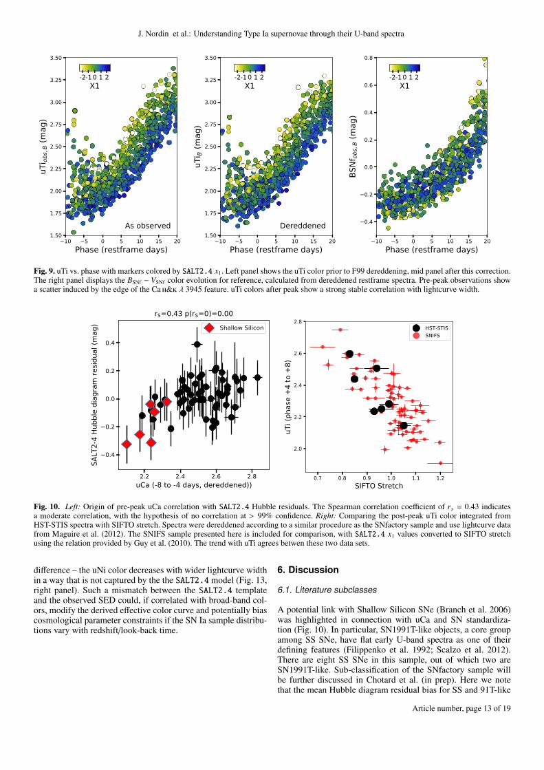
The Spearman rank correlation coefficient between SALT2.4Hubble residuals and pre-peak uCa is rs = 0.43, and the hypoth-esis of no correlation can be rejected at greater than 99% con-fidence (Fig. 10, left panel). We therefore test adding pre-peakuCa measurements as a further standardization parameter. Com-bining post-peak uTi and pre-peak uCa produces a Hubble dia-gram RMS of 0.086 ± 0.010 mag, while using only uCa and x1

reduced the RMS to 0.122±0.012 mag. The driving trend of thisimprovement can also be seen in Fig. 10: SNe Ia with large uCaindex are too bright after SALT2.4 standardization. Half of theseare classified as Branch Shallow Silicon objects – this connec-tion is further explored in Sec. 6.1.

We also note that the combined uTi + uCa fit producesa much reduced χ2 value, beyond what can be expected justthrough adding another fit parameter. When rerunning the stan-dardization without a fixed intrinsic dispersion we obtain χ2 =38.6 for 40 degrees of freedom, thus there is no need to addany additional dispersion to reach χ2/dof = 1. As the internalSALT2.4 model error propagates an effective intrinsic disper-sion of 0.055 mag, other fit methods are required to investigatewhether a fit without any added dispersion can be attained. Forcomparison, the uTi fit requires an intrinsic dispersion of σint =0.070 ± 0.009 mag and the x1 fit requires σint = 0.090 ± 0.008mag.

As a further test we evaluate the fit quality using the sample-size corrected Akaike Information Criteria (AICc), which penal-izes models with additional fit parameters. In Table 3 each linecompares uTi standardization (without any host galaxy propertycorrection) with one other combination of standardization prop-erty and host parameter. Each comparison includes all SNe avail-able for that combination of data, and shows both the differencein χ2 and the AICc probability ratio. Models including both uTiand uCa are strongly preferred over only using uTi, with a P-value of < 0.001, even though penalized for adding another fitparameter. Using only uTi is similarly favored compared withthe x1 fit.



3300 3500 4000 5000 6000

Wavelength (A)

1

2

3 SN2011fe @ peakSNF20080514-002 @ peak

Wavelength (A)

2

4

Flux

den

sity

(sca

led)

SNF20080514-002 @ peakFit to SNF080514-002Ti supressed


2

4 SN2011fe @ peakFit to SNF20080514-002Ti supressed

Fig. 7. Probing the origin of uTi variation through SYNAPPS model comparisons. The top panel compares SN2011fe and SNF20080514-002 atpeak light. The second panel shows SNF20080514-002 (orange line) together with the best SYNAPPS fit of this spectrum (black dashed line).The green line shows the same fit, but with the optical depth (τ) of Ti ii decreased by one dex, effectively suppressing these ions. The third panelcompares the SN2011fe spectrum with the same SNF20080514-002 SYNAPPS fits. The SNF200805014-002 fit with suppressed Ti ii optical depthmatches the SN2011fe λ(uTi) region well. Vertical dotted lines indicate the U-band spectral index boundaries, with λ(uTi) shaded light grey.

Table 2. Standardization fit results.

Fit parameters SNe χ2 χ2/dof HR RMS (mag) Host mass step (mag) LsSFR step (mag)

x1 73 70.76 1.00 0.135 ± 0.011 0.098 ± 0.031 −0.151 ± 0.028uTi@p6 57 44.18 0.80 0.116 ± 0.011 0.042 ± 0.031 −0.075 ± 0.031x1 (cut) 43 43.22 1.05 0.136 ± 0.015 0.094 ± 0.037 −0.156 ± 0.035uTi@p6 (cut) 43 27.21 0.66 0.105 ± 0.012 0.034 ± 0.033 −0.068 ± 0.034x1 + uCa@m6 52 40.90 0.83 0.122 ± 0.012 0.081 ± 0.033 −0.138 ± 0.030uTi@p6 + uCa@m6 43 18.22 0.46 0.086 ± 0.010 0.022 ± 0.030 −0.065 ± 0.030

Notes. The first column shows which standardization parameters are included (in addition to SALT2.4 color), where cut fits are restricted to SNewith measurements both at pre-peak and post-peak phases. The number of SNe included is given in the second column. The intrinsic dispersionwas fixed to 0.090 mag for all runs. The size of a step based on global host-galaxy mass or local age (LsSFR) were calculated as in R17 and areshown in the final two columns.

The significance of these improvements can also be numeri-cally investigated by re-fitting the standardization after randomlyredistributing the uCa measurements among SNe. When coupledto uTi, two out of 10000 random simulations yielded a similarlylow RMS, equivalent to a P-value of < 10−5. When combinedwith x1, zero out of 10000 did so.

Finally, the HST-STIS sample presented by Maguire et al.(2012) also included a small sample of spectra covering theλ(uTi) region and overlapping with the post-peak phase stud-ied here (phase +4 to +8 days). Lightcurve width information(“stretch” and B − V , determined by SIFTO) exists for sevenof these SNe (PTF10wof, PTF10ndc, PTF10qyx, PTF10qjl,PTF10yux, PTF09dnp, PTF10nlg). With these data we cancheck an external dataset for a similar correlation. We dered-

den the spectra as was done previously with the SNf data andcalculate the uTi color. Fig. 10 (right panel) shows a strong cor-relation for this small sample, compatible with the uTi trend dis-cussed above. We find that this trend agrees well with the SNIFSmeasurement presented here, after converting the latter to SIFTOstretch values.

5.2. The SN progenitor environment

The R17 analysis of the local host galaxy environment found thatSNe Ia in younger environments are 0.163 ± 0.029 mag (5.7σ)fainter than SNe Ia in older environments, after SALT2.4 stan-dardization (based on a larger sample than used here). The cor-responding analysis of global host galaxy mass found SNe Ia



Table 3. Each line shows Hubble residual fit quality for a given standardization method, measured relative to a reference fit based on post-peak uTidata without any host property corrections (first line). Each comparison is made using only the SNe in common (Nbr SNe) for a given measurement.The penultimate column shows the difference in χ2 assuming Hubble residuals are described using one or two Gaussian distributions (the latterwhen a host property step is included). The final column gives the likelihood according to the the sample-size corrected Akaike InformationCriteria (AICc), again relative to the first line uTi model.

Standardizing property Host step Nbr SNe χ2 − χ2uTi P(AICc) Ratio

uTi@p6 None 57 0 1.0Global mass 47 −1.9 0.19LsSFR 47 −4.8 0.84

x1 None 57 20.5 3.6e − 5Global mass 47 5.6 0.0045LsSFR 47 1.9 0.029

uTi@p6 + uCa@m6 None 43 −17.2 1521.5Global mass 35 −12.0 5.0LsSFR 35 −15.9 33.7


0.0

0.5

1.0

1.5

2.0

2.5

3.0

3.5

4.0

4.5

Flux

den

sity

(nor

mal

ized)

uNi

LSQ12fxd @ 8, x1 = 0.07 ± 0.13, n = 3.24+0.530.36

SN2011fe @ 8, x1 = 0.40 ± 0.11, n = 2.15 ± 0.02

Fig. 8. Spectra of SN2011fe and LSQ12fxd at phase ∼ −8 days.LSQ12fxd has, compared with SN2011fe, both a steeper early rise-time(Firth et al. 2015) and less flux in the λ(uNi) region (i.e. stronger Co iiabsorption at this phase).

in lower mass galaxies to be 0.119 ± 0.032 mag fainter thanthose in more massive hosts. We recover these trends for thesubset of SNe in this analysis with R17 measurements, finding a−0.151 ± 0.028 mag step for LsSFR and 0.098 ± 0.031 mag forglobal host galaxy mass.

When this step analysis is performed based on the standard-ization residuals where uTi replaced x1 the step sizes are reducedto 0.042±0.031 mag for mass and −0.075±0.031 mag for LsSFR(given in the final two columns of Table 2). uCa has less im-pact for environmental steps, producing modest step size reduc-tions to 0.022 ± 0.030 mag and −0.065 ± 0.030 mag. ∆χ2 andAICc probabilities for these models, again relative to applyinguTi but no host data, can also be found in Table 3. We find thatthe full model including uTi, uCa and LsSFR provides the small-est χ2/dof, but that the AICc find fits including uTi and uCa butno host corrections to be preferred considering the number ofparameters. The fit quality of the x1 models rapidly increases ashost information is included. Adding host information to the U-band parameter models is not justified as χ2 is only modestlyimproved.

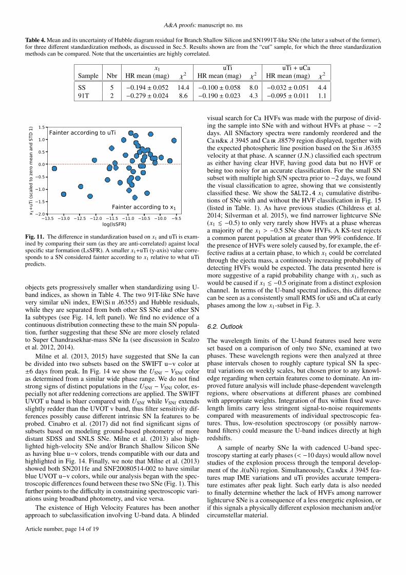
In Fig. 11 we search for the SNe for which lightcurve widthand uTi predict different magnitudes. As uTi and x1 are anti-

correlated, we can do this by normalizing both distributions tozero mean and unity RMS and then plotting the sum of the twotransformed values for each SN. Current x1 standardization pro-duces SN magnitudes that are too bright in passive environments(low LsSFR), i.e. the x1 parameter assumes these to be intrinsi-cally fainter than they actually are and overcorrects their magni-tudes. As is visualized in Fig. 11, uTi still predicts these SNeto be intrinsically faint, but not by as much as x1, thus gen-erating smaller magnitude corrections and avoiding overcorrec-tion. Similarly, in actively star forming regions uTi does not pre-dict SNe to be as intrinsically overluminous as predicted by x1.The variation in predicted peak magnitude as a function of hostgalaxy environment suggests an underlying property that varieswith age and affects the explosion duration (lightcurve width)without a corresponding change of the peak energy/temperaturewould cause a trend like the one observed. Further studies areneeded to investigate whether, for example, progenitor size couldact in this way.

The dependence on LsSFR can be visualized for this sam-ple by comparing peak magnitude (for clarity, after color cor-rection) versus SALT2.4 x1 (left panel of Fig. 12). For fixed x1,SNe in passive (“delayed”) environments are brighter. Perform-ing such a comparison for uTi shows the dependence on LsSFRto be much reduced (right panel of Fig. 12).

5.3. U-band indices and the choice of color curve

Here we first study the potential systematic error caused bydereddening using the F99 color curve, if in fact all SNe Ia ac-tually followed the SALT2.4 color curve. The systematic (theo-retical) change in the uNi, uTi, uSi and uCa color indices be-tween F99 and SALT2.4, as a function of the color parame-ter is shown in Fig. 13. We use the same conversion betweenE(B − V) and SALT2.4 c as previously. More than 90% of thesample has |c| < 0.15, a range where the maximum possible vari-ation for the uTi, uSi and uCa colors are limited to less than0.1 mag – small considering the U-band parameter value rangesfound here. We therefore conclude that the standardization ef-fects discussed above were not driven by systematic effects fromthe dereddening process.

An empirical SN Ia standardization model, like SALT2.4, re-lies on the combination of a color curve and a spectral model topredict how the intrinsic spectrum varies (for SALT the latter isparameterized by x1). Comparing the SALT2.4 spectral modelwith observations in the λ(uNi) region, where empirical and dustcolor curves start to strongly deviate, we note a clear functional



10 5 0 5 10 15 20Phase (restframe days)

1.50

1.75

2.00

2.25

2.50

2.75

3.00

3.25

3.50

uTi ob

s,B (m

ag)

As observed

-2-10 1 2X1


1.50

1.75

2.00

2.25

2.50

2.75

3.00

3.25

3.50

uTi B

(mag

)

Dereddened

-2-10 1 2X1


0.4

0.2

0.0

0.2

0.4

0.6

0.8

BSNf

obs,

B (m

ag)

-2-10 1 2X1

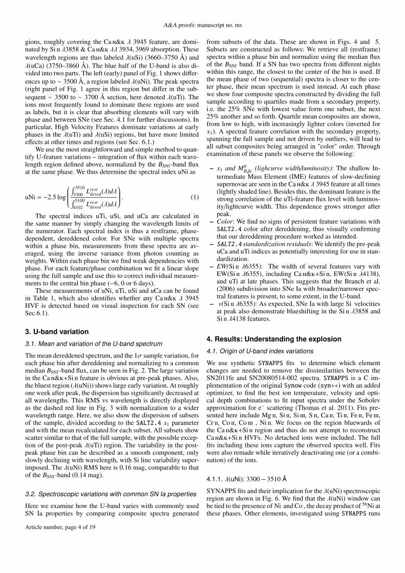
Fig. 9. uTi vs. phase with markers colored by SALT2.4 x1. Left panel shows the uTi color prior to F99 dereddening, mid panel after this correction.The right panel displays the BSNf − VSNf color evolution for reference, calculated from dereddened restframe spectra. Pre-peak observations showa scatter induced by the edge of the Ca h&k λ 3945 feature. uTi colors after peak show a strong stable correlation with lightcurve width.

2.2 2.4 2.6 2.8uCa (-8 to -4 days, dereddened))

0.4

0.2

0.0

0.2

0.4

SALT

2-4

Hubb

le d

iagr

am re

sidua

l (m

ag)

rS=0.43 p(rS=0)=0.00Shallow Silicon

0.7 0.8 0.9 1.0 1.1 1.2SIFTO Stretch

2.0

2.2

2.4

2.6

2.8

uTi (

phas

e +4

to +

8)

HST-STISSNIFS

Fig. 10. Left: Origin of pre-peak uCa correlation with SALT2.4 Hubble residuals. The Spearman correlation coefficient of rs = 0.43 indicatesa moderate correlation, with the hypothesis of no correlation at > 99% confidence. Right: Comparing the post-peak uTi color integrated fromHST-STIS spectra with SIFTO stretch. Spectra were dereddened according to a similar procedure as the SNfactory sample and use lightcurve datafrom Maguire et al. (2012). The SNIFS sample presented here is included for comparison, with SALT2.4 x1 values converted to SIFTO stretchusing the relation provided by Guy et al. (2010). The trend with uTi agrees betwen these two data sets.

difference – the uNi color decreases with wider lightcurve widthin a way that is not captured by the the SALT2.4 model (Fig. 13,right panel). Such a mismatch between the SALT2.4 templateand the observed SED could, if correlated with broad-band col-ors, modify the derived effective color curve and potentially biascosmological parameter constraints if the SN Ia sample distribu-tions vary with redshift/look-back time.

6. Discussion

6.1. Literature subclasses

A potential link with Shallow Silicon SNe (Branch et al. 2006)was highlighted in connection with uCa and SN standardiza-tion (Fig. 10). In particular, SN1991T-like objects, a core groupamong SS SNe, have flat early U-band spectra as one of theirdefining features (Filippenko et al. 1992; Scalzo et al. 2012).There are eight SS SNe in this sample, out of which two areSN1991T-like. Sub-classification of the SNfactory sample willbe further discussed in Chotard et al. (in prep). Here we notethat the mean Hubble diagram residual bias for SS and 91T-like



Table 4. Mean and its uncertainty of Hubble diagram residual for Branch Shallow Silicon and SN1991T-like SNe (the latter a subset of the former),for three different standardization methods, as discussed in Sec.5. Results shown are from the “cut” sample, for which the three standardizationmethods can be compared. Note that the uncertainties are highly correlated.

x1 uTi uTi + uCaSample Nbr HR mean (mag) χ2 HR mean (mag) χ2 HR mean (mag) χ2

SS 5 −0.194 ± 0.052 14.4 −0.100 ± 0.058 8.0 −0.032 ± 0.051 4.491T 2 −0.279 ± 0.024 8.6 −0.190 ± 0.023 4.3 −0.095 ± 0.011 1.1

13.5 13.0 12.5 12.0 11.5 11.0 10.5 10.0 9.5log(lsSFR)

2.0

1.5

1.0

0.5

0.0

0.5

1.0

1.5

x 1+u

Ti (s

cale

d to

zero

mea

n an

d ST

D 1)

Fainter according to x1

Fainter according to uTi

Fig. 11. The difference in standardization based on x1 and uTi is exam-ined by comparing their sum (as they are anti-correlated) against localspecific star formation (LsSFR). A smaller x1+uTi (y-axis) value corre-sponds to a SN considered fainter according to x1 relative to what uTipredicts.

objects gets progressively smaller when standardizing using U-band indices, as shown in Table 4. The two 91T-like SNe havevery similar uNi index, EW(Si ii λ6355) and Hubble residuals,while they are separated from both other SS SNe and other SNIa subtypes (see Fig. 14, left panel). We find no evidence of acontinuous distribution connecting these to the main SN popula-tion, further suggesting that these SNe are more closely relatedto Super Chandrasekhar-mass SNe Ia (see discussion in Scalzoet al. 2012, 2014).

Milne et al. (2013, 2015) have suggested that SNe Ia canbe divided into two subsets based on the SWIFT u−v color at±6 days from peak. In Fig. 14 we show the USNf − VSNf coloras determined from a similar wide phase range. We do not findstrong signs of distinct populations in the USNf − VSNf color, es-pecially not after reddening corrections are applied. The SWIFTUVOT u band is bluer compared with USNf while VSNf extendsslightly redder than the UVOT v band, thus filter sensitivity dif-ferences possibly cause different intrinsic SN Ia features to beprobed. Cinabro et al. (2017) did not find significant signs ofsubsets based on modeling ground-based photometry of moredistant SDSS and SNLS SNe. Milne et al. (2013) also high-lighted high-velocity SNe and/or Branch Shallow Silicon SNeas having blue u−v colors, trends compatible with our data andhighlighted in Fig. 14. Finally, we note that Milne et al. (2013)showed both SN2011fe and SNF20080514-002 to have similarblue UVOT u−v colors, while our analysis began with the spec-troscopic differences found between these two SNe (Fig. 1). Thisfurther points to the difficulty in constraining spectroscopic vari-ations using broadband photometry, and vice versa.

The existence of High Velocity Features has been anotherapproach to subclassification involving U-band data. A blinded

visual search for Ca HVFs was made with the purpose of divid-ing the sample into SNe with and without HVFs at phase ∼ −2days. All SNfactory spectra were randomly reordered and theCa h&k λ 3945 and Ca ir λ8579 region displayed, together withthe expected photospheric line position based on the Si ii λ6355velocity at that phase. A scanner (J.N.) classified each spectrumas either having clear HVF, having good data but no HVF orbeing too noisy for an accurate classification. For the small SNsubset with multiple high S/N spectra prior to −2 days, we foundthe visual classification to agree, showing that we consistentlyclassified these. We show the SALT2.4 x1 cumulative distribu-tions of SNe with and without the HVF classification in Fig. 15(listed in Table. 1). As have previous studies (Childress et al.2014; Silverman et al. 2015), we find narrower lightcurve SNe(x1 . −0.5) to only very rarely show HVFs at a phase whereasa majority of the x1 > −0.5 SNe show HVFs. A KS-test rejectsa common parent population at greater than 99% confidence. Ifthe presence of HVFs were solely caused by, for example, the ef-fective radius at a certain phase, to which x1 could be correlatedthrough the ejecta mass, a continously increasing probability ofdetecting HVFs would be expected. The data presented here ismore suggestive of a rapid probability change with x1, such aswould be caused if x1 . −0.5 originate from a distinct explosionchannel. In terms of the U-band spectral indices, this differencecan be seen as a consistently small RMS for uSi and uCa at earlyphases among the low x1-subset in Fig. 3.

6.2. Outlook

The wavelength limits of the U-band features used here wereset based on a comparison of only two SNe, examined at twophases. These wavelength regions were then analyzed at threephase intervals chosen to roughly capture typical SN Ia spec-tral variations on weekly scales, but chosen prior to any knowl-edge regarding when certain features come to dominate. An im-proved future analysis will include phase-dependent wavelengthregions, where observations at different phases are combinedwith appropriate weights. Integration of flux within fixed wave-length limits carry less stringent signal-to-noise requirementscompared with measurements of individual spectroscopic fea-tures. Thus, low-resolution spectroscopy (or possibly narrow-band filters) could measure the U-band indices directly at highredshifts.

A sample of nearby SNe Ia with cadenced U-band spec-troscopy starting at early phases (< −10 days) would allow novelstudies of the explosion process through the temporal develop-ment of the λ(uNi) region. Simultaneously, Ca h&k λ 3945 fea-tures map IME variations and uTi provides accurate tempera-ture estimates after peak light. Such early data is also neededto finally determine whether the lack of HVFs among narrowerlightcurve SNe is a consequence of a less energetic explosion, orif this signals a physically different explosion mechanism and/orcircumstellar material.



3 2 1 0 1 2x1 (SALT2.4)

0.4

0.2

0.0

0.2

0.4

Peak

mag

w. c

olor

cor

r. (M

Bc)

OlderYounger

1.9 2.0 2.1 2.2 2.3 2.4 2.5 2.6uTi (4 to 8 days, dereddened)

0.4

0.2

0.0

0.2

0.4

Peak

mag

w. c

olor

cor

r. (M

Bc)

OlderYounger

Fig. 12. Comparing peak SN magnitude (including color correction) with SALT2.4 x1 (left panel) and uTi (right panel). Lighter shaded pointswere found in R17 to originate in locally passive regions, and likely from old progenitors, while dark blue points were found in regions dominatedby star formation. These are separated in x1 (left), but not in uTi (right).

0.1 0.0 0.1 0.2 0.3SALT 2.4 c (Color)

0.4

0.3

0.2

0.1

0.0

0.1

0.2

U in

dex

chan

ge (S

ALT2

.4-f9

9)

uNiuTi

uSiuCa

2.4 2.6 2.8 3.0 3.2uNi (4 to 8 days, dereddened)

3

2

1

0

1

2

X 1

SALT2.4 prediction

Fig. 13. Left: Directly comparing the difference in U-band color indices, u(Ni|Ti|Si|Ca)SALT-u(Ni|Ti|Si|Ca)F99. While systematic differences growlarge for highly reddened objects, these are limited for the current sample. Orange, short, vertical lines show the SALT2.4 c values of SNe in thissample. Right: SALT x1 vs uNi at phase 4 to 8 days. The red line shows the corresponding SALT model predictions.

The limit at which HVFs disappear (x1 ∼ −0.5) agrees withwhere Scalzo et al. (2014), using SNfactory SNe with coverageextending to late phases, find that the derived ejecta mass (Me j)points to sub-Chandrasekhar mass explosions. The seven SNein the sample analyzed here with derived Me j and MNi massesfrom Scalzo et al. (2014) are insufficient for further tests of Me jand MNi correlations, again motivating larger samples whichcombine several types of observations. These could include alsoejecta/Ni /IGE constraints derived through nebular Co ii lines(Childress et al. 2015), second maximum position (Dhawan et al.2015) and early lightcurve rise-time (Firth et al. 2015), as wellas measurements of ejecta asymmetry from nebular lines (Maedaet al. 2011).

We see signs that the currently most widely used SN model,SALT2.4, can be improved. Updates to the SN template in thisregion could propagate into a change in the effective color law.Creating an unbiased template for the intrinsic U-band spec-trum is a requirement for current and future ground-based SNIa analyzes like DES and LSST, where the rest-frame U-band isredshifted to the wavelengths most efficiently observed from theground.

7. Summary and conclusions

Comparing spectra of two supernovae at early and peak phasesled to the subdivision of the U-band into four regions whose fluxratio relative to B-band were used to construct the uNi, uTi, uSiand uCa indices. We use a sample of 92 SNe Ia to analyze theseindices at three representative phase ranges: −8 to −4 days (pre-peak), −2 to 2 days (peak) and 4 to 8 days (post-peak). Based onthese measurements we find:

– SYNAPPS comparisons show that Ni/Co absorption can ex-plain differences in the bluest feature (“uNi”). uNi at pre-peak phases can be used as a probe of Ni abundance, to com-plement constraints from the early lightcurve rise-time, bolo-metric lightcurves and nebular emission.

– In similar tests, SYNAPPS fits also show that Ti absorptiondifferences dominate the λ(uTi) wavelength range. The uTiindex is an extremely sensitive luminosity indicator. Whenused instead of the SALT2.4 x1 parameter the RMS scatteraround the Hubble diagram falls to 0.116 ± 0.011 mag. Herewe use measurements made in the post-peak phase region,but note that the uTi index at all phases after peak is stronglycorrelated with lightcurve width.



20 40 60 80 100 120 140EW(SiII 6355) ( 2 to 2 days, Å)

1.4

1.6

1.8

2.0

2.2

uNi (

-8 to

-4 d

ays,

dere

dden

ed))

PTF10zdkShallow Silicon91T

0.2 0.1 0.0 0.1 0.2 0.3 0.4USNf VSNf (mag, phase 6 to 6 days)

0

2

4

6

8

10

12

14

16 No dereddeningw. dereddeningSS (dered)

Fig. 14. Left: uNi index measurements of SN1991T-like and Shallow Silicon-like SNe Ia compared with EW(Si ii λ6355). The SN1991T-like SNeare disconnected from the remaining sample. Right: Distribution of USNf −VSNf for spectra within 6 days of lightcurve peak. The figure shows datawith (orange) and without (blue) reddening correction, where the linear evolution with phase was removed for each (returning distributions withzero mean). The Shallow Silicon (SS) subset of the dereddened USNf − VSNf distribution is shown by the cross-hatched histogram.

2 1 0 1 2SALT x1

0.0

0.2

0.4

0.6

0.8

1.0

Cum

ulat

ive

dist

ribut

ion High velocity CaH&K

No visual high velocity

Fig. 15. Cumulative x1 distributions for SNe with and without visuallyidentified High Velocity Features (based on spectra with phase < −2day).

– Adding pre-peak uCa as a third standardization parameterfurther reduces the RMS around the Hubble diagram. A fitwith uTi and uCa yields a 0.086 ± 0.010 mag scatter withχ2/dof ∼ 1 without the need to introduce intrinsic disper-sion.

– Including U-band indices in SN Ia standardization reducesthe dependence on host-galaxy environment. The differencebetween lightcurve width and uTi can be used to study SN Iaprogenitor scenarios.

– Shallow Silicon and 91T-like SNe have biased SALT2.4Hubble residuals, which are substantially reduced when U-band parameters are included in the fit. The two 91T-like SNein this sample have similar U-band properties and magni-tudes, which are offset from the remaining sample.

– We confirm previous results that narrower-lightcurve SNe Iavery rarely show HVFs. We find a sharp transition in theirincidence at x1 = −0.5.

Acknowledgements. We thank the technical staff of the University of Hawaii 2.2m telescope, and Dan Birchall for observing assistance. We recognize the signif-icant cultural role of Mauna Kea within the indigenous Hawaiian community,and we appreciate the opportunity to conduct observations from this reveredsite. This work was supported in part by the Director, Office of Science, Of-fice of High Energy Physics of the U.S. Department of Energy under ContractNo. DE-AC02-05CH11231. Support in France was provided by CNRS/IN2P3,CNRS/INSU, and PNC; LPNHE acknowledges support from LABEX ILP, sup-ported by French state funds managed by the ANR within the Investissementsd’Avenir programme under reference ANR-11-IDEX-0004-02. Support in Ger-many was provided by DFG through TRR33 “The Dark Universe” and by DLRthrough grants FKZ 50OR1503 and FKZ 50OR1602. In China the support wasprovided from Tsinghua University 985 grant and NSFC grant No 11173017.Some results were obtained using resources and support from the National En-ergy Research Scientific Computing Center, supported by the Director, Office ofScience, Office of Advanced Scientific Computing Research of the U.S. Depart-ment of Energy under Contract No. DE-AC02- 05CH11231. We thank the Gor-don & Betty Moore Foundation for their continuing support. Additional supportwas provided by NASA under the Astrophysics Data Analysis Program grant15-ADAP15-0256 (PI: Aldering). We also thank the High Performance Researchand Education Network (HPWREN), supported by National Science FoundationGrant Nos. 0087344 & 0426879.

ReferencesAldering, G., Adam, G., Antilogus, P., et al. 2002, Proc. SPIE, 4836, 61Aldering, G., Antilogus, P., Bailey, S., et al. 2006, ApJ, 650, 510Altavilla, G., Stehle, M., Ruiz-Lapuente, P., et al. 2007, A&A, 475, 585Amanullah, R., Johansson, J., Goobar, A., et al. 2015, MNRAS, 453, 3300Arsenijevic, V., Fabbro, S., Mourão, A. M., & Rica da Silva, A. J. 2008, A&A,

492, 535Bacon, R., Copin, Y., Monnet, G., et al. 2001, MNRAS, 326, 23Betoule, M., Kessler, R., Guy, J., et al. 2014, A&A, 568, A22Blondin, S., Dessart, L., Hillier, D. J., & Khokhlov, A. M. 2013, MNRAS, 429,

2127Blondin, S., Matheson, T., Kirshner, R. P., et al. 2012, AJ, 143, 126Bloom, J. S., Kasen, D., Shen, K. J., et al. 2012, ApJ, 744, L17Bongard, S., Soulez, F., Thiébaut, É., & Pecontal, É. 2011, MNRAS, 418, 258Branch, D., Dang, L. C., Hall, N., et al. 2006, PASP, 118, 560Bufano, F., Immler, S., Turatto, M., et al. 2009, ApJ, 700, 1456Burns, C. R., Stritzinger, M., Phillips, M. M., et al. 2014, ApJ, 789, 32



Buton, C., Copin, Y., Aldering, G., et al. 2013, A&A, 549, A8Cao, Y., Johansson, J., Nugent, P. E., et al. 2016, ApJ, 823, 147Cartier, R., Sullivan, M., Firth, R. E., et al. 2017, MNRAS, 464, 4476Childress, M., Aldering, G., Antilogus, P., et al. 2013a, ApJ, 770, 108Childress, M., Aldering, G., Antilogus, P., et al. 2013b, ApJ, 770, 107Childress, M. J., Filippenko, A. V., Ganeshalingam, M., & Schmidt, B. P. 2014,

MNRAS, 437, 338Childress, M. J., Hillier, D. J., Seitenzahl, I., et al. 2015, MNRAS, 454, 3816Chornock, R., Berger, E., Rest, A., et al. 2013, ApJ, 767, 162Chotard, N. 2011, Theses, Université Claude Bernard - Lyon IChotard, N., Gangler, E., Aldering, G., et al. 2011, A&A, 529, L4Cinabro, D., Scolnic, D., Kessler, R., Li, A., & Miller, J. 2017, MNRAS, 466,

884Dhawan, S., Leibundgut, B., Spyromilio, J., & Maguire, K. 2015, MNRAS, 448,

1345Dilday, B., Howell, D. A., Cenko, S. B., et al. 2012, Science, 337, 942Edwards, Z. I., Pagnotta, A., & Schaefer, B. E. 2012, ApJ, 747, L19Ellis, R. S., Sullivan, M., Nugent, P. E., et al. 2008, ApJ, 674, 51Fakhouri, H. K., Boone, K., Aldering, G., et al. 2015, ApJ, 815, 58Feindt, U., Kerschhaggl, M., Kowalski, M., et al. 2015, A&A, 578, C1Filippenko, A. V., Richmond, M. W., Matheson, T., et al. 1992, ApJ, 384, L15Firth, R. E., Sullivan, M., Gal-Yam, A., et al. 2015, MNRAS, 446, 3895Fitzpatrick, E. L. 1999, PASP, 111, 63Foley, R. J. 2013, MNRAS, 435, 273Foley, R. J., Filippenko, A. V., Kessler, R., et al. 2012, AJ, 143, 113Foley, R. J., Pan, Y.-C., Brown, P., et al. 2016, MNRAS, 461, 1308Foley, R. J., Sanders, N. E., & Kirshner, R. P. 2011, ApJ, 742, 89Garavini, G., Folatelli, G., Goobar, A., et al. 2004, AJ, 128, 387Garavini, G., Nobili, S., Taubenberger, S., et al. 2007, A&A, 471, 527Guy, J., Sullivan, M., Conley, A., et al. 2010, A&A, 523, A7Hachinger, S., Mazzali, P. A., Sullivan, M., et al. 2013, MNRAS, 429, 2228Hamuy, M., Phillips, M. M., Suntzeff, N. B., et al. 2003, Nature, 424, 651Hayden, B. T., Garnavich, P. M., Kasen, D., et al. 2010, ApJ, 722, 1691Huang, X., Raha, Z., Aldering, G., et al. 2017, ApJ, 836, 157Kessler, R., Becker, A. C., Cinabro, D., et al. 2009, ApJS, 185, 32Kromer, M., Sim, S. A., Fink, M., et al. 2010, ApJ, 719, 1067Lantz, B., Aldering, G., Antilogus, P., et al. 2004, in Proc. SPIE, Vol. 5249, Op-

tical Design and Engineering, ed. L. Mazuray, P. J. Rogers, & R. Wartmann,146–155

Leonard, D. C. 2007, ApJ, 670, 1275Li, W., Bloom, J. S., Podsiadlowski, P., et al. 2011, Nature, 480, 348Maeda, K., Leloudas, G., Taubenberger, S., et al. 2011, MNRAS, 413, 3075Maeda, K. & Terada, Y. 2016, International Journal of Modern Physics D, 25,

1630024Maguire, K., Sullivan, M., Ellis, R. S., et al. 2012, MNRAS, 426, 2359Maguire, K., Taubenberger, S., Sullivan, M., & Mazzali, P. A. 2016, MNRAS,

457, 3254Mandel, K. S., Scolnic, D. M., Shariff, H., Foley, R. J., & Kirshner, R. P. 2017,

ApJ, 842, 93Maoz, D., Mannucci, F., & Nelemans, G. 2014, ARA&A, 52, 107Matheson, T., Kirshner, R. P., Challis, P., et al. 2008, AJ, 135, 1598Mazzali, P. A., Benetti, S., Altavilla, G., et al. 2005, ApJ, 623, L37Miles, B. J., van Rossum, D. R., Townsley, D. M., et al. 2016, ApJ, 824, 59Milne, P. A., Brown, P. J., Roming, P. W. A., Bufano, F., & Gehrels, N. 2013,

ApJ, 779, 23Milne, P. A., Foley, R. J., Brown, P. J., & Narayan, G. 2015, ApJ, 803, 20Nordin, J., Östman, L., Goobar, A., et al. 2011, A&A, 526, A119Nugent, P., Phillips, M., Baron, E., Branch, D., & Hauschildt, P. 1995, ApJ, 455,

L147Pakmor, R., Kromer, M., Taubenberger, S., et al. 2012, ApJ, 747, L10Patat, F., Benetti, S., Cappellaro, E., et al. 1996, MNRAS, 278, 111Perlmutter, S., Aldering, G., Goldhaber, G., et al. 1999, ApJ, 517, 565Pinto, P. A. & Eastman, R. G. 2000, ApJ, 530, 757Piro, A. L. & Morozova, V. S. 2016, ApJ, 826, 96Piro, A. L. & Nakar, E. 2014, ApJ, 784, 85Quimby, R. M., Oguri, M., More, A., et al. 2014, Science, 344, 396Quimby, R. M., Werner, M. C., Oguri, M., et al. 2013, ApJ, 768, L20Riess, A. G., Filippenko, A. V., Challis, P., et al. 1998, AJ, 116, 1009Rigault, M., Aldering, G., Kowalski, M., et al. submitted, A&A, (R17)Rigault, M., Copin, Y., Aldering, G., et al. 2013, A&A, 560, A66, (R13)Röpke, F. K., Kromer, M., Seitenzahl, I. R., et al. 2012, ApJ, 750, L19Rubin, D., Aldering, G., Barbary, K., et al. 2015, ApJ, 813, 137Ruiter, A. J., Belczynski, K., Sim, S. A., et al. 2011, MNRAS, 417, 408Saunders, C., Aldering, G., Antilogus, P., et al. 2015, ApJ, 800, 57Scalzo, R., Aldering, G., Antilogus, P., et al. 2012, ApJ, 757, 12Scalzo, R., Aldering, G., Antilogus, P., et al. 2014, MNRAS, 440, 1498Scalzo, R. A., Aldering, G., Antilogus, P., et al. 2010, ApJ, 713, 1073Schaefer, B. E. & Pagnotta, A. 2012, Nature, 481, 164Schlegel, D. J., Finkbeiner, D. P., & Davis, M. 1998, ApJ, 500, 525Scolnic, D. M., Riess, A. G., Foley, R. J., et al. 2014, ApJ, 780, 37Seitenzahl, I. R., Ciaraldi-Schoolmann, F., Röpke, F. K., et al. 2014, MNRAS,

444, 350Silverman, J. M., Foley, R. J., Filippenko, A. V., et al. 2012, MNRAS, 425, 1789Silverman, J. M., Vinkó, J., Marion, G. H., et al. 2015, MNRAS, 451, 1973Sim, S. A., Röpke, F. K., Hillebrandt, W., et al. 2010, ApJ, 714, L52Sim, S. A., Seitenzahl, I. R., Kromer, M., et al. 2013, MNRAS, 436, 333Smitka, M. T., Brown, P. J., Suntzeff, N. B., et al. 2015, ApJ, 813, 30Stanishev, V., Goobar, A., Benetti, S., et al. 2007, A&A, 469, 645Sullivan, M., Conley, A., Howell, D. A., et al. 2010, MNRAS, 406, 782Tanaka, M., Mazzali, P. A., Benetti, S., et al. 2008, ApJ, 677, 448Tanaka, M., Mazzali, P. A., Maeda, K., & Nomoto, K. 2006, ApJ, 645, 470Thomas, R. C., Nugent, P. E., & Meza, J. C. 2011, PASP, 123, 237Timmes, F. X., Brown, E. F., & Truran, J. W. 2003, ApJ, 590, L83Walker, E. S., Hachinger, S., Mazzali, P. A., et al. 2012, MNRAS, 427, 103Wang, X., Li, W., Filippenko, A. V., et al. 2009, ApJ, 697, 380Wang, X., Wang, L., Filippenko, A. V., et al. 2012, ApJ, 749, 126



Appendix A: Element contributions to SYNAPPSfits.

We discuss in Sec. 4.1 how the observed spectral differencesbetween SN2011fe and SNF20080514-002 can be explainedby changing the early Ni/Co abundance and Ti abundance atpeak. Here we show the complete set of ion contributions to thebest fit SYNAPPS spectrum of SN2011fe 10 days prior to peak(Fig. A.1) and for SN200805014-002 close to peak (Fig. A.2).These fits match the observed data well.



3500 4000 4500 5000 5500 6000 6500Wavelength (Å)

12

10

8

6

4

2

0

2

4

F

lux

dens

ity ra

tio +

con

st.

R

elat

ive

flux

dens

ity

CoIIMgIISiIISIICaIIFeIIFeIIICoIIINiIICrIITiIISiIII

uNi uTi uSiuCa Full fit Observed spectrum

Fig. A.1. SYNAPPS fit to SN2011fe 10 days prior to peak. The top panel compares the observed spectrum to the full SYNAPPS fit. The lowerpanels show the contribution of each ion to the final spectra. These are plotted as the ratio between the spectrum with and without each ionactivated. Dashed, vertical, grey lines indicate the U-band index region boundaries, with designations given at the top.

3500 4000 4500 5000 5500 6000 6500Wavelength (Å)

12

10

8

6

4

2

0

2

4

F

lux

dens

ity ra

tio +

con

st.

R

elat

ive

flux

dens

ity

FeIIIMgIISiIISIICaIIFeIICoIIICoIINiIICrIITiIISiIII

uNi uTi uSiuCa Full fit Observed spectrum

Fig. A.2. SYNAPPS fit to SNF20080514-002 at peak light. The top panel compares the observed spectrum to the full SYNAPPS fit. The lowerpanels show the contribution of each ion to the final spectra. These are plotted as the ratio between the spectrum with and without each ionactivated. Dashed, vertical, grey lines indicate the U-band index region boundaries, with designations given at the top.


understanding type ia supernovae through their u ... - arxiv · 2 physics division, lawrence...

Documents