IOP PUBLISHING BIOINSPIRATION & BIOMIMETICS

Bioinspir. Biomim. 8 (2013) 046013 (15pp) doi:10.1088/1748-3182/8/4/046013

Understanding undulatory locomotion infishes using an inertia-compensatedflapping foil robotic deviceLi Wen1,2 and George Lauder1

1 The Museum of Comparative Zoology, 26 Oxford St., Harvard University, Cambridge, MA 02138, USA2 School of Mechanical Engineering and Automation, Beihang University, Beijing, 100191,People’s Republic of China

E-mail: liwen@buaa.edu.cn and glauder@oeb.harvard.edu

Received 21 August 2013Accepted for publication 7 November 2013Published 21 November 2013Online at stacks.iop.org/BB/8/046013

AbstractRecent advances in understanding fish locomotion with robotic devices have included the useof flapping foil robots that swim at a constant swimming speed. However, the speed of evensteadily swimming live fishes is not constant because the fish center of mass oscillates axiallythroughout a tail beat cycle. In this paper, we couple a linear motor that produces controlledoscillations in the axial direction to a robotic flapping foil apparatus to model both axial andside to side oscillatory motions used by freely-swimming fishes. This experimentalarrangement allows us to compensate for the substantial inertia of the carriage and motors thatdrive the oscillating foils. We identify a ‘critically-oscillated’ amplitude of axial motion atwhich the cyclic oscillations in axial locomotor force are greatly reduced throughout theflapping cycle. We studied the midline kinematics, power consumption and wake flow patternsof non-rigid foils with different lengths and flexural stiffnesses at a variety of axial oscillationamplitudes. We found that ‘critically-oscillated’ peak-to-peak axial amplitudes on the order of1.0 mm and at the correct phase are sufficient to mimic center of mass motion, and that suchamplitudes are similar to center of mass oscillations recorded for freely-swimming live fishes.Flow visualization revealed differences in wake flows of flexible foils between the‘non-oscillated’ and ‘critically-oscillated’ states. Inertia-compensating methods provide anovel experimental approach for studying aquatic animal swimming, and allow instrumentedrobotic swimmers to display center of mass oscillations similar to those exhibited byfreely-swimming fishes.

(Some figures may appear in colour only in the online journal)

1. Introduction

Recent advances in understanding undulatory fish locomotion,in which wave-like motions of the body generate propulsiveforces, have included the use of robotic flapping foil deviceswhich exhibit a rich variety of dynamic behaviors similarto the undulatory motions of live swimming fish (e.g.,Triantafyllou et al 2000, Lauder 2011). The analysis offlapping models swimming under controlled conditions hasattracted mathematicians (Alben et al 2012), fluid engineers(Anderson et al 1998, Buchholz and Smits 2008, Read et al

2003, Techet 2008), roboticists (Barrett et al 1999, Wen et al2012, Low and Chong 2010) and biologists (Blevins andLauder 2013, Fish et al 2006, Lauder and Madden 2006)interested in studying the principles underlying unsteadylocomotion in aquatic animals. Recent work has includedthe study of passive flexible swimming foils which producemovements generally similar to swimming fishes to mimicundulatory body motion (Lauder et al 2007, 2011a, 2011b,Oeffner and Lauder 2012).

These recent studies tend to emphasize the locomotionof freely-moving foil models under self-propelled conditions.

1748-3182/13/046013+15$33.00 1 © 2013 IOP Publishing Ltd Printed in the UK & the USA

Bioinspir. Biomim. 8 (2013) 046013 L Wen and G Lauder

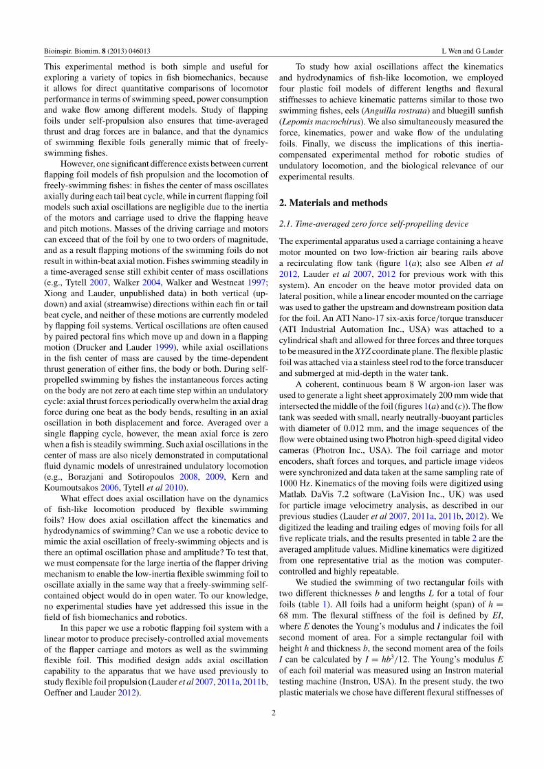
This experimental method is both simple and useful forexploring a variety of topics in fish biomechanics, becauseit allows for direct quantitative comparisons of locomotorperformance in terms of swimming speed, power consumptionand wake flow among different models. Study of flappingfoils under self-propulsion also ensures that time-averagedthrust and drag forces are in balance, and that the dynamicsof swimming flexible foils generally mimic that of freely-swimming fishes.

However, one significant difference exists between currentflapping foil models of fish propulsion and the locomotion offreely-swimming fishes: in fishes the center of mass oscillatesaxially during each tail beat cycle, while in current flapping foilmodels such axial oscillations are negligible due to the inertiaof the motors and carriage used to drive the flapping heaveand pitch motions. Masses of the driving carriage and motorscan exceed that of the foil by one to two orders of magnitude,and as a result flapping motions of the swimming foils do notresult in within-beat axial motion. Fishes swimming steadily ina time-averaged sense still exhibit center of mass oscillations(e.g., Tytell 2007, Walker 2004, Walker and Westneat 1997;Xiong and Lauder, unpublished data) in both vertical (up-down) and axial (streamwise) directions within each fin or tailbeat cycle, and neither of these motions are currently modeledby flapping foil systems. Vertical oscillations are often causedby paired pectoral fins which move up and down in a flappingmotion (Drucker and Lauder 1999), while axial oscillationsin the fish center of mass are caused by the time-dependentthrust generation of either fins, the body or both. During self-propelled swimming by fishes the instantaneous forces actingon the body are not zero at each time step within an undulatorycycle: axial thrust forces periodically overwhelm the axial dragforce during one beat as the body bends, resulting in an axialoscillation in both displacement and force. Averaged over asingle flapping cycle, however, the mean axial force is zerowhen a fish is steadily swimming. Such axial oscillations in thecenter of mass are also nicely demonstrated in computationalfluid dynamic models of unrestrained undulatory locomotion(e.g., Borazjani and Sotiropoulos 2008, 2009, Kern andKoumoutsakos 2006, Tytell et al 2010).

What effect does axial oscillation have on the dynamicsof fish-like locomotion produced by flexible swimmingfoils? How does axial oscillation affect the kinematics andhydrodynamics of swimming? Can we use a robotic device tomimic the axial oscillation of freely-swimming objects and isthere an optimal oscillation phase and amplitude? To test that,we must compensate for the large inertia of the flapper drivingmechanism to enable the low-inertia flexible swimming foil tooscillate axially in the same way that a freely-swimming self-contained object would do in open water. To our knowledge,no experimental studies have yet addressed this issue in thefield of fish biomechanics and robotics.

In this paper we use a robotic flapping foil system with alinear motor to produce precisely-controlled axial movementsof the flapper carriage and motors as well as the swimmingflexible foil. This modified design adds axial oscillationcapability to the apparatus that we have used previously tostudy flexible foil propulsion (Lauder et al 2007, 2011a, 2011b,Oeffner and Lauder 2012).

To study how axial oscillations affect the kinematicsand hydrodynamics of fish-like locomotion, we employedfour plastic foil models of different lengths and flexuralstiffnesses to achieve kinematic patterns similar to those twoswimming fishes, eels (Anguilla rostrata) and bluegill sunfish(Lepomis macrochirus). We also simultaneously measured theforce, kinematics, power and wake flow of the undulatingfoils. Finally, we discuss the implications of this inertia-compensated experimental method for robotic studies ofundulatory locomotion, and the biological relevance of ourexperimental results.

2. Materials and methods

2.1. Time-averaged zero force self-propelling device

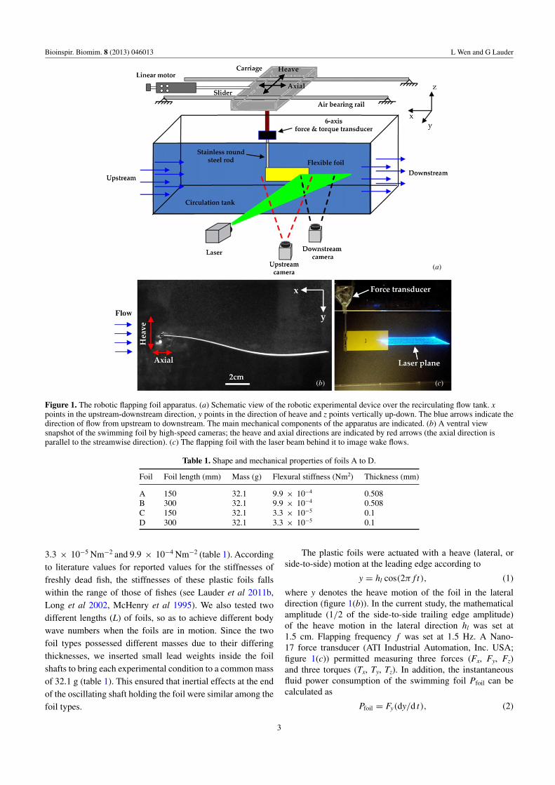
The experimental apparatus used a carriage containing a heavemotor mounted on two low-friction air bearing rails abovea recirculating flow tank (figure 1(a); also see Alben et al2012, Lauder et al 2007, 2012 for previous work with thissystem). An encoder on the heave motor provided data onlateral position, while a linear encoder mounted on the carriagewas used to gather the upstream and downstream position datafor the foil. An ATI Nano-17 six-axis force/torque transducer(ATI Industrial Automation Inc., USA) was attached to acylindrical shaft and allowed for three forces and three torquesto be measured in the XYZ coordinate plane. The flexible plasticfoil was attached via a stainless steel rod to the force transducerand submerged at mid-depth in the water tank.

A coherent, continuous beam 8 W argon-ion laser wasused to generate a light sheet approximately 200 mm wide thatintersected the middle of the foil (figures 1(a) and (c)). The flowtank was seeded with small, nearly neutrally-buoyant particleswith diameter of 0.012 mm, and the image sequences of theflow were obtained using two Photron high-speed digital videocameras (Photron Inc., USA). The foil carriage and motorencoders, shaft forces and torques, and particle image videoswere synchronized and data taken at the same sampling rate of1000 Hz. Kinematics of the moving foils were digitized usingMatlab. DaVis 7.2 software (LaVision Inc., UK) was usedfor particle image velocimetry analysis, as described in ourprevious studies (Lauder et al 2007, 2011a, 2011b, 2012). Wedigitized the leading and trailing edges of moving foils for allfive replicate trials, and the results presented in table 2 are theaveraged amplitude values. Midline kinematics were digitizedfrom one representative trial as the motion was computer-controlled and highly repeatable.

We studied the swimming of two rectangular foils withtwo different thicknesses b and lengths L for a total of fourfoils (table 1). All foils had a uniform height (span) of h =68 mm. The flexural stiffness of the foil is defined by EI,where E denotes the Young’s modulus and I indicates the foilsecond moment of area. For a simple rectangular foil withheight h and thickness b, the second moment area of the foilsI can be calculated by I = hb3/12. The Young’s modulus Eof each foil material was measured using an Instron materialtesting machine (Instron, USA). In the present study, the twoplastic materials we chose have different flexural stiffnesses of

2

Bioinspir. Biomim. 8 (2013) 046013 L Wen and G Lauder

(a)

(c)(b)

Figure 1. The robotic flapping foil apparatus. (a) Schematic view of the robotic experimental device over the recirculating flow tank. xpoints in the upstream-downstream direction, y points in the direction of heave and z points vertically up-down. The blue arrows indicate thedirection of flow from upstream to downstream. The main mechanical components of the apparatus are indicated. (b) A ventral viewsnapshot of the swimming foil by high-speed cameras; the heave and axial directions are indicated by red arrows (the axial direction isparallel to the streamwise direction). (c) The flapping foil with the laser beam behind it to image wake flows.

Table 1. Shape and mechanical properties of foils A to D.

Foil Foil length (mm) Mass (g) Flexural stiffness (Nm2) Thickness (mm)

A 150 32.1 9.9 × 10−4 0.508B 300 32.1 9.9 × 10−4 0.508C 150 32.1 3.3 × 10−5 0.1D 300 32.1 3.3 × 10−5 0.1

3.3 × 10−5 Nm−2 and 9.9 × 10−4 Nm−2 (table 1). Accordingto literature values for reported values for the stiffnesses offreshly dead fish, the stiffnesses of these plastic foils fallswithin the range of those of fishes (see Lauder et al 2011b,Long et al 2002, McHenry et al 1995). We also tested twodifferent lengths (L) of foils, so as to achieve different bodywave numbers when the foils are in motion. Since the twofoil types possessed different masses due to their differingthicknesses, we inserted small lead weights inside the foilshafts to bring each experimental condition to a common massof 32.1 g (table 1). This ensured that inertial effects at the endof the oscillating shaft holding the foil were similar among thefoil types.

The plastic foils were actuated with a heave (lateral, orside-to-side) motion at the leading edge according to

y = hl cos(2π f t), (1)

where y denotes the heave motion of the foil in the lateraldirection (figure 1(b)). In the current study, the mathematicalamplitude (1/2 of the side-to-side trailing edge amplitude)of the heave motion in the lateral direction hl was set at1.5 cm. Flapping frequency f was set at 1.5 Hz. A Nano-17 force transducer (ATI Industrial Automation, Inc. USA;figure 1(c)) permitted measuring three forces (Fx, Fy, Fz)and three torques (Tx, Ty, Tz). In addition, the instantaneousfluid power consumption of the swimming foil Pfoil can becalculated as

Pfoil = Fy(dy/d t), (2)

3

Bioinspir. Biomim. 8 (2013) 046013 L Wen and G Lauder

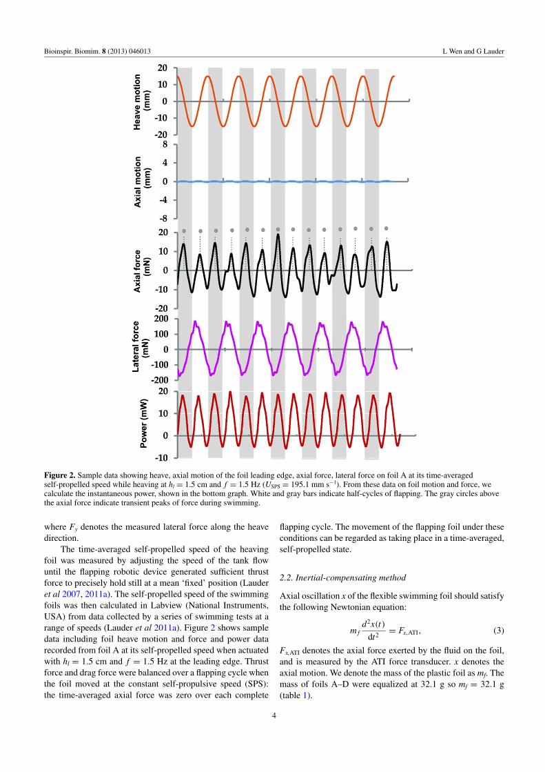
Figure 2. Sample data showing heave, axial motion of the foil leading edge, axial force, lateral force on foil A at its time-averagedself-propelled speed while heaving at hl = 1.5 cm and f = 1.5 Hz (USPS = 195.1 mm s−1). From these data on foil motion and force, wecalculate the instantaneous power, shown in the bottom graph. White and gray bars indicate half-cycles of flapping. The gray circles abovethe axial force indicate transient peaks of force during swimming.

where Fy denotes the measured lateral force along the heavedirection.

The time-averaged self-propelled speed of the heavingfoil was measured by adjusting the speed of the tank flowuntil the flapping robotic device generated sufficient thrustforce to precisely hold still at a mean ‘fixed’ position (Lauderet al 2007, 2011a). The self-propelled speed of the swimmingfoils was then calculated in Labview (National Instruments,USA) from data collected by a series of swimming tests at arange of speeds (Lauder et al 2011a). Figure 2 shows sampledata including foil heave motion and force and power datarecorded from foil A at its self-propelled speed when actuatedwith hl = 1.5 cm and f = 1.5 Hz at the leading edge. Thrustforce and drag force were balanced over a flapping cycle whenthe foil moved at the constant self-propulsive speed (SPS):the time-averaged axial force was zero over each complete

flapping cycle. The movement of the flapping foil under theseconditions can be regarded as taking place in a time-averaged,self-propelled state.

2.2. Inertial-compensating method

Axial oscillation x of the flexible swimming foil should satisfythe following Newtonian equation:

m fd2x(t)

dt2= Fx,ATI, (3)

Fx,ATI denotes the axial force exerted by the fluid on the foil,and is measured by the ATI force transducer. x denotes theaxial motion. We denote the mass of the plastic foil as mf. Themass of foils A–D were equalized at 32.1 g so mf = 32.1 g(table 1).

4

Bioinspir. Biomim. 8 (2013) 046013 L Wen and G Lauder

(b)

(a)

Figure 3. (a) The time history of axial and heave motions; ϕ indicates the phase between heave and axial movement. (b) Leading edgetrajectories of the foil at different phases ϕ. For panel (b), both the x- and y-axis scales are in mm.

Without the addition of an inertial-compensating linearmotor (discussed below), we measured the amplitude ofaxial carriage oscillation at approximately 0.05 mm whenthe foils were self-propelling. Why is the axial oscillationonly 0.05 mm? With the whole carriage set on low-frictionair bearings, the dynamics of the swimming foil satisfy thefollowing:

(Mc + m f )d2x(t)

d t2= Fx,AT I . (4)

The components on the carriage include motors, airbearings and other parts of the mechanical drive system(Lauder et al 2007), which have a total mass of Mc. The carriagemass Mc is approximately 8 kg, which is much more massivethan the plastic foil of 32.1 g: i.e. Mc � Mf. At self-propulsion,the axial forces produced by the swimming plastic foils are onthe order of only 10 mN (figure 2), and such a small forcecannot oscillate the heavy carriage axially to any significantextent.

To examine the effect of axial oscillations on swimmingfoils we used a linear motor system to provide appropriateaxial motion to actively compensate for the inertia of thecarriage and driving motors. We used a linear motor P01–23 × 160 controlled by E1100Gp (Linmot Inc., USA), with amovement repeatability of 0.05 mm, which allowed the axialmotion to be accurately controlled. We then mounted the linear

motor on the edge of the flow tank, and used a magneticlinear motor slider PL01-12 × 270/170 (Linmot Inc., USA)to push and pull the whole carriage set on the low-frictionair bearing rails (figure 1(a)). A synchronizing trigger fromthe Labview control program allowed us to control the phaseof linear motor axial oscillation with respect to foil heavemotion, and synchronized axial foil motion, force and torquedata acquisition, and image acquisition with two high-speedcameras for flow visualization.

The axial motion of the linear motor was programmed asfollows:

x = ha sin(4π f t + ϕ), (5)

where ha indicates the amplitude of the axial oscillation, and ϕ

is the phase difference between the axial and heave motions. Asshown in figure 3(a), the axial motion was programmed to havetwice the frequency of the heave oscillation. This is because theaxial force in swimming foils oscillates at twice the frequencyof the heave motion (see figure 2 for notation). Two axialforce peaks during one flapping cycle have also been observedin previous studies of the unsteady cyclic motion of bothswimming and flying animals (Triantafyllou et al 2005, Lauderet al 2011a, Sun and Wu 2003) and in computational analysesof fish undulatory propulsion (Borazjani and Sotiropoulos2008, 2009). We also measured the mechanical time lag and

5

Bioinspir. Biomim. 8 (2013) 046013 L Wen and G Lauder

delay in stroke reversal of the linear motor slider includingthe mechanical connection to the carriage to be approximately0.04 s. This backlash was then compensated for during dataprocessing to obtain an accurate phase ϕ.

We used two methods to quantify how the axial motionaffects fluctuations in the measured instantaneous axial force:root-mean-square (RMS), and average cyclic height (ACH).RMS for the instantaneous force measured over five cyclescan be defined as:

RMS =√

1

5T

∫ 5T

0( f (t))2d t. (6)

In the current study, the ACH was also used to describe theaverage peak-to-peak axial force between the cyclic maximaand minima during five flapping cycles. Measurements of RMSand ACH were done using Labchart 7 (ADI Instruments Inc.,USA).

In order to quantify how much inertial force was producedby the foil alone, we measured the inertial force generated inair by the axial motion in the absence of the heave motionwith different linear motor programs. For these inertial forcetests, we used a ‘weight model’ made of lead wire, with amass equal to that of the foils (32.1 g) but with a very smallsurface area. In addition, we tested whether the axial force was‘contaminated’ by the heave motion by heaving the inertialmodel at f = 1.5 Hz, hl = 1.5 cm in the absence of any axialmotion, i.e. the foil was held in place along axial direction. Wefound that the axial forces generated by the pure heave motionin air were negligible. In addition, the force measurementsduring the initial five flapping cycles were excluded from theanalysis to allow the swimming foil to settle into a steady state.

3. Results

3.1. Instantaneous axial force

When the heave and axial motions were superimposed onthe same graph, the leading edge trajectories show interestingpatterns. Figure 3(b) shows the patterns of the leading edgetrajectories at several phases of axial oscillation. The phaseϕ controls the shape of the pattern, while the amplitudeha determines its width. By increasing the phase from 90◦

to 180◦, the leading edge pattern gradually changes from a‘parabola’ to a symmetrical ‘8’ (‘figure-eight’) accordingly.Further increasing the phase to 270◦, the pattern changes backto a parabola. At ϕ = 135◦ and 225◦ the patterns resemble anasymmetrical figure-eight. To illustrate the dependence of theaxial force fluctuation of the flapping foil ( f = 1.5 Hz, hl =1.5 cm) as a function of the phase ϕ and amplitude ha of linearmotor program, we plot in figure 4 the variation of RMS andACH for all foils and the instantaneous measured axial andinertial forces of foil A in figure 5.

We term the conditions of flapping foils that are self-propelled without axial motion as ‘non-oscillated’ states. Infigure 5(a), when the foil A was heaved without axial motion(ha = 0, ϕ = 0), the measured force showed two force peaks. Incontrast, the instantaneous inertial force is nearly zero for theentire cycle. The hydrodynamic force generated by the flappingfoil should be available to accelerate the foil either forward or

backward once the foils are allowed to freely oscillate in theaxial direction. However, at ha = 0, the net hydrodynamicforce is absorbed by the mechanical rod (figure 1(a)) withoutbeing compensated by the inertial force generated by the axialmotion. As expected, RMS and ACH results of all foils A toD at ‘non-oscillating’ state are far from zero.

We found that axial motion significantly influences theinstantaneous axial force. With addition of axial motion, atha = 0.5 mm, ϕ = 0◦, the RMS and ACH were almost twiceas large as those at ha = 0 mm, ϕ = 0◦ (figure 4). As ϕ

increases, axial force gradually diminishes until a thresholdat which both force RMS and ACH reach their lowest values(figure 4). The corresponding critical phases of foils for theminimal force fluctuation were marked by the dashed lines infigure 4. In figure 5(b), the instantaneous axial force at ϕ =270◦ and ha = 0.5 mm is shown for foil A. Interestingly, at thisphase the two hydrodynamic force peaks per flapping cyclealmost vanish. In contrast, two clear force peaks appeared forthe inertial force. However, as can be seen in figure 5(c), theinstantaneous force is non-zero at ϕ = 90◦. Further increasingthe phase above the aforementioned critical phase also leadsto larger force fluctuations (figure 4). We termed the phaseat which the minimal force fluctuation occurs as the ‘criticalphase,’ ϕ∗. This ‘critical phase’ can be observed for all foilswith the addition of axial motion.

We then varied the amplitude ha from 0 to 1 mm at thecritical phase ϕ∗ of each foil. As ha increased, we found that theforce fluctuation gradually decreased until reaching a ‘criticalamplitude,’ ha

∗, at which force fluctuation reached a minimum.For example, in figure 4 foil A had a minimal force fluctuationat the corresponding critical amplitude ha

∗ = 0.425 mm.Further increasing the amplitude above ha

∗ resulted in largerforce fluctuation. For illustration, we plot the instantaneousforce for ha = 1 mm at ϕ = 270◦ in figure 5(d), whichdemonstrates that the instantaneous measured axial force isfar from zero again.

When the linear motor moves the foils axially at both‘critical’ phases ϕ∗ and amplitudes ha

∗, we termed thosecases ‘critically-oscillated’ self-propelled states. Comparisonsof foil force fluctuations, including RMS and ACH, in both‘non-oscillated’ and ‘critically-oscillated’ states are shown infigures 5(e) and ( f ). Axial hydrodynamic force fluctuationswere significantly reduced when foils were actuated axially at‘critically-oscillated’ states.

Table 2 reports the critical phases ϕ∗ and criticalamplitudes ha

∗ for foils A to D, at which the minimumforce fluctuations were obtained. The critical phases at self-propelled conditions occurred at 268◦, 267.5◦, 218◦ and 236◦,for foils A to D, respectively. The critical amplitudes occurredat 0.43, 0.54, 0.49 and 0.44 mm, respectively. The time-averaged forces for all four foils remained at an average ofzero at the ‘critically-oscillated’ self-propelled state.

3.2. Foil kinematics

Changing the lengths and flexural stiffnesses of foils resultedin different time-averaged self-propelled speeds USPS and foilmidline kinematics. Increasing the foil length from 15 to 30 cm

6

Bioinspir. Biomim. 8 (2013) 046013 L Wen and G Lauder

Figure 4. Root mean square (RMS) and average cyclic height (ACH) of force versus phase ϕ and axial oscillation amplitude ha. The phaseeffect force tests were conducted at ha = 0.5 mm; the amplitude effect tests were conducted at the ‘critical phase’ ϕ∗. The RMS and ACH ofeach point in the figures were averaged from five flapping cycles each for three separate individual tests.

Table 2. Kinematic data on foils A to D.

Variable Abbreviation Foil A Foil B Foil C Foil D

Self-propelled speed (mm s−1) Usps 195.1 210.4 162.3 175.0Strouhal number St 0.32 0.27 0.455 0.31Wavelength (mm) λ 345.5 423.5 190.9 206.0Wave number k 0.43 0.70 0.78 1.45Critical amplitude (mm) ha

∗ 0.42 0.54 0.49 0.44Critical phase (◦) ϕ∗ 268.2 267.5 218.0 236.0Axial speed oscillation (mm s−1) Urms 4.0 5.1 4.6 4.1Axial speed oscillation (%) – 2.0% 2.4% 2.8% 2.3%Trailing edge amplitude ‘oscillated’ (mm) ht 41.4 37.8 48.9 35.0Trailing edge amplitude ‘non-oscillated’ (mm) – 41.6 37.9 49.2 36.0

7

Bioinspir. Biomim. 8 (2013) 046013 L Wen and G Lauder

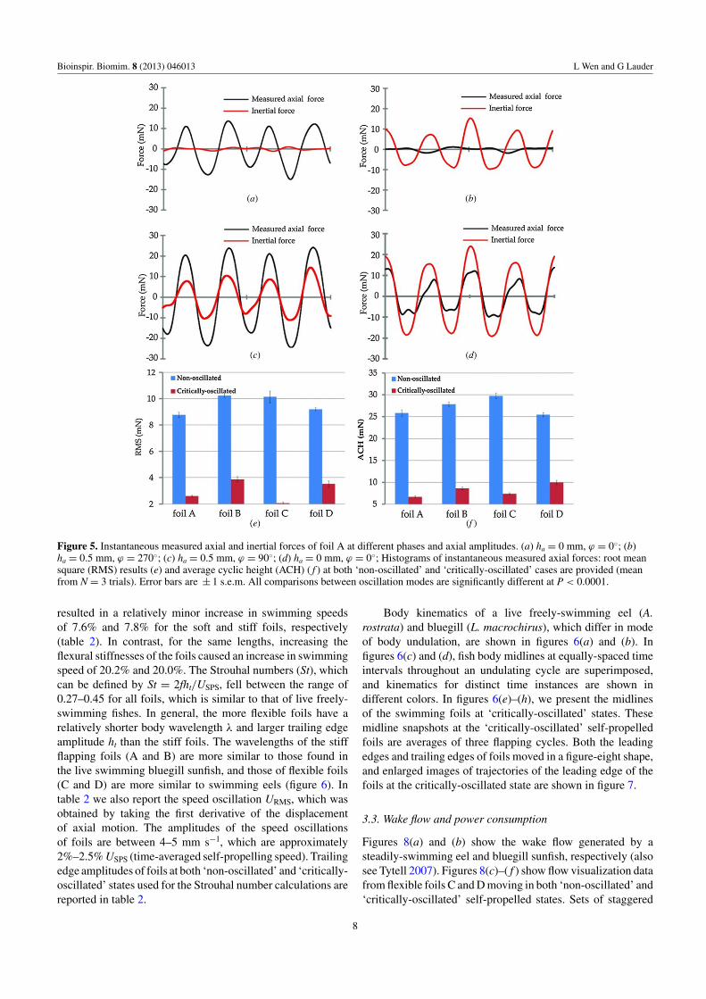
Figure 5. Instantaneous measured axial and inertial forces of foil A at different phases and axial amplitudes. (a) ha = 0 mm, ϕ = 0◦; (b)ha = 0.5 mm, ϕ = 270◦; (c) ha = 0.5 mm, ϕ = 90◦; (d) ha = 0 mm, ϕ = 0◦; Histograms of instantaneous measured axial forces: root meansquare (RMS) results (e) and average cyclic height (ACH) ( f ) at both ‘non-oscillated’ and ‘critically-oscillated’ cases are provided (meanfrom N = 3 trials). Error bars are ± 1 s.e.m. All comparisons between oscillation modes are significantly different at P < 0.0001.

resulted in a relatively minor increase in swimming speedsof 7.6% and 7.8% for the soft and stiff foils, respectively(table 2). In contrast, for the same lengths, increasing theflexural stiffnesses of the foils caused an increase in swimmingspeed of 20.2% and 20.0%. The Strouhal numbers (St), whichcan be defined by St = 2fht/USPS, fell between the range of0.27–0.45 for all foils, which is similar to that of live freely-swimming fishes. In general, the more flexible foils have arelatively shorter body wavelength λ and larger trailing edgeamplitude ht than the stiff foils. The wavelengths of the stiffflapping foils (A and B) are more similar to those found inthe live swimming bluegill sunfish, and those of flexible foils(C and D) are more similar to swimming eels (figure 6). Intable 2 we also report the speed oscillation URMS, which wasobtained by taking the first derivative of the displacementof axial motion. The amplitudes of the speed oscillationsof foils are between 4–5 mm s−1, which are approximately2%–2.5% USPS (time-averaged self-propelling speed). Trailingedge amplitudes of foils at both ‘non-oscillated’ and ‘critically-oscillated’ states used for the Strouhal number calculations arereported in table 2.

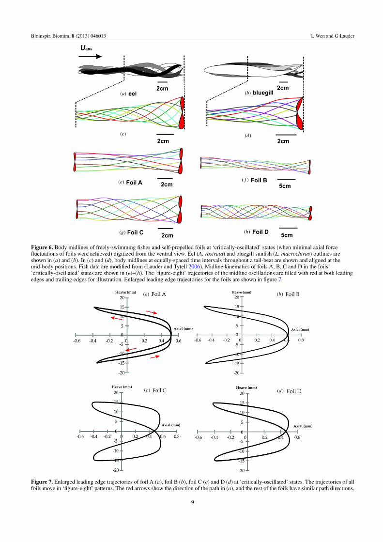
Body kinematics of a live freely-swimming eel (A.rostrata) and bluegill (L. macrochirus), which differ in modeof body undulation, are shown in figures 6(a) and (b). Infigures 6(c) and (d), fish body midlines at equally-spaced timeintervals throughout an undulating cycle are superimposed,and kinematics for distinct time instances are shown indifferent colors. In figures 6(e)–(h), we present the midlinesof the swimming foils at ‘critically-oscillated’ states. Thesemidline snapshots at the ‘critically-oscillated’ self-propelledfoils are averages of three flapping cycles. Both the leadingedges and trailing edges of foils moved in a figure-eight shape,and enlarged images of trajectories of the leading edge of thefoils at the critically-oscillated state are shown in figure 7.

3.3. Wake flow and power consumption

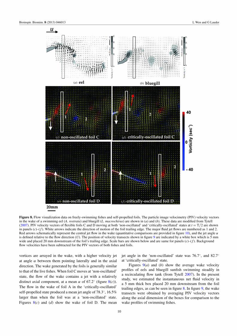
Figures 8(a) and (b) show the wake flow generated by asteadily-swimming eel and bluegill sunfish, respectively (alsosee Tytell 2007). Figures 8(c)–( f ) show flow visualization datafrom flexible foils C and D moving in both ‘non-oscillated’ and‘critically-oscillated’ self-propelled states. Sets of staggered

8

Bioinspir. Biomim. 8 (2013) 046013 L Wen and G Lauder

(a)

(c)

(b)

(d)

(e)

(g) (h)

( f )

Figure 6. Body midlines of freely-swimming fishes and self-propelled foils at ‘critically-oscillated’ states (when minimal axial forcefluctuations of foils were achieved) digitized from the ventral view. Eel (A. rostrata) and bluegill sunfish (L. macrochirus) outlines areshown in (a) and (b). In (c) and (d), body midlines at equally-spaced time intervals throughout a tail-beat are shown and aligned at themid-body positions. Fish data are modified from (Lauder and Tytell 2006). Midline kinematics of foils A, B, C and D in the foils’‘critically-oscillated’ states are shown in (e)–(h). The ‘figure-eight’ trajectories of the midline oscillations are filled with red at both leadingedges and trailing edges for illustration. Enlarged leading edge trajectories for the foils are shown in figure 7.

(a) (b)

(c) (d)

Figure 7. Enlarged leading edge trajectories of foil A (a), foil B (b), foil C (c) and D (d) at ‘critically-oscillated’ states. The trajectories of allfoils move in ‘figure-eight’ patterns. The red arrows show the direction of the path in (a), and the rest of the foils have similar path directions.

9

Bioinspir. Biomim. 8 (2013) 046013 L Wen and G Lauder

(a) (b)

(c) (d )

(e) ( f )

Figure 8. Flow visualization data on freely-swimming fishes and self-propelled foils. The particle image velocimetry (PIV) velocity vectorsin the wake of a swimming eel (A. rostrata) and bluegill (L. macrochirus) are shown in (a) and (b). These data are modified from Tytell(2007). PIV velocity vectors of flexible foils C and D moving at both ‘non-oscillated’ and ‘critically-oscillated’ states at t = T/2 are shownin panels (c)–( f ). White arrows indicate the direction of motion of the foil trailing edge. The major fluid jet flows are numbered as 1 and 2.Red arrows schematically represent the central jet flow in the wake (quantitative comparisons are provided in figure 10), and the jet angle αis defined relative to the flow direction (U). The position of velocity transects shown in figure 9 are indicated by a white box which is 5 mmwide and placed 20 mm downstream of the foil’s trailing edge. Scale bars are shown below and are same for panels (c)–( f ). Backgroundflow velocities have been subtracted for the PIV vectors of both fishes and foils.

vortices are arrayed in the wake, with a higher velocity jetat angle α between them pointing laterally and in the axialdirection. The wake generated by the foils is generally similarto that of the live fishes. When foil C moves at ‘non-oscillated’state, the flow of the wake contains a jet with a relativelydistinct axial component, at a mean α of 67.2◦ (figure 8(c)).The flow in the wake of foil A in the ‘critically-oscillated’self-propelled state produced a mean jet angle of 78.3◦, 16.5%larger than when the foil was at a ‘non-oscillated’ state.Figures 8(c) and (d) show the wake of foil D. The mean

jet angle in the ‘non-oscillated’ state was 76.7◦, and 82.7◦

at ‘critically-oscillated’ state.Figures 9(a) and (b) show the average wake velocity

profiles of eels and bluegill sunfish swimming steadily ina recirculating flow tank (from Tytell 2007). In the presentstudy, we estimated the instantaneous net fluid velocity ina 5 mm thick box placed 20 mm downstream from the foiltrailing edges, as can be seen in figure 8. In figure 9, the waketransects were obtained by averaging PIV velocity vectorsalong the axial dimension of the boxes for comparison to thewake profiles of swimming fishes.

10

Bioinspir. Biomim. 8 (2013) 046013 L Wen and G Lauder

(a) (b)

(c) (d )

(e) ( f )

Figure 9. Transects of average axial wake velocity 10 mm downstream of swimming fishes (a) eel (A. rostrata), and (b) bluegill sunfish(L. macrochirus) (data modified from Tytell 2007), and foils both ‘non-oscillated’ and ‘critically-oscillated’ cases: (c) Foil A; (d) Foil B; (e)Foil C; ( f ) Foil D. The length of the wake profiles of the foils is 150 mm spanning from left to right.

For the stiffer foils (A and B), the mean wake velocitiesin both ‘non-oscillated’ and ‘critically-oscillated’ states arenearly zero. The average wake velocities of foils A and Bshowed profiles that have center peaks with speeds above zero,and two side lobes with speeds below zero. It can be seen infigures 9(c) and (d) that the average wake profiles in bothcases almost overlap. Thus, we speculate that axial oscillationhas very little effect on the wake flow of the stiffer foils usedin the present study. In contrast, the average flow velocityof more flexible foil C in the ‘critically-oscillated’ state wasslightly smaller than that of the foil in the ‘non-oscillated’ state.Interestingly, the mean flow velocity when not oscillated was7.4 mm s−1 larger than when the longer flexible foil (foil D)was oscillated. This result is also reflected in figure 9( f ), wherethe wake profile of foil D is clearly above zero: the averageflow velocity is about 5.7% of the self-propelled speed.

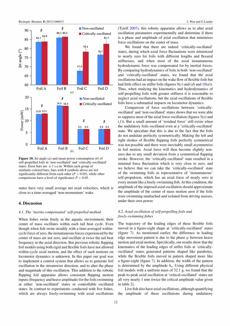
The jet angles of the wakes of foils A to D in both‘non-oscillated’ and ‘critically-oscillated’ states are shown infigure 10(a). The instantaneous wake flows of foils A andB at ‘non-oscillated’ and ‘critically-oscillated’ states are notpresented in figure 8 because they are not significantly differentaccording to the statistical analysis (figure 10(a)).

We also consider how much power Pfoil (see equation (2)for definition) is consumed by the foils. The stiffer foils (A andB) achieved faster self-propelled speeds, but consumed morepower than the flexible foils (C and D). Power consumptionincreases about 28% by increasing the length of the stiff foilsfrom 15 to 30 cm. For the flexible foils, however, power onlyincreased 0.6% as the length doubled. In addition, stiffer foilsconsume more power than the flexible foils. Figure 10(b)shows that the difference in power requirements of foils at‘non-oscillated’ and ‘oscillated’ self-propelled states is smalland not significant, and axial oscillation thus did not affectpower consumption of the swimming foils.

Wake profiles differ considerably among the swimmingfoils, and figure 11 shows the time-averaged flow field offoils A to D in ‘critically-oscillated’ self-propelled states. Theaveraged wake of the short foils (A and C) splits into twojet-like bifurcating streams, with local flow speed slightlygreater than the incoming flow velocity (figures 11(a) and(c)). For longer foils, as shown in figures 11(b) and (d), theaveraged flow field showed a relatively narrow high velocitywake region. In general, the current results demonstrate that thewake flow of the foils at ‘critically-oscillated’ self-propelled

11

Bioinspir. Biomim. 8 (2013) 046013 L Wen and G Lauder

(a)

(b)

Figure 10. Jet angle (a) and mean power consumption (b) ofself-propelled foils in ‘non-oscillated’ and ‘critically-oscillated’states. Error bars are ± 1 s.e.m. Within each group ofsimilarly-colored bars, bars with # symbols above are notsignificantly different from each other (P > 0.05), while othercomparisons have a level of significance P < 0.05.

states have very small average net axial velocities, which isclose to a time-averaged ‘non-momentum’ wake.

4. Discussion

4.1. The ‘inertia-compensated’ self-propelled method

When fishes swim freely in the aquatic environment, theircenter of mass oscillates within each tail beat cycle. Eventhough when fish swim steadily with a time-averaged within-cycle force of zero, the instantaneous forces experienced by thecenter of mass are not zero, and oscillate at twice the tail beatfrequency in the axial direction. But previous robotic flappingfoil models using both rigid and flexible foils have not allowedwithin-cycle axial motion, and the effect of such motions onlocomotor dynamics is unknown. In this paper our goal wasto implement a control system that allows us to generate foiloscillation in the streamwise direction, and to alter the phaseand magnitude of this oscillation. This addition to the roboticflapping foil apparatus allows consistent flapping motioninputs (frequency and heave amplitude) for the foils swimmingin either ‘non-oscillated’ states or controllable oscillatedstates. In contrast to experiments conducted with live fishes,which are always freely-swimming with axial oscillations

(Tytell 2007), this robotic apparatus allows us to alter axialoscillation parameters experimentally and determine if thereis a phase and amplitude of axial oscillation that minimizesforce oscillations on the center of mass.

We found that there are indeed ‘critically-oscillated’states, during which axial force fluctuations were minimizedto nearly zero for foils with different lengths and flexuralstiffnesses, and when most of the axial instantaneoushydrodynamic force was compensated for by inertial forces.By comparing hydrodynamics of foils in both ‘non-oscillated’and ‘critically-oscillated’ states, we found that the axialoscillations had an impact on the wake flow of flexible foils buthad little effect on stiffer foils (figures 9(c) and (d) and 10(a)).Thus, when studying the kinematics and hydrodynamics ofself-propelling foils with greater stiffness it is reasonable toneglect axial oscillations, but the axial oscillations of flexiblefoils have a substantial impacts on locomotor dynamics.

Comparison of force oscillations between ‘critically-oscillated’ and ‘non-oscillated’ states shows that we were ableto suppress most of the axial force oscillation (figures 5(e) and( f )). But a small amount of ‘residual force’ still exists whenthe undulatory foils oscillated even at a ‘critically-oscillated’state. We speculate that this is due to the fact that the foilsdo not undulate perfectly symmetrically. Making the left andright strokes of flexible flapping foils perfectly symmetricalwas not possible and there were inevitably small asymmetriesin foil motion. Axial force will then become slightly non-zero due to any small deviation from a symmetrical flappingstroke. However, the ‘critically-oscillated’ state resulted in aminimal force fluctuation which is very close to zero, andwe believe that we can take the ‘critically-oscillated’ stateof the swimming foils as representative of ‘instantaneous’self-propulsion, which has an axial force of nearly zero atevery instant like a freely-swimming fish. At this condition, theamplitude of the imposed axial oscillation should approximatethe amplitude of the center of mass motion seen if the foilswere swimming unattached and isolated from driving masses,under their own power.

4.2. Axial oscillation of self-propelling foils andfreely-swimming fishes

The trajectory of the leading edges of these flexible foilsmoved in a figure-eight shape at ‘critically-oscillated’ states(figure 7). As mentioned earlier, the difference in leadingedge movement pattern is due to the phase ϕ between heavemotion and axial motion. Specifically, our results show that thekinematics of the leading edges of stiffer foils at ‘critically-oscillated’ states generated patterns shaped like parabolas,while the flexible foils moved in pattern shaped more likea figure-eight (figure 7). In addition, the width of the patternis determined by the amplitude ha. Using different physicalfoil models with a uniform mass of 32.1 g, we found that thepeak-to-peak axial oscillation at ‘critical-oscillated’ states areall very nearly 1 mm (twice the critical amplitude value givenin table 2).

Live fish also have axial oscillations, although quantifyingthe amplitude of these oscillations during undulatory

12

Bioinspir. Biomim. 8 (2013) 046013 L Wen and G Lauder

(b)(a)

(d )(c)

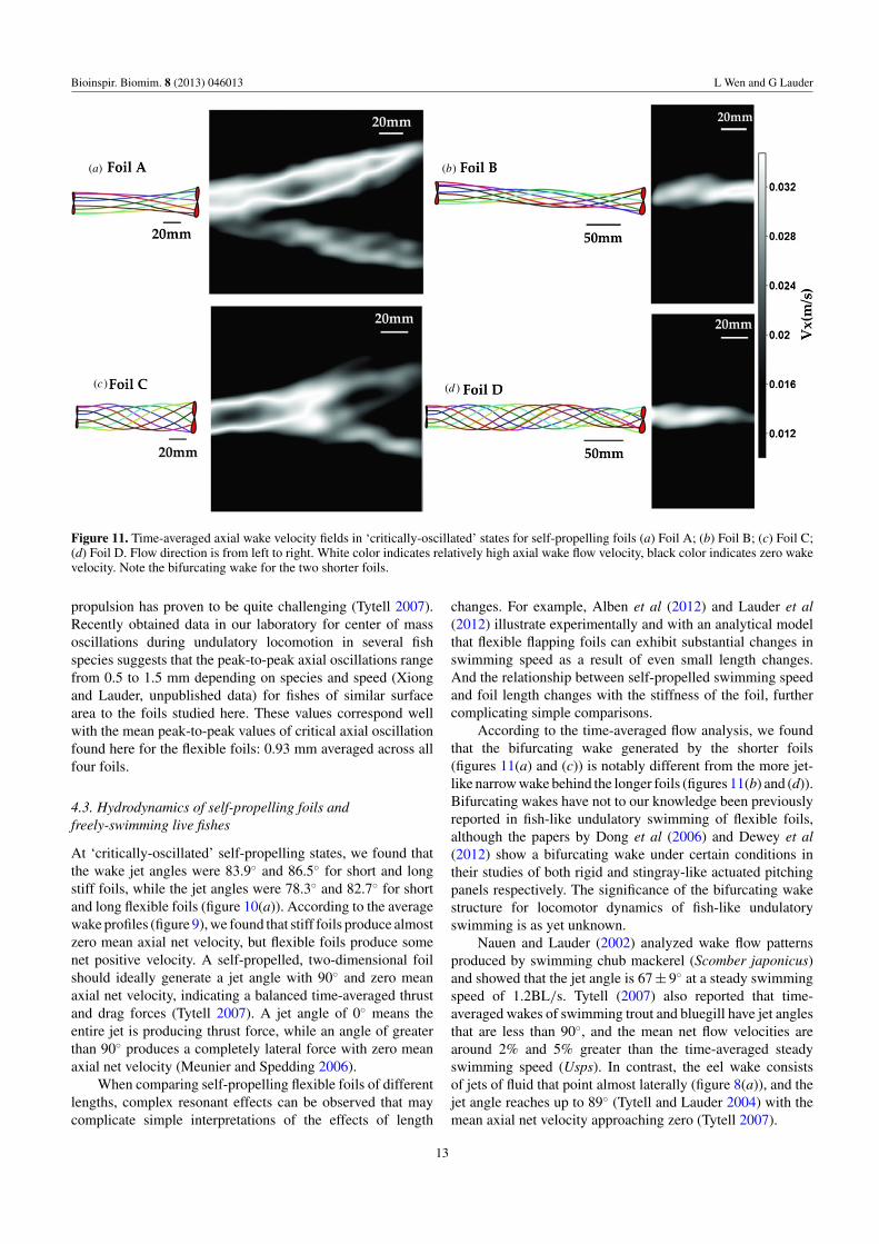
Figure 11. Time-averaged axial wake velocity fields in ‘critically-oscillated’ states for self-propelling foils (a) Foil A; (b) Foil B; (c) Foil C;(d) Foil D. Flow direction is from left to right. White color indicates relatively high axial wake flow velocity, black color indicates zero wakevelocity. Note the bifurcating wake for the two shorter foils.

propulsion has proven to be quite challenging (Tytell 2007).Recently obtained data in our laboratory for center of massoscillations during undulatory locomotion in several fishspecies suggests that the peak-to-peak axial oscillations rangefrom 0.5 to 1.5 mm depending on species and speed (Xiongand Lauder, unpublished data) for fishes of similar surfacearea to the foils studied here. These values correspond wellwith the mean peak-to-peak values of critical axial oscillationfound here for the flexible foils: 0.93 mm averaged across allfour foils.

4.3. Hydrodynamics of self-propelling foils andfreely-swimming live fishes

At ‘critically-oscillated’ self-propelling states, we found thatthe wake jet angles were 83.9◦ and 86.5◦ for short and longstiff foils, while the jet angles were 78.3◦ and 82.7◦ for shortand long flexible foils (figure 10(a)). According to the averagewake profiles (figure 9), we found that stiff foils produce almostzero mean axial net velocity, but flexible foils produce somenet positive velocity. A self-propelled, two-dimensional foilshould ideally generate a jet angle with 90◦ and zero meanaxial net velocity, indicating a balanced time-averaged thrustand drag forces (Tytell 2007). A jet angle of 0◦ means theentire jet is producing thrust force, while an angle of greaterthan 90◦ produces a completely lateral force with zero meanaxial net velocity (Meunier and Spedding 2006).

When comparing self-propelling flexible foils of differentlengths, complex resonant effects can be observed that maycomplicate simple interpretations of the effects of length

changes. For example, Alben et al (2012) and Lauder et al(2012) illustrate experimentally and with an analytical modelthat flexible flapping foils can exhibit substantial changes inswimming speed as a result of even small length changes.And the relationship between self-propelled swimming speedand foil length changes with the stiffness of the foil, furthercomplicating simple comparisons.

According to the time-averaged flow analysis, we foundthat the bifurcating wake generated by the shorter foils(figures 11(a) and (c)) is notably different from the more jet-like narrow wake behind the longer foils (figures 11(b) and (d)).Bifurcating wakes have not to our knowledge been previouslyreported in fish-like undulatory swimming of flexible foils,although the papers by Dong et al (2006) and Dewey et al(2012) show a bifurcating wake under certain conditions intheir studies of both rigid and stingray-like actuated pitchingpanels respectively. The significance of the bifurcating wakestructure for locomotor dynamics of fish-like undulatoryswimming is as yet unknown.

Nauen and Lauder (2002) analyzed wake flow patternsproduced by swimming chub mackerel (Scomber japonicus)and showed that the jet angle is 67 ± 9◦ at a steady swimmingspeed of 1.2BL/s. Tytell (2007) also reported that time-averaged wakes of swimming trout and bluegill have jet anglesthat are less than 90◦, and the mean net flow velocities arearound 2% and 5% greater than the time-averaged steadyswimming speed (Usps). In contrast, the eel wake consistsof jets of fluid that point almost laterally (figure 8(a)), and thejet angle reaches up to 89◦ (Tytell and Lauder 2004) with themean axial net velocity approaching zero (Tytell 2007).

13

Bioinspir. Biomim. 8 (2013) 046013 L Wen and G Lauder

Why are wake jet angles not 90◦ and why does a positivemean axial net velocity exist for freely-swimming live fishes(except eels) and the robotic foils studied here? We speculatethat it is possibly due to the fact that there might be acontribution to the net thrust force produced by the undulatoryanterior part of the fish or flexible foils. For example, leadingedge suction on the body or fins can contribute substantiallyto trust and has been demonstrated previously in flexiblefoil propulsion (Borazjani and Daghooghi 2013, Oeffner andLauder 2012). In addition, complicated three-dimensionaleffects arising from the fins and body edges above and belowthe laser plane in which flows are visualized here almostcertainly play a role in contributing to the wake flow field andmomentum transfer from the fish or foil to the fluid. To betterunderstand this issue, further numerical and experimentalthree-dimensional flow analyses around both freely-swimminglive fish and robotic foil models are needed (e.g., Borazjani andDaghooghi 2013, Flammang et al 2011).

One noteworthy aspect of the self-propelling passivelyflexible foils is that their kinematics closely approximatethe posterior thrust producing region of undulatory fishlocomotion (e.g., figure 6). We believe that there are severalreasons for this. First, during slow to moderate swimmingspeeds, fish activate only red muscle fibers which make uponly a small fraction (less than 10%) of the fish’s muscle mass.Most of the body, composed of myotomal white fibers, is thusacting passively. Second, during a number of fish swimmingbehaviors, including locomotion behind bluff bodies that sheda Karman vortex street, fish can generate thrust with a passiveflexible body (Beal et al 2006, Liao et al 2003a, 2003b), andpassive body dynamics are critical to swimming in the Karmanvortex street. Third, over a wide range of swimming speeds,the anterior body region of swimming fish undergoes minimalheave motion, and it is the posterior body that is the thrustgenerating region (Lauder and Tytell 2006). This area is thuswell modeled by a flapping flexible foil that generates thrustas a result of heave motion at its leading edge, and the passiveflexible foils studied here show curvatures that are similar tothose of freely-swimming fishes.

5. Conclusions

We provide an analysis of the swimming performance ofundulating passive robotic foils with axial oscillation thatis biologically relevant to freely-swimming fish by flappingplastic foils with two different lengths and two stiffnesses.We found ‘critically-oscillated’ states for each foil when theaxial force fluctuation reached a minimum, and when mostof the instantaneous hydrodynamic forces were compensatedby inertial forces. While at ‘critically-oscillated’ states, thefoils with biologically relevant heave parameters resulted in∼1 mm total oscillation in the axial direction, similar torecently obtained results on center of mass oscillations fromfreely-swimming fishes. At ‘critically-oscillated’ states, theleading edge patterns of flexible foils are figure-eight-shaped,while the motion of the leading edge of stiffer foils is shapedmore like a parabola. From flow visualization analyses, somedifferences in wake flow patterns were observed in flexible

foils between the ‘critically-oscillated’ and ‘non-oscillated’states. Axial oscillation thus affects swimming hydrodynamicsof flexible bodies, but has much less effect on stiff foils.

The addition of a mechanism that generates controlledaxial oscillations to current robotic foil systems provides anew experimental avenue for studying the dynamics of self-propelled swimming in flexible bodies.

Acknowledgments

This work was supported by NSF grant EFRI-0938043. Wethank members of the Lauder and James Tangorra Labs (DrexelUniversity) for many helpful discussions on fish fins andflexible flapping foil propulsion, Silas Alben for assistancein interpreting flapping foil results, Eric Tytell for manydiscussions on wake flow patterns, Dan Quinn for discussingthe force and wake results, Erik Anderson, Vern Baker, andChuck Witt for their considerable efforts in designing therobotic flapper and control software, and Erin Blevins andGabe Walker for improving the paper.

References

Alben S, Witt C, Baker T V, Anderson E J and Lauder G V 2012Dynamics of freely swimming flexible foils Phys. Fluids A24 051901

Anderson J M, Streitlien K and Barrett D S 1998 Oscillating foils ofhigh propulsive efficiency J. Fluid Mech. 360 41–72

Barrett D S, Triantafyllou M S and Yue D P 1999 Drag reduction infish-like locomotion J. Fluid Mech. 392 183–212

Beal D N, Hover F S, Triantafyllou M S, Liao J and Lauder G V2006 Passive propulsion in vortex wakes J. Fluid Mech.549 385–402

Blevins E and Lauder G V 2013 Swimming near the substrate: asimple robotic model of stingray locomotion Bioinspir.Biomim. 8 016005

Borazjani I and Daghooghi M 2013 The fish tail motion forms anattached leading edge vortex Proc. R. Soc. Lond. Biol. Sci.280 20122071

Borazjani I and Sotiropoulos F 2008 Numerical investigation of thehydrodynamics of carangiform swimming in the transitionaland inertial flow regimes J. Exp. Biol. 211 1541–58

Borazjani I and Sotiropoulos F 2009 Numerical investigation of thehydrodynamics of anguilliform swimming in the transitionaland inertial flow regimes J. Exp. Biol. 212 576–92

Buchholz J H and Smits A J 2008 The wake structure and thrustperformance of a rigid low-aspect-ratio pitching panel J. FluidMech. 603 331–65

Dewey P A, Carriou A and Smits A J 2012 On the relationshipbetween efficiency and wake structure of a batoid-inspiredoscillating fin J. Fluid Mech. 691 245–66

Dong H, Mittal R and Najjar F M 2006 Wake topology andhydrodynamic performance of low aspect-ratio flapping foilsJ. Fluid Mech. 566 309–43

Drucker E G and Lauder G V 1999 Locomotor forces on aswimming fish: three-dimensional vortex wake dynamicsquantified using digital particle image velocimetry J. Exp. Biol.202 2393–412

Fish F, Nusbaum M, Beneski J and Ketten D 2006 Passivecambering and flexible propulsors: cetacean flukes Bioinspir.Biomim. 1 S42–8

Flammang B E, Lauder G V, Troolin D R and Strand T 2011Volumetric imaging of fish locomotion Biol. Lett. 7 695–98

Kern S and Koumoutsakos P 2006 Simulations of optimizedanguilliform swimming J. Exp. Biol. 209 4841–57

14

Bioinspir. Biomim. 8 (2013) 046013 L Wen and G Lauder

Lauder G V 2011 Swimming hydrodynamics: ten questions and thetechnical approaches needed to resolve them Exp. Fluids51 23–35

Lauder G V, Anderson E J, Tangorra J and Madden P G A 2007Fish biorobotics: kinematics and hydrodynamics ofself-propulsion J. Exp. Biol. 210 2767–80

Lauder G V, Flammang B E and Alben S 2012 Passive roboticmodels of propulsion by the bodies and caudal fins of fishIntegr. Comp. Biol. 52 576–87

Lauder G V, Lim J, Shelton R, Witt C, Anderson E and Tangorra J L2011a Robotic models for studying undulatory locomotion infishes Mar. Technol. Soc. J. 45 41–55

Lauder G V and Madden P G A 2006 Learning from fish:kinematics and experimental hydrodynamics for roboticists Int.J. Automat. Comput. 4 325–35

Lauder G V, Madden P G, Tangorra J L, Anderson E and Baker T V2011b Bioinspiration from fish for smart material design andfunction Smart Mater. Struct. 20 094014

Lauder G V and Tytell E D 2006 Hydrodynamics of undulatorypropulsion Fish Biomechanics. Volume 23 in Fish Physiologyed R E Shadwick and G V Lauder (San Diego, CA: Academic)pp 425–68

Liao J, Beal D N, Lauder G V and Triantafyllou M S 2003a TheKarman gait: novel body kinematics of rainbow troutswimming in a vortex street J. Exp. Biol. 206 1059–73

Liao J C, Beal D N, Lauder G V and Triantafyllou M S 2003b Fishexploiting vortices decrease muscle activity Science302 1566–9

Long J, Koob-Emunds M, Sinwell B and Koob T J 2002 Thenotochord of hagfish Myxine glutinosa: visco-elastic propertiesand mechanical functions during steady swimming J. Exp.Biol. 205 3819–31

Low K H and Chong C W 2010 Parametric study of the swimmingperformance of a fish robot propelled by a flexible caudal finBioinspir. Biomim. 5 046002

McHenry M J, Pell C A and Long J H 1995 Mechanical control ofswimming speed: stiffness and axial form in undulating fishmodels J. Exp. Biol. 198 2293–305

Meunier P and Spedding G R 2006 Stratified propeller wakesJ. Fluid Mech. 552 229–56

Nauen J C and Lauder G V 2002 Hydrodynamics of caudal finlocomotion by chub mackerel, Scomber japonicus(Scombridae) J. Exp. Biol. 205 1709–24

Oeffner J and Lauder G V 2012 The hydrodynamic function ofshark skin and two biomimetic applications J. Exp. Biol.215 785–95

Read D A, Hover F S and Triantafyllou M S 2003 Forces onoscillating foils for propulsion and maneuvering J. FluidStruct. 17 163–83

Sun M and Wu J H 2003 Aerodynamic force generation and powerrequirements in forward flight in a fruit fly with modeled wingmotion J. Exp. Biol. 206 3065–83

Techet A H 2008 Propulsive performance of biologically inspiredflapping foils at high Reynolds numbers J. Exp. Biol.211 274–79

Triantafyllou M S 2005 Review of hydrodynamic scaling laws inaquatic locomotion and fish-like swimming Appl. Mech. Rev.58 226–38

Triantafyllou M S, Triantafyllou G S and Yue D P 2000Hydrodynamics of fishlike swimming Ann. Rev. Fluid Mech.32 33–53

Tytell E D 2007 Do trout swim better than eels? Challenges forestimating performance based on the wake of self-propelledbodies Exp. Fluids 43 701–12

Tytell E D, Hsu C Y, Williams T L, Cohen A H and Fauci L J2010 Interactions between body stiffness, muscle activation,and fluid environment in a neuromechanical model of lampreyswimming Proc. Natl Acad. Sci. 107 19832–7

Tytell E D and Lauder G V 2004 The hydrodynamics of eelswimming: I. Wake structure J. Exp. Biol. 207 1825–41

Walker J A 2004 Dynamics of pectoral fin rowing in a fish with anextreme rowing stroke: the threespine stickleback(Gasterosteus aculeatus) J. Exp. Biol. 207 1925–39

Walker J A and Westneat M W 1997 Labriform propulsionin fishes: kinematics of flapping aquatic flight inthe bird wrasse Gomphosus varius (Labridae) J. Exp. Biol.200 1549–69

Wen L, Wang T M, Wu G H and Liang J H 2012 Hydrodynamicinvestigation of a self-propulsive robotic fish based on aforce-feedback control method Bioinspir. Biomim. 7 036012

15