underwater acoustic barriers experiment uab’07 part a: the

CINTAL - Centro de Investigacao Tecnologica do Algarve

Universidade do Algarve

Underwater Acoustic Barriers Experiment

UAB’07 Part A: the Hopavagen Bay

S.M. Jesus, A. Silva, C. Martins and F. Zabel

Rep 05/07 - SiPLAB15/December/2007

University of Algarve tel: +351-289800131Campus de Gambelas fax: +351-2898642588005-139, Faro [email protected] www.ualg.pt/cintal

Work requested by CINTAL - Centro de Investigacao Tecnologica do AlgarveCampus de Gambelas, Universidade do Algarve8005-139 Faro, PortugalTel: +351-289800131, fax: [email protected], www.ualg.pt/cintal/

Laboratory performing SiPLAB - Signal Processing Laboratorythe work Universidade do Algarve, FCT, Campus de Gambelas,

8005-139 Faro, Portugaltel: +351-289800949, fax: [email protected], www.siplab.fct.ualg.pt/

Projects UAB (POCI/MAR/59008/2004)Title Underwater Acoustic Barriers (UAB’07) Experiment

Part A: the Hopavagen BayAuthors S.M.Jesus, A. Silva, C. Martins, F. ZabelDate December 15, 2007Reference 05/07 - SiPLABNumber of pages 41 (forty one)Abstract This report describes the data acquired during the

UAB’07 experiment. Part A describes the data setacquired at the Hopavagen Bay in Norway, from 11 to 13September 2007.

Clearance level UNCLASSIFIEDDistribution list NTNU(1), SiPLAB(1), CINTAL (1)Total number of copies 3 (three)

Copyright Cintal@2007

III

Foreword and Acknowledgment

This report presents the data acquired with one Acoustic Oceanographic Buoy (AOB)system and the preliminary results obtained during the UAB’07 sea trial, that took placein the bay of Trondheim and at the Hopavagen Bay (Norway), during the period Septem-ber 3 - 14, 2007. Part A concentrates in the description of the experiment conducted atthe Hopavagen Bay.

The authors of this report would like to thank:

• all the personnel involved and in particular Alexandra Neyts and Jens Hovem fromNTNU for their collaboration and interest on this experiment,

• FCT (Portugal) for the funding provided under projects UAB (POCI/MAR/59008/2004)and RADAR (POCTI/CTA/47719/2002) (AOB equipment).

The work described in this report was supported by the European Community’s SixthFramework Programme through the grant to the budget of the Integrated InfrastructureInitiative HYDRALAB III, Contract no. 022441 (RII3).

IV

intentionally blank

Contents

List of Figures VI

1 Introduction 11

2 The UAB’07 sea trial 132.1 Generalities and sea trial area . . . . . . . . . . . . . . . . . . . . . . . . . 132.2 Ground truth measurements . . . . . . . . . . . . . . . . . . . . . . . . . . 14

2.2.1 Archival environmental data . . . . . . . . . . . . . . . . . . . . . . 142.2.2 Seafloor information . . . . . . . . . . . . . . . . . . . . . . . . . . 152.2.3 Water column and surface data . . . . . . . . . . . . . . . . . . . . 15

2.3 Deployment geometries in the Hopavagen Bay . . . . . . . . . . . . . . . . 182.3.1 Acoustic source array . . . . . . . . . . . . . . . . . . . . . . . . . . 182.3.2 AOB geometry: depth and range . . . . . . . . . . . . . . . . . . . 19

3 Acoustic data 233.1 Emitted signals . . . . . . . . . . . . . . . . . . . . . . . . . . . . . . . . . 243.2 Signal generator and amplifier . . . . . . . . . . . . . . . . . . . . . . . . . 253.3 Acoustic sources . . . . . . . . . . . . . . . . . . . . . . . . . . . . . . . . . 253.4 Received signals . . . . . . . . . . . . . . . . . . . . . . . . . . . . . . . . . 26

3.4.1 Data format . . . . . . . . . . . . . . . . . . . . . . . . . . . . . . . 263.4.2 Channel selection and summation . . . . . . . . . . . . . . . . . . . 263.4.3 The 4 by 4 repetition problem . . . . . . . . . . . . . . . . . . . . . 273.4.4 Day 254 (September 11, 2007) . . . . . . . . . . . . . . . . . . . . . 283.4.5 Day 255 (September 12, 2007) . . . . . . . . . . . . . . . . . . . . . 303.4.6 Day 256 (September 13, 2007) . . . . . . . . . . . . . . . . . . . . . 31

3.5 Signal detection . . . . . . . . . . . . . . . . . . . . . . . . . . . . . . . . . 33

4 Conclusions and future analysis 37

A Data reading routine: readlocapassdata.m 39

V

List of Figures

2.1 UAB experiment area in the Hopavagen bay map. . . . . . . . . . . . . . . 13

2.2 Mean temperature and salinity profiles from archival data for the month ofSeptember of the last 10 years (1996 - 2006) for the Hopavagen bay. . . . . 14

2.3 Bathymetry recording of the Hopavagen bay (courtesy of NTNU / Bates [1]). 15

2.4 AOB22 thermistor string data for day 254 unfiltered (a) and lowpass filtered(b). . . . . . . . . . . . . . . . . . . . . . . . . . . . . . . . . . . . . . . . . 16

2.5 low-pass filtered AOB22 temperature profiles from thermistor string datafor the first 10 minutes of day 254; thick line is the mean temperature profile. 17

2.6 first three EOF’s computed from thermistor chain data during the Hopavagenbay part of the UAB07 experiment. . . . . . . . . . . . . . . . . . . . . . . 17

2.7 Hobo autonomous recording water depth (top) and temperature (bottom),near the pier to infer tidal variation in the bay. . . . . . . . . . . . . . . . 18

2.8 AOB and source moorings at the Hopavagen Bay. . . . . . . . . . . . . . . 18

2.9 sketch of the source array mooring and configuration. . . . . . . . . . . . . 19

2.10 sketch of the AOB folded receiver array during the mooring at Sletvik. . . . 19

2.11 AOB22 GPS position during the Hopavagen bay deployments of days 11,12 and 13 of September, 2007: source position (red square), mean arraypoistion (black square), one standard deviation on GPS position of receivingarray (thick circle), mean acoustic barrier position (green line). . . . . . . 21

2.12 AOB22 GPS estimated source range variations along time for days 11, 12and 23 September, 2007. . . . . . . . . . . . . . . . . . . . . . . . . . . . . 22

2.13 Day 256, September 13, 2008: target GPS estimated position (a), sourcedepth (b) and source - target range (c). . . . . . . . . . . . . . . . . . . . . 22

3.1 experimental setup for signal control and processing during the Hopavagenbay experiment. . . . . . . . . . . . . . . . . . . . . . . . . . . . . . . . . . 23

3.2 Time - frequency sketch of the typical transmit sequence. . . . . . . . . . . 24

3.3 Signal generation system used during the Hopavagen bay phase of UAB07. . 25

VI

LIST OF FIGURES VII

3.4 Lubell 916C sound source (a) and transmitt voltage response - TVR (b). . . 25

3.5 Day 254 14:12 UTC: pulse compression of all channels with LFM upsweep0.2 s duration in the band LF band: 3500 - 6500 Hz. . . . . . . . . . . . . 27

3.6 Day 254 14:12 UTC: pulse compression of channels 1, 5, 9 and 13 at re-spective depths of 6.6, 22.6, 7.7 and 13.7 meter [LF upsweep 0.2 s durationin the LF band: 3500-6500 Hz]. . . . . . . . . . . . . . . . . . . . . . . . . 28

3.7 Day 254: OFDM communication signals for source testing as received onhydrophone 1 (6.6 m depth). . . . . . . . . . . . . . . . . . . . . . . . . . . 29

3.8 Day 254 hydrophone 1 (6.6 m depth): up - down sweeps in the lower 5 kHzband and corresponding harmonics. . . . . . . . . . . . . . . . . . . . . . . 30

3.9 Day 254, hydrophone 1 (6.6 m depth): arrival pattern for the 3 kHz bandup sweep along time (a) and mean arrival pattern (b). . . . . . . . . . . . . 30

3.10 Day 255 hydrophone 5 at 22.6 m depth, 0.5 s LFM sweeps in the 7.5 - 10.5kHz band, start time 10:31 UTC: time variability (a) and mean arrivalpattern (b). . . . . . . . . . . . . . . . . . . . . . . . . . . . . . . . . . . . 31

3.11 Day 256 impulse responses between sound source at 3 m depth (S1) andeach hydrophone for frequency bands : 3500 - 6500 Hz (a), 7500 - 10500Hz (b) and 12000 - 15500 Hz (c). . . . . . . . . . . . . . . . . . . . . . . . 34

3.12 Day 256 hydrophone 4 at 13:27 UTC as a summation of several channelsaccording to the tabel above: time - frequency (left) and time compressedtime series (left), source 1 (a) and source 2 (b). . . . . . . . . . . . . . . . 35

3.13 Day 256 correlations with HF downsweep pulse starting at 16:01 UTC forchannels: 1 at 6.6 m depth (a), 9 at 7.7 m depth (b), 13 at 13.7 m depth(c) and 5 at 22.6 m depth (d). Signal transmission was interrupted andre-initialized at 16:18 UTC. Horizontal lines mark the target crossings ofthe virtual barrier according to measured time of table 2.3. . . . . . . . . . 36

VIII LIST OF FIGURES

intentionally blank

Abstract

The project Underwater Acoustic Barriers (UAB) started in 2006 with the objective ofproving the concept of using underwater sound propagation to detect submerged objectscrossing a given area. The UAB project involved three phases: i) a theoretical study,ii) a system development and iii) at sea testing. The first two phases are respectivelycovered in [2] and [3, 4] and other future publications while this report concentrates onthe testing at sea. The experimental testing of the UAB concept involves establishingan acoustic propagation plane (barrier) normally in a relatively shallow area (20-30 mdepth) of a bay or port, while the equipment itself is connected to the nearby shore. Forthe purpose of this first testing it is important to perform the experiment in a relativelyquiet and environmentally well controlled area, in order to avoid interfering noises andrapidly changing environmental conditions. These conditions are relatively difficult tofind in Portugal with its long open ocean coast and too shallow semi-enclosed bays orriver estuaries therefore decision was made to apply for performing this experiment at theTrondheim Research Infrastructure Facility (Hydralab III). The experiment took place attwo different sites: the Trondheimsfjord / Trondheim Biological Station (TBS) using theR/V Gunnerus and at the Sletvik Field Station (Hopavagen bay) in the periods September3 - 7 and 8 - 14, respectively. This part A of the report describes the data set acquiredat the bay of Hopavagen during which both the acoustic source array and the receivingarray were moored at an approximate range of 100 m, creating a virtual acoustic barrier.

9

10 LIST OF FIGURES

intentionally blank

Chapter 1

Introduction

In the period after the 9/11 attacks the international community became aware of thenecessity to protect critical areas from threats resulting from potential terrorist intrusion.Comercial and military ports, bays, straits and other coastal areas with industrial/energyplants are part of vital infrastructures that maybe targeted by terrorist groups. Land andair attacks are normally accounted for by traditional radars, infrared and other electro-magnetic means while underwater threats are much more difficult to detect in practicalsituations. Standard low frequency sonars are normally suited for long range deep watertarget detection and are therefore not adapted to the detection of possible small objectssuch as autonomous underwater vehicles (AUV) or divers in enclosed very shallow waterbays or river estuaries. Therefore new techniques need to be developed for that partic-ular task of detecting small (say down to a meter size) objects moving at low speed inbetween two points, say, 500 m apart, at the entrance of the area to protect. The areaitself is composed of a water layer varying between 10 and 40 m, and may be subject tostrong acoustic noise interference as is common in a sea port with the frequent passageof commercial and fishing vessels.

There are a number of possible approaches for this task as for example the lay downof bottom upward looking acoustic transducers creating a virtual barrier much similar tothe technique used in acoustic current profiling (ADCP), or a forward looking set of highfrequency acoustic transducers. A common feature of all these approaches is that theyare based on the detection of the target backscatter and therefore highly dependent onthe target material, size, aspect and acoustic reflectivity which, we know, can be verydefavorable in the case of a diver, for instance. A different concept applies to the settingof an acoustic barrier between two line arrays, one on each side of the entrance of thearea to be protected: one side emmits signals and the other receives signals. In thatcase the target is possibly detected by its forward scatterer, i.e., its ability to perturbthe permanent acoustic field created between the two line arrays. It is this perturbationthat creates the detection. Of course the field perturbation still depends on the physicalcharacteristics of the target, such as size, cross-section, acoustic impedance and so on, butit is anticipated that much smaller targets can be detected by detecting field perturbation/ foreward scattering than based on the backward scatered energy.

The project Underwater Acoustic Barriers (UAB) was proposed to the Fundacao para aCiencia e a Tecnologia (FCT) under the POCI program in the open call of 2004, approvedin 2005 and started in 2006 with the objective of proving the concept of using underwatersound propagation to detect submerged objects crossing a given area. The UAB projectinvolved three phases: i) a theoretical study, ii) a system development and iii) at sea

11

12 CHAPTER 1. INTRODUCTION

testing. The first two phases are respectively covered in [2] and [3, 4] and other futurepublications while this report concentrates on the testing at sea. The experimental testingof the UAB concept involves establishing an acoustic propagation plane (barrier) in agenerally relatively shallow area (20-30 m depth) of a bay or port, while the equipmentitself is connected to the nearby shore. For the purpose of this first testing it is importantto perform the experiment in a relatively quiet and environmentally well controlled area,in order to avoid interfering noises and rapidly changing conditions. These conditionsare relatively difficult to find in Portugal with its long open ocean coast and too shallowsemi-enclosed bays or river estuaries therefore decision was made to apply for performingthis experiment at the Trondheim Research Infrastructure Facility (Hydralab III). Theexperiment took place at two different sites: the Trondheimsfjord / Trondheim BiologicalStation (TBS) (R/V Gunnerus) and at the Sletvik Field Station (Hopavagen) in theperiods September 3 - 7 and 8 - 14, respectively. During the TBS part of the experimentsignals were transmitted from the TBS peer using one or various acoustic high frequencysources to the receiving buoy (AOB) deployed using the R/V Gunnerus in a free driftingconfiguration, while during the second part, in Sletvik, both the acoustic source arrayand the receiving array were moored in the Hopavaagen bay at an approximate rangeof 100 m, creating a virtual acoustic barrier. This report describes only the data setacquired during the second part of the experiment, at the Hopavagen Bay wich purposewas to test the effective target detection capacity of an acoustic barrier in a semi-enclosedunperturbated area.

The present document aims at providing as much as possible a complete report of thevarious acoustic data sets acquired during the UAB’07 experiment as well as accompany-ing relevant information such as ship’s and buoy’s/array’s position, currents, temperatureprofiles, geo-acoustic information and other concurrent remote sensing data. This reportis organized as follows: section 2 describes the sea trial itself with various archival datasets, bathymetry, geometries and environment information recorded during the experi-ment; section 2.3 makes a short description of the experimental setup and deploymentgeometries; section 3 describes the recorded acoustic data as well as all relevant informa-tion regarding signal transmission and preliminary results on the received data. Finally,section 4 concludes this report giving some hints about most interesting sets for posteriorprocessing and/or future experiments.

Chapter 2

The UAB’07 sea trial

2.1 Generalities and sea trial area

The selected area for the Hopavagen bay part of the UAB’07 experiment is shown in figure2.1. This area is interesting for the purpose of this experiment for the following reasons:

Figure 2.1: UAB experiment area in the Hopavagen bay map.

• it is an enclosed well protected bay from winds and waves,

• it has no ship trafic at all,

• equipment can be left deployed and unattended for hours and days with no or verysmall risk,

• water depths are ideal for testing the UAB concept: between 8 and 30 m.

During the experiment, the bay was very calm, sea state 0 all days due to the naturalbay protection with some 20/30 knot wind during day September 12 and 5 knot the other

13

14 CHAPTER 2. THE UAB’07 SEA TRIAL

days. A few thermistor chain measurements were made using an AOB included thermistorstring (see 2.2.3.1).

A small outboard engine boat was used to deploy the two source array, that was leftout during the whole experiment, and the AOB that was anchored approximately 100 maway and that was recovered every day in order to allow battery charging and full datadownloading. Data transmission and reception was controlled from a base station closeto the small pier used for accessing the small boat, via cable for the sound source arrayand via wireless for the AOB. Due to the time required for equipment preparation andmooring and then recovering, the actual data transmissions lasted for three entire daysfrom 11 to 13 of September and are described below.

2.2 Ground truth measurements

The ground truth was relatively sparse and limited to archival data and some thermistorchain measurements. Bottom knowledge was limited to historical information.

2.2.1 Archival environmental data

Archival data of temperature and salinity profiles for the Hopavaagen bay are shown infigure 2.2. These are mean profiles obtained during the month of September in the yearsfrom 1996 and 2006 (courtesy of Alexandra Neyts, NTNU).

Figure 2.2: Mean temperature and salinity profiles from archival data for the month ofSeptember of the last 10 years (1996 - 2006) for the Hopavagen bay.

2.2. GROUND TRUTH MEASUREMENTS 15

2.2.2 Seafloor information

The bottom of the Hopavagen bay is traditionally described as being made of sand inmost of the area (that has a depth of about 20 m). In the deepest parts of the bay(about 30 m), the bottom is more muddy, with some organic marine sediments. There,the bottom may be anoxic during parts of the summer. A complementary informationabout that area can be obtained from Bates [1], that performed a complete survey of thearea using an echosounder system coupled with an additional processing for extractingbottom type information. The results show a variable bottom structure around the baywith a prodominance of fine sand to mud / silt in the deeper areas where acoustic signalswere transmitted. This information was checked against ground truth coring.

2.2.2.1 Bathymetry

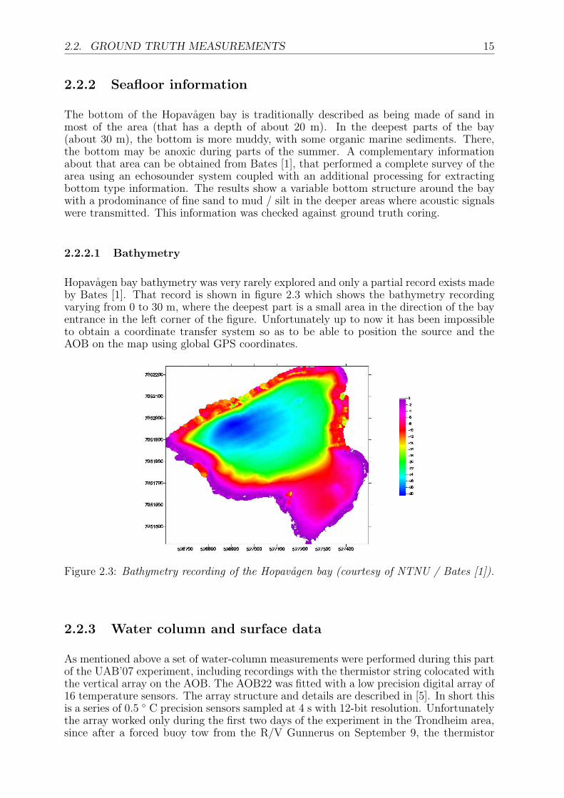
Hopavagen bay bathymetry was very rarely explored and only a partial record exists madeby Bates [1]. That record is shown in figure 2.3 which shows the bathymetry recordingvarying from 0 to 30 m, where the deepest part is a small area in the direction of the bayentrance in the left corner of the figure. Unfortunately up to now it has been impossibleto obtain a coordinate transfer system so as to be able to position the source and theAOB on the map using global GPS coordinates.

Figure 2.3: Bathymetry recording of the Hopavagen bay (courtesy of NTNU / Bates [1]).

2.2.3 Water column and surface data

As mentioned above a set of water-column measurements were performed during this partof the UAB’07 experiment, including recordings with the thermistor string colocated withthe vertical array on the AOB. The AOB22 was fitted with a low precision digital array of16 temperature sensors. The array structure and details are described in [5]. In short thisis a series of 0.5 ◦ C precision sensors sampled at 4 s with 12-bit resolution. Unfortunatelythe array worked only during the first two days of the experiment in the Trondheim area,since after a forced buoy tow from the R/V Gunnerus on September 9, the thermistor


chain connector was broken and even after field repairing it only worked for a few minuteswhile deployed in the Hopavagen bay area. So the data described here covers those fewsamples taken as reference for area B.

2.2.3.1 Thermistor data

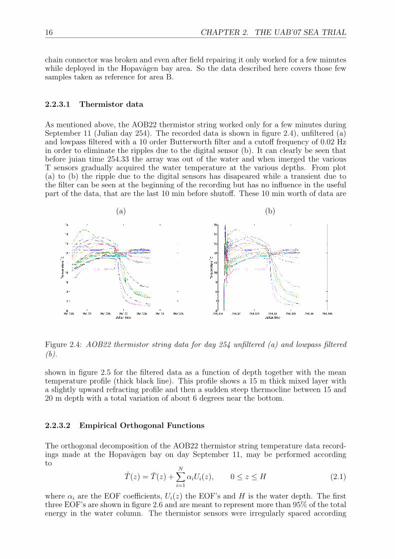
As mentioned above, the AOB22 thermistor string worked only for a few minutes duringSeptember 11 (Julian day 254). The recorded data is shown in figure 2.4), unfiltered (a)and lowpass filtered with a 10 order Butterworth filter and a cutoff frequency of 0.02 Hzin order to eliminate the ripples due to the digital sensor (b). It can clearly be seen thatbefore juian time 254.33 the array was out of the water and when imerged the variousT sensors gradually acquired the water temperature at the various depths. From plot(a) to (b) the ripple due to the digital sensors has disapeared while a transient due tothe filter can be seen at the beginning of the recording but has no influence in the usefulpart of the data, that are the last 10 min before shutoff. These 10 min worth of data are

(a) (b)

Figure 2.4: AOB22 thermistor string data for day 254 unfiltered (a) and lowpass filtered(b).

shown in figure 2.5 for the filtered data as a function of depth together with the meantemperature profile (thick black line). This profile shows a 15 m thick mixed layer witha slightly upward refracting profile and then a sudden steep thermocline between 15 and20 m depth with a total variation of about 6 degrees near the bottom.

2.2.3.2 Empirical Orthogonal Functions

The orthogonal decomposition of the AOB22 thermistor string temperature data record-ings made at the Hopavagen bay on day September 11, may be performed accordingto

T (z) = T (z) +N∑

i=1

αiUi(z), 0 ≤ z ≤ H (2.1)

where αi are the EOF coefficients, Ui(z) the EOF’s and H is the water depth. The firstthree EOF’s are shown in figure 2.6 and are meant to represent more than 95% of the totalenergy in the water column. The thermistor sensors were irregularly spaced according

2.2. GROUND TRUTH MEASUREMENTS 17

Figure 2.5: low-pass filtered AOB22 temperature profiles from thermistor string data forthe first 10 minutes of day 254; thick line is the mean temperature profile.

to the hydrophone positions of figure 2.10 and reported in table 2.1 but covering thesignificant part of the water depth. A total of 125 profiles were used for this calculation.

Figure 2.6: first three EOF’s computed from thermistor chain data during the Hopavagenbay part of the UAB07 experiment.

2.2.3.3 Sea surface and tidal corrections

The Hobo autonomous recorder was used to measure the total tidal displacement duringthe day. Figure 2.7 shows the depth and temperature recording made with the Hoborecorder located in the bottom near the pier. It can be seen that the water depth varies


between a minimum of 0.299 m up to 1,167 m with, therefore, a total variation of 0.867m with a clear period of 12,24 hours due to the tide. This curve allows for the correction

Figure 2.7: Hobo autonomous recording water depth (top) and temperature (bottom), nearthe pier to infer tidal variation in the bay.

of water depth tidal induced variations during the acoustic transmissions.

2.3 Deployment geometries in the Hopavagen Bay

Signals were transmitted from a double source array and received on the 16 hydrophoneAOB22 attached in a line between two existing moorings (see photo of figure 2.8).

Figure 2.8: AOB and source moorings at the Hopavagen Bay.

2.3.1 Acoustic source array

The acoustic source array was formed by two 916C Lubell acoustic sources arranged asshown in figure 2.9. The top buoy position was measured with an hand held GPS and

2.3. DEPLOYMENT GEOMETRIES IN THE HOPAVAGEN BAY 19

gave the following position: 63◦ 35.5862’ N, 009◦ 32.4035’ E.

Figure 2.9: sketch of the source array mooring and configuration.

2.3.2 AOB geometry: depth and range

The AOB22 was attached to an horizontal line stretched between two existing mooringsin the bay as shown in figure 2.10. The 16-hydrophone array was hand folded beforedeployment so as to comply with the reduced water depth at the array location. Amidlle array attach point was appropriately made so as to allow fixing the 8 Kg weightin order to maintain the array as much vertical as possible. Table 2.1 shows a doubleentry list of hydrophone depths according to hydrophone number or depth. Water depth

Figure 2.10: sketch of the AOB folded receiver array during the mooring at Sletvik.

at the array location was estimated to be 26 to 28 m, always subject to tidal variationsas measured by the Hobo depth sensor (see section 2.2.3.3). The AOB22 was slightlymoving within an estimated radius of a few meters. This radius is exteremely difficultto measure since its value is induced by a small movement that is within GPS accuracy,


as shown in plots of figure 2.11 for the three days when the buoy was deployed. It canbe seen that the movements from the bouy around the mooring were mostly due to GPStracking error. The black square denotes the mean position and the black circle is the onestandard deviation bound. Clearly, in this case the AOB would benefitiate from a D-GPScorrected positioning systems such as WAAS or EGNOS. The red square is the acousticmooring location so, in a mean the green line represents the underwater acoustic barrier.A GPS was positioned on top of the source mooring for a whole day and gave a mean

Hyd # Depth Hyd # Depth Depth Hyd # Depth Hyd#(m) (m) (m) (m)

1 6.6 9 7.7 3.8 10 14.6 32 10.6 10 3.8 5.7 11 15.6 73 14.6 11 5.7 6.6 1 17.6 144 18.6 12 9.7 7.7 9 18.6 45 22.6 13 13.7 9.7 12 19.5 66 19.5 14 17.6 10.6 2 20.5 167 15.6 15 21.5 11.6 8 21.5 158 11.6 16 20.5 13.7 13 22.6 5

Table 2.1: AOB hydrophone double entry depth table: by hydrophone number and byhydrophone depth.

position of 63◦ 35.5862’N 009◦ 32.4035’ E. Using this value and the AOB22 position offigure 2.11 allowed to calculate the source range in m as shown in figure 2.12.

The source range mean values and standard deviations are shown in table 2.2. As a last

Day Mean SR SR std(m) (m)

Sep.11 108 7.5Sep.12 130 3.7Sep.13 97 3.2

Table 2.2: GPS estimated source - receiver range in meter.

geometry information, during day September 13, the barrier was several times crossed bya submerged alluminium plate meant to be a target. The GPS estimated trajectory of theboat towing the target is shown in figure 2.13: GPS position relative to the barrier of (a),target depth of approximately 4.4 m (b) and source - target estimated range (c). It shouldbe taken into account that since the GPS receiver was on the boat that was towing thetarget, the target was slightly off the boat suspended from a surface buoy towed severalmeters behind the boat. In order to minimize the noise, the boat was moving using therows and the outboard engine was off. Plot of figure 2.13(c) is rather strange since itseems that the plate is at rest during long periods of time, so there might be some erroron the GPS acquisition made with a handheld PDA. In fact the crossing of the barrierwas envisioned from land taking the alignment between the source signaling surface buoyand the AOB22 and the times recording. These times are shown in table 2.3 togetherwith the direction of crossing where E - W means from the entrance to the inside of thebay and vice-versa. The crossings were made as much as possible perpendicular to thebarrier and at low rowing speed. As it can be noticed the GPS tracks (in red) of figure2.13(a) do not show the actual target movements so this data should be discarded for thepurpose of actually determining source - target range as shown in plot (c).

2.3. DEPLOYMENT GEOMETRIES IN THE HOPAVAGEN BAY 21

Figure 2.11: AOB22 GPS position during the Hopavagen bay deployments of days 11,12 and 13 of September, 2007: source position (red square), mean array poistion (blacksquare), one standard deviation on GPS position of receiving array (thick circle), meanacoustic barrier position (green line).

Direction Boat Target buoyW - E 16:06:32 16:07:32E - W NR NRW - E 16:10:59 16:12:32E - W 16:14:39 16:15:12W - E 16:17:04 16:17:36E - W 16:21:52 16:22:23W - E 16:23:50 16:24:19E - W 16:25:36 16:26:03

Table 2.3: Underwater barrier crossing: crossing direction, boat time and target buoy time(NR= crossing not recorded).


Figure 2.12: AOB22 GPS estimated source range variations along time for days 11, 12and 23 September, 2007.

Figure 2.13: Day 256, September 13, 2008: target GPS estimated position (a), sourcedepth (b) and source - target range (c).

Chapter 3

Acoustic data

Acoustic transmissions performed during the Hopavagen bay phase of UAB’07 were uniquesince in many occasions the received signals were processed and retransmitted throughthe source array (reciprocal transmissions). The experimental setup for signal controland processing is depicted in figure 3.1. The base station ensured the control of the

Figure 3.1: experimental setup for signal control and processing during the Hopavagen bayexperiment.

data acquisition on the buoy, while part of the acquired data (generally only one acousticchannel) was transmitted in real time to the TR processing computer that, after signaldetection, time-reversal and conditioning was sending the transmit signal to the sourcesignal generation computer that, itself was directly driving the source array.

23

24 CHAPTER 3. ACOUSTIC DATA

3.1 Emitted signals

The signals emitted by the source array, during the Hopavagen bay phase, were essen-tially composed by linear frequency modulated (LFM) chirps either up or down sweeps,of various durations, center frequencies and frequency bands (see table 3.1). A time -frequency sketch of the typical transmit sequence is shown in figure 3.2 where two mainphases can be seen:

1. the source initialization phase where each source is excited, one at a time, witha series of LFMs with a predetermined duration, repetition rate, center frequency,and bandwidth whose typical values are shown in table 3.1; various combinations ofthose values are possible and have been used during this phase of the experiment.

2. the retransmit phase where the array received signals are processed and thensimultaneously retransmitted in both sources with a given repetition rate and for anumber of repetitions during a certain amount of time.

Figure 3.2: Time - frequency sketch of the typical transmit sequence.

During the three days of testing there were variations of these typical cases with in-terrupted sequences, errors on the signal detection on the receiver side and then wrongretransmissions, etc... The retransmitted sequences are much more difficult to define since

Signal type LFM-up, LFM-downNumber of signals Nb 1 or 6Duration (s) Tb 0.2, 0.5 or 1Rep. rate (s) Tr 0.5, 1 or 2Time interval (s) Ti 1 or 2Center frequency (kHz) fc 5(LF), 9(MF) or 14(HF)Bandwidth (Hz) B 3000

Table 3.1: Emitted signal’s characteristics during the Hopavaagen bay phase.

they depend both on the received signals and on further processing to detect, isolate andtime-reverse the signal. In particular the “TR signal proc” computer on figure 3.1 issending commands to the AOB22 DSP in order to perform channel selection and signalpre-processing (see section 3.4.2 below).

3.2. SIGNAL GENERATOR AND AMPLIFIER 25

3.2 Signal generator and amplifier

A block schematic of the signal generation and transmission is shown in figure 3.3. Thesignal generation system used was developed at SiPLAB/CINTAL (see details in [6])and is composed of: i) one desktop computer fitted with a PCI DAC board, ii) a signalconditioning unit, iii) and audio amplifier and iv) two identical Lubell 916C sound sources.The main characteristics of the system as a whole are as follows: i) 100 kHz sampling

Figure 3.3: Signal generation system used during the Hopavagen bay phase of UAB07.

frequency, ii) 12 bits resolution DAC, iii) 1 - 16 kHz bandwidth and iv) an approximatesound pressure level (SPL) of 170 dB/µP/m on each source.

3.3 Acoustic sources

The Lubell 916C source is shown in figure 3.4(a) while its transmitt voltage response(TVR) is shown in figure 3.4(b). It can be seen that the source response is non flat inthe frequency range of interest showing a variation up to 10 dB With a maximum power

(a) (b)

Figure 3.4: Lubell 916C sound source (a) and transmitt voltage response - TVR (b).

supply voltage of approximately 14 V, gives a gain of anoter 23 dB that should be addedto the TVR curve so as to obtain the final SPL.


3.4 Received signals

3.4.1 Data format

Both the acoustic and non acoustic data received on the AOB are stored on data filesusing a proprietary format that can be read using the routine ReadLOCAPASS.m shownin appendix A. This format can be summarized as follows:

• an ASCII header: cruise title, UTC GPS date and time of first sample on file,Lat - Lon GPS position, characteristics of non-acoustic and acoustic data such assampling frequency, number of channels, sample size and total number of samples

• non-acoustic data: temperature data in binary format

• acoustic data: acoustic data in binary format

Each data file contains 24s worth of data and there is no data loss between files. Datafiles are acquired in sequence with file names reflecting julian day, hour, minutes andseconds with the extension ”.vla”. The time used in the file name is obtained from thecomputer clock so it should not be used for synchronization purposes as it is almostcertainly diferent from the GPS time in the header. The time stamp in the header ofeach file is the exact GPS - GMT time of the first acoustic sample in the fileand it can/should be used for synchronization and time of flight measurement purposes,if necessary. The sampling frequency used during UAB07 was precisely 50000 Hz (GPSclock synchronized). The Lat/Lon location written in the header is that given by theAOB GPS at the time of the first sample. A decimal degree notation was used in orderto simplify its usage for calculation and plotting purposes (inside Matlab, for example).

3.4.2 Channel selection and summation

During the first two days of this phase a real time procedure was developed, setup andtested to perform channel selection and summation on the AOB receiver side in order toavoid offline processing and to speed-up wireless communications. The basic idea was toperform channel summation on the AOB DSP during signal acquisition and transmit theresult to the “TR signal proc” computer for processing and retransmission. The tasksperformed by the DSP were very simple: 1) select channels according to a code given bythe user in a command file, 2) accumulate the 16 bit words in a 32 bit buffer, 3) shiftthe 32 bit buffer 4 times to the right, which is equivalent to a division by 16, 4) writethe resulting 16 LSB bits to channel 4 (damaged during phase 1 and therefore not usedanyhow).

Channel selection was made by using a coding scheme where the N selected channelswhere designated by a single code given by Code =

∑Ni=1 2Channel numberi−1. Unfortunately

there was an error during the decoding which resulted in the following channel selections:

Code Selected channels---- -------------------516 5,6,7,8,13,14,15,16532 5,6,7,8,13,14,15,16

3.4. RECEIVED SIGNALS 27

567 1,2,5,6,7,8,9,10,12,13,14,15,1665527 1,2,5,6,7,8,9,10,12,13,14,15,16

3.4.3 The 4 by 4 repetition problem

As explained above during this phase in the Hopavagen bay, the received acoustic signalswere acquired and stored on the AOB. In order to fullfil with the requirement for on the flyprocessing and retransmit for acoustic barrier implementation, the acquisition programwas modified for post channel selection, summation and writing on top of channel 4.During the writing of this report it was found that due to a, at this time, unknown reason,the acquisition process failed to switch channel at the input of the AD converter whichresults in that all data files, instead of the 16 channels, contain just 4 times 4 channels.Therefore channel 1, is repeated in channels 2, 3 (channel 4 was used for saving all channelsaverage) channel 5 is repeated in channels 6 to 8, channel 9 is repeated in channels 10 to 12and finally channel 13 is repeated in channels 14 to 16. This is more clearly understoodby observing figure 3.5 that shows the estimated channel impulse responses by pulsecompressing the received with the emitted signal for each array channel from 1 to 16.Channel depths are shown on each line and follow the array folding pattern of table 2.1.As it can clearly be seen signals are equal within each block of four, except for channel

Figure 3.5: Day 254 14:12 UTC: pulse compression of all channels with LFM upsweep0.2 s duration in the band LF band: 3500 - 6500 Hz.

4 that has the mean of all channels. At this point it seems that the only channels thatcan be used for the processing are those which impulse responses are shown in figure 3.6.Interestingly, this figure shows a relatively depth constant 4-arrival pattern for the upperhydrophones and a time shifted pattern with four well separated arrivals for the deeper(22 m) receiver. In the sequel we will focus only on channels 1, 5, 9 and 13.


Figure 3.6: Day 254 14:12 UTC: pulse compression of channels 1, 5, 9 and 13 at respectivedepths of 6.6, 22.6, 7.7 and 13.7 meter [LF upsweep 0.2 s duration in the LF band: 3500-6500 Hz].

3.4.4 Day 254 (September 11, 2007)

This first day was mostly spent on testing the source array and then the receiving array.The AOB22 was deployed at 07:55 GMT and acquisition started at 08:07 GMT. A shortlog of the received signal sequences is given in table 3.2. The first test signals were

Time Event fc Bw Dt(GMT) (kHz) (kHz) (s)08:07 start ACQ09:35 start coms (OFDM) 10 4/8 109:41 end coms (OFDM)11:37 start up/down LFM 5 3 0.514:10 end up/down LFM14:12 start up/down LFM 5 3 0.2

(several changes)17:29 end ACQ

Table 3.2: Signals’ sequences log during day 254 (11 September 2007) in the Hopavagenbay.

transmitted at 09:35 using one of the Lubell 911C sound sources ending at 09:41. Thesewere OFDM communication signals with a center frequency of 10 kHz interleaved withup and down LFM sweeps covering the whole frequency band as shown on figure 3.7 onhydrophone 1 at 6.6 m depth (see a complete description on the companion report PartB for the Trondheim site data set).

At 11:37 started a series of up and down LFM sweeps of 3 kHz bandwidth centered


Figure 3.7: Day 254: OFDM communication signals for source testing as received onhydrophone 1 (6.6 m depth).

on 5 kHz and with 0.5 s duration and 0.5 s interleave. Approximately 80 s after startingsignal transmission a series of harmonics appeared above 7 kHz and more clearly above10.5 kHz, in coincidence with the transmitted pulses, and for which, up to now, there isno convincent explanation. These are shown in figure 3.8, where second order harmonicsare starting at 7 kHz and third order harmonics are starting at 10.5 kHz, the later muchmore clearly. The harmonics have the same duration as the original signal but coverfrequency bands that are two and three times larger, 6 and 9 kHz respectively1. Themultipath is clearly longer than the signal interleaving resulting in a superposition ofthe impulse responses of the various pulses. Strangely enough a multipath can be seenalso on the third harmonic. At 14:12 h the transmission resumed with the same centerfrequency, bandwidth and repetition rate but with shorter duration of only 200 ms in orderto have a larger interval for the channel multipath. As in the previous run, the harmonicsappeared approximately 80 s after the transmission started. The rest of Julian day 254was spent on transmitting up and down sweeps in the 5 kHz band. The pulse compressionof that sequence for the 0.2 second duration upsweep averaged over each 24 second file isshown in figure 3.9(a) for hydrophone 1 at 6.6 m depth. This result was obtained witha pre bandpass filter of 4 kHz centered in 5 kHz so as to eliminate the harmonics. Thealignement of the mean replicas has shown an extremely small synchronization error witha standard variation of 8 µs over more than 2 hours of data which is a proof of stabilityof the channel and the source - array geometry. A detailed view of the mean arrivalpattern is shown in figure 3.9(b), where a main arrival and 3 multipaths can be clearlydistinguished.

1this is not very clear for the second order that shows a large attenuation but is clear for the thirdorder that, however suffers the cutoff of the antialiasing filter at 16 kHz.


Figure 3.8: Day 254 hydrophone 1 (6.6 m depth): up - down sweeps in the lower 5 kHzband and corresponding harmonics.

(a) (b)

Figure 3.9: Day 254, hydrophone 1 (6.6 m depth): arrival pattern for the 3 kHz band upsweep along time (a) and mean arrival pattern (b).

3.4.5 Day 255 (September 12, 2007)

Most of this day was spent on adjusting the signal detection on the receiver side for re-transmission on the source side. Also some changes were done on the acquisition programfor allowing the selection of the channels to be summed into channel 4. The sequence ofevents is shown in table 3.3. At 10:30 started a long sequence of 0.5 s duration upsweepsin the 7.5 - 10.5 kHz that lasted for approximately 80 min. The pulse compression of thatsequence is shown in figure 3.10 for channel 5 at 22.6 m depth: the channel variabilityalong time (a) and the mean arrival pattern (b). The correlation peak variability couldbe measured of the order of 0.034 s with a standard variation of 0.238 ms. There arefour distinct paths possibly associated with the bottom reflected, direct, bottom - surface


Time Event fc Bw Dt(GMT) (kHz) (kHz) (s)07:19 start ACQ08:17 start LFMs up 5 3 0.509:07 LFMs by packs of 12 5 310:10 LFMs by packs of 12 10 3 0.5

alternate LF and MF12:46 source probes and

TR replicas14:10 end up/down LFM14:12 start up/down LFM 5 3 0.2

(several changes)17:29 end ACQ

Table 3.3: Signals’ sequence log during day 255 (12 September 2007) in the Hopavagenbay.

(a) (b)

Figure 3.10: Day 255 hydrophone 5 at 22.6 m depth, 0.5 s LFM sweeps in the 7.5 - 10.5kHz band, start time 10:31 UTC: time variability (a) and mean arrival pattern (b).

reflected and surface - bottom reflected. This is mainly due to the strongly downwardbathymetric propagation profile.

3.4.6 Day 256 (September 13, 2007)

This last day was devoted to an attempt of implementing the actual acoustic barrierwhile simulating the target with a submerged square alluminium plate of approximatedimensions of 1,2 × 1.2 m towed by a small rowing boat in between the source and theacoustic array (the barrier). Unfortunately this day testing was also shortened due toa faulting connection on the battery charge during the night that left the battery stilldischarged in the morning. The battery was then put on charge in the morning andthe AOB could be deployed around 12:30. The data acquisition was switched on at13:05 GMT (see table 3.4). After 14:51 the probe source signals were followed by longsuccessive transmissions of time-reversed replicas so as to reflect in the barrier crossingtarget (see table 2.3 for a log of target barrier crossings). Various center frequencies


were tested during the several target crossings. The list below shows the output of a log

Time Event fc Bw Dt(GMT) (kHz) (kHz) (s)13:05 start ACQ13:06 LFMs up, TR replicas 14.5 3 0.513:17 LFMs up, TR replicas 5 313:32 LFMs up, TR replicas 10 3 0.513:40 stop ACQ13:41 restart ACQ13:51 LFMs up, TR replicas 10 3 0.514:02 LFMs up, TR replicas 5 3 0.514:12 LFMs up, TR replicas 14.5 3 0.514:51 LFMs up, long TR 14.5 3 0.5

alternate LF,MF,HFlong TR transmission

17:37 end ACQ

Table 3.4: Signals’ sequences log during day 256 (13 September 2007) in the Hopavagenbay.

file containing all the channel sum settings during day 256. This log was filtered fromthe complete AOB22 log file screenlog.0 written during the data acquisition. In thatlog, an indication of channel codes 516, 532, etc, means that the corresponding channelnumbers where selected and summed into channel 4. The relation between the codeand the channel number was already explained in section 3.4.2. Unfortunately, due to aprogramming glitch, the settings were those given in the table below and ended in caseswhere different codes gave the same channel numbers and not those expected.

UTC Channel Channelcodes numbers

12:59:08 0 013:07:40 516 5 6 7 8 13 14 15 1613:13:21 0 013:17:45 516 5 6 7 8 13 14 15 1613:20:33 532 5 6 7 8 13 14 15 1613:23:45 567 1 2 3 5 6 7 8 9 10 11 12 13 14 15 1613:26:33 65527 1 2 3 5 6 7 8 9 10 11 12 13 14 15 1613:32:33 516 5 6 7 8 13 14 15 1613:35:45 532 5 6 7 8 13 14 15 1613:38:33 567 1 2 3 5 6 7 8 9 10 11 12 13 14 15 1613:41:23 0 013:51:47 516 5 6 7 8 13 14 15 1613:54:59 532 5 6 7 8 13 14 15 1613:57:23 567 1 2 3 5 6 7 8 9 10 11 12 13 14 15 1613:59:23 65527 1 2 3 5 6 7 8 9 10 11 12 13 14 15 1614:02:35 516 5 6 7 8 13 14 15 1614:04:59 532 5 6 7 8 13 14 15 1614:06:59 567 1 2 3 5 6 7 8 9 10 11 12 13 14 15 1614:08:59 65527 1 2 3 5 6 7 8 9 10 11 12 13 14 15 1614:12:35 516 5 6 7 8 13 14 15 16

3.5. SIGNAL DETECTION 33

14:14:59 532 5 6 7 8 13 14 15 1614:16:59 567 1 2 3 5 6 7 8 9 10 11 12 13 14 15 1614:19:23 65527 1 2 3 5 6 7 8 9 10 11 12 13 14 15 1616:30:01 0 016:32:01 65527 1 2 3 5 6 7 8 9 10 11 12 13 14 15 16

This table of channel summation setups clearly shows that during the crossing of thebarrier with the simulated target there was one single configuration using all the channelsbut channel 4: time interval between 16:06 and 16:30. This will be our primary target foranalysis. Taking into account the problem of channel duplication this table also impliesthat :

• in positions 516 and 532, channel 4 contains 4 × channel 5 + 4× channel 13, dividedby a factor of 16 (add in 32 bits and drop of the 4 least significant bits)

• in positions 567 and 65527, channel 4 contains 3× channel 1 + 4× channel 5 + 4×channel 9 + 4× channel 13, divided by a factor of 16 (add in 32 bits and drop ofthe 4 least significant bits)

In order to illustrate the data collected during day 256, figure 3.11 shows the time-compressed estimated channel impulse responses for the 4 active channels in the threefrequency bands. The most strinking feature is the appearence of a fast sediment orclose to sediment wave in the bottom hydrophone that becomes more apparent as thefrequency increases. This is probably due to the strong downslope propagation effectwhere the water wave and the sediment interaction reflection are very close in both timeand space.

3.5 Signal detection

One of the scopes of this phase of the UAB07 experiment was to attempt to detect atarget crossing the barrier. There are a number of possible sub-optimal implementationsof the theoretical detector, among which one is obtained by performing the summationof the time-reversal (TR) focus after reciprocal TR for all or some of the array channels.The so-called single implementation is therefore obtained as follows:

1. transmitt a given broadband signal from each of the sound sources, one source at atime.

2. detect the received signals and sum the selected channels on a single stream; repeatthat for each source.

3. retransmitt the time-reversed versions of the channel sum streams simultaneouslyfrom each respective source.

4. collect the received signals and sum the selected channels (focus) after correlatingwith the time reversed version of the initially transmitted broadband signal; peekthe maximum of the time correlations (or the maximum of the envelop if in baseband).


(a) (b)

(c)

Figure 3.11: Day 256 impulse responses between sound source at 3 m depth (S1) and eachhydrophone for frequency bands : 3500 - 6500 Hz (a), 7500 - 10500 Hz (b) and 12000 -15500 Hz (c).

5. build the detector by comparing the result obtained from one snapshot to anotherplus a given threshold, to be adjusted according to the desired false alarm rate andexisting SNR.

The word simultaneously was highlighted because it is important to keep coherencefrom one sound source to another since sound sources are positioned at different depths,and eventually at slightly different ranges in the case of tilted arrays, thus covering dis-tinct portions of the water column. In order to obtain synchronized focus after reciprocalTR, and thus an effective time summation of the energies over the array, each sourcesequence should not be detected separately from the other. Failling of doing so, wouldresult in retransmitting asynchronous sequences on each source that will, most certainly,arrive out of phase at the array since the inter - source information is lost during the de-tection / synchronization process between transmissions. Unfortunately this was exactlywhat happened during the experiment: the sequences from the two sources wereseparately detected and synchronized before retransmission. The result of thisprocedure can be seen in figure 3.12: the time-frequency plot on the left shows two seriesof upsweeps in the LF band for initialization of source 1 and 2, respectively, and then thereciprocal receptions as received on channel 4 at time 13:20:57 UTC, where channels 5 to8 and 13 to 16 were selected for summation. This process can be equated as follows: letus assume x(t; k, l) as given by

x(t; k, l) = h(t; k, l) ∗ s(t) (3.1)

3.5. SIGNAL DETECTION 35

Figure 3.12: Day 256 hydrophone 4 at 13:27 UTC as a summation of several channelsaccording to the tabel above: time - frequency (left) and time compressed time series (left),source 1 (a) and source 2 (b).

to be the noise free signal received on sensor k due to source l at time t response to theemitted signal s(t), assumed the same for all sound sources. In our experiment channel 4contains the sum of a selection of received signals, thus

x(t; l) =K∑

k=1

x(t; k, l)

=K∑

k=1

h(t; k, l) ∗ s(t) (3.2)

In this case the reciprocal received signal (always in the noise free case) is then given by

p(t; k) =L∑

l=1

h(t; k, l) ∗ x(−t; l)

=L∑

l=1

h(t; k, l) ∗K∑

k=1

h(−t; k, l) ∗ s(−t) (3.3)

where L is the total number of sources, in our case L = 2. The received signal on sensork is therefore the sum of four terms

p(t; k) = h(t; k, 1) ∗ h(−t; k, 1) ∗ s(−t) +L∑

l 6=k

h(t; k, 1) ∗ h(−t; k, 1) ∗ s(−t) +

h(t; k, 2) ∗ h(−t−∆; k, 2) ∗ s(−t−∆) +L∑

l 6=k1

h(t; k, 2) ∗

h(−t−∆; k, 2) ∗ s(−t−∆) (3.4)

where the delay ∆ represents the artificial delay introduced by the synchronisation be-tween the two source signals. This simple delay makes that the focus for source 1 and 2are not added at the h(t) ∗ h(−t) correlation peak. The other terms are interference orcross terms. Since the number of sources L is low the rejection ratio between the focusand the cross terms is also low but still, autocorrelations should provide a higher peakthan cross-correlations.


The effect of this delay can better be seen in the correlation of the received signalswith the HF downsweep during day 256 that produces the result shown in figure 3.13.There is a clear severe time spread incompatible with what would be expected as a focusin time of the reciprocal transmissions. In fact there are two main peaks surrounded bysidelobes, indicating that this signal could be formed by the sum of two or more focuswithin a time interval or approximately 1.5 ms. Since it is very unlikely that the source -array geometric structure or the environment would change so dramatically so as to causethis delay, therefore the most plausible explanation is the lack of coherent detection ofthe two source signals prior to reciprocal transmission resulting in an artificially alignedreciprocal transmission. The horizontal lines represent the moments when the simulated

(a) (b)

(c) (d)

Figure 3.13: Day 256 correlations with HF downsweep pulse starting at 16:01 UTC forchannels: 1 at 6.6 m depth (a), 9 at 7.7 m depth (b), 13 at 13.7 m depth (c) and 5 at22.6 m depth (d). Signal transmission was interrupted and re-initialized at 16:18 UTC.Horizontal lines mark the target crossings of the virtual barrier according to measuredtime of table 2.3.

target crossed the barrier formed by the source array and the receiving array as measuredby the GPS and line of sight during the experiment (see list of table 2.3). At first glancethere is no particular correlation between the time compressed reciprocal received signaland the target crossings.

Chapter 4

Conclusions and future analysis

The UAB project aims at studying, developing and testing acoustic methods for protectingcritical infrastructures. The UAB07 experiment served at: i) testing high frequency signalsoff the busy port of Trondheim, Norway, and ii) proving the acoustic barrier concept inan acoustically quiet and environmentally stable location in the Hopavagen bay, 200 kmfrom Trondheim, Norway. This report concentrates on the experiment carried out atthe Hopavagen bay, from September 9 to 13. The location turned out to be ideal fordeploying the source and receiving array and its operation from land. The time spentin equipment installation and extensive debugging of hardware and software resulted inpractice in only half day of actual acoustic barrier data. The results obtained confirmedan extremely stable environment with reproductible conditions in short (minutes) andlong (hours) time frames. Parallel results obtained with simulations and not shown inthis report showed that the limited environmental data gathered during the sea trialwas sufficient to run computer models for determining signal propagation conditions thatcan explain the transmission patterns found during the experiment. However, due totwo major drawbacks it appears extremely difficult to achieve target detections with theobserved data sets. These drawbacks are:

• the limited number of receiving channels (4) due to the replication of every forthchannel in the following three.

• the loss of synchronization between the two source received signals before reciprocalretransmissions.

As recommendations for future experiments and apart from the obvious correctionof the above mentioned drawbacks, future experiments involving acoustic barriers shouldaccount for: i) saving reciprocal signals as transmitted from source array, ii) high precisionGPS for surface buoy location through time, iii) real time correlation of received signalswith time-reversed replica of the emitted signal beofre channel summation and iv) ifpossible, increase the number of sources in the active array.

37

Bibliography

[1] C.R. Bates and E.J. Whitehead. Echoplus measurements in hopavagen bay, norway.Sea-Technology, 42(6):34–43, June 2001.

[2] S.M. Jesus. Active acoustic time-reversal for underwater acoustic barriers. In 153thMeeting of the Acoustical Society of America, volume 121 - 5 Pt.2, page 3204, SaltLake City, USA, May 2007.

[3] F. Zabel, C. Martins, Jesus S.M., and Silva A. Tra - transmit receive array (projectplan). Internal Report Rep. 05/06, SiPLAB/CINTAL, Universidade do Algarve, Faro,Portugal, September 2006.

[4] F. Zabel, C. Martins, Jesus S.M., and Silva A. Tra - transmit receive array (projectplan - version 2). Internal Report Rep. 02/07, SiPLAB/CINTAL, Universidade doAlgarve, Faro, Portugal, March 2007.

[5] F. Zabel and C. Martins. Analog 16-hydrophone vertical line array for the acoustic -oceanographic buoy - aob. Internal Report Rep. 03/06, SiPLAB/CINTAL, Universi-dade do Algarve, Faro, Portugal, August 2006.

[6] C. Martins. Uab07 transmission system technical specifications. Internal report,SiPLAB-CINTAL, University of Algarve, 2008.

38

Appendix A

Data reading routine:readlocapassdata.m

function [data, Fs, NoSs, TITLE, TIMEPOS]=ReadLOCAPASSData(filename,DataType);%% Reads a Data File from the LOCAPASS DAQ System%% [data, fs, NoSs, TITLE, TIMEPOS]=ReadData(file,flag)%% Where:% data: is a matrix [ NoChannels * Total No Samples ]% fs: sampling frequency% NoSs: Number of Channels% TITLE: Description of the experiment% TIMEPOS: Time/Position information of the data in the file%% file: name of file to be read, empty variable will allow% theselection of the file to read, recognized extensions:% * ".acust" - Acoustic Data% * ".tilt1"/".tilt2" -Array Inclination Data% * ".pr1"/".pr2" -Array Depth Data% * ".temp" - Temperature Data% * ".dummy" - Battery Voltage Data% flag: if greater than 0, return values of data will be converted% to its usable System Units ( volts, degrees of inclination,% meters, etc )%if ( nargin < 2 )

error(’Two parameter are required\n Sintax:ReadLOCAPASSData(filename,...DataType);\n DataType must be"acoustic" or "nonaccoustic"’);

end

disp([’Trying to open: ’ filename ’ !!!’]);fid = fopen(filename,’r’);if (fid==-1)

error([’File:’ filename ’could not be open!!’]);

39

40 APPENDIX A. DATA READING ROUTINE: READLOCAPASSDATA.M

enddisp(’File Openned!!’);

TITLE = fgetl(fid);teststr(TITLE);

TIMEPOS = fgetl(fid);teststr(TIMEPOS);

NonAcdatainfo = fgetl(fid);%NonAcdatainfo= ’nonACOUSTIC Fs:0 NoSens:0 SampSz:0 TotS:0’teststr(NonAcdatainfo);%fgetl(fid);

Acdatainfo = fgetl(fid);%Acdatainfo = ’ACOUSTIC Fs:63999 NoSens:08 SampSz:32 TotS:31457280’teststr(Acdatainfo);%fgetl(fid);

switch DataTypecase ’timeposition’,

data = [];count = 0;Fs = str2num(NonAcdatainfo(16:20)); % Sampling frequencyNoSs = str2num(NonAcdatainfo(29:30)); % No of ChannelsSpSz = str2num(NonAcdatainfo(39:40)); % No of Bits per SamplesToSp = str2num(NonAcdatainfo(47:54)); % Total Number of Samples

case ’nonacoustic’Fs = str2num(NonAcdatainfo(16:20)); % Sampling frequencyNoSs = str2num(NonAcdatainfo(29:30)); % No of ChannelsSpSz = str2num(NonAcdatainfo(39:40)); % No of Bits per SamplesToSp = str2num(NonAcdatainfo(47:54)); % Total Number of Samplestestinfo(Fs); testinfo(NoSs); testinfo(SpSz); testinfo(ToSp);if NoSs > 0

[data count]=fread(fid,[NoSs ToSp/NoSs],[’int’ num2str(SpSz)]);else

data = [];count = 0;

endcase ’acoustic’

NoSs = str2num(NonAcdatainfo(29:30)); % No of ChannelsSpSz = str2num(NonAcdatainfo(39:40)); % No of Bits per SamplesToSp = str2num(NonAcdatainfo(47:54)); % Total Number of Samplesif NoSs > 0

[data count]=fread(fid,[NoSs ToSp/NoSs],...[’int’ num2str(SpSz)]); %skip NonAc data

end

Fs = str2num(Acdatainfo(16:20)); % Sampling frequencyNoSs = str2num(Acdatainfo(29:30)); % No of ChannelsSpSz = str2num(Acdatainfo(39:40)); % No of Bits per SamplesToSp = str2num(Acdatainfo(47:54)); % Total Number of Samplestestinfo(Fs); testinfo(NoSs); testinfo(SpSz); testinfo(ToSp);

41

[data count]=fread(fid,[NoSs ToSp/NoSs],[’int’ num2str(SpSz)]);otherwise,

fclose(fid);error(’Wrong data type!’)

end

disp(’Data Read!’)fclose(fid);disp(’File Closed..’)

if count < ToSpdisp(’Not a Full File!’);

end

return

%*****************************************************************% ********** Auxiliary Functions*******************************%*****************************************************************

function teststr(strarr)if ~ischar(strarr)

error(’Not a Valid DATA file!!’);endreturn

function testinfo(valuearr)if isempty(valuearr)

error(’Not a Valid DATA file!!’);endreturn

function out=gettype(strarr)

found=findstr(strarr,’.’);if isempty(found)

error(’No Filename extension!!!’)else

out=strarr((found(end)+1):end);end

underwater acoustic barriers experiment uab’07 part a: the

Documents