unemployment and potential output in the 1980s · unemployment and potential output in the 1980s...

ROBERT J. GORDON Northwestern University

Unemployment and Potential Output in the 1980s

THE TWO most outstanding features to date of the 1983-84 economic expansion are the unusually rapid decline in unemployment and the continuing deceleration of inflation. The 3.1 percentage point decline in the civilian unemployment rate in the first seven quarters of the recovery (from 10.6 percent in 1982:4 to 7.5 percent in 1984:3) was greater than in any postwar recovery since the Korean War. The inflation rate as measured by the fixed-weight deflator declined from a peak of 11.3 percent in 1980:4 to just 3.8 percent in 1984:3.

The sharp decline in unemployment and the associated creation of millions of new jobs, while creating good news for jobseekers and incumbent politicians, raise two serious questions for economic analysts and policymakers. First, is the extent of the decline in the unemployment rate consistent with the historical relationship between unemployment and output, or is there some additional, unexplained component of the recent unemployment performance? Second, does the rapid drop in unemployment have as its counterpart an unusually poor performance of productivity growth? If so, this would have important implications for competing hypotheses that have attempted to explain the post-1973 slowdown of productivity growth and in addition might imply that the underlying growth rate of potential output is slower than has generally been assumed.

The term "potential real GNP" designates the level of real gross national product that the economy could produce at a given time if it were operating at its hypothetical "natural" unemployment rate that would, in the absence of supply shocks, be compatible with a nonaccel-

537

538 Brookings Papers on Economic Activity, 2:1984

erating rate of inflation. 1 If we define the "GNP gap" as the percentage difference between actual and potential real GNP, and if we define the "unemployment gap" as the difference in percentage points between the actual and natural unemployment rates, then one indirect method for estimating the level of potential GNP is to use historical data to estimate an Okun's law coefficient, which links the two gaps. A rapid decline in the unemployment rate implies a rapid decline in the unemployment gap and, using the historical coefficient, in the GNP gap. Since the growth of actual real GNP is known, use of the historical Okun's law relationship thus provides evidence on how fast potential real GNP has been growing.

This paper analyzes why the unemployment rate fell as fast as it did in the recovery and provides new estimates of the level and growth of potential real GNP. The growth rate of potential real GNP, in turn, is decomposed into the growth rates of population, labor force participation, hours per person, and productivity per hour, thus allowing a verdict on whether, after adjustment for cyclical effects, the much-discussed slowdown of productivity growth after 1973 was intensified or alleviated after 1979. To anticipate, it appears that the slow rate of productivity growth experienced in 1974-79 has not changed appreciably since then.

The point of departure for the analysis is an identity that links real GNP with the unemployment rate and other variables, including productivity, hours, and the labor force participation rate. After a brief initial inspection of the data, a statistical relationship is estimated between the detrended level of each component of this identity and, as a single explanatory variable, detrended real GNP. The estimated equation relating the detrended employment rate to detrended real GNP is a historical Okun's law relation that can be used to determine the most plausible growth rate since 1979 for the unobservable potential real GNP.

The estimated equations for the other components of the identity are

1. Although in other writing I have preferred the term "natural real GNP," here I defer to the "potential real GNP" usage that is customary in BPEA and in government publications. There does not seem to be any consistent official terminology for the corresponding unemployment rate.

Robert J. Gordon 539

then used to decompose the post-1979 growth of potential real GNP into cyclically adjusted trend growth rates in productivity, hours, labor force participation, and so on. The end result of the paper is a consistent decomposition of the observed growth of real GNP and each component of the GNP identity between a cyclically sensitive component and a cyclically adjusted "potential" trend component.

The Cyclical Behavior of Output and Unemployment

OKUN S LAW AND THE OUTPUT IDENTITY

Okun's law postulates a regular relationship between the GNP gap and the unemployment gap. This relationship has remained popular in macroeconomic analysis both because it has been sufficiently stable and reliable in the past two decades to deserve being labeled a law and also because it short-circuits the rather complex identity that links output and unemployment.2 A simple version of this identity can be written as in one of my earlier papers,3 in which real GNP, Q, is decomposed into the employment rate, EIL; hours per employee, H; labor productivity, QIEH; the labor force participation rate, LIN; and the population, N.4

(1) Q _ ~~~E Q L H N. (1) Q=ffEHN .

The typical estimate of 2.5 to 3.0 for the Okun's law coefficient relating cyclical fluctuations in output to those in the employment or unemployment rate implies, according to identity 1, that more than half of the

2. For the original statement of Okun's law, see Arthur M. Okun, "Potential GNP: Its Measurement and Significance," in American Statistical Association, Proceedings of the Business and Economic Statistics Section 1962, pp. 98-104, reprinted in Okun, The Political Economy of Prosperity (Brookings, 1970), pp. 132-45.

3. Robert J. Gordon, "The Welfare Cost of Higher Unemployment," BPEA, 1:1973, pp. 133-95.

4. The employment rate, EIL, is simply unity minus the unemployment rate, that is, (1 - UIL).


cyclical fluctuations in output have their counterpart in cyclical movements of productivity, participation, and hours per employee.'

While identity 1 is an adequate formulation for theoretical analysis, it is incomplete for a real-world data investigation because the conven- tional measures of employment, participation, and population cover the entire civilian population (aged 16 and over), while the productivity and hours components cover the nonfarm private business sector, which is smaller. Further, the data source for civilian employment (households, in the current population survey) differs from the data source for nonfarm business employment (the establishment survey). These complications require that identity 1 be expanded as follows:

(2) - EQB

-L HBN2QE (2) Q-LEBHBN QB E'

where the variables with the B superscripts are those for the nonfarm business sector and the variables without superscripts are those for the total economy or civilian labor force.6 Identity 2 differs from identity 1 in the final two terms, which can be described as mix-effect terms and which change whenever there is a change in the ratio of total output per civilian employee, QIE, to the same ratio in the nonfarm private sector, QBIEB. Among the factors contributing to the mix-effect terms are changes in the government and farm shares of output, differential growth in government, farm, and nonfarm productivity, and discrepancies between the household and establishment employment surveys.

Identity 2 can be simplified by labeling the ratios with a single letter; with R for the employment rate, V for productivity, F for the participation rate, MQ for the output-mix effect, and ME for the employment-mix effect, it becomes

(3) Q=R VFHNMQ ME,

5. Since population, N, includes only those aged 16 and over, it is clearly unaffected by the business cycle except to the (presumably minor) extent that recessions raise the death rate by increasing the incidence of stress, mental illness, malnutrition, and suicides.

6. The expanded identity is the same (other than different notation) as equation 3 in Peter K. Clark, "Okun's Law and Potential GNP," Working Paper (Board of Governors of the Federal Reserve System, June 1983). Clark's equation is also used in modified form in Douglas M. Woodham, "Potential Output Growth and the Long-term Inflation Outlook, " Federal Reserve Bank of New York Quarterly Review, vol. 9 (Summer 1984), pp. 16-23.


where for convenience the B superscript on the hours term is dropped. The equivalent identity for components of the growth rate of real GNP is

(4) q-r + v + f + h + n + mQ + mE,

where each lowercase letter represents the annual percentage growth rate of the levels expressed as corresponding uppercase terms in identity 3.

Another form of the identity that is useful for statistical analysis expresses the relationship in terms of the natural logs of the ratios of each component to its own trend. With asterisks to designate trend variables and a circumflex to denote the natural log of each ratio of an actual value to its trend [for example, I = ln (QI Q*)], identity 3 becomes

(5) Q = R + V + F + H + N + MQ + ME

This states that deviations from trend in the employment rate, R, productivity, V, and the other components must sum to the deviation from trend of real GNP, Q, which in turn is the GNP gap or, in language I sometimes use, the output ratio.

Okun's law states that the unemployment gap is a constant fraction, k, of the GNP gap. Using the terms defined in equation 5, Okun's law can be written as the statement that the employment ratio, R, is a constant fraction, k, of the output ratio, Q:

A (6) k R

Q

This, in turn, implies that 1 - k must be equal to the sum of the remaining detrended ratios to the output ratio:

(7) 1 - k = V + F + H + N + MQ + ME (7) l -k=V -+ + + Q

A byproduct of the statistical research reported below is a decomposition showing the ratio to Q of each term in the numerator of equation 7 in the typical postwar business cycle.


COMPONENTS OF THE IDENTITY IN SEVEN

POSTWAR RECOVERIES

The first step in our analysis of the data takes the form of table 1, a simple display of the growth-rate version of identity 4. This version decomposes the observed growth rate of real GNP for the first seven quarters of each postwar recovery among the seven terms in the identity; the aborted recovery of 1980-81 is excluded, because it did not last for seven quarters. Each figure listed is an annual growth rate, so that the actual change over the seven quarters in each case is seven-fourths of the rate shown. In the 1983-84 recovery, for instance, the employment rate grew in the first seven quarters by a total of seven-fourths of 1.97, or 3.45 percentage points.7 Table 1 confirms that this was by far the fastest growth in the employment rate of any post-Korean War recovery and almost matched the record of the ebullient 1950-51 Korean War expansion, in which output grew much faster. The 1983-84 increase in the employment rate was more than six times faster than in 1975-76, the most recent comparable recovery.

On a purely arithmetical basis, most of the faster employment growth in 1983-84 compared with 1975-76 can be attributed to faster growth of output:

1975-76 1983-84

Output 4.94 6.24 Other components - 4.64 - 4.27 Difference:

employment rate 0.30 1.97

But this arrangement of the numbers is misleading, because it ignores Okun's law. Of the 1.30 extra points of output growth in 1983-84 compared with 1975-76, Okun's law states that only roughly one-third should have taken the form of growth in the employment rate. By this reckoning, employment rate growth in 1983-84 should have been the 1975-76 rate (0.30) plus one-third of the extra output growth (0.33 times 1.30), or 0.73 points instead of the 1.97 points actually observed. From

7. The employment rate rose by 3.5 points while the unemployment rate, as stated above, fell by 3.1 points. This discrepancy occurs because the 1982:4 base for calculating the growth rate of the employment rate is 0.894, not unity.


Table 1. First Seven Quarters of Postwar Recoveries: Growth Rates of Real GNP and Components of Identitya Percent at annual rates

Employ- Output Partici- Employ- Real ment per pation Average Popula- Output ment GNP, rate,b hour,c rate,d hours,e tion,' Mix,g mix,h

Period q r v f h n mQ mE

1949:4-1951:3 10.27 2.27 4.83 -0.15 0.39 0.06 0.53 2.34 1954:2-1956:1 5.29 1.05 2.50 1.07 0.43 1.21 -1.04 0.07 1958:2-1960:1 5.78 1.34 3.04 -0.71 0.51 1.57 - 1.30 1.33 1961:1-1962:4 5.19 0.77 4.15 - 1.04 0.14 1.33 -0.40 0.24 1970:4-1972:3 5.45 0.12 4.11 0.05 -0.01 2.53 - 0.95 -0.40 1975:1-1976:4 4.94 0.30 3.29 0.52 -0.03 1.93 -0.86 -0.21 1982:4-1984:3 6.24 1.97 3.34 0.31 0.86 1.16 - 2.00 0.60

Source: Computation of text's identity 4. Real GNP, U.S. Bureau of Economic Analysis. All other data, U.S. Bureau of Labor Statistics.

a. Growth rates computed as difference in logs. The 1980-81 recovery is excluded, because it did not last for seven quarters. The second through eighth columns add to the first column, net of rounding error.

b. Civilian. c. Nonfarm business sector. d. Civilian labor force. e. Nonfarm business sector, hours of all persons divided by employment. f. Civilian population aged 16 and over. g. Real GNP divided by nonfarm business real GNP. h. Nonfarm business employment, from establishment data, divided by civilian employment, from household

survey.

this perspective it seems understandable that most forecasters have been surprised, if not startled, at the pace of the increase in the employment rate and the corresponding decline in the unemployment rate during the 1983-84 recovery.

However, we should not make too much of the raw numbers displayed in table 1. The 1983-84 recovery has differed from those in the past, but we expect recoveries to differ in the relative growth rates of the components of the identity. First, the growth rates in the table are not detrended, but underlying trends in the growth of productivity, hours, and the other terms change from time to time. Second, the components of the identity adjust to changes in output with varying lag patterns and would tend to behave differently in a recovery that begins slowly and then accelerates (like 1971-72) than they would in a recovery that begins rapidly and then decelerates (like 1983-84). Thus in order to determine whether the behavior of unemployment in the 1983-84 expansion has been unusual, there is no alternative to the econometric estimation of historical relationships that takes account of lagged adjustment and shifts in underlying trends.


Regression Equations for Components-of-Output Identity

REINTERPRETING "SURPRISES AS REGRESSION RESIDUALS

Was the 1983-84 decline in the unemployment rate unusual? And if so, why did it occur? To answer these questions, we need to identify more systematically the normal cyclical patterns linking output, employment, and the other components of the output identity. In this section I ask whether the 1983-84 experience was unusual, in the sense of yielding large regression residuals for the employment rate and any other components of the output identity, by using equations that take account of the relations underlying Okun' s law and the changes in the trends of the key variables in the identity.

Equation 5 decomposes the detrended output ratio, Q. into the detrended values of the other components of the output identity. If we are interested in allocating the observed GNP gap among the components of the right-hand side of equation 5, then we can express each component as a linear function of current and lagged values of the GNP gap:

(8) ai + , bis

where Yit stands for each of the seven components of the output identity, which are R, Vt, Ft, Ht, Nt, M,, and A.

Peter Clark has used equations of this form together with an adding- up constraint imposed by equation 5 to study Okun's law relations, and my exposition in this section follows his very closely.8 Equation 5 imposes adding-up conditions on the set of equations in the form of equation 8, in particular that X ai = 0, X bio = 1, Xi bis = 0 for all s $ 0, and Ei uit = 0 for all t. Clark shows it is possible to relate cyclical fluctuations in the employment rate to the GNP gap in two equivalent ways, one of

8. I have estimated equations like equation 8 for employment, productivity, participation, and hours in numerous papers dating back to "Inflation in Recession and Recovery," BPEA, 1:1971, appendix B. However, the idea of presenting a symmetric set of equations subject to the adding-up property of equation-set 8 is attributable to Clark, "Okun's Law and Potential GNP."


which is Okun's law in the form of equation 8 for R~, and the other of which is an indirect route that uses the other components of the equation:

7 7 7 7

(9) R,=-Rai + I - I bio t - b - iu. i=2 i=2 sO_ i=2 i=2

THE CHOICE OF BENCHMARKS AND THE MEASUREMENT

OF TRENDS

Estimation of equation-set 8 requires that each variable be expressed relative to its trend. However, a single trend for the postwar period for each variable is not adequate. The growth rates of productivity, participation, hours, population, and the mix variables have all displayed marked differences during different parts of the postwar era. To allow for changes in the trend for each variable, trends are assumed to run through actual values of the variables in particular "benchmark" quarters, which are those when the economy was operating at its natural unemployment rate. These quarters were chosen using a series for the "no shock" natural unemployment rate that I estimated several years ago using data for 1954-80.9

The actual unemployment rate falls and rises smoothly, without pronounced jumps or erratic movements; therefore during each business cycle it crosses my estimated natural unemployment rate on two separate occasions, once when it is declining in the recovery and expansion, and once when it is rising at the end of the expansion and beginning of the subsequent recession. To establish just one benchmark for each business cycle, the second crossing point is used, primarily because this allows us to base trends for the 1980s on the most recent available quarter (in 1979) when the actual unemployment rate was equal to the natural rate. To allow for lags in the adjustment of unemployment to the rapid increases in the GNP gap that are typical at the beginning of recessions, my exact procedure is to choose as the benchmark the quarter before the quarter when the actual unemployment rate was closest to the natural

9. The source is Robert J. Gordon, "Inflation, Flexible Exchange Rates, and the Natural Rate of Unemployment," Martin Neil Baily, ed., Workers, Jobs, and Inflation (Brookings, 1982), pp. 89-158. The same natural rate of unemployment series is also published in Robert J. Gordon, Macroeconomics, 3d ed. (Little, Brown, 1984), appendix B, where it is extended back to 1900.


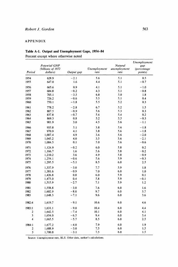
rate. These quarters are 1948:4, 1953:4, 1957:3, 1960:1, 1970:3, 1974:2, and 1979:3. These quarters occur at varying intervals after the peak designated by the National Bureau of Economic Research for each cycle, because the unemployment rate was operating in those peak quarters at vaLying amounts below the natural rate of unemployment.'0 (Data for the output and unemployment gaps from 1954 to 1984 are shown in appendix table A-1.)

Table 2 displays the growth rates between these benchmark quarters for real GNP and each of the components of identity 4. Since we define "potential real GNP" as the economy's real output when operating at the natural rate of unemployment, the first column of table 2 provides estimates of the growth rate of potential (or natural) real GNP over each major cycle between 1948 and 1979. Familiar phenomena include the rapid potential growth achieved during the Korean War cycle, a potential growth rate close to 3.0 percent in the remainder of the 1950s and close to 3.75 percent between 1960 and 1974, followed by a deceleration to 3.25 percent after 1974. A key question addressed below is, what has happened to the growth rate of potential real GNP after 1979? To facilitate comparison, the cyclically corrected values, derived from the subsequent analysis, are displayed in the bottom line of table 2, but their discussion is postponed for now.

Because the natural rate of unemployment series, used to establish the benchmark quarters, gradually increases during the postwar period, the corresponding natural rate of employment declines. Most of this decline shows up in the second column of table 2 in the 1957-60 interval. Between the other benchmark quarters, the change in the employment rate was negligible. The third column displays the growth rate of productivity between benchmark years, with a rate of 2 percent per year or faster before 1970, 1.5 percent between 1970 and 1974, and 1.1 percent between 1974 and 1979. Our choice of benchmark quarters assigns the sharp decline in productivity in the first half of 1974 to 1970-74 instead of 1974-79, and this partly accounts for the two-step phasing in of the productivity growth slowdown of the 1970s.

Other features of the postwar growth process can be identified in the

10. For instance at the NBER peak in 1969:3 the actual unemployment rate was 2.0 points below the estimated natural rate, but in 1973:4 it was only 1.0 point below. This accounts for the fact that our benchmarks in 1960:1 and 1979:3 occur before the NBER peak quarter.


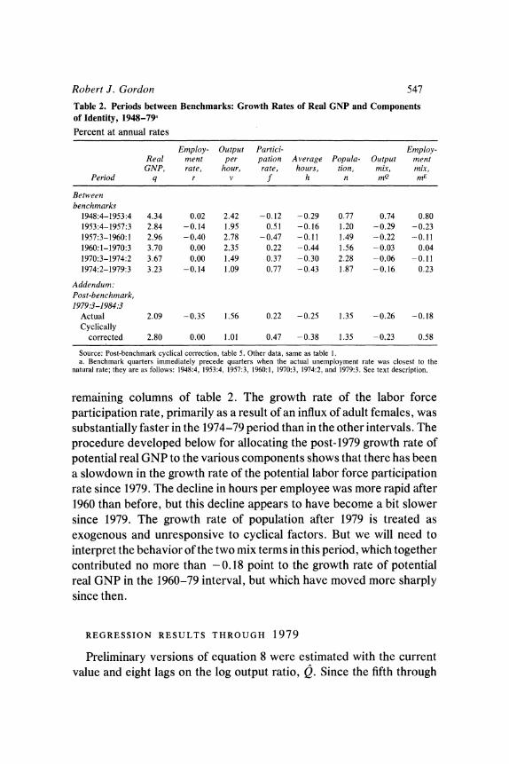
Table 2. Periods between Benchmarks: Growth Rates of Real GNP and Components of Identity, 1948-79a

Percent at annual rates

Employ- Output Pasrtici- Employ- Real ment per pation Average Popula- Output ment GNP, rate, hour, rate, hoiurs, tion, mix, mix,

Period q r v f h n mQ mE

Between benchmarks

1948:4-1953:4 4.34 0.02 2.42 -0.12 -0.29 0.77 0.74 0.80 1953:4-1957:3 2.84 -0.14 1.95 0.51 -0.16 1.20 -0.29 -0.23 1957:3-1960:1 2.96 - 0.40 2.78 - 0.47 -0.11 1.49 - 0.22 -0.11 1960:1-1970:3 3.70 0.00 2.35 0.22 -0.44 1.56 -0.03 0.04 1970:3-1974:2 3.67 0.00 1.49 0.37 -0.30 2.28 -0.06 -0.11 1974:2-1979:3 3.23 -0.14 1.09 0.77 - 0.43 1.87 -0.16 0.23

Addendum: Post-benchmark, 1979:3-1984:3

Actual 2.09 -0.35 1.56 0.22 -0.25 1.35 -0.26 -0.18 Cyclically

corrected 2.80 0.00 1.01 0.47 -0.38 1.35 -0.23 0.58

Source: Post-benchmark cyclical correction, table 5. Other data, same as table 1. a. Benchmark quarters immediately precede quarters when the actual unemployment rate was closest to the

natural rate; they are as follows: 1948:4, 1953:4, 1957:3, 1960:1, 1970:3, 1974:2, and 1979:3. See text description.

remaining columns of table 2. The growth rate of the labor force participation rate, primarily as a result of an influx of adult females, was substantially faster in the 1974-79 period than in the other intervals. The procedure developed below for allocating the post-1979 growth rate of potential real GNP to the various components shows that there has been a slowdown in the growth rate of the potential labor force participation rate since 1979. The decline in hours per employee was more rapid after 1960 than before, but this decline appears to have become a bit slower since 1979. The growth rate of population after 1979 is treated as exogenous and unresponsive to cyclical factors. But we will need to interpret the behavior of the two mix terms in this period, which together contributed no more than - 0.18 point to the growth rate of potential real GNP in the 1960-79 interval, but which have moved more sharply since then.

REGRESSION RESULTS THROUGH 1979

Preliminary versions of equation 8 were estimated with the current value and eight lags on the log output ratio, Q. Since the fifth through

C) cn lr 1. cn cn C) a\ o t ( m w.l lr - "t C) ct n cn C) ,. OC \ 'It eq 0 - C CD 0CD D C

e C

o St N X o o o o o ̂ V t

ei1. 00 -0~a cq 110 -00 -cq110 ell0 '0

00000l~a\00 0 0 0000a\e

C I I I I

-00en00 r' 0 00 ~ ~ ~ 0

ONo oo oeX i ON 0 00 0U:' ro0oN 00 -0 r . c 00 0 0 0 el elo 00000 0 0 0

O I II e I I

.U~~~~~~~~~~~~~~~~~~~~~~~~~~.

U W ~~~* * * rU rv '_,N 00 N 0000 N ^ O

eS W0~e 00<1s- O -

g t~~~~~~~~~~~~~~~~~~~~~~~~~~~~t 00

Y .o ~ ~~* * *

v ~ ~ N 4 .I NONrO01- 0 r0 0. u E M cr cd ? o^oot o

F ~~~~.j_< cis w 4 o .=o 0 00000 000 r~~~ 0 --

- ;- o~~~~~ **

- o) Z 4)

Q ~~~~~~~~~~~~~~~~n

o W ~~~* * * * * *m S~~lr~ ^e l N tr N rw - e lN

o ^ i I I

u 0-~~~~~~~~~~~~~~~

o S Q 0-lr_

.w~~~~~~~~~~~~~~~~~~~~~~~~~~~~~~~~~~~~~~~~~~~~~~~~~~4 .= ' '

. Q i t i X q X Q 8 9 B ] M~~~~~~~~~~~~~ c


eighth lags were jointly insignificant, the equations were reestimated without these terms. Each of the equations displayed evidence of significant positive serial correlation, however, and so we do not report the individual coefficients here.

The serial correlation problem can be eliminated by adding four lagged values of the dependent variable to each equation. Thus, in place of seven equations in the form of equation 8, I estimate seven equations in the form of

4 4

(10) Yit = ai + > ciS Yi ts+ b is + u,it

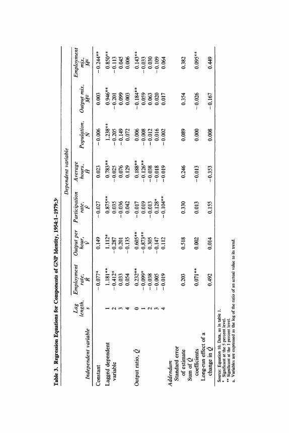
where, as in equation 8, Yi stands for one of the seven components of the output identity. This approach has a disadvantage: because a different set of lagged dependent variables enters each equation, the adding-up property of equation 8 is not preserved. The long-run responses of Y to Q in equations specified as in equation 10 are displayed on the last line of table 3. These responses sum to 0.6, so that the loss of the adding-up property is a moderately serious problem. The small long-run effect shown for output per hour indicates there is virtually no permanent productivity bonus to be enjoyed from a period of high utilization of the economy's resources; there is only a transitory productivity bulge associated with an increase in the output ratio. 1 I

The remainder of table 3 shows the individual coefficients in the format of equation 10 for each of the seven components of the output identity. In each case the first lagged dependent variable is highly significant, indicating that the dynamic relationship between the seven components and the output ratio involves a response of the change in each component to the change in the output ratio. The first-difference relationship is particularly evident in the columns for output per hour and for hours per employee. In these columns note that the coefficient on the output ratio lagged once is significantly negative and about the same order of magnitude as the positive coefficient on the current value. A test for the joint exclusion of current and lagged output values showed output was significant in all equations except that for population.

11. This result conflicts with my previous finding that there is a permanent productivity bonus. See Robert J. Gordon, "The 'End-of-Expansion' Phenomenon in Short-Run Productivity Behavior," BPEA, 2:1979, pp. 447-61. The long-run effect appears to turn on whether the dependent variable is total hours, as in that paper, or productivity itself, as in this paper.


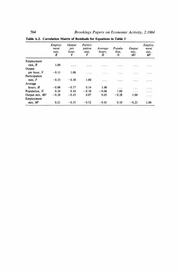
In table 3 two features of the employment-rate column, the Okun's law equation, are evident. First, the long-run Okun's law coefficient, which is the entry in the last row, is close to 0.5, not the 0.33 popularized by Okun's original work."2 Second, leaving aside the equation for population, which is included only for symmetry, the standard error in the Okun's law equation is lower than for any of the other equations. This occurs because of negative correlations among the residuals in some of the other equations. For instance, a decline in productivity is accompanied not only by an increase in hours but also by an increase in the two mix-effect terms. Such negative correlations may explain why Okun's law has remained relatively reliable over the years. (The correlation matrix of the residuals of the table 3 equations is presented in appendix table A-2.)

The Post-1979 Growth Rate of Potential Real GNP

MINIMIZING THE POST-1979 ERROR

IN THE EMPLOYMENT RATE

The estimated Okun's law relationship in table 3 can be used to estimate the growth rate of potential output since 1979. Because the Okun's law equation has a relatively low standard error before 1979, there is a presumption that it may also track the relationship between the employment rate and the output ratio, Q, since 1979. An additional advantage of choosing the employment rate equation for this exercise is that its trend value, the natural rate of employment, was virtually constant in the five years before 1979 and can be presumed to have changed little since 1979. In contrast, several of the other components of the identity have significant trends between benchmarks and, as we shall see, some of these trends have changed since 1979.

The basic idea of using an Okun's law equation to track potential real GNP growth is straightforward, but several choices must be made regarding the details of implementation. We must search for a growth

12. This result conflicts with Clark's finding that Okun's original estimate of one-third is correct. The discrepancy may result from restrictions Clark imposes on the shape of the lag distribution and on the form of the serial correlation coefficients, in contrast with the unrestricted format in table 3. Also, Clark's equations include leading values of the output ratio variable.


rate of potential real GNP, q*, that minimizes the post-1979 error in an equation for the employment rate. The first choice that must be made is the time interval for the error. The obvious choice is the root mean squared error over the entire post-1979 period. This places relatively more weight on observations in 1983-84 than in 1980-82, since an incorrect value of q* would cause potential real GNP to drift away from its "true" value as time goes on. For instance, a value of q* that is 1 percentage point per year too high would cause the output ratio, Q, to be five percentage points too low by mid-1984, and the implied employment rate for mid-1984 would be much lower than the actual observed employment rate.

The criterion based on the root mean squared error over the 1979-84 period differs from the related exercise carried out by Clark. While I choose a single value for q* by minimizing the error over the full five- year period, Clark chooses a different growth rate of q* each quarter that minimizes the error in an Okun's law equation in that particular quarter. 13 The result of Clark's procedure is a highly variable time series for q* instead of the fixed growth rate between benchmarks that results from my procedure. An undesirable side effect of Clark's method is that it translates temporary errors in the Okun's law equation directly into variations in q*. In 1981-82 the unemployment rate rose more rapidly than Okun's law can explain with a fixed value of q* and in 1983-84 fell more rapidly, so Clark's method reaches the conclusion that q* grew in 1982 and fell in 1983-84.

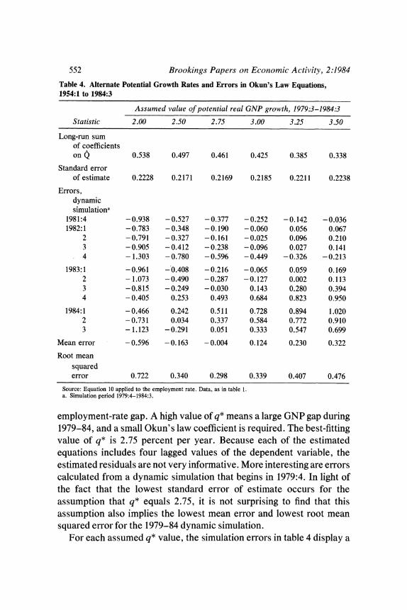
The Okun's law equation presented in table 3 provides a set of coefficients that can be used to calculate the employment rate implied by alternative GNP gaps corresponding to different assumed growth rates of potential real GNP, q*, since 1979. Table 4 displays six sets of long-run coefficient estimates and standard errors of estimate, corresponding to six different assumptions about the post- 1979 growth rate of q*, varying from 2.0 to 3.5 percent per year. In each of the six columns, the post-1979 trend value of the employment rate is assumed to be fixed at 94.0 percent.

Note first that the long-run sum of coefficients on Q varies inversely with the assumed value of q*. This is intuitively sensible, because a low assumed value of q* means a small GNP gap during 1979-84, so that a large Okun's law coefficient is then required to "explain" the observed

13. Clark, "Okun's Law and Potential GNP."


Table 4. Alternate Potential Growth Rates and Errors in Okun's Law Equations, 1954:1 to 1984:3

Assumed value of potential real GNP growth, 1979:3-1984:3

Statistic 2.00 2.50 2.75 3.00 3.25 3.50

Long-run sum of coefficients on Q 0.538 0.497 0.461 0.425 0.385 0.338

Standard error of estimate 0.2228 0.2171 0.2169 0.2185 0.2211 0.2238

Errors, dynamic simulationa

1981:4 -0.938 -0.527 - 0.377 -0.252 -0.142 -0.036 1982:1 - 0.783 -0.348 -0.190 -0.060 0.056 0.067

2 -0.791 -0.327 -0.161 -0.025 0.096 0.210 3 - 0.905 -0.412 - 0.238 -0.096 0.027 0.141 4 - 1.303 -0.780 -0.596 -0.449 -0.326 -0.213

1983:1 -0.961 -0.408 -0.216 -0.065 0.059 0.169 2 - 1.073 -0.490 -0.287 -0.127 0.002 0.113 3 -0.815 - 0.249 - 0.030 0.143 0.280 0.394 4 -0.405 0.253 0.493 0.684 0.823 0.950

1984:1 -0.466 0.242 0.511 0.728 0.894 1.020 2 -0.731 0.034 0.337 0.584 0.772 0.910 3 - 1.123 -0.291 0.051 0.333 0.547 0.699

Mean error - 0.596 - 0.163 -0.004 0.124 0.230 0.322

Root mean squared error 0.722 0.340 0.298 0.339 0.407 0.476

Source: Equation 10 applied to the employment rate. Data, as in table 1. a. Simulation period 1979:4-1984:3.

employment-rate gap. A high value of q* means a large GNP gap during 1979-84, and a small Okun's law coefficient is required. The best-fitting value of q* is 2.75 percent per year. Because each of the estimated equations includes four lagged values of the dependent variable, the estimated residuals are not very informative. More interesting are errors calculated from a dynamic simulation that begins in 1979:4. In light of the fact that the lowest standard error of estimate occurs for the assumption that q* equals 2.75, it is not surprising to find that this assumption also implies the lowest mean error and lowest root mean squared error for the 1979-84 dynamic simulation.

For each assumed q* value, the simulation errors in table 4 display a


consistent pattern. The errors for 1982:4, the trough quarter of the 198 1- 82 recession, always have the largest negative values, and the errors for 1983:4 and 1984:1 have the largest positive (or smallest negative) values. This pattern of errors reinforces the impression that the employment rate has risen "too rapidly" since the recession trough, partly because it was "too low" at the trough. The difference between the errors in 1982:4 and 1984:3 is 0.65 percentage points, compared with an actual increase of 3.46 percentage points in the employment rate during the same interval. Thus about one-fifth of the increase in the employment rate is left unexplained in this approach.

OTHER COMPONENTS OF THE OUTPUT IDENTITY SINCE 1979

Having concluded that potential real GNP has grown at a rate of about 2.75 percent since 1979, the next step is to account for this growth by the separate components of the output identity-productivity, hours, participation, and the rest. In doing so, pre-1979 trends for the separate components cannot be used, because these may have changed; and observed post-1979 trends are contaminated by cyclical effects, because the economy has not yet reached a natural-employment benchmark. Therefore I developed a modified search procedure to identify the post- 1979 trends of six components of the identity, with no trend change assumed for the seventh component, the employment rate, R, because I treat the natural unemployment rate as constant at 6.0 percent during 1979-84. Given the 2.75 percent annual growth rate of potential real GNP determined in table 4, the equations for the six components of the identity from the second through seventh dependent variables of table 3, all estimated over the 1954:1-1979:3 period, are simulated for the interval 1979:4-1984:3. The fitted value of this dynamic simulation is the detrended level of each component of the identity, expressed as a function of its own lagged simulated values and the current and lagged values of the output ratio:

4 4

(11) Yi, a i + > ci Y + E b Qt + it

Here equation 11 is identical to equation 10 except for the primes on the detrended Y terms, which indicate simulated values for the 1979-84 period. The output ratio terms are constructed using the pre-1979 trends

s: w o- o-rie ' -e^ o~ o o-o

00 t a,\ c en 00 0000"t r n , W 0 -0

C) 0e ' r IS OO 0-' ,

+

tE~~i~ ~ oo ^ ^ t oo5 oo 000

0 II I I I I I I I I I I I I 0 S

_ oo

U2 L- Z- .

* eoo en ~ ~ e ~~ ~ ~ 0r~~~-~-

*I -

en 0 0 0-W)'C 'I I

W 0 rie0r 00 00 00

N

m . Cm

i~~~ '; ONbOO o- X

F~~~~~~~~~~~~~~~e en I en "t *_t en 0 ? O. N It 'IC^^

C,~~ 00 0000 000

S AR A I I > I ~~~I II l i I I I I I I

E 0d

U2~~~~~~~~~~~~~~~~~~~~~~~~~~~~~~~~~~~~~~~~~~~~~~~~~~~C o

0 --

k4~~~~II4

N 00 00 00 00 00 0

m x 0>

O NO^N ON ON O ON ONOOO


for potential output growth, q*, shown in table 2 and 2.75 percent per year as the potential output growth rate for 1979-84.

Alternative values for the trend value for each component in each quarter, Yi*, were computed by searching a grid of possible values for the 1979-84 growth rate of Yi*, for example, 0.00, 0.05, and so on. These alternative values, Yi*, were then compared with the values of the trend, Yi*', implied by the observed actual values, Yit, and the simulated detrended values from equation 11, that is, Yi',:

(12) Y.= i i

exp Yi't

The exponent enters because of our original definition of all detrended variables in log form, that is, Y = ln (Y/Y*). The grid is searched for small increments above and below the previous 1974-79 trend to determine the value of the 1979-84 trend that minimizes the sum of the squared differences between the alternative constructed trend values along the grid, Yi*t and Y: ' of equation 12. Thus we minimize the sum of the squared errors, that is, the sum Of (Yt t Y:')2, for each of the six components of the identity.

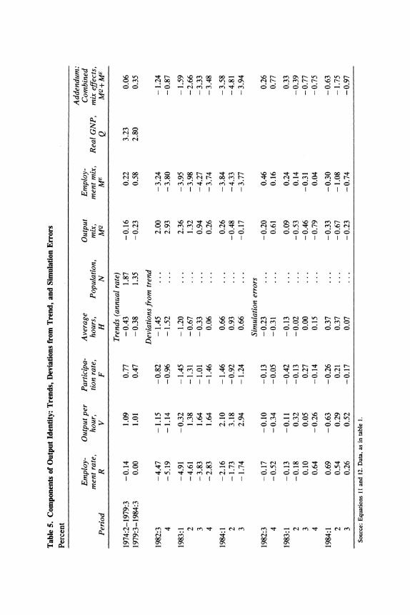
Table 5 is arranged with a column for each component of the identity and is divided into three sections. The top section shows the value of the optimal constructed 1979-84 trend for each component, Yi*, and com- pares it with the previous trend between the 1974:2 and 1979:3 benchmarks, taken from table 2. The middle section of table 5 shows the calculated log deviations between the actual observed values and these optimal trends, thatis, ln (Yit/ Yi*t). The bottom section shows the dynamic simulation errors from equation 11 that are the key ingredient in finding the optimal post-1979 trends.

The most interesting results are for productivity growth in the second column of table 5. The top section shows that cyclically adjusted productivity growth in the nonfarm private business sector in 1979-84, 1.01 percent, was almost the same as the 1.09 percent trend experienced during the 1974-79 interval. This is the same conclusion recently reached by Clark.14 There is no evidence at all that the productivity growth slowdown of the 1970s was transitory, at least in the data available through 1984:3.

14. Peter K. Clark, "Productivity and Profits in the 1980s: Are They Really Improv- ing?" BPEA, 1:1984, pp. 133-67.


Productivity growth in 1984:2 and 1984:3 soared just about 3 percentage points above the estimated 1.01 percent trend line, as shown in table 5, middle section, second column. But the relatively small simulation errors, bottom section, second column, indicate that the excess of actual productivity over the estimated trend line was a normal cyclical phenomenon and can be explained by the fact, evident in the regression equation displayed in table 3, that productivity growth responds positively to the growth of the output ratio, not its level, and thus was unusually high in response to the rapid pace of the 1983-84 recovery. As actual output growth recedes toward its estimated potential rate of 2.75 per year, this analysis predicts that the deviation of productivity from trend (shown in the middle section of table 5) will recede toward zero. During this process we could observe several quarters of zero or even negative productivity growth, a possibility confirmed by the government's preliminary estimate of zero productivity growth in 1984:3.

Fortunately the assumed annual rate of q*, 2.75, yields a set of trend estimates for the components of the identity that sum to 2.80 percent, very near the assumed value. The top section of table 5 also shows that two factors, slower trend growth in participation and in population, have contributed to slower growth in potential real GNP since 1979. Together these two factors have reduced q* by 0.79 percentage points, and their effect has been only partially offset by a slightly slower decline in hours (0.05 points) and a more positive trend in the sum of the two mix effects (a shift from 0.06 to 0.36 points). Overall, the growth rate of potential real GNP slowed by 0.43 points from 1974-79 to 1979-84, and with unemployment already at 7.5 percent this will soon place a constraint on the feasible path of actual real GNP.

The middle section of table 5 shows that the deviation from trend of average hours, like that of productivity, has been positive in 1984. As table 3 showed, hours respond strongly to the rate of change of real GNP, and thus hours, like productivity, have been boosted by the rapid pace of the economic recovery to date. In contrast, the participation rate has made large and continuing negative contributions to the log output ratio (GNP gap) during the past two years. The errors in the bottom section of table 5 are not large, indicating that this pattern of participation is tracked fairly accurately by the dynamic simulations of the 1954-79 equations.

Taken together, the mix-effect variables are not entirely satisfactory.


Output mix shows a cyclical pattern that brought it from a large positive at the end of the recession back to near zero in recent quarters. The modest errors in the bottom of the table indicate this pattern was predictable. Although the large persistent negative deviations from trend in the employment-mix term are typical and occur in every business cycle, the large negative simulation errors in the latest quarters indicate that the behavior of the two employment measures has been unusual recently. 15

We can now use the simulation errors in the bottom section of table 5 to ask, Why was the unemployment rate so high in late 1982? And why did it decline so rapidly in 1983-84? Although the sum of the errors of the first through seventh columns is not zero, because these equations do not observe an exact adding-up property, the sum varies within a relatively narrow range between -0.34 and -0.46. This allows us to match large errors in the employment-rate column with correspondingly large errors of the opposite sign in one or more of the other columns. Because the behavior of the employment mix does not appear to have been captured well by the present model, and because the employment- mix errors may involve data problems instead of behavioral issues, we will confine our attention, for now, to the other elements of the identity.

Between the trough of the recession, in 1982:4, and 1984:3, the unemployment rate fell from 10.6 percent to 7.5 percent, corresponding to a rise in the employment rate of 3.5 percentage points. The simulation errors of table 5 indicate 0.8 point of this rise was not predicted by the Okun's law equation (first column), so that 2.7 points, or 80 percent of it, was predicted from the behavior of real GNP.

Of the 0.8 point error, it appears the employment rate was 0.5 point too low in 1982:4. In that quarter, a 0.6 point positive error in the output- mix term indicates total real GNP was unusually high relative to nonfarm business real GNP. In other words, the output ratio, Q, based on total real GNP, made the economy look more prosperous and predicted higher employment than can be explained by normal cyclical relations.

The rapid decline in unemployment and corresponding increase in the employment rate in 1983:4 and 1984:1 show up as positive simulation

15. Until recent months, commentators noted the more rapid rise in E than in EB as an interesting phenomenon. See "An Economic Indicator Takes on New Luster," Business Week (July 23, 1984), p. 20. However, by 1984:3, employment growth during the recovery had come together in the two measures.


errors in the first column. 16 These positive errors have as their counterpart negative errors in productivity, participation, and output mix, again ignoring the employment-mix errors for now. The rapid decline in unemployment appears to be connected with relatively slow growth in productivity and participation and slow growth in total real GNP relative to nonfarm business real GNP. By 1984:3, errors are relatively small except for productivity, which is high relative to prediction in that quarter. Over the entire interval from 1982:4 to 1984:3, the productivity errors move in the same direction as the employment rate errors, so they add to, rather than explain, the mystery of why unemployment declines so much. By contrast, the output-mix errors, taken alone, do offset the employment errors for this interval and thus contribute to an explanation of them.

Turning now to the employment mix, large negative errors in the two latest quarters indicate that total employment in the household survey grew rapidly relative to nonfarm employment reported by establishments. This could reflect an underreporting of new establishments, which could also understate output. Or it could be a transitory phenomenon, with no such meaning.

The simulation errors in table 5 are linked together by an identity, and so the connections discussed above do not imply causation. Some of the offsetting errors in particular components of the identity are to be expected and are consistent with the negative correlations among errors for the 1954-79 period displayed in the correlation matrix of appendix table A-2. In particular, some correlations involve the employment-mix term, whose behavior has been puzzling in the present recovery according to this analysis. The offsetting productivity and employment-mix errors in 1984:3, for instance, are consistent with the negative correlation between those two components observed in 1954-79.

Combining the two mix effects reveals a strong trend in their combined errors in the past two years. We can offer some conjectures as to the observed shifts in the combined mix effect. Recall that the output-mix effect is defined as MQ = Q/QB, where the B superscript refers to the

16. The simulation errors in the first column of table 5 differ from those in the third column of table 4, because the table 5 errors are based on coefficients from an equation estimated for the 1954-79 period, whereas those in table 4 use coefficients estimated for 1954-84.


nonfarm private sector. The employment-mix effect is ME = EBIE. Thus the two effects together are

(13) MQME = QIE QB/EB '

that is, the ratio of average output per employee in the total economy to average output per employee in the nonfarm private business sector. Negative shifts in equation 13 might have occurred if there had been a shift in the economy's output mix from the higher-productivity nonfarm private sector to the lower-productivity government and farm sectors, but this does not seem to provide a plausible explanation. 17 Thus we fall back on the possibility of data measurement errors to explain the decline in the productivity ratio expressed in equation 13. This could have occurred if household employment, E, were measured correctly, while the remaining three components that rely to some extent on establishment surveys (Q, QB, and EB) were understated due to the undersampling of new firms. If this were true, it would account for underpredicting the decline in the unemployment rate by the fact that the real GNP rise has been understated in official data. It is likely that the validity of this hypothesis cannot be assessed for several more years until there is a major benchmark revision of the real GNP data. 18

In light of the evidence that the productivity trend for total private nonfarm business has not quickened, it is worth comparing that aggregate sector's productivity with the productivity performance of the manufacturing sector alone. By converting published index numbers into actual levels, the aggregate private nonfarm data are divided into productivity indexes for manufacturing and nonfarm nonmanufacturing separately.

17. Published tables of the Bureau of Labor Statistics indicate no major difference between productivity growth in the private business and nonfarm private business sectors, indicating that the farm sector does not contribute to the puzzle. As for the government sector, the national income and product accounts (comparing tables 6.1 with 6.8B) indicate that real GNP per full-time-equivalent employee in the nonfarm private sector is more than 50 percent higher than in the government sector. Thus the unusually slow growth of government-sector real GNP in 1983-84 should have created a positive rather than a negative productivity mix effect.

18. Such a data revision could take as long as seven years, judging from the example of the recent $58 billion upward revision of 1977 GNP reported in Gerald F. Donahoe, "The National Income and Product Accounts: Preliminary Revised Estimates, 1977," Survey of Current Business, vol. 64 (May 1984), pp. 38-41.


The annual growth rates for all three between the benchmark quarters and since 1979:3 are as follows:

Nonfarm Total private Manu- nonmanu-

nonfarm facturing facturing

1948:4-1953:4 2.4 2.7 2.4 1953:4-1957:3 2.0 2.4 1.6 1957:3-1960:1 2.8 2.2 3.1 1960:1-1970:3 2.4 2.6 2.3 1970:3-1974:2 1.5 3.6 0.5 1974:2-1979:3 1.1 2.1 0.7 1979:3-1984:3 1.6 3.0 1.0

Productivity outside manufacturing slowed sharply after 1970, well before the first oil shock. All the slowdown in aggregate nonfarm productivity in this interval comes from this sector; productivity speeded up in manufacturing. Even in the post-OPEC interval of 1974:2-1979:3, manufacturing productivity growth is only moderately below its performance in the 1950s and 1960s, while outside manufacturing the productivity trend is still very slow. Since 1979:3 all three sectors show faster productivity growth, although the statistical analysis for the aggregate nonfarm sector attributes all of this speedup to the cyclical recovery and none to a quickening trend. Determining whether the speedup to 3.0 percent growth in manufacturing productivity in this latest period represents some improvement in trend requires a further statistical analysis and, probably, more quarters of observation.

Conclusion

The point of departure for this paper was the surprisingly rapid, 3.1 point decline in the aggregate unemployment rate during the first seven quarters of the 1983-84 recovery. Analysis of potential output growth over this period and the Okun's law relationship between unemployment and output indicates that a 2.4 point decline in unemployment could have been expected given the rapid rise in GNP and the modest growth of potential GNP in this period. The remaining 0.7 point decline occurred because, relative to prediction, the unemployment rate was


about 0.5 point "too high" in 1982:4 at the trough of the recession and about 0.2 point "too low" in 1984:3. It was a bit more than 0.5 point "too low" during 1983:4-1984:2. Analysis of the output identity reveals several factors that have been the counterparts of these surprises in the unemployment rate: a disappointing productivity performance in 1983:4- 1984:1, an unusual rise in nonfarm business output relative to GNP during 1983, and an unexplained surge in 1984:2 and 1984:3 in the ratio of household to establishment employment.

The analysis of historical Okun's law relationships between unemployment and output yields as a byproduct several findings on the growth of potential real GNP and productivity. It appears that natural or potential real GNP, Q*, which measures how much the economy can produce when operating at its natural unemployment rate, roughly 6.0 percent since 1975, grew by 3.75 percent per year between 1960 and 1974, 3.35 percent per year between 1974 and 1979, and 2.80 percent per year since 1979. The majorfactors contributing to a slowdown in potential output growth after 1979 are slower growth in the working-age population, owing to the decline in the birth rate that occurred in the 1960s, and slower growth in the labor force participation rate, indicating that the rapid influx of adult women into the labor force that characterized the late 1970s may have passed its peak.

The analysis indicates that the relatively rapid productivity growth in the period 1983:1 to 1984:2 was a normal cyclical phenomenon, the counterpart of the rapid output growth that occurred in the same six quarters. The cessation of productivity growth in 1984:3, the counterpart of relatively slow ouput growth in that quarter, supports the pessimistic assessment offered here.

The finding that aggregate productivity growth has not revived since 1979, after adjustment for normal cyclical effects, has important implications for alternative hypotheses that have been developed to explain the post-1973 slowdown in productivity growth. Several of these hypotheses, by focusing on factors that were adverse in the 1970s but have improved in the 1980s, suggest that we now should be witnessing an amelioration of the productivity slowdown. These hypotheses include the impact in the 1970s of higher oil prices, higher prices of other raw materials, slower capital accumulation, and more stringent government regulation. Another approach, Nordhaus's "depletion hypothesis," based on a decline in innovation and a general "running out of ideas,"


does not call for any turnaround in the 1980s and seems to be supported by the evidence in this paper that the nonfarm private productivity trend has not revived when 1979-84 is compared with 1974-79.19

The analysis in this paper contains some further implications for policymakers and policy debates. First, the regression results show that a permanent increase in the economy's use of its resources causes only a temporary increase in productivity above its long-run trend, not a permanent increase. Thus any argument for raising the economy's utilization rate must rest on the benefits of job creation rather than on the benefits of a permanent productivity bonus. Second, the relatively slow 2.8 percent growth rate estimated for potential real GNP since 1979 defines the output growth rate that is consistent with a constant unemployment rate; it will constrain the growth of output once the economy arrives at its natural unemployment rate of roughly 6 percent. As of 1984:3, however, there is still slack in the economy, with the actual unemployment rate 1.5 percentage points higher than the assumed natural rate, and the actual level of real GNP 3.1 percent below the estimated level of potential real GNP.

Finally, this analysis raises serious doubts about supply-side analyses that predicted a flowering of productivity and work effort as a result of the tax rate reductions that have been put in place. After cyclical correction, there appears to have been no improvement in productivity growth in the nonfarm private sector as a whole. Any improvement that may have occurred in the manufacturing sector, where actual productivity gains have been relatively large, has been offset by a deterioration elsewhere in the economy. As for the predicted response in work effort, there is no important change in the downward trend in average hours, and there has been a slowdown of 0.3 percentage points in the trend growth rate of labor force participation between 1974-79 and 1979-84.

19. William D. Nordhaus, "Economic Policy in the Face of Declining Productivity Growth," European Economic Review, vol. 18 (May-June 1982), pp. 131-57.


APPENDIX

Table A-i. Output and Unemployment Gaps, 1954-84 Percent except where otherwise noted

Unemployment Potential GNP Natural gap (billions of 1972 Unemployment unemployment (percentage

Period dollars) Output gap rate rate points)

1954 628.9 -2.1 5.6 5.1 0.5 1955 647.0 1.6 4.4 5.1 -0.7

1956 665.6 0.9 4.1 5.1 - 1.0 1957 684.8 -0.2 4.3 5.1 -0.8 1958 705.1 -3.5 6.8 5.0 1.8 1959 726.2 -0.6 5.5 5.1 0.4 1960 750.1 -1.8 5.5 5.2 0.3

1961 778.2 -2.8 6.7 5.2 1.5 1962 807.5 -0.9 5.6 5.3 0.3 1963 837.8 -0.7 5.6 5.4 0.2 1964 869.3 0.8 5.2 5.5 -0.3 1965 901.9 3.0 4.5 5.6 - 1.1

1966 935.8 5.1 3.8 5.6 -1.8 1967 970.9 4.1 3.8 5.6 - 1.8 1968 1,007.4 4.9 3.6 5.6 -2.0 1969 1,045.2 4.0 3.5 5.6 -2.1 1970 1,084.5 0.1 5.0 5.6 -0.6

1971 1,124.9 -0.2 6.0 5.8 0.2 1972 1,166.7 1.6 5.6 5.8 -0.2 1973 1,210.2 3.6 4.9 5.8 -0.9 1974 1,254.1 -0.6 5.6 5.9 -0.3 1975 1,295.5 -5.1 8.5 6.0 2.5

1976 1,337.9 - 3.0 7.7 5.9 1.8 1977 1,381.6 -0.9 7.0 6.0 1.0 1978 1,426.8 0.8 6.0 5.9 0.1 1979 1,473.0 0.4 5.8 5.9 -0.1 1980 1,515.9 -2.7 7.1 5.9 1.2

1981 1,558.8 - 3.0 7.6 6.0 1.6 1982 1,602.9 -8.0 9.7 6.0 3.7 1983 1,648.3 -7.1 9.6 6.0 3.6

1982:4 1,619.7 -9.1 10.6 6.0 4.6

1983:1 1,631.1 -9.0 10.4 6.0 4.4 2 1,642.5 -7.4 10.1 6.0 4.1 3 1,654.0 -6.5 9.4 6.0 3.4 4 1,665.5 -5.7 8.5 6.0 2.5

1984:1 1,677.2 -4.0 7.9 6.0 1.9 2 1,688.9 - 3.0 7.5 6.0 1.5 3 1,700.8 -3.1 7.5 6.0 1.5

Source: Unemployment rate, BLS. Other data, author's calculations.


Table A-2. Correlation Matrix of Residuals for Equations in Table 3

Employ- Output Partici- Employ- ment per pation Average Popula- Output ment rate, hour, rate, hours, tion, mix, mix,

R V F H N' MQ E

Employment rate,R 1.00 ... ... ... ... ... ...

Output per hour, v -0.11 1.00 ... ... ... . .

Participation rate, F - 0.33 -0.18 1.00 ... ... ... ...

Average hours, H -0.08 - 0.57 0.14 1.00 . .. ...

Population, N ~ 0.10 0.10 -0.18 -0.06 1.00 ...

Output mix, MfQ -0.18 -0.43 0.07 0.03 -0.28 1.00 ... Employment

mix, M~IE 0.21 -0.35 -0.52 -0.01 0.10 -0.23 1.00

Comments and Discussion

Peter K. Clark: In this paper, Robert Gordon has attacked an important fiscal policy issue: what is the trend rate of growth in U.S. real output? If the underlying growth rate is high, then projecting higher future output and lower future federal deficits may be justified. Conversely, if the underlying trend is weak, then projections of slower growth and higher future deficits are more appropriate.

Gordon finds that the trend growth rate of real GNP has been about 2/4 percent per year, well below the postwar average of 3? /2percent, and on the pessimistic end of the range of estimates one usually hears. This figure is generated by a complicated procedure that combines an arbitrary estimate of Okun's law for 1954-79 with a nonlinear search routine to find the best-fitting growth rate for 1979-84.

A simpler route to the same result is to estimate Okun's law in first- differenced form, as shown below (standard errors in parentheses, sample period 1954:1-1984:2). The ratio of the constant term to the sum of the output coefficients in such an equation provides an estimate of the growth rate of trend GNP; the dummy variable D80 (which equals 0 before 1980: 1 and equals 1 thereafter) generates an estimate of the decline in the trend output growth at the turn of the decade.

AU, = 0.416 - 0.099 D80 - 24.9 Alog Y, - 16.0 AlogY,1 (0.03) (0.06) (2.2) (2.3)

- 6.2 A10gY,-2 (2.2)

= 0.74 Standard error of estimate = 0.23 Durbin-Watson = 1.69

According to this regression, trend output growth has declined significantly in the 1980s-from 3.6 percent per year before 1980 to 2.7

565


percent per year thereafter. However, four-and-a-half years is not a very long time for estimation of a new output trend, and a rate anywhere from 2.2 to 3.2 percent is consistent with the unemployment and real output statistics since 1979. A substantial fraction of the reduction in trend output growth can be traced to the steep decline in unemployment in the last year and a half; if the sample period is truncated at the end of 1982, the estimated trend real GNP growth rate for the 1980s is 3.3 percent per year, with a range of 2.7 to 3.9 percent fitting the data fairly well.

Given its impact on the trend output growth rate, the recent decline in unemployment deserves further scrutiny. Gordon attempts to do this by using the linear regression decomposition that I introduced in an earlier paper on Okun's law. However, one of the main conclusions in that paper was that unemployment is more closely linked to the cyclical movements in real output than other components (such as productivity, labor force participation, and work weeks) of the identity that relates employment to real GNP. This implies that an investigation of the large errors in these components is unlikely to reveal the cause of the smaller errors in Okun's law, except in the vacuous sense that they will meet one linear constraint to make an identity hold. Thus, it is no surprise that Gordon ends up attributing the 1983-84 unemployment decline to shifts in his employment- and output-mix terms, which have erratic cyclical behavior.

Probably the best explanation for the recent decline in the unemployment rate is that reductions in real GNP during recession and sharp increases in real GNP during the early stages of recovery each generate larger movements in the unemployment rate than would be predicted by Okun's law. For example, in the 1957-58, 1969-70, and 1974-75 recessions, the unemployment rate rose an average of 0.7 percentage point more than predicted by Okun's law. In the ensuing recoveries, it declined 0.3 percentage point more than the Okun's law prediction (this figure rises to 0.6 percentage points if the slow recovery in 1971 is excluded). In 1981-82, the unemployment rate rose 0.3 percentage point too much, while in 1983-84 it fell an excess 0.7 percentage point, roughly in line with historical experience. The big decline in unemployment during the last year and a half is not surprising at all, given the strength of the recovery and the systematic deviations from Okun's law in the past.

And what about future growth in real GNP? As the table below indicates, prospects for the second half of the 1980s are little better than


the performance in the first half. Even if it is assumed that the trend in labor productivity growth will average I1/2 percent a year between 1984 and 1989 (which is very optimistic, given the 1 percent trend for 1979- 84) and that the unemployment rate is 6 percent in 1989, real GNP growth will average only 3? /2percent per year for the next five years. Under pessimistic assumptions (1 percent labor productivity growth, 7/2 percent unemployment in 1989, and no labor force participation growth), the 1984-89 growth rate of real GNP turns out to be substantially less than 2 percent per year. Overall, both Gordon's estimates and the projections in the table below are very bad news for anyone who is serious about reducing future federal deficits in the United States.

Growth Rates of Real GNP and Components in the United States, 1955-84, and Projections to 1989a

Percent at annual rates

Measure 1955-65 1965-72 1972-79 1979-84 1984-89

Real GNP per employee 2.1 1.4 0.5 0.8 0.6 to 1.7 Ratio of employment to

working-age population -0.1 0.2 0.7 0 0 to 0.6 Working-age population 1.4 1.9 1.9 1.3 1.0 Real GNP 3.5 3.5 3.2 2.2 1.6 to 3.3

Source: Data through 1983 are from Economic Report of the President, February 1984. a. Assumptions for 1984 are that real GNP equals $1,648 billion and civilian employment equals 105.3 million.

Projection assumptions discussed in text; range for labor force participation growth is 0 to 0.3 percent per year.

General Discussion

Martin Baily questioned Gordon's conclusion that the economy's productivity trend has not improved. In his work, Baily had found that the measurement of trend productivity was extremely sensitive to the choice of benchmarks and concluded that pessimism on productivity is unjustified until cyclical patterns can be isolated with more certainty. Gordon replied that his benchmarks for measuring when productivity was on trend were based on the correspondence between the actual unemployment rate and the calculated natural unemployment rate. Because the latter was estimated without any assumptions about productivity, there was no reason to believe the estimated trends were biased by the actual cyclical behavior of productivity. However, Baily


noted that for the post-1980 period, no new benchmark was available; thus estimates of the current trend will depend on whether growth continues or collapses, as it did in 1973-74 and 1978-79. William Nordhaus noted that many past attempts to explain the slowing productivity trend had concluded the slowdown was a mystery. Because mysteries are martingales, there could be no basis for expecting that the mystery that caused the slowdown would reverse itself. Thus he was not surprised by Gordon's finding (or Clark's, BPEA, 1:1984) that the slow productivity trend of the 1970s had not quickened.

Charles Holt offered an alternative to Gordon's "output mix" hypothesis to explain why the recent recovery was characterized by large increases in employment. Because of the length and depth of this recession, by the end of it firms were not hoarding labor to the extent they had in milder downturns. As a result, the output expansion during recovery required a relatively large increase in employment rather than a more productive use of formerly underutilized labor. Barry Bosworth pointed out that Gordon's explanation for the drop in unemployment was different depending on the methodology used. In the accounting framework summarized in table 1, the exceptionally rapid decline in unemployment was attributed to the change in output mix: compared to the average of previous cycles, output from the private business sector was growing faster than the aggregate economy. By contrast the regression analysis in the simulation errors section of table 5 attributed the exceptional drop in unemployment to employment mix. That suggests much of the rapid employment growth is largely a statistical artifact that comes from differences between the establishment survey data and the household survey data.

unemployment and potential output in the 1980s · unemployment and potential output in the 1980s...

Documents