NBER WORKING PAPER SERIES

UNEMPLOYMENT INSURANCE AND DISABILITY INSURANCE IN THE GREATRECESSION

Andreas I. MuellerJesse Rothstein

Till M. von Wachter

Working Paper 19672http://www.nber.org/papers/w19672

NATIONAL BUREAU OF ECONOMIC RESEARCH1050 Massachusetts Avenue

Cambridge, MA 02138November 2013

We thank Chris Hansman, Eric Johnson, Jeehwan Kim, and Ana Rocca for excellent research assistance,and David Pattison for generous help with tabulating the administrative micro data files from SSA.Rothstein is grateful to the Russell Sage Foundation and the Center for Equitable Growth at UC Berkeleyfor financial support. Mueller and von Wachter’s research was supported by the U.S. Social SecurityAdministration through grant #1 DRC12000002�01�00 to the National Bureau of Economic Researchas part of the SSA Disability Research Consortium. The findings and conclusions expressed are solelythose of the authors and do not represent the views of SSA, any agency of the Federal Government,or the National Bureau of Economic Research.

NBER working papers are circulated for discussion and comment purposes. They have not been peer-reviewed or been subject to the review by the NBER Board of Directors that accompanies officialNBER publications.

© 2013 by Andreas I. Mueller, Jesse Rothstein, and Till M. von Wachter. All rights reserved. Shortsections of text, not to exceed two paragraphs, may be quoted without explicit permission providedthat full credit, including © notice, is given to the source.

Unemployment Insurance and Disability Insurance in the Great RecessionAndreas I. Mueller, Jesse Rothstein, and Till M. von WachterNBER Working Paper No. 19672November 2013JEL No. H55,J65

ABSTRACT

Disability insurance (DI) applications and awards are countercyclical. One potential explanation isthat unemployed individuals who exhaust their Unemployment Insurance (UI) benefits use DI as aform of extended benefits. We exploit the haphazard pattern of UI benefit extensions in the Great Recessionto identify the effect of UI exhaustion on DI application, using both aggregate data at the state-monthand state-week levels and microdata on unemployed individuals in the Current Population Survey.We find no indication that expiration of UI benefits causes DI applications. Our estimates are sufficientlyprecise to rule out effects of meaningful magnitude.

Andreas I. MuellerColumbia Business School3022 Broadway, Uris Hall 824New York, NY 10027amueller@columbia.edu

Jesse RothsteinGoldman School of Public Policyand Department of EconomicsUniversity of California, Berkeley2607 Hearst AvenueBerkeley, CA 94720-7320and NBERrothstein@berkeley.edu

Till M. von WachterDepartment of EconomicsUniversity of California, Los Angeles8283 Bunche HallMC 147703Los Angeles, CA 90095and NBERtvwachter@econ.ucla.edu

1

I. Introduction

As of the end of 2012, 8.8 million adult Americans received Social Security

Disability Insurance (SSDI) benefits. SSDI is a social insurance program that collects

mandatory premiums from workers and uses them to pay benefits to former

workers who have become disabled.1 Figure 1 plots the share of the working-age

population receiving SSDI over time. It shows that this share has more than doubled

since 1990. The rapid growth has prompted concerns about SSDI’s sustainability,

and recent projections indicate that the SSDI trust fund will be exhausted in 2016

(Social Security Administration Board of Trustees, 2012).

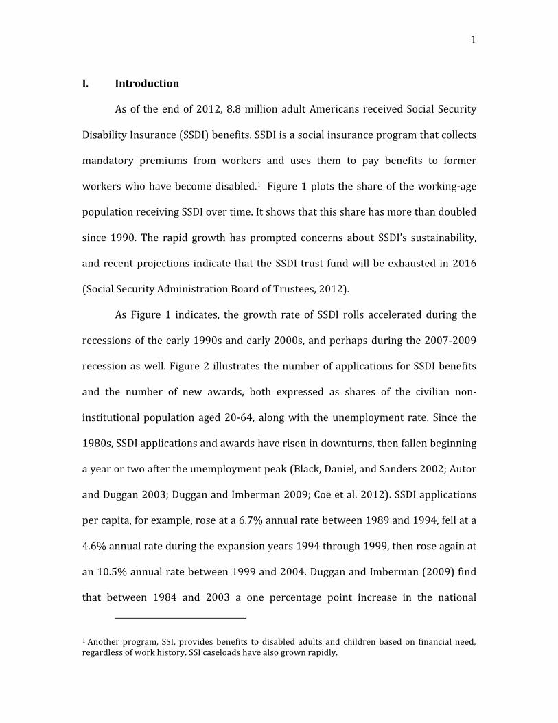
As Figure 1 indicates, the growth rate of SSDI rolls accelerated during the

recessions of the early 1990s and early 2000s, and perhaps during the 2007-2009

recession as well. Figure 2 illustrates the number of applications for SSDI benefits

and the number of new awards, both expressed as shares of the civilian non-

institutional population aged 20-64, along with the unemployment rate. Since the

1980s, SSDI applications and awards have risen in downturns, then fallen beginning

a year or two after the unemployment peak (Black, Daniel, and Sanders 2002; Autor

and Duggan 2003; Duggan and Imberman 2009; Coe et al. 2012). SSDI applications

per capita, for example, rose at a 6.7% annual rate between 1989 and 1994, fell at a

4.6% annual rate during the expansion years 1994 through 1999, then rose again at

an 10.5% annual rate between 1999 and 2004. Duggan and Imberman (2009) find

that between 1984 and 2003 a one percentage point increase in the national

1 Another program, SSI, provides benefits to disabled adults and children based on financial need, regardless of work history. SSI caseloads have also grown rapidly.

2

unemployment rate was associated with an increase of roughly 8-9 percent in the

number of applications filed for SSDI benefits. They conclude that nearly one

quarter of the rise in male SSDI participation between 1984 and 2003 can be

attributed to the recessions of the early 1990s and early 2000s.2 The cyclical

pattern is notably weaker after 2004 (von Wachter 2010). Applications declined at

only a 0.3% annual rate between 2004 and 2007, then grew at a 6.5% rate – far from

proportional to the magnitude of the Great Recession – between 2007 and 2011.3

Neither the older strongly countercyclical pattern nor its dampening in the

last decade are well understood. One explanation for countercyclical application

rates that would be generally consistent with the purposes of the SSDI program is

that employers’ willingness to hire (and make accommodations for) individuals with

moderately work-limiting disabilities may vary with the tightness of the labor

market. SSDI eligibility is restricted to individuals with functional impairments that

prevent them from performing their previous jobs or from adjusting to other types

of work. The worker’s age, education, and experience are considered in assessing his

or her suitability for alternative employment; as the jobs available to a worker with

a given profile likely depend on economic conditions, there may well be workers

who meet the medical eligibility criteria in bad economic times who would not be

considered to be sufficiently disabled were the labor market tighter.4

2 Other contributing factors include an aging population, increased female labor force participation (which increases women’s eligibility for SSDI benefits), more generous benefits, rising income inequality, and changes in the disability determination process (Duggan and Imberman, 2009). 3 The slow decline after the 2001 recession is consistent with other evidence that the subsequent expansion was relatively tepid. 4 In principle, medical eligibility does not depend on the availability of positions, but it seems likely that workers’ qualifications are in practice judged relative to labor demand. Joffe-Walt (2013)

3

Other potential explanations for the cyclical sensitivity of SSDI applications

attribute it to moral hazard. Consider a worker with a moderate health problem –

e.g., back pain – that makes work unpleasant but not impossible. In principle, this

worker should not be eligible for SSDI. But if he applies, a generous medical

examiner might award him benefits (Joffe-Walt 2013). His decision to apply will

depend in part on the generosity of SSDI benefits relative to the market wage that he

can command. If a recession reduces his market wage, he may be tipped over into

SSDI application (Autor and Duggan 2003; Black, Daniel, and Sanders 2002).

A related hypothesis is that workers use SSDI to insure employment losses

rather than wage declines. Displaced workers can generally claim unemployment

insurance (UI) benefits. But UI is time-limited and recessions are associated with

sharp increases in unemployment duration. Workers who exhaust their UI benefits

but who are still unable to find work may turn to SSDI for ongoing income support.

SSDI recipients tend to remain on the program, and out of the labor market,

until retirement (Autor and Duggan, 2006). As a result, any use of SSDI as a source

of extended unemployment benefits is extremely expensive. Indeed, a back-of-the-

envelope calculation, discussed below, suggests that savings from avoided SSDI

cases could plausibly finance a large share of the costs of extensions of UI benefits.

But little is known about the degree to which SSDI is in fact used in this way.

This paper uses data from the Great Recession and its aftermath to

investigate the relationship between UI exhaustion and SSDI applications. Our

describes a doctor who “believes he needs [to know individuals’ educational attainment] in disability cases because people who have only a high school education aren’t going to be able to get a sit-down job.”

4

analysis takes advantage of a great deal of variability of UI benefit durations during

the downturn. Potential benefits reached as high as 99 weeks in 2009, remained

high for several years, then declined substantially in 2012.5

At each point in this period there was substantial cross-sectional variation,,

due to vagaries of state law and to discontinuous triggers in federal programs. This

meant that workers laid off at roughly the same time were eligible for very different

UI durations depending on the location and exact timing of the layoff, and thus that

UI exhaustion rates varied substantially over time and across states. We use this

variation to identify the effect of UI exhaustion on SSDI usage, using time-series

analyses, state-by-month panels, event studies of weekly SSDI applications

surrounding UI extensions, and microdata on unemployed workers to isolate

different components of the variation in exhaustion timing.

Several recent papers have explored UI-DI interactions. Lindner and Nichols

(2012) use variation in benefit amounts and eligibility criteria to identify the causal

effect of UI participation on DI application decisions. The most relevant paper to the

current project is Rutledge (2012). With both aggregate state-month application

data and microdata from the Survey of Income and Program Participation (SIPP),

Rutledge examines the effect of UI benefit duration extensions on SSDI application

decisions and allowance rates. He focuses on the effect of a UI extension on the

behavior of those who were already claiming UI when the spell was announced.

5 Many models show that UI should be more generous during recessions (e.g., Landais, Michaillat, and Saez 2010), as moral hazard costs are relatively low and consumption smoothing benefits high when unemployment is elevated. A full discussion of optimal UI design is beyond the scope of this paper.

5

We extend Rutledge’s analysis in three important ways. First, our conceptual

model views UI extensions as a source of variation in the time to UI exhaustion

rather than as a direct determinant of SSDI applications, consistent with a

behavioral model in which individuals make decisions based on the benefits

available to them without regard to the legal labeling of those benefits. Second, our

empirical specifications are closely tied to this conceptual model, and are thus easily

interpretable in terms of the determinants of the underlying application decision.

This contrasts with Rutledge’s specifications, which are not closely aligned to a

behavioral model and focus on legal labeling – is an extension in effect or not? –

rather than on true incentives. Third, we introduce two new data sources that have

not been used previously to study UI-DI interactions. We have obtained access to

micro administrative SSA data that we use to tabulate weekly SSDI applications and

the corresponding award rates. We also use matched Current Population Survey

(CPS) samples to examine individual-level determinants of DI receipt.

II. A simple model of UI-DI interactions

Autor and Duggan (2003) model the choice between work and SSDI

application for marginally disabled workers. They show that some partially disabled

workers will stay in their existing jobs, but if displaced will prefer to exit the labor

force in order to receive DI benefits rather than to search for a new job at a lower

wage. Autor and Duggan interpret the cyclicality of SSDI applications as an

indication that there are meaningful numbers of workers of this type.

Autor and Duggan’s (2003) model does not incorporate unemployment

insurance. We extend their model to do so, drawing on Rothstein’s (2011) model of

6

UI and job search. In our model, a displaced worker can choose in each period

whether to search for work or to remain idle.6 Only search can lead to a new job,

while a DI application can be submitted only when in the idle state.

Searchers pay search costs cU and have a probability f of finding employment

each period. They can draw on up to N periods of unemployment benefits, worth bUI

per period. By contrast, workers out of the labor force do not pay search costs but

have probability 0 of finding employment and cannot draw UI benefits.

In a period that an individual is out of the labor force, he or she may apply for

DI benefits by paying an application cost cA. The probability that an application is

successful is p. We assume that DI eligibility decisions are perfectly correlated over

time, so that a worker who is rejected once will not later reapply. A worker whose

application is successful can draw a per-period benefit of bDI in any future period in

which he or she is out of the labor force, until such point as he or she is reemployed.

This basic setup gives rise to a dynamic decision problem with state variables

n {0, 1, …, N}, indexing the number of weeks of UI benefit entitlement remaining,

and A {0; -1; 1}, describing the worker’s DI entitlement. A=0 indicates a worker

who has not applied for DI benefits; A=-1 a worker who has applied but been

rejected; and A=1 a worker who has been awarded benefits. Letting indicate the

discount rate, u(y) the flow utility associated with per-period cash income y,7 and VE

the continuation value of a new job, the utility associated with job search is:

6 As UI benefits are paid only to workers with sufficient work histories who are involuntarily displaced, we focus on workers who prefer work to SSDI application, so will not voluntarily quit existing positions in order to apply for DI benefits. 7 We do not model saving or borrowing.

7

VU(n, A) = u(bUI) - cU + [f VE + (1-f) max{VU(n-1, A), VI(n-1,A)}] for n>0 and

VU(0, A) = u(0) - cU + [f VE + (1-f) max{VU(0, A), VI(0,A)],

where VI represents the value of idleness.8 This depends on the worker’s DI

application status. Those who have not yet applied for DI benefits or who have

applied but been rejected receive:

VI(n, A) = u(0) + max{VU(n, A), VI(n, A)}, for A {0; -1} and any n 0.

Those who have been approved for DI benefits receive:

VI(n, 1) = u(bDI) + max{VU(n, 1), VI(n, 1)}.

Finally, the utility of a worker who applies for DI benefits is:

VA(n, 0) = u(0) – cA + [ p max{VU(n, 1), VI(n, 1)} +

(1-p) max{ VU(n, -1), VI(n, -1)}].

Figure 3 shows how the worker’s policy choice varies with f and p, for a

particular set of other parameters. First, workers with high job-finding probabilities

search for work until they find jobs, even beyond the expiration of their UI benefits.

This is the upper area in the figure. Second, in the lower left, workers with low job-

finding probabilities but also low DI award probabilities search for work until their

UI benefits are exhausted, then exit the labor force without applying for DI.9 Third,

workers in the lower right region, with very high DI award probabilities but very

low job-finding chances, simply apply for DI immediately after displacement,

8 Because we assume that parameters are stationary, it can be shown that any worker who chooses search with A=0 and n≠1 will also choose search the following period. The max operators in the VU

expressions are thus relevant only for n=1. 9 With the parameter values used, job search is worthwhile for the duration of UI benefits even if the job-finding probability is zero, as the UI benefit is larger than the search cost. If bUI is low enough relative to cU, however, a policy of exiting the labor force immediately after job loss becomes optimal for low-f, low-p workers.

8

without ever looking for work. Finally, workers with somewhat lower DI award

chances and/or somewhat higher job-finding probabilities search for work until

their UI benefits are exhausted, then apply for DI benefits.

It is this last type of worker that could produce a causal effect of UI benefit

durations on DI applications, as these workers can be deterred from applying for DI

by a UI extension. For some, this is temporary – they will still be jobless at the end of

the extended benefits, and will apply to DI then. But others will find jobs during the

extended search period, and thus may be permanently diverted from the DI

program.

This diversion could be substantial. To see this, suppose that {f, p} have a

uniform distribution on [0, 0.1] X [0, 1] among displaced workers and that other

parameters are as in Figure 3. Then 17% of workers, and 35% of those who exhaust

26 periods of UI benefits, are of the UI-before-DI type. When UI benefits last for 26

weeks, UI-before-DI workers comprise 83% of DI applicants and 79% of DI

awardees. The average UI-before-DI DI applicant has a per-period job-finding rate of

1.5%. Thus, some would find jobs if given longer UI benefit durations during which

to search. With our parameters, a 26-period extension of UI benefits (to a total of 52

periods) would permit just under one-third of the UI-before-DI workers who would

otherwise apply for DI to instead find new jobs before their benefits run out. This

would reduce steady-state DI applications and awards by a bit over one-quarter,

while increasing UI payments by about 40%.

An effect of this magnitude would be enormously important. Because

individuals awarded DI benefits tend to draw them until retirement, the present

9

value of a single DI award is around $300,000. By comparison, weekly UI payments

average around $300. Thus, the parameters used in Figure 3 and a uniform

distribution of {f, p} imply that DI savings from a 26-week UI extension would

amount to over three times the on-budget cost of that extension. In other words, a

UI extension would be self-financing even if the effect on steady-state DI awards

were only one-third as large as in this simple simulation.

But the parameters used are just approximations, and the assumption of a

uniform {f, p} distribution is entirely unsupported. It seems more likely, for

example, that f and p are negatively correlated. This would increase the share of UI-

before-DI workers, though perhaps also reduce their average job-finding rates. Non-

uniformity of the two marginal distributions could offset any such effect. The effect

of UI benefit duration on DI applications is thus an empirical question.

III. Data and DI trends

We rely on three data sources to measure trends in SSDI application and

receipt. First, we use publicly available tabulations from the Social Security

Administration (SSA) of SSDI, SSI, or SSDI/SSI applications at the state-by-month

level between August 2004 and December 2012.

Second, we obtained access to SSA’s Disability Research File, a restricted-

access micro data file covering the years 2008-2010 and containing observations on

individual SSDI applications linked to application outcomes. We use these data to

construct a state-by-week panel of application counts. We also calculate eventual

award rates for each weekly application ‘cohort’, using information on awards over

the remaining horizon in the sample.

10

Third, we use the Annual Social and Economic Supplement (ASEC)

supplement to the Current Population Survey (CPS), administered in the spring of

each year.10 Respondents are asked about their income from various sources in the

previous calendar year. Those who report income from Social Security are asked to

list reasons for this. We measure SSDI receipt as the presence of positive Social

Security income for someone who names “disability” as one of the reasons.

Figure 4 shows trends in the number of disabled worker SSDI recipients from

the published SSA data, along with two series computed from the CPS ASEC. One

series counts all individuals aged 16 and over who report Social Security disability

income. The second excludes those over age 66 (67 after 2009, reflecting an

increase in the Full Retirement Age), as disabled individuals above this age receive

retirement payments rather than SSDI. The former series matches the

administrative records reasonably well, though shows a somewhat flatter trajectory.

The latter is notably lower, suggesting both that many recipients continue believing

they are receiving disability benefits even after they are formally converted to the

retirement program and that the CPS survey misses some true SSDI recipients.

In the analysis below, we identify unemployed workers, aged 20-64, in the

basic monthly CPS survey and ask whether the expiration of their UI benefits early

in calendar year y is associated with a higher probability of receiving SSDI income in

that year. This is made possible by the rotating panel design of the CPS, which

means that just under half of the respondents in the y+1 ASEC file can be matched to

10 The ASEC is often known as the “March CPS.” It borrows the March sample from the regular monthly CPS survey, supplementing this with portions of the February, April, and November (of the previous year) monthly CPS samples.

11

basic CPS interviews in February, March, or April of year y, or in November of year

y-1. The CPS is an address-based sample, so matches are only possible for

individuals who do not move between surveys. We are able to match around 95% of

ASEC respondents to one of the surrounding monthly surveys. Merges between

year-y and year-y+1 ASECs are more difficult, with match rates around 75%.11

In the basic CPS survey, unemployed workers are asked the reason for their

unemployment (e.g., layoff vs. voluntary quit) and the number of weeks that they

have been unemployed. We use the former to proxy for UI eligibility and the latter to

assign each unemployed individual to the date of displacement. We then use a

database of state UI rules, discussed in Section IV, to assign the date that the worker

would have exhausted his UI benefits if he was eligible for full benefits and if he

drew benefits continuously from the date of displacement until exhaustion.

IV. UI during the Great Recession and its aftermath

A. Extended UI Programs

Workers displaced from covered employment with sufficient work histories

are generally eligible for up to 26 weeks of regular unemployment insurance

benefits. But at times during the last few years, workers who have exhausted their

regular benefits might have drawn as many as 53 additional weeks of Emergency

Unemployment Compensation (EUC) and as many as 20 more weeks of Extended

Benefits (EB), bringing the total as high as 99 weeks. There has been substantial

11 This excludes observations that should not match due to the structure of the survey (e.g., those in their second sample rotation in year y). About 1% of monthly-to-ASEC matches and 6-8% of ASEC-to-ASEC matches show discrepancies in age, race, gender, or education. Discrepant observations are discarded.

12

variation in this maximum over time and across states, resulting from differences in

state policies, from changing Federal law, and from “triggers” that conditioned both

EUC and EB benefits on state economic conditions.

The EUC program was first authorized in June 2008.12 It initially provided 13

weeks of federally-financed benefits to supplement the regular 26 weeks. At the

time, the recession was expected to be relatively brief, and EUC was set to expire in

March 2009. As the downturn proved to be deeper and longer lasting than initially

expected, EUC was gradually expanded. In November 2008, EUC benefits were

extended to 33 weeks in states with unemployment rates above 6 percent and to 20

weeks elsewhere. They were extended again in November 2009, to 34 weeks in low

unemployment states and 53 weeks in high unemployment states.

EUC complemented a preexisting program, EB, which was designed to

provide supplemental weeks of benefits in times of economic distress. States choose

whether to participate in EB and, if they participate, select from a menu of possible

triggers that will activate EB benefits. Activation provides 13 weeks of EB benefits

(on top of the regular and EUC eligibility), or 20 weeks in states that have adopted a

more generous trigger and that have unemployment rates above 8%. The first state

to become eligible for EB benefits in the Great Recession was Alaska, in June 2008;

five additional participating states became eligible by January 2009.

The cost of EB benefits is ordinarily split between the state and the Federal

government, but the American Recovery and Reinvestment Act of 2009 (ARRA; also

12 It resembled other, similar temporary programs created in past recessions. The discussion here draws on Rothstein (2011) and Fujita (2010).

13

known as the Recovery Act) provided for full Federal funding. After this, a number

of states passed legislation to adopt the program or to liberalize their triggers. By

May 2009, recipients in 27 states could receive EB benefits, and 11 of these offered

20 weeks of benefits. Eligibility continued to expand, with between 36 and 39 states

paying EB benefits through most of late 2009, 2010, and early 2011.

Both EUC and EB benefits were gradually rolled back starting in mid 2011.

The EB rollback was largely automatic, due to rules that condition eligibility on not

just a high but also a rising unemployment rate. During the aftermath of the

recession, unemployment remained high but slowly declined. The number of states

paying EB benefits fell through the second half of 2011 and the first half of 2012. By

July 2012, only Idaho was still paying benefits; it triggered off in early August.

The major rollback of EUC came in February 2012, when legislation made

several changes. First, EUC durations were cut by 6 to 14 weeks, depending on the

state unemployment rate (though states with rates between 7 and 8.5% or above

9% were unaffected). Second, further cuts were scheduled for September 2012.

Third, additional weeks of EUC benefits were provided to high-unemployment

states that did not qualify for (or did not participate in) the EB program. This

provision provided ten extra weeks in March, April, and May of 2012; none in June,

July, and August; and four extra weeks from September onward.

On top of the basic story of haphazard expansion and rollback, additional

variation in EUC durations arose from the temporary nature of the program. The

program was initially set to expire in March 2009. In February 2009, the ARRA

14

extended it through December of that year.13 During 2010, Congress then extended

it several times for only a few months each: From December 2009 to February 2010,

then to April, to June, and to November 2010. Several of these extensions were

retroactive, authorized only after the program had already expired. The first

expiration lasted only a few days, but two others lasted for about two weeks each

and in June and July 2010 the program was allowed to expire for a full seven weeks.

A longer-term extension finally took effect in December 2010.

Figure 5 shows the average, minimum, and maximum number of weeks of

benefits available over time through the recession, combining the regular, EUC, and

EB programs. This figure is made from a database of UI availability at the state-by-

week level, constructed by Rothstein (2011) but updated here to the end of 2012.

Maximum benefit durations reached 99 weeks from late 2009 through mid 2012,

and the average state was close to the maximum through much of this period. States

began to fall away from the maximum during early 2012.

The three expirations of the EUC program in 2010 are quite prominent in the

figure, as durations fall dramatically in each. However, the sharp declines indicated

likely overstate the changes experienced by individual recipients. EUC benefits are

divided into tiers – at its peak, the 53 weeks of maximum EUC benefits were divided

into four tiers of 20, 14, 13, and 6 weeks, respectively. When the program expired

recipients were permitted to continue to draw benefits until they exhausted their

current tier but could not begin a new tier, while people who exhausted their

13 ARRA also made UI benefits more generous in a number of ways, including by providing a $25/week supplement to UI benefits and by exempting the first $2,400 of benefits from income taxes. Both provisions were temporary.

15

regular benefits were not permitted to enter the EUC program.14 This tended to

smooth over the expirations, limiting the disruption produced. But the degree of

smoothing depended importantly on the exact date of job loss, as this determined

the worker’s position in the tier structure at the time of EUC expiration.

Each eventual reauthorization provided for the retroactive payment of

benefits to individuals who would have received EUC but for the temporary

exhaustion. The long-term unemployed are unlikely to have substantial liquid

savings or easy access to credit (Gruber 1997), however, so many may have felt

serious financial crunches during the expirations.

B. Modeling UI Exhaustion

The complex history of EUC and EB created a great deal of variation in the

duration of UI benefits and thus in the timing of UI exhaustion. Unfortunately, while

the Employment and Training Administration (ETA) compiles weekly counts of

initial UI claims, no comparable data series is available for exhaustions. We take two

approaches to approximating the number of exhaustions.

Our first exhaustion series is constructed from state-by-month level ETA data

on the numbers of first payments and final payments in each program and EUC tier.

For each state in each month, we compute the number of final payments in any

program or tier minus the number of first payments in the EUC tiers or EB. This

closely approximates exhaustion, but there are three sources of slippage. First, this

14 100% federal financing of EB expired each time the EUC program did. Many states conditioned their EB participation on continued federal funding, and cut off EB benefits within a week or two of the June 2010 expiration. EB benefits lost during this period were in general not paid retroactively.

16

method incorrectly counts as exhaustions individuals who found new jobs or

abandoned their job searches upon the expiration of a particular tier or program but

who had more benefits available on another tier or program. Second, when

individuals receive their final payments from one program or tier in the last week of

a calendar month, the initial payment on the next program or tier appears in the

next month’s data. This creates excess volatility in measured exhaustions. Third,

when EUC benefits were expanded –when new tiers were introduced, when the

program was retroactively reauthorized, or when a state triggered on to new

benefits – many people received first payments who had not received final

payments in the previous week. We estimate negative numbers of exhaustions at

these times. These moments are quite useful for identification of UI effects, however,

as they represent periods when UI exhaustions were low or zero. We present

analyses below that zero in on DI application dynamics surrounding UI extensions.

The solid line in Figure 6 shows the estimated number of UI exhaustions each

month, using this method. Exhaustions were fairly stable, at around 210,000 per

month, through early 2008. Measured exhaustions turned sharply negative in July

and August of 2008, following the creation of EUC. They then became volatile,

bouncing around a lower mean through the rest of 2008 and 2009 with two dips

into negative terrain following EUC expansions in February 2009 and December

2009-January 2010. Exhaustions spiked enormously during the temporary EUC

expiration in June 2010, only to turn negative again in August 2010 after the

program was reauthorized. Following this episode, the series has bounced around a

level similar to that seen before the recession but higher than the 2008-9 average.

17

Although the spikes and negative values represent measurement problems,

the broad patterns – declines in exhaustions in 2009-10 followed by an increase in

2011-12 – correspond to real dynamics. In 2009-10, benefit durations were quite

long, and many recipients found jobs or exited the labor force before they exhausted

benefits, while the cohorts that were approaching exhaustion were primarily those

that had lost their jobs before the recession so were not particularly large. In 2011-

12, durations remained long, but the large 2009 cohorts were exhausting their

benefits, offsetting the effect of extended durations on the exhaustion rate.

We simulate an alternative UI exhaustion measure to use as a check on the

administrative data. We begin with weekly data on initial claims for regular UI

benefits by state. We then use our state-by-week database of UI availability to

identify the week that each entering UI cohort would have exhausted its benefits,

assuming eligibility for full benefits and continuous claiming. Next, we estimate the

probability that an individual entering unemployment in each week would have

survived in that status (rather than becoming reemployed or exiting the labor force)

until the expiration of benefits. The survival probabilities are described in the

appendix; they are based on estimated average UI exit hazards that are allowed to

vary smoothly over time and discretely with unemployment duration. By

multiplying the size of the entering cohort by the survival probability, we estimate

the number of UI exhaustions produced by the cohort when its benefits end, then

18

aggregate across all cohorts that exhausted their benefits in each month to construct

an estimated exhaustion series.15

Two series obtained via this method are plotted in Figure 6, corresponding to

different definitions of “exhaustion.” The first series, plotted as a dotted line, judges

an individual to have exhausted her benefits in the first week that she did not

receive an on-time benefit payment, even if she was later paid retroactively for that

week. This series mirrors the general trends in the administrative measure, but

shows zero exhaustions rather than negative numbers in months following EUC

introduction and expansions. It also, however, shows an enormous spike in June

2010, when EUC was allowed to expire. (This data point is censored in the graph to

control the overall scale; in fact, the series shows nearly 2.5 million exhaustions that

month.) It is unclear whether this accurately reflects the expirations that are

relevant to SSDI application decisions. If recipients were confident that Congress

would eventually reauthorize the program retroactive to its expiration, and if they

had access to sufficient credit to borrow against their eventual benefits, this spike

dramatically overstates the number of true exhaustions.

Our second simulated exhaustion series, graphed as a dashed line, counts

individuals to exhaust their benefits only when they receive their final payments

under any program, ignoring temporary breaks that are repaid retroactively. This

does not show a pronounced spike in June 2010 but does a better job of mirroring

15 There is an additional adjustment to account for the fact that not all claims for UI benefits lead to actual benefit payments.

19

the patterns in the administrative data in 2011. We use this as our preferred

exhaustion series in the analyses below.

Our simulated final exhaustion series explains 9% of the time series variation

in the administrative data measure (and 21% when June-August 2010 are

excluded). There is substantial across-state variation concealed behind the

aggregate time series shown in Figure 6. New York, for example, saw essentially

zero exhaustions in 2008 and 2009, while Virginia saw as many or more

exhaustions each month in 2008 as before the recession. We exploit this variation in

many of the estimates below. A natural concern is that the state-by-month

exhaustion measures may be particularly noisy at the state-by-month level.

However, they do seem to have substantial signal: The elasticity of the

administrative data exhaustion measure with respect to simulated final exhaustions,

controlling for state and month effects, is 0.24, with a standard error of 0.03. 16

When we exclude the June – August 2010 period, the elasticity rises to 0.28.

V. Analyses of UI-DI interactions using aggregate data

In this section, we present time-series, state-by-month panel data, and state-

by-week event studies of the relationship between UI exhaustions and DI

applications as well as award rates. Recall that the model in section II suggested that

some marginally disabled UI recipients might be induced to apply for SSDI benefits

by the impending or actual exhaustion of their UI benefits. This would imply a

16 As an alternative to modeling log exhaustions – there are many zeros at the state-by-month level –we normalize monthly exhaustions in each state by the average number of monthly exhaustions in the state in 2005-2007. The elasticity reported in the text is based on the normalized series, which we use for all further analyses.

20

positive correlation between UI exhaustions and SSDI applications. Insofar as the

marginal DI applicants are less likely to be awarded benefits, it should also produce

a negative correlation between UI exhaustions and SSDI acceptance rates.

A. Time Series Analyses

We begin by overlaying our simulated final UI exhaustion series with the

number of monthly SSDI applications, in Figure 7. There is little sign in this graph of

a positive relationship between UI exhaustions and DI applications. Though UI

exhaustions fell to well under half of their usual rate through most of 2009, DI

applications rose by about 20% in late 2008 and early 2009.17 UI exhaustions

returned to close to their pre-crisis level in late 2010; DI applications plateaued

around that time and have remained roughly stable since.

Table 1 presents time-series analyses of the log of seasonally-adjusted

aggregate monthly DI applications. The first column includes only the simulated

number of final UI exhaustions in the month, measured as a share of their average

level during calendar years 2005-2007. The coefficient is negative, the opposite of

the expected sign if UI exhaustions lead to DI applications, but is insignificant and

small. Column 2 adds a quadratic time trend, while column 3 adds a control for the

unemployment rate. The unemployment rate coefficient is positive and quite

precisely estimated, indicating that a one percentage point increase in

unemployment is associated with a 3.9% increase in DI applications. The UI

17 We seasonally adjust the DI series using state-level regressions of log monthly applications on calendar month dummies, controlling for quadratic time trends, an indicator for observations since February 2009, and the number of weeks in the month. We then sum adjusted state applications to form a national series.

21

exhaustion coefficient becomes positive and marginally significant (t=2.01) when

the unemployment rate is controlled, but is quite small: A doubling of UI

exhaustions is associated with only a 1.5% increase in DI applications.

Column 4 adds several controls: the number of initial UI claims, seen as

proxies for economic conditions; an indicator for June-August 2010 observations,

when the expiration of EUC makes it difficult to measure perceived UI exhaustions;

and an indicator for the period after February 2009. These have essentially no effect

on the coefficient of interest.

Column 5 adds the averages of three leads and three lags of UI exhaustions.

Each of these might capture true effects of UI exhaustions on DI applications, which

need not be exactly contemporaneous. But there is little indication that the

contemporaneous specification misses an important part of the response – neither

the lag nor the lead is significant, the contemporaneous effect is basically

unchanged, and the point estimate of the cumulative effect is almost exactly zero.

Columns 6-8 explore alternative measures of UI exhaustions. In column 6 we

use the simulated series for initial exhaustions (the dotted line from Figure 6), while

in column 7 we use the exhaustion series computed from administrative records on

EUC and EB initial and final payments (the solid line from Figure 6). Neither of these

series indicates any relationship between exhaustions and DI applications. Finally,

in column 8 we replace the counts of exhaustions with an indicator for the four

months in which our simulations suggest that there were zero UI exhaustions,

immediately following the introduction of the EUC program in mid 2008 and its

22

expansion in late 2009. This specification indicates that DI applications fell about

1.9% in these months, implying similar responsiveness to that found in columns 3-5.

All told, the specifications in Table 1 indicate that any effect of UI exhaustions

on DI applications is quite small and sensitive to the way that exhaustions are

measured. By contrast, there is a robust and large relationship between the

unemployment rate and DI applications that does not appear to reflect an

association between overall unemployment and UI exhaustions.

B. Panel Data Analyses

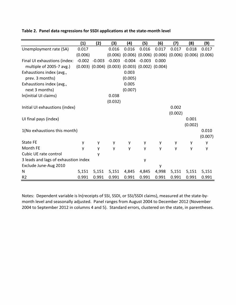
We next turn to panel data analyses of log monthly DI applications at the

state level, in Table 2. These allow us to control for other factors that influence the

time pattern of DI applications, identifying the exhaustion effect from differences

across states in exhaustion trends. There is substantial variation in these trends,

driven in part by the timing of layoffs and in part by variation in UI availability.

Column 1 begins with a simple specification that includes state and month

fixed effects, the unemployment rate, and the state-level index of final UI

exhaustions. The unemployment rate coefficient is positive and significant, though

somewhat smaller than in Table 1. The UI exhaustion coefficient is almost exactly

zero. Moreover, it is extremely precisely estimated, with a standard error less than

half of those in Table 1, and we can thus rule out elasticities of DI applications with

respect to UI exhaustions larger than 0.005.

Columns 2 and 3 explore alternative controls for economic conditions. These

have little effect on the results. Column 4 includes lags and leads of the exhaustion

index. These are both insignificant, and the point estimates indicate a cumulative

23

elasticity of DI applications with respect to exhaustions of only 0.018. In column 5,

we include each of the three leads and three lags of the exhaustion series separately.

Point estimates (not shown) indicate a cumulative elasticity of 0.004, with negative

coefficients for the contemporaneous and immediate leads and lags and positive

coefficients on the longer leads and lags. This is the opposite of the pattern that one

would expect from a causal effect of anticipated or recent past UI exhaustion.

Column 6 excludes the June-August 2010 observations, when UI exhaustions

are difficult to define precisely. This has little effect.

There are two sources of variation in our simulated UI exhaustion measure:

Variation in the size of entering UI cohorts (i.e., in the number of new claimants) and

variation in the duration of UI benefits. We have also created alternative simulations

that hold the cohort size constant, so that benefit durations are the only source of

variation. When we use these measures as instruments for the original measures,

results are quite similar to those seen in Table 2, and the upper bounds of the

confidence intervals are if anything smaller.

Finally, columns 7-9 of Table 2 explore our alternative UI exhaustion series.

They indicate slightly more positive effects, though they still rule out elasticities

larger than 0.006. Moreover, column 9 indicates that DI applications rise in months

when new UI extensions take effect, and the confidence interval rules out declines

larger than 0.4%. We return to this investigation below.

The published data cannot be used to examine award rates, as awards are

reported for the month of final adjudication rather than for the month of initial

application. As an alternative, we use the SSA microdata to examine the acceptance

24

rate for SSDI applications filed in each state in each month in 2008, 2009, and

2010.18 Table 3 presents results parallel to those in Columns 1, 4, 7 and 8of Table 2.

Each of the specifications shows an insignificant, near zero relationship between DI

acceptance rates and UI exhaustions. The only exception is in Column 2, where

average exhaustions over the previous three months are significantly but positively

related to the acceptance rate, the opposite of the expected sign.

Taken together, the panel data analyses in Tables 2 and 3 offer no sign that

DI applications or awards respond to UI exhaustions. We can always rule out

application elasticities larger than 0.02, and most specifications rule out elasticities

one-quarter this size.

At this point, it is worth considering how large an effect would need to be to

be quantitatively important. One way to approach this is to compare the empirical

estimates to the elasticities implied by the toy model in Section II. In that model, a

doubling of UI durations reduced steady-state UI exhaustions by about half and

steady-state DI applications by a quarter. (The short-run effects would be much

larger.) The estimates in Tables 2 and 3, then – if they can be interpreted as causal –

imply much, much smaller UI exhaustion effects.

Another approach is to compare the cost of UI extensions to the resulting DI

savings. As noted earlier, the present value of a DI award is around $300,000, while

UI benefits cost around $300 per week. Thus, if extending UI benefits by one week

18 Appendix Table A.1 reports application analyses conducted using only the period covered by the microdata. Results are similar to those in Table 2.

25

diverts even one in one thousand recipients from going on DI, the DI savings would

pay the entire cost of the UI extension.

However, the first-order effect of a UI extension is likely to be to merely delay

DI applications rather than to permanently displace them. Rothstein (2011)

estimates that the long-term unemployed had monthly job-finding rates around 10

percent through 2009 and 2010. If we suppose that marginal DI applicants have

similar job-finding rates to this and if we assume a DI award rate of one-third,

roughly matching the recent average, then a four-week UI extension would be fully

financed through DI savings if it deterred 120 DI applications per 1,000 potential UI

exhaustees. This almost certainly understates the needed amount of deterrence, as

marginal DI applicants are probably less employable than the average long-term UI

recipient and likely have lower award rates than average DI applicants.

Recall that the estimates in Table 2 always ruled out elasticities of DI

applications with respect to UI exhaustions larger than 0.02. DI applications are of

the same rough order of magnitude as UI exhaustions, so this implies a reduction of

not more than 20 DI applications per 1000 UI exhaustees whose benefits are

extended, well below the break-even point. Moreover, this is based on the upper

limit of the confidence intervals; point estimates imply zero or even negative effects.

C. Event Analyses

We next use our administrative micro data to conduct event studies of

weekly DI applications in the periods immediately surrounding extensions of UI

benefits. These have several potential advantages over the analyses above. First,

they do not require us to rely on our imperfect UI exhaustion measures; we can be

26

confident that UI exhaustions declined drastically following new benefit extensions.

Second, the event study framework allows us to more flexibly examine the time

pattern of any application responses to UI extensions. Third, the only lever by which

UI exhaustion might be manipulated is the extension of UI benefits, so reduced-form

event studies of UI extensions are directly informative about policy effects.19

In implementing the event study, we face two challenges. First, we cannot

identify the individuals at risk of UI exhaustion in DI data. Thus, as above, we

examine the effect of UI extensions on aggregate DI applications. Second, many

states saw repeated UI extensions over relatively short periods in 2008 and 2009,

which makes it difficult to distinguish long-run effects of one extension from short-

run effects of the next. Thus, while a full assessment of the impact of UI extensions

would consider the cumulated net effect, starting from the date that the extension is

first anticipated and extending until well after the last cohort affected by the

extension exhausts its UI benefits, we focus on shorter-run impacts and on

extensions that do not closely overlap.

We define event dates as the weeks on which UI extensions came into effect,

as reported in “Trigger Notices” published by the U.S. Department of Labor. We

estimate specifications of the form:

∑

19 One can interpret the event study estimates as the ‘reduced forms’ corresponding to 2SLS estimators in which UI benefit extensions are used as instruments for UI exhaustion. We discussed 2SLS estimates like this above.

27

where represents the log of the number of SSDI applications filed in state s

in week t. and are time and state fixed effects, respectively. measures the

difference from the national weekly trend k weeks after (or |k| weeks before, when

k<0) the event date, and N is the number of weeks the extension was in place. Xst

contains polynomials of degree three for the state-level unemployment rate as well

as the state-level insured unemployment rate. Note that the state-level

unemployment rate is only available at the monthly frequency.

Figure 8 shows the coefficients for the four weeks immediately preceding

and following an extension in UI durations. Panels A and B show estimates for log

weekly SSDI applications, the first using both short extensions (often providing only

6 weeks of additional benefits) and the second using only extensions of 13 weeks or

more, while Panels C and D show estimates for award rates. The corresponding

coefficients, standard errors, and p-values are shown in Appendix Table A.2.

We begin with the results for DI applications, in Panels A and B. These show

an uptake in SSDI applications prior to UI extensions, relative to the average 5

weeks or more before the extension. This is robust to a range of alternative

specifications. We would not expect much of an anticipation effect, as many

extensions were not easily predicted; moreover, this is the opposite of the expected

sign. We are concerned that the effect may reflect uncontrolled variation in

economic conditions that leads both to “triggering” UI extensions and to increases in

SSDI applications. However, the effect disappears when we restrict attention to non-

28

overlapping extensions, shown as dashed lines.20 We therefore put more emphasis

on these results.

The solid lines drop slightly after extensions take effect, both in Panel A and

Panel B. We can reject the hypothesis that the effects during the week of the

extension and in the four weeks after the extension are jointly zero, and several of

the individual coefficients are statistically significantly different from the pre-

extension average. The estimates based on non-overlapping extensions, however,

show no drop in DI applications (save for a small, statistically insignificant dip in the

week of the extension).

Overall, the event study paints a mixed picture of the effect of UI extensions

on SSDI application rates. On the one hand, the results that include all extensions

suggest that there might be modest negative initial effects on SSDI applications,

averaging around 2.5 percent (relative to the immediate pre-extension levels) over

weeks 0 to 4. As exhaustion rates fall to zero during this period, this is somewhat

larger than, though broadly consistent with, the upper bound of the confidence

intervals we obtained in the panel data analysis above. It is still well below the

break-even point. On the other hand, these effects are absent for non-overlapping

extensions, which are both more clearly exogenous and easier to interpret as policy

experiments. Overlapping extensions might have no immediate effect on UI

exhaustions if prior extensions have already ensured zero exhaustions in the short

term, so it is surprising that these extensions appear to drive the effects we see.

20 To be precise, we define an overlapping extension as an extension that follows an earlier x week extension by less than x weeks, for any x.

29

Panels C and D of Figure 8 repeat the event study analysis for SSDI award

rates, computed as the share of applications that lead to eventual awards.21 There is

no sign of a systematic effect of UI extensions on award rates along any dimension.

An advantage of the individual level SSA data is that they permit us to

disaggregate the analyses by demographic groups. Figure 9 shows event-study

estimates for three major age groups, focusing on large, non-overlapping extensions.

Estimates show no sign of systematic effects. Negative post-extension coefficients

are nearly all for the youngest age group, which contributes the smallest share of DI

applications, and are never significant (individually or jointly).22 This confirms our

interpretation of the event studies as consistent with the panel data analyses in

indicating little overall effect of UI extensions on SSDI applications. The lower panel

of Figure 2 shows the effect on the acceptance rate by age group. Again, estimates

are noisier for the youngest group but close to zero for the middle and older groups.

VII. Analysis of UI-DI interactions using Current Population Survey microdata

All of the above analyses are ecological, aiming to tie trends in aggregate DI

applications and awards to trends in UI exhaustion. As a final exercise we turn to

our merged CPS microdata to examine the individual-level relationship between UI

exhaustion and DI receipt.

Table 4 presents summary statistics for the merged CPS sample, pooling data

for calendar years 2005 – 2011 (with ASEC observations from the 2006-2012

21 Our data capture only awards made in 2010 and earlier. As a result, there is some censoring in our data. This should be captured by the calendar time effects in our event-study specification. 22 The only statistically significant post-extension coefficient is for the acceptance rate of applications filed by 50-64 year olds two weeks after an extension, and this is positive.

30

surveys). We restrict the sample throughout to individuals aged 20-64 (in the base

month survey), and we those whose unemployment spells started in 2003 or earlier.

The first column presents statistics for the full sample (N= 240,163). 75% are

employed at the initial monthly survey (generally in March of year y, though some

are from February or April, or from November of year y-1), 5% are unemployed, and

21% are out of the labor force. The subsample of unemployed workers is described

in column 2, while column 3 summarizes job losers. Unfortunately, we cannot

measure UI receipt directly. However, the reason for unemployment appears to be

an adequate proxy: Of those who were unemployed at the initial monthly survey

and said that they had been involuntarily displaced, 40% report on the following

March’s ASEC survey having positive UI income for the year. This compares to only

9% of those who say that they had voluntarily left their previous job or were new

entrants or reentrants to the labor force.

Column 4 presents statistics for UI-eligible workers who would have

exhausted their benefits before the end of the year in which they were initially

observed, had they remained unemployed for that long. (Of course, not all workers

reached that point – some presumably were reemployed before exhausting their

benefits. But we cannot measure these transitions.) All UI recipients in 2005-2007

are in this category, as the base surveys were completed by April and UI benefits

lasted only 26 weeks in those years. In later years, only workers who had already

been unemployed for some time by the initial survey were at risk of exhausting their

UI benefits within the calendar year.

31

Of the UI eligible workers in the base month survey, 57% would have

exhausted their benefits by the end of the calendar year, and 37% would have

exhausted them by the midpoint of the year. The potential exhaustees closely

resemble the overall pool of UI eligible workers in their demographic

characteristics. The average time of expiration is in early March of year y.

The final rows of the table show the share of individuals who report in the

year-y+1 ASEC survey having received SSDI income during year y. This is 3.2% for

the full sample, but over half of these also reported having SSDI income in year y-1.

We exclude them from our analysis of the effect of UI expiration. Only 1.4% of

individuals who did not have SSDI income in year y-1 had it in year y. Unemployed

workers and particularly job losers have below-average SSDI receipt rates. Among

UI recipients, those who would have exhausted their benefits before the end of year

y have somewhat higher SSDI recipiency rates than do those whose benefits would

have continued beyond the end of the year.

Table 5 presents our analysis of UI expiration and DI receipt in the matched

CPS-ASEC sample. We estimate specifications of the form:

DIisy = logit(URsy β + LFisy γ + Xisy δ + Disy θ + κs + πy),

where DIisy is an indicator for receipt of SSDI income by individual i in state s in year

y (as reported on the y+1 ASEC survey); URsy is the unemployment rate in state s in

year y; LFisy is a vector of measures of the individual’s labor force status, including

dummies for unemployment and NILF (employment is the excluded category) and

measures of unemployment duration; and Xisy is a measure of UI exhaustion before

the end of year t. Disy is a vector of demographic controls – dummies for ages 40-49,

32

50-54, 55-59, and 60-64, with 20-39 the excluded category; a linear age control; and

a gender indicator. κs and πy are fixed effects for states and years, respectively.

Column 1 presents a specification that includes only the demographic

controls, state and year FEs, and the state unemployment rate. The latter enters

with a negative coefficient, though it is insignificant and the implied effect is very

small. Column 2 adds indicators for four labor force statuses at the base survey:

Unemployed due to job loss, unemployed due to voluntary quit or to labor market

entry or reentry, non-participation in the labor force due to disability, and non-

participation for other reasons. (The excluded category is employment.) Those who

are not employed at the base survey have substantially higher probabilities of

receiving SSDI than are the base-survey employed. Those out of the labor force have

higher probabilities than the unemployed, particularly so for those who attribute

their non-participation to disability.

Logit coefficients can be difficult to interpret, particularly when positive

outcomes are rare. We thus use the coefficients to predict how much lower the SSDI

receipt rate would be if these individuals had instead been employed. These

estimates, reported in the bottom rows of Table 5, indicate that unemployment

accounts for two-thirds of the observed 0.97 percentage point rate of DI receipt

among the unemployed.

Column 4 adds the unemployment duration (measured as of the end of the

calendar year, assuming that the initial unemployment spell lasts until then), alone

and interacted with UI eligibility. Those who are employed or out of the labor force

at the base survey are assigned durations of 0. The longer-term unemployed are

33

more likely to receive SSDI income than are those unemployed for shorter periods,

particularly among job-losers.

Column 5 adds two UI expiration measures. The first is a continuous measure

of time (in years) from the date of UI expiration to the end of the focal year. Those

whose benefits continued beyond the end of the focal year are coded as zeros. The

second measure is an indicator for an expiration before June 30. Because DI

applications take several months to process, an individual whose UI benefits expired

late in the year and who applied for SSDI immediately thereafter would be unlikely

to receive DI income in that calendar year. Those whose applications were filed

early in the year, however, should have reasonable probabilities of receiving DI

income by the end of the year. Thus, if UI expirations lead in relatively short order to

DI applications and if some of those applications are successful, both variables

should be positively associated with DI receipt.23

The estimates do not indicate this. Expiration before June 30 has a positive

coefficient while the continuous time since UI expiration is negative, but they are

not individually or jointly (p=0.84) significant, and both are quite small. The

coefficients imply that delaying all UI exhaustions beyond the end of the focal year

would reduce DI receipt among the unemployed by only 0.01 percentage points.

This result is unaffected by the addition of quadratic and cubic terms in the state

unemployment rate, in column 6.

23 Implicit in this parameterization is an assumption that the probability of DI receipt rises with the time elapsed since the DI application, perhaps particularly quickly around 6 months after the initial application.

34

Column 7 restricts the sample to the unemployed and column 8 to job losers.

These dramatically reduce the sample size, reducing precision. Point estimates

indicate somewhat larger exhaustion effects – in the final column, they suggest that

expiration of UI benefits raises the probability of DI receipt among the UI-eligible

unemployed by 0.32 percentage points.

Recall that Figure 6 indicated that approximately 250,000 individuals

exhaust their UI benefits each month. The estimate in column 8 of Table 5 indicates

that this induces about 800 DI awards over the next 6-12 months. This should be

inflated by perhaps 50% to account for awards made on appeal, for a total of 1,200

eventual induced awards.24 This is about 1.4% of the average number of awards per

month in recent years. This figure is strikingly consistent with the application

elasticities obtained from the aggregate analyses above, and again indicates that any

effects of UI exhaustion on DI uptake are quite small relative to the overall flow.

VIII. Conclusion

This paper has used the uneven extension of UI benefits during and after the

Great Recession to isolate variation in UI exhaustion that is not confounded by

variation in economic conditions more broadly. Using a variety of analytical

strategies, we have examined the relationship between UI exhaustion and uptake of

DI benefits. None of the analyses presented here indicate a meaningful relationship.

Although we cannot rule out small effects, all of the analyses indicate that the

24 Benítez-Silva et al. (1999) estimate that 46% of applicants are awarded benefits in the first stage of review and that this rises to 73% after appeals. First-stage awards are made in 5 months, on average, but awards made on appeal take an average of 15 months.

35

elasticity of DI applications with respect to UI exhaustion is 0.02 or smaller, far too

small to account for the cyclical pattern of DI application or to contribute

meaningfully to the cost-benefit analysis of UI extensions.

There are a number of caveats to this result. Most importantly, we must

make assumptions about the timing of DI applications and awards induced by UI

exhaustion. For the aggregate analyses, we must assume that any induced

applications occur within three months (before or after) the date of UI exhaustion,

while our CPS analysis can detect only induced applications that lead to receipt of

payments within the same calendar year as an earlier UI exhaustion. There may be

effects at longer lags – UI exhaustees may wait six months or more before applying

for SSDI, or awards made to exhaustees might be disproportionately likely to

require an appeal of an initial rejection. These possibilities mean that a causal link

between UI exhaustion and DI cannot be conclusively ruled out.

Nevertheless, the analysis here counsels against the likelihood of such a link.

It rather tends to support alternative explanations for the countercyclicality of DI

applications. For example, the cyclical pattern may simply reflect variation in the

potential reemployment wages of displaced workers (Davis and von Wachter 2011)

or changes in the employment opportunities of the marginally disabled that

influence SSA’s evaluation of the applicant’s employability. These alternative

explanations may have quite different policy implications than would a link to UI. It

is not clear, for example, that more stringent functional capacity reviews would

reduce recession-induced DI claims if these claims reflect examiners’ judgments that

the applicants are truly not employable in the extant labor market.

36

References

Autor, David H. and Mark G. Duggan. 2003. The rise in the disability rolls and the decline in unemployment. Quarterly Journal of Economics 118, no. 1:157–206.

Autor, David H. and Mark G. Duggan. 2006. The growth in the Social Security disability rolls: A fiscal crisis unfolding. Journal of Economic Perspectives 20, no. 3:71–96.

Black, Dan, Kermit Daniel, and Seth Sanders. 2002. The impact of economic conditions on participation in disability programs: Evidence from the coal boom and bust. American Economic Review 92, no. 1:27–50.

Coe, Norma B., Kelly Haverstick, Alicia H. Munnell, and Anthony Webb. 2011. What explains state variation in SSDI application rates? Working Paper no. 2011-23, Center for Retirement Research at Boston College.

Davis, Steven J. and Till von Wachter. 2011. Recessions and the costs of job loss. Brookings Papers on Economic Activity, Fall: 1-61.

Duggan, Mark and Scott A. Imberman. 2009. Why are the disability rolls skyrocketing? The contribution of population characteristics, economic conditions, and program generosity. In Health at older ages: The causes and consequences of declining disability among the elderly, ed. David M. Cutler and David A. Wise. Chicago: University of Chicago Press.

Fujita, Shigeru. 2010. Economic effects of the unemployment insurance benefit. Business Review (Federal Reserve Bank of Philadelphia), Fourth Quarter.

Joffe-Walt, Chana. 2013. Unfit for Work: The Startling Rise of Disability in America. Planet Money for This American Life. http://apps.npr.org/unfit-for-work/ (accessed March 22, 2013).

Landais, Camille, Pascal Michaillat, and Emmanuel Saez. 2010. Optimal unemployment insurance over the business cycle. Working Paper no. 16526, National Bureau of Economic Research, Cambridge, MA.

Lindner, Stephan and Austin Nichols. 2012. The impact of temporary assistance programs on disability rolls and re-employment. Working Paper no. 2012-2, Center for Retirement Research at Boston College.

Rothstein, Jesse. 2011. Unemployment insurance and job search in the Great Recession. Brookings Papers on Economic Activity, Fall: 143–214.

Rutledge, Matthew S. 2012. The impact of Unemployment Insurance extensions on Disability Insurance application and allowance rates. Working Paper no. 2011-17, Center for Retirement Research at Boston College (revised April 2012).

Social Security Administration Board of Trustees. 2012. The 2012 Annual Report of the Board of Trustees of the Federal Old-Age and Survivors Insurance and Federal Disability Insurance Trust Funds. Technical Report GPO 73-947. Washington, DC: U.S. Government Printing Office.

von Wachter, Till. 2010. The effect of local employment changes on the incidence, timing, and duration of applications to Social Security Disability Insurance. Working Paper no. NB10-13, National Bureau of Economic Research Papers on Retirement Research Center Projects, Cambridge, MA.

!"#$%&'()''*+'%&,"-"&./0'10'021%&'34',"5"6"1.'.3.".0/"/$/"3.16'-3-$61/"3.'1#&7'89:;<='(>?9:89(('

!"#$%&'!!()!*%+,-,%.$&!,.+/01%!1,&23/%1!4#*5%*&!2.1!&-#0&2/!3%.%6,+,2*,%&7!2.1!2*%!8%2&0*%1!2&!#6!(%+%83%*!9:!#6!%2+;!<%2*=!!!>#0*+%&'!!>#+,2/!>%+0*,$<!?18,.,&$*2$,#.7!@66,+%!#6!$;%!?+$02*<7!2.1!A0*%20!#6!B23#*!>$2$,&$,+&!!

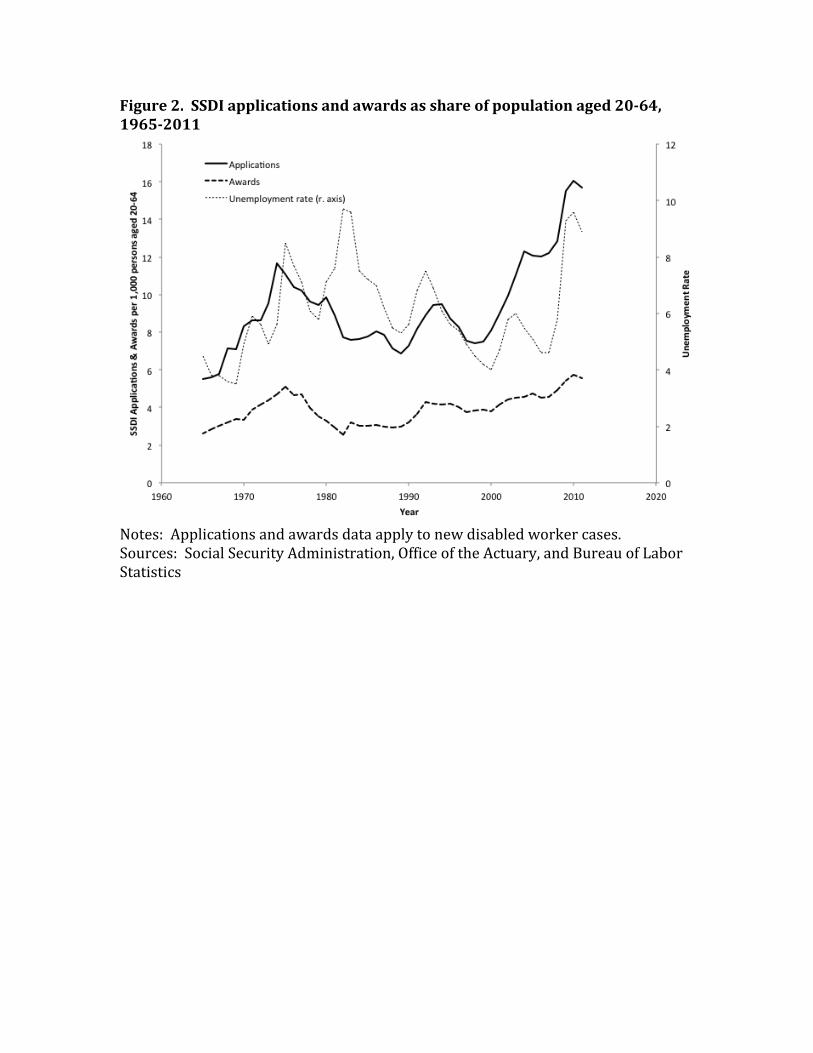
!"#$%&'8)''@@*+'1--6",1/"3.0'1.7'1A1%70'10'021%&'34'-3-$61/"3.'1#&7'89:;<='(>;B:89(('

!"#$%&'!!?--/,+2$,#.&!2.1!242*1&!12$2!2--/<!$#!.%4!1,&23/%1!4#*5%*!+2&%&=!>#0*+%&'!!>#+,2/!>%+0*,$<!?18,.,&$*2$,#.7!@66,+%!#6!$;%!?+$02*<7!2.1!A0*%20!#6!B23#*!>$2$,&$,+&!!

!"#$%&'C)''D3%E&%'-36","&0'FG'7&#%&&'34'7"01F"6"/G'H-I'1.7'J3F:4".7".#'-%3F1F"6"/G'H4I'

'"#$%&'!!>%%!$%C$!6#*!1%&+*,-$,#.!#6!8#1%/=!!@$;%*!8#1%/!-2*28%$%*&!2*%!DE!F!:GH:I!J!H+#**%&-#.1,.K!$#!2!-%*I-%*,#1!42K%!.#*82/,L%1!$#!:!2.1!2!M#3!$;2$!/2&$&!6#*%N%*JO!3P)!F!Q=RO!3()!F!Q=SO!+P!F!Q=TO!+?!F!9O!!!F!Q=USO!2.1!0H<JF<=!!

!"!#

"!$

"!%

"!&

"'()*+

,+-.-/01*213

45-461,17*+

! "# "$ "% "& '()*+,+-.-/01/8,/19:1,;;.-<,=*41->1,;;)*?@5

A@,)<812*)@?@) B;;.01,C@)1@D8,E>=461F:A@,)<8G1/8@41@D-/ B;;.01-HH@5-,/@.0

!"#$%&'<)''@@*+'%&,"-"&./0='@@K'71/1'50)'LM@'K@NL'

!"#$%&'!!>>?!&%*,%&!,.+/01%&!#./<!1,&23/%1!4#*5%*!+2&%&=!!

!"

#$

%&''()*+,-./.,012*34.55.6027

%88& %889 !&&& !&&9 !&%&:,;+

''<*3=6+>,+2*605?7@A'*3;B,*%#C7@A'*3;B,*%#D##E#F7

!"#$%&'B)''O.&P-63GP&./'".0$%1.,&'F&.&4"/'151"61F"6"/G'35&%'/2&'Q%&1/'R&,&00"3.'

!"#$%&'!!V?N%*2K%!&$2$%W!&%*,%&!*%-*%&%.$&!2!&,8-/%7!0.4%,K;$%1!2N%*2K%!2+*#&&!SQ!&$2$%&!-/0&!$;%!(,&$*,+$!2.1!X#/083,2=!!!!

!"#"

$"%"

&""

'(()*+,-+.

/+0(1

(23*+45467407(

"&841!""! "&841!""# "&841!""$ "&841!""% "&841!"&" "&841!"&!943(

:5(;4<(+*343( =616>?>=4@6>?>

!"#$%&';)''N0/"P1/&0'34'/2&'.$PF&%'34'O+'&S21$0/"3.0'-&%'P3./2='899<:89(8)'

!"#$%&'!!V>,80/2$,#.!Y!:&$!%C;20&$,#.W!&%*,%&!,&!+%.&#*%1!2$!:=R!8,//,#.!,.!Z0.%!TQ:QO!$*0%!N2/0%!,&!T=R[!8,//,#.=!!!"#$%&'?)''O+'&S21$0/"3.0'1.7'@@*+'1--6",1/"3.0'FG'P3./2='899<:89(8'

!

!"##

#"##

$###

$"##

$%##

#&'()*'+

,-./

0##1+$ 0##2+$ 0##3+$ 0#$#+$ 0#$0+$4,-./

56-78'(79&':7;+6-';7.7<=6+>87?,-'!'$&.')@/7>&?,-=6+>87?,-'!'A-78')@/7>&?,-

!"!!

#!!

$!!

%%&'()**

+,-).

/01(2"3!!

!1(*45(6

/0783(%9:

!#!!

;!!

<!!

='(4>8)?1./0

1(2"3!!

!1(*45(6

/078:

#!!;6" #!!<6" #!!@6" #!"!6" #!"#6"A/078

='(4>8)?1./012B0)+3(1,6?+)74C:%%&'()**+,-)./01

!"#$%&'T)''O+'&5&./'0/$7"&0'

!!"#$%&'!!\,K0*%!*%-#*$&!+#%66,+,%.$&!#.!1088,%&!6#*!4%%5&!3%6#*%!#*!26$%*!2!P)!%C$%.&,#.!6*#8!*%K*%&&,#.&!$;2$!,.+/01%!&$2$%!2.1!4%%5!6,C%1!%66%+$&!2.1!+03,+!-#/<.#8,2/&!,.!$;%!,.&0*%1!0.%8-/#<8%.$!*2$%!2.1!$;%!$#$2/!0.%8-/#<8%.$!*2$%=!!X#%66,+,%.$&!2*%!*%-#*$%1!,.!?--%.1,C!]23/%&!?=T!2.1!?=9=!

Figure 1: UI Event Studies

(a) Log(SSDI Applications) – All Extensions-.0

4-.0

20

.02

.04

log(

SSDI

App

licat

ions

)

-4 -2 0 2 4Weeks Since UI Ext.

All Ext. Non-Overlapping

(b) Log(SSDI Applications) – 13+ Week Extensions

-.04

-.02

0.0

2.0

4lo

g(SS

DI A

pplic

atio

ns)

-4 -2 0 2 4Weeks Since UI Ext.

All Ext. Non-Overlapping

(c) Acceptance Rate – All Extensions

-.015

-.01

-.005

0.0

05.0

1.0

15Pr

opor

tion

Appr

oved

App

licat

ions

-4 -2 0 2 4Weeks Since UI Ext.

All Ext. Non-Overlapping

(d) Acceptance Rate – 13+ Week Extensions

-.015

-.01

-.005

0.0

05.0

1.0

15Pr

opor

tion

Appr

oved

App

licat

ions

-4 -2 0 2 4Weeks Since UI Ext.

All Ext. Non-Overlapping

!"#$%&'>)''O+'&5&./'0/$7"&0'H(CU'A&&E'.3.:35&%61--".#'&S/&.0"3.0I='FG'1#&'

'"#$%&'!!>%%!.#$%&!$#!\,K0*%!^=!X#%66,+,%.$&!2*%!*%-#*$%1!,.!?--%.1,C!]23/%!?=R=!

Figure 3: UI Event Studies: 13+ Week Extensions – By Age

(a) Log(SSDI Applications)

-.08

-.04

0.0

4.0

8lo

g(SS

DI A

pplic

atio

ns)

-4 -2 0 2 4Weeks Since UI Ext.

20-29 30-4950-64

(b) Acceptance Rate

-.05

-.025

0.0

25.0

5Pr

opor

tion

Appr

oved

App

licat

ions

-4 -2 0 2 4Weeks Since UI Ext.

20-29 30-4950-64

!"#$%&'(&&!)*%&+%,)%+&"-"$.+)+&/0&-"1)/-"$&23&"44$)5"1)/-+

6'7 687 697 6:7 6;7 6<7 6=7 6>7

!"#$%&'(&)*+$,-."/#-&0"#1)*2& 345467 345478 45496 4549: 45498;,%."<%)&/=&>4463?&$@A5B 0454:>B 0454>:B 045448B 045448B 04544CB

D*+$,-."/#-&"#1)*&0$@A5E& 3454>><F)@5&7&;/#.+-B 0454>4B

D*+$,-."/#-&"#1)*&0$@A5E& 45496#)*.&7&;/#.+-B 04549:B

(#"."$%&'(&)*+$,-."/#-&0"#1)*B 34544904544:B

'(&="#$%&<$G-&0"#1)*B 45449045446B

90H/&)*+$,-."/#-&.+"-&;/#.+B 34549C04544?B

'#);<%/G;)#.&F$.)&0IJB 4547C 4547? 45479 4547K 4547K 4547?045447B 045446B 045446B 045446B 045446B 04544KB

%#0"#"."$%&'(&L%$";-B 3454>9 3454>6 3454>6 3454>604549CB 045498B 04549CB 045498B

90M,#)E&M,%GE&J,A,-.&>494B 454>7 454>6 454>> 454>4045448B 045496B 045448B 045448B

N/-.3JOOJ 45498 45479 45498 45498 4549704549?B 045496B 04549?B 04549?B 04549?B

P,$1F$."L&.";)&.F)#1 # G G G G G G GH 949 949 949 949 C6 949 949 949

H/.)-2&&I$;<%)&"#&$%%&L/%,;#-&"-&$&#$."/#$%&.";)&-)F")-&-<$##"#A&J,A,-.&>44:&./&Q)L);R)F&>49>&0H/@);R)F&>44:&./&I)<.);R)F&>49>&"#&L/%,;#&6B5&&Q)<)#1)#.&@$F"$R%)&"-&%#0F)L)"<.-&=/F&II(E&IIQ(E&/F&II(SIIQ(&L%$";-BE&;)$-,F)1&$.&.+)&;/#.+%G&%)@)%&$#1&-)$-/#$%%G&$1T,-.)15&&H)U)G3V)-.&-.$#1$F1&)FF/F-E&$%%/U"#A&=/F&$,./L/FF)%$."/#-&$.&,<&./&=/,F&%$A-E&"#&<$F)#.+)-)-5

!"#$%&'(&&)"*%$&+","&-%.-%//01*/&21-&3345&"66$07",01*/&",&,8%&/,",%9:1*,8&$%;%$

<=> <'> <?> <@> <A> <B> <C> <D> <E>!"#$%&'($#")*+,)#*-./0 12134 12135 12135 12135 12134 12134 12136 12134

-121150 -121150 -121150 -121150 -121150 -121150 -121150 -12115078",&*!9*#:;,<=)8'"=*-8">#:?* @1211A @1211B @1211B @1211C @1211B 12111$<&)8%&#*'D*A11E@4*,FG20 -1211B0 -1211C0 -1211B0 -1211B0 -1211A0 -1211C0

H:;,<=)8'"=*8">#:*-,FG2I* 1211B%+#F2*B*$'");=0 -1211E0

H:;,<=)8'"=*8">#:*-,FG2I* 1211E"#:)*B*$'");=0 -121140

&"-8"8)8,&*!9*J&,8$=0 121B6-121BA0

9"8)8,&*!9*#:;,<=)8'"=*-8">#:0 1211A-1211A0

!9*D8",&*%,(=*-8">#:0 12113-1211A0

3-K'*#:;,<=)8'"=*);8=*$'");0 12131-121140

.),)#*7H ( ( ( ( ( ( ( ( (L'");*7H ( ( ( ( ( ( ( ( (M<N8J*!H*+,)#*J'")+'& (B*&#,>=*,">*&,G=*'D*#:;,<=)8'"*8">#: (H:J&<>#*O<"#@/<G*A131 (K EI3E3 EI3E3 EI3E3 CI6CE CI6CE CIPP6 EI3E3 EI3E3 EI3E3QA 12PP3 12PP3 12PP3 12PP3 12PP3 12PP3 12PP3 12PP3 12PP3

K')#=?**R#%#">#")*F,+8,N&#*8=*&"-+#J#8%)=*'D*..9I*..R9I*'+*..9S..R9*J&,8$=0I*$#,=<+#>*,)*);#*=),)#@N(@$'");*&#F#&*,">*=#,='",&&(*,>T<=)#>2**U,"#&*+,"G#=*D+'$*/<G<=)*A11C*)'*R#J#$N#+*A13A*-K'F#$N#+*A11C*)'*.#%)#$N#+*A13A*8"*J'&<$"=*C*,">*E02**.),">,+>*#++'+=I*J&<=)#+#>*'"*);#*=),)#I*8"*%,+#");#=#=2

!"# !$# !%# !&#!"#$%&'($#")*+,)#*-./0 123224 123225 123224 123224

-232260 -232260 -232260 -23226078",&*!9*#:;,<=)8'"= 2322> 23222

-2322>0 -2322>0?:;,<=)8'"=*8"@#:*-,AB3C*%+#A3*D*$'");=0 23225

-2322D0?:;,<=)8'"=*8"@#:*-,AB3C*"#:)*D*$'");=0 23222

-2322E09"8)8,&*!9*#:;,<=)8'"=*-8"@#:0 12322>

-2322>0!9*F8",&*%,(=*-8"@#:0 23222

-232220.),)#*7? G#= G#= G#= G#=H'");*7? G#= G#= G#= G#=I >5DJ >5DJ >5DJ >5DJKE 2355D 23556 2355D 2355E

I')#=L*M#%#"@#")*A,+8,N&#*8=*);#*,%%+'A,&*+,)#*'F*..M9*,%%&8O,)8'"=*F8&#@C*$#,=<+#@*,)*);#*=),)#1N(1$'");*&#A#&3*P,"#&*+,"B#=*F+'$*Q,"<,+(*E225*1*M#O#$N#+*E2>23*.),"@,+@*#++'+=C*O&<=)#+#@*'"*);#*=),)#C*8"*%,+#");#=#=3

'()*+,%-,.(/+*,0(1(,2+32+4456/4,762,(88269(*,2(1+,(1,1:+,41(1+;<6/1:,*+9+*

!"#$%&'(&&)*++",-&./"/0./01.&23,&+"/14%5&67)89):6&."+;$%<&=>>?8=>@@

9$$ AB%+;$3-%5&"/&#".%&.*,C%-

AB%+;$3-%5&D&AE&%$0F0#$%

:G4"*./&AE&#%23,%&%B5&32&1"$%B5",&-%",

H@I H=I HJI H'I! "#$%&'( &$%&)* '%+'* (%),'

-./01. *&2 #(2 ('2 (,234. #"5* ()5( #&5& #&5'

6&"5$7 6&"5"7 6&&5,7 6&&5,734.8*$9 ("2 "#2 "+2 ")2:;<=0>?@A

BCDE &$2 &'2 &'2 &,2DE (&2 ()2 #&2 #$2E@/.8=@11.4. "+2 ",2 "'2 ",2F39 (&2 &+2 &,2 &'2

B0G@H8I@H=.8J>0><J:/K1@L.; ,*2 $2 $2 $2MA./K1@L.; *2 &$$2 &$$2 &$$2!@>8?A810G@H8I@H=.8N!OB-P "&2 $2 $2 $2

MO8.1?4?G1. (2 ',2 &$$2 &$$2MA./K1@L/.A>8;<H0>?@A%8L.0HJ &5(" &5(& &5#'

N0J8@I8&"Q(&P 6$5*'7 6$5*#7 6$5'(7MO8.RK?H.;8G.I@H.8&"Q(& *,5(2 &$$5$2MO8.RK?H.;8G.I@H.8'Q($ ('5,2 '#5&2C?/.8J?A=.8MO8.RK?H0>?@A%8L.0HJ8 $5,"

N0J8@I8&"Q(&P 6$5*&7EESO8?A=@/.8?A8L.0H8L (5"2 &5#2 &5"2 &5#2EESO8?A=@/.8?A8L.0H8L8?I8A@A.8?A8LT& &5#2 &5$2 $5)2 &5&2

!@>.JU88E>0A;0H;8;.V?0>?@AJ8?A8JW<0H.8GH0=X.>J5883118J>0>?J>?=J8<J.8J0/K1?A48Y.?4Z>J8IH@/8>Z.8?A?>?018/@A>Z1L8[\E8J0/K1.58

!"#$%&'(&&)*"$+,%,&-.&//01&2%3%456&4*&7"638%9&:;/&9"6"

)$$ <*%75( <1&%$4=(>?@ >A@ >B@ >C@ >'@ >D@ >E@ >F@

!"#$#%&"'"#$(&)&#$*!"#$%&'($#")*+,)# -./..0 -./.12 -./.13 -./.14 -./.14 ./2.. -./004 -./025

6./..37 6./.837 6./.0.7 6./.0.7 6./.0.7 6./8297 6./1047 6./1327!:*;<=,+#> -./.98

6./.007!:*?=@#> ./..0

6./..17+$(&,&(-./'/.0#1'2#1"3'*).)-*'4%3.*-13('&$'*51&$67!"#$%&'(#>A!B*#&CD 1/.4 ./.5 -./.8 -./.8

6./127 6./087 6./2.7 6./2.7!"#$%&'(#>A!B*C"#&CD 1/24 1/14 1/14 1/14 1/..

6./147 6./257 6./257 6./257 6./547EBFG*-*>C;,@&#> 2/59 2/59 2/59 2/59

6./.97 6./.97 6./.97 6./.97EBFG*-*"'"->C;,@&#> 8/.4 8/.4 8/.4 8/.4

6./.H7 6./.H7 6./.H7 6./.H7!"#$%/*>=+,)C'"*6(#,+;7A!B*#&CD ./H8 ./H5 ./H5 ./52 ./19

6./137 6./087 6./087 6./2.7 6./257!"#$%/*>=+,)C'"*6(#,+;7A!B*C"#&CD/ ./81 ./81 ./81 ./19

6./8H7 6./8H7 6./8H7 6./0.78+'395&1.)&#$IC$#*;C"?#*!B*#J%C+,)C'"K*(#,+;* -./1H -./1H ./.H ./08

6,;*'L*18M017 6./207 6./207 6./507 6./557!B*#J%C+#>*@#L'+#*9M0. ./85 ./85 ./12 ./89

6./207 6./207 6./297 6./247E 808K443 808K443 808K443 808K443 808K443 808K443 4K81H 2K308NO#+,D#*%+'@,@C&C)(*'L*PB*+#?#C%)*,$'"D*6C"C)C,&&(7*="#$%&'(#>K*C"*%/%/

./4H ./4H ./4H ./4H ./4H ./4H 1/.9 1/8HQLL#?)*'L*6C"*%/%/7R

ST"*="#$%&'($#") ./93 ./93 ./9H ./9H ./54 ./14!B*#J%C+,)C'" ./.1 ./.1 ./.H ./08

E')#;R**I,@&#*+#%'+);*?'#LLC?C#");*6,">*;),">,+>*#++'+;7*L+'$*&'DC)*$'>#&;/**P#%#">#")*O,+C,@&#*C;*,"*C">C?,)'+*L'+*+#?#C%)*'L*UUPB*C"?'$#*>=+C"D*)V#*?,&#">,+*(#,+K*,;*+#%'+)#>*'"*)V#*NUQW/**N&&*;%#?CLC?,)C'";*C"?&=>#*;),)#*X*$'")V*GQ;*,">*>#$'D+,%VC?*?'")+'&;*6,D#K*2*,D#*D+'=%*>=$$C#;K*,">*D#">#+7/**U,$%&#*;%,";*?,&#">,+*(#,+;*8..5-8.11/**B">COC>=,&*&,@'+*L'+?#*;),)=;*C;*>+,T"*L+'$*)V#*@,;#&C"#*$'")V&(*WYU*;,$%&#/**!"#$%&'($#")*>=+,)C'"*,">*#J%C+,)C'"*,+#*$#,;=+#>*,;*'L*P#?#$@#+*01*'L*)V#*(#,+/*W'=")#+L,?)=,&*#LL#?);*C"*@'))'$*+'T;*;#)*!B*#J%C+,)C'"*>,)#*)'*,L)#+*)V#*#">*'L*)V#*(#,+*'+*'T"*&,@'+*L'+?#*;),)=;*)'*#$%&'(#>*6TC)V*="#$%&'($#")*>=+,)C'"*'L*Z#+'7

! "!

!""#$%&'(

#$%!&"'(!)(%"()!*+,!-*+(.!,*&*!*+*./)()!%(./!0+!*!'(*)$%(!01!)"'$.*&(,!23!

(45*$)&"0+)6!!75")!*--(+,"4!,()8%"9()!&5(!)"'$.*&"0+6!

:(!9(;"+!<"&5!,*&*!*&!&5(!)&*&(=<((>!.(?(.!0+!"+"&"*.!8.*"')!10%!23!-*/'(+&)@!

*)!%(-0%&(,!9/!&5(!A'-.0/'(+&!*+,!7%*"+"+;!B,'"+")&%*&"0+!CA7BD6!!:(!,(+0&(!

&5()(!*)!3E)<6!

3+"&"*.!8.*"')!)$9)&*+&"*../!0?(%)&*&(!&5(!+$'9(%!01!*8&$*.!%(8"-"(+&)@!"+!-*%&!

9(8*$)(!)0'(!8.*"'*+&)!*%(!%$.(,!"+(.";"9.(!10%!9(+(1"&)6!#+!*?(%*;(@!*!9"&!.())!&5*+!

5*.1!*)!'*+/!"+"&"*.!-*/'(+&)!*%(!'*,(!*)!&5(%(!*%(!"+"&"*.!8.*"')!1".(,6!!

2+10%&$+*&(./@!A7B!,0()!+0&!-$9.")5!<((>./!)&*&(=.(?(.!,*&*!0+!"+"&"*.!-*/'(+&)6!

75(/!,0!-$9.")5!'0+&5./!,*&*@!50<(?(%6!:(!80'-$&(!&5(!%*&"0!01!"+"&"*.!-*/'(+&)!&0!

"+"&"*.!8.*"')!*&!&5(!)&*&(=9/='0+&5!.(?(.@!*+,!,(+0&(!"&!F)'6!!:(!()&"'*&(!&5(!+$'9(%!

01!"+"&"*.!-*/'(+&)!"+!<((>!<!01!'0+&5!'C<D!*)!3E)<GF)@'C<D6!

H(4&@!<(!8*.8$.*&(!&5(!,*&(!*&!<5"85!*+!"+,"?",$*.!<50!'*>()!*+!"+"&"*.!8.*"'!

"+!)&*&(!)!"+!<((>!<!<"..!(45*$)&!5")!9(+(1"&)@!(C)@<D6!!:(!$)(!0$%!,*&*9*)(!01!23!

%$.()!10%!&5")@!*))$'"+;!&5*&!*..!%(8"-"(+&)!*%(!(.";"9.(!10%!&5(!1$..!,$%*&"0+!01!9(+(1"&)!

*+,!&5*&!&5(/!,%*<!9(+(1"&)!80+&"+$0$)./!1%0'!<!$+&".!(45*$)&"0+6!!!

B)!+0&(,!"+!&5(!&(4&@!<(!80+)",(%!&<0!,(1"+"&"0+)!01!(45*$)&"0+I!75(!1"%)&!

<((>!"+!<5"85!9(+(1"&)!*%(!+0&!%(8("?(,!*&!&5(!$)$*.!&"'(@!*+,!&5(!1"%)&!<((>!"+!

<5"85!&5(/!*%(!+0&!%(8("?(,!("&5(%!"+"&"*../!0%!%(&%0*8&"?(./6!75(!,")&"+8&"0+!*%")()!

1%0'!&5(!&('-0%*%/!(4-"%*&"0+)!01!&5(!A2E!-%0;%*'!"+!JKLKI!M*+/!%(8"-"(+&)!*%(!

80$+&(,!*)!(45*$)&"+;!,$%"+;!&5()(!(4-"%*&"0+)!9/!&5(!1"%)&!,(1"+"&"0+!9$&!*1&(%<*%,!!

9/!&5(!)(80+,6!M0)&!01!0$%!*+*./)")!$)()!&5(!)(80+,!,(1"+"&"0+6!

! ""!

75(%(!*%(!8*)()!<5(%(!%(8"-"(+&)!(45*$)&!&5("%!9(+(1"&)@!(4-(%"(+8(!-(%"0,)!

01!+0+=-*/'(+&)@!&5(+!9(80'(!(.";"9.(!10%!*,,"&"0+*.!9(+(1"&)!.*&(%6!75")!8*+!5*--(+!

<5(+!+(<!A2E!&"(%)!*%(!*,,(,!10%!<5"85!-*)&!(45*$)&(()!*%(!(.";"9.(6!3&!8*+!*.)0!

*%")(!10%!AN!%(8"-"(+&)!,$%"+;!*+,!*1&(%!&5(!JKLK!&('-0%*%/!A2E!(4-"%*&"0+)I!!M*+/!

)&*&()!(+,(,!AN!-*/'(+&)!,$%"+;!&5()(!(4-"%*&"0+)@!&5(+!%(O0"+(,!<5(+!&5(!

-%0;%*'!<*)!%(*$&50%"P(,!C*+,!&5(!LKKQ!1(,(%*.!AN!)5*%(!)"'$.&*+(0$)./!

%("+)&*&(,D6!R(8"-"(+&)!<50)(!AN!-*/'(+&)!<(%(!"+&(%%$-&(,!<(%(!+0&!%(-*",!

%(&%0*8&"?(./6!N0&5!01!0$%!,(1"+"&"0+)!80$+&!&5()(!%(8"-"(+&)!*)!5*?"+;!(45*$)&(,!

&5("%!9(+(1"&)!0+!&5(!1"%)&!<((>!10%!<5"85!9(+(1"&)!<(%(!+0&!-*",6!

#1!80$%)(@!'0)&!8.*"'*+&)!,0!+0&!%('*"+!"+!$+('-.0/'(+&!$+&".!(45*$)&"0+@!

("&5(%!9(8*$)(!&5(/!;(&!O09)!9(10%(5*+,!0%!9(8*$)(!&5(/!(4"&!&5(!.*90%!10%8(6!!:(!

()&"'*&(!&5(!-%09*9"."&/!&5*&!*+!"+,"?",$*.!<50!,%(<!5")!"+"&"*.!-*/'(+&!"+!<((>!<!

)$%?"?()!&0!(45*$)&!5")!9(+(1"&)!,!S!(C)@<D=<!<((>)!.*&(%!*)!

CBLD! TC,U!)@<D!S! !! ! !!!!! ! !!!!!!! @!

<5(%(!! !!!! ! !%(-%()(+&)!&5(!-%09*9"."&/!&5*&!*+!"+,"?",$*.!"+!)&*&(!)!<"&5!

$+('-.0/'(+&!,$%*&"0+!,!"+!<((>!?!(4"&)!$+('-.0/'(+&!C9/!1"+,"+;!*!+(<!O09!0%!

9/!(4"&"+;!&5(!.*90%!10%8(D!9/!<((>!?VL6!

70!()&"'*&(!&5(!5*P*%,!1$+8&"0+@!<(!9(;"+!<"&5!'0+&5./!,*&*!0+!"+"&"*.!*+,!

1"+*.!-*/'(+&)!"+!&5(!%(;$.*%!23!-%0;%*'@!<5"85!011(%)!JW!<((>)!01!9(+(1"&)6!!X(&!-'!

%(-%()(+&!&5(!%*&"0!01!1"+*.!-*/'(+&)!"+!'0+&5!'VY!&0!"+"&"*.!-*/'(+&)!"+!'0+&5!'@!

80'-$&(,!10%!&5(!+*&"0+!*)!*!<50.(6!!75")!8*+!9(!)((+!*)!*+!()&"'*&(!01!&5(!JW=<((>!

)$%?"?*.!-%09*9"."&/6!!:(!)'00&5!"&!9/!()&"'*&"+;!*!&"'(!)(%"()!%(;%())"0+!01!-'!0+!*!

Y&5!0%,(%!-0./+0'"*.!"+!8*.(+,*%!&"'(@!<"&5!'0+&5=01=/(*%!C)(*)0+*."&/D!(11(8&)!

! """!

%('0?(,6!X(&!&5(!1"&&(,!?*.$(!C+(&!01!&5(!)(*)0+*."&/!(11(8&)D!9(!!!6!#$%!"+"&"*.!

()&"'*&(!01!&5(!5*P*%,!")!9*)(,!0+!&5(!JW&5!%00&!01!&5")I!

CBJD!! !! !!!! ! ! !! !! ! !!! !"6!

Z(%(@!'C?D!")!&5(!'0+&5!80+&*"+"+;!<((>!?U!<(!)5"1&!&5")!9/![!&0!8*-&$%(!&5(!'0+&5!

"+!&5(!'",-0"+&!01!&5(!-(%"0,!80?(%(,!9/!&5(!)"4='0+&5!)$%?"?*.!,*&*6!

H0&(!&5*&!&5")!"+"&"*.!5*P*%,!()&"'*&(!,0()!+0&!?*%/!<"&5!,$%*&"0+!01!

$+('-.0/'(+&@!<5(%(!&5(!(?",(+8(!"+,"8*&()!&5*&!$+('-.0/'(+&!(4"&!5*P*%,)!*%(!

5";5(%!10%!&5(!)50%&=&(%'!$+('-.0/(,!&5*+!10%!&5(!.0+;=&(%'!$+('-.0/(,6!:(!,%*<!

()&"'*&()!01!&5(!,$%*&"0+!-%01".(!1%0'!R0&5)&("+\)!CJKLLD!*+*./)")!01!(4"&!5*P*%,)!"+!

E]T!,*&*@!*)!)$''*%"P(,!9/!5")!F";$%(!Y6!:(!$)(!&5(!E]T!,*&*!&0!80'-$&(!(4"&!

5*P*%,)!10%!&5%((!,$%*&"0+!;%0$-)!C,^L[@!L[_,^JW@!*+,!,`JWD!%(.*&"?(!&0!&5(!

*?(%*;(!(4"&!5*P*%,!0?(%!&5(!1"%)&!JW!<((>)@!&%(*&"+;!&5(!-(%"0,)!9(10%(!*+,!*1&(%!

a*+$*%/!L@!JKKb!)(-*%*&(./6!N/!80'-*%"+;!&5(!(4"&!5*P*%,!"+!(*85!,$%*&"0+!;%0$-!&0!

&5(!*?(%*;(!(4"&!5*P*%,!10%!&50)(!<"&5!,^JW@!<(!09&*"+!'$.&"-."8*&"?(!1*8&0%)!10%!$)(!

"+!*,O$)&"+;!!cK6!!75()(!.(*,!$)!&0!0$%!*,O$)&(,!5*P*%,)I!

CB[D!! ! !!!! ! !

!!!"# ! !!!!!!! !! !"#! ! !"!!"#!! ! !!!!!""#!!!"# ! !!!!!!! !! !"#! ! !"!!"#!! ! !!!!!""#!!!"# ! !!!!!!! !! !"#!" ! ! ! !"!!"#!! ! !!!!!""#!!!"# ! !!!!!!! !! !"#!" ! ! ! !"!!"#!! ! !!!!!""#!!!"# ! !!!!!!! !! !"#!" ! !!!"#!! ! !!!!!""#!!!"# ! !!!!!!! !! !"#!" ! !!!"#!! ! !!!!!""#!

!

#$%!1"+*.!)"'$.*&(,!23!(45*$)&"0+!'(*)$%(!10%!)&*&(!)@!<((>!&!")!80'9"+()!

"+"&"*.!8.*"')@!-*/'(+&!%*&()@!*+,!)$%?"?*.!&0!(45*$)&"0+6!F0%'*../@!"&!")I!

CBdD! !!" ! !"!" ! !!!! ! ! !! ! !! !!! ! !! !!! !!!!!!! !! !!! !! !

!

!"# !$# !%# !&# !'# !(# !)# !*# !+# !",# !""# !"$#!"#$%&'($#")*+,)#*-./0 12134 12135 12134 12134 12116 12114 12133 12131 12114 12115 12114 12114

-121150 -121150 -121150 -121150 -121150 -121150 -121150 -121150 -121170 -121170 -121170 -12117089",&*!:*#;<,=>)9'"> ?1211@ ?12117 ?12133 ?12131 12111 12111

-1211A0 -1211A0 -1211B0 -121170 -1211@0 -121130C;<,=>)9'">*9"D#;*-,EF2G 1211A ?12131 ?12115***%+#E2*A*$'")<>0 -1211B0 -121310 -121170C;<,=>)9'">*9"D#;*-,EF2*G 1211B 12111 1211A**"#;)*A*$'")<>0 -121140 -121140 -121170:"9)9,&*!:*#;<,=>)9'">*-9"D#;0 1211@ 12111 12113

-1211@0 -121130 -121130!:*H9",&*%,(>*-9"D#;0 12113 12111 ?12113

-1211@0 -121130 -121130.),)#*8C I#> I#> I#> I#> I#> I#> I#> I#> I#> I#> I#> I#>J'")<*8C I#> I#> I#> I#> I#> I#> I#> I#> I#> I#> I#> I#>K B3B3 7L7B B3B3 B3B3 3LA5 3LA5 3LA5 3LA5 3LA5 3LA5 3LA5 3LA5M@ 12663 12663 12663 12663 12667 12667 12667 12667 12664 12664 12664 12664

K')#>N*O#%#"D#")*E,+9,P&#*9"*Q'&=$">*3?L*9>*&"-+#R#9%)>*H'+*..:G*..O:G*'+*..:S..O:*R&,9$>0*H+'$*%=P&9R&(*,E,9&,P&#*),P=&,)9'">*P(*>),)#*,"D*$'")<T*D#%#"D#")*E,+9,P&#*9"*Q'&=$">*6?3@*9>*&"-,%%&9R,)9'">*H'+*..O:0*R'$%9&#D*H+'$*,D$9"9>)+,)9E#*$9R+'*D,),*H9&#>2*U,"#&*+,"F#>*H+'$*/=F=>)*@117*?*O#R#$P#+*@13@*H'+*Q'&=$">*3?7*,"D*H+'$*V,"=,+(*@11L*?*O#R#$P#+*@131*H'+*)<#*+#$,9"9"F*R'&=$">2*.),"D,+D*#++'+>G*R&=>)#+#D*'"*)<#*>),)#G*9"*%,+#")<#>#>2

-./01234"25.61027.8.291:91;;<=6;2>=92??@A2.BB0<C.8<=6;2.828D12;8.81EF=68D201G10H2C=FB.9<6:291;I08;2J<8D27<>>1916827.8.2;=I9C1;2.6728<F12B19<=7;

5I/0<;D1727.8.KI002;.FB01 $,,*E$,",

5I/0<;D1727.8. 37F<6<;89.8<G12><01;$,,*E$,",

!"#$ %&'()*$ !"#$ %&'()*$ !"#$ %&'()*$ !"#$ %&'()*$!""#$%&$'()"*+,%* -./..0 $1./.234$ -./.50 $1./67.4$ -./.50 $1./.634$ -./.89 $1./5554$

:./.5.; $ :./.53; $ :./.53; $ :./.57; $5$!""#$<%+)$'()"*+,%* ./..0 $1./6524$ ./..0 $1./7=.4$ ./.59 $1./2964$ ./..9 $1./6224$

:./.5.; $ :./..2; $ :./.56; $ :./.5.; $8$!""#+$<%+)$'()"*+,%* -./.57 $1./.534$ ./..8 $1./2554$ -./.56 $1./.364$ ./..9 $1./7934$

:./.58; $ :./.59; $ :./.57; $ :./.8.; $6$!""#+$<%+)$'()"*+,%* -./.52 $1./..84$ -./..2 $1./0634$ -./.58 $1./.664$ -./..5 $1./2.24$

:./.5.; $ :./.58; $ :./.53; $ :./.50; $0$!""#+$<%+)$'()"*+,%* -./.53 $1./.384$ -./..5 $1./2624$ -./.55 $1./5864$ -./.59 $1./6904$

:./.58; $ :./.58; $ :./.59; $ :./.59; $5$!""#$<>"$'()"*+,%* ./..2 $ -./..3 $ ./..3 $ -./.5. $

:./.56; $ :./.58; $ :./.50; $ :./.58; $8$!""#+$<>"$'()"*+,%* ./.52 $ -./..9 $ ./.6= $ ./..0 $

:./.58; $ :./.50; $ :./.58; $ :./.5.; $6$!""#+$<>"$'()"*+,%* ./.65 $ ./.5. $ ./.86 $ ./..3 $

:./.50; $ :./.59; $ :./.57; $ :./.57; $0$!""#+$<>"$'()"*+,%* ./..5 $ ./..5 $ ./..0 $ -./..9 $

:./.5.; $ :./.57; $ :./.55; $ :./.57; $?,&&">"*@"$,*$AB">CD"$:.$)%$0$B+$-5$)%$-0; -./.83 -./..0 -./.80 -./..0<-ECFG" 1./.874 1./2554 1./.704 1./02=4AB">CD"$:.$)%$0$H""#+; -./.5. -./..0 -./..9 -./..7<-ECFG" 1./0504 1./254 1./8554 1./07=4I%*-JB">FCKK,*D$'()"*+,%*+$J*FL I% M"+ I% M"+56N$!""#$'()"*+,%*+$J*FL I% I% M"+ M"+O)C)"$P' ( ( ( (Q,R"$P' ( ( ( (SGT,@$,*$U*+G>"V$W*"RK/$XC)" ( ( ( (SGT,@$,*$W*"RKF%LR"*)$XC)"$:OA; ( ( ( (I =..9 =..9 =..9 =..9X8 ./2=2 ./2=2 ./2=2 ./2=2

+(!)$,-./,0'$12,#2*34,5$65$##781#,985,)1:1*;!$5,89,<<=>,(%%)7?(2781#@

I%)"+Y$?"K"*V"*)$BC>,CTF"$,+$F*:OO?U$CKKF,@C),%*+;Z$R"C+G>"V$C)$)["$+)C)"-TL-H""#$F"B"F/$<C*"F$>C*D"+$&>%R$\C*GC>L$8..=$-$?"@"RT">$8.5./$O)C*VC>V$">>%>+Z$@FG+)">"V$%*$)["$+)C)"Z$,*$KC>"*)["+"+/$<-BCFG"+$%&$)"+)+$%&$K%+)-"()"*+,%*$VGRR,"+$CDC,*+)$)["$CB">CD"$%&$K>"-"()"*+,%*$VGRR,"+$C>"$,*$+]GC>"V$T>C@#")+/

:A@:B@:/@:C@

!"#$ %&'()*$ !"#$ %&'()*$ !"#$ %&'()*$ !"#$ %&'()*$!""#$%&$'()"*+,%* -./..0 $1./23.4$ -./..5 $1./3634$ ./..0 $1./7874$ ./..7 $1./3274$

9./..7: $ 9./..6: $ 9./..5: $ 9./.;.: $;$!""#$<%+)$'()"*+,%* ./..; $1./0=64$ ./... $1./=.74$ -./..7 $1./==24$ -./..8 $1./58.4$

9./..=: $ 9./..5: $ 9./..=: $ 9./..=: $8$!""#+$<%+)$'()"*+,%* ./..= $1./;534$ ./.;7 $1./.804$ ./..= $1./87.4$ ./.;0 $1./;;34$

9./..6: $ 9./..3: $ 9./..3: $ 9./..=: $0$!""#+$<%+)$'()"*+,%* -./..8 $1./66;4$ -./..3 $1./=0.4$ ./..7 $1./05.4$ ./..0 $1./6224$

9./..=: $ 9./..2: $ 9./..=: $ 9./..6: $7$!""#+$<%+)$'()"*+,%* -./..7 $1./6574$ ./... $1./5;24$ -./..8 $1./2264$ ./..; $1./2604$

9./..=: $ 9./..5: $ 9./..=: $ 9./..6: $;$!""#$<>"$'()"*+,%* -./.;0 $ -./..6 $ -./.;0 $ -./..5 $

9./..5: $ 9./..5: $ 9./..=: $ 9./..=: $8$!""#+$<>"$'()"*+,%* ./..= $ ./..6 $ ./..8 $ ./.;. $

9./..5: $ 9./..=: $ 9./..=: $ 9./..6: $0$!""#+$<>"$'()"*+,%* -./..= $ -./..3 $ ./..0 $ ./..7 $

9./..7: $ 9./..7: $ 9./..5: $ 9./..=: $7$!""#+$<>"$'()"*+,%* ./..8 $ -./..= $ ./..; $ -./..0 $

9./..3: $ 9./..5: $ 9./..=: $ 9./..5: $?,&&">"*@"$,*$AB">CD"$9.$)%$7$B+$-;$)%$-7: ./..0 ./..0 ./..0 ./..8<-ECFG" 1./3.=4 1./8;64 1./8604 1./734AB">CD"$9.$)%$7$H""#+: ./... ./... ./..; ./..7<-ECFG" 1./=0=4 1./0584 1./0264 1./8624I%*-JB">FCKK,*D$'()"*+,%*+$J*FL I% M"+ I% M"+;0N$!""#$'()"*+,%*+$J*FL I% I% M"+ M"+O)C)"$P' ( ( ( (Q,R"$P' ( ( ( (SGT,@$,*$U*+G>"V$W*"RK/$XC)" ( ( ( (SGT,@$,*$W*"RKF%LR"*)$XC)"$9OA: ( ( ( (I 6..3 6..3 6..3 6..3X8 ./38 ./30 ./38 ./30

I%)"+Y$?"K"*V"*)$BC>,CTF"$,+$)Z"$C@@"K)C*@"$>C)"[$R"C+G>"V$C)$)Z"$+)C)"-TL-H""#$F"B"F/$<C*"F$>C*D"+$&>%R$\C*GC>L$8..6$-$?"@"RT">$8.;./$O)C*VC>V$">>%>+[$@FG+)">"V$%*$)Z"$+)C)"[$,*$KC>"*)Z"+"+/$<-BCFG"+$%&$)"+)+$%&$K%+)-"()"*+,%*$VGRR,"+$CDC,*+)$)Z"$CB">CD"$%&$K>"-"()"*+,%*$VGRR,"+$C>"$,*$+]GC>"V$T>C@#")+/

+(!)$,-./,0'$12,#2*34,5$65$##781#,985,(::$%2(1:$,5(2$

;<= ;>= ;/= ;?=

!"# !$# !%# !&# !'# !(#!""#$%&$'()"*+,%* -./.01 ./.12 -./.34 ./..4 -./.35 -./..3

6./.227 6./.057 6./.087 6./.427 6./.037 6./.4474$!""#$9%+)$'()"*+,%* ./.01 -./..5 ./.0: ./..1 -./..4 -./..2

6./.507 6./.317 6./.087 6./.437 6./.417 6./..:70$!""#+$9%+)$'()"*+,%* -./.38 -./.08 ./.00 -./.01 ./..5 ./.05

6./.537 6./.1.7 6./.317 6./.457 6./.047 6./..;73$!""#+$9%+)$'()"*+,%* -./.02 -./.12 ./.4. ./... ./..0 ./..4

6./.257 6./.0:7 6./.027 6./.437 6./.457 6./.4.71$!""#+$9%+)$'()"*+,%* -./.8; -./.03 ./.32 -./..0 -./.0; ./..:

6./.237 6./.0;7 6./.087 6./.487 6./.057 6./..874$!""#$9<"$'()"*+,%* -./.41 -./.02 ./..8 ./..: -./.01 -./..8

6./.1:7 6./.017 6./.007 6./.437 6./.487 6./..870$!""#+$9<"$'()"*+,%* ./.0. ./.0: ./.32 ./.3: -./.43 ./..5

6./.187 6./.057 6./.047 6./.407 6./.427 6./.4.73$!""#+$9<"$'()"*+,%* -./.1. -./.00 -./.3: -./..0 ./.08 ./..2

6./.247 6./.307 6./.357 6./.007 6./.457 6./..571$!""#+$9<"$'()"*+,%* -./.00 -./.3: -./..1 -./.04 -./..3 -./..2

6./.2:7 6./.0;7 6./.307 6./.417 6./.4:7 6./..57=,&&"<"*>"$,*$?@"<AB"$6.$)%$1$@+$-4$)%$-17 -./.41 ./..3 ./.43 -./.4 -./..: ./..59-CADE"$%&$F%,*)$G,B*,&,>A*>"$)"+) H$./:50$I H$./012$I H$./1;.$I H$./2:3$I H$./838$I H$./.38$I=,&&"<"*>"$,*$?@"<AB"$6.$)%$1$@+$.7 -./.0: -./.44 ./.43 -./..1 -./.40 ./..29-CADE"$%&$F%,*)$G,B*,&,>A*>"$)"+) H$./818$I H$./13.$I H$./153$I H$./2;.$I H$./580$I H$./.45$IJ%*-K@"<DALL,*B$'()"*+,%*+$K*DM N"+ N"+ N"+ N"+ N"+ N"+43O$!""#$'()"*+,%*+$K*DM N"+ N"+ N"+ N"+ N"+ N"+G)A)"$P' ( ( ( ( ( (Q,R"$P' ( ( ( ( ( (SET,>$,*$U*+E<"V$W*"RL/$XA)" ( ( ( ( ( (SET,>$,*$W*"RLD%MR"*)$XA)"$6G?7 ( ( ( ( ( (J 850. 850. :..3 :..3 :..8 :..8X0 ./:5 ./4: ./;8 ./21 ./;: ./23

)*+,-./0&.12-34.54678.9-:9-55;<35.=<9.,3!36>+-9.<=.??@A.*BB,;C*4;<35#.*37.*CC-B4*3C-.9*4-.+8.*:-.:9<6B

/:-.$DE$F /:-.%DE&F

J%)"+Y$="L"*V"*)$@A<,ATD"$,+$D*6*ERT"<$%&$GG=U$ALLD,>A),%*+7$&%<$>%DER*+$4Z$3$A*V$2$A*V$)["$A>>"L)A*>"$<A)"$&%<$>%DER*+$0Z$1$A*V$5/$9A*"D$<A*B"+$&<%R$FA*EA<M$0..:$-$=">"RT"<$0.4./$G)A*VA<V$"<<%<+Z$>DE+)"<"V$%*$)["$+)A)"Z$,*$LA<"*)["+"+/$9-@ADE"+$%&$)"+)+$%&$L%+)-"()"*+,%*$VERR,"+$ABA,*+)$)["$A@"<AB"$%&$L<"-"()"*+,%*$VERR,"+$A<"$,*$+\EA<"V$T<A>#")+/

/:-.'DE('