unequal opportunities and human capital formation€¦ · · 2009-09-22unequal opportunities and...

Unequal opportunities and humancapital formation

Daniel Mejía Marc St-Pierre

January, 2004

Preliminary draft

Abstract

This paper develops a tractable, heterogeneous agents general equi-librium model where agents face different costs of access to the edu-cational system. The paper explores the relation between inequality ofopportunities (in the form of differential costs of access to the educa-tional process) and efficiency (the levels of human capital and output) .In particular, the results from the simulations of the model suggest thata higher level of inequality of opportunities is associated with a lowerlevel of average human capital, lower output per worker and higher in-come (wage) inequality. In other words, the model (based on standardassumptions) does not predict a trade-off between efficiency and equalopportunity in human capital formation.

0D. Mejía: Brown University and Banco de la República, Colombia, M. St-Pierre: BrownUniversity. We are grateful to Pedro Dal Bó, Oded Galor, Peter Howitt, Tom Krebs, HeraklesPolemarchakis and participants at the Macro Lunch at Brown University for many helpfulsuggestions.

1. Introduction

Most of the literature that studies the effects of income inequality on economicgrowth through its effects on human capital has focused on the role of creditconstraints. The main idea of this line of research is the following: relatively pooragents don’t have the means to finance the accumulation of human capital and,because they are credit constrained (that is, there is no way to finance the costsof human capital accumulation using future earnings as the collateral for a loan topay the tuition fees), they end up either not investing in human capital or investingvery little. Furthermore, if there are decreasing returns to the accumulation ofhuman capital the final outcome does not maximize the size of the economicpie and therefore there may be scope for redistribution of resources from rich topoor individuals which, in turn, increases the size of the pie. This redistributionreallocate resources towards more profitable investments given that the returns tohuman capital accumulation are higher for those individuals (the relatively poorones) who have less human capital. The theoretical idea has been extensivelydeveloped in the literature since the work by Galor and Zeira (1993) and Banerjeeand Newman (1993). Further developments have been proposed by De Gregorio(1995) and Bénabou (1996, 2000). Empirical evidence has been found in favor ofthe hypothesis that inequality and credit constraints affect human capital by Fluget al. (1998), De Gregorio (1995) and Mejía (2003).

But the accumulation of human capital involves other complementary factorsas well. This has been extensively documented in a number of recent empiricalstudies, some of which will be resumed in the next section. While some of thesefactors can be thought as being non-purchasable (neighborhood effects shapedby local communities, family background, socioeconomic characteristics, genes, provision of social connections, installation of preferences and aspirations inchildren), others are not (pre and post natal care, parent’s level of education,distance to schools and different qualities of books, teachers and schools) 1.If the previously mentioned factors are important in determining differences in

educational attainment across individuals, the distribution of this “socio-economiccharacteristics” across individuals matters. In other words, if the distribution ofaccess to the schooling system is important, one should encounter differences ineducational attainment across individuals, even in economies with complete cover-age of public school provision. This does not rule out the importance of the lack of

1See Roemer (2000), Bénabou (2000) and Dardanoni et al. (2003), among others.

2

financial resources to pay for the (monetary) costs of education2. As said before,different studies have already shown that they are in fact important. However,this paper emphasizes the effects of inequality of access to the schooling system onhuman capital accumulation decisions made by individuals. Also, the model ad-dresses the equilibrium relation between inequality of opportunity and efficiency.More precisely, the model is used to study the relation between inequality of op-portunities and efficiency, the latter measured by output per capita or per capitahuman capital.

The paper is organized as follows: the second section reviews the empiricalevidence regarding the effects of some of the complementary factors mentionedabove on educational outcomes. The third section presents the model and thefourth section the results of the simulation of the model using a (well behaved)distribution function to simulate different degrees of inequality of opportunity.The last section presents the main conclusions derived from the paper.

2. Empirical evidence on the determinants of human capital

Since the publication of the Coleman Report (Coleman et al., 1966) hundreds ofpapers have studied the relationship between school expenditure and the effectsof complementary factors on different measures of educational outcomes in theUnited States. More precisely, The Coleman Report found that the socioeco-nomic composition of the student body had a significant effect on test scores aftercontrolling for student background, school and teacher characteristics (Ginther etal., 2000). This findings attracted the attention of scholars and policymakers asone of its main conclusions was that schools characteristics were relatively unim-portant in determining achievement, while family characteristics were found tobe the main determinant of student success or failure (Hanushek, 1996). Sincethen, many studies have used different data sets and econometric specificationsto improve the estimates of the effects of family background, parental education,neighborhood effects and many other socioeconomic characteristics on educational

2Family income has been found to have large explanatory power on longitudinal studiesof educational outcomes accross individuals. However, family income or assets do not onlyaffect the individual’s capacity to pay for tuition costs but also many other factors such as theneighborhood where the kids grow up, their health, and the capacity to buy complementaryfactors to the educational process.

3

outcomes3. In a study with more than 5,000 undergraduates at UC San DiegoBetts and Morell (1997) found that personal background (family income and race)and the demographic characteristics of former high school classmates, significantlyaffected the student’s GPA. This result was obtained after controlling for the de-gree program in which the students were enrolled and the resources of the highschool attended. Moreover, they found that school effects partially reflected theincidence of poverty and the level of education among adults in the school neigh-borhood. In a different paper Golghaber and Brewer (1997) found that familybackground characteristics had a significant effect on tests scores taken by 18,000students in the 10th grade, even after controlling for school characteristics andthe results on a previously taken math test by the same students. They found,for instance, that years of parental education and family income were positivelyrelated to test scores. Also, Blacks, Hispanic and kids coming from a family withno mother in the household had, on average, a lower predicted score in the mathtest. Another study by Groger (1997) found empirical evidence on the negative(and significant) effects of local violence on the likelihood of graduating from highschool. While the average dropout rate in his sample is 21 percent, minor vio-lence increases the dropout rate by 5 percentage points, moderate levels of violenceraises it by 24 percent and substantial violence by 27 percent.

Data requirements in longitudinal studies to estimate the effects of schoolcharacteristics, family background and neighborhood effects on educational out-comes constitutes the main constraint to undertake research on the determinantsof educational outcomes in developing countries. However, the use of random-ized experiments to estimate the effects of changes in the complementary factors(such as: improving health conditions, provide educational inputs, and lower thecosts associated with school attendance, among others) on different measures ofeducational outcomes has become one of the hottest topics in the developmentliterature4. The list of recent papers that evaluate the effects of improving theaccessibility of these complementary factors is growing rapidly and a completesurvey of their findings is not the purpose of this article. However, some examplesare worth mentioning.

3For a reviw of the literature, as well as the main findings (and econometric specificationproblems) the reader is refered to Ginther et al. (2000) and Hanushek (1986 and 1996). Thepaper by Durlauf (2002) presents a complete review of how social interactions play an importantrole on the perpetuation of poverty, altough, not only through the human capital channel.

4The reader is refered to Duflo and Kremer (2003) and Kremer (2003) for a review of themethodology of randomized experiments as well as their main findings.

4

One of this randomized experiments evaluates the effects of mass dewormingin 75 school populations in Kenya. The results are very clear: “Health and schoolparticipation improved not only at program schools, but also at nearby schools,due to reduced disease transmission. Absenteeism in treatment schools was 25%(or 7 percentage points) lower than in comparison schools. Including this spillovereffect, the program increased schooling by 0.15 years per person treated.” (KremerandMiguel, 2001). The same pattern of results were found in a similar randomizedexperiments in India (Bobonis et al., 2002, cited in Kremer, 2003).In another randomized experiment conducted in Colombia, vouchers to cover

more than half of the tuition costs of secondary education in private schools weredistributed by lottery to kids in secondary school age from neighborhoods classifiedas falling in to the two lowest socioeconomic strata5. The effects of the programwere estimated by Angrist et al. (2003) by measuring the differences in certaincharacteristics and test scores between voucher winners and a control group ofnonparticipants in the program. After three years in the program, voucher winnerswere 15 percentage point more likely to have attended a private school, were 10%more likely to have completed the 8th grade and scored 0.2 standard deviationshigher on standardized tests given to the whole population (voucher winners pluscontrol group of nonparticipants in the program)6.From the empirical evidence presented above it is clear that the role played

by complementary factors in the educational process is in fact important. In thefollowing section we construct a model where the degree of inequality of access tothe schooling system is a first order determinant of the levels of human capitaland other economic variables.

3. The basic structure of the model

Consider a small economy operating under perfectly competitive markets. Theproduction of the (single) final good is determined by a neoclassical productionfunction that combines physical capital, human capital and unskilled labor.

5Neighborhoods in Colombia are stratified from 1 (the poorest) to 6 (the richest), mainly forpurposes of setting utilities tariffs in a progressive manner.

6Other randomized experiments include: PROGRESA in Mexico (Schultz, forthcoming),School meals in Kenya (Kremer and Vermeersch, 2002), Provision of uniforms, textbooks andclassroom construction in Kenya (Kremer et al., 2002), Provision of a second teacher (if possible,female) in one-teacher schools in India (Banerjee and Kremer, 2002).

5

Individuals are identical regarding their preferences and abilities but may dif-fer with regard to the cost they face of acquiring human capital because they havedifferent access to the complementary factors of the educational process, just asexplained in the previous section. In that sense, individuals face unequal opportu-nities of acquiring human capital. The distribution of this costs across individualsis assumed to be exogenously given. Given the costs of acquiring human capital,each individual decides how much time to devote to acquire human capital (ifany), and then compares the income she would receive if she decides to work as askilled worker with that one she would receive if she decides not to acquire humancapital and work as an unskilled worker. In equilibrium, the aggregate level ofhuman capital as well as the output level are determined by the distribution ofthe costs of acquiring human capital as well as on other parameters of the model.Although unequal access to the complementary factors of the educational

process can be partially linked to wealth or income inequality, there are somepredetermined characteristics of individuals that cannot be modified and/or can-not be purchased in the market once the time to make investment decisions ineducation comes: pre and post-natal care, neighborhood effects, parental level ofeducation, school quality, among others. In order to concentrate on the effectsof inequality of opportunities on human capital investment decisions, it will beassumed that all individuals are endowed with the same share of the total capitalstock of the economy and education is provided free.

3.1. Production technology and firm’s optimization conditions

The technology of production of final goods combines unskilled labor, skilled labor(human capital) and physical capital according to a neoclassical production func-tion characterized by aggregate constant returns to scale and diminishing marginalreturns on each one of the factors of production (equation 3.1)

Y = F (Lu, H,K) = (Lu)α (H)βK1−α−β (3.1)

Where Lu is the proportion of individuals who work as unskilled labor, H istotal human capital in the economy, determined by H = Ls

_

hs, where Ls is theproportion of individuals that acquire human capital and,

_

hs is the average levelof human capital across those individuals that accumulate human capital andtherefore work as skilled workers. K is the aggregate capital stock. For the sakeof simplicity it is assumed that the total population consists of a continuum ofindividuals of size 1. Therefore Lu + Ls = 1.

6

Markets are perfectly competitive and firms choose the number of unskilledand skilled workers they hire as well as physical capital in order to maximizeprofits. The inverse demand for each one of the factors of production is given inequations 3.2 to 3.4.

wu = α(Lu)α−1(H)βK1−α−β (3.2)

ws = β (Lu)α (H)β−1K1−α−β (3.3)

r = (1− α− β) (Lu)α (H)βK−α−β (3.4)

Where wu is the unskilled wage rate, ws is the wage rate per unit of humancapital (defined later on) and r is the interest rate.

3.2. Individual’s human capital decision and occupational choice

Individuals are identical in their preferences and abilities and each of them is en-dowed with one unit of time which they allocate between working and acquiringhuman capital (if any). However, individuals may differ in the costs they face perunit of human capital accumulated. As discussed in the introduction this assump-tion captures the idea that different individuals face different costs of acquiringhuman capital. Some individuals may be further from schools than others or mayenjoy less efficient ways of transportation. Or, some individuals may not be wellenough nourished and as a result may face higher costs of attending school. Thisassumption will be introduced in the model in a very simple way (probably thesimplest one): for each unit of time that an individual allocates to the accumu-lation of human capital not only she sacrifices time to work but also has to payan additional extra cost. The skills of an individual i, who devotes a fraction uiof her time to the accumulation of skills are determined by b(ui), and the totaltime she devotes to work is given by (1 − uiθi). Where θi ≥ 1, and θi − 1 ≥ 0,reflects the additional cost of devoting a fraction ui of time to the accumulationof human capital. When θi = 1, the individual faces only the cost of time devotedto accumulate human capital and, when θi > 1, the individual faces two costs:the time devoted to acquire the skills, ui, which is time that she sacrifices fromwork and an extra cost equal to (θi − 1)ui. This last cost reflects the additionalcost each individual faces of acquiring human capital. It can be thought of as thetime that an individual with constraints (θi − 1) has to work to pay the extra

7

cost for the acquisition of skills b(ui). It is assumed that θi is distributed acrossindividuals according to the distribution function F (θ). That is θ ∼ F (θ)7.The total level of human capital devoted to work in the production of the final

good by individual i who faces an additional extra cost of acquiring human capital(θi − 1) is given in equation 3.5.

hi = (1− uiθi)b(ui) (3.5)

It is assumed that b0(u) > 0 and b00(u) < 0. In words, there are decreasingmarginal returns to time investment in human capital formation.In order to simplify the analysis, assume the form b(ui) = uγi , with γ < 1,

which satisfies the previous conditions.Each individual in the economy chooses ui in order to maximize her total

income, taking the wage rate of skilled labor as given. Each individual solves thefollowing problem:

maxuiwshi = max

uiws(1− uiθi)uγi (3.6)

subject to: uiθi < 1

The optimal amount of time individual i invests in the acquisition of humancapital is given in equation 3.78.

u∗i =γ

θi(1 + γ)(3.7)

Not surprisingly, the higher it is the additional cost of acquiring human capitalfaced by individual i, the lower it is the time she invests in the acquisition of it9.Given the extra cost each individual faces of acquiring human capital and the

optimal amount of time investment in human capital accumulation, she comparesthe income she would receive under the two alternative occupations: If she decidesto become an unskilled worker, she would devote all her time to work and shewould receive an income equal to the wage of an unskilled worker. That is:

7In other words, each individual in the economy is ‘endowed’ with a value of θi which deter-mines the cost she faces per unit of time she devotes to the accumulation of human capital.

8Note that uiθi =γ1+γ < 1.

9Note that from the optimization conditions an econometric especifications can be derived ifthe resercher has some hypothesis about the factors that determine θi (see the Appendix (A1)for an example).

8

Income of an unskilled worker = wu (3.8)

In the other hand, if she decides to be a skilled worker, she would optimallyinvest a fraction u∗i of her time in the formation of human capital and then, hertotal income would be given by equation 3.9, which is obtained from replacingequation 3.7 in the objective function in 3.6.

Income of a skilled worker = wsγγ

(1 + γ)1+γ

µ1

θi

¶γ

(3.9)

Each individual in the economy decides whether to work as a skilled or un-skilled worker by comparing the income she would get under the two alternativeoccupations (equations 3.8 and 3.9)10. More precisely, each individual i in theeconomy takes the wage rates wu and ws as given and, depending on the extracost of acquiring human capital that she faces, makes an occupational choice.Comparing equations 3.8 and 3.9 there exists a threshold value of the extra costof acquiring human capital given by equation 3.10 that determines whether eachindividual decides to invest in human capital and work as a skilled worker or, workas an unskilled worker.

θ∗ =µws

wu

¶ 1γµ

γγ

(1 + γ)1+γ

¶ 1γ

(3.10)

Individuals who face a cost higher than the threshold cost θ∗ will decide notto acquire any human capital, whereas those individuals who face a lower costthan the threshold value will devote a fraction u∗i (equation 3.7) of their time tothe acquisition of human capital and will work as skilled workers. The optimaloccupational decision by individual i is summarized in equations 3.11 and 3.12.

If θi > θ∗ ⇒ Work as unskilled worker and receive income = wu

(3.11)

If θi ≤ θ∗ ⇒ Invest u∗i in the acquisition of human capital,10This setup is equivalent to one where each individual maximizes a monotonic utility function

that depends only on the consumption of the final good.

9

work as skilled worker and receive income = wsγγ

(1 + γ)1+γ

µ1

θi

¶γ

(3.12)

3.3. Human Capital

The average level of human capital devoted to the production of the final goodamong those individuals who decide to work as skilled workers is given in equation3.13.

_

hs =

γγ

(1+γ)1+γ

R θ∗

1

¡1θ

¢γdF (θ)

F (θ∗)(3.13)

Given that individuals who decide to work as unskilled workers do not investany time in the formation of human capital, the total level of human capital inthe economy is given by the proportion of individuals who work as skilled workers(i.e. those who devote a positive amount of time to the acquisition of humancapital) times the average level of human capital among this group of individuals(equation 3.13). Given the assumption that the total size of the population is 1,the total human capital in the population is equal to the average human capitalacross all individuals and is given in equation 3.14.

Ls_

hs= H =

γγ

(1 + γ)1+γ

Z θ∗

1

µ1

θ

¶γ

dF (θ) (3.14)

Where F (θ∗) is the proportion of individuals who decide to invest a positivefraction of their time in the formation of human capital.

3.4. Labor market equilibrium

To determine the labor market equilibrium quantities and prices we need to deter-mine the threshold level of the cost of acquiring human capital, θ∗. From equations3.2 and 3.3, the ratio of skilled to unskilled wakes is given in equation 3.15.

ws

wu=

β

α

Lu

H=

β

α

Lu

Ls_

hs (3.15)

From equations 3.11 and 3.12 we know that the proportion of individuals whodecide to work as unskilled workers is equal to 1−F (θ∗), whereas the proportion

10

who decide to be skilled workers is given by F (θ∗) . Replacing these two resultsand using equation 3.13 to replace for the average level of human capital acrossskilled individuals, the ratio of skilled to unskilled wages is given in equation 3.16.

ws

wu=

β

α

(1− F (θ∗))γγ

(1+γ)1+γ

R θ∗

1

¡1θ

¢γdF (θ)

(3.16)

Equations 3.10 and 3.16 determine the labor market equilibrium. More pre-cisely, replacing the ratio of skilled to unskilled wages from equation 3.16 in equa-tion 3.10 and after doing some algebra, the threshold value of the cost of acquiringhuman capital is determined in equation 3.17.

θ∗ =

"µβ

α

¶1− F (θ∗)R θ∗

1

¡1θ

¢γdF (θ)

# 1γ

(3.17)

3.5. Human capital distribution

As discussed before, those individuals who face a higher cost of acquiring humancapital than the threshold cost, that is, θi > θ∗, will not devote any time to theacquisition of education and therefore will not acquire any human capital. Theproportion of these individuals out of the total population, as was shown beforeis 1− F (θ∗). The remaining individuals will devote a positive amount of time toacquire education and therefore will have a positive amount of human capital,

given by: γγ

(1+γ)1+γ

³1θi

´γ. The amount of human capital of agent i is inversely

related to the cost she faces of acquiring human capital. With this information wecan construct an approximate indicator of human capital inequality, that is, anapproximate Gini coefficient. Figure 3.1, depicts the human capital Lorenz curveimplied by the model. Individuals are ordered in the x-axis according to the coststhey face of acquiring human capital from highest (at the origin) to the lowest (1)on the right. Recall that the size of the total population is being normalized toone. A proportion 1−F (θ∗) of individuals do not acquire any human capital andtherefore the Lorenz curve is truncated up to the individual with θi = θ∗. Fromthat point on, individuals devote a positive amount of their time to education andstart to have positive amounts of human capital. In figure 3.1, after the individualwith θi = θ∗, the cumulative human capital is greater than zero, (and decreasing

11

in θi, and therefore increasing as we move to the right of the graph)11. The humancapital Gini coefficient is defined as the area between the 450 line and the Lorenzcurve. From figure 3.1 the human capital Gini is defined as:

Ginih =A+B

A+B + C(3.18)

If human capital were equally distributed across individuals, this area would bezero and so would be the Gini coefficient. However, as human capital is lessequally distributed the area becomes larger and so does the human capital Ginicoefficient.

% of humancapital

1

B A

C

0 1 % of individuals

045

)(1 *θF− )( *θF

Figure 3.1:

Although the Lorenz curve is non-linear after some threshold value, let us

define the approximate Gini coefficient as∼

GINIh =A

A+B+C. This biases the

Gini downwards but greatly simplifies the analysis. By calculating the area ofthe triangles from the last formula, it can be shown that the approximate humancapital Gini coefficient positively depends on the proportion of individuals who11Figure 5.1 in Appendix (b) presents the Education Lorenz curves for two countries (Korea

and India) in two points in time (1960 and 1990) for each country. Note that the pattern ofthe Lorenz curves predicted in the model (the fact that they are truncated) is observed in theactual data. The reader is refered to Thomas et al. (2000) for details.

12

decide not to acquire any human capital. More precisely, the approximate humancapital Gini coefficient is given by equation 3.19.

∼GINIh =

1

4(1− F (θ∗)) (3.19)

The higher is the proportion of agents who face a cost of acquiring humancapital higher than the threshold value θ∗, the higher is the human capital Ginicoefficient. In other words the measure of human capital inequality directly de-pends on the number of individuals who decide not to accumulate human capital.Although this is only an approximation, it seems to be supported by the empiricalevidence presented in Thomas et al. (2000). More precisely, the authors find astrong negative relation between average years of educational attainment and thehuman capital Gini Index (see Figure 5.2 in Appendix (b) taken from Thomas etal. (2000)).

3.6. Income (wage) distribution

As explained before, agents are assumed to differ only with regard to the costsof acquiring human capital. Although this is a strong assumption, it is valid ifone wants to concentrate on the effects of inequality of opportunities on humancapital accumulation. A more complete model would have to assume also het-erogeneity of wealth as well as heterogeneity of opportunities across individuals.For the moment we will assume that all agents are endowed with the same shareof the aggregate capital stock and as a result income heterogeneity arises fromheterogeneity in human capital and the occupational choice agents make.Wage income of agent i in the economy is determined in the following way:

If θi > θ∗, agent i works as an unskilled worker and gets wage income equal to wu

(3.20)

If θi ≤ θ∗, agent i invests u∗i of her time acquiring human capital and earns(3.21)

wage income equal to wsγγ

(1 + γ)1+γ

µ1

θi

¶γ

As an example, imagine that the number of agents whose cost of acquiringhuman capital is lower than the threshold value is relatively large, given a certain

13

value of the threshold, θ∗. That is, 1−F (θ∗) is large, given θ∗. The Lorenz curveassociated with this example will take the form of figure 3.2. Quite a large fractionof the population 1− F (θ∗) receives a less than proportional fraction of the totalwage payments, while a relatively small fraction, F (θ∗), ranked by the inverse oftheir value of θi, receive an increasing proportion of all wage payments.

% of wage income 1 Skilled individuals Unskilled individuals 1 ))(1( *θF− )( *θF % of individuals

Figure 3.2:

4. Numerical simulation

In this section we present the main results of the simulation of the model. Moreprecisely, we specify a (well behaved) distribution function for the cost of acquiringhuman capital (which is the only exogenous part of the model presented in thelast section) and then implement a mean-preserving spread to the distribution12.The results of the simulation will tell how the endogenous variables of the

model respond to changes in the distribution of costs of acquiring human capitalacross individuals while keeping the mean of the distribution unchanged.12Altough this is a strong restriction in the kind of changes in the distribution that we allow,

it isolates changes in the dispersion of the distribution from changes in the mean. An interestingbut different exersise is to allow for other changes in the distribution that do not necessarilypreserve the mean. We leave this for further work.

14

The following analysis describes the main characteristics of the distributionused in the simulation as well as the main findings. We are particularly interestedin the results regarding the relation between human capital, skilled to unskilledwages ratio, inequality measures and total output. As will become apparent soon,the relation between efficiency (total and per capita output and human capital)and inequality of income and opportunities derived from the simulation is negative.

Let the cumulative distribution function of the costs of acquiring human capitalbe that specified in equation 4.1. That is, let θi ∼ F (θ), where:

F (θ) =

0 for θ < 1h

φ1+φ

iφ(θ − 1)φ for θ ∈

h1, 1 + 1+φ

φ

i1 for θ > 1 + 1+φ

φ

(4.1)

Where φ ∈ [1,∞)

Note that some of the characteristics of F (θ) are:i. Mean: E(θ) =

_

θ = 2 ∀φii. Median: F (θm) = 1

2⇒ θm =

1+φφ21/φ

+ 1iii. As φ→ 1, the distribution function in equation 4.1 approaches the Uniform

distribution.

Define: Ω = medianmean

. That is: Ω = 1+φ

φ21φ+1+ 1

2.

Given that the mean of the distribution specified in equation 4.1 is constantfor all values of the parameter φ, any change in this parameter modifies the shape(dispersion) of the distribution while leaving the mean unchanged.

The parameter Ω is a measure of inequality for values of φ such that φ ∈[1, 2.25]13. We will use this fact to carry out the simulation. In particular, highervalues of φ are associated with a more unequal distribution of the costs of educa-tion across individuals.After fixing some parameter values14, the main point of the simulation is that

of finding the value of θ∗ from equation 3.17 using equation 4.1. In words, thisis equivalent to finding the value θ∗ such that the labor market is in equilibrium.13The details are available from the authors upon request.14We use the following parameter values: α = 0.3, β = 0.3, K = 1 and γ = 0.7.

15

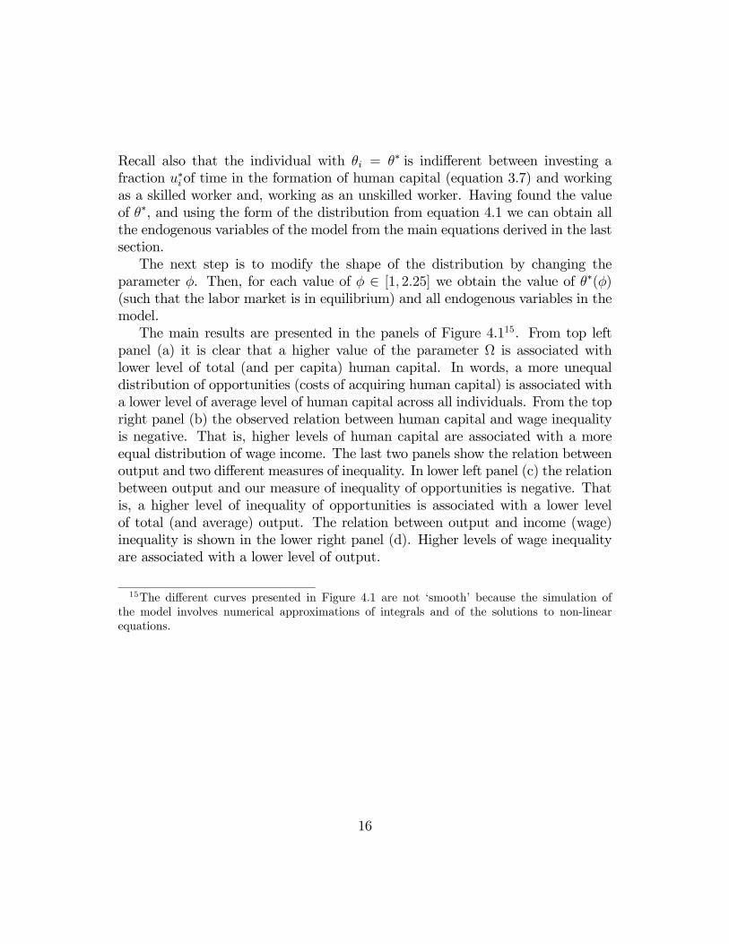
Recall also that the individual with θi = θ∗ is indifferent between investing afraction u∗i of time in the formation of human capital (equation 3.7) and workingas a skilled worker and, working as an unskilled worker. Having found the valueof θ∗, and using the form of the distribution from equation 4.1 we can obtain allthe endogenous variables of the model from the main equations derived in the lastsection.The next step is to modify the shape of the distribution by changing the

parameter φ. Then, for each value of φ ∈ [1, 2.25] we obtain the value of θ∗(φ)(such that the labor market is in equilibrium) and all endogenous variables in themodel.The main results are presented in the panels of Figure 4.115. From top left

panel (a) it is clear that a higher value of the parameter Ω is associated withlower level of total (and per capita) human capital. In words, a more unequaldistribution of opportunities (costs of acquiring human capital) is associated witha lower level of average level of human capital across all individuals. From the topright panel (b) the observed relation between human capital and wage inequalityis negative. That is, higher levels of human capital are associated with a moreequal distribution of wage income. The last two panels show the relation betweenoutput and two different measures of inequality. In lower left panel (c) the relationbetween output and our measure of inequality of opportunities is negative. Thatis, a higher level of inequality of opportunities is associated with a lower levelof total (and average) output. The relation between output and income (wage)inequality is shown in the lower right panel (d). Higher levels of wage inequalityare associated with a lower level of output.

15The different curves presented in Figure 4.1 are not ‘smooth’ because the simulation ofthe model involves numerical approximations of integrals and of the solutions to non-linearequations.

16

Figure 4.1:

17

5. Conclusions

The paper develops an heterogeneous agent general equilibrium model with un-equal opportunities of access to the educational system. More precisely, we specifyinequality of opportunities among individuals as a differential cost of access to theeducational process. In equilibrium, the endogenous variables of the model aredetermined by the form of the distribution of costs across individuals as well asthe parameters of the technologies of production of the final good and human cap-ital formation. In order to study the relation between the endogenous variablesof the model we do a numerical simulation of the model using a well behaved (forour main purposes) distribution function of the costs of acquiring human capital.More precisely, we find a negative relation between inequality of opportunitiesand income and two different measures of efficiency (output per capita and hu-man capital per capita). An additional exercise (not presented in this version ofthe paper) uses a different distribution function and the main results regardingthe trade-off between efficiency and equality are maintained16. Although the dis-tribution used in the paper for the simulation is very particular, it is a tractableone in the sense that it allows to isolate changes in the shape (dispersion) of thedistribution from changes in the mean. We are aware that this distribution isone of the many possible distributions that we can observe in reality. Furtherwork will focus on the identification of the sufficient and necessary conditions onthe distribution function for the trade-off between equality of opportunity andefficiency in the formation of human capital to exist.16These results are available from the authors upon request.

18

ReferencesAngrist, J., Bettinger, E., Bloom, E., Kling, E., and M. Kremer,

2003, “Vouchers for Private Schooling in Colombia: Evidence from a RandomizedNatural Experiment”, American Economic Review,Bénabou, R., 1996, “Equity and Efficiency in Human Capital Investment:

The Local Connection”, Review of Economic Studies, 62, 237-264.Bénabou, R., 2000, “Meritocracy, Redistribution, and the Size of the Pie”,

in Arrow et al. Meritocracy and Economic Inequality, Princeton UniversityPress.Banerjee, A.V. and A.F. Newman, 1993, ”Occupational Choice and the

Process of Development”, Journal of Political Economy, 101(2): 274-298.Betts, J. and D. Morell, 1999, “The Determinants of Undergraduates

Grade Point Average: The relative Importance of Family Background, High SchoolResources, and Peer group Effects”, Journal of Human Resources, 34, 2, 268-293.Dardanoni, V., G. Fields, P. Roemer and M. Sanchez, 2003, “How

demanding should equality of opportunity be, and how much have we achieved”,unpublished manuscript.De Gregorio, J., 1996, ”Borrowing constraints, human capital accumula-

tion, and growth”, Journal of Monetary Economics 37, 49-71.Duflo, E. and M. Kremer, 2003, “Use of Randomization in the Evaluation

of Development Effectiveness”, mimeo, MIT.Durlauf, S., 1996, “Neighborhood Feedbacks, Endogenous Stratification,

and Income Inequality”, in: Barnett, Gandolfo, and Hillinger eds., Dynamic Dis-equilibrium Modelling, Cambridge, Cambridge university Press.Durlauf, S., 2002, “Groups, Social Influences and Inequality: A Membership

Theory Perspective on Poverty Traps”, University of Wisconsin..Fernandez, R. and Rogerson, 1996, “Keeping People Out: Income Dis-

tribution, Zoning, and the Quality of Public Education”, Quarterly Journal ofEconomics, 38, 1, 25-42.Flug, K, A. Spilimbergo and E. Wachteinheim, 1998, ”Investment in

education: do economic volatility and credit constraints matter?” Journal ofDevelopment Economics 55, 465-481.Galor, O. and J. Zeira, 1993, ”Income Distribution and Macroeconomics”,

Review of Economic Studies, 60: 35-52.

19

Galor, O. and D. Tsiddon, 1997, “Technological Progress, Mobility, andEconomic Growth”, American Economic Review, Vol. 87, No. 3, 363-382.Ginther, D., R. Haveman and B.Wolfe, 2000, “Neighborhood Attributes

as Determinants of Children’s Outcomes: How Robust are the Relationships”,Journal of Human Resources, Vol. 35, No. 4, 603-642.Goldhaber, D. and D. Brewer, 1997, “Why don’t Schools and Teachers

Seem to Matter? assessing the Impacts of Unobservables on Educational Produc-tivity”, Journal of Human Resources, 32, 3, 505-523.Grogger, G., 1997, “Local Violence and Educational Attainment”, Journal

of Human Resources, 32, 4, 659-682.Hanushek, E., 1986, “The Economics of Schooling: Production and Ef-

ficiency in Public Schools”, Journal of Economic Literature, vol. 24, No. 3,1141-1177.Hanushek, E., 1996, “Measuring Investment in Education”, Journal of Eco-

nomic Perspectives, Vol. 10, No. 4, 9-30.Kremer, M., 2003, “Randomized Evaluation of Educational Programs in

developing Countries: Some Lessons, forthcoming in American Economic Reviewpapers and proceedings..Roemer, J., 2000, “Equality of Opportunity”, in Arrow et al. Meritocracy

and Economic Inequality, Princeton University Press.Schultz, T. Paul, “School Subsidies for the Poor: Evaluating the Mexican

Progresa Poverty Program”, Journal of Development Economics, forthcoming.Thomas, V., Y. Wang and X. Fan, 2000, “Measuring Education Inequal-

ity: Gini Coefficients of Education”, World Bank.

20

Appendix

(a)Note that from equation 3.7, b(u∗i ) =

³γ

θi(1+γ)

´γdenotes the level of human

capital at the optimum for individual i. Recall that θi is different for all individualsand determines the extra cost of acquiring human capital based on socioeconomiccharacteristics. Let, only as an example, these set of costs be determined by aweighted average17 of two characteristics: the inverse of parent’s level of educa-tion (εi) and an inverse measure of health (κi) . That is: θi = δελi κ1−λi , with λunknown. If parents level of education and health characteristics are observed foreach individual and we are able to proxy b(u∗i ) with test scores or an indicator ofyears of schooling for each individual (si) then, the effects of parents educationand health can be estimated from the log-linearization of the optimal amount ofhuman capital derived above. That is:

ln si = γ lnγ

δ (1 + γ)− γλ ln εi − γ(1− λ) lnκi.

From the estimation of the above equation, a researcher can estimate the effectsof different characteristics of the individual on observed educational outcomes. Inmany of the empirical studies reviewed in the introduction this is the form thatis estimated.17It is not necessary that the weights add up to 1, but is a hypothesis that can be tested.

21

(b)

Source: Thomas et al. (2000)

Education Lorenz Curve, India 1960

0.0

75.7

0.0

100.0

96.6100.0

0.0

37.2

95.5

0

20

40

60

80

100

0 20 40 60 80 100Cumulative Proportion of Population Distribution

(%)

Cum

ulat

ive

Prop

ortio

n of

Sch

oolin

g (%

)

Q

PO

S

Mean=1.09 yearsEducation Gini = .79

Education Lorenz Curve, Korea 1960

0.0

48.2

0.0

68.7

2.70.0

94.490.3

100.0

0

20

40

60

80

100


(%)

Cum

ulat

ive

Prop

ortio

n of

Sch

oolin

g(%

)

Q

PO

S


Education Lorenz Curve, India 1990

0.0

23.8

0.0

100.0

83.8

91.0

0.0

10.9

63.3

0

20

40

60

80

100


(%)

Cum

ulat

ive

Prop

ortio

n of

Sch

oolin

g (%

)

Q

PO

S


Education Lorenz Curve, Korea 1990

0.09.4

24.9

0.20.0

89.2

78.3

100.0

0

20

40

60

80

100


(%)

Cum

ulat

ive

Prop

ortio

n of

Sch

oolin

g (%

)

Q

PO

S


Figure 5.1:

22

Source: Thomas et al. (2000)

Average years of schooling and Education Gini

0

2

4

6

8

10

12

14

0.0000 0.2000 0.4000 0.6000 0.8000 1.0000

Education Gini

Avg

. yea

rs o

f sch

oolin

g (p

op. o

f age

15

and

over

Figure 5.2:

23

unequal opportunities and human capital formation€¦ · · 2009-09-22unequal opportunities and...

Documents