unequal probability-based spatial sampling arcuser article - esri

10 au Spring 2013 esri.com

The geographic approach involves measuring the earth, organizing the resultant data, and analyzing it to understand spatial processes and relationships. GIS technologies are used extensively for the latter stages of the geographic approach but less often for sampling, an important component of measurement. This article shows how to use ArcGIS 10 for Desktop to create an efficient spatial sampling or suitability design using the Create Spatially Balanced Points geoprocessing tool available with the ArcGIS Geostatistical Analyst extension and other geoprocessing tools provided with the core product.

Unequal Probability-Based

SpatialSampling

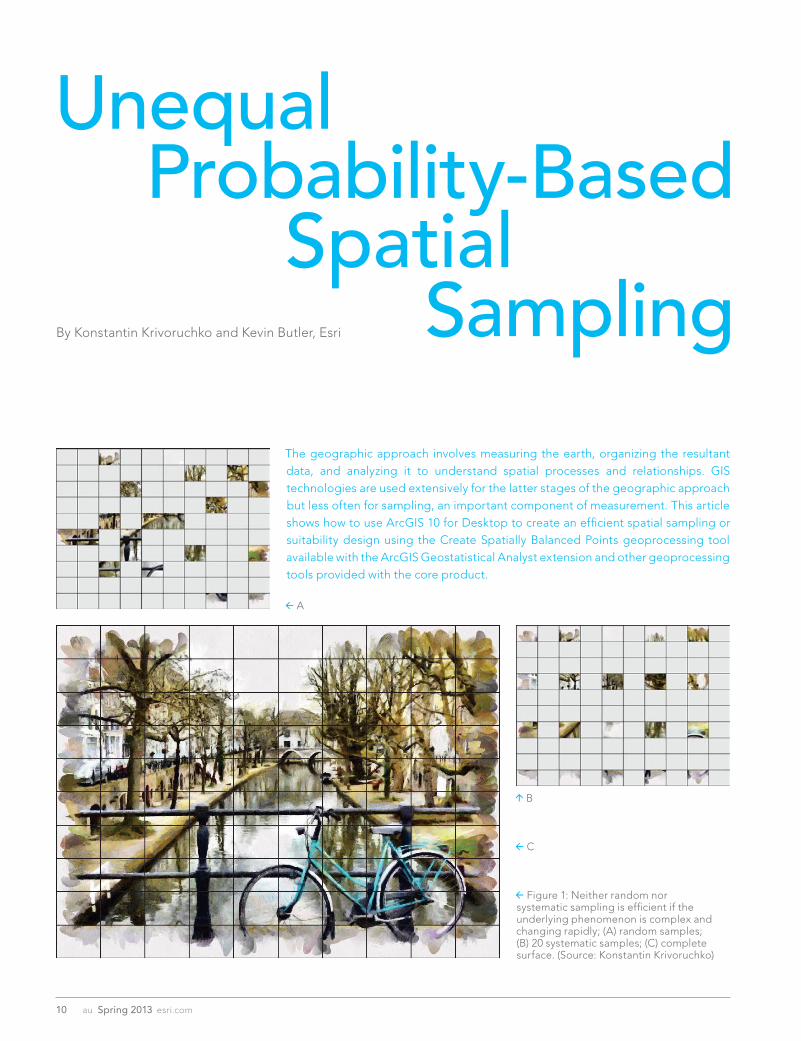
Figure 1: Neither random nor systematic sampling is efficient if the underlying phenomenon is complex and changing rapidly; (A) random samples; (B) 20 systematic samples; (C) complete surface. (Source: Konstantin Krivoruchko)

By Konstantin Krivoruchko and Kevin Butler, Esri

A

B

C

11esri.com Spring 2013 au

Figure 2b: 3D view showing lack of smoothness in averaged data

Software and Data

Scientists synthesize knowledge through the process of collecting and classifying empirical data (i.e., samples) with the ultimate goal of generalizing their observations, through inductive reasoning, into universal laws. The laws are required to make inference from the ob-served to the unobserved data. However, Immanuel Kant showed that empirical observations alone cannot lead to universal knowledge (although the knowledge that universal knowledge actually exists) but must be tempered by what researchers believe is the appropriate conceptual description of reality. This is independent of observational knowledge that exists in the researcher’s mind and helps make sense of empirical data. Kant called this type of knowledge a priori knowledge. This article describes a workflow for collecting a relatively small number of samples to reconstruct an unobserved or partially ob-served spatial variable with reasonable uncertainty using a priori knowledge about the phenomenon under study. The set of geographic locations where measurements are taken is called a spatial sampling design. An efficient sampling design specifies sampling locations that allow the researcher to confidently estimate the value of the sampled variable, such as pollution, at unsampled locations. The workflow for developing a probability-based spatial sampling design that balances the conflicting goals of maintaining high prediction accuracy and minimizing cost and

Figure 2a: Ohio air pollution data aggregated to 75 random polygons

Figure 2c: Averaged data smoothed using areal interpolation47–6,162

6,163–18,983

18,984–50,192

50,193–106,954

106,955–165,490

Air Pollution Site

Aggregated Air Pollution (pounds)

47–1,296

1,296–5,140

5,140–16,971

16,971–53,390

53,390–165,490

Aggregated Air Pollution (pounds)

w w w. e x t e n s i o n . u c r . e d u / e s r i

• Project Based Curriculum

• Field Trips & Tours

• Networking Events

• Software Training

17th AnnuAl

GIS Summer School

July-August summer 2013


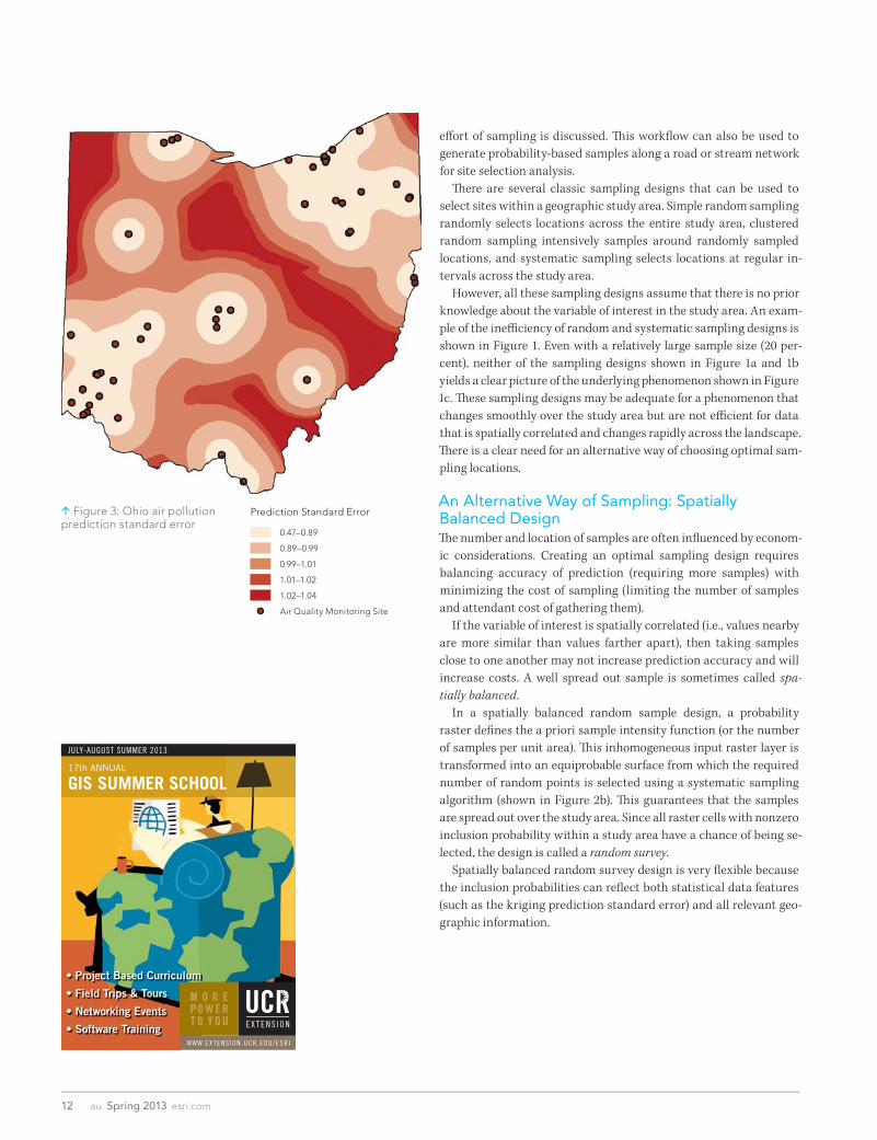
Figure 3: Ohio air pollution prediction standard error

0.47–0.89

0.89–0.99

0.99–1.01

1.01–1.02

1.02–1.04

Air Quality Monitoring Site

Prediction Standard Error

eff ort of sampling is discussed. Th is workfl ow can also be used to generate probability-based samples along a road or stream network for site selection analysis. Th ere are several classic sampling designs that can be used to select sites within a geographic study area. Simple random sampling randomly selects locations across the entire study area, clustered random sampling intensively samples around randomly sampled locations, and systematic sampling selects locations at regular in-tervals across the study area. However, all these sampling designs assume that there is no prior knowledge about the variable of interest in the study area. An exam-ple of the ineffi ciency of random and systematic sampling designs is shown in Figure 1. Even with a relatively large sample size (20 per-cent), neither of the sampling designs shown in Figure 1a and 1b yields a clear picture of the underlying phenomenon shown in Figure 1c. Th ese sampling designs may be adequate for a phenomenon that changes smoothly over the study area but are not effi cient for data that is spatially correlated and changes rapidly across the landscape. Th ere is a clear need for an alternative way of choosing optimal sam-pling locations.

An Alternative Way of Sampling: Spatially Balanced DesignTh e number and location of samples are often infl uenced by econom-ic considerations. Creating an optimal sampling design requires balancing accuracy of prediction (requiring more samples) with minimizing the cost of sampling (limiting the number of samples and attendant cost of gathering them). If the variable of interest is spatially correlated (i.e., values nearby are more similar than values farther apart), then taking samples close to one another may not increase prediction accuracy and will increase costs. A well spread out sample is sometimes called spa-tially balanced. In a spatially balanced random sample design, a probability raster defi nes the a priori sample intensity function (or the number of samples per unit area). Th is inhomogeneous input raster layer is transformed into an equiprobable surface from which the required number of random points is selected using a systematic sampling algorithm (shown in Figure 2b). Th is guarantees that the samples are spread out over the study area. Since all raster cells with nonzero inclusion probability within a study area have a chance of being se-lected, the design is called a random survey. Spatially balanced random survey design is very fl exible because the inclusion probabilities can refl ect both statistical data features (such as the kriging prediction standard error) and all relevant geo-graphic information.

Distance from Road (feet)

0 1000.00

0.25

0.50

0.75

1.00

200 300 400

Suit

abili

ty

1+exp –2 *

1

( (30x–300


Figure 4a: Sigmoidal function used to rescale distance from road to suitability score

Figure 4b: Example of roads suitability surface in Summit County, Ohio

0–0.001

0.002–0.013

0.014–0.107

0.895–0.989

0.108–0.894

0.99–1

Creating a Sampling Design for Measuring Pollution Deposition Like many Midwestern counties, Summit County, Ohio, is located in a region where there is signifi cant manufacturing activity and coal power generation still takes place. Th e county has high population density and is bisected by seven major state and interstate highways. Th ese factors suggest a need to accurately monitor the levels of at-mospheric pollution deposition across the county. Data from Summit County will be used to demonstrate how to construct an a priori probability surface to select optimal sampling locations. Considerations in creating the a priori probability surface include estimating total air pollution from known pollution sources, predicting uncertainty of current air pollution measurements, and using best practices for selecting undisturbed sampling locations. Th e overall goal of the design is to select locations in the county that h ave both a high level of atmospheric pollution and a high level of prediction uncertainty from the existing air pollution monitoring network yet are located in undisturbed areas so measurements will be useful for environmental modeling.

Estimating Distribution of Air Pollution from Known Pollution SitesTh e US Environmental Protection Agency (EPA) maintains a data-base of the release of toxins to the air, water, and land called the Toxic Release Inventory (TRI) (www.epa.gov/tri/). Th e amount of pollution released to the air from 3,448 pollution sites in the state of Ohio was downloaded from the TRI database. Even though this workfl ow will select sampling sites only in Summit County, air pollu-tion distribution should be estimated for the entire state to mitigate the external boundary problem common in ecological analysis. An estimate of the air pollution levels across the state could be immediately created using one of the kriging models, but this would be inappropriate given that pollutants were released in diff erent amounts, at diff erent times of the year, and under diff erent weather conditions. Some preprocessing of the data is necessary before it can be transformed into a prediction surface. Averaging the data to a suffi ciently large number of random polygons and smoothing using a polygon-based interpolator can be done using geoprocessing tools in ArcGIS for Desktop. Use the Create Random Points tool (Data Management toolbox) to generate 75 random points within the broader study area. Th is number is suffi cient for use in kriging. Use the Minimum Allowed Distance parameter to ensure points are spread out across the study area.

Software and Data


Figure 5a: Ten spatially balanced candidate sites in Summit County, Ohio

Probability of Selection

Hig

h: 1

Low

: 0

Generate Thiessen polygons around each of the 75 random points using the Create Thiessen Polygons tool (Analysis toolbox > Proximity toolset). Spatially join and average the air pollution data to the Thiessen polygons using the Joins and Relates dialog box accessed from ArcMap’s table of contents (Figure 2a). Figure 2b shows a 3D representation of the pollution data aggre-gated to polygons. Geostatistical Analyst has a kriging model called areal interpolation, which has been designed specifically for data that has been averaged over polygons. Given the Thiessen polygons and the average air pollution estimates, a prediction surface is pro-duced for all points in the study area (Figure 2c). This surface will serve as a smooth approximation of the industrial air contamination.

Determining Uncertainty of Existing Air Pollution MeasurementsThe US EPA maintains a database of air quality measurements taken throughout the United States and its territories (www.epa.gov/airdata/index.html). Data on particulate matter (i.e., matter 2.5 mi-crometers and smaller in diameter) was extracted for the 46 moni-toring sites located in Ohio. These measurements serve as a proxy for estimating the uncertainty in the existing air pollution monitoring system. One goal of the sampling design is to take new samples in areas where the uncertainty of prediction from existing measurements is high. Using the values from the 46 monitoring sites in Ohio, a predic-tion surface and standard error of prediction surface was created for the state using empirical Bayesian kriging. This tool was selected because it requires minimal interactive modeling and its standard errors of prediction are more accurate than standard errors of pre-diction from other kriging models. Darker areas of Figure 3 show higher levels of uncertainty of air pollution prediction.

Sampling in Undisturbed AreasBecause this study is looking at cumulative deposition of pollution, it is important to avoid taking samples too close to roads because road traffic resuspends particles, creating what is known as fugitive dust. The US EPA recommends siting air pollution and deposition moni-toring sites in flat, uniform, and open spaces at least 200 meters (m) from a lightly traveled secondary road, 500 m from a heavily traveled secondary road, or 2 kilometers from a major highway. However, in an urban county, such as Summit County, which has a dense road network, these parameters would exclude most of the county. As a compromise, the Euclidean distance to the nearest road was calculated, and the distances were rescaled using a sigmoi-dal function shown in Figure 4a. The effect of this function is that locations close to a road (0–50 m) will have a very low suitability. Once the distance from a road reaches 50 m, suitability begins to gradually increase. When the distance reaches approximately 250 m, suitability levels off and all distances greater than this distance are nearly equally preferred (as shown in Figure 4b).


Putting It All TogetherEach of the three rasters generated from this workflow represents a goal of the sampling design. To consider all three goals at the same time, the rasters must be rescaled and combined. Rescaling trans-forms the rasters to a common measurement scale so that they will have equal influence in the site selection. Rasters were transformed to a 0 to 1 scale using the formula (raster value - minimum raster value)/(maximum raster value - raster min). rasters were combined using the formula (pollution raster + predic-tion uncertainty raster) * roads raster. Multiplying by the roads layer (where locations close to the road have very low suitability scores) dramatically reduces the final suitability for locations close to a road. The combined raster is a surface where higher values represent more desirable locations for sampling. This final raster was also rescaled to a 0 to 1 scale to represent a probability range. The higher the value in this raster, the more likely that the cell will be included in the sample design. In this example, the pollution and prediction uncertainty rasters were considered equally important in determin-ing site suitability, so they were simply added together. However, more importance could be assigned to one of the factors by multi-plying it by a weight before adding the rasters together. Figures 5a and 5b show the resultant inclusion probability raster and two sets of candidate sample sites. Note that each sample reali-zation is related to the underlying spatial structure of the sampling suitability raster created earlier. The samples are also spatially bal-anced. If Thiessen polygons were drawn around each sample loca-tion, all polygons would have somewhat similar areas.

Other Applications of the WorkflowThis workflow can be used for other applications such as locating sampling sites along a stream or road network, which is often a difficult task in GIS. Using the Feature To Raster tool (Conversion toolbox), the road or stream network can be converted to a raster, and locations on the stream or road can be assigned a value of 1 and all other locations assigned a value of 0. Using this raster as input to the Create Spatially Balanced Points geoprocessing tool results in a random sample of points along the network (Figure 6a). Alternatively, locations along the stream or road could be given higher inclusion probabilities based on proximity to features such as dams or envi-ronmentally sensitive areas. Raster-based site selection is one of the most common workflows in GIS. In this method, raster layers are rated, weighted, and over-laid to create a final suitability raster. These analyses are often per-formed at fine raster resolutions using 30 m cells to capture rapidly changing criteria such as elevation or land use. This can result in a

“salt and pepper” effect on the suitability raster that contains several isolated cells with high suitability values (Figure 6b). To locate potential sites for three new large sporting goods stores, for example, individual cells of approximately 0.2 acres each (shown in Figure 6b) would be too small to site such large facilities. To solve this problem would require resampling the final suitability

Software and Data

Figure 5b: Thirty spatially balanced candidate sites in Summit County, Ohio

Probability of Selection

Hig

h: 1

Low

: 0


raster to a cell size appropriate for the facility being sited. Figure 6c shows the suitability raster resampled to a 5-acre cell size. After rescaling this raster to a 0 to 1 scale, it can be used as input to the Create Spatially Balanced Points tool. Figure 6c shows potential sites for three stores. These sites are spatially balanced and were se-lected based on their suitability. The Thiessen polygons around each of the sites can be thought of as the catchment area for each store.

ConclusionUnequal probability-based sampling using the Create Spatially Balanced Points tool allows the researcher to use a priori knowledge of a problem to create an intelligent and efficient sampling or suit-ability design. The tool uses continuously varying inclusion proba-bilities that can be readily constructed using a variety of geographic layers and the researcher’s expert knowledge. This powerful, flexible, and easy-to-use tool can lead to a reduction in the cost and effort of sampling designs used to evaluate patterns and trends in geograph-ic data. For more information on creating spatially balanced points, see the resources listed under Further Reading.

Figure 6c: Suitability raster resampled to approximately 5-acre cell size. Stars represent potential store locations. Polygons represent store catchment areas. Darker colors indicate higher suitability.

Figure 6a: Fifteen spatially balanced sampling locations selected along a sinuous river. All locations along the stream are equally probable.

Figure 6b: Suitability raster for siting a large sporting goods store. Notice several isolated cells, which have high suitability but are not large enough to site a store. Darker colors indicate higher suitability.

Geospatial Education Portfolio

Enroll in one of our high-quality online education programs to help you achieve your career goals:

Master of Geographic Information Systems Master of GIS—Geospatial Intelligence Option Postbaccalaureate Certificate in GIS Graduate Certificate in Geospatial Intelligence

P e n n S t a t e | O n l i n e

U.Ed.OUT 13-0349/13-WC-0334ajp/sss

www.worldcampus.psu.edu/ArcUser13


Software and Data

Further ReadingArcGIS Help 10.1. Create Spatially Balanced Points (Geostatistical Analyst). Krivoruchko, Konstantin. “Empirical Bayesian Kriging,” ArcUser, Fall 2012, p. 6. Krivoruchko, Konstantin. “Modeling Contamination Using Empirical Bayesian Kriging.” ArcUser Online, Fall 2012 (esri.com/news/arcuser/1012/modeling-contamination-using-empirical-bayesian-kriging.html).Krivoruchko, Konstantin. Spatial Statistical Data Analysis for GIS Users. Esri Press, 2011, 928 pp.Krivoruchko, Konstantin, A. Gribov, and E. Krause. 2011.

“Multivariate Areal Interpolation for Continuous and Count Data.” Procedia Environmental Sciences, Vol. 3, pp. 14–19. 1st Conference on Spatial Statistics 2011—Mapping Global Change.Stevens, D. L., Jr., and A. R. Olsen. 2004. “Spatially Balanced Sampling of Natural Resources.” Journal of the American Statistical Association 99 No. 465: 262–278.

About the AuthorsKonstantin Krivoruchko is a senior research associate on the Esri software development team who played a central role in developing the ArcGIS Geostatistical Analyst extension. Prior to joining Esri in 1998, he was director of the GIS laboratory at the Sakharov Institute of Radioecology in Minsk, Belarus, where he developed GIS and spa-tial statistics curricula and supervised doctoral and graduate school candidate research pertaining to GIS applications and spatial statis-tical data analysis. He has taught numerous courses on applied spa-tial statistics and GIS. These activities are summarized in the book Spatial Statistical Data Analysis for GIS Users, published by Esri Press.

Kevin Butler is a member of the Spatial Analyst team working pri-marily with the multidimension tools. He holds a doctorate in geog-raphy from Kent State University. Prior to joining Esri last year, he was a senior lecturer and the manager of GIScience research at the University of Akron, where he taught courses on spatial statistics, GIS programming, and database design.

unequal probability-based spatial sampling arcuser article - esri

Documents