Unilateral Practices, Antitrust Enforcement andCommitments

Michele PoloBocconi University, IGIER and IEFE

Patrick ReyToulouse School of Economics

February 2016Preliminary and incomplete, please do not quote or circulate

AbstractThis paper analyses the optimal setting of remedies and commitments

in antitrust enforcement against unilateral practices, a tool introduced withthe Modernization reform in 2003 that is now intensively used both by theEuropean Commission and the National Antitrust Authorities. We modelthe issue as a signalling game where nature determines whether a prac-tice is socially harmful or beneficial, the firm offers a commitment andthe Authroity decides whether to accept it or to run a costly investigationcollecting hard evidence with positive probability. We show that commit-ments should be used in more harmful cases where the Competition author-ity hardly finds evidence. However, since commitments are accepted oncethe action is undertaken, the authority accepts them too often disregardingtheir effects of weakening deterrence

Keywords: Antitrust enforcement, commitment, remedies, deterrence

1 Introduction

The modernization reform in 2003 has introduced some new tools that the com-petition autorities (CA) can use in prosecuting unilateral practices. Firms thatare involved in a case can offer commitments that, if accepted by the CA, becomecompulsory remedies. Commitments usually refer to adopting, or abstainingfrom adopting, certain practices, and are intended to limit the anticompetitiveeffects of the firm’s behavior, restoring competition. While appealing to shortena case and save resources, thereby obtaining practical effects in the market, com-mitments are offered and accepted while the CA has not a full understandingof the effects of the practices involved. Hence, the firm can exploit its supe-rior information. The incentive of the CA to accept the commitments, in turn,rests on the possibility of saving time and resources, closing the case in a shortdeadline and with some practical effects at work.

1

After the introduction of regulation 1/2003, the European Commission andthe national CA have increasingly relied on commitments1 , raising a debateon the opportunity of such a widespread adoption. Those that have a criticalview on this tool suggest that they create an incentive for firms to attemptdubious practices, having the escape way of offering commitment if the CAopens the case, thereby waiving the fines. The ultimate effect, then shouldbe that of weakening deterrence. On the opposite side, those in favor of thisnew instrument claim that commitments dramatically shorten the duration ofantitrust case and deliver a certain and ready result, as compared to long,costly and uncertain outcomes if the case is run until the final decision and thefollowing judicial review.Although commitments are today a very common tool, surprisingly there is

no theoretical analysis, to the best of our knowledge, to frame the problem intoa model that allows delivering answers regarding the optimal way to admin-ister commitments. In this paper we propose a signalling game where naturedetermines whether a practice is socially harmful or beneficial, the firm offers acommitment and the authority decides whether to accept it and close the caseor run a full investigation, collecting costly information and obtaining evidencewith a positive probability. In this latter case, it levies a fine and imposesremedies on the firm.We show that commitments should be used only when the practice is pre-

sumably socially harmful, when it is particularly damaging and when gatheringinformation is hard. By offering commitments the firm cashes in, as retainedextra profits, the saving in costs from accepting the commitments and clos-ing the case after a short period. The effi ciency in enforcement, in turn, mustbe traded off with the increased incentives to undertake practices even whensocially harmful, the weakening deterrence effect.The paper is organized as follows: section 2 presents the set up, section 3

starts the analysis. Section 4 considers the case of costly investigation, sec-tion 5 compares the outcomes with the case when commitments are banned.Conclusions follow. All the proofs are in the Appendix.

2 Set-up

In line with the rules introduced with Regulation 1/2003, and in particular art.7 and 9, we analyze the enforcement of art. 102 against the abuse of a dominantposition. If the competition authority (CA) has stated its competitive concernin the Statement of Objection at the end of the first phase of the procedure, thefirm may submit commitments. Ig the CA accepts them, they become bindingand the authority closes the case with no infringement decision. If, however,the authority rejects the commitments, the procedure continues. If the CA does

1 In the period 2004-2013 out of 47 art.102 cases at the European Commission 27 of themwhere closed with commitments and without issueing a decision of antitrust violation..

2

not prove the infringement, it clears the case, whereas if the CA collects hardevidence of the illegal behavior, it fines the firm and obliges it to undertakeremedies that affect both the private and social effects of the practice.

More formally, the setting we analyze is described as follows.

Stage 0

i) The legislator defines the policy tools available to the competition author-ity (CA), that determine the possible outcomes of a case: the CA candecide to close the case after a quick review; it can decide tu run a fullinvestigation that entails more time and resources, at the end of whichit can convict the firm only if it obtains hard evidence that the practiceis welfare decreasing (anticompetitive). In this latter case the CA has toimpose a fine F > 0 and a remedy R. Finally the CA can accept com-mitments that the firm offers once a case is opened, turning them intocompulsory remedies.

ii) Nature draws the firm’s type θ ∈ {G,B}, that is whether the actionthe firm may undertake (a business practice) is bad (welfare decreas-ing/anticompetitive) (B) or good (welfare enhancing/competitive) (G),with Pr(θ = G) = λ ∈ (0, 1). The firm knows its type θ while the CAdoes not observe the firm’s type and only knows the ex-ante probabilityλ.

iii) The type-θ firm decides to undertake the action with probability αθ ∈[0, 1] and gains gross profits Πθ = Π. If it acts, it bears the cost γ, that isuniformely distributed in [0,Π] independently of the firm’s type θ. Whenthe type is good (θ = G) the social effects of the practice are positive, i.e.WG = W > 0, while when the type is bad (θ = B), private and socialeffects diverge, since WB = −L, with L > 0 being the social loss.

iv) The CA observes that a firm is acting and updates its prior λ to λ0 accordingto the equilibrium probabilities αθ that the θ firm acts. Then, the CAdecides whether to open the case (δ0 = 1) or not (δ0 = 0). We assumethat if the expected welfare in the two options is the same, the CA doesnot open the case2

Stage 1

i) If the case is opened, the firm offers a commitment C.

ii) The CA decides whether

R1 = C : to accept the commitment and transform it into a remedy,such that Πθ(R1 = C) = (1− C)Π and Wθ(R1 = C) = (1− C)Wθ,

2We could assume, alternatively, that opening the case entails some (negligible) initialadministrative cost kA0 , introducing a further parameter.. In order to streamline the analysiswe prefer to simply assume this (reasonable) tie-breaking rule.

3

R1 = 0 : to close the case, yielding payoffsΠθ(R1 = 0) = Π andWθ(R1 =0) = Wθ

δ1 = 1 : to move to stage 2.

Stage 2

i) If the authority decides to move to stage 2, then it bears a cost kA2 and thefirm a cost kF2 related to the administrative and legal process. We definek2 = kA2 + kF2 as the private and public cost of a full investigation. TheCA receives a signal σ ∈ {θ, ∅} on the firm’s type θ. The signal revealshard (verifiable) information on the firm’s type with probability ρ ∈ (0, 1)and no information with probability 1− ρ.

ii) At the end of the procedure, the CA either closes the case (R2 = F2 = 0)or imposes a remedy R2 ∈ (0, 1] and a fine F2 ∈ {0, F}, such thatΠθ(R2, F2) = (1 − R2)Π − F2 and Wθ(R2) = (1 − R2)Wθ. The CAcan convict the firm at the end of the procedure only if it collects hardinformation that the practice is welfare decreasing, i.e. if σ = B.

Hence, our set-up aims at capturing in the simplest way the main ingredi-ents of the adoption of commitments: the CA has initially a limited evidenceof the case, as represented by the probability λ that the practice is anticompet-itive. If it decides to open the case, then the authority faces two alternatives.It may accept the commitment offered by the firm, thereby closing the case.Alternatively, the authority may reject the commitment and proceed with a fullinvestigation, hoping to collect decisive evidence although bearing additionalcosts.In our setting the regulation gives the Authority the possibility of accepting

commitments once the case has been opened. This implies that the Authoritydecides ex-post, after the practice has been undertaken and the case opened,whether to accept commitments or not. This feature, that reflects the provi-sions of the European regulation, plays a key role on the overall impact of theenforcement policy, and specifically on its effectiveness on ex-ante deterrence.

3 Analysis

3.1 Beliefs and updating

If the firm receives at time t = 2 an informative signal σ = θ, it updates itsbeliefs accordingly. If, instead, the signal is uninformative no updating occurs,since in stage 2 the firm does not take any action that may signal its type. Letus denote

λ2(σ) =

1 if σ = Gλ1 if σ = ∅0 if σ = B

, (1)

4

where λ1 if the posterior probability that the practice is welfare enhancing attime 1.At time t = 1 the firm offers a commitment C that may act as a signal of its

type. In a Perfect Bayesian Equilibrium (PBE), then, the CA updates its beliefson the firm’s type based on the equilibrium choices of a type-θ firm, as long asthe observed choice is in the equilibrium set. In a (candidate) separating PBEin which C∗G 6= C∗B , if at time 1 the CA observes the equilibrium strategy of thegood type, then it updates its belief to λ1(C∗G) = 1, whereas the posterior isλ1(C∗B) = 0 after observing the equilibrium choice of the bad type. If the PBE,instead, is pooling, i.e. C∗G = C∗B , the beliefs do not change when observing anequilibrium choice, i.e. λ1 = λ0.Finally, at time t = 0 the CA updates its beliefs upon observing the action

based on the equilibrium probabilities α∗θ that a θ-type firm decides to undertakethe action, according to the Bayes rule:

λ0 =λα∗G

λα∗G + (1− λ)α∗B

where λ is the prior probability of the good state.Moreover, we assume the CA adopts passive beliefs after observing an out-

of-equilibrium choice at time t: the CA believes that both types have chosenthe out-ot-equilibrium action with the same probability, and therefore, applyingthe Bayes rule, λt = λt−1.

3.2 Optimal policies

Let us construct the expected welfare and the optimal decision rule of the CAmoving backward and starting from t = 2. Phase 2 is reached if the CA opensthe case (δ0 = 1) and if, at t = 1, it does not close the case (R1 = 0) nor acceptsthe commitment (R1 = C). The expected welfare at t = 2, then, depends onthe beliefs (1) and the policy R2(λ2(σ)) adopted:

EW2(λ2(σ)) = λ2(σ) (1−R2(λ2(σ)))W − (1− λ2(σ)) (1−R2(λ2(σ)))L− k2.

Taking into account that the CA cannot convict the firm if it does not collecthard evidence of a negative welfare effect, the optimal policy at stage 2 is:

R∗2(σ) =

R2 = 0 if σ = GR2 = 0 if σ = ∅R2 = 1 if σ = B

.

At t = 1, the policy options to consider are: the CA can close the case(R1 = 0), accept the commitment (R1 = C) or move to stage 2 (δ1 = 1). Giventhe posterior λ1 at stage 1, the expected welfare in the three cases is:

EW1(R1 = 0) = λ1W − (1− λ1)L ≡ EW1 (2)

EW1(R1 = C) = (1− C)EW1

EW1(δ1 = 1) = EW1 + (1− λ1)ρL− k2.

5

Notice that the expected welfare when moving to stage 2 instead of closingthe case involves two effects: a positive one ((1 − λ1)ρL), that derives fromavoiding the welfare loss if the signal is informative and, indeed, the action isanticompetitive, and a negative one, related to the costs of the authority andthe firm when running a full investigation, k2.When λ1 = 0, we have 0 > EW1(δ1 = 1) = −(1 − ρ)L − k2 > EW1(R1 =

0) = −L if k2 < ρL. Moreover, 0 < ∂EW1(δ1=1)∂λ1

= W+(1−ρ)L < ∂EW1(R1=0)∂λ1

=W+L. Indeed, when the CA becomes marginally more optimistic, i.e. λ1 ↑, if itcloses the case (R1 = 0) the expected welfare increases because the welfare gainW (welfare losses L) becomes more (less) likely. When, instead, the CA proceedsto stage 2, the welfare loss occurs only when the signal is uninformative, an eventthat realizes with probability 1− ρ. Consequently, the avoided loss under moreoptimistic beliefs is (1 − ρ)L. In turn, when the CA accepts the commitment∂EW1(R1=C)

∂λ1= (1 − C) (W + L): when the beliefs become marginally more

optimistic both the welfare gain an the avoided loss become smaller due tocommitments.Having identified the payoffs in the different policy outcomes we can now

establish a preliminary result that excludes the possibility of a separating equi-librium in commitments.

Lemma 1: If k2 < ρL there exists no separating PBE in which the twotypes offer different commitments C∗G 6= C∗B.

The condition k2 < ρL, that later on we’ll introduce as a general assumptionin our analysis, implies that running a full investigation is not so costly to inducethe CA not to intervene even when certain of facing a bad type. This seemsquite natural to make the analysis of enforcement policies a relevant exercise.Lemma 1, then establishes that no separating equilibrium exists. Intuitively,in our setting offering the commitment is equally costly for either type, andtherefore no single crossing condition can help separating the two types.We are therefore left with a candidate pooling equilibrium in which both

types offer the same commitment C∗ Notice that, the CA does not update itsbeliefs λ1 in this case: if it observes the equilibrium commitment C∗, it does notupdate λ1 being it part of a pooling equilibrium. And it does not update λ1 evenafter observing C 6= C∗ under passive beliefs. Upon receiving a commitmentoffer, the CA can close the case (R1 = 0), accept the commitment (R1 = C) ormove to stage 2 (δ1 = 1). The corresponding levels of the expected welfare aregiven in (2)Let us define C(λ1) the level of commitment that makes the CA indifferent

between accepting it and proceeding to stage 2, i.e. EW1(R1 = C(λ1)) =EW1(δ1 = 1). Solving explicitly we get:

C(λ1) =(1− λ1)ρL− k2

L− λ1(W + L).

Finally, before moving to equilibrium analysis it is convenient to introduce

6

the following thresholds:

λ(k2) ≡ 1− k2

ρL.

This threshold implies that proceeding to stage 2 welfare dominates closing thecase when the beliefs λ1 are below the threshold:

EW1(δ1 = 1) R EW1(R1 = 0)⇐⇒ λ1 Q λ(k2).

The expected welfare if closing the case is negative for λ below the secondthreshold:

λ ≡ L

W + L,

that is:EW1(R1 = 0) R 0⇐⇒ λ1 R λ.

Finally the third threshold λ

λ(k2) =(1− ρ)L+ k2

W + (1− ρ)L

is such that the expected welfare when proceeding to stage 2 is positive aboveit:

EW1(δ1 = 1) R 0⇐⇒ λ1 R λ(k2).

4 Costly investigation.

We introduce here a restriction on the level of the private and public costs ofrunning an investigation at stage 2, that are assumed to be relatively high,although below an upper bound that would make a full investigation welfaredestrupting:

Assumption 1: k2 ∈[(1− λ)ρL, ρL

)It is easy to check that under this assumption λ ≤ λ ≤ λ, with strict

inequality for k2 > (1 − λ)ρL. Then, the lower bound k2 = (1 − λ)ρL issuch that the three alternatives of closing the case, going to stage 2 or accepta commitment give the same zero expected welfare. In this case, therefore,when the expected welfare EW1 is negative, the CA always prefer to run a fullinvestigation to closing the case, since λ1 < λ = λ. When k2 > (1 − λ)ρL,instead, running a full investigation becomes more costly and this policy optiondominates the alternative of an early closing of the case only when the beliefsare more pessimistic, i.e. λ1 ≤ λ < λ.

7

Since

∂C(λ)

∂λ=

C(λ)

λ− λ< 0

∂2C(λ)

∂λ2 =C(λ)(λ− λ

)2 < 0

given Assumption 1, commitments are decreasing and convex in λ, with C(λ) =0.Under Assumption 1, for increasing values of λ1, going to stage 2 (δ1 = 1)

initially welfare dominates (up to λ) closing the case (R1 = 0), although bothpolicy options give a negative expected welfare (being λ1 lower than λ and λ).Since the expected welfare if the commitment is accepted is EW1(R1 = C) =(1−C)EW1 ∈ [EW1, 0] in this interval the CA might be interested in acceptingthe commitment, if not lower than C(λ1). The following Lemma establishesthe optimal policies at stage 1 and the associated commitment in the poolingequilibrium.

Lemma 2. Under Assumption 1, if the CA opens the case at stage 0, thenat stage 1 the following holds:

- if λ1 ∈[0, λ(k2)

)and kF2 ≥ Π

Π+L

(ρL− kA2

), there exists a unique pooling

equilibrium in which both types offer commitment C∗θ = C(λ1) > 0 andthe CA accepts it. C(λ1) is decreasing in λ1 with C(λ) = 0.

- if λ1 ∈[λ(k2), λ

)there exist two payoff equivalent pooling equilibria in which

both types offer C∗θ = 0 and the CA accepts it or, equivalently, rejects itand closes the case.

- If λ1 ∈[λ, 1]there exist two payoff equivalent pooling equilibria in which

both types offer C∗θ = 0 and the CA accept it or, equivalently, reject itand close the case, or both types offer C∗θ = C ∈ (0, 1] and the CA rejectsit and closes the case.

Lemma 2 establishes that commitments are offered and accepted when thebeliefs are pessimistic (EW1 < 0) but the private and public costs of a fullinvestigation (k2) are suffi ciently high to prevent the CA from proceeding totime 2. The firm offers the minimum commitment that makes the authorityunwilling to run a full investigation, cashing in as retained profits the saving inadministrative costs. At the same time, the private cost of a full legal procedure(kF2 ) prevents the good type from deviating, by offering a low commitment thatthe CA would reject, moving to stage 2. For low but increasing values of λ1,

i.e. λ1 ∈[0, λ), the firm offers and the CA accepts a less and less generous

commitment: the high costs of a full investigation k2 make the CA biased

8

)0( 11 =REW

))0((1 CREW =

)1( 11 =δEW

1λλ

λ

λ~

)( 1λC

)( 11 λCR =01 =R

towards closing the case, an outcome whose expected welfare improves in λ1,requiring a less generous commitmentWe can also notice that the costs of the authority and the firm act as substi-

tutes. The larger the costs of the authority kA2 , the lower the commitment C(λ1)that the firm has to offer. This strategy, therefore, becomes more profitable,reducing the incentives of the good type to deviate. With lower incentives todeviate, in turn, lower kF2 costs of the firm are needed to prevent indeed thegood type from forcing the CA to move to stage 2.

We move now at the end of time 0. Having observed that an action hasbeen undertaken, the CA updates its prior λ on the probability that the actionis welfare improving, taking into account the equilibrium probabilities αθ ofacting by either type:

λ0 =λαG

λαG + (1− λ)αB. (3)

Then, the CA decides whether to open the case or not, where not opening thecase (δ1 = 0) yields an expected welfare

EW0(δ0 = 0) = λ0W − (1− λ0)L ≡ EW0. (4)

Opening the case, instead, gives an expected welfare that depends on the policiesthat will be adopted. We can notice that during stage 1 no updating in beliefsoccurs since only pooling equilibria exist and out of equilibrium actions underpassive beliefs imply no updating. Hence λ1 = λ0 and EW1 = EW0. Lemma 2allows to easily describe the optimal policies in the space (k2, λ1). Let us definethe following regions:

9

)(~2kλ

1λ

2k)( 11 λCR =

01 =R

Figure 2 – Commitments and Close the case regions

LρLρλ )1( −

1

region a:{

(k2, λ1)∣∣∣κ2 ∈

[(1− λ)ρL, ρL

)and λ ∈

[0, λ(k2)

)};

region c:{

(k2, λ1)∣∣∣κ2 ∈

[(1− λ)ρL, ρL

)and λ ∈

[λ(k2), 1

]}.

Then, from Lemma 2 in region a the CA accepts the commitment R1 =

C(λ1) = (1−λ1)ρL−k2L−λ1(W+L) , whereas in region c the CA closes the case at stage 1:

R1 = 0.Figure 2 shows the two different regions.

Then, we can compute the expected welfare if the authority decides to openthe case at the end of stage 0. Superscript a and c correspond to the two regionsabove. The relevant beliefs at the stage when the CA decides to open the caseare λ0.

EW a0 (δ0 = 1) = (1− C(λ0))EW0

EW c0 (δ0 = 1) = EW0.

We can notice that, since no updating in beliefs occurs in stage 1, the expectedwelfare if the case is not opened, or it is opened and closed in stage 1 are thesame, i.e. EW0(δ0 = 0) = EW0(δ0 = 1, R1 = 0) = EW0. Then, according toour assumption the CA never opens the case in region c, since it anticipatesit would later close it. In region a, instead, accepting commitments welfaredominate closing the case (R1 = 0), and therefore also the choice not to openthe case in stage 0.

10

We can now turn to the initial decision of the firm at time 0. A firm oftype θ bears a cost γ ∈ [0,Π] when undertaking the action, with γ uniformelydistributed. Then, the net expected profit EΠr

θ from undertaking the action,according to the firm’s type θ and cost γ depend on the region r and the cor-responding policy that the CA will optimally implement. Then, the fractionof firms of type θ = G,B decides to undertake the action, anticipating that thepolicy regime if stage 1 is reached will be r = a, c, is

αrθ =EΠr

θ

Π.

The following Lemma identifies the participation rates of the two types in thetwo regions.

Lemma 3: The fraction of firms of type θ = G,B that undertakes the action,anticipating that the policy regime at stage 1 will correspond to region r = a, b,is:

αaG = αaB = 1− C(λ) > 0

αcG = αcB = 1 (5)

We can notice that in the regions a and c the pooling equilibrium determinesthe same level of gross profits for the two types, and therefore the same partic-ipation rate αrθ, θ = G,B. Therefore, the CA does not update the prior beliefλ after observing that the practice has been undertaken. This is summarised inthe following Corollary.

Corollary 1: The beliefs in the two regions are the same as the prior:

λa1 = λa0 = λc1 = λc0 = λ

Turning to the existence of pooling PBE corresponding to the different re-gions, Figure 1 has shown how they can be identified in the (k2, λ1) space,obtaining a full coverage of the set

[(1− λ)ρL, ρL

]× [0, 1]. Given Corollary 1

the same policy regions hold in the space (k2, λ). We define them explicitly asfollows:

P a ={

(k2, λ)∣∣∣κ2 ∈

[(1− λ)ρL, ρL

)and λ ∈

[0, λ(k2)

)}(6)

P c ={

(k2, λ)∣∣∣κ2 ∈

[(1− λ)ρL, ρL

)and λ ∈

[λ(k2), 1

]}(7)

We can observe that a PB pooling equilibrium corresponding to the policyregion P r exists if:

11

• (k2, λ) ∈ P r;

• a positive fraction of both types undertakes the action.

Notice that if the bad type never (for any γ) undertakes the action undera given policy regime, no equilibrium would exist. Indeed, if an equilibriumwould entail αrB = 0, when updating the beliefs upon observing the action theCA would set λ0 = 1 and therefore it would never open the case. But then thebad type would undertake the action with probability 1.The following Proposition states the main result.

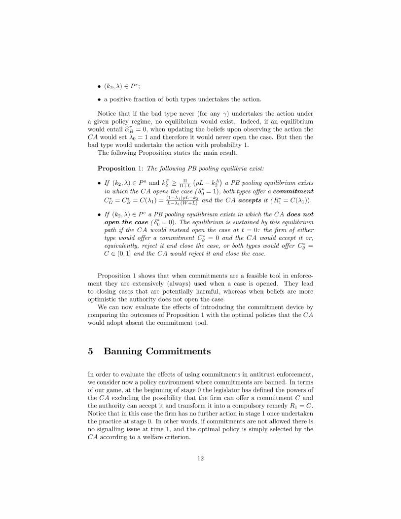
Proposition 1: The following PB pooling equilibria exist:

• If (k2, λ) ∈ P a and kF2 ≥ ΠΠ+L

(ρL− kA2

)a PB pooling equilibrium exists

in which the CA opens the case ( δ∗0 = 1), both types offer a commitmentC∗G = C∗B = C(λ1) = (1−λ1)ρL−k2

L−λ1(W+L) and the CA accepts it (R∗1 = C(λ1)).

• If (k2, λ) ∈ P c a PB pooling equilibrium exists in which the CA does notopen the case ( δ∗0 = 0). The equilibrium is sustained by this equilibriumpath if the CA would instead open the case at t = 0: the firm of eithertype would offer a commitment C∗θ = 0 and the CA would accept it or,equivalently, reject it and close the case, or both types would offer C∗θ =C ∈ (0, 1] and the CA would reject it and close the case.

Proposition 1 shows that when commitments are a feasible tool in enforce-ment they are extensively (always) used when a case is opened. They leadto closing cases that are potentially harmful, whereas when beliefs are moreoptimistic the authority does not open the case.We can now evaluate the effects of introducing the commitment device by

comparing the outcomes of Proposition 1 with the optimal policies that the CAwould adopt absent the commitment tool.

5 Banning Commitments

In order to evaluate the effects of using commitments in antitrust enforcement,we consider now a policy environment where commitments are banned. In termsof our game, at the beginning of stage 0 the legislator has defined the powers ofthe CA excluding the possibility that the firm can offer a commitment C andthe authority can accept it and transform it into a compulsory remedy R1 = C.Notice that in this case the firm has no further action in stage 1 once undertakenthe practice at stage 0. In other words, if commitments are not allowed there isno signalling issue at time 1, and the optimal policy is simply selected by theCA according to a welfare criterion.

12

The following Lemma easily establishes the optimal policies.

Lemma 4: Under Assumption 1, if the CA opens the case at stage 0, thenat stage 1 the following holds:

- if λ1 ∈[0, λ(k2)

)the CA proceeds to stage 2.

- If λ1 ∈[λ(k2), 1

]the CA closes the case.

From Lemma 4 it follows that in the space (k2.λ1) the region where theCA closes the case (region c in the previous section) is the same when com-mitments are feasible or banned, and the region (region a) where commitmentsare.accepted when feasible is the same as the region where the CA proceeds tostage 2 when commitments are banned. Moreover, since in the commitment casethe firm offers the minimum commitment C(λ1) that makes the CA indifferentbetween accepting the commitment and proceeding to stage 2, for given λ1 theexpected welfare at stage 1 under the two regimes is the same. Let us defineregion b where the CA proceed to stage 2 when commitments are banned as:

region b:{

(k2, λ)∣∣∣κ2 ∈

[(1− λ)ρL, ρL

)and λ ∈

[0, λ(k2)

)}Moving back to the end of stage 0, we consider the expected profits and

participation rates of the firm of either type in region b. The expected profitsof the firm of the good type in region b are:

EΠbG = Π

(1− kF2

Π

)(8)

whereas the bad type gets

EΠbB = (1− ρ)Π− ρF − kF2 = Π

[1− kF2

Π− ρΠ + F

Π

]. (9)

We can observe that EΠbB > 0 as long as

ρ < ρ ≡ Π− kF2Π + F

.

Then, we have:

αbG = 1− kF2Π

> αbB = αbG − ρΠ + F

Π> 0 if ρ < ρ. (10)

Hence, when the CA updates the beliefs in region b once observed the actionwe get

λb0 = Λ(λ) =λαbG

αbG − (1− λ)ρΠ+FΠ

> λ.

13

)(~2kλ

λ

2k11 =δ

01 =R

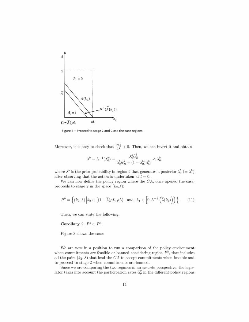
Figure 3 – Proceed to stage 2 and Close the case regions

LρLρλ )1( −

))(~( 21 kλ−Λ

λ

1

Moreover, it is easy to check that ∂λb0

∂λ > 0. Then, we can invert it and obtain

λb = Λ−1(λb0) =λb0α

bB

λb0αbB + (1− λb0)αbG

< λb0.

where λb is the prior probability in region b that generates a posterior λb0 (= λb1)after observing that the action is undertaken at t = 0.We can now define the policy region where the CA, once opened the case,

proceeds to stage 2 in the space (k2,λ):

P b ={

(k2, λ)∣∣∣k2 ∈

[(1− λ)ρL, ρL

)and λ1 ∈

[0,Λ−1

(λ(k2)

))}. (11)

Then, we can state the following:

Corollary 2: P b ⊂ P a.

Figure 3 shows the case:

We are now in a position to run a comparison of the policy environmentwhen commitments are feasible or banned considering region P b, that includesall the pairs (k2, λ) that lead the CA to accept commitments when feasible andto proceed to stage 2 when commitments are banned.Since we are comparing the two regimes in an ex-ante perspective, the legis-

lator takes into account the participation rates αrθ in the different policy regions

14

and for the two types, since at the beginning of time 0 the expected welfare isaffected by the fraction of firms of either type that undertake the action as wellas by the probability of either type. To this purpose let us define

EW r(λ) = λαrGW − (1− λ)αrBL. (12)

This way we can measure the ex-ante effect of the different policy regimes interms of deterrence, that is how they affect welfare through their impact on thedecision of the firms to undertake the action. Then, we can prove the following:

Lemma 5: EW b > EW a.

The intuition can be explained as follows. Moving from an environmentwhere commitments are allowed to one where they are banned, the participationrate of the good type falls, since αbG < αaG. However, this potentially adverseeffect of deterrence is more than counterbalanced by the higher contraction inthe participation rate of the bad type once commitments are unfeasible andthe CA proceeds to stage 2. Hence, overall the ex-ante impact of banningcommitments on deterrence is welfare improving.Deterrence is not the only effect that affects welfare through the participa-

tion rate, since we have also to consider the enforcement effect: how the policiesimplemented affect the final outcome through the firm’s behavior (offering com-mitments when feasible) and the evidence collected in the enforcement phase.Let us define as EW r the expected welfare in the policy region r at the begin-ning of the game. Then, in case commitments are (feasible and) accepted wehave:

EW a(λ) = λαaGW (1− C(λ))− (1− λ)αaB (1− C(λ))L

= (1− C(λ))EW a = (1− C(λ))2EW (λ), (13)

where EW (λ) = λW − (1 − λ)L, since αaθ = 1 − C(λ). The deterrence effectworks through EW a and the enforcement effect is given by 1−C(λ). Since it ispeculiar of the commitment outcome to curtail the welfare effect of the practicein the same way for the good and bad type, the enforcement effect implies atype I error, that is, the practice is reduced when welfare enhancing.Turning to the environment where commitments are banned, we obtain:

EW b(λ) = λαbGW − (1− λ)αbB(1− ρ)L− k2 = EW b + (1− λ)αbBρL− k2 (14)

The enforcement effect when the authority proceeds to stage 2 works throughblocking the practice when the CA obtains hard evidence that it is anticompet-itive. Since ρ < 1, then, type II errors occur, i.e. the practice is not alwaysblocked when anticompetitive.We can now compare the welfare outcomes when commitments are banned

or feasible, in the region P b where the two policy options would be chosenaccording to the tools available. The overall effect of banning commitments iscomplex: although deterrence is more effective when commitments are banned,

15

since ex-post profits and participation of the bad type are reduced more thanthose of the good type, the enforcement effects of the two policy regimes lead toa second best world where type I and type II errors are involved. Commitments,as already argued, apply in the same way to the good and the bad type, andtherefore bring in over-deterrence and type I errors. Conversely, proceeding tostage 2 blocks an anticompetitive practice only when hard evidence is collected,introducing type II errors. Intuitively, weakening a welfare enhancing practice(type I error) is a more serious concern when the practice itself is more likelyto improve welfare, that is when λ is higher. Then, within the region P b wherewe are comparing the policy environments with and without commitments, wewould expect that when λ is relatively high, the commitment regime is lessdesirable, and banning them may improve the policy outcome. When, instead,λ and ρ are low, such that the practice is likely to be anticompetitive butproceeding to stage 2 hardly allows to collect hard evidence and to block thepractice, commitments might become more attractive, saving on type II errors.In the comparison of the commitment and no commitment policy environ-

ments we take a pair (k2, λ) ∈ P b and evaluate the expected welfare in the tworegimes. When commitments are available, the chosen prior λ leads to the sameposterior in stage 0 and 1, i.e. λ = λa0 = λa1 , since deterrence reduces in thesame way the participation rate of the two types, without affecting updatingand posterior beliefs. When instead commitments are banned, the chosen priorλ induces a posterior Λ(λ) = λb0 = λb1 > λ, since deterrence reduces differentlythe participation rate of the two types, affecting positively the posterior beliefs.Hence, the correct comparison of the two regimes for a given pair (k2, λ) ∈ P bis between EW a(λ) and EW b(Λ(λ)) where Λ(λ) = λb0 > λ.

We first establish a preliminary result that is useful to assess the comparison.

Lemma 6: If ρ ∈(

0, 12λ

)the expected welfare when commitments are (fea-

sible and) accepted, EW a(λ), is increasing and concave in λ.

In the following Proposition we state which policy regime is preferable inregion P b.

Proposition 2: Consider the pairs (k2, λ) ∈ P b.For given parameter vectorψ = (ρ, L,W,Π, F, k2) and ρ ∈

(0, 1

2λ

), two cases may arise:

i) If EW a(0) > EW b(0) there exists a λab ∈(

0,Λ−1(λ(k2))such that EW a(λ) ≥

EW b(λ) for λ ∈[0, λab

]and EW a(λ) < EW b(λ) for λ ∈

(λab,Λ−1(λ(k2)

]ii) If EW a(0) < EW b(0) there exists an interval, possibly empty,

[λab, λ

ab],

with 0 ≤ λab ≤ λab

< λ(k2) such that EW a(λ) ≥ EW b(λ) for λ ∈[λab, λ

ab]and EW a(λ) < EW b(λ) for λ /∈

[λab, λ

ab].

16

Proposition 2 establishes that when commitments are a feasible tool, theCA accepts them without concluding the case with a final decision at the end ofstage 2, although for a non empty set of values of (k2, λ) ∈ P b this latter optionwould be preferable in an ex-ante perspective that takes into account not onlythe enforcement stage but also the deterrence effect. Since the CA decides oncommitments at stage 1, when the participation rates are already determinedby the initial decision of the firms of either type to undertake the action, itaccepts the commitment as long as the expected welfare at stage 1 is improved.Indeed, it is the inability of the CA to commit to proceed to stage 2 rejecting thecommitments offered by the firm that moves the authority to accept the firm’soffer too often. When commitments are banned, the CA cannot accept anyoffer by the firm. As a consequence, in this region welfare is improved throughdeterrence. In a nutshell, it is the lack of commitments on the enforcementpolicy that makes the CA biased towards accepting the commitments offeredby the firm.Conversely, when commitments are banned, there may be a non empty region

where giving the firms the possibility to offer commitments and the CA thepower to accept them would improve welfare. This case would arise if the beliefsare pessimistic but the ability of the CA to collect hard evidence and terminatethe practice is very poor. In this latter case, then, a less discriminating butmore effective tool as commitments would allow to limit the welfare losses ofthe practice.

6 Conclusions

7 Appendix

Proof of Lemma 1:. Suppose a PB separating equilibrium C∗G 6= C∗B exists.Then, in equilibrium type θ selects a commitment C∗θ and the CA updates itsbeliefs accordingly upon observing C∗θ : λ1(C∗G) = 1 and λ1(C∗B) = 0.If C∗G > 0, the authority rejects the commitment and closes the case, whereas

when C∗G = 0 the CA is indifferent between rejecting the commitment andclosing the case or accepting the commitment. In all cases the good type obtainsΠG = Π.

When observing C∗B the CA updates its beliefs: λ1(C∗B) = 0. In this caseEW1(R1 = 0) = −L, EW1(R1 = C∗B) = −(1 − C∗B)L and EW1(δ1 = 1) =−(1 − ρ)L − k2. Then, if k2 < ρL, EW1(R1 = 0) < EW1(δ1 = 1) and the CAnever closes the case being certain to face a bad type. Comparing the other twooptions of accepting the commitment or proceeding to time 2, after rearrangingwe conclude that ,if k2 ≤ (ρ−C∗B)L, the CA moves on to a full investigation andaccepts the commitments otherwise. In the former case the bad type optains aprofit ΠB = (1− ρ)Π− ρF while in the latter it gets ΠB = (1− C∗B)Π.Let us check if a deviation is convenient. Type G has no incentive to deviate

since it is getting Π. Consider type B. If it deviates to C∗G it gets Π since the

17

CA cannot detect the deviation. This profit is higher than those if, along theequilibrium path, the CA goes to stage 2 or accepts the commitment. Hence,type B deviates.Then, no separating equilibrium exists.

Proof of Lemma 2:. Consider first the interval λ1 ∈[0, λ(k2)

), where

0 > EW1(δ1 = 1) > EW1(R1 = 0), i.e. carrying on to stage 2 welfare dominatesthe option of closing the case, although both give a negative expected welfare. Ifthe CA decides to proceed to stage 2, the good type expected profits areΠG(δ1 =1) = Π − kF2 whereas the bad type gains ΠB(δ1 = 1) = (1 − ρ)Π − ρF − kF2 .The firm, alternatively, can offer a commitment C yielding, if accepted, Πθ =(1−C)Π. The minimum commitment that makes the CA weakly preferring toaccept it rather than moving to stage 2 is C(λ1) = (1−λ1)ρL−k2

L−λ1(W+L) . Then, if bothfirms offer C∗θ = C(λ1), the CA accepts it.In order to establish if this is a pooling equilibrium we need to check for

deviations. Remind that under passive beliefs any deviation from C(λ1) wouldnot trigger any update in λ1. The CA would accept any commitment higherthan C(λ1) since EW1 < 0 in the interval considered, but this deviation wouldbe unprofitable for the firm of either type. Consider then downward deviations,that lead the CA to reject the commitment and move to stage 2. Since itis the good type that may potentially gain more from moving to stage 2, i.e.ΠG(δ1 = 1) > ΠB(δ1 = 1), the good type prefers to offer the commitment C(λ1)

if Π−kF2 ≤ (1−C(λ1))Π or, equivalently, if kF2 ≥ Π(1−λ1)ρL−kA2L+Π−λ1(W+L) . Since C(λ1)

is decreasing in λ1, the condition kF2 ≥ ΠΠ+L

(ρL− kA2

)is suffi cient to establish

that, for any λ1 ∈[0, λ(k2)

), the good type does not deviate by offring a lower

commitment and making the CA moving to stage 2.

Let us turn now to the case λ1 ∈[λ(k2), λ

). In this interval we have 0 >

EW1(R1 = 0) ≥ EW1(δ1 = 1). If the firms offer a commitment C∗ = 0 theCA is indifferent between accepting it or rejecting and closing the case. Thetwo alternatives, however, are payoff equivalent for the firm and the CA. Noupwards deviation in the commitment is profitable, since the CA would acceptit, being EW1 < 0, and the profits would be lower. No pooling equilibriumwith positive commitment exists, since either type would have an incentive todeviate and offer C = 0.Finally, consider the interval λ1 ∈

[λ, 1]. Here closing the case still welfare

dominates going to stage 2. Moreover, since EW1 ≥ 0, with strict inequality forλ1 > λ, the CA would never accept a positive commitment C > 0, preferringto close the case. In the first equilibrium outcome the firm of either type offersC∗ = 0 the CA is indifferent between accepting it or rejecting and closing thecase. No upward deviation C > 0 would be accepted. Alternatively, in thesecond equilibrium outcome the firm of either type offers C∗ ∈ (0, 1] and theCA rejects it and closes the case. A downward deviation to C = 0 would yieldthe same profits.

18

Proof of Lemma 3:. Let us consider the expected profits of the good and thebad types in the two regions, taking into account that αrθ =

EΠrθΠ . If stage 1 is

reached, then the firm of either type offers in the pooling equilibrium in regiona the commitment C(λ1). Moreover, it anticipates that at t = 1 no updatingin beliefs will occur, and therefore λ0 = λ1. Finally the firm of either typewill obtain the same expected profits, and therefore αaG = αaB . Consequently,the firm anticipates that no updating will occur at stage 0, and λ0 = λ. Theexpected profits at the beginning of stage 0, therefore, are

EΠaθ = (1− C(λ))Π.

Consider next the expected profits if the case will not be opened, since it wouldbe eventually closed at stage 1. In this case

EΠcθ = Π.

Proof of Proposition 1:. In region P a when the case is opened then the firmof either type offers a commitment that is accepted by the CA, according to thestatements of Lemma 2. The participation rate of the good and bad type areidentified in Lemma 3 and lead to the same rate of adoption αaG = αaB = 1−C(λ)

that is positive for any λ ∈[0, λ(k2)

). Hence, λ0 = λ when the CA observes

that the action has been undertaken. Since the firm of either type offers thesame level of commitment, no updating occurs also at stage 1 and λ1 = λ0 = λ.Then„according to the definition of P a, all the equilibrium conditions are metand the equilibrium exists.Finally, in region c the CA does not open the case at t = 0. Notice that

in this case αcG = αcB = 1 and, upon observing the action, λ0 = λ. If the CAwould instead open the case, Lemma 3 describes the equilibrium choices. Then,according to the definition of P b, all the equilibrium conditions are met and theequilibrium exists.

Prof of Lemma 4:. From the definition of λ(k2), EW1(δ1 = 1) > EW1(R1 =

0) for λ1 ∈[0, λ(k2)

)and vice versa. Then, the optimal policies described in

the statement immediately follow.

Proof of Lemma 5:. When commitments are feasible and accepted (regiona), αaθ = 1−C(λ). Then EW a = (1− C(λ))EW (λ), where EW (λ) = λW−(1−λ)L. When instead commitments are banned (region b), we have αbG = 1− kF2

Π

and αbB = αbG − ρΠ+FΠ . Hence, EW b = αbGEW (λ) + (1 − λ)ρLΠ+F

Π . Then,

EW b > EW a can be rewritten as:

(1− λ)ρLΠ + F

Π> EW (λ)

(kF2Π− C(λ)

)

19

that holds since the LHS term is positive while the RHS is negative, beingEW (λ) < 0 for λ < λ, as it is in regions P a and P b, while kF2 > C(λ)Π toensure that a PBE pooling equilibrium exists in P a.

Proof of Proposition 2:. We first establish that for ρ ∈(

0, 12λ

)the expected

welfare when commitments are accepted, EW a(λ) = (1− C(λ))2EW (λ), is

increasing in λ. Notice that when λ increases, the commitment becomes lessgenerous and a larger fraction of the (negative) expected welfare is realized. Atthe same time, more optimistic beliefs improve the expected welfare. Indeed:

∂EW a

∂λ= (1− C(λ))

[(1− 2λ+ λ)ρL− k2 − EW1

−EW1

](W + L) .

Let us denote A = (1 − 2λ + λ)ρL − k2 − EW1. Then, sign∂EWa

∂λ = signA.Notice that ∂A∂λ = −(W + (1− ρ)L < 0. Hence, the stricter conditions to obtainA > 0 are at λ = λ(k2) = 1− k2

ρL . Then,

A(λ(k2), k2

)= 2

[(1− λ)ρL− k2

]−W +

k2

ρL(W + L)

for k2 ∈[(1− λ)ρL, ρL

). Then, we have A

(λ((1− λ)ρL), (1− λ)ρL

)= 0,

∂A(λ(k2),k2)∂k2

= 1ρλ− 2 > 0 for ρ ∈

(0, 1

2λ

), we conclude that A

(λ(k2), k2

)≥ 0

for k2 ∈[(1− λ)ρL, ρL

)with strict inequality for k2 > (1 − λ)ρL. Then, for

ρ ∈(

0, 12λ

)we have A (λ(k2), k2) ≥ 0 and ∂EWa

∂λ ≥ 0 for k2 ∈[(1− λ)ρL, ρL

)with strict inequality for k2 > (1− λ)ρL. Moreover,

∂2EW a

∂λ2 = −22[(1− λ)ρL− k2

]2(−EW )3

< 0.

Hence, EW a(λ) is increasing and concave in λ.The expeced welfare in region b, instead, is

EW b(λ) = λαbGW − (1− λ)αbB(1− ρ)L− k2

and is therefore increasing and linear in λ.Consider then EW b and EW a at the upper bound of region P b, i.e. for

k2 and λ = Λ−1(λ(k2). Then, if the CA proceeds to stage 2 since no com-mitment is available, the deterrence effect improves the posterior belief andλb0 = Λ(Λ−1(λ)) = λ. If, instead, commitments are available, since the samepair belongs also to region P a, the CA accepts the commitment. In this case thepolicy undertaken does not affect the posterior, i.e. λa0 = Λ−1(λ) < λ. Hence, wehave to compare EW b(λ) and EW a(Λ−1(λ)). Since Λ−1(λ) < λ and EW a(λ)

is increasing in λ, as previously established, then EW a(Λ−1(λ)) < EW a(λ).Notice that since C(λ) = 0, then

EW a(λ) = λW − (1− λ)L = EW (λ).

20

The expected welfare when commitments are banned, instead, is

EW b(λ) = λαbGW − (1− λ)αbB(1− ρ)L− k2

that, after rearranging, can be written as

EW b(λ) = αbGEW (λ) + k2

[αbB +

F

Π

].

Notice that, since EW (λ) < 0, we have:

EW b(λ) > EW a(λ) > EW a(Λ−1(λ)).

Hence, at the upper bound of region P b banning commitment is welfare improv-ing. Since both functions are continuous in λ the above inequalities hold truealso in aneighborhood of the upper boundary of region P b.

Consider next the two expressions at the lower bound λ = 0, that impliesλc0 = Λ(0) = 0. Since C(0) = ρL−k2

L , we have

EW a(0) = − [(1− ρ)L+ k2]2

L

andEW b(0) = −

[(1− ρ)αbBL+ k2

].

Then, if at the lower bound of P b, λ = 0, we have EW a(0) > EW b(0), since theformer is increasing and convex whereas the latter is increasing and linear in λ,and EW b(λ) > EW a(Λ−1(λ)) at the upper bound of P cb, there exists a singleλ, for given parameters ψ, such that EW c(λ) = EW a(Λ−1(λ)), i.e EW c(λ) andEW a(λ) intersect only once at λ. Then, accepting the commitment is welfareincreasing for λ ≤ λ and banning commitments is optimal for λ ≥ λ. SinceαbB ∈ (0, 1), we can write the condition EW a(0) > EW b(0) as

[(1− ρ)L+ k2]2

L<[(1− ρ)αbBL+ k2

].

Notice that for parameter values such that αbB ∼= 0, the above inequality holds.Indeed, letting x = (1−ρ)L+k2 > 0, the above inequality can be approximatelywritten as x2

L − x < 0 or, equivalently, x < L. Since k2 ∈((1− λ)ρL, ρL

),

by substituting in x we can observe that the inequality always holds. Hence,EW a(0) > EW b(0). In this case, due to continuity, for λ ∈ [0, λ(ψ)] the policyoutcomes when commitment is available dominate while banning commitments

is socially beneficial for λ ∈[λ(ψ),Λ−1

(λ(k2)

)]. When, instead, the above

inequality never holds, then introducing commitments is always welfare detri-mental.Proof of Lemma 6:. Consider EW a(λ) = (1 − C(λ))2EW (λ). Whenλ increases the commitment becomes less generous and a larger fraction of the

21

(negative) expected welfare is realized. At the same time, more optimistic beliefsimprove the expected welfare. Indeed:

∂EW a

∂λ= (1− C(λ))

[(1− 2λ+ λ)ρL− k2 − EW1

−EW1

](W + L).

Let us denote A = (1 − 2λ + λ)ρL − k2 − EW1. Then, sign∂EWa

∂λ = signA.Notice that ∂A∂λ = −(W + (1− ρ)L) < 0. Hence, the stricter condition to obtainA > 0 is at λ = λ(k2) = 1− k2

ρL . Then,

A(λ(k2), k2) = 2[(1− λ)ρL− k2

]−W +

k2

ρL(W + L)

for k2 ∈[(1− λ)ρL, ρL

]. Hence, we haveA(λ(k2), k2) = 0 for k2 = (1−λ)ρL and

∂A(λ(k2),k2)∂k2

= 1ρλ−2 > 0 for ρ ∈

(0, 1

2λ

). Then, we conclude that A(λ(k2), k2) ≥

0 for k2 ∈[(1− λ)ρL, ρL

]. Therefore, for ρ ∈

(0, 1

2λ

)we have A(λ, k2) ≥ 0 and

∂EWa

∂λ ≥ 0 for k2 ∈[(1− λ)ρL, ρL

], with strict inequality for k2 > (1− λ)ρL.

Turning to the second derivative,

∂2EW a

∂λ2 = −∂C∂λ

A

−EW1+ [1− C(λ)]

[W + (1− ρ)L]EW1 +A(W + L)

(−EW1)2

that, after rearranging, becomes

∂2EW a

∂λ2 = −C(λ)A(W + L)

(−EW1)2D(λ, k2)

where D(λ, k2) = A + (1 − C(λ)EW1. Then, since C(λ) < 0, sign∂2EWa

∂λ2=

signD(λ, k2). Evaluating D).) we get:

D(λ(k2), k2) = (1− λ)ρL− k2 ≤ 0

D(0, k2) = 2[(1− λ)ρL− k2

]≤ 0

for any k2 ∈[(1− λ)ρL, ρL

], with strict inequality for k2 > (1− λ)ρL. Hence,

∂2EWa

∂λ2≤ 0 in P b with strict inequality for k2 > (1− λ)ρL.

Proof of Proposition 2:. We compare in region P b the expecged welfarewhen commitments, being feasible, are indeed chosen as the preferred policyoption,

EW a(λ) = (1− C(λ))2EW (λ)

with the expected welfare when, banning commitments, the CA runs a fullinvestigation:

EW b(λ) = EW b + (1− λ)αbBρL− k2.

In Lemma 6 we have established that EW a(λ) is increasing and concave in λprovided ρ < 1

2λ. From inspection, instead, EW b(λ) is increeasing and linear in

22

λ. Consider then EW a(λ) and EW b(λ) at the upper boundary of region P b, fork2 ∈

[(1− λ)ρL, ρL

]and λ = Λ−1(λ(k2)). When commitments are banned and

the CA proceeds to full investigation, λb0 = Λ(

Λ−1(λ(k2)))

= λ(k2). If, instead,

commitments are available, since P b ⊂ P a, the CA accepts the commitmentswhen (k2, λ) ∈ P b. In this case, λa0 = Λ−1(λ(k2)) < λ(k2). Hence, we have to

compare EW b(λ(k2)) and EW a(

Λ−1(λ(k2))). Since Λ−1(λ(k2)) < λ(k2) and

EW a(λ) is increasing in λ, then EW a(

Λ−1(λ(k2)))< EW a

(λ(k2)

). Notice

that, since C(λ(k2)

)= 0, then

EW a(λ(k2)

)= λ(k2)W − (1− λ(k2))L = EW (λ(k2)).

The expected welfare when commitments are banned computed at λ(k2), in-stead, is

EW b(λ(k2)

)= λ(k2)αbGW − (1− λ)αbB(1− ρ)L− k2 =

= αbGEW (λ(k2)) + k2

(αbB +

F

Π

).

Then, since EW (λ(k2)) < 0 we have:

EW b(λ(k2)

)> EW a

(λ(k2)

)> EW a

(Λ−1(λ(k2))

).

We conclude that at the upper boundary of region P b banning commitments iswelfare improving.

Since EW b(λ(k2)

)> EW a

(Λ−1(λ(k2))

)and EW b (λ)EW a is increasing

and linear in λ whereas EW a (λ) is increasing and concave in λ, it may be that

the two curves intersect once, two times or never for λ ∈[0,Λ−1(λ(k2))

]. To

sort these cases let us consider the two expressions at the lower bound λ = 0,that implies λb0 = Λ(0) = 0. SInce C(0) = ρL−k2

L , we have:

EW a(0) = − [(1− ρ)L+ k2]2

Land EW b(0) = −

[(1− ρ)αbBL+ k2

].

If EW a(0) > EW b(0), the two curves intersect once at λab since EW b(λ(k2)

)>

EW a(

Λ−1(λ(k2))). When, instead, EW a(0) < EW b(0) it may happen that

EW a(λ) > EW b(λ) in a compact set[λab, λ

ab]or that EW a(λ) < EW b(λ)

always holds true.

23