Unions and the Labor Market for Managers

John DiNardoUniversity of California – Irvine,

University of California – Berkeleyand

NBERKevin F. Hallock

University of Illinois at Urbana–ChampaignJorn-Steffen Pischke ∗

Centre for Economic PerformanceLondon School of Economics and NBER

August 2000

Keywords: Executives, managers, unions, wage structure, CEOs

JEL Classification: J31, J44, J51

∗ DiNardo: Dept. of Economics, University of California, Irvine, CA on leave at Department ofEconomics, University of California, Berkeley, CA, 94720, jdinardo@uci.edu. Hallock: Dept. of Economicsand Institute of Labor and Industrial Relations, University of Illinois at Urbana–Champaign, Champaign,IL 61820, hallock@uiuc.edu. Pischke: Centre for Economic Performance, London School of EconomicsLondon, England, WC2A 2AE, s.pischke@lse.ac.uk. We thank John Abowd, Danny Blanchflower, BarryHirsch, Kevin Murphy, Joe Tracy and Michael Wallerstein for data, Ben Gordon for excellent researchassistance, and Daron Acemoglu, Danny Blanchflower, Donald Deere, Sue Dynarski, Pete Feuille, WallyHendricks, Barry Hirsch, David Lipsky, David Lewin, and Sendhil Mullainathan. We are grateful to theAmerican Compensation Association for financial support. The views expressed are solely the authors anddo not reflect the views or opinions of the American Compensation Association.

1

Unions and the Labor Market for Managers

Abstract

We examine the relationship between the employment and compensation of managersand CEOs and the presence of a unionized workforce. We develop a simple effciencywage model, with a tradeoff between higher wages for workers and more monitoring,which requires more managers. The model also assumes rent sharing between work-ers, managers and the owners of the firm. Unions, by redistributing rents towardsthe workers, lead to lower employment and lower pay for managers. Using a varietyof data sets, we examine the implications of the model for the relationship betweenthe employment and wages of managers and unionization. We find several resultsgenerally consistent with our model. (1) Both a higher fraction of unionization in anindustry and region and a higher union wage differential are associated with fewermanagers. (2) Managers wages are about 5 to 7 percent lower in unionized firms.(3) For CEOs the effects are larger: a 10 percent increase in unionization reduces thepay of CEOs by 2.5 percent or more.

Keywords: Executives, managers, unions, wage structure, CEOs

JEL Classification: J31, J44, J51

1 Introduction

Union representation limits management’s discretion to set the wages of covered workers

and management is required to bargain with the workers’ union. The effect of this process

on the wages of union workers is clear: unions raise the wages of their members. Abowd

(1989) finds that collective bargains are “efficient” (in the sense of maximizing the sum of

shareholders’ and union members’ wealth). Given the evidence that profits are lower in

unionized firms (Clark 1984) this suggests that unions redistribute rents from the owners

of firms to the workers. If this is the case, it is likely that other constituents in the firm

also gain or lose from the presence of unions. In this paper, we look directly at the impact

unionization has on employment and compensation of managers.

Bargaining and rent redistribution are likely to be the key mechanisms through which

unions impact the employment and pay of managers. At bargaining time and more visibly

during periods of industrial disputes, workers often voice concern over the pay and com-

pensation of managers and executives. Anecdotal evidence suggests that when workers are

organized, executives or directors feel more pressure to limit the pay of managers. DeAn-

gelo and DeAngelo (1991), for example, find that corporate executives and other white

collar workers accepted major pay cuts in years where steel firms sought to obtain pay

concessions from blue collar workers in union negotiations.

A large literature in corporate finance tries to analyze the incentives of managers to

create and appropriate rents (Jensen and Meckling 1976). This literature has primarily

focused on the role of large shareholders, boards of directors, and takeover threats in

disciplining management. There is little consideration of how other stakeholders in the

firm, like workers, might influence the way the firm is run, and how rents are created and

distributed. But in the process of redistributing rents from shareholders and management

1

to members, unions affect the behavior of firms in many ways. While there is mixed

evidence that unions seem to lower investment and the growth of firms (Blanchflower,

Millward and Oswald 1991, Bronars, Deere and Tracy 1994, Machin and Wadhwani 1991)

there is some evidence that they raise productivity in some circumstances (Allen 1984,

Bronars et al. 1994). This combination of effects may appear counterintuitive at first

blush. One explanation has been suggested by Freeman and Medoff (1984) – these effects

might be explained by the role of unions as a voice for workers. Another channel, and the

possibility we investigate here, is that that unions may directly affect the way firms are

managed.

We view the role of managers primarily as supervising and monitoring workers. Because

monitoring is imperfect, workers will be paid an efficiency wage. Through bargaining,

however, unions redistribute rents towards workers, setting a wage above the level that

the firm would have chosen. This makes union jobs more attractive relative to outside

alternatives. This, in turn, reduces the need for monitoring, and therefore the firm’s

need to employ managers. Since the monitoring of workers requires real resources, this

process will raise productivity and (static) social welfare, even though unions may impede

the investment and growth of unionized firms. This effect has first been discussed by

Acemoglu and Newman (1997). The model for the managerial labor market which we

present in section 2 builds on their work.

To the best of our knowledge, there is no previous empirical work investigating the

link between unionization and executive pay and employment. Our paper tries to fill this

gap. To this end we have assembled a variety of different datasets. We begin our empirical

investigation in section 3, by analyzing a panel of grouped data by region and industry,

which we constructed from the 1983 to 1993 Current Population Surveys for the U.S. These

data allow us to examine both the employment and wage effects of unions. In addition, we

attempt to tackle the problem that unionization of industries is not chosen randomly, but

is likely driven by the presence of rents in a sector. These rents will also be reflected in

2

wages, therefore creating a spurious positive correlation between wages of managers and

unionization. We use industry wage differentials for non-union workers as a proxy for the

rents present in a sector.

In section 4, we use several sources of data on the compensation of U.S. CEOs and

unionization at the level of firms. Since the pay of the top executive of publicly held

companies has to be disclosed annually, we focus on CEO compensation for the firm level

analysis, as does most of the literature on executive pay. Hirsch (1991) and Bronars et

al. (1994) have assembled data on the unionization of particular U.S. firms. We use their

data together with the pay data for CEOs to investigate the link between unionization and

executive pay.

Finally, in section 5 we investigate cross-national data on unionization and the propor-

tion managers in the labor force and CEO pay, both of which differ substantially across

countries. We have assembled data on the fraction of managers employed in a variety of

countries, which we use in conjunction with a dataset created by Abowd and Bognanno

(1995) on CEO compensation. Using all of these different data sources we find the con-

sistent result that unions tend to lower both the employment and the wages of managers

and executives. We also find that the presence of rents tends to distort this relationship.

Section 6 discusses the results and concludes.

Apart from the theoretical analysis by Acemoglu and Newman (1997), we are not aware

that the link between unionization and the managerial labor market has been investigated

formally before. Our work is related to three different literatures. First, our paper is

linked to the literature on the impact of unions on economic outcomes. Freeman and

Medoff (1984) briefly discuss the impact of unions on white collar workers within the same

firm (who seem to gain from unionization), but they do not discuss the most highly paid

workers: managers and top executives.

Second, our work contributes to the growing literature on CEO compensation. The

compensation of top executives varies widely across firms. Although the focus of much

3

of the literature has been on the role of firm performance in CEO compensation (Gregg,

Machin and Szymanski 1993, Jensen and Murphy 1990), it appears to account for little

of the variation in the level of CEO pay across firms.1 A related literature has attempted

to explain cross-sectional differences in CEO pay. Joskow, Rose and Shepard (1993), for

example, ask whether political pressures may limit the level of CEO pay. They find that

CEO compensation is lower in regulated industries and that pay is less sensitive to firm

performance in these industries. Joskow, Rose and Wolfram (1996) link CEO pay in

the electric utility industry even more directly to specific regulatory practices. Akin to

regulation, which gives a particular stakeholder group (customers) more voice, unions may

be able to affect the pay of CEOs for their own benefit.

Third, there is a link between our investigation and the recent literature on changes in

wage inequality. Freeman (1993), Card (1992), and DiNardo, Fortin and Lemieux (1996)

have found that the decline in unionization can explain roughly 30 percent of the recent

increase in wage inequality in the U.S., while Bell and Pitt (1998) put this number at about

25 percent for the U.K. Moreover, DiNardo and Lemieux (1997) also find an association

between the change in unionization and changes in wage inequality comparing the U.S.

and Canada. These studies, however, focus only on the unions’ wage impacts on covered

workers. Since unionized workers typically occupy the lower and middle part of the wage

distribution, these papers do not attempt to account for changes in wage inequality that

have taken place among non-unionized workers in the top of the wage distribution. If the

presence of unions has an impact on the pay of the highly paid as well, however, the decline

of unionization in countries like the U.S. and the U.K. might explain an even larger part

of the spreading in the wage distributions. This effect would be much more difficult to

uncover with these within country accounting exercises. Cross country regressions, as in

1This is abstracting from the variability introduced by revaluations of stock and option grants as stressedby Hall and Liebman (1998). A survey of the literature can be found in Conyon, Gregg and Machin (1995)and Murphy (1999).

4

Freeman (1996), on the other hand, should estimate the full effect of unions on the wage

distribution.

2 A Simple Model

In this section we present a stylized model of the labor market for managers in an economy

with unions. The role of managers is to monitor workers. The monitoring technology in

the unionized sector is imperfect, so that, in the absence of supervision, workers would not

exert enough effort. However, the firm can trade off paying higher wages with hiring more

managers, along the lines of the model in Acemoglu and Newman (1997). This implies

that unions, by raising the wages of their members, and therefore diminishing the need for

supervision, will lower the demand for managers.

Unions also interact with the labor market for managers in a second way. Firms in

the unionized sector generate rents which are shared with the employees. It is these rents

which attract unions to the sector in the first place. This means that unions are more

likely to exist in sectors which pay higher wages, not just to workers but also to managers.

On the other hand, unions also redistribute rents from managers to workers. The model

therefore does not predict unambiguously whether unions are associated with higher or

lower wages for managers.

The model economy consists of two sectors, a unionized sector and a competitive sector.

We will take conditions in the competitive sector as given, and concentrate on the wage

and employment determination for managers in the unionized sector. Technology in both

sectors requires workers to exert effort. However, the sectors differ in that monitoring

is perfect in the competitive sector, so that firms can easily enforce no shirking. The

monitoring technology in the unionized sector is imperfect. Workers who shirk will be

caught with probability q < 1. Shirkers who are detected lose their job in the unionized

sector, but they find employment in the competitive sector at wage w∗L during the same

5

period. Effort requires a utility cost e, so that the no shirking condition in the unionized

sector is given by

wL − e ≥ (1− q)wL + q(w∗L − e).

Workers who supply effort receive a wage wL, but have to pay effort cost e. Workers who

shirk will not be caught with probability 1 − q, in which case they do not have to pay

the effort cost. With probability q they are caught shirking, in which case they are laid

off and have to work in the competitive sector at wage w∗L. Recall that they will have to

put forth effort in the competitive sector as well and shirking is not possible in that sector

because of perfect monitoring.2 Rearranging the expression above yields

wL ≥ w∗L +1− qq

e. (1)

Firms in the unionized sector can choose the monitoring intensity, given by q. In

particular, we assume that q = q(m) is a function of the number of managers the firm

hires per worker, given by m. q(m) is an increasing and concave function. The firm takes

wages for managers and workers as given, and maximizes profits

maxm,L

π = pf(L)− wMmL− wLL (2)

subject to the no shirking constraint in (1), where L is the number of workers, mL is the

number of managers hired, and p is the price of the good. Profit maximization implies

that (1) always holds as an equality in equlibrium. This is because the firm can always

reduce the number of mangers hired for a given worker wage until the constraint is no

longer slack, thus reducing costs without changing worker incentives (see Acemoglu and

2We assume that w∗L − e exceeds the workers’ reservation utility, so that they will always want toparticipate in the competitive sector of the economy.

6

Newman (1997)).

Wages for workers and managers in the unionized sector are determined by bargaining

over rents. Rents R generated by a particular firm are

R = pf(L)− w∗MmL− w∗LL

where w∗i denotes the competitive wage for group i. The firm cares about profits, while

workers and managers care about the surplus they receive compared to working elsewhere

SM = (wM − w∗M)mL

SL = (wL − w∗L)L

where Si is the surplus. Three-way Nash bargaining maximizes

SaMSbLπ

1−a−b

and a and b are the bargaining parameters of managers and workers, respectively. We

assume that these bargaining parameters depend on the degree of unionization, with

a′(U) < 0 and b′(U) > 0. This leads to the wage rules3

wM = w∗M + a(U)R

mL(3)

wL = w∗L + b(U)R

L.

Employment and wages for managers in the unionized sector are now easy to determine.

(1) written as an equality determines employment for managers. Define Q(m) ≡ (1 −3In principle, firms may want to set a higher wage for workers than the bargained wage if the bargained

wage was below the profit maximizing efficiency wage. In practice, this will not occur, because unionswill realize this and push the wage for workers up even further. Therefore, this constraint is implicitlytaken into account in the bargaining parameters a and b.

7

q(m))/q(m). Q is a strictly decreasing function. It can therefore be inverted to yield

m = Q−1

(wL − w∗L

e

)(4)

= Q−1

(b(U)R/L

e

)

using the wage equation (3) for workers. Higher rents and more unionization are associ-

ated with fewer managers per worker. This is because rents and unions raise the wage

differential for workers, make shirking less attractive, and therefore reduce the need for

direct monitoring.

Equation (4) also makes clear, that in a unionized firm it is only the union wage

differential wL−w∗L that should matter for the fraction of managers hired. We can control

for the union wage differential at the industry level directly in our empirical estimates.

However, note that the interpretation of equation (4) at the industry level will differ if

there are both union and non-union firms in the industry. The fraction of managers hired

in union firms will generally be lower than in non-union firms. It will also be lower in

unionized firms the higher the union wage differential. This illustrates that the fraction

of managers at the industry level still depends on both the union wage differential and the

unionization rate.

Unions only affect managers in the model because they raise wages for workers. It is

well known, however, that unions also change other aspects of the employment relationship.

One is layoff rules. The fact that it is more difficult to fire union workers may imply that

the layoff probability q is directly a function of the unionization rate, i.e. q(m,U) with

∂q/∂U < 0. Through this channel, unions will make shirking more attractive, because the

penalty of a layoff is less likely. This means that the firm will have to hire more managers, in

order to raise the probability of detection, but also to document worker misbehavior more

carefully, pursue grievances, etc. In this expanded version of the model, the net effect on

8

managerial employment is ambiguous, since higher wages still deter shirking. Therefore,

which channel is more important is an empirical question. Since we find large negative

effects of unions on managerial employment below, we conclude that the effect of unions

on wages is the more important ingredient of the model.

However, is also possible that rent-sharing alone determines both wages and employ-

ment for managers. In this view, more rents will be used by managers for empire builing.

This implies hiring more subordinates, i.e. lower level managers, thus creating an unnec-

essarily large and bloated organization. In this case, higher rents are associated with more

managers not fewer, as in equation (4). Most of our results do not speak to the distinction

between these two views directly, since we investigate the effect of unionization rather than

rents on the level of employment of managers. However, some of our results in Table II

below are consistent with the rent-sharing view of mangerial employment.

Wages for managers are given by (3), which implies that more unionization leads to

lower wages for managers, because unions are able to redistribute rents from the firm’s

owners and from managers towards workers. However, note that this relationship only

holds for a given level of rents. In order to close the model we need to discuss how

unionization in an industry is determined. The degree of unionization should depend

on the benefits and costs of unionization. Ceteris paribus, unions will tend to organize

industries with higher rents. However, costs of organizing different industries will differ.

For example, manufacturing firms with few large plants may be easier to organize than

service firms with many small establishments. Industries will also differ in how easy it is

to raise wages in the industry, implictly given by the shape of b(U) in our model. This can

be summarized as

U = U(R, state and industry characteristics).

It is clear from this discussion that the wages of managers may be positively associated

9

with the degree of unionization if rents are not adequately controlled for. One way to

control for this problem empirically would be to use state and industry characteristics

to instrument for unionization rates. However, it is difficult to find observables that

are powerful enough to predict unionization rates, especially variation within regions and

industries over time. We therefore concentrate on proxying rents directly. In particular,

we use the industry wage differential for non-union workers as a control. The rationale for

this is the evidence that industry wage differentials are likely due to rent sharing, and that

these rents are shared with all workers, not just union workers (see Katz and Summers

(1989), and Dickens and Katz (1987)).4 One complication with this strategy is that unions

may affect the rents earned by a firm directly. In this case, it would be difficult to interpret

the coeffcient on the unionization variable controlling for rents (see Angrist and Krueger

(1999)). However, since rents are difficult to measure there is no empirical evidence that

workers influence rents directly. In addition, controlling for rents is the best strategy we

have available for estimating the causal effect of unionization on the pay and employment

of managers.

Our discussion of the factors driving unionization in an industry highlights that we are

relying on cost factors to identify the unionization variable. This implies that it should

be more difficult to identify the effects of unionization and rents separately if we try to

control for industry effects directly, thus purging the unionization variable of much of its

identifying variation.

How can we use this model to think about the compensation of CEOs? Clearly, we

can apply the wage equation (3) in a similar way as for lower level managers. On the

other hand, there is one CEO per firm, so there is no natural quantity measure reflecting

the intensity of CEO use. We assume that firms or industries which use managers more

intensively (i.e. have a higher fraction of managers), will need a more skilled CEO. We

4Note that this is not really inconsistent with the model above. Wages in the “competitive” (non-union)sector w∗L may also reflect rents.

10

therefore expect higher pay for CEOs wherever we see more managers employed. Since

unions should depress the employment of managers we expect to be more likely to find a

negative corrrelation between unions and the pay for CEOs as compared to the pay for

lower level managers.

3 Industry Level Results for U.S. Managers

While the theoretical analysis suggests that we examine the concentration of managers in

unionized versus non-unionized firms, data on the fraction of managers are not as readily

available at the firm level. However, the implications of the theory can also be investigated

with data at the industry level. Hence, we follow the strategy of Neumark and Wachter

(1995), and analyze the pay of managers at the level of industry and regional cells, which we

construct from the Current Population Survey (CPS). Neumark and Wachter use industry

level data from the CPS for the period 1973 to 1989 and find that a 10 point higher fraction

of blue collar workers unionized in an industry is associated with 1.8 percent lower wages

for managers and professionals.

We use the 1983 to 1993 Merged Outgoing Rotation Groups from the CPS to construct

cells at the industry/region/year level. Our sample starts in 1983 because this is the first

year where union status is available for the outgoing rotation groups. In order to have cells

of sufficient size, we aggregated two digit industries into 26 broader industries, and states

into 16 regions. A complete list of the industry and state cells used is given in Appendix

1. The key occupation group we are interested in is executives and managers (1980 3-digit

SIC occupation codes 3-22). These are primarily occupations who supervise others. In

principle, workers in this group cannot form unions under NLRB rules. However, the

line between this group of managers and management related occupations and business

specialists like accountants, analysts, inspectors, etc. is often not very clear. We therefore

also present results on this second group (occupation codes 23-37). We refer to the occu-

11

pations in SIC codes 203-889 as workers. This includes all occupations except managerial

and professional occupations. We split the group of workers into those who are covered

by collective bargaining themselves, and non-union workers. Our samples are restricted to

those working five or more hours, who are in the private sector and not self-employed, and

with valid wage and occupation information in the CPS.

Table I provides means of the characteristics of these four groups (managers, man-

agement related occupations, non-union and union workers) for the years 1983 and 1993.

Managers and union workers tend to be older (and have more potential experience) than

the other groups. For each of these groups we report two measures of unionization. The

fraction unionized in the occupation refers to the fraction of observations in this occupa-

tion who respond that they are covered by a union contract. Between 5 and 6 percent

of managers and related occupations in 1983 report that they are covered by collective

bargaining. This is surprising since we do not expect managers to be organized in unions.

This result may be due to measurement error because either the union or the occupation

question are answered or coded incorrectly. However, 5 percent seems a little too high as

compared with typical misclassification rates (Card 1996) so that some of this may reflect

actual unionization of this group. Some managers may be in relatively low level positions,

who do not directly supervise others, and who are therefore not subject to NLRB rules.

When we run standard cross-sectional wage regressions, we find that unionized managers

have roughly 8 percent higher wages than other managers, about half the union wage dif-

ferential typically found for all workers. This also seems to indicate that at least some of

this may reflect actual unionization of the group.

The penultimate row in each panel in Table I reports the fraction of unionized workers

(those who are neither managers, related, or professionals) in the industry/region cells

to which a manager or worker belongs. If all occupations were equally distributed across

these cells, this number would be constant across the different columns (except for sampling

variation) and would reflect the unionization level of workers in the economy. But different

12

occupations tend to be more concentrated in certain industries. For example, there are

more managers in banking and other finance than there are in the construction industry.

Since the unionization rates of workers in these industries differ, and since the reported

means for managers, say, are weighted by the number of managers in a cell, the fraction

of union workers reported for each occupation differs. Thus, the fraction of union workers

refers to the exposure of the occupation to unionized workers in the particular cell. The

most notable, but unsurprising result about this fraction is that union workers tend to

be concentrated in industry/region cells which are more highly unionized. Exposure to

unionized workers has declined for all occupations over time. The last row in each panel

reports the fraction of managers in the industry/region cell to which an occupation belongs.

This fraction differs little by occupation. For each occupation there is about a 1.5 or 2

percentage point increase in the fraction of managers over the sample period.

In order to assess the effect of unions on the pay of managers, we estimate a regression

of the form

lnwsijt = Xsijtβ + γusjt + µj + ηs + δt + εsijt.

wsijt is the wage of individual i in industry j and state s at time t. Xsijt is a set of covariates

which includes years of schooling, potential experience and its square, and dummies for

female, black, whether the individual lives in an SMSA, and part-time status (less than 35

hours a week). usjt is the fraction of workers who are unionized in each state/industry/time

cell. Notice that this variable does not vary at the individual level. In order to implement

the estimation of this model and to obtain standard errors robust to a group structure in

εsijt we first regressed lnwsijt on Xsijt and a full set of industry/state/year interactions. In a

second stage, we regressed the coefficients from these dummy variables on the fraction of

workers unionized in the industry. The second stage regression is weighted by the number

of observations in the cell. The results from the second stage regression are shown in

13

Table III (see below). In order to examine the effect of unions on the employment of

managers, we pooled the observations for all occupations in a state/industry/year cell,

calculated the fraction of managers in the cell, and regressed it on the fraction of unionized

workers.

Table II displays results of the employment regressions in two panels for the dependent

variables, fraction managers and fraction managers and related occupations. In the first

column of the top panel we display estimates from a regression of the fraction of managers

in the cell on the fraction of workers unionized. This and all the following regressions

also control for separate industry, region, and year effects. These effects are necessary to

account for the different employment structures of various industries and regional differ-

ences. The effect of unionization on the employment of managers is strongly negative and

significant. A 10 percentage point increase in the unionization rate leads to about 0.8

percentage points fewer managers. This is a sizeable effect given that the average fraction

of managers in the sample is about 9 percent. It implies that the fall in unionization can

account for about 25 percent of the increase in the fraction managers hired during the

sample period.

The discussion in the previous section showed that unions affect the employment of

managers through the union wage differential. In column (2), we add this variable to the

regression. As predicted, the union wage differential has a significant negative impact on

the fraction managers. The magnitude of the union wage differential is somewhat smaller

than the impact of the incidence of unionization. A 15 percent differential accounts

for about 0.6 percent fewer managers. Also notice that the inclusion of the union wage

differential only attenuates the coefficient on the fraction of workers unionized slightly. This

is as expected. Since the majority of workers are not covered by collective bargaining,

extending coverage at a constant wage differential should have a substantial effect.

One potential problem with our estimates is that unionization may not change com-

pletely randomly within an industry-region cell, and this could influence our estimates. We

14

believe that both the presence of rents and industry and region characteristics will drive

the degree of unionization. In order to probe whether this is the case, and whether our

results are robust to different specifications, we add two different variables to the regres-

sion. The first is industry*year interactions. This variable should eliminate some of the

cost factors associated with the level of unionization, which are useful in identifying the

desirable effects. Alternatively, including the industry wage differential should eliminate

some or all of the effect in unionization due to rents. In our model, the employment of

managers is rationed by the firm, so that rents should not play a large role for the fraction

of managers, i.e. the results should be fairly robust to these modifications.

Column (3) displays the results adding industry*year interactions. Both the coefficient

on the fraction of workers unionized and on the union wage differential are reduced in

magnitude, but remain negative and significant. This seems to indicate that rents do

influence the employment levels of managers somewhat. The final three columns repeat

the previous specifications including the industry wage differential as a regressor. This

raises the coefficient on the fraction of workers unionized slightly (in absolute value) but has

the opposite effect on the coefficient on the union wage differential. However, these impacts

are comparatively minor. Overall, the results are very consistent and in accord with the

theoretical expectations. The only exception is rents, as proxied by the industry wage

differential, which are positively associated with the employment of managers, contrary

to the predicitons of our model. One explanation for this finding may be that firms with

more rents can afford more bloated organizations.

The second panel in Table II combines managers and management related occupations

and uses the fraction of both as the dependent variable. All the qualitative results are sim-

ilar to what we found for the narrower group of managers only. However, the magnitudes

of the coefficients are now larger, which makes sense since the impacted group is broader.

Furthermore, rents seem to play more of a role for this broader group as the results change

more when we include industry*year effects and the industry wage differential as controls.

15

Next we turn to the effects on wages still using our CPS data. Table III displays

the results, which are organized in a way similar to the previous table. All regressions

again control for industry, region, and year effects. One difference from the previous

table is that the lower panel now refers only to management related occupations and does

not pool them with managers. The results in column (1) indicate a small positive but

insignificant association between the unionization of workers and the wages of managers

(upper panel) and a negative and marginally significant association for management related

occupations (lower panel). Since we have seen that some managers report being covered

by collective bargaining themselves, we also include the unionization rate of managers or

related occupations in column (2). This turns out to be unimportant as the results for

the unionization rate of the workers are unchanged.

The relatively weak association between unionization of workers and wages of managers

is not unexpected based on our theoretical discussion, since more unionization will both

lead to lower pay of managers and proxy for higher rents, which are associated with higher

pay. These suspicions are borne out in the remaining columns of the table. When we

include industry*year effects, as in column (3), thereby eliminating some of the variation in

costs of unionization, we find a much more strongly positive association of the unionization

rate with wages of managers. We interpret this as showing that much of the remaining

variation in the fraction of workers unionized comes from rents, which is positively related

to managerial pay. Column (4) does the opposite experiment and controls for rents using

the industry wage differential. This now leads to a negative and significant coefficient

both for managers and related occupations. Furthermore, the coefficent on the industry

wage differential is positive and large, reflecting the fact that industry wage differentials

correlate strongly across occupations (see Katz and Summers (1989)). When we include

both industry*year effects and industry wage differentials (column 6) any effect of the

unionization of workers on the pay of managers is small now, reflecting a combination of

the results in columns (3) and (5).

16

Hence, the results indicate that the presence of rents is an important confounding factor

in the estimation of the effects of unionization on the compensation of managers. Columns

(4) and (5) are our best attempts to purge this variation from the regression, so that the

estimates we find there should reflect the effect of higher unionization on the wages of

managers. According to equation (3), this is the slope of the bargaining parameter of the

managers a(U), and therefore reflects redistribution from managers to workers. The pay

of managers or related occupations is reduced by about 5 to 7 percent in an industry that

is completely unionized compared to one that is non-union. This indicates that unions

seem to have substantial power to redistribute rents from managers to workers.

Our results for wages are comparable to the findings of Neumark and Wachter (1995),

which is similar in spirit to our study although they consider a different time period. Using

industry level data, they find that higher unionization of workers is associated with lower

pay for non-union workers and managers, controlling for main industry and year effects.

On the other hand, when they use city level data, they find the opposite effect on non-

union workers. As we stressed in our theoretical analysis, their results, as ours, are likely

to reflect the impact of both unionization and rents. Our results combine both of the

sources of variation used by Neumark and Wachter (1995) and we have demonstrated that

it is easily possible to get either positive or negative effects, depending on the identifying

source of variation in the unionization variable. Their specification is closest to column (2)

in our table III, where we do not control for industry wage differentials and do not find

unambiguously negative effects.5

4 The Unionization of U.S. Firms and CEO Pay

To complement our analysis using industry level data, we also examine the same issues

using firm level data. There are two basic data problems in considering firms. The first

5A further difference is that they also include professionals in the group of managers.

17

problem is that data on the fraction of managers within a firm and the pay level of managers

is not available. We therefore concentrate on the pay of the highest level manager in the

firm: the CEO. CEOs may also share in the rents generated by the firm, so CEO pay

should be higher in a firm where the pay of other managers is higher. Furthermore, we

would expect that CEOs in firms with many managers get paid more. One reason is that

supervision in a more complex organization will be more difficult. In addition, a firm with

more managers will have more levels of hierarchy and we expect pay to rise. Therefore,

CEO pay is a useful variable to examine. In addition, the effect of more unionization on

CEO pay should be the same regardless of the channel: CEO pay will be lower because

unions redistribute rents away from managers and it will be lower because unionized firms

require fewer managers and therefore allow a leaner organizational structure. We therefore

expect a stronger relationship between unionization and CEO pay than with the pay of

lower level mangagers. On the other hand, it will be more difficult to account properly

for rents in the firm level regressions, so that the direct effect of unionization will also be

muted. While we would like to have data on other managers at the firm level, the effects

of unions on CEOs are also interesting in their own right.

The second problem is that data on the unionization of individual firms are not readily

available. Nevertheless, it is possible to gather these data through a variety of chan-

nels. Bronars et al. (1994) constructed unionization measures for a sample of large U.S.

firms from the Bureau of Labor Statistics Bargaining Calendar. The Bargaining Calendar

contains information on the workers covered by collective bargaining agreements in par-

ticular establishments. By dividing this information on the number of covered workers by

employment from Compustat, the authors were able to construct coverage rates for indi-

vidual firms. One shortcoming of this exercise is that the sample is limited to firms which

had any collective bargaining agreements, i.e. a unionization rate greater than zero. This

is simply because matching the universe of contracts to the universe of firms is virtually

impossible. The sample is also limited to firms with contracts covering at least 1000 work-

18

ers. Because the union employment data have to be interpolated between contract dates,

Bronars, Deere, and Tracy constructed four year averages of their unionization measures

to lessen the impact of this smoothing. Their data cover the periods 1971-1974, 1975-1978,

and 1979-1982.

A different approach was pursued by Hirsch (1991), who conducted a survey of large U.S.

employers in manufacturing about their unionization rates in 1987. The survey contained

questions on the current unionization level and retrospective questions about unionization

in 1977. The Hirsch data refer to the firm’s entire workforce in the U.S. and Canada.

Neither data source has information on the union wage differential. We obtained both the

Bronars, Deere, and Tracy data and the Hirsch data for 1977. For the analysis below, we

merged both datasets with information about the firms from Compustat and with CEO

pay data from the United States which are published annually in Forbes magazine. We

obtained the latter data for the relevant sample years from Kevin Murphy.

In Table IV we run OLS regressions of CEO pay on the Bronars, Deere, and Tracy

measure of unionization and a variety of other covariates. Our measure of CEO pay is the

logarithm of salary, bonuses, and the value of other compensation but excluding the value

of stock or option grants. The latter part of compensation is potentially large for many

CEOs but the U.S. Securities and Exchange Commission has only recently required firms to

uniformly disclose options in a given year. Forbes does report the value of exercised options

in a given year which some authors add to salary, bonus, and other compensation to arrive

at total compensation. However, this is not really a good measure of total compensation

because the value of options should be included in compensation when they are received,

not when they are exercised. If we additionally include the value of exercised options

in compensation in this section we get very similar results (which are not reported in the

tables). Furthermore, although stock options are currently a large fraction of compensation,

they were not as important during our sample period.

The specifications include regressors which are typically found in cross-sectional regres-

19

sions for the level of CEO compensation: the years of age and tenure of the CEO and the

square of these variables, the logarithm of sales and employment to control for firm size

effects, and the change in the value of the firm (return) during the four year period and its

lag. Except for the change in the value of the firm (return), these regressors are constructed

as the average over the four year period (before taking logs or squares). Since CEOs may

turn over during any four year interval we also control for whether the CEO changes during

the period. Finally, we control for period effects to capture aggregate growth in CEO pay,

and the impact of changing market returns for these firms, etc.

Our key regressor is the fraction of employees covered by union contracts in the firm.

In table IV, we find that CEO pay is lower by about 3 percent for a 10 percentage point

increase in unionization (in column 1). This is consistent with the model but the effects

are larger than what we found in the industry level equations for all managers. In that

case, using the best available control for rents, we found 0.5 to 0.7 percent lower wages

for a ten percentage point increase in unionization, and an effect of a similar magnitude

on the fraction of managers. While we believe that the effect on CEOs should combine

both a direct wage effect and another effect due to the impact of unions on organizational

structure, unions seem to have a much larger impact on the pay of CEOs than they do

on the pay of lower level managers. This could be because a much larger fraction of

CEO pay is due to rents, rather than reflecting just outside options, as compared to lower

level managers.6 Of course, the presence of rents, which are very likely correlated with

unionization rates, also means that the causal effect of unions on CEO pay should be even

more extreme.

For comparability with the Hirsch data (below) we also ran these regressions separately

for manufacturing and non-manufacturing industries. Results are displayed in columns (2)

6This is consistent with the Crystal (1992) view of CEO compensation. See Bertrand and Mullainathan(2000) for some evidence that CEO pay is rather sensitive to shocks which change the level of rents earnedby a firm.

20

and (3). The relationship between CEO pay and unionization is weaker within sectors, a 10

percentage point increase in unionization means only about a 1.9 percent lower executive

pay. In columns (4) to (6) we go one step further and exploit the panel nature of the

dataset. While we are unable to find satisfactory controls for rents, we can control for

industry (in columns (4) and (5)) or firm effects (column (6)). We expect that much of

the across industry variation is related to the cost of unionizing a firm, so that the bias

due to rents should become more pronounced once we include industry or firm effects.7

This is indeed borne out in the data. Including 44 two digit industry effects leads to an

effect of -0.12, and this effect goes to zero once 103 three digit industry effects are included.

An even more extreme result is found when we control for firm effects: in this case there

is a positive and significant association between unionization rates and CEO pay. A 10

percentage point increase in unionization means 2.5 percent higher executive pay.8

Table V presents our results using the Hirsch data. The regressions are specified anal-

ogously to the previous tables but the sample is a simple cross section. For comparability

across data sets, and because there is large variability in CEO pay from year to year, we

used the same four year aggregates of the variables for these regressions as well. Thus, all

variables refer to the period 1975-1978, except for the unionization measure, which refers

to the period 1977. However, recall that this is a retrospective survey measure (taken in

1987), so that the respondent may well have reported something closer to an average for

the years roughly ten years ago. When we run these regressions with data only for 1977

7Notice that we contrast regressions with and without controls for industry effects here, while wecontrasted regressions with and without industry*year interactions, but always controlling for industrymain effects in the analysis of the industry-region data above. Controlling for industry main effects in theearlier regressions was necessary, since the group of “managers” is rather heterogeneous across industries,and this heterogeneity is reflected in wages. The CEOs of large enterprises, which are the focus of ouranalysis in the firm level regressions, are a much more homogeneous group by comparison. Differences inCEO pay across these industries is therefore much more likely related to unionization and rents, ratherthan to unobserved differences across CEOs.

8The positive effect is entirely due to the changes from the 1975-1978 to the 1979-1982 period. However,we do not have a satisfactory explanation for the differences between that period and the rest of the sampleperiod.

21

we find basically the same results.

A 10 percentage point increase in the unionization rate in the Hirsch data is associated

with 1.5 percent lower executive pay. This effect is somewhat smaller than our basic

finding in the Bronars, Deere and Tracy data. Recall that the former only includes

firms with positive unionization. The effect is slightly larger when we impose the same

sample restriction in the Hirsch data. In fact, the resulting coefficient in column (2) is -0.19,

virtually identical with the finding in the Bronars, Deere, and Tracy data for manufacturing

only (Table IV, column 2). The results in the Hirsch data are slightly less precise, because

this dataset is rather small.

As before, regressions including two and three digit industry dummies lead to less

negative estimates of the relationship between CEO pay and unionization. These are

displayed in columns (3) and (4). Unlike in the Bronars, Deere, and Tracy data, the

relationship is not quite monotonic now: the coefficient actually becomes slightly more

negative when we go from two digit to three digit industry controls. However, in neither

case is the coefficient on fraction unionized significantly different from zero. We obviously

cannot include firm effects as in Table IV since this is a simple cross section.

Another issue in all of these regressions is that the measures of unionization are rather

imperfect, so that our coefficients are also likely to be biased because of measurement er-

ror. Because the Hirsch measure and the Bronars, Deere, and Tracy data are constructed

independently, it seems sensible to assume that the errors in these measures might be inde-

pendent. Bronars, Deere, and Tracy analyze the correlation between the two measures in

the subsample of the data for the same firms. Under the assumption of classical measure-

ment error, they conclude that the relevant attenuation factors for both their data and the

Hirsch data are about 0.55. Furthermore, the same applies when they isolate within in-

dustry variation in the data. This means that the coefficients should be roughly multiplied

by 2 to eliminate the attenuation bias from measurement error. We found roughly similar

changes in the coefficients using IV estimates on the overlapping sample, indicating that

22

these conclusions are unchanged partialling out the effects of our covariates. Additional

attenuation due to measurement error is therefore unlikely a good explanation of our find-

ings when we control for industry or firm effects. Attenuation does not seem to be much

greater within industries, while we find that the union coefficient is substantially closer to

zero in the within industry regressions. This effect is therefore likely due to rents.

5 International Comparisons

Many observers have noted that American CEOs tend to be paid much more than CEOs

in other countries, whether in terms of direct comparisons or relative to other workers in

the economy (see for example Crystal (1992), and Bok (1993)). In addition, Acemoglu and

Newman (1997) note that the proportion of managers in the workforce is much higher in

the U.S. and Canada compared to European economies. Both of these facts are predicted

by our theory, since unionization is lower in the U.S. and Canada compared to Europe. In

this section, we use data from a variety of countries to investigate these relationships more

formally.

In order to examine the concentration of managers, we have calculated the fraction

managers using data on employment by occupation from the ILO Yearbook of Labor

Statistics. Details on the data and the construction of the sample can be found in Appendix

2. We obtained data on union membership from the Trade Union Membership Database by

Visser (1997). We used what Visser refers to as net union membership (excluding retired

and self-employed union members), and imputed net membership from gross membership

where only the latter was available. Both the fraction managers and the unionization

rate is available for various years for Austria, Canada, Denmark, Finland, Greece, Ireland,

Japan, the Netherlands, New Zealand, Norway, Spain, Sweden Switzerland, Turkey, the

U.K., and the U.S. The sample covers the period from 1970 to 1993, but it is a highly

unbalanced panel with 189 observations.

23

Union membership rates may not be the most appropriate variable for this exercise.

What matters for the wages of most workers in many countries are coverage rates, not

membership, so our theory suggests that coverage would be the more appropriate variable.

Freeman (1996) finds that coverage rates across countries are more strongly associated

with wage inequality than unionization rates. Unfortunately, coverage rates are extremely

difficult to construct and not as readily available. The OECD (1994) and OECD (1997)

include published data for union coverage for the years 1980, 1985, 1990, and the early

to mid 1990s for a number of countries. We use these data to complement the results

on unionization rates. Since the coverage sample is relatively small, we interpolated the

coverage numbers to adjacent years where this resulted in additional overlaps with the

years for which we observe the fraction of managers. Since coverage rates hardly move

for most countries, there should be little error introduced by this. The coverage sample

includes the countries Austria, Canada, Denmark, Finland, Japan, the Netherlands, New

Zealand, Norway, Spain, Switzerland, and the U.S. Since coverage rates are only available

for a few years, this sample only has 28 observations, spanning the years 1980 to 1995.

The percentage managers varies widely across countries, from below 2 percent in Spain,

Greece, and Turkey, to a high of 15 percent in the U.K.. In most countries this fraction

is rather stable over time, but it has grown from about 10 percent in 1970 to 13 percent

in 1993 in the U.S., and from 6 percent in 1973 to 13 percent in 1993 in Canada. Table

VI displays the results of regressions of the fraction managers on union membership or

coverage rates. Column (1) shows OLS results for the pooled samples. The coefficent

is -0.05 using the membership data and -0.09 using the coverage rates, and the latter

coefficent is significant. The cross-sectional relationship between coverage rates and the

fraction managers is closer because membership and coverage can diverge significantly in

some countries. Spain, for example, had a unionization rate of about 16 percent in 1990,

but 76 percent of the workforce where covered by collective bargaining agreements. Since

Spain and other countries like it have very few managers, the relationship with coverage

24

rates fits more closely.

Introducing time dummies into the regresssions in column (2) changes the results little.

However, we cannot recover the same negative relationship once we control for country ef-

fects. This largely stems from the fact that there are few countries with much variation in

unionization rates. The results on union membership rates are largely driven by two coun-

tries, the U.S. and Canada. For both countries we have long time series of the dependent

variable and the regressor. In the U.S., unionization rates have fallen while the percentage

managers has increased. Canadian unionization rates are flat or have risen slightly, while

the percentage managers increased very rapidly. This drives the positive point estimate.

Excluding Canada (in column 4) we find no relationship between the fraction managers

and union membership. Unfortunately, we do not have a long time series for the other

countries where unionization changed significantly, the U.K. and New Zealand. It is ob-

vious from the large standard errors in the coverage regressions that the within country

relationship is rather poorly determined.

Next, in table VII, we turn again to the pay of managers. Abowd and Bognanno (1995)

have assembled comparable data on CEO pay from a variety of compensation consulting

firms for 12 OECD countries for the most comprehensive international comparison. They

document that CEO pay is highest in the U.S. In addition, they try to explain interna-

tional compensation patterns with the structure of taxation. While they find no impact of

corporate taxes, personal marginal tax rates seem to have a large impact on the level of

CEO compensation. Nevertheless, a significant U.S. residual remains unexplained.

We have obtained the compensation data used by Abowd and Bognanno (1995). We

will briefly describe the main features of the dataset, the details of which are documented

in the appendix to their paper. The data are for 1984 and annually from 1988 to 1992,

and cover the countries Belgium, Canada, France, Germany, Italy, Japan, the Netherlands,

Spain, Sweden, Switzerland, the U.K., and the U.S. They are based on reports by various

compensation consulting firms; and in some instances data from more than one source are

25

available for a single year. Abowd and Bognanno (1995) collected data for a variety of

high level managers. For the sake of brevity, we only report results for CEOs.9

The compensation amounts refer to total compensation, including cash compensation,

benefits and perquisites, and long term compensation in the form of stock or option grants.

Abowd and Bognanno (1995) refer to this as the total compensation cost, the amount a

firm has to spend on an executive. An important question is how to make these costs

comparable across countries. We use two approaches. The first is a real measure of

compensation at actual exchange rates by converting compensation into U.S. dollars for

each year and deflating by the U.S. consumer price index. Comparisons using the real

measure will reflect the strong depreciation of the dollar over the sample period. This is

avoided by using OECD purchasing power parity exchange rates and the OECD index of

consumer prices. However, there is necessarily a degree of arbitrariness in PPP exchange

rates.10

Table VII contain the regression results. As in the previous table, the top panel in-

cludes the union membership rate while the bottom panel displays regressions using the

coverage rate. We start in column (1) of the top panel by presenting results including the

country’s unionization rate, time dummies, and dummies for source of the compensation

data. Unionization is associated with 50 log points lower CEO pay in the first column.

Column (2) includes a dummy variable for the U.S. and a U.S. specific time trend. It

reveals that about half of the previous union effect is due to the presence of the U.S. in the

dataset. Executive pay is about 80 log points higher in the U.S. than in Europe and Japan,

with the gap shrinking slowly. If we do not control for unionization, the U.S. dummy is

about 0.88, only slightly higher, so that unionization alone does not explain the high level

9We obtained similar results when we repeated the same exercise using human resources managers (seeDiNardo, Hallock and Pischke (1997)).

10A third method involves the contrast between executives and a comparison group within the samecountry. We find roughly similar results comparing executives to non-supervisory manufacturing workers,although the magnitudes are greater since unions affect not only the pay of executives but the pay ofworkers as well. See DiNardo et al. (1997).

26

of CEO pay in the U.S.

In the next column, we run a specification similar to Abowd and Bognanno (1995).

These regressions include a time trend (instead of time dummies), a U.S. dummy, a

U.S. trend, the marginal employee tax rate including both income and payroll taxes, the

marginal corporate tax rate, and dummy variables for the data source.11 Changing the

specification in this way does relatively little to the union coefficient although the marginal

employee tax rate and the unionization rates have a correlation of about 0.5 in this sam-

ple. The fourth column presents results controlling for country fixed effects. Unfortunately,

there is even less within country variation in unionization in this sample spanning less than

a decade. The right hand panel in Table VI presents results using the PPP measure instead

of the real measure of compensation. The effects on the unionization rate become stronger

in the cross-sectional regressions now, but the qualitative results are little changed.

The lower panel repeats these results on a smaller sample using coverage rates instead of

unionization rates. The results are largely similar to those obtained with the membership

rates, although the point estimates tend to be somewhat closer to zero. The U.S. seems

to be primarily responsible for the negative cross-sectional relationship in this sample,

because it is the only country with a substantially different coverage rate from the rest of

the countries. The within country relationship is still negative, on the other hand, but the

estimates are also imprecise.

Overall, we find a large negative association between unionization rates and the fraction

managers and executive pay in a cross section of countries. Going from no unionization to

100 percent unionization typically implies about 5 to 10 percentage points fewer managers

and 40 to 60 percent lower compensation for CEOs. However, these effects are mostly due to

between country differences and are not mirrored by similar associations between changes

in the fraction managers or pay growth and changes in unionization rates within our sample

11Unlike Abowd and Bognanno, we do not control for the average size of a company in our regressions,so that our results are not exactly comparable and differ slightly.

27

countries because of a lack of within country variation in unionization. Nevertheless, these

results in conjunction with our earlier findings for industries and firms in the U.S. are

rather consistent with a significant effect of unions on the mangerial labor market.

6 Discussion and Conclusion

The empirical results we have presented paint a picture of the influence of unions on the

managerial labor market, which closely matches the predictions of our model. It is well

known that unions raise the wages of their members. This reduces the need for explicit

monitoring, because it relaxes the no-shirking constraint. This result is borne out strongly

in the CPS data we have analyzed but also holds across countries. Both a higher fraction of

unionization in an industry and region and a higher union wage differential are associated

with fewer managers. A 10 percentage point increase in unionization lowers the fraction

of managers by 0.7 to 0.9 percentage points. The effect is about twice as large when we

broaden the measure of managers to include related occupations. On top of this, a 15

percent union wage differential accounts for another 0.6 percentage point reduction in the

fraction managers.

According to our model, the employment results for managers are the effect of unions

redistributing rents from managers to workers. We also find support for this idea in the

data, but it is more easily obscured by the amount of rents available in a firm or indus-

try. In the industry level data, where we are able to proxy for rents with industry wage

differentials, we find consistently lower wages of about 0.5 to 0.7 percent for managers as

well as for related occupations in response to a 10 percent increase in unionization. For

CEOs the effects are much larger: the same increase in unionization reduces the pay of

CEOs on the order of 2.5 percent or more. This is true across firms in the U.S. as well as

across countries. We believe that this difference is likely to be real. The reason is that

unions affect CEOs both because they lead to a leaner organizational structure with fewer

28

managers and because rents play a larger role in the pay of CEOs than in the pay of man-

agers. The literature on CEO compensation has long conjectured that CEOs are cream

skimming in companies that earn rents and that the potential to so may be substantial

(See e.g. Crystal (1992) and Hallock (1997)). A recent piece of evidence is Bertrand and

Mullainathan (2000), which investigates whether CEOs are rewarded for firm perfomance

that is purely due to luck. They find that CEO compensation has a substantial elasticity

with respect to such lucky shocks, in the same order of magnitude as the elasticity to the

entire variance in firm performance. This indicates that the ability of CEOs to cream

skim should be substantial in most companies. Bertrand and Mullainathan (2000) find

that shareholder concentration and smaller boards limit the amount of cream skimming.

Our results indicate that unions may play a similar role in policing CEO pay. It would be

interesting to test this notion more directly by applying their methodology to union and

non-union firms, something that is beyond the scope of this paper. In addition, our results

of unions on CEO pay mirror the effects found by Joskow et al. (1993) on the effects of

regulation. Their empirical results are stronger, presumably because there is ample vari-

ation in regulatory regimes within industries induced by changes in the political climate

during the past decades. They also interpret their results as redistribtion of rents across

the stakeholder groups of an enterprise.

While our results already confirm that rents must be a substantial part of CEO pay

in non-union firms, there are reasons to suspect that the effects are even larger than our

estimates suggest and have grown over time. Stock options might allow CEOs to capture

an even larger part of the rents generated by a firm and the prevalence of options in CEO

pay packages has increased tremendously since our sample period. In addtion, since we

cannot control for rents directly, the estimates for CEOs are likely biased towards finding

too small an impact of unions.

Apart from corroborating previous findings of cream skimming by CEOs, our results

paint a broader view of the impact of unions in the workplace. The overwhelming part of the

29

literature has focused on union impacts on those covered by collective bargaining or on non–

union workers through “threat effects” (employer fear of unionization inducing higher wages

for their non–union employees) or “spillover effects” (lower non–union wages as a results

of monopoly union employment effects). Our work, as Acemoglu and Newman (1997),

stresses that unions might change the entire corporate structure of a unionized enterprise,

and will therefore affect everyone in the firm. In fact, our results on the employment

effects of managers and related occupations are among the strongest and most robust

findings of this paper. These results might help explain the “productivity puzzle” in the

union literature: the fact that unions seem to affect investment and growth of organized

firms adversely without directly hurting productivity. According to the model, managers

are not directly productive and higher wages are a substitute for the monitoring done by

management. Unions therefore allow firms to produce more output per employee, even if

that would not be the profit maximizing choice of the firm.

This broader role of unions also has a bearing on the role unions play for changes in

wage inequality. While we are not able to quantify the magnitude of this effect, our evi-

dence suggests that extant work on the determinants of wage inequality may systematically

underestimate the role of declining unionization. The accounting exercises in DiNardo et

al. (1996) and Bell and Pitt (1998), for example, assume that the role of unions in reduc-

ing inequality between groups is limited to the extent that unions raise the wages of union

workers whose wages would otherwise be low in the absence of unionization. Specifically,

both ignore the possible effects of unionization on the upper tail of the distribution. Indeed,

such exercises would also be much more difficult to carry out if unions have indirect effects

on groups like managers and executives; it is typically assumed that non–union workers

form a comparison group from which we can extrapolate to covered workers when union-

ization rates fall over time. This exercise will fail, however, if the wages of the “comparison

group” are themselves influenced by unionization.

We should emphasize, of course, that we have interpreted all our results through the

30

lens of a particular model. Although we believe that rent sharing and the monitoring role

of management are likely to be important aspects of any model of the impact of unions on

the mangerial labor market, our data are not sufficiently rich to rule out some alternative

explanations for our findings. For example, another way to rationalize our findings on

the relationship between unionization and managerial wages would be to focus on wage

inequality within firms and the unionization decision of workers.12 Unions compress wage

inequality within firms. Consequently, workers below the median have an incentive to join

a union. But if unions provide additional benefits such as redistributing rents to workers,

some workers above the median will also have an incentive to join. Therefore, more workers

will join the more equal the wage distribution in the firm is ex-ante, i.e. the less the most

productive workers (among them managers) in the firm are paid. Alternatively, one could

choose to focus on “fairness” or equity considerations by the union membership (Akerlof

and Yellen 1990, Schlicht 1992) which would suggest that the “cost” of paying a manager

or CEO a high wage may also include the cost of less effort on the part of union members.

At a minimum, such models suggest interesting possible alternatives to explore.

12We thank a referee for suggesting this possibility.

31

Appendix 1: States and Industries Used in the CPS

Analysis

For the analysis in section 3 using CPS data we have grouped states and two digit industriesinto larger aggregates based on size and proximity, in order to assure that more of the cellswe are using actually contain any observations.

The 16 regional aggregates are:

1. Maine, New Hampshire, Vermont, Massachusetts, Rhode Island

2. Connecticut, New York

3. New Jersey, Pennsylvania

4. Michigan, Ohio

5. Indiana, Illinois

6. Wisconsin, Minnesota, Iowa

7. Missouri, North Dakota, South Dakota, Nebraska, Kansas

8. Delaware, Maryland, Virginia, DC

9. West Virginia, North Carolina, South Carolina, Kentucky, Tennessee

10. Georgia, Florida

11. Alabama, Mississippi, Arkansas, Louisiana

12. Oklahoma, Texas

13. Idaho, Wyoming, Montana, Washington, Oregon

14. Colorado, New Mexico, Utah, Arizona, Nevada

15. California

16. Alaska, Hawaii

The 26 industry aggregates are (the CPS Detailed Industry Recodes are in parentheses):

1. Agriculture service, other agriculture, forestry and fisheries (01–02, 46)

2. Mining (03)

32

3. Construction (04)

4. Lumber, wood, furniture, fixtures, stone, clay, glass, and concrete (05–07)

5. Primary and fabricated metals, metals industries not specified (08–10)

6. Machinery, including electric, professional and photographic equipment, watches (11–12, 16)

7. Auto vehicles, aircraft, parts, and other transportation equipment (13–15)

8. Toys, amusement, and sporting goods, and miscellaneous manufacturing (17–18)

9. Food, tobacco, and kindred products (19–20)

10. Textiles, apparel, and leather products (21–22, 28)

11. Paper, printing, publishing, and allied industries (23–24)

12. Chemicals, petroleum and coal products, rubber, miscellaneous plastic, and alliedproducts (25–27)

13. Transportation (29)

14. Communications (30)

15. Utilities and sanitary services (31)

16. Wholesale trade (32)

17. Retail trade (33)

18. Banking and other finance (34)

19. Insurance and real estate (35)

20. Private household and personal services (36, 39)

21. Business and other professional services (37, 45)

22. Repair services (38)

23. Entertainment and recreation services (40)

24. Hospitals and health services (41–42)

25. Education services (43)

26. Social services (44)

33

Appendix 2: Construction of the International Data

Sets

The data for the fraction managers are taken from Table 2C of the ILO Yearbook of LaborStatistics, available on the internet at http://laborsta.ilo.org. We only used years in whichemployment by occupation was reported according the ISCO-68 classification and dividedemployment in occupation 2 (administrative and managerial) by total employment. Weexcluded three countries from the analysis because the ILO tables had unexplained breaksin the relevant series (Australia in 1986, Belgium in 1989, and Portugal in 1992).

We used the variable net union membership divided by the dependent labor force fromthe Trade Union Membership Database by Visser (1997). In order to impute this variablefor country-year observations where net union membership was not available, we regressedthe total union membership rate on the net membership rate within the part of our finalsample where both measures are available. The imputed values are the predicted valuesfrom this regression. Other methods, e.g. simply using the total membership rate whenthe net rate is unavailable yielded very similar results.

The coverage rates are taken from Table 5.8 in OECD (1994) and Table 3.4 in OECD(1997). For the analysis in Table VI, we linearly interpolated the coverage rates for Den-mark in 1993 (69), the Netherlands in 1981 (76), Spain in 1993 (77.5) and Switzerlandin 1991 (52.25). For the regressions in Table VII, most values of the coverage rate hadto be interpolated. We believe that this is rather accurate, however, since typically onevalue of coverage was available before 1984, between 1984 and 1988, as well as after 1992.Where interpolation was not possible, we dropped the corresponding observation, so thatthis sample for the pay regressions has only 69 observations, compared to 81 observationsin the sample using union membership rates.

References

Abowd, John M., “The Effect of Wage Bargains on the Stock Market Value of the Firm,”American Economic Review, September 1989, 79, 774–800.

and Michael L. Bognanno, “International Differences in Executive and ManagerialCompensation,” in Richard B. Freeman and Lawrence F. Katz, eds., Differences andChanges in Wage Structures, Chicago: The University of Chicago Press, 1995, pp. 67–103.

Acemoglu, Daron and Andrew F. Newman, “The Labor Market and CorporateStructure,” CEPR Working Paper 1708, Centre for Economic Policy Research October1997.

34

Akerlof, George and Janet Yellen, “The Fair Wage–Effort Hypothesis and Unemploy-ment,” Quarterly Journal of Economics, May 1990, 105 (2), 255–283.

Allen, Steven G., “Unionized Construction Workers are More Productive,” QuarterlyJournal of Economics, May 1984, 99 (2), 251–174.

Angrist, Joshua and Alan B. Krueger, “Empirical Strategies in Labor Economics,”in Orley Ashenfelter and David Card, eds., Handbook of Labor Economics, Vol. 3,Amsterdam: North Holland, 1999.

Bell, Brian D. and Michael K. Pitt, “Trade Union Decline and The Distribution ofWages in the U.K.: Evidence from Kernel Density Estimation,” Oxford Bulletin ofEconomics and Statistics, November 1998, 60 (4), 509–528.

Bertrand, Marianne and Sendhil Mullainathan, “Do CEO’s Set Their Own Pay?:The Ones Without Principals Do,” Unpublished Manuscript, Princeton Universityand MIT January 2000.

Blanchflower, David G., Neil Millward, and Andrew J. Oswald, “Unionism andEmployment Behavior,” Economic Journal, July 1991, 101 (407), 815–834.

Bok, Derek, The Cost of Talent. How Executives and Professionals are Paid and How ItAffects America, New York: The Free Press, 1993.

Bronars, Stephen G., Donald R. Deere, and Joseph S. Tracy, “The Effect ofUnions on Firm Behavior: An Empirical Analysis Using Firm Level Data,” IndustrialRelations, 1994, 33, 426–451.

Card, David, “The Effect of Unions on the Distribution of Wages: Redistribution orRelabelling?,” NBER Working Paper 4195, National Bureau of Economic Research,Cambridge, MA. October 1992.

, “The Effect of Unions on the Structure of Wages: A Longitudinal Analysis,” Econo-metrica, 1996, 64, 957–979.

Clark, Kim B., “Unionization and Firm Performance: The Impact on Profits, Growth,and Productivity,” American Economic Review, December 1984, 74 (5), 893–919.

Conyon, Martin, Paul Gregg, and Stephen Machin, “Taking Care of Business:Executive Compensation in the United Kingdom,” Economic Journal, May 1995,105, 704–714.

Crystal, Graef, In Search of Excess. The Overcompensation of the American Executive,Revised ed., New York: Norton, 1992.

35

DeAngelo, Harry and Linda DeAngelo, “Union Negotiations and Corporate Policy.A Study of Labor Concessions in the Domestic Steel Industry During the 1980s,”Journal of Financial Economics, 1991, 30, 3–43.

Dickens, William T. and Lawrence F. Katz, “Inter-Industry Wage Differences andIndustry Characteristics,” in Kevin Lang and Jonathan S. Leonard, eds., Unemploy-ment and the Structure of Labor Markets, New York and Oxford: Blackwell, 1987,pp. 48–89.

DiNardo, John and Thomas Lemieux, “Diverging Male Wage Inequality in the UnitedStates and Canada, 1981–1988: Do Institutions Explain the Difference?,” Industrialand Labor Relations Review, August 1997.

, Kevin Hallock, and Jorn-Steffen Pischke, “Unions and Managerial Pay,”NBER Working Paper 5607, National Bureau of Economic Research, Cambridge, MAJune 1997.

, Nicole Fortin, and Thomas Lemieux, “Labor Market Institutions and TheDistribution of Wages, 1973-1993: A Semi-Parametric Approach,” Econometrica,September 1996, 64 (5), 1001–1045.

Freeman, Richard B., “How Much Has De–Unionization Contributed to the Rise inMale Earnings Inequality?,” in Sheldon Danziger and Peter Gottschalk, eds., UnevenTides: Rising Inequality in America, New York: Russell Sage Foundation, 1993.

, “Labour Market Institutions and Earnings Inequality,” New England Economic Re-view, May/June 1996, pp. 157–168.

and James L. Medoff, What Do Unions Do?, New York: Basic Books, 1984.

Gregg, Paul, Stephen Machin, and Stefan Szymanski, “The Disappearing Re-lationship Between Directors’ Pay and Corporate Performance,” British Journal ofIndustrial Relations, May 1993, 31, 1–10.

Hall, Brian J. and Jeffrey B. Liebman, “Are CEOs Really Paid Like Bureaucrats?,”Quarterly Journal of Economics, August 1998, 113, 653–691.

Hallock, Kevin F., “Reciprocally Interlocking Boards of Directors and Executive Com-pensation,” Journal of Financial and Quantitative Analysis, Septmeber 1997, 32 (3),331–344.

Hirsch, Barry T., Labor Unions and the Economic Performance of Firms, Kalamazoo:W.E. Upjohn Institute for Employment Research, 1991.

36

Jensen, Michael C. and Kevin J. Murphy, “Performance Pay and Top-ManagementIncentives,” Journal of Political Economy, 1990, 98, 225–264.

and William H. Meckling, “Theory of the Firm: Managerial Behavior, AgencyCost, and Ownership Structure,” Journal of Financial Economics, October 1976, 3(4), 305–360.

Joskow, Paul L., Nancy L. Rose, and Andrea Shepard, “Regulatory Constraintson CEO Compensation,” Brookings Papers on Economic Activity: Microeconomics,1993, 1, 1–58.

, , and Catherine D. Wolfram, “Political Constraints on CEO Compensation:Evidence from the Electric Utility Industry,” Rand Journal of Economics, Spring 1996,27 (1), 165–182.

Katz, Lawrence F. and Lawrence H. Summers, “Industry Rents: Evidence andImplications,” Brookings Papers on Economic Activity, 1989, pp. 209–275.

Machin, Stephen and Sushil Wadhwani, “The Effects of Unions on OrganisationalChange and Employment,” Economic Journal, July 1991, 101 (407), 835–854.

Murphy, Kevin J., “Executive Compensation,” in Orley Ashenfelter and David Card,eds., Handbook of Labor Economics, Vol. 3B, North-Holland, 1999, chapter 38,pp. 2485–2563.

Neumark, David and Michael L. Wachter, “Union Effects on Nonunion Wages: Ev-idence from Panel Data on Industries and Cities,” Industrial and Labor RelationsReview, 1995, 49, 20–38.

OECD, “Collective Bargaining: Levels and Coverage,” OECD Employment Outlook, 1994,pp. 167–194.

, “Economic Performance and the Structure of Collective Bargaining,” OECD Em-ployment Outlook, 1997, pp. 63–92.

Schlicht, Ekkehart, “Wage Generosity,” Journal of Institutional and Theoretical Eco-nomics, September 1992, 148 (3), 437–451.

Visser, Jelle, “Trade Union Membership Database,” Unpublished Dataset, Amsterdam1997.

37

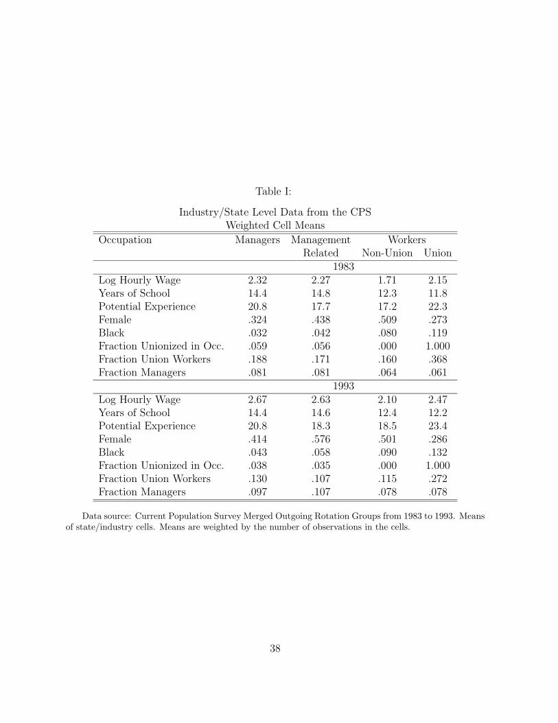
Table I:

Industry/State Level Data from the CPSWeighted Cell Means

Occupation Managers Management WorkersRelated Non-Union Union

1983Log Hourly Wage 2.32 2.27 1.71 2.15Years of School 14.4 14.8 12.3 11.8Potential Experience 20.8 17.7 17.2 22.3Female .324 .438 .509 .273Black .032 .042 .080 .119Fraction Unionized in Occ. .059 .056 .000 1.000Fraction Union Workers .188 .171 .160 .368Fraction Managers .081 .081 .064 .061

1993Log Hourly Wage 2.67 2.63 2.10 2.47Years of School 14.4 14.6 12.4 12.2Potential Experience 20.8 18.3 18.5 23.4Female .414 .576 .501 .286Black .043 .058 .090 .132Fraction Unionized in Occ. .038 .035 .000 1.000Fraction Union Workers .130 .107 .115 .272Fraction Managers .097 .107 .078 .078

Data source: Current Population Survey Merged Outgoing Rotation Groups from 1983 to 1993. Meansof state/industry cells. Means are weighted by the number of observations in the cells.

38

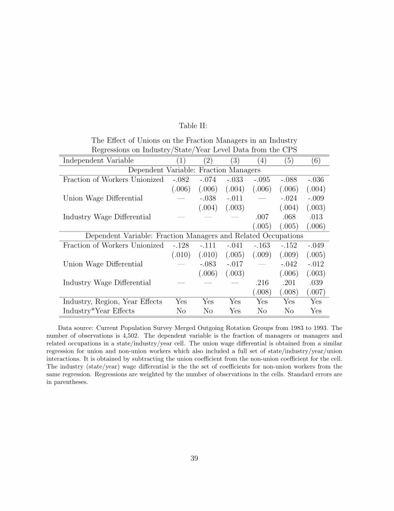
Table II:

The Effect of Unions on the Fraction Managers in an IndustryRegressions on Industry/State/Year Level Data from the CPS

Independent Variable (1) (2) (3) (4) (5) (6)Dependent Variable: Fraction Managers

Fraction of Workers Unionized -.082 -.074 -.033 -.095 -.088 -.036(.006) (.006) (.004) (.006) (.006) (.004)

Union Wage Differential — -.038 -.011 — -.024 -.009(.004) (.003) (.004) (.003)

Industry Wage Differential — — — .007 .068 .013(.005) (.005) (.006)

Dependent Variable: Fraction Managers and Related OccupationsFraction of Workers Unionized -.128 -.111 -.041 -.163 -.152 -.049

(.010) (.010) (.005) (.009) (.009) (.005)Union Wage Differential — -.083 -.017 — -.042 -.012

(.006) (.003) (.006) (.003)Industry Wage Differential — — — .216 .201 .039

(.008) (.008) (.007)Industry, Region, Year Effects Yes Yes Yes Yes Yes YesIndustry*Year Effects No No Yes No No Yes

Data source: Current Population Survey Merged Outgoing Rotation Groups from 1983 to 1993. Thenumber of observations is 4,502. The dependent variable is the fraction of managers or managers andrelated occupations in a state/industry/year cell. The union wage differential is obtained from a similarregression for union and non-union workers which also included a full set of state/industry/year/unioninteractions. It is obtained by subtracting the union coefficient from the non-union coefficient for the cell.The industry (state/year) wage differential is the the set of coefficients for non-union workers from thesame regression. Regressions are weighted by the number of observations in the cells. Standard errors arein parentheses.

39

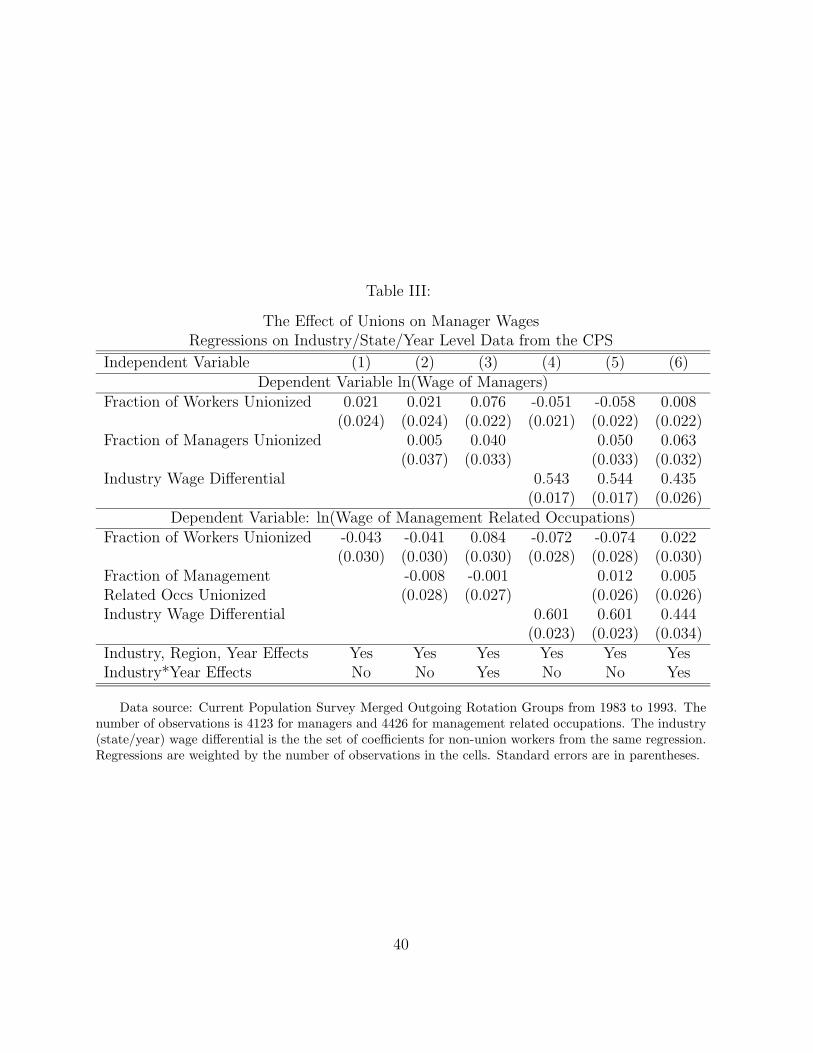
Table III:

The Effect of Unions on Manager WagesRegressions on Industry/State/Year Level Data from the CPS

Independent Variable (1) (2) (3) (4) (5) (6)Dependent Variable ln(Wage of Managers)

Fraction of Workers Unionized 0.021 0.021 0.076 -0.051 -0.058 0.008(0.024) (0.024) (0.022) (0.021) (0.022) (0.022)

Fraction of Managers Unionized 0.005 0.040 0.050 0.063(0.037) (0.033) (0.033) (0.032)

Industry Wage Differential 0.543 0.544 0.435(0.017) (0.017) (0.026)

Dependent Variable: ln(Wage of Management Related Occupations)Fraction of Workers Unionized -0.043 -0.041 0.084 -0.072 -0.074 0.022

(0.030) (0.030) (0.030) (0.028) (0.028) (0.030)Fraction of Management -0.008 -0.001 0.012 0.005Related Occs Unionized (0.028) (0.027) (0.026) (0.026)Industry Wage Differential 0.601 0.601 0.444

(0.023) (0.023) (0.034)Industry, Region, Year Effects Yes Yes Yes Yes Yes YesIndustry*Year Effects No No Yes No No Yes

Data source: Current Population Survey Merged Outgoing Rotation Groups from 1983 to 1993. Thenumber of observations is 4123 for managers and 4426 for management related occupations. The industry(state/year) wage differential is the the set of coefficients for non-union workers from the same regression.Regressions are weighted by the number of observations in the cells. Standard errors are in parentheses.

40

Table IV:

The Effect of Unions on CEO PayDependent Variable: Ln(Salary, Bonus and Other CEO Compensation)

Firm Level Regressions Using Bronars, Deere, and Tracy DataMean Full Manuf. Non-Manuf. Full Full Full

(Std. Dev.)Independent (1) (2) (3) (4) (5) (6)VariableFraction Union 0.319 -0.303 -0.186 -0.185 -0.120 0.015 0.252

(0.246) (0.054) (0.061) (0.095) (0.054) (0.058) (0.107)CEO Age 57.61 0.019 0.040 -0.048 -0.009 -0.007 -0.010

(5.872) (0.023) (0.023) (0.061) (0.023) (0.024) (0.031)CEO Age2/100 33.53 -0.015 -0.034 0.049 0.010 0.007 0.015

(6.769) (0.021) (0.020) (0.053) (0.020) (0.021) (0.027)CEO Tenure 7.655 0.018 0.021 0.023 0.016 0.020 0.020

(5.975) (0.006) (0.007) (0.010) (0.005) (0.005) (0.006)CEO Tenure 0.943 -0.032 -0.068 -0.015 -0.036 -0.053 -0.043

(1.752) (0.020) (0.027) (0.032) (0.019) (0.018) (0.019)New CEO 0.246 -0.064 -0.047 -0.107 -0.057 -0.065 -0.059

(0.431) (0.030) (0.031) (0.062) (0.026) (0.025) (0.021)Log Sales 7.885 0.148 0.230 0.153 0.236 0.187 -0.023

(1.000) (0.026) (0.026) (0.066) (0.040) (0.047) (0.080)Log Employment 3.185 0.176 0.035 0.190 0.043 0.090 0.362

(1.025) (0.025) (0.028) (0.056) (0.040) (0.047) (0.078)Stock Return 0.127 0.070 0.064 0.101 0.067 0.068 0.065

(0.871) (0.016) (0.016) (0.038) (0.014) (0.014) (0.014)Stock Return 0.270 0.017 0.020 0.003 0.018 0.023 0.017last period (1.505) (0.009) (0.011) (0.015) (0.009) (0.008) (0.011)Period (1974-1978) 0.332 0.322 0.360 0.197 0.319 0.330 0.336

(0.471) (0.035) (0.035) (0.077) (0.030) (0.028) (0.025)Period (1974-1978) 0.299 0.738 0.787 0.616 0.747 0.759 0.775

(0.458) (0.033) (0.033) (0.073) (0.029) (0.027) (0.027)Number of Observations 782 782 577 205 782 782 782Industry Effects No No No 44 103 NoFirm Effects No No No No No 327

Data sources: Unionization rates are from Bronars, Deere, and Tracy (1994), CEO pay data are fromKevin Murphy, all other variables are from Compustat. Data refer to four year aggregates for 1971-74,1975-78, and 1979-82. Standard errors are in parentheses.

41

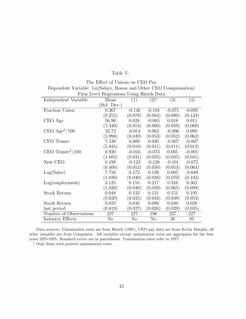
Table V:

The Effect of Unions on CEO PayDependent Variable: Ln(Salary, Bonus and Other CEO Compensation)

Firm Level Regressions Using Hirsch DataIndependent Variable Mean (1) (2)∗ (3) (4)

(Std. Dev.)Fraction Union 0.367 -0.146 -0.194 -0.075 -0.095

(0.255) (0.078) (0.084) (0.090) (0.124)CEO Age 56.96 0.028 -0.065 0.018 0.011

(5.330) (0.054) (0.060) (0.059) (0.069)CEO Age2/100 32.72 -0.014 0.062 -0.006 0.000

(5.998) (0.049) (0.053) (0.052) (0.062)CEO Tenure 7.538 0.000 0.020 -0.007 -0.007

(5.945) (0.010) (0.011) (0.011) (0.013)CEO Tenure2/100 0.920 -0.016 -0.073 0.005 -0.001

(1.882) (0.031) (0.035) (0.035) (0.041)New CEO 0.198 -0.123 -0.128 -0.101 -0.072

(0.400) (0.052) (0.050) (0.053) (0.064)Log(Sales) 7.756 0.172 0.139 0.005 -0.049

(1.030) (0.040) (0.038) (0.070) (0.103)Log(employment) 3.125 0.155 0.217 0.316 0.362

(1.020) (0.040) (0.039) (0.065) (0.099)Stock Return 0.048 0.132 0.131 0.151 0.195

(0.620) (0.035) (0.034) (0.038) (0.053)Stock Return 0.070 0.048 0.080 0.040 0.028last period (0.819) (0.027) (0.026) (0.029) (0.035)Number of Observations 227 227 196 227 227Industry Effects No No No 30 85

Data sources: Unionization rates are from Hirsch (1991), CEO pay data are from Kevin Murphy, allother variables are from Compustat. All variables except unionization rates are aggregates for the fouryears 1975-1978. Standard errors are in parentheses. Unionization rates refer to 1977.∗ Only firms with positive unionization rates.

42

Table VI:

The Effect of Unions on the Fraction Managers Across CountriesDependent Variable: Fraction Managers

Cross Country Panel Regressions

Full Full Full CanadaExcluded

Independent Variable (1) (2) (3) (4)Union Membership Rate -.052 -.049 .037 .000

(.047) (.050) (.050) (.026)Number of Observations 189 189 189 168Union Coverage Rate -.088 -.100 -.023 -.020

(.042) (.036) (.068) (.072)Number of Observations 28 28 28 25Time Dummies No Yes Yes YesCountry Dummies No No Yes Yes

Data sources: Data on Managerial Employment are from ILO. Unionization rates are from Visser(1997) with assistance from Danny Blanchflower and Michael Wallerstein. Coverage rates are from OECD(1994) and OECD (1997). Data refer to 16 countries for the membership data and 11 countries for thecoverage data and cover the years 1970 to 1993. Standard errors in parentheses are adjusted for groupingby country.

43

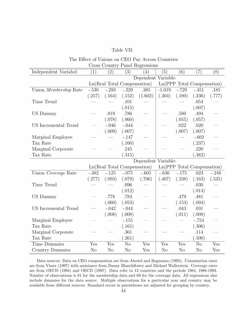
Table VII:

The Effect of Unions on CEO Pay Across CountriesCross Country Panel Regressions

Independent Variabel (1) (2) (3) (4) (5) (6) (7) (8)Dependent Variable:

Ln(Real Total Compensation) Ln(PPP Total Compensation)Union Membership Rate -.530 -.293 -.229 .385 -1.019 -.729 -.451 .185

(.257) (.164) (.152) (1.602) (.304) (.180) (.236) (.777)Time Trend — — .101 — — — .054 —

(.015) (.007)US Dummy — .819 .786 — — .580 .494 —

(.078) (.060) (.055) (.057)US Incremental Trend — -.046 -.044 — — .022 .020 —

(.009) (.007) (.007) (.007)Marginal Employee — — -.147 — — — -.602 —Tax Rate (.160) (.237)Marginal Corporate — — .245 — — — .220 —Tax Rate (.315) (.382)

Dependent Variable:Ln(Real Total Compensation) Ln(PPP Total Compensation)

Union Coverage Rate -.482 -.125 -.075 -.605 -.636 -.175 .023 -.248(.277) (.093) (.079) (.706) (.407) (.238) (.163) (.535)

Time Trend — — .096 — — — .030 —(.012) (.014)

US Dummy — .778 .783 — — .479 .481 —(.060) (.053) (.153) (.094)

US Incremental Trend — -.042 -.044 — — .043 .031 —(.008) (.008) (.011) (.008)

Marginal Employee — — -.155 — — — -.754 —Tax Rate (.161) (.306)Marginal Corporate — — .361 — — — .114 —Tax Rate (.261) (.500)Time Dummies Yes Yes No Yes Yes Yes No YesCountry Dummies No No No Yes No No No Yes

Data sources: Data on CEO compensation are from Abowd and Bognanno (1995). Unionization ratesare from Visser (1997) with assistance from Danny Blanchflower and Michael Wallerstein. Coverage ratesare from OECD (1994) and OECD (1997). Data refer to 12 countries and the periods 1984, 1988-1992.Number of observations is 81 for the membership data and 69 for the coverage data. All regressions alsoinclude dummies for the data source. Multiple observations for a particular year and country may beavailable from different sources. Standard errors in parentheses are adjusted for grouping by country.

44