unisa economic research working paper …uir.unisa.ac.za/bitstream/handle/10500/23509/chirwa &...
TRANSCRIPT

The Determinants Of Public Debt In The Euro Area: A Panel ARDL Approach
Themba Gilbert Chirwa
Nicholas M. Odhiambo
Working Paper 02/2018
January 2018
Themba Gilbert Chirwa
Department of Economics
University of South Africa
P. O. Box 392, UNISA
0003, Pretoria
South Africa
Email: [email protected] /
Nicholas M. Odhiambo
Department of Economics
University of South Africa
P. O. Box 392, UNISA
0003, Pretoria
South Africa
Email: [email protected] /
UNISA Economic Research Working Papers constitute work in progress. They are papers that are under submission or are
forthcoming elsewhere. They have not been peer-reviewed; neither have they been subjected to a scientific evaluation by an
editorial team. The views expressed in this paper, as well as any errors, omissions or inaccurate information, are entirely those
of the author(s). Comments or questions about this paper should be sent directly to the corresponding author.
©2018 by Dr Themba Gilbert Chirwa and Prof Nicholas M. Odhiambo
UNISA ECONOMIC RESEARCH
WORKING PAPER SERIES
Page | 1
The Determinants Of Public Debt In The Euro Area: A Panel ARDL Approach
Themba Gilbert Chirwa1 and Nicholas M. Odhiambo
Abstract
This study investigates the determinants of public debt in the EURO area that are either debt-
reducing or debt-creating using panel data from 10 European Countries. Using a panel ARDL
approach, the study results show that though the real interest rate – economic growth differential in
debt dynamics can be used to show whether debt is explosive or non-explosive, we find the speed of
adjustment to be a good predictor. The study results also reveal that while economic growth is debt-
reducing mainly in the short-run, the real exchange rate, investment, population growth are debt-
reducing in the long run. Similarly, though the real interest rate is debt-creating both in the short-
and long-run, government consumption is debt-creating in the long run while the relationship is
mixed in the short-run and differentiated across groups. These results have important policy
implications for the European Union. They include the need to continue having differentiated
Medium-Term Budgetary Objectives implemented across member states that focus on fiscal
sustainability as well as take into account all factors that may be debt-creating or debt-reducing.
Furthermore, there is need for European authorities to implement strategies that would encourage
lower or stable long-term interest rates as a strategy to reduce the accumulation of public debt in the
future.
Keywords: Euro Area; Panel ARDL Models; Cointegration; Public Debt
JEL Classification Code: C23, F34, H63, N14
1 Corresponding author: Dr Themba Gilbert Chirwa, Research Fellow, Department of Economics, University of South Africa (UNISA). Email address:

Page | 2
1. Introduction
Fiscal policy rules continue to play a major part of fiscal discipline in the European Union. There are
two explicit policy rules that were established in the Eurozone. The first rule is called the Excessive
Deficit Procedure (EDP) that was formulated under the Maastricht Treaty in 1993 and seeks to ensure
that each member state complies with fiscal budgetary discipline that endeavours to ensure that
member states’ fiscal deficits should not exceed 3% of GDP and the debt-to-GDP ratio should not
exceed 60% of GDP (European Commission 1997). The second rule under the European Union is the
Stability and Growth Pact (SGP) that defines the adoption of an even stricter fiscal rules which further
aim to strengthen the EDP when its rules are violated. The SGP has two regulations: first is called the
preventive arm of the SGP that seeks to strengthen surveillance of member states’ budgetary positions
which are expected to be not more than 0.5% of GDP when the EDP is violated; and the second is
the dissuasive arm of the SGP that focus on enforcing the implementation of the medium-term
budgetary objectives and issuance of penalties if the EDP continues to be violated by member states.
Under the SGP each member state that is regarded as being part of the preventive arm is expected to
implement medium-term budgetary objectives that would ensure governments maintain cyclically
adjusted budgetary positions that are close to a balanced budget, a fiscal deficit of not more than 0.5%
of GDP, or a budgetary surplus (European Commission 1997).
The goal of the EDP and SGP in the European Union is to ensure that Europe is able to create an
Economic and Monetary Union (EMU) that is characterised by a favourable macroeconomic
environment with low inflation, low interest rates, and fiscal sustainability where public expenditures
and debt are controlled. Empirical evidence has revealed that high government debt has four major
costs on the economy if not checked. Firstly, government debt has been found to be detrimental to

Page | 3
economic growth especially in situations where governments are forced to raise taxes in order meet
both their current and future debt obligations (Dotsey 1994). According to Krugman (1988), such tax
burdens end up creating policy and induced uncertainty thereby reducing consumption, disinvestment
and divestment. Secondly, other countries have experienced ineffective counter-cyclical fiscal
policies that lead to even deeper recessions (Aghion and Kharroubi 2007): one of the most recent
country affected is Venezuela that was hit by a major recession in 2014. Thirdly, countries that have
been ranked as high scrutiny economies by the International Monetary Fund (IMF) have to deal with
large fiscal consolidation policies that involve largely agonising restructuring of government
expenditures (Cochrane 2010). Fourthly, ineffective fiscal policies have exposed countries to even
greater sovereign risks as higher debt expose rollover risks due to high interest payments that crowd
out private investment and hence lead to default (Baldacci and Kumar 2010).
In this study we investigate two principle arguments. First, while the public debt dynamics have a
clear theoretical linkage on the public debt – economic growth nexus, the empirical linkage has not
been clear. In investigating public debt dynamics it is important to first start with the factors that are
included in the debt law of motion equation: these factors include the level of past debt, real interest
rate, real exchange rate, economic growth, and public balances. Second, because economic growth is
an endogenous variable, the factors that also impact economic growth are also likely to have a strong
long-run relationship with the accumulation of public debt. Some of the key macroeconomic variables
that have been augmented in the growth equation include investment, human capital stock, population
growth, government consumption, inflation, trade openness, among others (see Bosworth and Collins
2003; Chirwa and Odhiambo 2016, 2017 among others). In this case, the debt law of motion can also
be augmented with these extra regressors that affect economic growth.

Page | 4
According to the real interest rate – economic growth differential, real interest rates are positively
associated with debt accumulation whereas economic growth reduces debt over time. Furthermore,
public balances are negatively associated with debt accumulation: thus, a rise in public expenditures
relative to revenues collected is likely to increase public debt. In fact, this relationship is of particular
importance as Reinhart and Rogoff (2009) observed that the key drivers of debt accumulation over
time were not necessarily the costs of bailing out or recapitalizations during financial and economic
crises, but rather declining tax revenues as well as ambitious countercyclical fiscal policies adopted
by governments during recessions. The relationship between real exchange rate and debt can be
regarded as exhibiting threshold effects: debt is likely to increase if there is less than a complete pass-
through of exchange rate depreciation to inflation in the public debt dynamics. If there is less than a
complete exchange rate pass-through, then the real exchange rate is likely to be positively associated
with public debt. Conversely, if such a relationship does not hold, then the relationship between the
real exchange rate and public debt is likely to be negative as domestic currency denominated debt
would substitute foreign debt and hence lead to a decline in the debt-to-GDP ratio.
In order to investigate the automatic debt dynamics in the study countries we apply a panel
Autoregressive Distributed Lag (ARDL) method proposed by Pesaran et al. (1999). The contribution
of the study is therefore threefold. First, by using a panel ARDL model approach, the long-run level
relationships as well as the speed of adjustment (how fast a disequilibrium is corrected) in the debt
dynamic equation becomes of particular interest to the European Union as it relates to the viability of
the Stability and Growth Pact as well as fiscal sustainability. Second, given that the pooled mean
group estimation method allows for short-run coefficients to differ across groups, the results become
important particularly when designing country-specific medium-term budgetary objectives in order

Page | 5
to guide policymakers on what actions to take. Third, the augmented debt law of motion equation
adopted in this study is conditioned on other variables that will further assist policymakers in
understanding what other key macroeconomic variables can promote or hinder the accumulation of
debt.
The aim of the study therefore is to examine the key determinants of public debt in ten European
economies that are part of the EMU covering a period of 1970-2015. These countries include
Portugal, Greece, Spain, Italy, the United Kingdom, France, Belgium, Finland, Germany and Ireland.
These determinants are divided into two: debt-reducing and debt-creating variables. According to the
debt-law of motion, the debt-reducing variables include economic growth and the primary balance,
while debt-creating variables include the level of past debt and the real interest rate. We add more
variables to further investigate this relationship by including other equally important debt-reducing
variables such as investment, and population growth and debt-creating variables such as inflation and
real exchange rate depreciation.
The rest of the paper is planned as follows. Section 2 briefly reviews the literature and the key
macroeconomic trends in the study countries. Section 3 discuss the panel ARDL framework as well
as estimation techniques. Section 4 presents an empirical analysis of the regression results. Lastly,
section 5 provide conclusions and policy implications derived from the study.
2. Literature Review and Key Macroeconomic Trends
Most empirical research literature on automatic debt dynamics are done through debt sustainability
assessments to determine the level of financing required to reduce debt as well as to establish debt
limits. These assessments are conducted using specially designed debt sustainability tools that are

Page | 6
capable of conducting public and external debt sustainability analyses to identify, predict and provide
debt management solutions and prevent potential debt-related crises. Furthermore, such tools are
context-specific: one framework looks at debt management in market access countries (or MACs)
and represent advanced and emerging market countries that access their funds primarily through
international financial markets. The second debt management framework is used to assess debt
sustainability for all countries that are eligible for concessional financing such as those provided by
the World Bank and International Monetary Fund and the usual target is low-income countries (IMF
2013).
Debt sustainability analysis is important as it is capable of determining whether an economy has a
high probability that in the near future the accumulation of debt will remain stable or non-explosive
(Schumacher and Weder di Mauro 2015). However, such tools only provide an in-depth debt
sustainability analysis of a country’s debt stock and not necessarily determine the factors that are
debt-creating or debt-reducing. Second, much as such debt management frameworks are capable of
designing strategies to be adopted for debt to be non-explosive in the future, one fundamental flaw
of such debt sustainability frameworks is that they do not look at whether past debt sustainability
efforts were themselves sustainable or capable of returning back to its equilibrium path. As indicated
in the introduction section, the speed of adjustment towards the equilibrium path in dynamic models
thus becomes of paramount importance in predicting the future of debt management strategies.
Another inconvenience of such standardized debt sustainability frameworks is the need to switch
from debt sustainability tools for market access countries which are usually characterised by short-
term lending to debt sustainability tools designed for low-income economies that are subjected to
concessional financing. When advanced or emerging market economies face a crisis they are usually

Page | 7
subjected to crisis lending conditions that are highly concessional in nature (Schumacher and Weder
di Mauro 2015). As such, which tool to use and at what point becomes subjective and dependent on
the analyst.
The European Union member countries investigated in this study are categorised as being sanctioned
to be scrutinised under the preventive arm of the SGP. As of 2015, all countries had passed the 60%
debt-to-GDP threshold and thus subject to the implementation of Medium-Term Budgetary
Objectives aimed at reducing both fiscal deficits and the accumulation of public debt (European
Commission 1997; Eurostat 2017). The 2008-2009 financial crisis was the turning point for over half
of the study countries where the 60% debt-to-GDP threshold was violated with Finland having
reached this threshold in 2014 (Eurostat 2017). There are a number of macroeconomic factors that
have been highlighted through different studies in the economic literature for each member state.
In Portugal, the overall GDP growth trajectory was affected by high levels of corporate debt, slow-
moving investment opportunities, weak market perceptions that increased uncertainty, weak export
growth, and structural bottlenecks. Though the Portuguese authorities had set up an economic
recovery strategy that would see key fiscal consolidation strategies implemented such as a reduction
in the fiscal deficit to an average of 2.2% of GDP, this was ambitious given declining trends in GDP
growth as well as evolving expenditure pressures (IMF 2016a). Some critical areas that continued to
affect the fiscal balance included social benefits, pensions and public sector wages as well as a tax
policy that was unstable and unpredictable and hence not designed to encourage competitiveness and
hence economic growth. As for banks that were instrumental in contributing towards the financial
crisis continued to face weak balance sheets especially on non-performing loans, and corporate
governance issues related to lending procedures not guided by commercial criteria (IMF 2016a). The

Page | 8
real sector also continued to face some challenges related to structural bottlenecks that discouraged
competitiveness and economic growth: these were related particularly in the labour and product
markets that were affected by ineffective public institutions and high energy costs. Overall, concerns
about high debt levels still remain in Portugal as the level of public debt-to-GDP ratio continued to
rise from 84% of GDP in 2007 to 106% of GDP in 2015 (IMF 2016a; Eurostat 2017).
In Greece, the debt growth trajectory continues to be of great concern in the Euro area: before joining
the EMU in 1998 the economy had already hit the SGP debt-to-GDP threshold as debt levels had
risen to 95% of GDP which meant that Greece was already under high scrutiny and a candidate of
the preventive arm of the SGP. However, the debt growth trajectory continued to rise pre-financial
crisis of 2008 where it reached 107% of GDP in 2007. The trend further worsened during the post-
2008 financial crisis reaching its peak in 2014 at 180% of GDP (Eurostat 2017). There are number of
factors that were highlighted that may have affected this trajectory. The key challenge is that most of
Greece’s public debt is owned by its European counterparts: as such in order for Greece to restore its
medium term macroeconomic stability and economic growth and a return to market financing on a
sustainable basis there is need for Greece’s European partners to provide further debt relief to the
economy. This is very critical as the IMF has warned that without such debt relief Greece will be
unable to restore debt sustainability even if they implement fully the economic recovery program
(Schumacher and Weder di Mauro 2015; IMF 2010, 2017a). Other related structural reforms needed
as part of the economic recovery strategy include the need to broaden the income tax base, and fiscal
sustainability by reforming pension spending if Greece is to rebalance its fiscal budget towards either
a balanced budget or surplus. In the banking sector, Greece also continued to have high non-
performing loans and thus there is a need to relook at the lending procedures to ensure that they are
Page | 9
also guided by sound commercial principles (IMF 2017a). In the real sector, the economy still
continues to have restrictions that have impaired the investment climate: the product and service
markets continued to be protected and thus have affected job-creation initiatives in the economy (IMF
2017a).
In the Spanish economy, though there have been signs of economic recovery through improved fiscal
balances, real GDP growth, wage moderation, greater labour market flexibility, strengthening of
private sector balance sheets, and concerns of high debt-to-GDP levels continues to be significant
(IMF 2017b). As of 2007 Spain’s debt trajectory was stable averaging 36% of GDP: however, post-
2008 financial crisis the debt level almost doubled reaching 62% of GDP. The debt trajectory further
increased and had reached 100% as of 2015 (Eurostat 2017). The key downward risks that continue
to affect high debt levels in the economy include high public expenditures as well as a negative net
investment position. As such fiscal consolidation is required if debt sustainability is to be achieved
(IMF 2017b).
Italy continued to face slow economic growth as structural challenges remained significant in the
economy. Some of these challenges include very high non-performing loans that strained bank
balance sheets, high unemployment rate averaging 11%, high public debt that represented 132% of
GDP in 2015 thereby reaching a level that limits fiscal space that is allowable for countercyclical
fiscal policy to respond to adverse shocks. The economic recovery of Italy is thus expected to be
prolonged and subjected to further downward risks. The medium-term budgetary objectives are
therefore expected to be driven by structural reforms that focus on addressing bottlenecks related to
institutional, public administration, fiscal space with a focus on balanced budgets, labour market
inflexibility, pro-growth, distortive taxation, and banking sector challenges (IMF 2016b).
Page | 10
The United Kingdom (UK), though part of the European Union uses its own currency and is the
biggest financial hub of the EMU. However, though the UK is not part of the EMU, this means that
the implementation and adoption of the SGP is not relevant to the UK economy. Nevertheless, the
UK was not spared from the 2008 financial crisis. The UK is regarded as a high scrutiny country
having passed the debt-to-GDP threshold of 60%: the UK moved from 44% debt-to-GDP ratio in
2007 to 68% of GDP in 2009 (Eurostat 2017). This has been attributed to structural challenges
especially in the fiscal policy framework that contributed significantly to an excessive increase in
discretionary public spending (IMF 2011). The prominence of high public debt which reached 89%
of GDP in 2015 is deemed to threaten the UK’s future economic growth trajectory and lead to
crowding out effects of investment. The key structural reforms needed therefore have been aligned
towards ensuring financial sector reforms are implemented as well as prudent fiscal consolidation in
order to address fiscal imbalances (IMF 2011; Eurostat 2017).
France has also faced slow economic recovery and public debt still remains to be high. As of 2007,
France had already reached the 60% SGP threshold and the debt continued to rise reaching a debt-to-
GDP ratio of 96% as of 2015. Some of the challenges affecting such rise in debt has been attributed
to ineffective fiscal consolidation that stalled due to high public spending as well as irregular tax
revenues that were affected by high tax burdens (Eurostat 2017; IMF 2017c). France’s potential
economic growth continues to be constrained by low total factor productivity growth, a stagnant
working age population, high structural unemployment, weak external competitiveness, and firm-
level labour constraints. It is envisaged that if such structural bottlenecks are addressed there is a
likelihood of raising potential economic growth as well as boost employment (IMF 2017c).

Page | 11
Belgium has faced high public debt ratios as well beyond the 60% SGP threshold even before it joined
the EMU. Since the 1980s and till 2002, the average debt-to-GDP ratio averaged 115% of GDP per
annum before declining to 84% of GDP by 2007. During the post-2008 financial crisis, the debt levels
rose reaching its peak in 2015 at 106% of GDP (Eurostat 2017). As a result, Belgium continue to
experience slow growth and the major macroeconomic challenges attributed to such sluggish growth
have been high public debt due to increased public spending that continued to grow faster than GDP
as well as severe labour market fragmentation. Having qualified to be part of the preventive arm of
the SGP, there is need for a strong medium-term budgetary objective strategy that will ensure fiscal
consolidation targeting a balanced budget backed by efficiency-oriented structural reforms (IMF
2017d).
Similarly, Finland experienced a sluggish and fragile economy vulnerable to external downward
shocks during the study period. However, the debt performance in Finland has not been alarming
compared to other countries in the Eurozone: Finland had just reached the maximum debt-to-GDP
threshold of the SGP at 64% of GDP by 2015 (Eurostat 2017). The key drivers of such slow growth
include limited fiscal space, structural bottlenecks that have led to high labour costs, firm-level labour
constraints related to wage bargaining, as well as product market constraints in the retail and state
denominated sectors of the economy (IMF 2016c).
Prior to the 2008 financial crisis, Germany had already reached the debt ceiling threshold of the SGP
and in 2007 the debt-to-GDP ratio had reached 65% of GDP. Post-2008 financial crisis, the debt-to-
GDP ratio had reached 83% of GDP in 2010 (Eurostat 2017). However, the situation was reversed as
Germany under the preventive arm of the SGP commenced fiscal consolidation and since 2013 it has
recorded general government budget surpluses: this has made Germany to be back on a sustained

Page | 12
downward path which has seen its debt-to-GDP ratio declining to 71% of GDP as of 2015 (European
Commission 2017; Eurostat 2017).
Lastly, Ireland has been coined as Europe’s top growth performers that has been driven by strong
private consumption and a buoyant investment climate supported by construction in the real sector.
Furthermore, fiscal space has been very good with the government registering a fiscal surplus of 0.6%
of GDP in 2016. This contributed to a large extent towards reducing the debt-to-GDP ratio from 119%
of GDP in 2013 to 79% of GDP in 2015 (IMF 2017e; Eurostat 2017). Nevertheless, Ireland was one
of the countries in the world that was heavily hit by the 2008 financial crisis where the debt-to-GDP
ratio rose from 25% of GDP in 2007 and more than quadrupled reaching its maximum of 119% of
GDP by 2013. The large part of this public debt was to bailout the banking sector that had
accumulated a lot of non-performing loans as a result of the fallout of the construction burst (IMF
2017e; Eurostat 2017). As a result, continued fiscal consolidation is of fundamental importance if the
high debt-to-GDP ratio is to return back to its sustainable path. As of July 2017, the IMF forecasts on
public finances was expected to improve further with the structural deficit expected to meet the
medium-term budgetary objectives of the SGP of 0.5% of GDP (IMF 2017e).
3. Methodology and Estimation Techniques
According to the public debt dynamics, the debt law of motion equation assumes the following (Croce
and Juan-Ramon 2003; IMF 2013):
𝑑𝑡 = 𝑓(𝑑𝑡−1, 𝑔𝑡, 𝑟𝑡, 𝑝𝑏𝑡, 𝑟𝑒𝑟𝑡, 𝜋𝑡) (1)
From equation 1, debt is assumed to be a function of past debt, economic growth, real interest rate,
the primary balance, the real exchange rate and inflation. In the debt dynamics equation, past debt
Page | 13
and real interest rates are positively associated with the accumulation of debt while economic growth
and the primary balance are negatively associated with debt accumulation. The behaviour of the real
exchange rate, inflation and the accumulation of debt within the automatic debt dynamics is
ambiguous as they depend on the level of exchange rate pass-through achieved: thus, the impact can
be positive, negative or even insignificant if there is a complete pass-through or not. As earlier
indicated, the economic growth component is endogenous and hence the factors that affect economic
growth such as investment, population growth, government consumption, and trade openness, among
others, can also be included in the debt law of motion equation as additional explanatory variables
(see Fischer 1993; Bosworth and Collins 2003; Chirwa and Odhiambo 2016, 2017 among others).
In order to investigate this relationship, the study employs a pooled mean group estimation technique
based on the panel ARDL framework proposed by Pesaran et al. (1999). There are several reasons
for adopting this approach. Firstly, for the European Union SGP, models that ensure the fulfilment
of long-run homogeneity are of paramount importance to guarantee convergence on unified policies
adopted. This entails that the long-run level relationships between public debt and the regressors is
of importance as any arbitrage condition that is estimated will guide policymakers on how to
formulate long-term economic policies. Secondly, the short-run coefficients and error variances of
other explanatory variables used in a panel ARDL setting are assumed to be differentiated (Pesaran
et al. 1999) compared to panel fixed and random effects estimators that only allow the intercept to
differ across. This approach is important for the European Union especially when formulating
Medium-Term Budgetary Objectives for member states that qualify to be part of the preventive arm
of the SGP. Thirdly, the speed of adjustment can be used as an early sign of whether the future
direction of public debt is explosive or non-explosive: if the speed of adjustment or error correction

Page | 14
term is within the (0, -1) space, then the accumulation of future debt can be assumed to be non-
explosive; whereas if the speed of adjustment is not a subset of the (0, -1) benchmark then the
accumulation of future debt is deemed to be explosive or unstable. Finally, the panel ARDL
modelling approach corrects for endogeneity in the regressors through the inclusion of lags on short-
run coefficients that may differ across cross-sections.
Given this set-up, the panel 𝐴𝑅𝐷𝐿(p, q, q, … , q) debt law of motion equation can be presented as
follows:
𝑙𝑛𝐷𝐸𝐵𝑇𝑖𝑡 = 𝛽𝑖
+ ∑ 𝛽1,𝑖𝑗
𝑙𝑛𝐷𝐸𝐵𝑇𝑖,𝑡−𝑗
𝑝
𝑗=1
+ ∑ 𝛽2,𝑖𝑗
𝑞
𝑗=0
∆𝑙𝑛𝑌𝑖,𝑡−𝑗 + ∑ 𝛽3,𝑖𝑗
𝑞
𝑗=0
𝑙𝑛𝐼𝑁𝑉𝑖,𝑡−𝑗 + ∑ 𝛽4,𝑖𝑗
𝑞
𝑗=0
𝑙𝑛𝑃𝑂𝑃𝐺𝑖,𝑡−𝑗
+ ∑ 𝛽5,𝑖𝑗
𝑞
𝑗=0
𝑙𝑛𝐺𝐶𝑖,𝑡−𝑗 + ∑ 𝛽6,𝑖𝑗
𝑞
𝑗=0
𝑙𝑛𝑅𝐸𝑅𝑖,𝑡−𝑗 + ∑ 𝛽7,𝑖𝑗
𝑞
𝑗=0
𝑙𝑛𝑅𝐼𝑅𝑖,𝑡−𝑗 + ∑ 𝛽8,𝑖𝑗
𝑞
𝑗=0
𝑙𝑛𝐼𝑁𝐹𝐿𝑖,𝑡−𝑗
+ ∑ 𝛽9,𝑖𝑗
𝑞
𝑗=0
𝑙𝑛𝑇𝑅𝐴𝐷𝐸𝑖,𝑡−𝑗 + 𝜀𝑖𝑡 … … … … … … … … … … … … … … … … … … … … … … … … (2)
In equation 2, 𝛽𝑖 represents the fixed effects; while 𝛽1,𝑖𝑗, … , 𝛽9,𝑖𝑗 represent the coefficients of the
lagged dependent variable and regressors. In a panel error correction representation, equation (2) is
symbolised as follows:
∆𝑙𝑛𝐷𝐸𝐵𝑇𝑖𝑡 = 𝛽𝑖
+ ∑ 𝛽1,𝑖𝑗
∆𝑙𝑛𝐷𝐸𝐵𝑇𝑖,𝑡−𝑗
𝑝
𝑗=1
+ ∑ 𝛽2,𝑖𝑗
𝑞
𝑗=0
∆𝑙𝑛𝑌𝑖,𝑡−𝑗 + ∑ 𝛽3,𝑖𝑗
𝑞
𝑗=0
∆𝑙𝑛𝐼𝑁𝑉𝑖,𝑡−𝑗 + ∑ 𝛽4,𝑖𝑗
𝑞
𝑗=0
∆𝑙𝑛𝑃𝑂𝑃𝐺𝑖,𝑡−𝑗
+ ∑ 𝛽5,𝑖𝑗
𝑞
𝑗=0
∆𝑙𝑛𝐺𝐶𝑖,𝑡−𝑗 + ∑ 𝛽6,𝑖𝑗
𝑞
𝑗=0
∆𝑙𝑛𝑅𝐸𝑅𝑖,𝑡−𝑗 + ∑ 𝛽7,𝑖𝑗
𝑞
𝑗=0
∆𝑙𝑛𝑅𝐼𝑅𝑖,𝑡−𝑗 + ∑ 𝛽8,𝑖𝑗
𝑞
𝑗=0
∆𝑙𝑛𝐼𝑁𝐹𝐿𝑖,𝑡−𝑗
+ ∑ 𝛽9,𝑖𝑗
𝑞
𝑗=0
∆𝑙𝑛𝑇𝑅𝐴𝐷𝐸𝑖,𝑡−𝑗 + 𝛼1𝑙𝑛𝐷𝐸𝐵𝑇𝑖,𝑡−1 + 𝛼2,𝑖𝑗𝑙𝑛𝑌𝑖,𝑡−1 + 𝛼3,𝑖𝑗𝑙𝑛𝐼𝑁𝑉𝑖,𝑡−1 + 𝛼4,𝑖𝑗𝑙𝑛𝑃𝑂𝑃𝐺𝑖,𝑡−1
+ 𝛼5,𝑖𝑗𝑙𝑛𝐺𝐶𝑖,𝑡−1 + 𝛼6,𝑖𝑗𝑙𝑛𝑅𝐸𝑅𝑖,𝑡−1 + 𝛼7,𝑖𝑗𝑙𝑛𝐼𝑁𝐹𝑖,𝑡−1 + 𝛼8,𝑖𝑗𝑙𝑛𝑇𝑅𝐴𝐷𝐸𝑖,𝑡−1 + 𝜀𝑖𝑡 … … … … … … (3)

Page | 15
Equation (3) thus becomes the model used to test for no level relationship in a panel ARDL
framework. The parameters 𝛽1,𝑖𝑗, … , 𝛽9,𝑖𝑗 are short-run multipliers or elasticities and 𝛼1,𝑖𝑗, … , 𝛼8,𝑖𝑗
are the long-run multipliers (elasticities) used to calculate the error correction or speed of adjustment.
Once a long-run level relationship is known, the error correction model (ECM) in a panel ARDL
framework is estimated as follows:
∆𝑙𝑛𝐷𝐸𝐵𝑇𝑖𝑡 = 𝛽𝑖
+ ∑ 𝛽1,𝑖𝑗
∆𝑙𝑛𝐷𝐸𝐵𝑇𝑖,𝑡−𝑗
𝑝
𝑗=1
+ ∑ 𝛽2,𝑖𝑗
𝑞
𝑗=0
∆𝑙𝑛𝑌𝑖,𝑡−𝑗 + ∑ 𝛽3,𝑖𝑗
𝑞
𝑗=0
∆𝑙𝑛𝐼𝑁𝑉𝑖,𝑡−𝑗 + ∑ 𝛽4,𝑖𝑗
𝑞
𝑗=0
∆𝑙𝑛𝑃𝑂𝑃𝐺𝑖,𝑡−𝑗
+ ∑ 𝛽5,𝑖𝑗
𝑞
𝑗=0
∆𝑙𝑛𝐺𝐶𝑖,𝑡−𝑗 + ∑ 𝛽6,𝑖𝑗
𝑞
𝑗=0
∆𝑙𝑛𝑅𝐸𝑅𝑖,𝑡−𝑗 + ∑ 𝛽7,𝑖𝑗
𝑞
𝑗=0
∆𝑙𝑛𝑅𝐼𝑅𝑖,𝑡−𝑗 + ∑ 𝛽8,𝑖𝑗
𝑞
𝑗=0
∆𝑙𝑛𝐼𝑁𝐹𝐿𝑖,𝑡−𝑗
+ ∑ 𝛽9,𝑖𝑗
𝑞
𝑗=0
∆𝑙𝑛𝑇𝑅𝐴𝐷𝐸𝑖,𝑡−𝑗 + 𝜌𝑖𝐸𝐶𝑀𝑖,𝑡−1 + 𝜀𝑖𝑡 … … … … … … … … … … … … … … … … (4)
Pesaran et al. (1999) makes three critical assumptions when estimating a panel ARDL model. First,
the disturbance 𝜀𝑖𝑡 are independently and identically distributed across the countries and over time.
Second, the panel ARDL model follows a stationary process to guarantee that the coefficient of the
error correction term lies within the (0, -1) space: this is important in order to confirm that the long-
run relationship between the dependent variable and the explanatory variables exists. For this reason,
it is important to ensure that all variables of interest are either 𝐼(0) or 𝐼(1) variables. Third, the
pooled mean group or panel ARDL model assumes that there is long-run homogeneity where the
coefficients of all explanatory variables are similar across the cross-sections in the long run.
Finally, the study uses a number of data sources. Data on real GDP per capita, gross fixed capital
formation, government consumption, inflation, trade openness, nominal exchange rates, interest rates
was retrieved from the World Bank Development Indicators, 1970-2016 (World Bank 2017). Gross

Page | 16
government debt data was retrieved from the European Union AMECO database, 1970-2018
(European Union 2017) as well as the Eurostat database, 1970-2018 (Eurostat 2017). Data related to
the PPP conversion factor was retrieved from the World Economic Outlook database, 1980-2022
(IMF 2017f). From these databases, a full dataset containing annual time-series data was retrieved
covering the period 1970 – 20152. The following definition of the variables included were used: real
GDP per capita (real GDP expressed in 2010 constant USD prices as a share of population);
investment (proxied by gross fixed capital formation as a share of GDP); population growth (the
growth rate of population); government consumption share in GDP; gross government debt as a share
of GDP; the real exchange rate (ratio of the nominal exchange rate and PPP conversion factor for
GDP); inflation rate (growth rate of consumer price index); and international trade openness (proxied
by the sum of exports and imports as a share of GDP). A dummy variable that takes into account the
establishment of EMU in 1998 is also included to check if the study countries benefitted or were
made worse-off when the EMU was formed.
3.1 Panel-Based Stationarity Tests
The pooled mean group estimation methodology using a panel ARDL approach cannot be applied if
some variables are not integrated of order one or zero.
2 The study employs Eviews 9.5 for unit root tests and regression analysis.

Page | 17
Table 1: Stationarity Test for all Variables
Stationarity of all Variables in Levels Stationarity of all Variables in 1st Difference
Breitung (2000) Levin et al. (2002) Im et al. (2003) ADF pp Breitung (2000) Levin et al. (2002) Im et al. (2003) ADF pp
Variable Without
Trend
With
Trend
Without
Trend
With
Trend
Without
Trend
With
Trend
Without
Trend
With
Trend
Without
Trend
With
Trend
With
Trend
Without
Trend With Trend
Without
Trend
With
Trend
With
Trend
Without
Trend
With
Trend
Without
Trend
With
Trend
Log(RGDPC) - 0.81
[0.792]
0.38
[0.651] -
1.53
[0.938]
13.71
[0.844] -
4.06
[0.999] -
-2.72*
[0.003] -
-8.70*
[0.000] -
-9.63*
[0.000] -
127.4*
[0.000] -
214.1*
[0.000]
Log(INV) - - -1.41
[0.078] -
-1.38
[0.082] -
30.28
[0.065] -
14.54
[0.802] - - -
-11.25*
[0.000] -
-10.6*
[0.000] -
142.3*
[0.000] -
132.2*
[0.000] -
Log(POPG) - - -1.64** [0.050]
- -3.77* [0.000]
- 54.6*
[0.000] -
37.8* [0.009]
- - - - - - - - - - -
Log(GC) - 1.05
[0.855] -
-1.92**
[0.027]
- -1.34
[0.090] -
28.4
[0.100] -
22.2
[0.328] -
-5.66*
[0.000] -
-13.76*
[0.000] -
-11.7*
[0.000] -
153.1*
[0.000] -
152.9*
[0.000]
Log(DEBT) - 0.21
[0.586] -
-0.60
[0.273] -
0.48
[0.686] -
16.3
[0.697] -
12.1
[0.912] -
-6.30*
[0.000] -
-6.43*
[0.000] -
-7.86*
[0.000] -
99.8*
[0.000] -
86.7*
[0.000]
Log(RER) - -2.79*
[0.002] -
-1.01
[0.156] -
-0.85
[0.196] -
22.5
[0.313] -
15.5
[0.746] -
-14.15*
[0.000] -
-19.62*
[0.000] -
-16.1*
[0.000] -
216.3*
[0.000] -
215.6*
[0.000]
Log(RIR) - -
2.19**
[0.001]
- -0.01
[0.493] -
-0.31
[0.377] -
18.1
[0.576] -
22.8
[0.297] -
-11.16*
[0.000] -
-18.69*
[0.000] -
-18.5*
[0.000] -
259.6*
[0.000] -
271.8*
[0.000]
Log(INFL) - 1.75
[0.960] -
-2.76*
[0.002] -
-4.86*
[0.000] -
63.5*
[0.000] -
65.3*
[0.000] -
-6.18*
[0.000] -
-15.55*
[0.000] -
-17.0*
[0.000] -
235.2*
[0.000] -
500.0*
[0.000]
Log(TRADE) - -4.58* [0.004]
- -1.6** [0.045]
- -2.62* [0.004]
- 35.9** [0.015]
- 30.2
[0.065] -
-15.95* [0.000]
- -19.38* [0.000]
- -16.9* [0.000]
- 229.4* [0.000]
- 246.8* [0.000]
Note: for all p-values: * 1% significance level; ** 5% significance level.
Page | 18
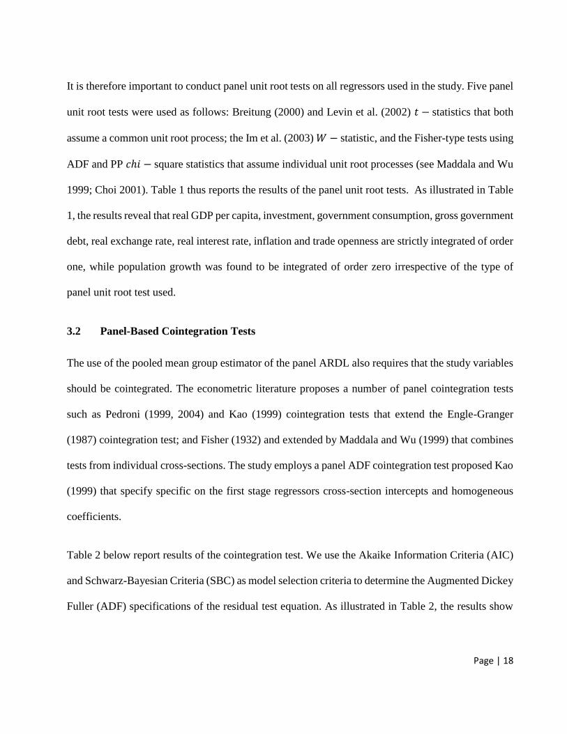
It is therefore important to conduct panel unit root tests on all regressors used in the study. Five panel
unit root tests were used as follows: Breitung (2000) and Levin et al. (2002) 𝑡 − statistics that both
assume a common unit root process; the Im et al. (2003) 𝑊 − statistic, and the Fisher-type tests using
ADF and PP 𝑐ℎ𝑖 − square statistics that assume individual unit root processes (see Maddala and Wu
1999; Choi 2001). Table 1 thus reports the results of the panel unit root tests. As illustrated in Table
1, the results reveal that real GDP per capita, investment, government consumption, gross government
debt, real exchange rate, real interest rate, inflation and trade openness are strictly integrated of order
one, while population growth was found to be integrated of order zero irrespective of the type of
panel unit root test used.
3.2 Panel-Based Cointegration Tests
The use of the pooled mean group estimator of the panel ARDL also requires that the study variables
should be cointegrated. The econometric literature proposes a number of panel cointegration tests
such as Pedroni (1999, 2004) and Kao (1999) cointegration tests that extend the Engle-Granger
(1987) cointegration test; and Fisher (1932) and extended by Maddala and Wu (1999) that combines
tests from individual cross-sections. The study employs a panel ADF cointegration test proposed Kao
(1999) that specify specific on the first stage regressors cross-section intercepts and homogeneous
coefficients.
Table 2 below report results of the cointegration test. We use the Akaike Information Criteria (AIC)
and Schwarz-Bayesian Criteria (SBC) as model selection criteria to determine the Augmented Dickey
Fuller (ADF) specifications of the residual test equation. As illustrated in Table 2, the results show

Page | 19
that the null hypothesis of no cointegration is rejected and conclude that the assumed debt dynamics
function used in this study is cointegrated at the 1% significance level regardless of the criteria used.
Table 2: Kao (1999) Panel Cointegration Test Results
Dependent
Variable
Selection
Criteria Lag-Length
ADF
(t-statistic) Co-integration Status
Log(DEBT) AIC ARDL (2,1,1,1,1,1,1,1,1) -4.07*
[0.000] Cointegrated
Log(DEBT) SBC ARDL (2,1,1,1,1,1,1,1,1) -4.35*
[0.000] Cointegrated
Null Hypothesis: No long-run relationships exist Note: for all p-values: * 1% significance level; ** 5% significance level; *** 10% significance level.
This proves that a long-run level relationship exists between gross government debt conditioned on
real GDP per capita, investment, population growth, government consumption, the real exchange
rate, the real interest rate, inflation, and trade openness Thus, we can proceed to use the pooled mean
group panel ARDL estimation method suggested by Pesaran et al. (1999) to investigate which factors
are debt-creating or debt-reducing.
4. Empirical Analysis of the Panel ARDL Regression Results
Debt sustainability analysis has been one of the important areas that is growing whereby studies are
conducted to understand the debt dynamics situation of countries especially factors that are debt-
creating and debt-reducing. Most importantly, open economy debt dynamics postulate that debt is a
function of economic growth, the real exchange rate, real interest rates, inflation, and public balances.
In this section, we extend this analysis by including other factors that especially have a direct impact
on economic growth and also check whether the theoretical predictions of debt dynamics as earlier
discussed apply in the Euro area. Table 3 summarises the PMG panel ARDL estimation results as
well as across groups’ estimation results on the relationship for the full sample period, 1970-2015.

Page | 20
Table 3: Pooled Mean Group Estimation Results – Full Sample (1970-2015)
Panel 1 – Estimated Long-Run Coefficients (Elasticities) [Dependent Variable: Log of Gross Government Debt log (𝐷𝐸𝐵𝑇)𝑡]
Regressor PMG Standard
Error t-statistic Probability Akaike Info. Criterion -2.903
log (𝑅𝐺𝐷𝑃)𝑡 -0.525 0.373 -1.406 0.160 Schwarz Criterion -1.753
log (𝑅𝐸𝑅)𝑡 -0.235** 0.108 -2.158 0.031 S.E. of Regression 0.057
log (𝑅𝐼𝑅)𝑡 2.352** 1.067 2.204 0.028 Residual Sum of Squares 1.097
log (𝐼𝑁𝐹𝐿)𝑡 -0.058 0.036 -1.585 0.1139
log (𝐼𝑁𝑉)𝑡 -0.578*** 0.345 -1.674 0.094
log (𝐺𝐶)𝑡 1.001* 0.391 2.555 0.011
log (𝑇𝑅𝐴𝐷𝐸)𝑡 -0.190 0.193 -0.986 0.324
log (𝑃𝑂𝑃𝐺)𝑡 -0.058* 0.020 -2.908 0.003
Panel 2 – Estimated Short-Run Coefficients (Elasticities) [Dependent Variable: change in log of Gross Government Debt log (𝐷𝐸𝐵𝑇)𝑡]
PMG Portugal Greece Spain Italy
United
Kingdom France Belgium Finland Germany Ireland
INT 0.360*
[0.002]
0.590**
[0.023]
0.029
[0.421]
-0.220***
[0.067]
1.151**
[0.032]
0.260**
[0.023]
0.334***
[0.053]
0.381*
[0.004]
0.246**
[0.011]
0.282*
[0.007]
0.547***
[0.056]
∆log (𝐷𝐸𝐵𝑇)𝑡−1 0.339*
[0.000]
0.0253*
[0.000]
-0.229*
[0.000]
0.439*
[0.000]
0.129*
[0.001]
0.608*
[0.000]
0.492*
[0.000]
0.579*
[0.000]
0.457*
[0.000]
0.399*
[0.000]
0.268*
[0.000]
∆log (𝑅𝐺𝐷𝑃)𝑡 -1.666*
[0.000]
-1.666*
[0.001]
-1.225*
[0.005]
-2.347*
[0.006]
-1.123*
[0.000]
-1.254*
[0.005]
-1.318
[0.326]
-1.113*
[0.004]
-3.485**
[0.017]
-1.848*
[0.004]
-1.279**
[0.020]
∆log (𝑅𝐸𝑅)𝑡 -0.008
[0.343]
-0.005*
[0.000]
-0.001*
[0.008]
-0.007*
[0.000]
0.001*
[0.000]
-0.012
[0.105]
0.009*
[0.001]
-0.004*
[0.000]
-0.052*
[0.000]
-0.051*
[0.000]
0.041
[0.148]
∆log (𝑅𝐼𝑅)𝑡 0.635**
[0.019]
0.862*
[0.001]
0.572**
[0.013]
0.378**
[0.016]
0.189*
[0.000]
-0.248*
[0.001]
0.322
[0.521]
0.546*
[0.002]
2.759***
[0.081]
1.119**
[0.044]
-0.149
[0.484]
∆log (𝐼𝑁𝐹𝐿)𝑡 0.016
[0.181]
0.033*
[0.000]
0.064*
[0.000]
0.073*
[0.000]
0.003*
[0.000]
-0.017*
[0.000]
-0.001*
[0.000]
0.029*
[0.000]
0.009*
[0.000]
0.035*
[0.000]
-0.061*
[0.000]
∆log (𝐼𝑁𝑉)𝑡 -0.030
[0.723]
-0.029
[0.328]
0.090**
[0.031]
-0.198**
[0.031]
-0.220*
[0.000]
-0.305*
[0.001]
-0.182
[0.329]
0.081**
[0.018]
0.463***
[0.069]
0.332**
[0.014]
-0.332*
[0.002]
∆log (𝐺𝐶)𝑡 0.121
[0.256]
0.061
[0.443]
0.234**
[0.016]
0.777*
[0.010]
-0.038***
[0.093]
-0.178**
[0.023]
-0.341
[0.520]
-0.227***
[0.059]
0.273
[0.576]
0.408**
[0.036]
0.239
[0.152]
∆log (𝑇𝑅𝐴𝐷𝐸)𝑡 0.049
[0.548]
-0.053***
[0.055]
-0.418*
[0.000]
0.023
[0.140]
0.089*
[0.000]
0.314*
[0.000]
0.043
[0.239]
-0.127*
[0.001]
0.436*
[0.009]
-0.089**
[0.017]
0.363*
[0.005]
∆log (𝑃𝑂𝑃𝐺)𝑡 -0.004
[0.710]
-0.021*
[0.000]
-0.029*
[0.000]
-0.064*
[0.000]
0.001*
[0.000]
0.007*
[0.000]
0.021*
[0.000]
-0.003*
[0.000]
0.063*
[0.000]
-0.013*
[0.000]
-0.001
[0.393]
DUM_EURO -0.046 [0.104]
-0.123* [0.000]
-0.028* [0.000]
0.021* [0.001]
-0.263* [0.000]
0.024* [0.000]
0.011* [0.000]
-0.058* [0.000]
-0.045* [0.000]
0.006* [0.000]
0.036* [0.000]
𝐸𝐶𝑀𝑡−1 -0.053*
[0.004]
-0.084*
[0.000]
0.011*
[0.001]
0.051*
[0.000]
-0.159*
[0.000]
-0.052*
[0.000]
-0.063*
[0.000]
-0.055*
[0.000]
-0.032*
[0.000]
-0.048*
[0.000]
-0.098*
[0.000]
Note: for all p-values: *** 1% significance level; ** 5% significance level; * 10% significance level.
Page | 21
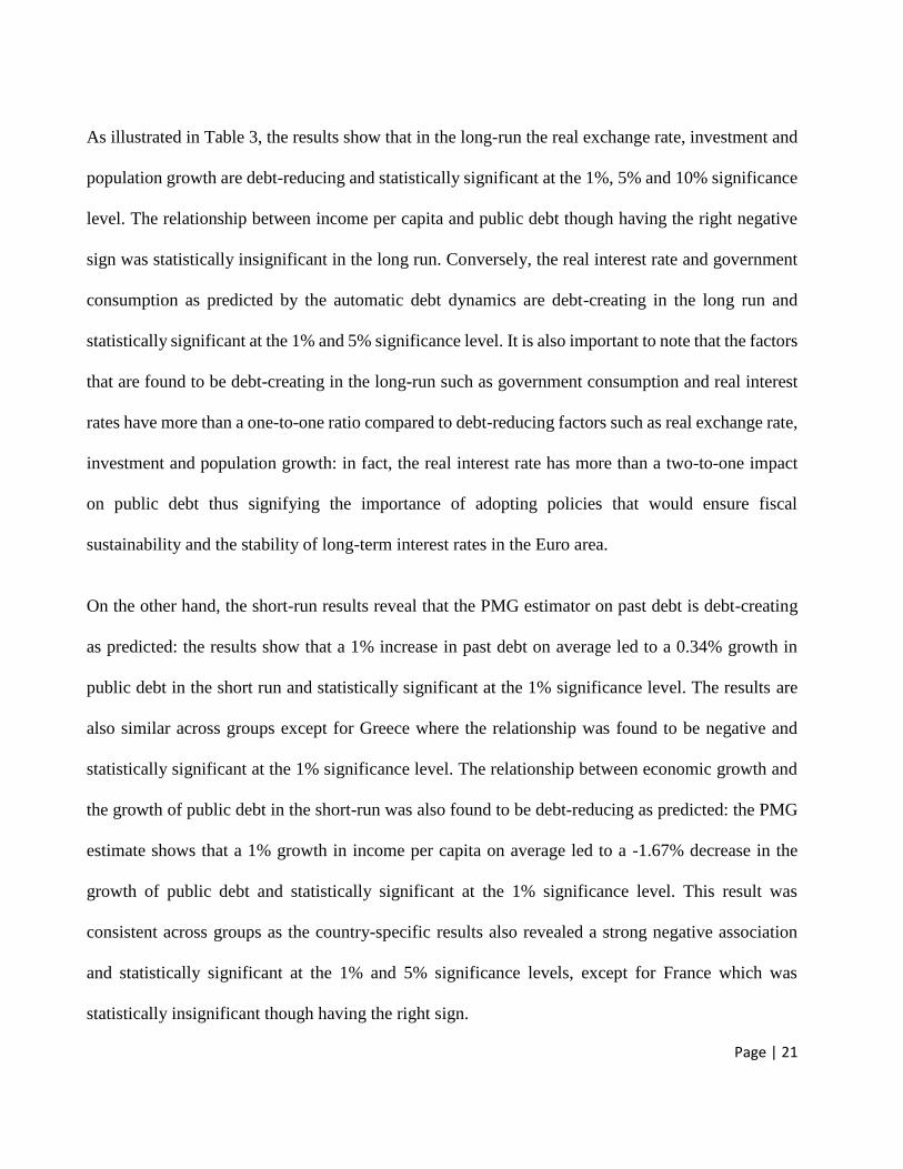
As illustrated in Table 3, the results show that in the long-run the real exchange rate, investment and
population growth are debt-reducing and statistically significant at the 1%, 5% and 10% significance
level. The relationship between income per capita and public debt though having the right negative
sign was statistically insignificant in the long run. Conversely, the real interest rate and government
consumption as predicted by the automatic debt dynamics are debt-creating in the long run and
statistically significant at the 1% and 5% significance level. It is also important to note that the factors
that are found to be debt-creating in the long-run such as government consumption and real interest
rates have more than a one-to-one ratio compared to debt-reducing factors such as real exchange rate,
investment and population growth: in fact, the real interest rate has more than a two-to-one impact
on public debt thus signifying the importance of adopting policies that would ensure fiscal
sustainability and the stability of long-term interest rates in the Euro area.
On the other hand, the short-run results reveal that the PMG estimator on past debt is debt-creating
as predicted: the results show that a 1% increase in past debt on average led to a 0.34% growth in
public debt in the short run and statistically significant at the 1% significance level. The results are
also similar across groups except for Greece where the relationship was found to be negative and
statistically significant at the 1% significance level. The relationship between economic growth and
the growth of public debt in the short-run was also found to be debt-reducing as predicted: the PMG
estimate shows that a 1% growth in income per capita on average led to a -1.67% decrease in the
growth of public debt and statistically significant at the 1% significance level. This result was
consistent across groups as the country-specific results also revealed a strong negative association
and statistically significant at the 1% and 5% significance levels, except for France which was
statistically insignificant though having the right sign.
Page | 22
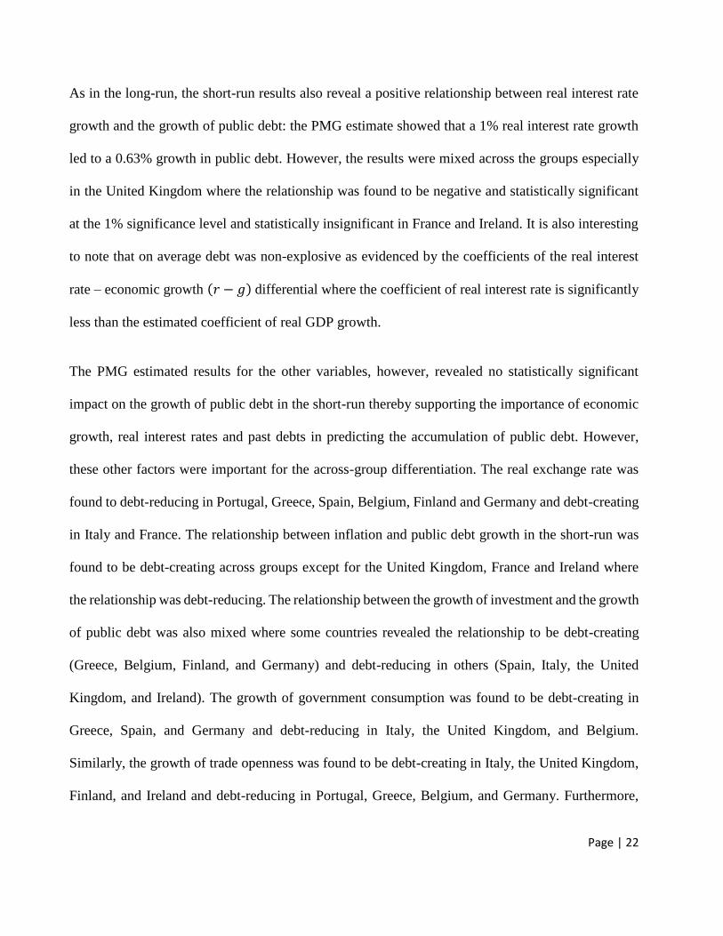
As in the long-run, the short-run results also reveal a positive relationship between real interest rate
growth and the growth of public debt: the PMG estimate showed that a 1% real interest rate growth
led to a 0.63% growth in public debt. However, the results were mixed across the groups especially
in the United Kingdom where the relationship was found to be negative and statistically significant
at the 1% significance level and statistically insignificant in France and Ireland. It is also interesting
to note that on average debt was non-explosive as evidenced by the coefficients of the real interest
rate – economic growth (𝑟 − 𝑔) differential where the coefficient of real interest rate is significantly
less than the estimated coefficient of real GDP growth.
The PMG estimated results for the other variables, however, revealed no statistically significant
impact on the growth of public debt in the short-run thereby supporting the importance of economic
growth, real interest rates and past debts in predicting the accumulation of public debt. However,
these other factors were important for the across-group differentiation. The real exchange rate was
found to debt-reducing in Portugal, Greece, Spain, Belgium, Finland and Germany and debt-creating
in Italy and France. The relationship between inflation and public debt growth in the short-run was
found to be debt-creating across groups except for the United Kingdom, France and Ireland where
the relationship was debt-reducing. The relationship between the growth of investment and the growth
of public debt was also mixed where some countries revealed the relationship to be debt-creating
(Greece, Belgium, Finland, and Germany) and debt-reducing in others (Spain, Italy, the United
Kingdom, and Ireland). The growth of government consumption was found to be debt-creating in
Greece, Spain, and Germany and debt-reducing in Italy, the United Kingdom, and Belgium.
Similarly, the growth of trade openness was found to be debt-creating in Italy, the United Kingdom,
Finland, and Ireland and debt-reducing in Portugal, Greece, Belgium, and Germany. Furthermore,

Page | 23
the relationship between population growth and the growth of public debt was also mixed: the
relationship was found to be debt-creating in Italy, the United Kingdom, France, and Finland, and
debt-reducing in Portugal, Greece, Spain, Belgium and Germany. Lastly, the establishment of the
EMU was found to be debt-reducing for countries such as Portugal, Greece, Italy, Belgium and
Finland, and debt-creating for Spain, the United Kingdom, France, Germany and Ireland. All results
were statistically significant at the 1% significance level in these countries.
As regards the speed of adjustment, the ECM coefficient has the right negative sign and within the
(0,-1) space and statistically significant at the 1% significance level, except in Greece and Spain
where the error correction term, though close to zero, were positive. This implies that the
accumulation of debt was non-explosive in Portugal, Italy, the United Kingdom, France, Belgium,
Finland, Germany and Ireland and relatively explosive in Greece and Spain. However, some caution
should be taken here. Schumacher and Weder di Mauro (2015) note that in May 2010 the IMF granted
a stand-by arrangement to Greece worth €30 billion which was more than 3,000% of its allocated
quota. The criteria used for granting such access to financing was the debt sustainability assessment
on the baseline scenario that the IMF projected: according to their estimates, the debt-to-GDP ratio
was projected to peak in 2013 at 149% of GDP and thereafter a gradual decline to 120% by 2020
though compounded by a number of downward risks and uncertainties to guarantee with a high
probability that such a scenario would be met (IMF 2010). Unfortunately, the debt-to-GDP ratio
reached 177% of GDP by 2013, peaked at 180% of GDP in 2014 before declining back to 177% of
GDP in 2015 (Eurostat 2017).
Using the panel ARDL approach adopted in this paper, we investigate as to whether the speed of
adjustment for Greece and the other study countries could have forewarned the IMF before such a

Page | 24
decision was made in May 2010 by simply running a regression for the subsequent periods
commencing 1970-2005 to the full sample period, 1970-2015 and observing the trends in the speed
of adjustment. We divide the countries into three categories. The first category represent member
states that experienced a speed of adjustment that was outside the unit circle and hence regarded as
unsustainable at some point: according to our results, these countries include Portugal, Greece and
Spain and the results are depicted in Figure 1. The second category of countries include those whose
speed of adjustment was within the unit circle but showed signs of slowing over time representing
member states with relatively high probability of debt becoming unsustainable: based on our results,
these countries include Italy, Ireland and Finland and the results are depicted in Figure 2. The third
category represents member states with relatively low probability of debt becoming unsustainable
whose speed of adjustment was close to lower band of the (0, -1) space which means that the model
returned back to the equilibrium path relatively quickly towards its equilibrium path when subjected
to a shock and thus having a low probability of non-explosive debt: according to the results, these
countries include Germany, the United Kingdom, Belgium and France and the results are depicted in
Figure 3.
Though we do not provide full regression results due to limited space in this paper, the trends in the
speed of adjustment for the three categories are outlined in Figures 1-3. As illustrated in Figure 1,
given that the speed of adjustment was consistently negative and within the (0, -1) threshold, our
results concur with the IMF observation that debt was sustainable or non-explosive in Greece between
2005 to 2009 and 2010 to 2014 and only became explosive in 2015 with a positive speed of
adjustment.

Page | 25
Figure 1: Trends in Speed of Adjustment – Portugal, Greece and Spain
Figure 2: Trends in Speed of Adjustment – Italy, Ireland and Finland
Figure 3: Trends in Speed of Adjustment – Germany, UK, Belgium and France
Source: Author Calculations in Eviews 9.5
(0.20)
(0.15)
(0.10)
(0.05)
-
0.05
0.10
1970-2005 1970-2006 1970-2007 1970-2008 1970-2009 1970-2010 1970-2011 1970-2012 1970-2013 1970-2014 1970-2015
Speed of Adjustment
Portugal Greece Spain
(0.35)
(0.30)
(0.25)
(0.20)
(0.15)
(0.10)
(0.05)
-
1970-2005 1970-2006 1970-2007 1970-2008 1970-2009 1970-2010 1970-2011 1970-2012 1970-2013 1970-2014 1970-2015
Speed of Adjustment
Italy Ireland Finland
(0.07)
(0.06)
(0.05)
(0.04)
(0.03)
(0.02)
(0.01)
-
1970-2005 1970-2006 1970-2007 1970-2008 1970-2009 1970-2010 1970-2011 1970-2012 1970-2013 1970-2014 1970-2015
Speed of Adjustment
Germany UK Belgium France

Page | 26
Based on the 2015 outcome where the speed of adjustment was outside the unit circle, out study
results support the IMF’s request for debt relief to be granted to Greece from its European partners if
debt sustainability is to be restored (IMF 2017a). As for Spain, the positive speed of adjustment result
in 2015 provides a sign that indeed debt levels are also becoming unsustainable having reached a
debt-to GDP ratio of 100% in the same year. Comparing the speed of adjustment between Greece and
Spain, we conclude that Spain had a higher probability of debt being unsustainable compared to
Greece during the period 2005-2015.
Therefore, Spain’s Medium-Term Budgetary Objectives should focus on ensuring that fiscal
consolidation is implemented with a focus on reducing public expenditures as well as improving the
negative net investment position if debt sustainability is to be achieved (IMF 2017b). Similarly, for
Portugal, the speed of adjustment was violated in 2014 when debt had reached 131% of GDP and
thus fiscal sustainability strategies are also crucial to ensure that debt becomes stable or is reduced in
the future.
As for Italy, Ireland and Finland, their debt levels presented a high probability of risk of debt
becoming unsustainable especially from 2013 onwards and the likelihood with a high probability
being depicted in Finland. For Germany, the UK, Belgium and France, the trends in the speed of
adjustment remain relatively low meaning that any shock to debt dynamics will quickly return back
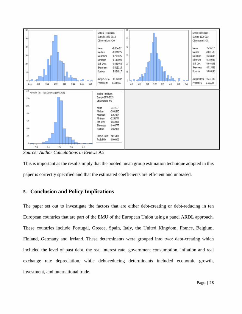
to its equilibrium path. Finally, the panel ARDL model assumes that the error terms are independently
and identically distributed. Thus, Figure 4 presents the distribution of the estimated residuals from
the subsamples as well as the full sample and confirm that they are all normally distributed.

Page | 27
Figure 4: Normality Tests
0
10
20
30
40
50
60
-0.20 -0.15 -0.10 -0.05 0.00 0.05 0.10 0.15
Series: Residuals
Sample 1970 2005
Observations 340
Mean -8.77e-17
Median -0.000765
Maximum 0.169922
Minimum -0.205287
Std. Dev. 0.043088
Skewness 0.064020
Kurtosis 5.789362
Jarque-Bera 110.4566
Probability 0.000000 0
10
20
30
40
50
60
-0.20 -0.15 -0.10 -0.05 0.00 0.05 0.10 0.15
Series: Residuals
Sample 1970 2006
Observations 350
Mean -6.27e-17
Median -0.000746
Maximum 0.187659
Minimum -0.207737
Std. Dev. 0.043748
Skewness 0.063873
Kurtosis 5.928048
Jarque-Bera 125.2677
Probability 0.000000
0
20
40
60
80
100
120
-0.20 -0.15 -0.10 -0.05 0.00 0.05 0.10 0.15 0.20
Series: Residuals
Sample 1970 2007
Observations 360
Mean -1.26e-16
Median -0.000792
Maximum 0.198098
Minimum -0.209753
Std. Dev. 0.043491
Skewness 0.105418
Kurtosis 6.028605
Jarque-Bera 138.2535
Probability 0.000000
0
20
40
60
80
100
120
-0.2 -0.1 0.0 0.1 0.2
Series: Residuals
Sample 1970 2008
Observations 370
Mean -9.16e-17
Median -0.001414
Maximum 0.200818
Minimum -0.207788
Std. Dev. 0.045605
Skewness 0.314816
Kurtosis 6.003143
Jarque-Bera 145.1526
Probability 0.000000
0
20
40
60
80
100
120
-0.2 -0.1 0.0 0.1 0.2
Series: Residuals
Sample 1970 2009
Observations 380
Mean 3.61e-17
Median -0.001652
Maximum 0.208025
Minimum -0.213608
Std. Dev. 0.045490
Skewness 0.272036
Kurtosis 6.486258
Jarque-Bera 197.1252
Probability 0.000000
0
20
40
60
80
100
120
-0.2 -0.1 0.0 0.1 0.2
Series: Residuals
Sample 1970 2010
Observations 390
Mean -2.23e-16
Median -0.002975
Maximum 0.214217
Minimum -0.216883
Std. Dev. 0.047656
Skewness 0.447276
Kurtosis 5.940579
Jarque-Bera 153.5175
Probability 0.000000
0
20
40
60
80
100
120
-0.2 -0.1 0.0 0.1 0.2
Series: Residuals
Sample 1970 2011
Observations 400
Mean 1.05e-16
Median -0.002729
Maximum 0.212928
Minimum -0.217917
Std. Dev. 0.047492
Skewness 0.415036
Kurtosis 5.884629
Jarque-Bera 150.1684
Probability 0.000000
0
20
40
60
80
100
120
-0.2 -0.1 0.0 0.1 0.2
Series: Residuals
Sample 1970 2012
Observations 410
Mean 1.28e-17
Median -0.002307
Maximum 0.214658
Minimum -0.223458
Std. Dev. 0.047758
Skewness 0.314499
Kurtosis 5.634586
Jarque-Bera 125.3350
Probability 0.000000
Page | 28
0
10
20
30
40
50
60
-0.15 -0.10 -0.05 0.00 0.05 0.10 0.15 0.20
Series: Residuals
Sample 1970 2013
Observations 420
Mean -1.80e-17
Median -0.001225
Maximum 0.206625
Minimum -0.148594
Std. Dev. 0.046463
Skewness 0.513115
Kurtosis 5.064617
Jarque-Bera 93.02632
Probability 0.000000 0
10
20
30
40
50
60
-0.15 -0.10 -0.05 0.00 0.05 0.10 0.15 0.20
Series: Residuals
Sample 1970 2014
Observations 430
Mean 2.43e-17
Median -0.001585
Maximum 0.203646
Minimum -0.150233
Std. Dev. 0.046291
Skewness 0.513838
Kurtosis 5.066196
Jarque-Bera 95.41139
Probability 0.000000
0
20
40
60
80
100
120
140
-0.2 -0.1 0.0 0.1 0.2
Series: Residuals
Sample 1970 2015
Observations 440
Mean 1.47e-17
Median -0.001840
Maximum 0.267352
Minimum -0.230747
Std. Dev. 0.049998
Skewness 0.466777
Kurtosis 6.562003
Jarque-Bera 248.5888
Probability 0.000000
Normality Test - Debt Dynamics (1970-2015)
Source: Author Calculations in Eviews 9.5
This is important as the results imply that the pooled mean group estimation technique adopted in this
paper is correctly specified and that the estimated coefficients are efficient and unbiased.
5. Conclusion and Policy Implications
The paper set out to investigate the factors that are either debt-creating or debt-reducing in ten
European countries that are part of the EMU of the European Union using a panel ARDL approach.
These countries include Portugal, Greece, Spain, Italy, the United Kingdom, France, Belgium,
Finland, Germany and Ireland. These determinants were grouped into two: debt-creating which
included the level of past debt, the real interest rate, government consumption, inflation and real
exchange rate depreciation, while debt-reducing determinants included economic growth,
investment, and international trade.

Page | 29
The debt dynamics debate state that the real interest rate – economic growth differential is perhaps
the most important relationship that will determine whether a country’s debt is explosive or non-
explosive. This is one of the indicators if a country is to be deemed solvent or financially sustainable.
The empirical results in this study have shown that the relationship between past debt and present
debt is largely positive and significantly associated in all countries as predicted, except Greece where
the relationship was found to be negative and statistically significant. Similarly, economic growth
revealed a negative relationship in all the countries as predicted, except in France where the
relationship was insignificant though having the right sign. Conversely, the relationship between the
real interest rate and the accumulation of debt was found to be positive and significantly associated
in all countries both in the short- and long-run as predicted, except in the United Kingdom where the
relationship was found to be negative and statistically significant in the short run.
What is interesting to note in this study is that the coefficient on the economic growth variable was
greater than the coefficient of the real interest rate regardless of whether the coefficient was
statistically significant or not implying that the (𝑟 − 𝑔) differential is negative in all study countries
and thus debt could be considered as non-explosive. However, much as this differential is important
in theoretical and empirical debt dynamics to show whether debt is non-explosive or explosive in the
long-run, we propose the use of the speed of adjustment as an appropriate measure of this relationship.
The evidence presented in this paper has shown that much as the real interest rate – economic growth
differential was consistently in favour of non-explosive debt in the study countries, the speed of
adjustment for Portugal, Greece and Spain revealed an unstable debt trajectory when a subsample
and a full sample were considered.

Page | 30
In general, the results also show that the impact of the other explanatory variables were largely
insignificant based on pooled data though mixed when country-specific results were considered. The
results based on the pooled mean group estimator revealed that while government consumption was
debt-creating and the real exchange rate, investment and population growth debt-reducing in the long
run, the real exchange rate, inflation, investment, government consumption, trade openness,
population growth, and the establishment of the EMU had no significant impact in the short-run.
However, the following important results were revealed when country-specific results were
considered in the short run: inflation was found to be debt-creating in all countries except the United
Kingdom, France, and Ireland where inflation was debt-reducing. Investment was found to be debt-
reducing in Spain, Italy, the United Kingdom, and Ireland; and debt-creating in Greece, Belgium,
Finland, and Germany. Government consumption was found to be debt-creating in Greece, Spain,
and Germany; and debt-reducing in Italy, the United Kingdom, and Belgium. Trade openness was
found to be debt-reducing in Portugal, Greece, Belgium, and Germany; and debt-creating in Portugal,
Greece, Belgium and Germany; and debt-creating in Italy, the United Kingdom, Finland, and Ireland.
The results also showed that population growth was debt-reducing in Portugal, Greece, Spain,
Belgium and Ireland; and debt-creating in Italy, the United Kingdom, France, and Finland; and debt-
reducing in Portugal, Greece, Spain, Belgium and Germany. Last but not least, the establishment of
the EMU was debt-reducing for Portugal, Greece, Italy, Belgium, and Finland; and debt-creating for
Spain, the United Kingdom, France, Germany and Ireland.
These results have significant policy implications especially for the EMU and in particular what other
factors to consider when developing Medium-Term Budgetary Objectives (MTOs) for various
countries. Though there are many recommendations to be made from the study results, we emphasize

Page | 31
on three major ones. First, we find the speed of adjustment to be a better predictor of whether debt is
explosive or non-explosive in the future compared to using the real interest rate – economic
differential. Second, the study results have revealed that different variables can affect the
accumulation of debt differently across groups. In particular, variables that are thought to be debt-
creating in some countries are in fact debt-reducing in others. Hence, a ‘one-size-fits-all’ policy is not
a good strategy to implement in the Euro zone. An analytical framework proposed in this paper would
be a first step towards understanding what either stimulates or hinders the accumulation of debt both
in the short- and long-run. Third, the study also revealed that in fact the real interest rate and
government consumption have a huge impact in terms of debt-creation compared to other factors and
as such policies that will contribute towards lowering long-term interest rates as well as fiscal
sustainability should be also be encouraged in the study countries in the long run.
References
Baldacci E, Kumar MS (2010) Fiscal Deficits, Public Debt and Sovereign Bond Yields, IMF Working
Paper, WP/10/184: 1-28.
Bosworth B, Collins S (2003) The Empirics of Growth: An update. Brookings Papers on Economic
Activity, 2: 113-206.
Breitung J (2000) The Local Power of Some Unit Root Tests for Panel Data. In B. Baltagi (Ed.),
Advances in Econometrics, Vol. 15: Nonstationary Panels, Panel Cointegration, and Dynamic
Panels, Amsterdam: JAI Press: p. 161–178.
Chirwa TG, Odhiambo NM (2016) What Drives Long-Run Economic Growth? Empirical evidence
from South Africa. Economia Internazionale/International Economics, 69(4): 425-452.
Chirwa TG, Odhiambo NM (2017) Sources of Economic Growth in Zambia: An empirical
investigation. Global Business Review 18(2): 275-290

Page | 32
Choi I (2001) Unit Root Tests for Panel Data. Journal of International Money and Finance, 20: 249-
272.
Croce E, Juan-Ramon H (2003) Assessing Fiscal Sustainability: A cross-country comparison. IMF
Working Paper, WP/03/145: 1-33.
Engle RF, Granger CWJ (1987) Co-integration and Error-Correction: Representation, estimation, and
testing. Econometrica 55(2): 251–276.
European Commission (1997) Strengthening of the Surveillance of Budgetary Positions and the
Surveillance and Coordination of Economic Policies. Council Regulation (EC) No. 1466/97.
European Commission (2017) Assessment of the 2017 Stability Programme for Germany. Brussels,
May 23. Retrieved from https://ec.europa.eu/info/sites/info/files/05_de_sp_assessment.pdf
European Union (2017) AMECO Database on Gross Public Debt. Retrieved from
http://ec.europa.eu/economy_finance/ameco/user/serie/SelectSerie.cfm
Eurostat (2017) Database on Gross Public Debt. Retrieved from https://ec.europa.eu/info/business-
economy-euro/indicators-statistics/economic-databases/macro-economic-database-
ameco/download-annual-data-set-macro-economic-database-ameco_en
Fisher RA (1932) Statistical Methods for Research Workers. 4th Edition, Edinburgh: Oliver & Boyd.
Fischer S (1993) The Role of Macroeconomic Factors in Growth. Journal of Monetary Economics
32(3): 485-512.
Im KS, Pesaran MH, Shin Y (2003) Testing for Unit Roots in Heterogeneous Panels. Journal of
Econometrics, 115: 53–74.
International Monetary Fund (2010) Greece: Staff Report Request for Stand-By Arrangement. IMF
Country Report No. 10/110, May.
_______________________ (2011) United Kingdom Sustainability Report. Report 9 of 10.
Retrieved from https://www.imf.org/external/np/country/2011/mapuk.pdf
_______________________ (2013) Staff Guidance Note for Public Debt Sustainability Analysis in
Market Access Countries, Strategy, Policy and Review Department, May 9. Retrieved from
http://www.imf.org/external/np/pp/eng/2013/050913.pdf
_______________________ (2016a) Portugal 2016 Article IV Consultation – Press Release; Staff
Report; and Statement by the Executive Director for Portugal. IMF Country Report No.
16/300, September.

Page | 33
_______________________ (2016b) Italy 2016 Article IV Consultation – Press Release; Staff
Report; and Statement by the Executive Director for Italy. IMF Country Report No. 16/222,
July.
_______________________ (2016c) Finland 2016 Article IV Consultation – Press Release; Staff
Report; and Statement by the Executive Director for Finland. IMF Country Report No.
16/368, November.
_______________________ (2017a) Greece Request for Stand-By Arrangement – Press Release;
Staff Report; and Statement by the Executive Director for Greece. IMF Country Report No.
17/229, July.
_______________________ (2017b) Spain 2016 Article IV Consultation – Press Release; Staff
Report; Informational Annex; Staff Statement; and Statement by the Executive Director for
Spain. IMF Country Report No. 17/23, January.
_______________________ (2017c) France 2017 Article IV Consultation – Press Release; Staff
Report; and Statement by the Executive Director for France. IMF Country Report No. 17/288,
September.
_______________________ (2017d) Belgium 2017 Article IV Consultation – Press Release; Staff
Report; Supplementary Information. IMF Country Report No. 17/69, March.
_______________________ (2017e) Ireland 2017 Article IV Consultation – Press Release; and Staff
Report. IMF Country Report No. 17/171, June.
_______________________ (2017f) World Economic Outlook April 2017. Retrieved from
www.imf.org
Kao CD (1999) Spurious Regression and Residual-Based Tests for Cointegration in Panel Data.
Journal of Econometrics, 90: 1–44.
Krugman, P (1988). Financing vs. Forgiving a Debt Overhang. NBER Working Paper Series, No.
2486, pp. 1-32. Retrieved from www.nber.org/papers/w2486
Levin A, Lin CF, Chu C (2002) Unit Root Tests in Panel Data: Asymptotic and Finite-Sample
Properties. Journal of Econometrics, 108: 1–24.
Maddala GS, Wu S (1999) A Comparative Study of Unit Root Tests with Panel Data and a New
Simple Test. Oxford Bulletin of Economics and Statistics, 61: 631-652.
Pedroni P (1999) Critical Values for Cointegration Tests in Heterogeneous Panels with Multiple
Regressors. Oxford Bulletin of Economics and Statistics, 61: 653-670.

Page | 34
Pedroni P (2004) Panel Cointegration: Asymptotic and Finite Sample Properties of Pooled Time
Series Tests with an Application to the PPP Hypothesis. Econometric Theory, 20: 597–625.
Pesaran MH, Shin Y, Smith RP (1999) Pooled Mean Group Estimation of Dynamic Heterogeneous
Panels. Journal of the American Statistical Association, 94(446): 621-634
Reinhart CM, Rogoff KS (2009) The Aftermath of Financial Crises. NBER Working Paper Series,
No. 14656, pp. 1-13. Retrieved from www.nber.org/papers/w14656
Schumacher J, Weder di Mauro B (2015) Greek Debt Sustainability and Official Crisis Lending.
Brookings Papers on Economic Activity: 279-305.
World Bank (2017) World Development Indicators 2017. Retrieved from www.worldbank.org on
August 1, 2017.