unit - 1 managerial economics: an introduction

1

Unit - 1 Managerial Economics: An IntroductionUnit structure

1.0 Objectives1.1 Introduction1.2 Meaning and Definition of Managerial Economics1.3 Characteristics of Managerial Economics1.4 Nature of Managerial Economics1.5 Scope of Managerial Economics1.6 Relationship of Managerial Economics with other Disciplines1.7 Summary1.8 Key Words1.9 Self Assessment Test1.10 Suggested Books / References

1.0 Objectives

After studying this unit, you should be able to understand:• The Meaning of Managerial Economics.• The Nature and Characteristics of Managerial Economics.• The Scope of Managerial Economics.• The Relationship of Managerial Economics with other branches of knowledge.

1.1 Introduction

Managerial Economics is indeed an off-shoot of the Second World War. Before the outbreak ofthis war, the study of economics was purely an academic exercise, while business was a pure practicebased on common practical sense of human mind. The Second World War created a tremendous pressureon scarce economic resources of the world. Thus, the need for optimum utilization of resources intensifiedfurther, which ultimately gave birth to a new discipline popularly known as Managerial Economics.

The present business world has become very dynamic, complex, uncertain and risky. Thereforetaking appropriate, correct and timely decision has become a challenging and tedious task. The existence/survival and growth of business basically depends on such decisions. Undoubtedly, Managerial Economicsis a friend. philosopher and guide to the business leaders and managers. Further, the growing complexityof decision-making process, the increasing use of economic logic, concepts, theories and tools of economicanalysis in the process of decision-making and rapid increase in the demand for professionally trainedmanagerial man power increased the importance of the study of managerial economics as a separatediscipline of managerial curriculum. In this unit, we would be studying the meaning, nature and scope ofManagerial Economics and its relationship with other branches of knowledge.

1.2 Meaning and Definition of Managerial Economics

The terms ‘Managerial Economics’ and ‘Business Economics’ are often synonyms and usedinterchangeably in managerial studies. It is also known as ‘Economics for Managers’. Basically, ManagerialEconomics is an Applied Economics in the sphere of business management. It is an application of economictheory and methodology to decision-making problems faced by the business firms. Thus, it is the economicsof business or managerial decisions or it is the process of application of principles, concepts and techniques

2

and tools of economics to solve the managerial problems of business organizations. Some importantdefinitions of Managerial Economics are given below :

“Managerial Economics is economics applied in decision-making. It is a special branch of economicsbridging the gap between the economic theory and managerial practice. Its stress is on the use of the toolsof economic analysis in clarifying problems in organizing and evaluating information and in comparingalternative courses of action.” -W. W. Haynes

“Managerial Economics is the integration of economic theory with business practice for the purposeof facilitating decision-making and forward planning by management.”

- Spencer & Siegelman

“The purpose of Managerial Economics is to show how economic analysis can be used in formulatingbusiness policies.” -Joel Dean

By analyzing the various definitions of managerial economics given above, we come to the conclusionthat managerial economics is the study of economic theories, logic, concepts and tools of economicanalysis that are used in the process of business decision-making by the business managers in takingrational, correct and timely decisions. Managerial Economics is that part of economic theory which, ingeneral, is concerned with business activities and in particular, concerned with providing solutions toproblems arising in decision-making of business organizations. Indeed, it is an integration of economictheory and business practices. Therefore, Managerial economics lies on the borderline of Economicsand Business Management act as complementarity and bridge between Economics and Management.From this point of view, managerial economics is that branch of knowledge in which the concepts, methodsand tools of economic analysis are used for analyzing and solving the practical managerial problems withthe purpose of formulating rational and appropriate business policies. Basically managerial economicsconcentrates on decision process, decision models and decision variables.This can be explainedby the following schematic chart:

1.3 Characteristics of Managerial Economics

Prof. D .M .Mithani has mentioned the following broad salient features of Managerial Economicsas a specialized discipline:

Economic Theories, Concepts, Methodology and Tools

Managerial Economics Application of Economics in analyzing and solving Business problems

Business management Decision Problems

Optimum solutions to business problems

3

• It involves an application of Economic theory – especially, micro economic analysis to practicalproblem solving in real business life. It is essentially applied micro economics.

• It is a science as well as art facilitating better managerial discipline. It explores and enhances economicmindfulness and awareness of business problems and managerial decisions.

• It is concerned with firm’s behaviour in optimum allocation of resources. It provides tools to help inidentifying the best course among the alternatives and competing activities in any productive sectorwhether private or public.

For the sake of clear understanding of the nature and subject matter of managerial economics, thepoint-wise analysis of main characteristics of managerial economics is given below:

• Micro economic analysis: The main part of the study of managerial economics is the behaviourof business firm/s, which is micro economic unit. Therefore, managerial economics is essentially amicro economic analysis. Under the study of managerial economics, the problems of firm are analyzedand solved through the application of economic methods and tools. It does not study the wholeeconomy.

• Economics of the firm: According to Norman F. Dufty, Managerial Economics includes, thatportion of “Economics known as the theory of firm, a body of the theory which can be of considerableassistance to the businessman in his decision-making”. For instance, the study of managerial economicsincludes the study of the cost and revenue analysis, price and output determination, profit planning,demand analysis and demand forecasting of a firm. As already stated earlier, the another name ofmanagerial economics is ‘Economics of the Firm.’

• Acceptance of use & utility of macro economic variables: In understanding the overall economicenvironment of an economy and its influence on a particular firm, the study and knowledge ofmacro economic variables or macro economics is a must. For example, the study of Monetary,Fiscal, Industrial, Labor and Employment and EXIM policy, National Income, Inflation etc. is donein managerial economics as to know the influences of these on the business of a firm. The study ofmacro economic variables helps in understanding the influence of exogenous factors on businessactivities of a firm. Without the study of important macro economic variables, proper environmentalscanning is not possible.

• Normative approach: Managerial Economics is basically concerned with value judgment, whichfocusses on ‘what ought to be’. It is determinative rather than descriptive in its approach as itexamines any decision of a firm from the point of view of its good and bad impact on it. It means thata firm takes only those decisions which are favourable to it and avoids those which are unfavourableto it. The emphasis is on ‘Prescriptive’ models rather than on ‘Descriptive’ models.

• Emphasis on case study: In place of purely theoretical and academic exercise, managerial economicslays more emphasis on case study method. Hence, it is a practical and useful discipline for a businessfirm. It diagnises and solves the business problems. Therefore, it serves as lamp post of knowledgeand guidance to business professionals / organizations in arriving at optimum solutions.

• Sophisticated and developing discipline: Managerial Economics is more refined and sophisticateddiscipline as compared to Economics because it uses modern scientific methods of statisticsand mathematics. Not only this, the methods of Operational Research and Computers arealso used in it for building scientific and practical models for analyzing and solving the real businessproblems under uncertain and risky environment.

4

• Applied/Business Economics: Managerial Economics is an application of economics into businesspractices and decision-making process; therefore, it is an applied economics/business economics.The concepts of economic theory that are widely used in managerial economics are thefollowing:

• Demand and Elasticity of demand• Demand forecasting• Production Theory• Cost Analysis• Revenue Analysis• Price determination under different market conditions/structures• Pricing methods in actual practice• Break-even analysis• Linear Programing• Game Theory• Product and Project Planning• Capital Budgeting and Management• Criteria for public investment decisions

Basic concepts of Managerial Economics/Economic concepts applied to businessanalysis

• Marginalism / Marginal Principle• Incrementalism / Incremental Principle• Equi-Marginalism /Equi- Marginal Principle• Discounting Principle• Opportunity Cost principle• Risk and uncertainty• Profits• Firm, Industry and Market• Economic and Econometric Models

• Study of business environment: Business environment in present world has not only becomemore complex, but also more dynamic. In a very complex and rapidly changing environment, makingcorrect and timely decisions is a tedious task. Managerial Economics helps in understanding thebusiness environment of firm/s.

1.4 Nature of Managerial Economics

Generally, it is believed that Managerial Economics is a blend of science and art because on onehand, it is a systematic study of economic concepts, principles, methods & tools, which are used inbusiness decision-making process and on the other hand, it is the study of how these are used and appliedin best possible manner in analyzing and solving business problems. In fact, science is a knowledge acquiringdiscipline, whereas arts is a knowledge applying discipline.

The following basic questions arise about the nature of Managerial Economics:1. Whether managerial economics is a science or an art or both; and2. If it is a science- then it is a positive science or a normative science or both

5

We would examine these issues systematically one by one in the coming paragraphs.

Managerial Economics is both knowledge acquiring and knowledge applying discipline.Thus, it can be concluded that managerial economics is science and arts both.

The best method of doing a work is an art and managerial economics is also an art as it helps us inchoosing the best alternative from among the many available alternatives. Not only this, it also implementbest alternative with best possible method.

After knowing the answer of first question, we would examine whether the managerial economics isa positive science or a normative science or a blend of both. Before knowing the answer of this question,we should understand the meaning of positive and normative science.

Positive Science is a systematic knowledge of a particular subject wherein we study the causeand effect of an event. In other words, it explains the phenomenon as: What is, what was and what willbe. Under the study of positive science, principles are formulated and they are tested on the yardstick oftruth. Forecasts are made on the basis of them. From this point of view, managerial economics is alsoa positive science as it has its own principles/theories/laws by which cause and effect analysis ofbusiness events/activities is done, forecasts are made and their validities are also examined. For instance,on the basis of various methods of forecasting, demand forecasts of a product is made in managerialeconomics and the element of truth in forecast is also examined/tested.

Normative Science studies things as they ought to be. Ethics, for example, is a normative science.The focus of study is ‘What should be’. In other words, it involves value judgment or good and badaspects of an event. Therefore, normative science is perspective rather than descriptive. It cannot notbe neutral between ends.

Managerial economics is also a normative science as it suggests the best course of an action aftercomparing pros and cons of various alternatives available to a firm. It also helps in formulating businesspolicies after considering all positives and negatives, all good and bad and all favours and a disfavours.Besides conceptual/theoretical study of business problems, practical useful solutions are also found. Forinstance, if a firm wants to raise 10% price of its product, it will examine the consequences of it beforeraising its price. The hike in price will be made only after ascertaining that 10% rise in price will not haveany adverse impact on the sale of the firm.

On the basis of the above arguments and facts, it can be said that managerial economics is ablending of positive science with normative science. It is positive when it is confined to statementsabout causes and effects and to functional relationships of economic variables. It is normative when itinvolves norms and standards, mixing them with cause and effect analysis. Managerial economics is notonly a tool making, but also a tool using science. It not only studies facts of an economic problem,but also suggests its optimum solution.

Business ethics forms the core of managerial economics as cultural values, social customs andreligious sentiments of the people coin the normative aspect of business activities. These things matter indesigning production pattern and planning of the business in a country/area. For instance, a modernmulti-national corporation has to consider the socio-cultural and religious moods / sentiments of the peoplebefore launching its product. The main purpose is not to hurt the sentiments of the people but to promotethe well-being of the people along with business. Thus, we can conclude by saying:

6

• Managerial economics is a science as well as an art.

• Managerial economics a positive and normative science both.

• Being of the determinative/perspective nature, the focus is on what should be or business decisions are based an value judgment considering the beneficial and harmful aspects of such decisions.

1.5 Scope of Manegerial Economics

Economics has two major branches namely Microeconomics and Macroeconomics and both areapplied to business analysis and decision-making directly or indirectly. Managerial economics comprisesall those economic concepts, theories, and tools of analysis which can be used to analyze the businessenvironment and to find solutions to practical business problems. In other words, managerial economics isapplied economics

The areas of business issues to which economic theories can be applied may be broadly dividedinto the following two categories:

•Operational or Internal issues; and• Environmental or External issues

Micro Economics Applied to Operational Issues

Operational problems are of internal nature. They arise within the business organization and fallwithin the perview and control of the management. Some of the important ones are:

• Choice of business and nature of product, i.e., what to produce;• Choice of the size of the firm, i.e., how much to produce;• Choice of technology, i.e., choosing the factor combination;• Choice of price, i.e. ,how to price the commodity;• How to promote sales, i.e., sales promotion measures;• How to face price competition;• How to decide on new investment;• How to manage profit and capital;• How to manage inventory, i.e., stock of both finished goods and raw material

The above mentioned issues fall within the ambit of micro economics, therefore, the followingconstitute the scope of managerial economics:

Theory of demand

• Consumer behaviour- maximization of satisfaction• Utility analysis• Indifference curve analysis• Demand analysis and elasticity of demand• Demand forecasting and its techniques/methods

Theory of production and production decisions

• Production function [Inputs and output relationship] in short-run and long-run• Cost and output relationship in short-run and long-run• Economies and diseconomies of scale

7

• Optimum size of firm and determining the size of firm.• Deployment of resources [labor and capital] for having optimum combination of factors of production.

Analysis of market structure and pricing theory

• Determination of price under different market conditions• Price discrimination• Multiple pricing policy• Advertising in competitive markets• Different pricing policies and practices

Profit analysis and profit management

• Nature and types of profit• Profit planning and policies• Different theories of profit

Theory of capital and investment decisions

• Cost of capital and return on capital-choice of investment projects• Assessing the efficiency of capital• Most efficient allocation of capital• Capital budgeting

Macro Economics Applied to Business Environment

Environmental issues relate to general environment in which business operates. They are related tooverall economic, social and political environment of the country. The following are the main ingredientsof economic environment of a country :

• The type of economic system- capitalist, socialist or mixed economic system.• General trends in production, employment, income, prices, saving and investment.• Volume, composition and direction of foreign trade.• Structure of and trends in the working of financial institutions- Banks, NBFCs, insurance companies an other financial institutions.• Trends in labour and capital market.• Economic policies of the government- Fiscal policy, Monetary policy, EXIM- policy, Industrial policy, Price policy etc.• Social factors- value system, property rights, customs and habits.• Social organizations- Trade unions, consumer unions and consumer co-operatives and producers unions.• Political environment is constituted of the following factors:• Political system-democratic, socialist, communist, authoritarian or any other type.• State’s attitude towards private sector• Policy, role and working of public sector• Political stability.• The degree of openness of the economy and the influence of MNCs on domestic markets- Integrations of nation’s economy with rest of the world (Policy of globalization)

8

The environmental factors have a far reaching influence on the functioning and performance offirm/s. Therefore, business managers have to consider the changing economic, social and politicalenvironment before taking any decision. Managerial economics is however, concerned with only theeconomic environment and in particular with those which form the business climate. The study ofsocial and political factors falls out of the perview of managerial economics. It should, however, be bornein mind that economic, social and political factors are inter-dependent and interactive.

The environmental issues mentioned above fall within fourwalls of macro economics,therefore the following constitute the scope of managerial economics:

Issues related to Macro Variables

• General trends in economic activities of the country• Investment climate• Trends in output• Trends in price - level (state of inflation)• Consumption level and its pattern• Profitability in business expansion

Issues related to Foreign Trade

• Trade relation with other countries• Sector and firms dealing in exports and imports• Exchange rate fluctuations• Inflow and outflow of capital• Trends in international trade- volume, composition, and direction• Trends in international prices of various goods and services• International monetary mechanism• Rules, regulations and policies of WTO

Issues related to Government Policies

• Regulation and control of economic activities of private sector business enterprises• Enforcing the government rules and regulations for imposing of social responsibility• Striking balance between firm’s objective of profit maximization and society’s interest• Policy and regulatory measure for reducing social costs in terms of environmental pollution, congestion and slums in cities, basic amenities of life such as means of transportation and communication, water, electricity supply etc.

1.6 Relationship of Managerial Economics with Other Disciplines

By its nature, managerial economics borrows heavily from several other disciplines. The nature andscope of managerial economics can also be understood well by studying its relationship with other disciplines.Managerial economics draws heavily from the following disciplines:

Economics and Econometrics – As stated earlier that managerial economics is an application ofeconomic theory into business practices / management. Managerial economics uses both micro andmacro economics-their concepts, theories, tools and techniques. In managerial economics, we also usevarious types of models such as schematic models (diagrams) analog models (flow charts) andmathematical models and stochastic models. The roots of most of these models lie in economic logic.Economics also tells us the art of constructing models. Empirically estimated functions, which arebeing used in managerial economics are basically econometric estimates.

9

Mathematics and Statistics – Mathematical tools are widely used in model building for exploringthe relationship between related economic variables. Most of the decision models are constructed interms of mathematical symbols. Geometry, trignometry and algebra are different branches of mathematicsand they provide various tools & concepts such as logarithms, exponentials, vectors, determinants, matrixalgebra, and calculus, differentials and integral.

Similarly, statistical tools are a great aid in business decision-making. Statistical tools such as theoryof probability, forecasting techniques, index numbers and regression analysis are used in predicting thefuture course of economic events and probable outcome of business decisions. Statistical techniques areused in collecting, processing & analyzing business data, and in testing the validity of economic laws.

Operational Research (OR) – OR is used for solving the problems of allocation,transportation, inventory building, waiting line etc.. Linear programming and goal programming modelsare very useful for managerial decisions. These are widely used OR techniques. In fact, OR is aninter-disciplinary solution finding technique. It combines economics, mathematics and statistics tobuild models for solving specific problems and to find a quantitative solution there by.

Accountancy – It provides business data support for decision-making. The data on costs, revenues,inventories, receivables and profits is provided by the accountancy. Cost accounting, ratio analysis,break-even analysis are the subject matters of accountancy and they are of great help to managers indecision-making.

Psychology and Organisation Behaviour (OB)–In fact, managerial economics analyses theindividual behaviour of a buyer and seller [microeconomic units]. Psychology is helpful in understandingthe behavioural aspects like attitude and motivation of individual decision making unit. PsychologicalEconomics-a new discipline of recent origin analyses the buyer’s behaviour useful for marketingmanagement. Behavioural models of firms have also been developed based on organization psychologyand micro economics to explain the economic behaviour of a firm.

Management Theory – Management theories bring out the behaviour of the firm in its efforts toachieve some predetermined objectives. With change in environment and circumstances, both the objectivesof firm and managerial behaviour change. Therefore sufficient knowledge of management theory is essentialto the decision-makers. The basic knowledge of the principles of personnel, marketing, financial andproduction management is required for accomplishing the task.

1.7 Summary

It is now universally accepted that the Managerial Economics has emerged as a separate branch ofknowledge in management studies. Managerial Economics is the study of economic theory, logic and toolsof economic analysis that are used in the process of business decision making. Economic theories andtechniques of economic analysis are applied to analyze business problems, evaluate business options andopportunities with a view to arriving at an appropriate business decision. Infact, it is an applied economics.The important features of Managerial Economics are: Micro economic nature, economics of the firm, useof macro economic variables, normative nature, focus on case study method, applied use of economicsand more refined and developing discipline.

The scope of managerial economics spreads both to micro and macro economics. The theory ofdemand, theory of production, analysis of market structure and pricing theory, profit analysis andmanagement, theory of capital and investment decisions are the subject matter of micro economics.

10

Macro economic issues pertain to macro economic variables, foreign trade and various policies of thegovernment. Operational issues are internal and they are part of micro economics, while environmentalissues are exogeneous and they are part of macro economics. Both these together constitute the subjectmatter and scope of managerial economics.

Managerial economics is a science as well an art. It is basically a normative science involving valuejudgment. It is a tool making as well as tool using discipline. The most important disciplines on whichmanagerial economics draws heavily are Economics and Econometrics, Mathematics and Statistics,Operational Research, Accountancy, Psychology & Organizational Behaviour and Management.

1.8 Key Words

• Managerial Economics : is an applied Economics in the field of business management. It is anapplication of economic theory and methodology in the business decision-making process. It is anintegration of economic theory with business practices.

• Micro Economics: It is that branch of Economics in which the study of an individual economic unitis done. For instance, the study of a firm is a subject matter of micro economics. It is also known asthe method of slicing.

• Macro Economic: It is that branch of Economics in which the economy as a whole is studied. It isalso known as the economics of lumping / aggregation.

• Macro Economic Variables : These are the variables which relate to the entire economy of anation / globe such as National Income, Inflation, Recession and they constitute the part of overalleconomic environment.

• Positive Science: It pertains to the cause and effect relationship of an event. It is a factual analysis,therefore, it studies ‘What is”.

• Normative Science: A science which studies “What ought to be”. In other words, it involvesvalue judgement, hence it is perspective in nature.

1.9 Self Assessment Test

1. What does economic theory contribute to Managerial Economics?

2. What is the contribution of psychology and organization behavior to Managerial Economics?

3. How is mathematics & statistics and operational research useful to Managerial Economics?

4. List the important characteristics of Managerial Economics.

5. Summarize the scope of Managerial Economics as a learner.

6. Why should you study the Managerial Economics?

1.10 Suggested Books / References

1. Mithani D.M. : Managerial Economics, Himalaya Publishing House, Mumbai

2. Dwivedi, D.N. : Managerial Economics, Vikas Publishing House Pvt. Ltd, New Delhi

3. Misra & Puri : Economics for Managers, Himalaya Publishing House, Mumbai

4. Adhikary M. : Managerial Economics, Khosla Educational Publishers, Delhi

5. Mathur N.D., : Managerial Economics, Shivam Book House Private Limited, Jaipur

11

Unit - 2 Theory of DemandUnit Structure

2.0 Objectives2.1 Introduction2.2 Concepts of Demand2.3 The Law of demand2.4 Demand Schedule and Demand Curve2.5 Determinants of Demand/Demand Function2.6 Types of Demand2.7 Changes in Quantity Demanded Versus Changes in Demand2.8 Summary2.9 Key Words2.10 Self Assessment Test2.11 Suggested Books / References

2.0 Objectives

After studying this unit, you should be able to:

• Appreciate the significance of demand analysis• Understand the concepts of demand and types of demand• Know the factors influencing the demand for a product• Distinguish between the changes in quantity demanded and changes in demand• Understand the demand schedule, demand curve and the law of demand.

2.1 Introduction

Without understanding the concept of demand and supply, economic analysis is incomplete andmeaningless. Demand is one of the most important economic decision variables. The analysis of demandfor a firm’s product plays a crucial role in business decision-making. Demand determines the size andpattern of market. All business activities are mostly demand driven. For instance, the inducement toinvestment and production is limited by the size of the market of products. The profit of a firm is influencedand determined by the demand and supply conditions of its output and inputs. Even if a firm pursues otherobjectives than the profit maximization, demand concepts are still relevant. For instance, the objective offirm is ‘customer service’ or discharging ‘social responsibility’. Without analyzing the needs of customersand evaluating social preferences, these objectives cannot be achieved. All these variables are an integralpart of the concept of demand. Thus, the demand is the mother of all economic activities. The firm’sproduction planning, sales and profit targeting, revenue maximization, pricing policies, inventory management,advertisement and marketing strategy all are dependent on the demand of its product. Not only this, thesurvival and growth of a firm also depends on the demand for its product. In this unit, we shall be examiningvarious concepts of demand and the law of demand.

2.2 Concepts of Demand

Demand is a technical economic concept. It is a different and broader concept than the ‘desire’ and“want”. The following five elements are inclusive in it:

12

1. Desire to acquire a product-willingness to have it,2. Ability to pay for it-purchasing power to buy it,3. Willingness to spend on it,4. Given/particular price, and5. Given/particular time period.

The presence of first three elements constitute the ‘want’. Thus, it is evident that withoutreference to specific price and time period, demand has no meaning. For instance, Ram is desirousof buying a car, but he does not have sufficient money to buy it, it can’t be termed demand as he does nothave sufficient purchasing power to buy a car. Suppose, Ram is has sufficient money to buy a car, but hedoes not want to spend on it-even in such a situation, the desire of Ram for a car will remain a desire.What is required for being a demand is sufficient purchasing power and willingness to spend on thatproduct for which he has desire to acquire. Not only this, the demand for a product must be expressed inreference to certain given price and time period, otherwise it won’t be a demand. Thus, the concept ofdemand has following characteristics:

1. It is effective desire / want,2. It is related with certain price, and3. It is related with specific time period.

According to Benham, “The demand for any thing at a given price is that amount of it, which will bebought at a time at that price.” The complete definition of demand has been given by Prof. MeyersAccording to him, “The demand for a good is a schedule of the amount that buyers would be willing topurchase at all possible prices at any one instant of time.”

Distinct concepts of demand

1. Direct and derived demand: Direct demand refers to the demand for goods meant for finalconsumption. It is the demand for consumer goods such as sugar, milk, tea, food items etc. Onthe contrary to it, derived demand refers to the demand for those goods which are needed forfurther production of a particular good. For instance, the demand for cotton for producing cottontextiles is a case of derived demand. Indeed, derived demand is the demand for producer’sgoods; i.e., the demand for raw materials, intermediate goods and machine tools and equipment.The another example of derived demand is the demand for factors of production. The deriveddemand for inputs also depends upon the degree of substitutability/complementarities betweeninputs used in production process. For example, the degree of substitutability between gas and coalfor fertilizer production.

2. Domestic and industrial demand: The distinction between domestic and industrial demand isvery important from the pricing and distribution point of view of a product. For instance, the priceof water, electricity, coal etc. is deliberately kept low for domestic use as compared to their pricefor industrial use.

3. Perishable and durable goods demand: Perishable goods are also known as non-durable /single use goods, while durable goods are also known as non- perishable/ repeated use goods.Bread, butter, ice-cream etc are the fine example of perishable goods, while mobiles and bikes arethe good examples of durable goods. Both ‘consumers’ and ‘producers’ goods may be ofperishable and non-perishable nature. Perishable goods are used for meeting immediate demand,while durable goods are meant for current as well as future demand. Durable goods demand is

13

influenced by the replacement of old products and expansion of stock. Such demand fluctuates withbusiness conditions, speculation and price expectations. Real wealth effect has strong influenceon demand for consumers durables.

4. New and replacement demand: New demand is meant for an addition to stock, while replacementdemand is meant for maintaining the old stock of capital/asset intact. The demand for spareparts of a machine is a good example of replacement demand, but the demand for new models of aparticular item [say computer or machine] is a fine example of new demand. Generally, new demandis of an autonomous type, while the replacement demand is induced one-induced by thequantity and quality of existing stock. However, such distinction is more of a degree than of kind.

5. Final and intermediate demand: The demand for semi-finished goods and raw materials is derivedand induced demand as it is dependent on the demand for final goods. The demand for final goodsis a direct demand. This type of distinction is based on types of goods- final or intermediate and isoften employed in the context of input-output models.

6. Short run and long run demand: The distinction between these two types of demand is madewith specific reference to time element. Short- run demand is immediate demand based on availabletaste and technology, products improvement and promotional measures and such other factors.Price-income fluctuations are more relevant in case of short- run demand, while changes inconsumption pattern, urbanization and work culture etc. do have significant influence on long–run demand. Generally, long-run demand is for future consumption.

7. Autonomous and induced demand: The demand for complementary goods such as breadand butter, pen and ink, tea, sugar milk illustrate the case of induced demand. In case of induceddemand, the demand for a product is dependent on the demand/purchase of some main product.For instance, the demand for sugar is induced by the demand for tea. Autonomous demand for aproduct is totally independent of the use of other product, which is rarely found in the presentworld of dependence. These days we all consume bundles of commodities. Even then, all directdemands may be loosely called autonomous. The following equation illustrates the determinants ofdemand.

DX = á +â PX

Here á is a symbol of autonomous part - which captures the influence of all non-price factors ondemand, whereas âPX symbolizes the induced part-DX is induced by PX, given the size of β .

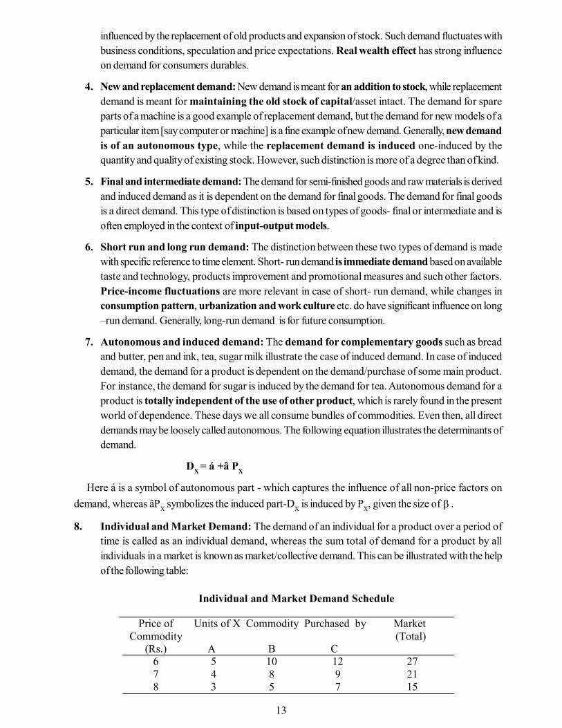
8. Individual and Market Demand: The demand of an individual for a product over a period oftime is called as an individual demand, whereas the sum total of demand for a product by allindividuals in a market is known as market/collective demand. This can be illustrated with the helpof the following table:

Individual and Market Demand Schedule

Price of

Commodity (Rs.)

Units of X Commodity Purchased by Market (Total) A B C

6 5 10 12 27 7 4 8 9 21 8 3 5 7 15

14

The distinction between individual and market demand is very useful for personalized service/targetgroup planning as a part of sales strategy formulation.

9. Total market and segmented market demand: A market for a product may have differentsegments based on location, age, sex, income, nationality etc. The demand for a product in aparticular market segment is called as segmented market demand. Total market demand is asum total of demand in all segments of a market of that particular product. Segmented marketdemand takes care of different patterns of buying behaviour and consumer preferences in differentsegments of the market. Each market segment may differ with respect to delivery prices, net profitmargins, element of competition, seasonal pattern and cyclical sensitivity. When these differencesare glaring, demand analysis is done segment-wise, and accordingly, different marketing strategiesare followed for different segments. For instance, airlines charge different fares from differentpassengers based on their class-economy class and executive/business class.

10. Company and industry demand: A company is a single firm engaged in the production of aparticular product, while an industry is the aggregate / group of firms engaged in the productionof the same product. Thus, the company’s demand is similar to an individual demand, whereas theindustry’s demand is similar to the total demand. For instance, the demand for iron and steel producedby Bokaro plant is an example of company’s demand, but the demand for iron and steel producedby all iron and steel companies including the Bokaro plant is the example of industry demand. Thedeterminants of a company’s demand may be different from industry’s demand. There maybe the inter-company differences with regard to technology, product quality, financial position,market share & leadership and competitiveness. The understanding and knowledge of the relationbetween company and industry demand is of great significance in understanding the different marketstructures/forms based on nature and degree of competition. For example, under perfectcompetition,a firm’s demand curve is parallel to ox-axis, while under monopoly and monopolisticcompetition, it is downward sloping to the right.

2.3 The Law of Demand

The law of demand states an inverse relationship between the price of a commodity and itsquantity demanded, if other things remaining constant (Ceteris Paribus), i.e., at higher price, less quantityis demanded and at lower price, larger quantity is demanded.

Prof. Paul Samuelson has lucidly defined the law of demand. According to him, “if a greaterquantity of a good is thrown on the market then - other things being equal- it can be sold only at a lowerprice.”

Assumptions of the law of demand: The law of demand is based on the following importantceteris paribus assumptions:

• The money income of consumer should remain the same.• There should be no change in the scale of preference (taste, habit & fashion) of the consumer.• There should be no change in the price of substitute goods.• There should be no expectation of price changes of the commodity in near future.• The commodity under question should not be prestigious or of snob appeal.

15

Reasons behind downward sloping demand curves

As we know that most of the demand curves slope downward to the right because of an inverserelationship between the price of a commodity and its quantity demanded. But the question is why inverserelationship exists between the price and quantity demanded. Economists have mentioned the followingreasons of this relationship:

1. Application of the law of diminishing marginal utility: The marginal utility curve slopes downward,hence the demand curve also slopes downward to the right.

2. Substitution effect: The commodity under question becomes cheaper with fall in its price incomparison to its substitutes, therefore demand increases.

3. Income effect: With fall in price of the commodity, demand increases due to increase in realincome as a result of positive income effect.

4. Falling prices attract new consumers as the commodity now becomes affordable to them.

5. With fall in price of the commodity consumers start using it in less important uses, therefore demandincreases. Generally, commodities have different / varied uses.

Exception to the law of demand or upward sloping Demand curve

Sometimes, the law of demand may not hold true, although rarely. In such a situation, a consumermay purchase more at higher price and less at lower price. In this unusual condition, demand curvewill be upward sloping from left to the right as shown below:

D

few real exceptions to the law of Demand

1. Giffen goods: In case of such goods, the income effect is negative and it is stronger than positivesubstitution effect. Examples of such goods are coarse grain like jowar, bajra and coarse cloth.

2. Articles of Distinction/Snob appeal: They satisfy aristocratic desire to preserve exclusivenessfor unique goods- such goods are purchased only by few highly rich people for snob appeal. Forinstance, very costly diamonds, rare paintings, Rolls-Royce- cars and antique items. These goodsare called “veblen goods” after the name of an American economist.

3. Consumers psychological bias or illusion about the quality of commodity with price change.They feel that high priced goods are better quality goods and low price goods are inferior goods.

Positive relationship be tween Px and Dx, hence demand curve is positively sloped. +PP1

+QQ1

X

D

Px

P1

Dx

Y

P

Q Q1 O

16

Prof. Benham has given an example of a book of photographs during the first world war. Thesale of second edition of the book increased tremendously inspite of rise in its price, though thebook contained the same photographs without any change.

4. The law of demand does not apply in case of life saving essential goods and also in times ofextraordinary circumstances like inflation, deflation, war and other natural calamities. The lawalso does not hold true in case of speculative demand. Stock markets are the fine examples ofspeculative demand

2.4 Demand Schedule and Demand Curve

Demand schedule is a statistical/tabular statement showing the different quantities of a commoditywhich will be bought at its different prices during a specified time period. It is a table which representsfunctional relationship between price of a commodity and its quantity demanded. Demand schedule canbe for an individual –known as Individual Demand Schedule (IDS) and it can be for the wholemarket-known as Market Demand Schedule(MDS).MDS can be obtained by aggregating the IDSas illustrated earlier in this unit under the heading of individual and market demand.

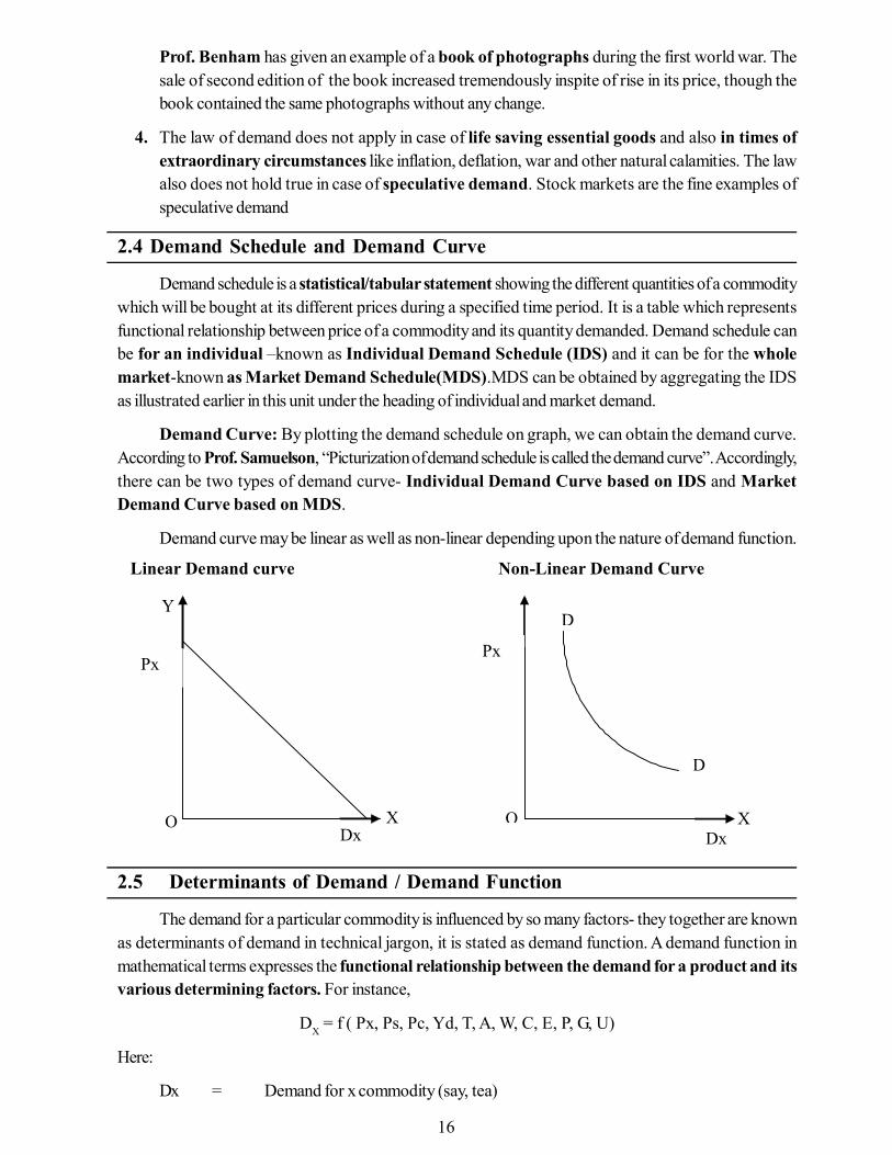
Demand Curve: By plotting the demand schedule on graph, we can obtain the demand curve.According to Prof. Samuelson, “Picturization of demand schedule is called the demand curve”. Accordingly,there can be two types of demand curve- Individual Demand Curve based on IDS and MarketDemand Curve based on MDS.

Demand curve may be linear as well as non-linear depending upon the nature of demand function.

2.5 Determinants of Demand / Demand Function

The demand for a particular commodity is influenced by so many factors- they together are knownas determinants of demand in technical jargon, it is stated as demand function. A demand function inmathematical terms expresses the functional relationship between the demand for a product and itsvarious determining factors. For instance,

DX = f ( Px, Ps, Pc, Yd, T, A, W, C, E, P, G, U)

Here:

Dx = Demand for x commodity (say, tea)

Linear Demand curve Non-Linear Demand Curve

Dx X O

D

O Dx

Y D

Px Px

X

17

Px = Price of x commodity (of tea)Ps = Price of substitute of x commodity (coffee)Pc = Price of complementary goods of x commodity (sugar, milk)Yd = Disposable income of the consumerT = Taste and Preference of the consumerA = Advertisement of x commodityW = Wealth of purchaserC = ClimateE = Price expectation of the consumerP = PopulationG = Govt. policies pertaining to taxes and subsidiesU = Other factors (unspecified/unidentified)

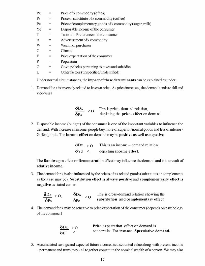
Under normal circumstances, the impact of these determinants can be explained as under:

1. Demand for x is inversely related to its own price. As price increases, the demand tends to fall andvice-versa

δDx

δPx < O This is price- demand relation,

depicting the price- effect on demand

2. Disposable income (budget) of the consumer is one of the important variables to influence thedemand. With increase in income, people buy more of superior/normal goods and less of inferior /Giffen goods. The income effect on demand may be positive as well as negative.

δDx This is an income – demand relation, δYd depicting income effect.

> O <

The Bandwagon effect or Demonstration effect may influence the demand and it is a result ofrelative income.

3. The demand for x is also influenced by the prices of its related goods (substitutes or complementsas the case may be). Substitution effect is always positive and complementarity effect isnegative as stated earlier

4. The demand for x may be sensitive to price expectation of the consumer (depends on psychologyof the consumer)

5. Accumulated savings and expected future income, its discounted value along with present income– permanent and transitory - all together constitute the nominal wealth of a person. We may also

δDx δDx

δPs δPc

> O,

< O This is cross-demand relation showing the substitution and complementary effect

δDx δE

> O <

Price expectation effect on demand is not certain. For instance, Speculative demand.

18

add to his current assets and other forms of physical capital adjusted to price level – This is realwealth and it has influence on the demand. For example, a person has a two wheeler, now maydemand a four wheeler and it can be stated as

6. Taste, preference and habits of consumers may also have decisive influence an the pattern of demand.Social customs, traditions and conventions are Socio – psychological determinants of demand –these are non-economic and non-market factors.

7. Advertisement has great influence on demand. It is in observed fact that sales turnover of firmsincreases up to a point due to advertisement – this is promotional effect on demand and can bestated as

8. Climate also influences the demand for different goods. For instance, the demand for coolers andA.C. increases in summers, while their demand declines in winters.

9. The number and composition (age, sex etc.) of population also influence the demand for goods.

10. Government policy on taxes and subsidies also influences the demand of different goods differently.For instance, increase in tax rates / imposition of new taxes reduce the demand, while increase insubsidies increase the demand.

2.6 Types of Demand

Prof. Baber has mentioned the following three types of demand based on three important factors[price of commodity, income of the consumer and prices of related goods] influencing the demand:

1. Price demand: This type of demand indicates the ‘price effect’, which explains the impact ofchanges in price of a particular product on its quantity demanded, if other factors influencing thedemand remaining constant. The functional relationship between price of a product and its quantitydemanded can be put in the following equation form and be illustrated with price demand schedule:

DX =f[PX]

Here: DX=Demand for x commodity, f= functional relation, and Px = Price of x commodity

Dx δw

> O

δDx δA

> O <

Price Demand Schedule Price of X

Commodity (Px) (Rs.)

Demand for X Commodity (Dx) (units)

Particulars

2 100 3 80 4 40

Inverse relationship between Px and Dx showing negative price effect.

19

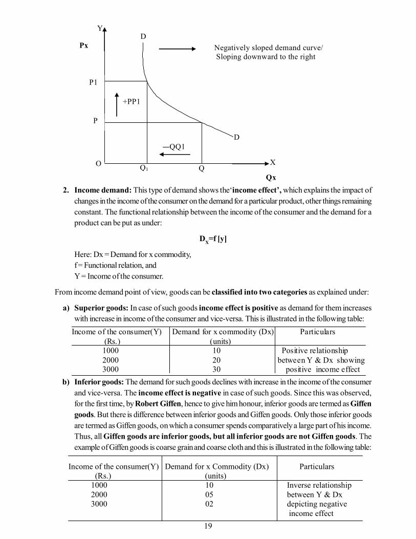
2. Income demand: This type of demand shows the‘income effect’, which explains the impact ofchanges in the income of the consumer on the demand for a particular product, other things remainingconstant. The functional relationship between the income of the consumer and the demand for aproduct can be put as under:

DX=f [y]

Here: Dx = Demand for x commodity,f = Functional relation, andY = Income of the consumer.

From income demand point of view, goods can be classified into two categories as explained under:

a) Superior goods: In case of such goods income effect is positive as demand for them increaseswith increase in income of the consumer and vice-versa. This is illustrated in the following table:

b) Inferior goods: The demand for such goods declines with increase in the income of the consumerand vice-versa. The income effect is negative in case of such goods. Since this was observed,for the first time, by Robert Giffen, hence to give him honour, inferior goods are termed as Giffengoods. But there is difference between inferior goods and Giffen goods. Only those inferior goodsare termed as Giffen goods, on which a consumer spends comparatively a large part of his income.Thus, all Giffen goods are inferior goods, but all inferior goods are not Giffen goods. Theexample of Giffen goods is coarse grain and coarse cloth and this is illustrated in the following table:

Negatively sloped demand curve/

Sloping downward to the right +PP1 QQ1

X

Qx

O

Y

Y

P1

P

Q1 Q

D

D Px

Income of the consumer(Y) Demand for x commodity (Dx) Particulars (Rs.) (units) 1000 10 Positive relationship 2000 20 between Y & Dx showing 3000 30 positive income effect

Income of the consumer(Y) Demand for x Commodity (Dx) Particulars (Rs.) (units) 1000 10 Inverse relationship 2000 05 between Y & Dx 3000 02 depicting negative

income effect Y

20

3. Cross demand: The demand for a commodity is also influenced by the changes in price of itsrelated goods (substitutes or complementary goods as the case may be). This is technically termedas ‘cross effect’ and can be put in the following equation:

DX = f (pr) or DX = f ( py )

Here: DX = Demand for x commodity, f = function, and Pr = Price of related goods,Py = Price of Y commodity- related to x either as substitute or complementary good.

The cross demand of a commodity depends on the nature of its related goods –from this pointof view, it can be of the following two types:

(a) Cross demand for substitutes:Substitute goods / competing goods can easily be used in placeof each other for satisfying a particular want. For example, tea and coffee or pepsi and coca-cola orwheat and rice etc. The impact of changes in price of Y commodity (Py) on the demand for Xcommodity (DX) is called ‘Substitution effect’,which is always positive as illustrated in the followingtable:

Negatively sloped demand curve/

sloping downward to the right +YY1

-QQ1

Y

X

Q Q1

Y1

Y

D

O

D

Dx

Y

Demand curve for superior goods

+yy1 Positively sloped demand

curve/ sloping upward to the right +QQ1

Y1

Dx O

D

Y

D

Q Q1

X

Y

Price of coffee (Py ) Demand for tea (Dx) Particulars (Rs.) (cups) 8 1000 Direct relationship between 9 1200 Py & DX showing positive 10 1800 Substitution effect

21

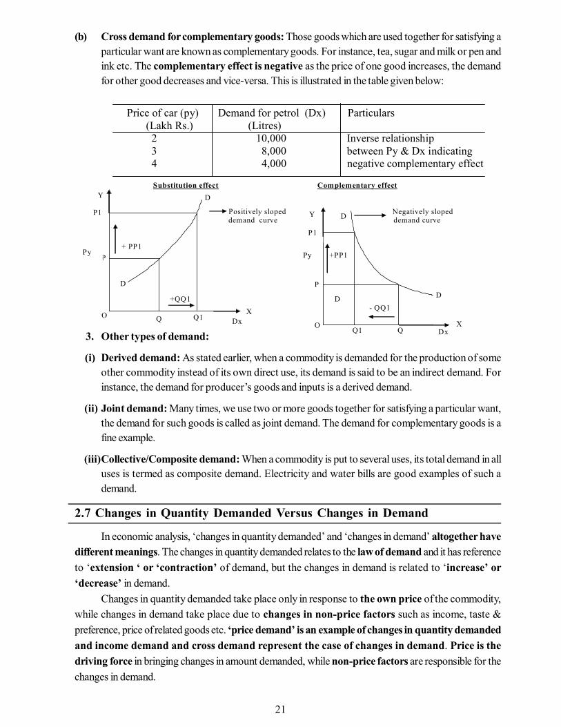
(b) Cross demand for complementary goods: Those goods which are used together for satisfying aparticular want are known as complementary goods. For instance, tea, sugar and milk or pen andink etc. The complementary effect is negative as the price of one good increases, the demandfor other good decreases and vice-versa. This is illustrated in the table given below:

3. Other types of demand:

(i) Derived demand: As stated earlier, when a commodity is demanded for the production of someother commodity instead of its own direct use, its demand is said to be an indirect demand. Forinstance, the demand for producer’s goods and inputs is a derived demand.

(ii) Joint demand: Many times, we use two or more goods together for satisfying a particular want,the demand for such goods is called as joint demand. The demand for complementary goods is afine example.

(iii)Collective/Composite demand: When a commodity is put to several uses, its total demand in alluses is termed as composite demand. Electricity and water bills are good examples of such ademand.

2.7 Changes in Quantity Demanded Versus Changes in Demand

In economic analysis, ‘changes in quantity demanded’ and ‘changes in demand’ altogether havedifferent meanings. The changes in quantity demanded relates to the law of demand and it has referenceto ‘extension ‘ or ‘contraction’ of demand, but the changes in demand is related to ‘increase’ or‘decrease’ in demand.

Changes in quantity demanded take place only in response to the own price of the commodity,while changes in demand take place due to changes in non-price factors such as income, taste &preference, price of related goods etc. ‘price demand’ is an example of changes in quantity demandedand income demand and cross demand represent the case of changes in demand. Price is thedriving force in bringing changes in amount demanded, while non-price factors are responsible for thechanges in demand.

Price of car (py) Demand for petrol (Dx) Particulars (Lakh Rs.) (Litres) 2 10,000 Inverse relationship 3 8,000 between Py & Dx indicating 4 4,000 negative complementary effect

Substitution effect Complementary effect Positively sloped Negatively sloped demand curve demand curve

+ PP1 +PP1

+QQ1 - QQ1

P1

Py

D

Dx X

P

P

D

Y

O

X Q O

Y

Q1

P1

D

Q Q1 Dx

D

D

Py

22

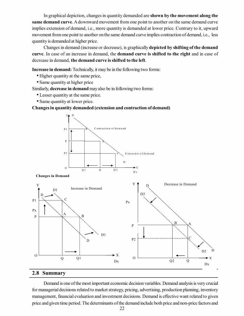
In graphical depiction, changes in quantity demanded are shown by the movement along thesame demand curve. A downward movement from one point to another on the same demand curveimplies extension of demand, i.e., more quantity is demanded at lower price. Contrary to it, upwardmovement from one point to another on the same demand curve implies contraction of demand, i.e., lessquantity is demanded at higher price.

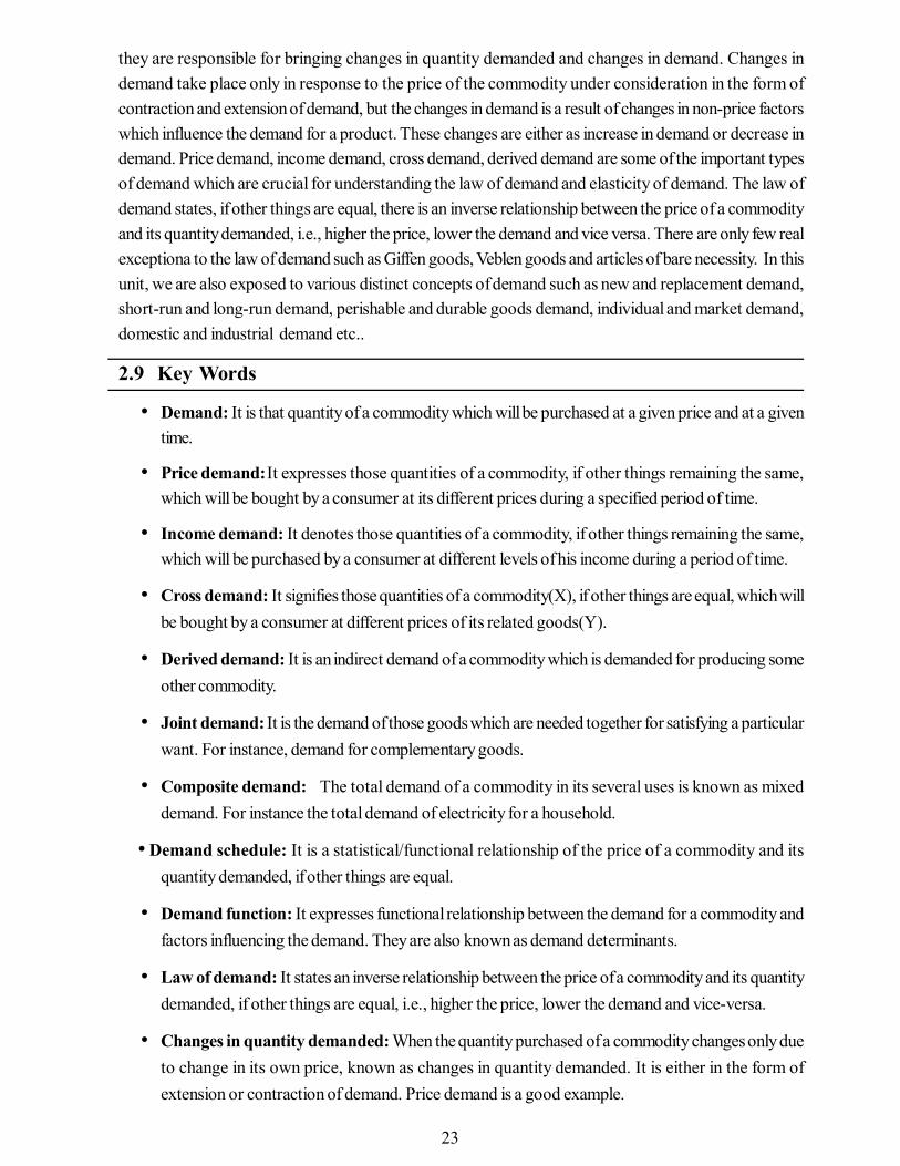
Changes in demand (increase or decrease), is graphically depicted by shifting of the demandcurve. In case of an increase in demand, the demand curve is shifted to the right and in case ofdecrease in demand, the demand curve is shifted to the left.

Increase in demand: Technically, it may be in the following two forms: • Higher quantity at the same price, • Same quantity at higher priceSimilarly, decrease in demand may also be in following two forms: • Lesser quantity at the same price. • Same quantity at lower price.Changes in quantity demanded (extension and contraction of demand)

2.8 Summary

Demand is one of the most important economic decision variables. Demand analysis is very crucialfor managerial decisions related to market strategy, pricing, advertising, production planning, inventorymanagement, financial evaluation and investment decisions. Demand is effective want related to givenprice and given time period. The determinants of the demand include both price and non-price factors and

D

C

Y D

O

P

X Q 2 Q Q 1

P 2

P 1

A

B

D x

C o ntr act io n o f d e m a nd

E xte n s io n o f d e m a nd

Changes in Demand Decrease in Demand Increase in Demand

Y

X

A

D

A B

C

D2

Y

D

Px

D1

D D1

B

C

P2

O O

Px

Q2 Q

P1

P

X Q1 Q

D

D2

P

Dx Dx

23

they are responsible for bringing changes in quantity demanded and changes in demand. Changes indemand take place only in response to the price of the commodity under consideration in the form ofcontraction and extension of demand, but the changes in demand is a result of changes in non-price factorswhich influence the demand for a product. These changes are either as increase in demand or decrease indemand. Price demand, income demand, cross demand, derived demand are some of the important typesof demand which are crucial for understanding the law of demand and elasticity of demand. The law ofdemand states, if other things are equal, there is an inverse relationship between the price of a commodityand its quantity demanded, i.e., higher the price, lower the demand and vice versa. There are only few realexceptiona to the law of demand such as Giffen goods, Veblen goods and articles of bare necessity. In thisunit, we are also exposed to various distinct concepts of demand such as new and replacement demand,short-run and long-run demand, perishable and durable goods demand, individual and market demand,domestic and industrial demand etc..

2.9 Key Words

• Demand: It is that quantity of a commodity which will be purchased at a given price and at a giventime.

• Price demand:It expresses those quantities of a commodity, if other things remaining the same,which will be bought by a consumer at its different prices during a specified period of time.

• Income demand: It denotes those quantities of a commodity, if other things remaining the same,which will be purchased by a consumer at different levels of his income during a period of time.

• Cross demand: It signifies those quantities of a commodity(X), if other things are equal, which willbe bought by a consumer at different prices of its related goods(Y).

• Derived demand: It is an indirect demand of a commodity which is demanded for producing someother commodity.

• Joint demand: It is the demand of those goods which are needed together for satisfying a particularwant. For instance, demand for complementary goods.

• Composite demand: The total demand of a commodity in its several uses is known as mixeddemand. For instance the total demand of electricity for a household.

• Demand schedule: It is a statistical/functional relationship of the price of a commodity and itsquantity demanded, if other things are equal.

• Demand function: It expresses functional relationship between the demand for a commodity andfactors influencing the demand. They are also known as demand determinants.

• Law of demand: It states an inverse relationship between the price of a commodity and its quantitydemanded, if other things are equal, i.e., higher the price, lower the demand and vice-versa.

• Changes in quantity demanded: When the quantity purchased of a commodity changes only dueto change in its own price, known as changes in quantity demanded. It is either in the form ofextension or contraction of demand. Price demand is a good example.

24

• Changes in demand: When quantity bought changes due to changes in other determinants ofdemand except the price of the commodity under consideration, it is termed as changes in demand.It can be either increase or decrease in demand. Income demand and cross demand are goodexamples.

• Price effect: It is the influence of changes in price of a commodity on its quantity demanded. It isgenerally negative.

• Income effect: It signifies the impact of changes in income of the consumer on the demand for acommodity. It can be positive or negative.

• Cross effect: It expresses the impact of changes in price of related goods (Py) on the demand ofthe parent product.(Dx) It can also be positive or negative.

• Substitute goods: Those goods which can easily be used in place of each other for satisfying aparticular want. For instance, tea and coffee.

• Complementary goods: Those goods which are required together for satisfying a particular want.For instance, tea, sugar& milk or cricket bat and ball.

• Superior/normal goods: These are the goods the demand for which increases with increase inincome of the consumer and vice-versa.

• Giffen/inferior goods:Those goods whose demand declines with increase in income of theconsumers. For instance, Coarse grain and clothes.

• Veblen Effect : It refers to the desire of a person (usually very rich) to own exclusive or uniqueproduct – called veblen good / snob good. It serves as prestige symbol.

• Bandwagon Effect : It is also known as demonstration effect : The demand for a product seemsto be determined basically not by the utility of it, but mostly on account of consumption of trendsetters such as cricket /film stars, models, neighbours etc.

• Ceteris Paribus : It means other things being equal. It is a French word


1. Make a list of factors which may determine the demand for

(a) a consumer durable item like car / washing machine(b) an intermediate good like cables(c) a producer good like machinery / equipment

Analyse the common factors.

2. Draw the following :(a) Exceptional Demand Curve(b) Income Demand Curve for Superior goods(c) Income Demand Curve for Giffin goods

25

(d) Cross demand curve for Substitute goods(e) Cross demand curve for complementary goods

3. Distinguish between the following :(a) Extension of demand and increase in demand(b) Contraction of demand and decrease in demand(c) Want and demand(d) Substitution effect and income effect(e) Inferior goods and Giffen goods(f) Direct and derived demand

4. Construct a typical individual and market demand schedule and draw the demand curve based onthem

2.11 Suggested Books / References

1. Mithani D.M. : Managerial Economics, Himalaya Publishing House, Mumbai

2. Dwivedi, D.N. : Managerial Economics, Vikas Publishing House Pvt. Ltd, New Delhi

3. Misra & Puri : Economics for Managers, Himalaya Publishing House, Mumbai

4. Adhikary M. : Managerial Economics, Khosla Educational Publishers, Delhi

5. Mote, Paul & Gupta : Managerial Economics – Concepts & Cases, Tata Mc-Graw Hill PublishingCompany Ltd., Mumbai

6. Koutsoyiannis, A : Modern Microeconomics, The Macmillan Press Ltd.,, London

26

Unit - 3 Elasticity of Demand and Demand EstimatesUnit-structure

3.0 Objectives3.1 Introduction3.2 Concept of Demand3.3 Concept of Elasticity of Demand3.4 Types of Elasticity of Demand3.5 Degree of Price Elasticity of Demand3.6 Income Elasticity of Demand3.7 Cross Elasticity of Demand3.8 Measuring the Price Elasticity of Demand3.9 Factors Influencing Elasticity of Demand3.10 Importance of Elasticity of Demand3.11 Summary3.12 Self Assessment Test3.13 Suggested Books / References

3.0 Objectives

After studying this unit you should be able to understand:

• The concept of elasticity of Demand• Types and degree of elasticity and price elasticity of Demand• Methods of measuring the elasticity of Demand – Flux’s percentage method, Total outlay method, ARC method and point elasticity of demand method.

3.1 Introduction

Demand and supply play an important role in economics as well as in an economy. Therefore thisone is a famous saying that if a parrot is taught demand & supply, demand & supply in the answers of thequestions it may prove to be a good economist. This proves that demand & supply play a prominent rolein the entire economics. With this background, before we discuss the elasticity of demand, it is better thatwe should know a brief concept of demand. Law of demand only describes direction of change in demandbut elasticity of demand describes degree of change in demand.

3.2 Concept of Demand

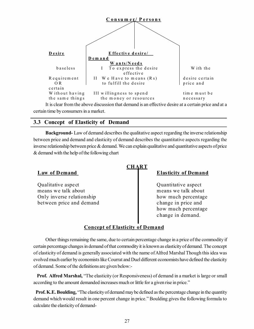
Generally demand is that commodity which is demanded by the consumer at a certain price and ata time. In a practical life a person uses so many words instead of demand for example- desire, effectivedesire, wants, needs etc. but in a practical market, the concept is different. We can explain with the help

of following chart-

27

It is clear from the above discussion that demand is an effective desire at a certain price and at acertain time by consumers in a market.

3.3 Concept of Elasticity of Demand

Background- Law of demand describes the qualitative aspect regarding the inverse relationshipbetween price and demand and elasticity of demand describes the quantitative aspects regarding theinverse relationship between price & demand. We can explain qualitative and quantitative aspects of price& demand with the help of the following chart

Other things remaining the same, due to certain percentage change in a price of the commodity ifcertain percentage changes in demand of that commodity it is known as elasticity of demand. The conceptof elasticity of demand is generally associated with the name of Alfred Marshal Though this idea wasevolved much earlier by economists like Courrat and Duel different economists have defined the elasticityof demand. Some of the definitions are given below:-

Prof. Alfred Marshal, “The elasticity (or Responsiveness) of demand in a market is large or smallaccording to the amount demanded increases much or little for a given rise in price.”

Prof. K.E. Boulding, “The elasticity of demand may be defined as the percentage change in the quantitydemand which would result in one percent change in price.” Boulding gives the following formula tocalculate the elasticity of demand-

C o n s u m e r / P e r s o n s D e s ir e E ff e c tiv e d e s ir e / D e m a n d W a n ts /N e e d s

b a se le s s I T o e x p re ss th e d e s ir e W ith th e e ff e c t iv e

R e q u i re m e n t I I W e H a v e to m e a n s (R s ) d e s i re c e r ta in O R to f u lf i l l th e d e s ire p r ic e a n d c e r ta in W i th o u t h a v in g I I I w ill in g n e ss to sp e n d t im e m u s t b e th e s a m e th in g s th e m o n e y o r r e s o u rc e s n e c e s sa ry

CHART Law of Demand Elasticity of Demand Qualitative aspect Quantitative aspect means we talk about means we talk about Only inverse relationship how much percentage between price and demand change in price and how much percentage change in demand.

Concept of Elasticity of Demand

28

Elasticity of Demand

Mrs. John Robinson, “The elasticity of demand at any price or at any output is equal to the proportionalchange of amount demanded in response to a small change in price divided by the proportional change inprice.”

Robinson also gives the following formula for calculation of the elasticity of demand.

Elasticity of Demand

3.4 Types of Elasticity of Demand

Before we discuss the types and degree of elasticity of demand it is better if we can express entirestructure of types & degree of elasticity of demand with the help of the following chart-

Price Elasticity of Demand (EP)- Other things remaining the same due to certain percentage change inprice if certain percentage change in demand of commodity is there, it is known as price elasticity ofdemand. It is measured as percentage change in quantity demanded divided by the percentage change inprice.

T y p e s o f E l a s t i c i t y o f D e m a n d

[ A ] P r i c e E l a s t i c i t y [ B ] I n c o m e E l a s t i c i t y [ C ] C r o s s E l a s t i c i t y o f D e m a n d o f D e m a n d o f D e m a n d [ E P ] [ E Y ] [ E C ]

I P o s i t i v e I I N e g a - I P e r f e c t E l a s t i c i t y I I H i g h E l a s t i c i t y I I I U n i t E l a s t i c i t y t i v e o f D e m a n d o f D e m a n d o f D e m a n d [ E C ] [ E C ] [ E P = α ] [ E P > 1 ] [ E P = 1 ]

I V H i g h I n E l a s t i c i t y V P e r f e c t O f D e m a n d I n E l a s t i c i t y o f D e m a n d [ E P < 1 ] [ E P = 0 ] I P o s i t i v e I I N e g a t i v e I I I Z e ro E Y E Y E Y

commodity theof price ain change Percentagedemandin change Percentage

fdfffdfdfdf

commodity theof price ain change Percentagedemandin change Percentage

Or % Q

% P %ΔΔ%ΔΔ

orpriceinchangePercentage

demandedQuantityinchangePercentageED

29

Where Ep = Price Elasticity P = Price Q = Quantity

= Change

3.5 Degree of Price Elasticity of Demand

I Perfectly Elastic Demand (Ep=á):

When minor, nothing or as good as zero percentage change in price results in tremendous percentagechange in demand, it is known as perfectly elastic demand. We can say in other words that it is a situationin which demand of a commodity continuously changes without any change in price. It can be explainedwith the help of following example and diagram.

Example:-

II Highly Elastic Demand (e>1):

When less percentage change in price of commodity and if as compared to that more percentagechange in demand is there, it is known as highly elastic demand. We can say in other words that it refers toa situation in which percentage change in demand of commodity is higher than percentage change in priceof that commodity. We can explain this with the help of the following example and diagram-

III Unitary Elastic Demand (e=1)

When equal percentage or a proportionate change in price of commodity and demand of commodityis there, it is known as unitary elastic demand . It means that percentage change in demand of a commodityis equal to percentage change in price. We can explain this with the help of following example and diagram-

Y 0.25 or 0.10 % Change e=α D In price Price p 10 % or 15 % Change in demand

0 X Demand

E x am ple :- Y D 5% C hang e In p rice P 1 P rice p e> 1 20% C hange in dem and D

0 X Q 1 Q 2

D em and

E x a m ple :- Y D 1 0 % C h a n ge In p ric e P 1 e = 1 P rice p 1 0 % C h a ng e in dem a n d D

0 X Q Q 1

D e m a nd

30

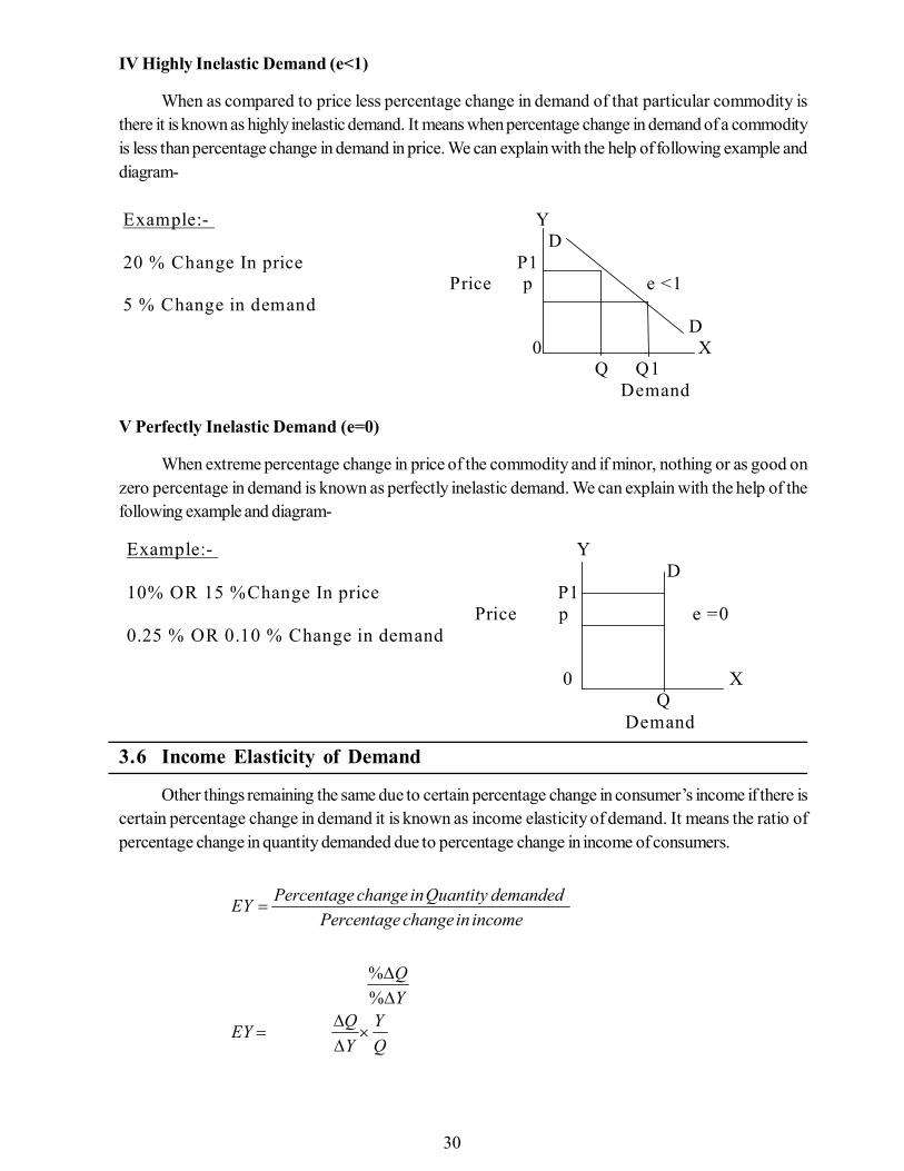
IV Highly Inelastic Demand (e<1)

When as compared to price less percentage change in demand of that particular commodity isthere it is known as highly inelastic demand. It means when percentage change in demand of a commodityis less than percentage change in demand in price. We can explain with the help of following example anddiagram-

V Perfectly Inelastic Demand (e=0)

When extreme percentage change in price of the commodity and if minor, nothing or as good onzero percentage in demand is known as perfectly inelastic demand. We can explain with the help of thefollowing example and diagram-

3.6 Income Elasticity of Demand

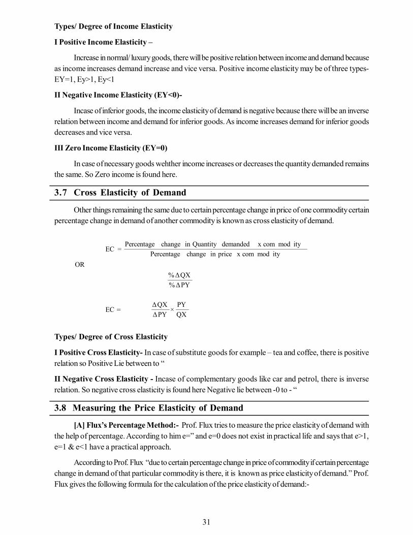
Other things remaining the same due to certain percentage change in consumer’s income if there iscertain percentage change in demand it is known as income elasticity of demand. It means the ratio ofpercentage change in quantity demanded due to percentage change in income of consumers.

QY

YQEY

YQ

incomeinchangePercentagedemandedQuantityinchangePercentageEY

%%

Example:- Y D 20 % Change In price P1 Price p e <1 5 % Change in demand D 0 X Q Q1

Demand

Example:- Y D 10% OR 15 %Change In price P1 Price p e =0 0.25 % OR 0.10 % Change in demand 0 X

Q Demand

31

Types/ Degree of Income Elasticity

I Positive Income Elasticity –

Increase in normal/ luxury goods, there will be positive relation between income and demand becauseas income increases demand increase and vice versa. Positive income elasticity may be of three types-EY=1, Ey>1, Ey<1

II Negative Income Elasticity (EY<0)-

Incase of inferior goods, the income elasticity of demand is negative because there will be an inverserelation between income and demand for inferior goods. As income increases demand for inferior goodsdecreases and vice versa.

III Zero Income Elasticity (EY=0)

In case of necessary goods wehther income increases or decreases the quantity demanded remainsthe same. So Zero income is found here.

3.7 Cross Elasticity of Demand

Other things remaining the same due to certain percentage change in price of one commodity certainpercentage change in demand of another commodity is known as cross elasticity of demand.

QXPY

×PYΔQXΔ

=EC

PYΔ%QXΔ%

ORitymodcomxpriceinchangePercentage

itymodcomxdemandedQuantityinchangePercentage=EC

Types/ Degree of Cross Elasticity

I Positive Cross Elasticity- In case of substitute goods for example – tea and coffee, there is positiverelation so Positive Lie between to “

II Negative Cross Elasticity - Incase of complementary goods like car and petrol, there is inverserelation. So negative cross elasticity is found here Negative lie between -0 to - “

3.8 Measuring the Price Elasticity of Demand

[A] Flux’s Percentage Method:- Prof. Flux tries to measure the price elasticity of demand withthe help of percentage. According to him e=” and e=0 does not exist in practical life and says that e>1,e=1 & e<1 have a practical approach.

According to Prof. Flux “due to certain percentage change in price of commodity if certain percentagechange in demand of that particular commodity is there, it is known as price elasticity of demand.” Prof.Flux gives the following formula for the calculation of the price elasticity of demand:-

32

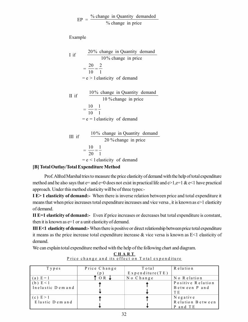
[B] Total Outlay/Total Expenditure Method

Prof. Alfred Marshal tries to measure the price elasticity of demand with the help of total expendituremethod and he also says that e= and e=0 does not exist in practical life and e>1,e=1 & e<1 have practicalapproach. Under this method elasticity will be of three types:-I E> 1 elasticity of demand:- When there is inverse relation between price and total expenditure itmeans that when price increases total expenditure increases and vice versa , it is known as e>1 elasticityof demand.II E=1 elasticity of demand:- Even if price increases or decreases but total expenditure is constant,then it is known as e=1 or a unit elasticity of demand.III E<1 elasticity of demand:- When there is positive or direct relationship between price total expenditureit means as the price increase total expenditure increase & vice versa is known as E<1 elasticity ofdemand.We can explain total expenditure method with the help of the following chart and diagram.

demandofelasticity1<e=11

=2010

=

priceinchange%20demandQuantityinchange%10

ifIII

demandofelasticity1=e=11

=1010

=


ifII

demandofelasticity1>e=12

=1020

=


ifI

Example

priceinchange%demandedQuantityinchange%

=EP

C H A R T P r i c e c h a n g e a n d i t s e f f e c t o n T o ta l e x p e n d i tu r e

T y p e s P r i c e C h a n g e

( p ) T o ta l

E x p e n d i tu r e ( T E ) R e la t i o n

( a ) E = 1 O R N o C h a n g e N o R e la t i o n ( b ) E < 1 I n e l a s t i c D e m a n d

P o s i t i v e R e l a t i o n B e tw e e n P a n d T E

( c ) E > 1 E l a s t i c D e m a n d

N e g a t iv e R e l a t i o n B e tw e e n P a n d T E

33

[C] ARC Elasticity of Demand:-

When we measure any two particular points of the demand curve, it is known as ARC elasticity ofdemand. When there is a major percentage change in price or in a demand then ARC elasticity of demandmethod is appropriate for the economist.

In reality we may come across demand schedules which have gaps in prices as well as in quantities.ARC signifies a segment or portion of a curve between two points. The formula for measuring the ARCelasticity is :-

Original quantity- New quantityOriginal quantity+New quantity

Ec= Original price – New PriceOriginal Price+ New Price

1

1

1

1

1

1

1

1

1

1

1

1

QQP+P

÷P+PQQ

=

PPP+P

×Q+QQQ

=

P+PPP

÷Q+QQQ

=

In Which – Q = Original quantity demandedQ1 = New quantity demandedP = Original PriceP1 = New Price

Let us take a concrete example to explain the arc method. The demand when the price was 3000units per week and the price was Rs. 2/- per unit. The demand contracted to 2700 units when price wasraised to Rs. 2.10 per unit. Calculate elasticity of demand by ARC method. The formula is:-

1

1

1

1

1

1

1

1

PPP+P

×Q+QQQ

=

P+PPP

÷Q+QQQ

=Ec

Y D

P5 e>1 Inverse relationship between price and P4 Total Expenditure

P3

Price e=1 Price Increase or Decrease Total P2 Expenditure is constant P1 e<1 Direct or positive relationship between P price and Total Expenditure D 0 X Total Expenditure

34

Now substituting with the figures given in the question we have

)OmittedbeMayymbolMinusS(16.2=1941

=

10410

×5700300

=

210200210+200

×2700+300027003000

=Ec

Elasticity of demand is 2.16

[D] Point Elasticity of Demand:-

When there is minor percentage change in price & demand then point elasticity of demand methodis useful for the economist. Price elasticity of demand can also be measured with the help of what is knownas the “Point Method.” According to this method , elasticity of demand on each point of a demand curveshall be different, and can be measured with the help of the following formula:-

Point elasticity of demand curvedemandofsegmentUppercurve demand theof Sagment Lower

=

Elasticity at different point of a straight line demand curve by different points use the above formula.We can calculate the elasticity of demand and at any point on a straight line demand curve—

Y D P 1 A P r ic e P A R C E la s tic i ty P B Q D 0 Q Q 1 X D e m a n d

Y A e=? It shall be Zero at the point P1 e>1 where the demand curve Price Touches horizontal axis; and it P e=1 shall be infinity where it Touched vertical axis. It shall

P2 e<1 be equal to unity at the central Point of the demand curve.

0 e=0 X B

35

It shall be less than unity in the lower segment and more than unity in the upper segment of the curve.It is equal to unity at the middle point of the curve AB less than unity in the lower segment and more thanunity in the upper segment.

It is clear from the above diagram that AB is the straight line demand curve. Let us take price P as themiddle point of the demand curve AB.

Now, E at point

1=PAPB

=P To illustrate the same point

(For PB= PA)

Let us assume AB to represent 6 cm. then the middle point of AB, PB will be equal to 3cm and PA will beequal to 3 cm.

E at point 1=cm3cm3

=PAPB

=P

Let us take a price p1 at the point higher than the middle point of the demand curve AB.

E at point =APBP

=P1

11 More than 1 (P1B>P1A)

Using the numerical example of AB being equal to 6cm; then

E at point cm2cm4

=APBP

=P1

11 = 2 more than 1

At a price lower than the middle point of the demand curve (P2) elasticity will be less unity as farinstance.

E at point =BPBP

=P1

22 Less than 1 (P2B<P2A)

If P2 B is 2 c, and P2A is 4cm ; than

E at point cm4cm2

=APBP

=P2

22 0.5 Less than 1.

3.9 Factors Influencing Elasticity of Demand

Demand is a function of price, income, taste, hobby, nature of consumer population, govt. policyetc. Elasticity of demand tends to be different for different types of goods it will differ from market tomarket with this background we can explain the factors influencing elasticity of demand.

1. Nature of commodity - These who have no substitute goods will have an inelasticity of demand.The consumers will buy almost a fixed demand whether the price is higher or lower. Demand forluxuries, on the other hand, is elastic in nature.

36

2. Different uses of the commodity- A commodity that has several kinds of uses is apt to be elasticin demand. For each single use demand may be inelastic so that when price of the commodity goesdown only a little more is purchased for every use.

3. Availability of substitute goods- When there exists a class substitute in the relevant price range,its demand will tend to be elastic. But in respect of commodities having no substitutes, theirdemand will be the same inelastic.

4. Consumer’s income - Generally larger the income, the overall demand for commodities tends tobe relatively inelastic. The redistribution of income in favour of low income people may tend tomake demand for some goods relatively inelastic.

5. Proportion of expenditure- Items that constitute a smaller amount of expenditure in a consumer’sfamily budget tend to have a relatively inelastic demand, e.g., a cinegoer who sees a film every fortnight is not likely to give it up when the ticket rates are raised. But one who sees a film everyalternate day perhaps may cut down his number of films. So is the case with matches, sugar etc.

6. Durability of the commodity- In the case of durable goods, the demand generally tends to beinelastic in the short run, e.g., furniture. bicycle radio, etc. In the perishable commodities, on theother hand, demand is relatively elastic, e.g., milk , vegetables, etc.

7. Influence of habit and customs- There are certain articles which have a demand on account ofconventions, customs or habit and in these cases, elasticity is less, e.g., Mangal Sutra to a Hindubride or cigarettes to a smoker have inelasticity of demand.

8. Complementary goods- Goods which are jointly demanded have less elasticity, e.g., ink, petrolhave inelastic demand for this reason.

9. Recurrence of demand- If the demand for a commodity is of a recurring nature, its price elasticityis higher than that of a commodity which is purchased only once. For instance, bicycle, tape recorders,radios, etc. are purchased only once, hence their price elasticity will be less. But the demand forcassettes or tape spools would be more price elastic.

10. Possibility of postponement- When the demand for a product is postponable, it will tend to beprice elastic. In the case of consumption goods which are urgently and immediately required, theirdemand will be inelastic.

3.10 Importance of Elasticity of Demand

The concept of elasticity of demand is of considerable significance in various situations, which weshall briefly summaries below: 1. Helpful to a monopolist in fixing price- The individual producer under imperfect competition has

to consider the demand for his product when he fixes its price. He has to take into account theresponse of his customers in formulating his price policy. Like wise the monopolist has to study theelasticity of demand of his product before he fixes its price.

2. Helpful to the Government in formulating Taxation Policies- The concept of elasticity ofdemand also proves helpful to the Government in the formulation of its economic and taxationpolicies, The finance minister has to consider the nature of the elasticity of demand for a commoditybefore levying an excise tax on it.

3. Helpful in Determination of rewards for factors of Production- The concept of elasticity ofdemand also influences the determination of the rewards for factors of production in a privateenterprise economy. If the demand for labour on a particular industry is relatively inelastic, it will beeasier for the trade union to get their wages raised. The same remarks apply to other factors ofproduction whose demands are relatively inelastic.

37

4. Helpful in determination of terms of trade- It is possible to calculate the terms of trade betweentwo countries only by taking into account the mutual elasticities of demand for each others products.The term “Terms of Trade” implies the rate at which one unit of a domestic commodity will exchangefor units of commodity of a foreign country.

5. Helpful in determining the Rate of Exchange- The concept of elasticity of demand also helpsthe government in fixing an appropriate foreign rate of exchange for its domestic currency in relationto the currencies of other countries. Before deciding to devalue or revalue domestic currency inrelation to foreign currencies the government has to study carefully the elasticites of demand for itsimports and exports.

6. Helpful in declaring certain industries as ‘Public Utilities’- The concept of elasticity of demandalso enables the government to decide as to what particular industries should be declared as publicutilities and being consequently owned and operated by state.

3.11 Summary

Demand & law of demand is related with the Qualitative aspect regarding the inverse relationshipbetween price & demand and elasticity of demand is related with the Quantitative aspect regarding theinverse relationship between price and demand. Elasticity of demand means due to certain percentagechange in price if certain percentages change in Quantity demand by consumers.

Price elasticity of demand is a measure of the extent to which quantity demanded of a good respondsto a change in its price. When the numerical measure is less then one, we say that the demand is inelastic.When it is e>1, we say demand is elastic and when it is e=1 we say demand is unitary Two special casesare when elasticity equals zero (e=0) or infinity (e=”). When elasticity is (e=0), the quantity demandeddoes not change at all as price changes, and when elasticity e=”, a very small reduction in price increasesthe quantity demanded from zero to an infinity large number.

Price elasticity can be measured at a point or between two points Here we use the concepts ofpoint elasticity and ARC elasticity respectively. The main determinants of elasticity are the availability ofsubstitutes for the commodity, numbers of uses of the commodity, nature of commodity etc.


1. What do you mean by elasticity of demand? Explain various types of demand elasticity withillustrations.

2. What are the various factors affecting price elasticity of demand?3. Discuss the various methods of measuring the elasticity of demand.4. Write a short note on the following points :-

A. Total Expenditure MethodB. ARC elasticity of demand Method.

5. Discuss the degree of price elasticity of demand with the help of example and diagram.

3.13 Suggested Books/References

1. Dwivedi, D.N. : Managerial Economics, Himalaya Publishing House, Mumbai.

2. Mate, Paul & Gupta : Managerial Economics-concept & cases tala Mc Grow Hill publicationcompany limited, Mumbai

38

Unit - 4 Demand ForecastingUnit Structure

4.0 Objectives4.1 Introduction4.2 Concept of Demand Forecasting4.3 Features of Demand Forecasting4.4 Importance of Demand Forecasting4.5 Scope of Demand Forecasting4.6 Methods of Demand Forecasting4.7 Demand Forecasting Process4.8 Summary4.9 Self Assessment Test4.10 Suggested Books / References

4.0 Objectives

Under dynamic business conditions demand forecasting is very difficult. It is also difficult in case ofnew products about which no information is available about consumer’s preferences. In this chapter. weshall discuss the purpose of demand forecasting, scope, steps and methods of demand forecasting.

4.1 Introduction

Generally, there is uncertainity in over every decision-making process. The producer of somegoods or any other decision-making authority or the government must keep in view the existing level ofdemand for the product in question and estimate the prevalent gap between demand and supply. Thedecision maker, whether a firm or a state planning agency, must not only estimate the present level ofdemand but also forecast the demand for a future date.

Degree of risk depends upon the nature of business. All the risks can not be completely eradicatedbut by proper planning these risks can be minimized. Demand forecasting is also one of the techniques tominimize the risk and uncertainity.

4.2 Concept of Demand Forecasting

Forecasting of demand is the art of predicting demand for a product or a service at some future dateon the basis of certain present and past behaviour patterns of some related events. Please remember thatforecasting is no simple guessing but it refers to estimating scientifically and objectively on the basis ofcertain facts and events relevant to the art of forecasting.

Cundif and Still:- “ According to Cundif and Still sales forecasting is an estimate of sales during aspecified future period on which estimates is tied to a proposed marketing plan which assumes a particularset of uncontrollable and competitive forces.”

According to Philip Kotler:- “ The Company sales forecast is the expected level of company salesbased on a chosen marketing plan and assumed marketing environment.”

39

4.3 Features of Demand Forecasting

From the above discussions the following features of demand forecasting emerge:

1. Demand forecasting is based on past data and present positions.

2. Demand forecasting may be monetary or physical.

3. Demand forecasting gives basis to future planning.

4. Demand forecasting is made for a certain period.

5. Future sales and profit estimate can be made by demand forecasting.

4.4 Importance of Demand Forecasting

Demand forecasting is important for every producer. He has to know the present level of demandas also the increase that is expected to take place in the demand for his product over time. Demandforecasts are generally useful for the following categories of decision makers:-

1. Importance for the producers. 2. Importance for policy makers and planners. 3. Importance for estimating financial requirements. 4. Utility for determination of sales target & incentive. 5. Importance for regular supply of labour and raw material is made possible by demand forecasting. 6. Production planning is possible with the help of demand forecasting. 7. Use for other groups of the society researchers, social workers and other who have a futuristic

approach.

4.5 Scope of Demand Forecasting

Demand forecasting can be at the international level depending upon the area of operation of giveneconomic institution. It can also be confined to a given product or service supplied by a small firm in localarea. The scope of work will depend upon the area of operation in the present and proposed in futuremuch would depend upon the cost and time involved in relation to the benefit of the information acquiredthrough the study of demand. The factors determining the scope of demand forecasting are as follows:-

1. Period conversed under demand forecasting. 2. Levels of demand forecasting. 3. Purpose of demand forecasting. 4. Nature of product. 5. Miscellaneous factors- socio-psychological factors, degree of competition impact of risk and

uncertainity.

4.6 Methods of Demand Forecasting

Demand forecasting is a very absorbing and difficult exercise. Consumer’s behaviour is the mostunpredictable thing in the world because it is motivated and influenced by multiplicity. Moreover; economistand statisticians over the years have developed several methods of demand forecasting. Each of thesemethods has its relative merits and demerits. Selection of the right method is essential to make demandforecasting accurate and credible. The methods of demand forecasting can be summarized in the form ofa chart as follows:-

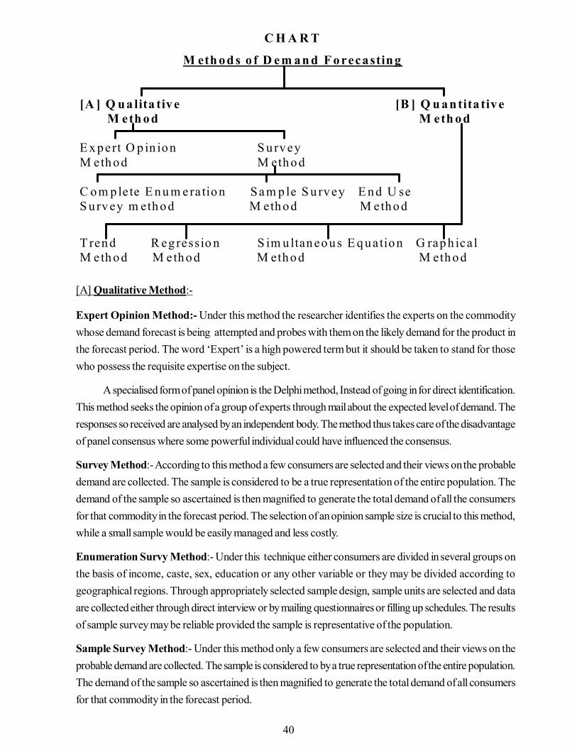
40

[A] Qualitative Method:-

Expert Opinion Method:- Under this method the researcher identifies the experts on the commoditywhose demand forecast is being attempted and probes with them on the likely demand for the product inthe forecast period. The word ‘Expert’ is a high powered term but it should be taken to stand for thosewho possess the requisite expertise on the subject.

A specialised form of panel opinion is the Delphi method, Instead of going in for direct identification.This method seeks the opinion of a group of experts through mail about the expected level of demand. Theresponses so received are analysed by an independent body. The method thus takes care of the disadvantageof panel consensus where some powerful individual could have influenced the consensus.

Survey Method:- According to this method a few consumers are selected and their views on the probabledemand are collected. The sample is considered to be a true representation of the entire population. Thedemand of the sample so ascertained is then magnified to generate the total demand of all the consumersfor that commodity in the forecast period. The selection of an opinion sample size is crucial to this method,while a small sample would be easily managed and less costly.

Enumeration Survy Method:- Under this technique either consumers are divided in several groups onthe basis of income, caste, sex, education or any other variable or they may be divided according togeographical regions. Through appropriately selected sample design, sample units are selected and dataare collected either through direct interview or by mailing questionnaires or filling up schedules. The resultsof sample survey may be reliable provided the sample is representative of the population.

Sample Survey Method:- Under this method only a few consumers are selected and their views on theprobable demand are collected. The sample is considered to by a true representation of the entire population.The demand of the sample so ascertained is then magnified to generate the total demand of all consumersfor that commodity in the forecast period.

C H A R T

M eth o d s o f D e m a n d F o reca sting

[A ] Q ua lita tiv e [B ] Q u a ntita tiv e M eth o d M eth o d E x p ert O p in io n S u rv ey M eth o d M eth o d C o m p le te E n u m e ra tio n Sa m p le S u rv ey E n d U se S u rv ey m eth o d M eth o d M eth o d

T ren d R eg ressio n S im u ltan eo u s E q u atio n G rap h ica l M eth o d M eth o d M eth o d M eth o d

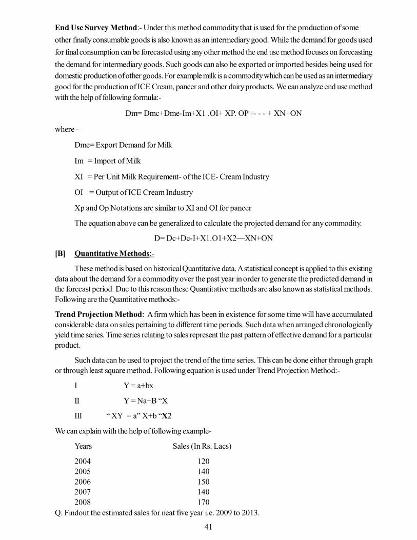
41

End Use Survey Method:- Under this method commodity that is used for the production of someother finally consumable goods is also known as an intermediary good. While the demand for goods usedfor final consumption can be forecasted using any other method the end use method focuses on forecastingthe demand for intermediary goods. Such goods can also be exported or imported besides being used fordomestic production of other goods. For example milk is a commodity which can be used as an intermediarygood for the production of ICE Cream, paneer and other dairy products. We can analyze end use methodwith the help of following formula:-

Dm= Dmc+Dme-Im+X1 .OI+ XP. OP+- - - + XN+ON

where -

Dme= Export Demand for Milk

Im = Import of Milk

XI = Per Unit Milk Requirement- of the ICE- Cream Industry

OI = Output of ICE Cream Industry

Xp and Op Notations are similar to XI and OI for paneer

The equation above can be generalized to calculate the projected demand for any commodity.

D= Dc+De-I+X1.O1+X2—XN+ON

[B] Quantitative Methods:-

These method is based on historical Quantitative data. A statistical concept is applied to this existingdata about the demand for a commodity over the past year in order to generate the predicted demand inthe forecast period. Due to this reason these Quantitative methods are also known as statistical methods.Following are the Quantitative methods:-

Trend Projection Method: A firm which has been in existence for some time will have accumulatedconsiderable data on sales pertaining to different time periods. Such data when arranged chronologicallyyield time series. Time series relating to sales represent the past pattern of effective demand for a particularproduct.

Such data can be used to project the trend of the time series. This can be done either through graphor through least square method. Following equation is used under Trend Projection Method:-

I Y = a+bx

II Y = Na+B “X

III “ XY = a” X+b “X2

We can explain with the help of following example-

Years Sales (In Rs. Lacs)

2004 1202005 1402006 1502007 1402008 170

Q. Findout the estimated sales for neat five year i.e. 2009 to 2013.

42

Calculation of a ,we have equation (II)

Y = NA +b” X720= 5a+0

. . a =720/5 = 144For finding b, we use equation =(III)“XY=a”X+b”X2100= 0+ B10100/0=b .. . b=10By keeping the value of a & b in equation (I)Y = a+bx (a=144, b=10)Y= 144+10X (IV)On the basis of this equation (IV) we can find trend for next five years as follows:-

Years Deviation Sales Y=144+10X(X) (In Rs. Lacs)

2004 -2 -2005 -1 -2006 0 -2007 +1 -2008 +2 -(Already Given)2009 +3 Y(144+10(3)=1742010 +4 1842011 +5 1942012 +6 2042013 +7 214

Solution

Y ears Sales D eviation X2 X Y

(N ) (Y) (X )

2004 120 -2 4 -240

2005 140 -1 1 -140

2006 150 0 0 0

2007 140 +1 1 140

2008 170 +2 4 340

N =5 ? Y =720 ? X =0 ? X2= 10 ? X Y =100

43

Regression Method:- Under this method relationship is established between Quantity demanded andone or more independent variables such as income, price of the related goods, price of the commodityunder consideration, advertisement cost etc. In regression a Quantitative relationship is established betweendemand which is a dependent variable and the independent variable i.e., determinants of demand.

Let us suppose that we have two variables Y and X where Y is dependent on X. it can be expressedin the form of an equation as follows:-

Y=a+bx

We can explain the regression method with the help of following example-

We are required to estimate sales of T.V. if the Index of income rises to 240. The regression equationswill be calculated as follows:

In order to estimate the regression line we should first find the values of the constants a and b

Hence the regression equation isY= a+bx OrY = 5.36+0.66 xIf the Index of Income rises to 240 sales of TV will be estimated as follows:-Y= 53.6+0.66x240 = 53.6+158.4 = 212 Thousand.

Year 2005 2006 2007 2008 2009

I Income 100 110 140 150 200 Index II Sales of 110 130 150 160 180 TV (000)

Y e a r I n c o m e S a le s X 1 Y 1 X 1 2 X 1 Y 1

I n d e x ( X ) o f T Y (Y ) 2 0 0 5 1 0 0 1 1 0 1 0 1 1 1 0 0 1 1 0 2 0 0 6 1 1 0 1 3 0 1 1 1 3 1 2 1 1 4 3 2 0 0 7 1 4 0 1 5 0 1 4 1 5 1 9 6 2 1 0 2 0 0 8 1 5 0 1 6 0 1 5 1 6 2 2 5 2 4 0 2 0 0 9 2 0 0 1 8 0 2 0 1 8 4 0 0 3 6 0 ? X 1 = ? Y 1 ? X 1 2 ? X 1 Y 1 = 7 0 7 3 1 0 4 2 1 0 6 3

36.5=5

)66(.7073n

XΣbYΣ=a

66.0=)70(1042x5

)73x70(1063x5=

XΣ(XΣn)YΣXΣ(YXΣn

=b

11

2

2)12

1

1111

44

Simultaneous Equations Method- This method, also called the complete system approach to forecasting,is the most sophisticated econometric method of forecasting. Since it involves complicated mathematicaland statistical tools, its detail discussion is beyond the scope of this text. Thus the simultaneous equationsmethod overcomes the major problem of the regression method, viz., forecasts for the independent variable.

Graphical Method- Under this method trend is estimated with the help of a graph. Time & Quantitydemanded are taken on both the axis and demand forecasting is made for future. This method is completelysubjective, as in this method graph is drawn and on the basis of this graph demand forecasting is madeExpansion of this graph is completely imaginary & subjective so it can be different for different persons.

According to graphical method, the past data will be plotted on a graph and the indentified trend/behaviour will be extended further in the same pattern to ascertain the demand in the forecast period. Thefollowing diagram shows the past data in bold lines and the forecasted data in dotted lines.

4.7 Demand Forecasting Process

Process for demand forecasting depends on the scope of demand forecasting. We may follow thefollowing sequence in projecting the demand for a product:

1. Specifying the objectives- The person or agency assigned the task of forecasting the demandmust specifiy the purpose for which demand forecasts are being made.

2. Selection of Appropriate Method-Once the purpose of demand forecasting has been specified,we must select the methods which will be used for the purpose.

3. Collection of Appropriate Data-The quality and adequacy of data will determine the quality ofour results and their reliability. As far as possible, data must be collected by experienced persons.

4. Estimation and Interpretation of results- Having collected the relevant data we have to compilethem and obtain results manually or with the help of computers. These results must be interpretedand their correspondence with the objective examined.

5. Evaluation of the Forecasts- If the method or model used in demand forecasting has objectivity;we may expect to receive good results. Yet the result so obtained must be verified by personshaving professional acumen and expertise.

P ast data P ro jected data T rend 1 D em and T rend 2 0 20 02 2 003 20 04 200 5 200 6 200 7 2 008 2 00 9

Forecasting T rend s

45

4.8 Summary

Demand forecasting is the art of predicting demand for a product or service at some future date onthe basis of certain present and past behavior pattern of some related events. The scope of demandforecasting is determined by nature of the product, time period covered and levels of forecasting

The various methods of demand forecasting are opinion survey, trend analysis, regression analysisetc. The choice depends upon number of factors like nature of the product, cost and time requirementsnature of the study etc.


1. What is demand forecasting? Explain its scope and importance.

2. What are the various methods of demand forecasting?

3. Why is forecasting important to business decisions? Discuss the Qualitative and Quantitativemethods of demand forecasting.

4. Explain the various types of methods of demand forecasting.

5. Write short notes on:(A) Trend Method(B) Regression Method(C) Graphic Method

4.10 Suggested Books /References

1. Mathur N.D., Managerial Economics, Shivam book House (P.) Limited, Jaipur2. Mithani, D.M. : Managerial Economics, Himalaya Publishing House, Mumbai

46

Unit - 5 Production FunctionUnit Structure

5.0 Objectives5.1 Introduction5.2 Objective of Production Function5.3 The Production Function5.4 Production Function as Graph5.5 Short Run Production Function5.6 Long Run Production Function5.7 The Law of Variable Proportions5.8 Returns to Scale5.9 Economies of Scale5.10 Summary5.11 Key Words5.12 Self Assessment Test5.13 Suggested Books / References

5.0 Objectives

After studying this unit, you should be able to understand:

• The concept of production function• The objective, assumption and nature of production function• Short run production function• Long run production Function• The law of variable proportions• Returns to scale

5.1 Introduction

Production in economic terms is generally understood as the transformation of inputs into outputs.The inputs are what the firm buys, namely productive resources, and outputs are what it sells. Productionis not the creation of matter but it is the creation of value. Production is also defined as producing goodswhich satisfy some human want. Production is a sequence of technical processes requiring either directlyor indirectly the mental and physical skill of craftsman and consists of changing requiring either directly orindirectly the mental and physical skill of craftsman and consists of changing the shape, size and propertiesof materials and ultimately converting them into more useful articles. Means of production refer to theconcept which combines the means of labor and the subject of labor. Means of labor simply means all thethings which require labor to transform it. Subject of labor means the material to work on. Production,therefore, is the combined resources and equipment needed to come up with goods or services.

Fixed and variable input: An input is the production of goods and services that does not change inthe short run. A fixed input should be compared with a variable input, an input that changes in the short run.Fixed and variable inputs are most important for the analysis of short-run production by a firm. The bestexample of a fixed input is the factory, building, equipment, or other capital used in production. Thecomparable example of a variable input would then be the labor or workers who work in the factory or

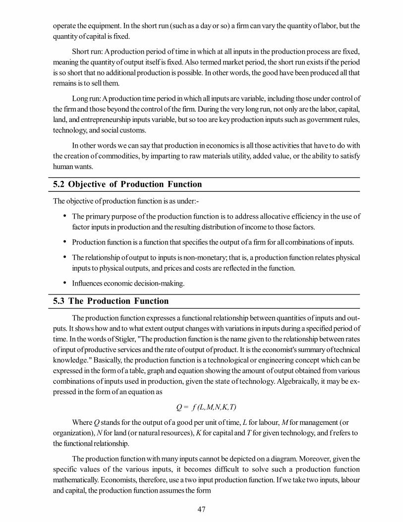
47

operate the equipment. In the short run (such as a day or so) a firm can vary the quantity of labor, but thequantity of capital is fixed.

Short run: A production period of time in which at all inputs in the production process are fixed,meaning the quantity of output itself is fixed. Also termed market period, the short run exists if the periodis so short that no additional production is possible. In other words, the good have been produced all thatremains is to sell them.

Long run: A production time period in which all inputs are variable, including those under control ofthe firm and those beyond the control of the firm. During the very long run, not only are the labor, capital,land, and entrepreneurship inputs variable, but so too are key production inputs such as government rules,technology, and social customs.

In other words we can say that production in economics is all those activities that have to do withthe creation of commodities, by imparting to raw materials utility, added value, or the ability to satisfyhuman wants.

5.2 Objective of Production Function

The objective of production function is as under:-

• The primary purpose of the production function is to address allocative efficiency in the use offactor inputs in production and the resulting distribution of income to those factors.

• Production function is a function that specifies the output of a firm for all combinations of inputs.

• The relationship of output to inputs is non-monetary; that is, a production function relates physicalinputs to physical outputs, and prices and costs are reflected in the function.

• Influences economic decision-making.

5.3 The Production Function

The production function expresses a functional relationship between quantities of inputs and out-puts. It shows how and to what extent output changes with variations in inputs during a specified period oftime. In the words of Stigler, "The production function is the name given to the relationship between ratesof input of productive services and the rate of output of product. It is the economist's summary of technicalknowledge." Basically, the production function is a technological or engineering concept which can beexpressed in the form of a table, graph and equation showing the amount of output obtained from variouscombinations of inputs used in production, given the state of technology. Algebraically, it may be ex-pressed in the form of an equation as

Q = f (L,M,N,K,T)

Where Q stands for the output of a good per unit of time, L for labour, M for management (ororganization), N for land (or natural resources), K for capital and T for given technology, and f refers tothe functional relationship.

The production function with many inputs cannot be depicted on a diagram. Moreover, given thespecific values of the various inputs, it becomes difficult to solve such a production functionmathematically. Economists, therefore, use a two input production function. If we take two inputs, labourand capital, the production function assumes the form

48

Q = f(L, K)

The production function as determined by technical conditions of production is of two types: it maybe rigid or flexible. The former relates to the short run and the latter to the long run.

The Nature of Production Function

The production function depends upon the following factors: a) The quantities of inputs to be used. b) The state of technical knowledge. c) The possible processes of production. d) The size of the firm. e) The prices of inputs.

Now if these factors change the production function automatically changes.

Attributes of Production FunctionThe following are the important attributes of production function: i. The production function is a flow concept. ii. A production function is a technical relationship between inputs and outputs expressed in physical

terms. iii. The production function of a firm depends on the state of technology and inputs. iv. From the economic point of view, a rational firm is interested not in all the numerous possible

levels of output but only in that combination which yields maximum outputs. v. The short run production function pertains to the given scale of production. The long run

production function pertains to the changing scale of production.

5.4 Production Function as Graph

Any of these equations can be plotted on a graph. A typical (quadratic) production function isshown in the following diagram under the assumption of a single variable input (or fixed ratios of inputs sothe can be treated as a single variable). All points above the production function are unobtainable withcurrent technology, all points below are technically feasible, and all points on the function show themaximum quantity of output obtainable at the specified level of usage of the input. From the origin, throughpoints A, B, and C, the production function is rising, indicating that as additional units of inputs are used,the quantity of outputs also increases. Beyond point C, the employment of additional units of inputsproduces no additional outputs (in fact, total output starts to decline); the variable input is being used toointensively. With too much variable input use relative to the available fixed inputs, the company isexperiencing negative returns to variable inputs, and diminishing total returns. In the diagram this isillustrated by the negative marginal physical product curve (MPP) beyond point Z, and the decliningproduction function beyond point C.

Quadratic Production Function

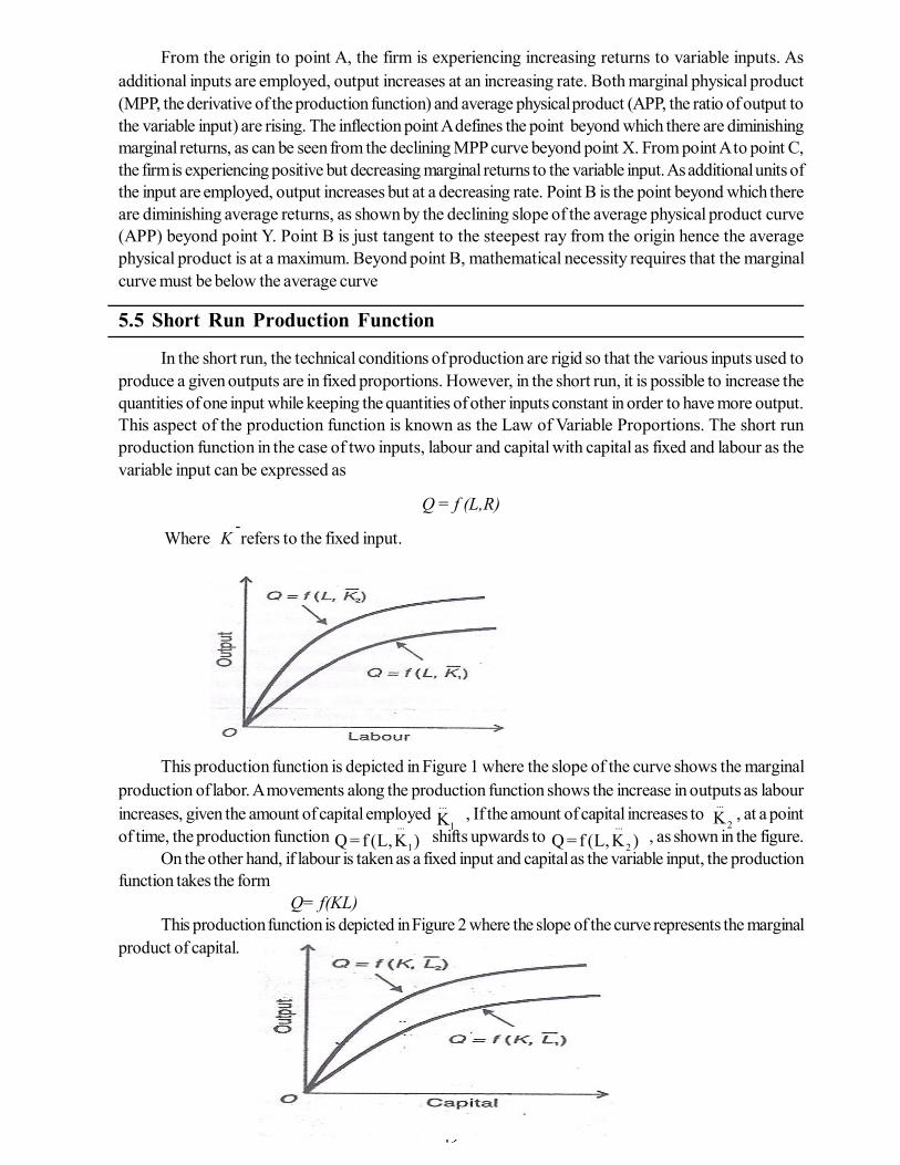
49

From the origin to point A, the firm is experiencing increasing returns to variable inputs. Asadditional inputs are employed, output increases at an increasing rate. Both marginal physical product(MPP, the derivative of the production function) and average physical product (APP, the ratio of output tothe variable input) are rising. The inflection point A defines the point beyond which there are diminishingmarginal returns, as can be seen from the declining MPP curve beyond point X. From point A to point C,the firm is experiencing positive but decreasing marginal returns to the variable input. As additional units ofthe input are employed, output increases but at a decreasing rate. Point B is the point beyond which thereare diminishing average returns, as shown by the declining slope of the average physical product curve(APP) beyond point Y. Point B is just tangent to the steepest ray from the origin hence the averagephysical product is at a maximum. Beyond point B, mathematical necessity requires that the marginalcurve must be below the average curve

5.5 Short Run Production Function

In the short run, the technical conditions of production are rigid so that the various inputs used toproduce a given outputs are in fixed proportions. However, in the short run, it is possible to increase thequantities of one input while keeping the quantities of other inputs constant in order to have more output.This aspect of the production function is known as the Law of Variable Proportions. The short runproduction function in the case of two inputs, labour and capital with capital as fixed and labour as thevariable input can be expressed as

Q = f (L,R)

Where K -refers to the fixed input.

This production function is depicted in Figure 1 where the slope of the curve shows the marginalproduction of labor. A movements along the production function shows the increase in outputs as labourincreases, given the amount of capital employed ...

1K , If the amount of capital increases to ...

2K , at a pointof time, the production function

...

1)K,L(f=Q shifts upwards to ...

2 )K,L(f=Q , as shown in the figure.On the other hand, if labour is taken as a fixed input and capital as the variable input, the production

function takes the form Q= f(KL)

This production function is depicted in Figure 2 where the slope of the curve represents the marginalproduct of capital.

50

A movement along the production function shows the increase in output as capital increases, giventhe quantity of labour employed, L1 . If the quantity of labour increases to L2 , at a point of time, the

production function )L,K(f=Q...

1 shifts upwards to

...

2 )L,K(f=Q

5.6 Long Run Production Function

In the long run all inputs are variable. Production can be increased by changing one or more of theinputs. The firm can changes its plants or scale of production. Equations (1) and (2) represent the long-runproduction function. Given the level of technology, a combination of the quantities of labour and capitalproduces a specified level of output. The long run production function is depicted in Figure 3 where thecombination of OK of capital and OL of labour produced 100Q. With the increase in inputs of capital andlabour to and , the output increases to 200Q. The long run production function is shown in terms of anisoquant such as 100 Q.

In the long run, it is possible for a firm to change all to change all inputs up or down in accordancewith its scale. This is known as returns to scale. The returns to scale are constant when output increases inthe same proportion as the increase in the quantities of inputs. The returns to scale are increasing when theincreased in output is more than proportional to the increase in inputs. They are decreasing if the increasein output is less than proportional to the increase in inputs.

Let us illustrate the case of constant returns to scale with the help of our production function.

Q = (L, M, N, K T2)

Given , if the quantities of all inputs L,M,N,K are increased n-fold the output Q also increasesn-fold. Then the production function becomes

nQ = f(nL, nM, nN, nK )

This is known as linear an homogeneous production function, or a homogeneous function of the firstdegree. If the homogeneous function is of the kth degree, the production function is

nk Q = f(nL, nM, nN, nK)

If k is equal to 1, it is a case of constant returns to scale; if it is greater than 1, it is a case of increasingreturns of scale; and if it is less than 1, it is a case of decreasing returns to scale.

51

Thus a production function is of two types: (i) Liear homogeneous of the first degree in which theoutput would change in exactly the same proportion as the change in inputs. Doubling the inputs wouldexactly double the output, and vice versa. Such a production function expresses constant returns to scale.(ii) Non homogeneous production functions of a degree greater or less than one. The former relates toincreasing returns to scale and the latter to decreasing returns to scale.

5.7 The Law of Variable Proportions

I If one input is variable and all other inputs are fixed the firm's production function exhibits the law ofvariable proportions. If the number of units of a variable factor is increased, keeping other factorsconstant, how output changes is the concern of this law. Suppose land, plant and equipment are thefixed factors, and labour the variable factor. When the number of laborers in increase successivelyto have larger output, the proportion between fixed and variable factors is altered and the law ofvariable proportions sets in. The law states that as the quantity of a variable input is increased byequal doses keeping the quantities of other inputs constant, total product will increase, but after apoint at a diminishing rate. This principle can also be defined thus: When more and more units of thevariable factor are used, holding the quantities of fixed factors constant, a point is reached beyondwhich the marginal product, then the average and finally the total product will diminish. The law ofvariable proportions (or the law of non proportional returns) is also known as the law of diminishingreturns. But as we shall see below, the law of diminishing returns is only one phase of the morecomprehensive law of variable proportions.

Its Assumptions

The law of diminishing returns is based on the following assumptions:1) Only one factor is variable while others are held constant.2) All units of the variable factor are homogeneous.

3) There is no change in technology.

4) It is possible to vary the proportions in which different inputs are combined.

5) It assumes a short run situation, for in the long run all factors are variable.

The product is measured in physical units, i.e. in quintals, tones etc. The use of money in measuringthe product may show increasing rather than decreasing returns if the prices of the product rise, eventhough the output might have declined

Its Explanation

Given these assumptions, let us illustrate the law with the help of Table 1, where on the fixed inputland of 5 acres, units of the variable input labour are employed and the resultant output is obtained. Theproduction function is revealed in the first two columns. The average product and marginal productcolumns are derived from the total product column. The average product per worker is obtained bydividing column (2) by a corresponding unit in column (1). The marginal product is the addition to totalproduct by employing an extra worker. 3 workers produce 36 units and 4 produce 48 units. Thus themarginal product is 12 i.e. (48-36) units.

52

Products increase at first, reach a maximum and then start declining. The total product reaches itsmaximum when 7 units of labour are used and then it declines. The average product continues to rise tillthe 4 the unit while the marginal product reaches its maximum at the 3rd unit of labour, then they also fall.It should be noted that the point of falling output is not the same for total, average and marginal product.The marginal product starts declining first, the average product following it and the total product is the lastto fall. This observation points out that the tendency to diminishing returns is ultimately found in the threeproductivity concepts.

The law of variable proportions is presented diagrammatically in Figure 4. The TP curve first risesat an increasing rate up to point A where its slope is the highest. From point A upwards, the total productincreases at a diminishing rate till it reaches its highest point C and then it starts falling. Point A where thetangent touches the TP curve is called is called the inflection point up to which the total product increasesat an increasing rate and from where it starts increasing at a diminishing rate. The marginal product curve

Table. : Output of Wheat in Physical Units (Quintals)

(1) (2) (3) (4) No. of Total Average Marginal Workers Product Product Product 1 8 8 8 2 20 10 12 Stage I 3 36 12 16 4 48 12 12 5 55 11 7 Stage II 6 60 10 5 7 60 8.6 0 Stage III 8 56 7 -4

53

(MP) and the average product curve (AP) also rise with TP. the MP curve reaches its maximum point Dwhen the slope of the TP curve is the maximum at point A. The maximum point on the AP curves is Ewhere it coincides with the MP curve. This point also coincides with point B on TP curve from where thetotal product starts a gradual rise. When the TP curve reaches its maximum point C the MP curvebecomes zero at point F. When TP starts declining, The MP curve becomes negative. It is only when thetotal product is zero that the average product also becomes zero. The rising, the falling and the negativephases of the total, marginal and average products are in fact the different stages of the law of variableproportions which are discussed below.

Three Stages of Production

Stage - I : Increasing Returns: In stage I the average product reaches the maximum and equalsthe marginal product when 4 workers are employed, as shown in the table 1. This stage is portrayed in thefigure from the origin to point E where the MP curve reaches its maximum and the AP curve is still rising.In this stage, the TP curve also increases rapidly. Thus this stage relates to increasing returns. Here land istoo much in relation to the workers employed. It is, therefore, profitable for a producer to increaseworkers to produce more and more output. It becomes cheaper to produce the additional output.Consequently, it would be foolish to stop producing more in this stage. Thus the producer will alwaysexpand through this stage I.

Causes of Increasing Returns

1. The main reason for increasing returns in the first stage is that in the beginning the fixed factors arelarger in quantity than the variable factor. When more units of the variable factor are applied to afixed factor, the fixed factor is used more intensively and production increases rapidly.

2. In the beginning, the fixed factor cannot be put to the maximum use due to the non applicability ofsufficient units of the variable factor. But when units of the variable factor are applied in sufficientquantities, division of labour and specialization lead to per unit increase in production and the law ofincreasing returns operates.

3. Another reason for increasing returns is that the fixed factors are indivisible which means that theymust be used in a fixed minimum size. When more units of the variable factor are applied on such afixed factor, production increases more than proportionately. This points towards the law ofincreasing returns.

Stage-II : Diminishing Returns: It is the most important stage of production. Stage II startswhen at point E where the MP curve intersects the AP curve which is at the maximum. Then both continueto decline with AP above MP and the TP curve begins to increase at a decreasing rate till it reaches pointC. At this point the MP curve becomes negative when the TP curve begins to decline. Table 1 shows thisstage when the workers are increased from 4 to 7 to cultivate the given land. In Figure 1, it lies betweenBE and CF. Here land is scarce and is used intensively. More and more workers are employed in order tohave larger output. Thus the total product increases at a diminishing rate and the average and marginalproduct decline. This is the only stage in which production is feasible and profitable because in this stagethe marginal productivity of labour, though positive, is diminishing but is not negative. Hence it is notcorrect to say that the law of variable proportions is another name for the law of diminishing returns. Infact, the law of diminishing returns is only one phase of the law of variable proportions. the law ofdiminishing returns in this sense has been defined by Prof. Benham thus: " As the proportion of one factorin a combination of factors is increased, after a point, the average and marginal product of that factor willdiminish."

54

Its Causes : The Law in General Form: But the law of diminishing returns is not applicable toagriculture alone, rather it is of universal applicability. It is called the law in its general form, which statesthat if the proportion, in which the factors of production combin, is disturbed, the average and marginalproduct of that factor will diminish. The distortion in the combination of factors may be either due to theincrease in the proportion of one factor in relation to others or due to the scarcity of one in relation to otherfactors. In either case, diseconomies of production set in, which raise costs and reduce output. Forinstance, if plant is expanded by installing more machines, it may become unwieldy. Entrepreneurial controland supervision become lax, and diminishing returns set in. Or, there may arise scarcity of trained labouror raw material that leads to diminution in output.

In fact, it is the scarcity of one factor in relation to other factors which is the root cause of the law ofdiminishing returns. The element of scarcity is found in factors because they cannot be substituted for oneanother. Mrs Joan Robinson explains it thus: "What the Law of Diminishing Returns really states is thatthere is a limelim it to the extent to which one factor of production can be substituted for another, or, inother words, that the elasticity of substitution between factors is not infinite." Suppose there is scarcity ofjute, since no other fiber can be substituted for it perfectly, costs will rise with production, and diminishingreturns will operate. This is because jute is not in perfectly elastic supply to the industry. If the scarce factoris rigidly fixed and it cannot be substituted by any other factor at all, diminishing returns will at once set in.If in a factory operated by electric power, there being no other substitute for it, frequent powerbreakdowns occur, as is commonly the case in India, production will fall and costs will rise in proportionas fixed costs will continue to be incurred even if the factory works for less hours than before.

According to Wick steed, the law of diminishing returns "is as universal as the law of life itself." Theuniversal applicability of this law has taken economics to the realm of science.

Stage - III : Negative Marginal Returns: Production cannot take place in stage II either for inthis stage, total product starts declining and the marginal product becomes negative. The employment ofthe 8th worker actually causes a decrease in total output from 60 to 56 units and makes the marginalproduct minus 4. In the figure, this stage starts from the dotted line CF where the MP curve is below theX-axis. Here the workers are too many in relation to the available land, making it absolutely impossible tocultivate it.

The Best Stage : In stage I, when production takes place to the left of point E, the fixed factor isexcess in relation to the variable factors which cannot be used optimally. To the right of point F, thevariable input is used excessively in Stage III. Therefore, no producer will produce in this stage becausethe marginal production is negative. Thus the first and third stages are of economic absurdity or economicnonsense. So production will always take place in the second stage in which total output of the firmincreases at a diminishing rate and MP and AP are the maximum, then they start decreasing andproduction is optimum. This is the optimum and best stage of production.

5.8 Returns to Scale

Returns to scale describes the relationship between outputs and scale of inputs in the long run whenall the inputs are increased in the same proportion. In the words of Prof. Roger Miller, "Returns to scalerefer to the relationship between changes in output and proportionate changes in all factors ofproductions." To meet a long run change in demand, the firm increases its scale of production by usingmore space, more machines and laborers in the factory.

55

AssumptionsThis law assumes that1) All factors (inputs) are variable but enterprise is fixed.2) A worker works with given tools and implements.3) Technological changes are absent.4) There is perfect competition.5) The product is measured in quantities.

Explanation

Given these assumptions , when all inputs are increased in unchanged proportions and the scale ofproduction is expanded, the effect on output three stages: increasing returns to scale, constant returns toscale and diminishing returns to scale. They are explained with the help of Table 2 and Fig. 5.

Table 2: Returns to Scale in Physical Units

1. Increasing Returns to Scale

Returns to scale increase because the increase in total output is more than proportional to theincrease in all inputs.

The table reveals that in the beginning with the scale of production of (1 worker +2 acres of land),total output is 8. To increase output when the scale of production is doubled (2 workers + 4 acres ofland), total returns are more than doubled. They become 17. Now if the scale is trebled (3 workers + 6acres of land), returns become more than three-fold, i.e., 27. It show increasing returns to scale. In thefigure RS is the returns to scale curve where R to C portion indicates increasing returns.

U nit Sca le o f Prod uc tio n Tota l Returns

M argina l Re turns

1. 2. 3. 4. 5. 6. 7. 8.

1 workers + 2 Ac res La nd 2 workers + 4 Ac res La nd 3 workers + 6 Ac res La nd 4 workers + 8 Ac res La nd 5 workers + 10 Ac res La nd 6 workers + 12 Ac res La nd 7 workers + 14 Ac res La nd 8 workers + 16 Ac res La nd

8 17 27 38 49 59 68 76

8 Inc reas ing 9 Returns 10 11 C onsta nt 11 Returns 10 D iminis hing 9 Returns 8

56

Causes of Increasing Returns to Scale

Returns to scale increase due to the following reasons:

(i) Indivisibility of Factors : Returns to scale increase because of the indivisibility of the factors ofproduction. Indivisibility means that machines, management, labour, finance, etc. cannot beavailable in very small size. They are available in very small sizes. They are availale only in certainminimum sizes. When a business unit expands, the returns to scale increase because the indivisiblefactors are employed to their maximum capacity.

(ii) Specialization and Division Labour : Increasing returns to scale also result from specialization anddivision of labour. When the scale of the firm is expanded there is wide scope of specialization anddivision of labour. Work can be divided into small tasks and workers can be concentrated to tonarrower range of processes. For this, specialized equipment can be installed. Thus withspecialization, efficiency increases and increasing returns to scale follow.

(iii) Internal Economics: As the firm expands, it enjoys internal economies of production. It may be ableto install better machines, sell its products more easily, borrow money cheaply, procure the servicesof more efficient manager and workers, etc. All these economies help in increasing the returns toscale more than proportionately.

(iv) External Economies: A firm also enjoys increasing returns to scale due to external economies.When the industry itself expands to meet the increased long run demand for its product, externaleconomies appear which are shared by all the firms in the industry. When a large number of firmsare concentrated at one place, skilled labour, credit and transport facilities are easily available.Subsidiary industries crop up to help the main industry. Trade journals, research and training centersappear which help in increasing the productive efficiency of the firms . Thus these externaleconomics are also the cause of increasing returns to scale.

2. Constant Returns to Scale

Returns to scale become constant as the increase in total output is in exact proportion to theincrease in inputs. If the scale of production in increased further, total returns will increase in such a waythat the marginal returns become constant. In the table, for the 4 and 5 the units of the scale of production,marginal returns are 11, i.e., returns to scale are constant. In the figure, the portion from C to D of the RScurve is horizontal which depicts constant returns to scale. It means that increments of each input areconstant at all levels of output.

Causes of Constant Returns to Scale

Returns to scale are constant due to:

(i) Internal Economies and Diseconomies. But increasing returns to scale do not continue indefinitely.As the firm expands further, internal economies are counterbalanced by internal diseconomies.Returns increase in the same proportion so that there are constant returns to scale over a largerange of output.

(ii) External Economies and Diseconomies. The returns to scale are constant when external diseconomiesand economies are neutralized and output increases in the same proportion.

(iii) Divisible Factors. When factors of production are perfectly divisible, substitutable, and homogeneous with perfectly elastic supplies at given prices, returns to scale are constant.

57

3. Diminishing Returns to Scale

Returns to scale diminish the increase in output is less than proportional to the increase in inputs.The table shows that when output is increased from the 6th, 7th and 8th units, the total returns increase ata lower rate than before so that the marginal returns start diminishnig successively to 10, 9 and 8. In thefigure, the portion from D to S of the RS curve shows diminishing returns.

Causes of Diminishing Returns to Scale

Constant returns to scale is only a passing phase, for ultimately returns to sacel start diminishingindivisible factors may become inefficient and less productive. Business may become unwieldy and pro-duce problems of supervision and coordination. Large management creates difficulties of control andrigidities. To theses internal diseconomies are added external diseconomies of scale. These arise fromhigher factor prices or from diminishing productivities of the factors. As the industry continues to expand,the demand for skilled labour, land, capital, etc. rises. There being perfect competition intensive biddingraises wages, rent and interest. Prices of raw materials also group. Transport and marketing difficultiesemerge. All these factors tend to raise costs and the expansion of the firms leads t diminishing returns toscale so that doubling the scale would not lead to doubling the output.

5.9 Economies of Scale

Economies of scale, in microeconomics, refers to the cost advantages that a business obtains dueto expansion. There are factors that cause a producer's average cost per unit to fall as the scale of outputis increased. "Economies of scale" is a long run concept and refers to reductions in unit cost as the size ofa facility and the usage levels of other inputs increase.Diseconomies of scale are the opposite. The com-mon sources of economies of scale are purchasing (bulk buying of materials through long-term contracts),managerial (increasing the specialization of managers), financial (obtaining lower-interest charges whenborrowing from banks and having access to a greater range of financial instruments), marketing (spreadingthe cost of advertising over a greater range of output in media markets), and technological (taking advan-tage of returns to scale in the production function). Each of these factors reduces the long run averagecosts (LRAC) of production by shifting the short-run average total cost (SRATC) curve down and to theright. Economies of scale are also derived partially from learning by doing.

Economies of scale is a practical concept that is important for explaining real world phenomenasuch as patterns of international trade, the number of firms in a market, and how firms get "too big to fail".

58

The exploitation of economies of scale helps explain why companies grow large in some industries. It isalso a justification for free trade policies, since some economies of scale may require a larger market thanis possible within a particular country - for example, it would not be efficient for Liechtenstein to have itsown car maker, if they would only sell to their local market. A lone car maker may be profitable, however,if they export cars to global markets in addition to selling to the local market. Economies of scale also playa role in a "natural monopoly."

An economy of scale exists when larger output is associated with lower per unit cost. Economies ofscale have been classified by Marshall into Internal Economies and External Economies.

Internal Economies are internal to firm when it expands its size or increases its output. They "areopen to single factory or a single firm independently of the action of other firms. They result from anincrease in the scale of output of the firm, and cannot be achieved unless output increases. They are not theresult of invention of any kind, but are due to the use of known methods of production which a small firmdoes not find worthwhile." (A.K. Cairncross)

External Economies are external to a firm which is available to it when the output of the wholeindustry expands. They are "shared by a number of firms or industries when the scale of production in anyindustry or group of industries increases. They are not monopolized by a single firm when it grows in size,but are conferred on it when some other firms grow large". (A.K. Cairncross).

Modern economists distinguish economies of scale in terms of real and pecuniary internal andexternal economies.

Real Internal economies are "associated with a reduction in the physical quantity of inputs, rawmaterials, various types of labour and various types of capital (fixed or circulating) used by a large firm."2Real internal economies which arise from the expansion of a firm are the following:

1. Labour Economies. As the firm expands, it achieves labour economies with increased division oflabour and specialization. When a firm expands in size, this necessitates division of labour wherebyeach worker is assigned one particular job, and the splitting of processes into sub-processes forgreater efficiency and productivity. This, in turn, leads to the increase in the dexterity (skill) of everyworker, the saving time to produce goods, and to the invention of large number of labour savingmachines, according to Adam Smith. Thus division of labour and specialization lead to gratherproductive efficiency and reduction in per unit cost in a large firm.

2. Technical Economies. Technical economies are associated with all types of machines andequipments used by a large firm. They arise from the use of better machines and techniques ofproduction which increase output and reduce per unit cost of production. Technical economies areclassified as follows:

(i) Economies of Indivisibility. Mrs. Joan Robinson refers to economies of factor indivisibility.Fixed capital is one such factor. It is indivisible in the sense that a machine, an equipment or a plantmush be used in a fixed minimum size or capacity to justify its use. Such machines can be mostefficiently used at fairly large output than at small outputs because they cannot be divided intosmaller units. For example, an automated car assembly plant is not a viable proposition, if thenumber of cars to be assembled is small because much of the plant would remain idle. But a largefirm assembling a large number of cars may be able to utilise the plant to its full capacity and achievelower per unit cost.

59

(ii) Economies of Superior Technique. It is only a large firm which can afford to pay for costlymachines and install them. Such machines are more productive than small machines. The high costof such machines can be spread over a larger output which they help to produce. Thus ther per unitcost of production falls in a large firm which employs costly and superior plant and equipment andthereby enjoys a technical superiority over a small firm.

(iii) Economies of Increased Dimensions. The installation of large machines itself brings mayadvantages to a firm. The cost of operating large machines is less than that of operating smallmachines. Even the cost of construction is relatively lower for large machines than for small ones.The cos of manufacture of a double-decker bus is lower as compared to the manufacture of twosingle-decker buses. Moreover, a double-decker carries more passengers than a single-deckerand at the same time requires only a driver and a conductor like the latter. Thus its operating costsare relatively lower.

(iv) Economies of Linked Processes. A large firm is able to reduce itsper unit cost of productionby linking the various processes of production. For instance, a large sugar manufacturing firm mayown its sugarcane farms, manufacture sugar, pack it in bags, transport and distribute sugar throughits own transport and distribution departments. Thus by linking the various processes of productionand sale, a large firm saves the expenses incurred on intermediaries there by reducing unit cost ofproduction.

(v) Economies of the Use of By-products. A large firm possesses greater rosources than a smallfirm and is able to utilise its waste material as a by product. For example, the molasses left over aftermanufacturing sugar from the surgarcane can be used for producing spirit by installing a plant forthe purpose.

(vi) Economies in Power Consumption. A large firm which operates large machines and runsthem continuously, economies in power consumption as compared to small machines.

3. Marketing Economies. A large firm also reaps the economies of buying and selling. It buys itsrequirements of various inputs in bulk and is, therefore, able to secure them at favorable terms in theform of better quality inputs, prompt delivery, transport concessions, etc. Because of its largerorganization, it produces quality products which are offered for sale in attractive packing by itspacking department. It may also have a scale department manned by experts who carry onsalesmanship, propaganda and advertisement through the various media efficiently. Thus a largefirm is able to reap the economies of marketing through its superior bargaining power and efficientpacking and sales organization.

4. Managerial Economies. A large firm can afford to put specialists to supervise and manage thevarious departments. There may be a separate head for manufacturing, assembling, packing,marketing, general administration, etc. This decentralization leads to functional specialization whichincreases the productive efficiency of the firm. "Large firms apply techniques of managementinvolving a high degree of mechanization, such as telephones, telex machines, television screens andcomputers. These techniques save time in decision making process and speed up to processing ofinformation, as well as increasing its amount and its accuracy." These managerial economies alsoreduce per unit cost of management because with expansion of the firm, the various departmentalmanagers will manage large output as efficiently as they were managing small output at the samesalary.

60

5.10 Summary

Production function is an equation that asserts the relationship between the quantities of productivefactors used and the maximum amount of product obtained at certain technological level. The productionfunction can thus measure the marginal productivity of a particular factor of production and determine thecheapest combination of productive factors. Some inputs can be varied flexibly in a relatively short periodof time. We conventionally think of labor and raw materials as "variable inputs" in this sense. Other inputsrequire a commitment over a longer period of time.We have seen that the concept of marginal productivityand the law of diminishing marginal productivity play central parts in both the efficient allocation ofresources in general and in profit maximization.

5.11 Key Words

• Production Function: In micro-economics, A production function is a function that specifies theoutput of a firm, an industry, or an entire economy for all combinations of inputs.

• Law of variable proportions: I n economics, diminishing returns (also called diminishingmarginal returns) refer to how the marginal production of a factor of production starts to progres-sively decrease as the factor is in creased, in contrast to the increase that would otherwise benormally expected.

• The law of returns to scale: An economic concept referring to a situation in which economies ofscale no longer function for a firm. Rather than experiencing continued decreasing costs perincrease in output, firms see an increase in marginal cost when output is increased.

• Economies of Scale : Economies of scale, in microeconomics, are the cost advantages that abusiness obtains due to expansion. They are factors that cause a producer's average cost per unit tofall as scale is in creased.


1 What do you mean by production? Define production function and describe the assumptions.

2 What are fixed and variable inputs?

3 Distinguish between laws of return to variables proportion and laws of returns to scale

4 How will you define economy of scale?

5 What do you mean by internal and external economy of scale?

5.13 Suggested Books /References

1. Mathur N.D., Managerial Economics, Shivam book House (P.) Limited, Jaipur

2. Mishra & Puri : Managerial Economics, Himalaya Publishing House, Mumbai

61

Unit – 6 Cost Concepts and AnalysisUnit Structure

6.0 Objectives6.1 Introduction6.2 Cost Function6.3 Determinants of Costs6.4 Cost Concepts6.5 Components of Costs6.6 Short Run Cost Function6.7 Long-Run Average Cost Curve6.8 Summary6.9 Key Words6.10 Self Assessment Test6.11 Suggested Books / References

6.0 Objectives

The studying this unit, you should be able to understand:

• The Concept of cost• Different cost concepts• Cost function• Determinats of cost• Components of cost

6.1 Introduction

It is necessary for the proper understanding of cost analysis, to know various cost concepts that areoften employed. When an entrepreneur decides to produce a commodity, he has to pay the price forinputs which he uses in production. When he employes labour, he pays wages to them and pays moneywhen buys raw materials, fuel and power, rent for the factory building and so on. All these are included incost of production. The kind of cost concept used in a particular situation dependes on cost of production.The kind of cost concept used in a particular situation depends upon the business decision that themanagement makes. An accountant will take into account only the payments and charges made by themanager to the suppliers of various productive inputs, but the managerial economist views the cost insome what different form. The cost estimates made by contentional, financial accounting are not appropriatefor all managerial uses, Further different problems call for different kinds of costs, therefore it is necessaryto have a complete understanding of different cost concepts for clear business thinking.

6.2 Cost Function

Cost function is derived from the production function. Time factor is very important in cost theory.The short-run costs are the costs over a period during which some factors of production are fixed. Thelong-run costs are the costs over a period long enough to permit changes in all factors of production. Bothin the short-run and in the long-run, cost is a multivariate function, i.e., it is determined by many factorssimultaneously, symbolically, the long run cost function is given as:

62

C = f(X,T,Pf)

And the shot-run-run cost function is:

C = f(X, T, Pf, K)

Where C = Total Cost

X = OutputT = TechnologyPf = prices of factorsK = Fixed factor (s)

Graphically, the cost function is generally shown on a two-dimensional diagram by taking C= f(x),ceteris paribus, If other factors (i.e.T,Pf) to change, then the cost curve will shift.

6.3 Determinants of Costs

Factors determining the cost are

(a) Size of plant: There is an inverse relationship between size of plant and cost. As size of plantincreases, cost falls and vice versa.

(b) Level of Output: There is a direct relationship between output level and cost. More the level ofoutput, more is the cost ( i. e., total cost) and vice Versa.

(c) Price of Inputs: There is a direct relationship between price of inputs and cost. As the price ofinputs rises, cost ruses and vice versa.

(d) State of technology: More modern and upgraded the technology implies lesser cost and viceversa.

(e) Management and administrative efficiency: Efficiency and cost are inversely related. Morethe efficiency in management and administration better will be the product and less will be the cost.Cost will case of inefficiencies in management and administration.

6.4 Cost Concepts

According to Marshall, the real cost of production includes the “real cost of efforts of variousQualities” and “real cost of waiting”

It is also known as “alternative sacrificed cost, or “transfer cost”. Opportunity cost of a commodityis the alternative sacrificed in order of order to order to obtain it.

Cost concepts differ because of differences in view point. Different combinations of cost ingredientsare important for various kinds of management problems. Disparities occur form deletions, from additionsfrom recombination which do not appear anywhere in the accounting records. Different cost conceptsexplained in our study are

(a) Actual cost and opportunity costs(b) Past and future costs(c) Short run and long run costs(d) Variable or Prime cost and fixed costs or supplementary costs

63

(e) Incremental costs and sunk costs(f) Traceable and Non-Traceable costs(g) Explicit and Implicit costs(h) Controllable and Non-Controllable Costs(i) Private, External and social costs(j) Total. Average and Marginal Costs

(a) Actual Cost and Opportunity Cost

Actual costs are those that involve financial expenditure incurred for acquiring inputs for producinga commodity. These expenditures are recorded in the books of accounts of the firm. The expenditures arewages, payment made for the purchase made for the purchase of raw materials machinery etc. Thesecosts are called actual costs or outlay costs or real costs. The real cost of production has been interpretedin different forms. According to Adam Smith, “Pains and sacrifices of labour are real cost of production”Opportunity cost is not the actual expenditure but it is the revenue earned by employing that good orservice in some other alternative uses. Opportunity cost is the cost of producing any commodity in the nextbest alternative cost. For example the inputs which are used to manufacture a car may also be used in theproductions of military equipment. A farmer who is producing paddy can also produce sugar cane with thesame factors. Therefore, the opportunity cost of one quintal of paddy is the amount of sugarcane given up.Main points of opportunity cost are:

1. The opportunity cost of any commodity is only the next best alternative forgone.2. The next best alternative commodity that could be produced with the same value of the factors,which are more or less the same.3. It helps in determining relative prices of factor inputs at different places.4. It helps in determining the remuneration to services.5. It helps the manager to decide what he should produce in the factory.

(b) Past and Future Costs

Past costs are actual costs incurred in the past. These costs are mentioned in the financial accounts.Future costs are those costs which are to be incurred in the near future. This is only a forecast. Futurecosts matter for managerial decisions because, the management can evaluate the desirability of thatexpenditure, since the past costs are costs that have already been incurred, and there is no scope formanagerial decision. If the management finds out that the past costs are excessive, it cannot do anything torectify it now. In the case of future costs, if the management considers them very high , it can either reducethem or postpone the use of them.

(c) sort Run and Long Run Costs

Shorts run costs are those associated with variation in the utilization of fixed plan or other facilities,whereas long run costs encompass changes in the size and kind of plant. Short run cost is relevant when afirm has to decide whether or not to produce more or less with the given plant and equipments. If the firmdicides to expand the capacity of the plant, it must examine the long run cost. Long run cost is useful inmaking investment decisions.

(d) Prime or Variable Costs and Supplementary or Fixed Costs

Prime costs are variable or direct costs. Normally, they include the money cost of the raw materialused in making a commodity, the wages of the labour directly spent on it and the extra wear and tear of the

64

machine that makes it. Suppose a carpenter has been asked to charge for a chair, he would first think ofthe wood and cane that he used and the number of days he spent in making it. This is the prime cost.

It is clear that prime cost of a commodity differs with the quantity produced. When more chairs aremade, more money will have to be spent on carpenter’s wages as well as on wood. When production isstopped, the prime costs disappear. Prime costs therefore are also called the Variable Costs.

Supplementary or Fixed Costs

The carpenter will not only charge for the chair but also for the wood and his wage. In addition tothe above he will think of including a portion of rent in the cost that he is paying and also interest on thecapital invested, the municipal taxes, etc. A big company will further have to include a portion of thesalaries of the manager, the peons, the cost of advertisement and salesmanship, etc. These costs must alsobe covered. They are called supplementary costs on costs or over head charges or fixed costs.

The fixed costs do not change with the volume of production. Irrespective of quantity of goodsproduced, big or small, the charges on account of rent, taxes, interest salaries, etc will be included. Evenif the orders cease to flow in and the factory is closed, these costs will continue. They are fixed costs.

Generally, the distinction between the variable and fixed costs applies only to the short period,because nothing can really remain fixed in the long run. In the long the strength and the salary bill of the staffmay change, the amount of capital invested may be different, hence the amount of interest would vary.Thus, all costs, which ware regarded as fixed in the short run, may vary in the long run. Thus in the longrun, all costs are variable.

(e) Incremental Costs and Sunk Costs

Incremental costs are the added costs of a change in the level of production or the nature of activity.It may be adding a new product or changing distribution channel, or adding new machinery, etc. It appearsto be similar to marginal cost, but it is not managerial cost. Marginal cost refers to the cost on added unitof output.

Sunk costs are costs which cannot be altered in any way. Sunk costs are costs which have alreadybeen uncured. For example, cost incurred in constructing a factory. When the factory building is constructedcosts have already been incurred. The building has to be used for which originally envisaged. It cannot bealtered when operations are increased or decreased. Investment on machinery is an example of sunk cost.

The distinction between the sunk cost and the incremental cost is important in evaluating the alterative.Incremental cost will be different in the case of different alternative. Hence incremental cost is relevant forthe management in decision making. Sunk cost will remain the same irrespective or the alternative indecision making. Sunk cost will remain the same irrespective of the alternative selected. Marketingprogramme has its own set of incremental costs for equipment, delivery men and executive time and so on.

(f) Traceable Costs and Non-traceable Costs

Traceable costs are those which can easily be identified by a producing unit. These are directlyrelated to a unit of operation like a product, a process or department of firm. These are also know asdirect costs or assignable costs.

65

Non-traceable costs or indirect costs are not traceable to plant, department or unit or operation orindividual final product. Fox example, for operating air-services, the cost of runway, airport equipment,staff, etc. cannot be assigned to one passenger. These are common costs to distinguish between traceableand non-traceable costs. Change in the total output and product-mix affect the total costs in complexways. Even a traceable cost gets lost in the process and has to be indentified as overhead cost only.

(g) Explicit Cost and Implicit Costs

The total cost of production of a particular commodity can be said to include ‘Expenditure’ or‘explicit’ cost, ‘non-expenditure’ or ‘implicit’ cost. Explicit costs are paid by the employer to owners ofthe factor units, which do not belong to the employer himself. These costs include payments for rawmaterials interest on borrowed funds, rent on hired land and taxes paid to the government.

Non-expenditure or implicit costs arise when factor units are owned by the employer himself, Thetwo non expenditure costs are supplied by the shareholders; in the case of small business units thedepreciation and an average or normal return on the money capital wages of the entrepreneur or organizerhimself will have to be included in this category.

Expenditure costs are explicit since they are paid to factors outside the firm while non-expenditurecosts are implicit and hence they are imputed costs.

(h) Controllable Costs and Non-Controllable costs

Controllable costs are those that cannot be controlled by some executive action on the part of themanagement These can improve the efficiency of the factor inputs.

Non-controllable costs are those that cannot be controlled through any administrative or supervisoryaction. These tend to wastage of resources and encourage inefficiency.

(i) Private, External and Social Costs

Some times, there is a discrepancy between the cost incurred by a firm and the cost that must beincurred by the society as a whole. For example, a factory may dispose of its untreated waste into a riveror a lake. Such a method of waste disposal may minimize the private cost but it does impose a cost to thesociety in the form of polluted waterways. A cost that is not borne by the firm, but is incurred by others insociety is called an external cost. The true cost to the society must include all costs regardless of whobears them. Thus, the social cost is the sum of private and external cost. This is

Social cost = Private Cost + External Cost Or

External Cost = Social Cost- Private Cost

(j) Total, Average and Marginal Costs

Total cost is made up of both the fixed cost and the variable cost. They are represented in thefollowing diagram. OX and OY are the two axes, along OX is represented the quantity produced andalong OY the cost. FC, a straight horizontal line represents the fixed cost and the area above is thevariable cost so that the TC is total cost curve.

66

Fixed Cost, Variable Cost, Total Cost Curves

Average cost at any output outputofUnitsCostTotal

=

Average Cost: Average cost is the sum of average variable cost and average fixed cost; it is also calledaverage total cost. If the totalcost of producing 60 units of good is 2400 rupees, then average cost.will be

20=1202400

Marginal Cost : Marginal cost is the cost of producing an additional unit of output. In other words,marginal cost is the addition made to the total cost by producing one more unit of output. for example, ifthe total cost of producing 120 units is 2400 rupees and the total cost of producing 121 units is 2436rupees, the marginal costing in this case will be equal to 36 rupees.The concepts of total cost, averagecost and marginal cost can be understood easily form the following table;

Total, Average and Marginal Costs

Output Total Cost Average Cost Marginal costRs. Rs. Rs.

1. 60 60 602. 80 40 203. 90 30 104. 96 24 65. 100 20 46. 144 24 447. 210 30 668. 320 40 1109. 540 60 22010. 900 90 360

It is evident from the above table that marginal cost of the second unit has been derived fromsubtracting Rs60 from Rs80 (80-60) =20. Marginal costs of subsequent units are obtained in the samemanner. Hence Marginal cost is the addition made to the total cost at each step.

Y

XO

FC

Variable Cost

Fixed Cost

TC

Quantity

Cost(Rs.)

Total Cost

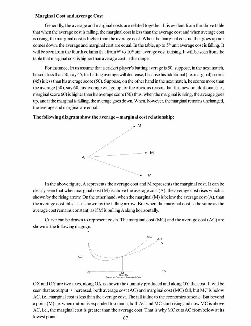
67

Marginal Cost and Average Cost

Generally, the average and marginal costs are related together. It is evident from the above tablethat when the average cost is falling, the marginal cost is less than the average cost and when average costis rising, the marginal cost is higher than the average cost. When the marginal cost neither goes up norcomes down, the average and marginal cost are equal. In the table, up to 5th unit average cost is falling. Itwill be seen from the fourth column that from 6th to 10th unit average cost is rising. It will be seen from thetable that marginal cost is higher than average cost in this range.

For instance, let us assume that a cricket player’s batting average is 50. suppose, in the next match,he scor less than 50, say 45, his batting average will decrease, because his additional (i.e. marginal) scores(45) is less than his average score (50). Suppose, on the other hand in the next match, he scores more thanthe average (50), say 60, his average will go up for the obvious reason that this new or additional (i.e.,marginal score 60) is higher than his average score (50) thus, when the marginal is rising, the average goesup, and if the marginal is falling, the average goes down. When, however, the marginal remains unchanged,the average and marginal are equal.

The following diagram show the average – marginal cost relationship:

In the above figure, A represents the average cost and M represents the marginal cost. It can beclearly seen that when marginal cost (M) is above the average cost (A), the average cost rises which isshown by the rising arrow. On the other hand, when the marginal (M) is below the average cost (A), thanthe average cost falls, as is shown by the falling arrow. But when the marginal cost is the same as theaverage cost remains constant, as if M is pulling A along horizontally.

Curve can be drawn to represent costs. The marginal cost (MC) and the average cost (AC) areshown in the following diagram.

OX and OY are two axes, along OX is shown the quantity produced and along OY the cost. It will beseen that as output is increased, both average cost (AC) and marginal cost (MC) fall, but MC is belowAC, i.e., marginal cost is less than the average cost. The fall is due to the economics of scale. But beyonda point (M) i.e. when output is expanded too much, both AC and MC start rising and now MC is aboveAC, i.e., the marginal cost is greater than the average cost. That is why MC cuts AC from below at itslowest point.

A

M

M

M

Y

XO

MC

QuantityAverage Cost and Marginal Cost

Cost

M

AC A

68

6.5 Components of Costs

Classification of total cost on the basis of the cost fixed and variable inputs is not enough for takingmanagerial decisions. A firm has to work out in detail the different expenses that it incurs on various heads.In order to compute profit and loss a form has to analyse the ‘components’ or ‘elements’ of total cost.

Functionally, the major components of the total cost of a product the comprises the total costs canbe divided as follows:

(i) Prime Cost = Direct Material + Direct Wages + Direct Expenses(ii) Production Overhead = Indirect Material + Indirect Wages + Indirect Expenses(iii) Production cost = Prime Cost + Production overhead(iv) Costs Related to = General Administration = Marketing/Sales = Research = Development(v) Total = Production Cost + Costs Related to other functions

The difference between total revenue and total cost revenue and total cost represents profits orloss. In case, the TR is move than the cost of sales the firm gets profit, while if TR is less than the cost ofsales the firm suffers loss.

6.6 Short Run Cost Function

The short-run refers to that period of time within which a firm can vary its output by varying only theamount of variable factors, factors such as labour and raw material. In the short run period the firm cannotalter the fixed factors such capital equipment management personal, the factory buildings etc. Suppose afirm wants to increase production in the short run it can do so only by hiring more worker or buying andusing more raw materials. In the short run a firm cannot enlarge the size of the existing plant or build a newplant of a bigger capacity. Thus in the short run only variable factors can be varied while the fixed factorsremain the same.

COMPONENTS OF COSTS

Costs Related to the Production Function Costs Related to other Functions

MATERIAL USED WAGES EXPENSES

DIRECT INDIRECT

Material Wages Expenses Material Wages Expenses

Prime Cost Production overhead

Production Cost

Total Cost

GeneralAdministrationMarketing/SalesResearchDevelopment

69

Short-run Fixed and Variable Costs

In the period, the prime costs relating to lobour and raw material can be varied whereas the fixedcosts remain the same. On the other hand, in the long period, even the fixed costs relating to plant andmachinery, staff salaries, etc, can be varied. That is, in the long run all costs are variable and no costs arefixed.

Short-run Cost Curve

Generally, in the short-run a firm will adjust output to demand by varying the variable factors. Whenthe factors of production can be used in varying proportions, it means that the scale of operations of thefirm can be changed. Each time the scale of operations is changed, a new short-run curve will have to bedrawn for the firm such as SAC’ SAC” and SAC” in the next.

Suppose, a firm has the short-run cost curve SAV”. In this case, the optimum will be OM’. Whenit wants to increase the output to OM” in the short-run it can be obtained at the average cost M”L” alongthe short-run cost curve Sac:, because in the short-run the scale of operation is fixed.

On the other hand, during the long run, a new and bigger plant can be built on which OM” is theoptimum output. That is, the firm has now a short run average cost curve SAC”, and by increasing thescale of its operations, the firm can produce the OM” output at a cost of M”L” instead of M”L”.

It is evident form the above figure that at any scale of operations in the short-run, a firm will haveregions of rising and falling costs. On the other hand, in the long-run the firm can produce on a completelyshort-run cost curve, and there will be an output where the average cost is minimum. This is the optimumoutput.

6.7 Long-Run Average Cost Curve

In the following diagram SAC’, SAC” and SAC”’ refer to the short run cost curve correspondingto the different scales of operations. In the following situations the firm will be producing the desired outputat the lowest cost. For example. OM output is produced at PM in the scale of operations represented bythe curve SAC. OM will be produced on SAC, and so on.

Y

XO

OutputShort-run Cost Curve

Cost

M’ M’’

L’’L’’’

L’

SAC’SAC’’ SAC’’’

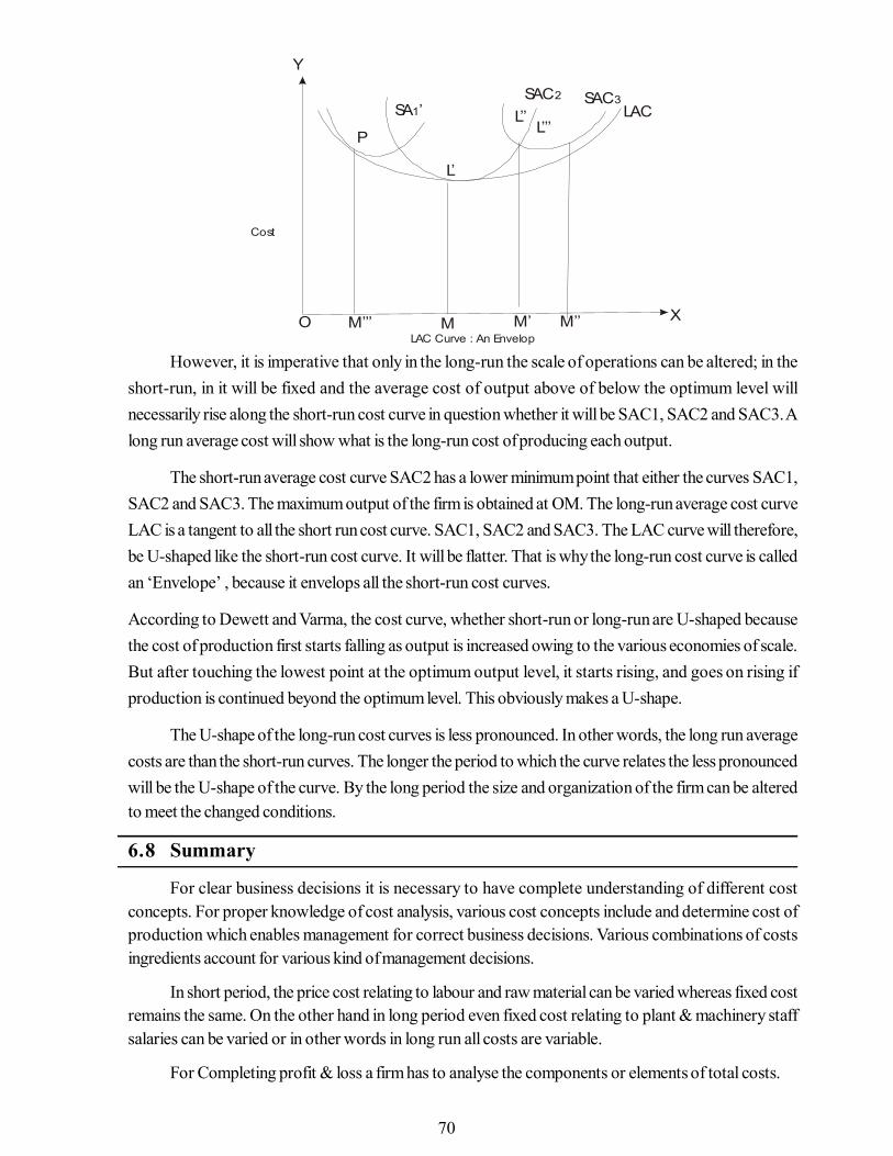
70

However, it is imperative that only in the long-run the scale of operations can be altered; in theshort-run, in it will be fixed and the average cost of output above of below the optimum level willnecessarily rise along the short-run cost curve in question whether it will be SAC1, SAC2 and SAC3. Along run average cost will show what is the long-run cost of producing each output.

The short-run average cost curve SAC2 has a lower minimum point that either the curves SAC1,SAC2 and SAC3. The maximum output of the firm is obtained at OM. The long-run average cost curveLAC is a tangent to all the short run cost curve. SAC1, SAC2 and SAC3. The LAC curve will therefore,be U-shaped like the short-run cost curve. It will be flatter. That is why the long-run cost curve is calledan ‘Envelope’ , because it envelops all the short-run cost curves.

According to Dewett and Varma, the cost curve, whether short-run or long-run are U-shaped becausethe cost of production first starts falling as output is increased owing to the various economies of scale.But after touching the lowest point at the optimum output level, it starts rising, and goes on rising ifproduction is continued beyond the optimum level. This obviously makes a U-shape.

The U-shape of the long-run cost curves is less pronounced. In other words, the long run averagecosts are than the short-run curves. The longer the period to which the curve relates the less pronouncedwill be the U-shape of the curve. By the long period the size and organization of the firm can be alteredto meet the changed conditions.

6.8 Summary

For clear business decisions it is necessary to have complete understanding of different costconcepts. For proper knowledge of cost analysis, various cost concepts include and determine cost ofproduction which enables management for correct business decisions. Various combinations of costsingredients account for various kind of management decisions.

In short period, the price cost relating to labour and raw material can be varied whereas fixed costremains the same. On the other hand in long period even fixed cost relating to plant & machinery staffsalaries can be varied or in other words in long run all costs are variable.

For Completing profit & loss a firm has to analyse the components or elements of total costs.

Y

XOLAC Curve : An Envelop

Cost

M’M’’’

L’’L’’’

L’

SA ’1SAC2 SAC3

LAC

P

M’’M

71

6.9 Key Words

• Short run cost: Cost over a period during which some factors of production are fixed.

• Long run cost: Cost over a long period to permit changes in all factors of production.

• Post costs: Actual costs incurred in the past.

• Future costs: Which are to be incurred in near future.

• Prime costs: Refers to variable or direct costs.

• Incremental cost: Added cost of a change in the level of production.

• Sunk cost: Which have all ready been incurred and cannot be altered.

• Traceable cost: Which are easily be identified by a producing unit.

• Non Traceable cost: Which are not traceable to plant, department of unit of operation.

• Explicit cost & inexplicit cost: Total cost of production of a commodity can be said to includeexpenditure explicit cost and non expenditure or inexplicit cost.

• Controllable cost: That can be controlled by some executive action in the part of management.

• Non Controllable cost: That can not be controlled through any administrative or supervisoryaction.

• Total Cost: Made up of both fixed and variable cost.

• Average Cost: Product of total cost to units of output or sum of average variable cost and fixedcost.


1. Discuss briefly the different cost concepts.

2. Explain the determinants of costs.

3. Distingusish between:(a) Fixed and variable cost(b) Average and implicit cost(c) Explicit and Implicit cost

4. Firm plans in long run and operate in short run. Explain.


1. Mathur N.D.: Managerial Economics, Shivam Books House (P.) Limited, Jaipur

2 Adhikari M.: Managerial Economics, Khosla Educational Publisher, New Delhi.

72

Unit - 7 Market StructureUnit Structure

7.0 Objectives7.1 Introduction7.2 Objective of Market Structure7.3 Classification of Market7.4 Market Structure7.5 Summary7.6 Key Words7.7 Self assessment Test7.8 Suggested Books / References

7.0 Objectives


• The concept of market• The saliant features of market• Classification of market• Concept of market structure• Types of market structure• The issues in market structure

7.1 Introduction

In general, market means a place where there are many buyers and sellers of different productswho are actively engaged in buying and selling acts. The firm's demand curve is expected to depend onsuch things as the numbers of sellers in the market and the similarity of their products. These are theaspects of market structure which may be termed as the characteristics of market of generalisation that arelikely to influence a firm's behaviour and performance. In broader sense face to face contact betweenbuyers and sellers is not necessary. They can establish contact through different means of communicationlike letters, agents, telegraphs, telephone etc. or newspapers. Thus, the terms market does not mean andparticular place but the entire area where buyers and sellers of a commodity are in such close contact witheach other that the price of the same commodity tends to be one throughout that area.

According to Cournot, "Economists understand by the term market not any particular market placein which things are bought and sold but the whole of any region in which buyers and sellers are in such freeintercourse with each other that the price of the same goods tends to uniformity, easily and quickly."

According to J.C. Edwards, "A market is that mechanism by which buyers and sellers are broughttogether. It is not necessarily a fixed place."

Chapman defines as "The term market refers not necessarily to place but always to a commodityand the buyers and sellers who are in direct competition with one another."

7.2 Objective of Market Structure

Market Structure influences how a firm behaves in pricing, supply, barrier of entry, efficiency, com-petition.

73

• It enables an organisation to control its market plan.

• Market Structure helps in strategic decision making.

• Market Structure aligns the organisation to the changed environment.

• Market Structure is important and it affects market outcomes through its impact on motivation,opportunities & decision of economic factors.

On the basis of above mentioned definition following characteristics can be brought out:

1- Area: Market does not mean any particular place where buyers and sellers meet, rather, it meansthe entire area within which buyers and sellers are spread and have close contacts with each other.For example Bata Shoes has market all over India., because its buyers and sellers are found inevery city and state.

2- Buyers & Sellers: For exchange at least one buyer and one seller are needed. Thus, the existence ofbuyers and sellers is a must. If one of the two does not exist in a region, it does not satisfy thefunction of market. It is not necessary that buyers and sellers should be physically present to ex-change or transact the things. They can come in contact through correspondence.

3- One Commodity: For the existence of the market there must be one commodity like wheat, sugar,ghee, vegetables and utensils. Thus they can be termed as wheat market, sugar market, ghee mar-ket, vegetables market, utensils market respectively.

4- Free Competition: There must be healthy and free competition among the buyers and sellers. Thusin practice, there should not be any restrictions on them. There must be free competition.

5- One Price: Generally it is remarked that in a market one price prevails which is the main feature andtestimony of a market.

7.3 Classification of Market

(1) On the basis of area or region:

The economists have classified the market on the basis of area or region which further can besummarised as under.

(i) Local Market(ii) Regional or Provincial Market(iii) National Market(iv) International Market

(i) Local Market: If the buyers and sellers of a certain commodity are limited to certain area orregion, then it is called local market. The perishable goods and low price goods have their localmarket like milk, ghee, hand-made fans, basket, cots etc.

(ii) Regional or Provincial Market: If the buyers and sellers of a commodity are confined to certainregion, say a province like Rajasthan or Haryana, then it is known as regional or provincial market.The area of regional market is greater than that of local market e.g. the demand for Red Bangles inRajasthan or the demand for Laharia in Rajasthan.

(iii) National Market: When the buyers and sellers are not confined to state boundary, but are

74

spread throughout the country e.g., the market of sarees and dhotis or of Gandhian cap or of Nehrucut jacket etc. have national market. These are demanded throughout the nation. Hence they comeunder the purview of national market.

(iv) International Market: When the buyers and sellers are spread across the geographical bound-ary of a nation and the demand for such product is worldwide or universal demand then its marketis known as international market e.g. market for gold and silver.

(2) On the basis of time:

On the basis of time the economist have classified the market as under:

(i) Very short period Market.(ii) Short period Market.(iii) Long period Market.(iv) Very long period Market.

(i) Very short period Market: This market can further be classified into Daily Market or Weeklymarket. Very short period market is that market which takes part in transaction for a very shortperiod of time say a few hours a day or so. In very short period the supply of the product cannot beincreased e.g. of milk. Here the demand determines the price. In very short period market generallyperishable commodities are exchanged.

Daily Market- The market for perishable commodities come under daily market e.g. milk andvegetables.

Weekly Market- Sometimes a market operates on any specific day of week. It is generally foundin those areas in which main market has its closed day for the week, say Sunday market, or Tuesdaymarket or whatever the case may be according to the closing day of the main market.

(ii) Short period Market: Its time period is greater than that of the previous one in which the supplyof the product can be increased but we cannot make any change in production plant according tothe changed demand. In short period also the demand side plays a major role in determining theprice as change in the plant and machinery is not possible from the point of view of production.

(iii) Long Period Market: It is such a market in which we can make necessary changes in the plantand machinery as well to increase the supply of the product according to its demand. The supply ofthe product plays a vital role in price determination resulting in normal price for the product in suchmarket.

(iv) Very long period Market: There can be an enormous change in the supply of the product invery long period market. New techniques of production, innovations and the new models of prod-ucts can be produced because of a very long period. And in very long periods the demand alsoincreases because of change in population, habits, customs, fashions etc.

(3) On the basis of Functions:

On the basis of functions the markets can be classified as under:

(i) Mixed or general Market.(ii) Specialised Market(iii) Marketing by samples.(iv) Marketing by grading.

75

(i) Mixed or general Market: When different types of commodities are transacted simultaneously ina market then it is known as mixed or general market e.g. Chandni Chowk market in Delhi.

(ii) Specialised Market: When only one product or any of the special product is transacted in amarket then it is known as specialised market. In such market, a particular thing is traded with itsdifferent brand names of possibly different kinds, e.g. bathing soap is bought and sold in soapmarket could be Lux, Liril, Hamam, Rexona, Lifebuoy, etc.

(iii) Marketing by Samples: In such market the firms need not show whole of their product. Theyonly send samples through their agents or they may themselves show the samples of their product,e.g. in case of wool, cloth, paints etc.

(iv) Marketing by Grading: The product is first graded according to its quality and then put forth forselling is known as marketing by grading e.g. in an Agricultural product market the product isgraded accordingly and then sold. It is known as Marketing by grading.

(4) On the basis of nature of commodity:

The market can also be classified on the basis of nature of commodity.

(i) Product Market.(ii) Stock Market.(iii) Bullion Market.

(i) Product Market: The production goods are exchanged in these market e.g. Agriculture productis bought and sold in Agriculture produce market.

(ii) Stock Market: Stock market is a market where stock and shares, bonds, securities, debenturesetc. are bought and sold. Bulls and Bears do transactions in the stock market as per their marketreading.

(iii) Bullion Market: This is such a market in which Metallic trading exists e.g. the goods like silverand gold better known as Bullion are traded and transacted.

(5) On the basis of Legality:

On the basis the market can be sub-divided as under:

(i) Legal or fair Market.(ii) Illegal Market.

(i) Legal and Fair Market: When the goods are transacted in a market under certain norms andrules, the market is known as legal market which also has a legal sanctity behind it issued by thelegal authorities in a country. Here every consumer gets commodities at fair prices. These marketsare also known as Fair Market.

(ii) Illegal Market: When the transaction of certain commodities is taking place in more than or lessthan quantity prescribed by the legal authorities in operation say a government and then it is termedas illegal trade. The Hong Kong Market is an illegal market at International level. Generally it is alsotermed as Chor Market.

76

CLASSIFICATION OF MARKET

The economists have classified the market on the basis of following elements.

General classification of market

7.4 Market Structure

The level of production of any commodity depends upon structure of its market. Possible outcomesof sales, revenues, profits are prices and structured under market structures. The firms demand curve tothe industry demand curve is expected to depend on such things as the number of sellers in the market andthe similarity of their products. These are aspects of market structures which may be called characteristicsof market or generalization that are likely to influence firm's behaviour and performance. There are manyother aspects of market structure that may influence behaviour. These include the ease of entering theindustry, the nature and size of the purchasers of the firm's products, and the firms ability to influencedemand by advertising. To reduce the discussion to manageable size, economists have focused on a fewtheoretical market structures that are expected to represent a high proportion of the cases actuallyencountered market societies. In this portion we shall look at four of these : Perfect competition, Mo-nopoly, Monopolistic competition and Oligopoly.

The price and level of production of a commodity depends upon the market structure of its condi-tions. Market demand depends on the following factors : (i) Nature of the commodity : It is to be taken into account whether the goods are homogeneous or

heterogeneous. (ii) Number of buyers and sellers of the product in the market. (iii) Mutual inter-dependence of buyers and sellers.

In brief the market structure depends on the level or forms of competition which are as under:(1) Perfect Competition(2) Monopoly(3) Imperfect Competition

S.No. On the basis of Area or Region

On the basis of Time

On the basis of Functions

On the basis of nature of commodity

On the basis of legality

1- Local Market Very short period market

Mixed market or general market

Product market

Legal market

2- Regional Market or Provincial market

Short period market

Specialised market

Stock market Illegal market

3- National market Long period market

Marketing by sample

Bullion market

--

4- International market

Very long period market

Marking by grades

Bullion market

--

77

Y AR = MR X

Ave

rage

&

Mar

gina

l

O Q1 Q2 Q3 X

MR

PERFECT COMPETITION:

It is such a market structure where there are large number of buyers and sellers of a homogeneousproduct and the price of the product is determined by the industry. There is one price that prevails in themarket. All firms sell the product at the prevailing price.

According to Leftwitch, "Perfect competition is a market in which there are many firms sellingidentical product with no firm being large enough relative to the entire market so as to be able to influencemarket price."

In other words a perfectly competitive firm is too small and insignificant to affect the market pricelike a wheat farmer. He is a price taker who can sell all he wishes to sell at the ruling market price. In termsof elasticity of demand a perfect competitor faces a horizontal demand curve (parallel to the X-axis) forhis product, coefficient of elasticity being infinite.

The main characteristics of perfect competition are as follows:

(1) Large number of buyers and sellers: There is a large number of buyers and sellers of a commodityunder perfect competition but each buyer and each seller is so small in comparison with entiremarket of product that he cannot influence the market price by changing the quantity of the productsold by him. If a seller supplies the entire stock of the product produced by him the total supply willnot increase to such as extent as to lower the price and on the other hand if he withdraws from themarket the total supply will not fall to such an extent as to raise the price. Thus, every seller has toaccept the prevailing price. Hence a uniformity of price is there under perfect competition and as aconsequence of uniform price prevailing in the market average revenue (AR) or the price of theproduct is equal to the marginal revenue (MR) as shown in diagram .7. Average revenue is total salesproceeds of the product divided by the total production.

Diagram 7.1

(2) Homogeneous Product: The second important charactristic of the perfectly competitive market isthat the product sold by the various firms are homogeneous. The products are homogenous in thesense that they are perfect substitutes from the buyer’s point of view. The sellers do not spend onadvertisement and publicity etc. because all the firms sell homogeneous product.

(3) Absence of artificial Restrictions: The third major characteristic of the perfect competition is thenon-existence of any artificial restrictions on the demands, supplies, prices of goods and factors ofproductions in the market. There must not be any external intervention in price fixation and anycontrols on the product.

(4) Free entry and exit: The fourth characteristic of perfect competition is free entry and free exit for thefirms under perfectly competitive market. The firms are free to enter or to exit from the industrywhenever they want to do so. Any firm can enter or leave the industry at any time as there are nolegal restrictions.

78

(5) Perfect knowledge about the market: There is perfect knowledge on the part of buyers and sellersabout market conditions. The buyers and sellers are fully aware of the price prevailing in the market.Due to this awareness all the firms charge on price from the buyers.

(6) Perfect mobility of the factors of production: The existence of perfect mobility of the factors ofproduction is another important characteristic of the perfect competition for its smooth functioning.It means all the factors of production are perfectly mobile under perfectly competitive market.Factors will move to the industry which pays the higher remuneration.

(7) Non-Existence of transportation cost: A perfectly competitive market also assumes the character-istic of non-existence of transport costs as uniform price prevails throughout the market. It is essen-tial that there is no transportation cost across different areas of the market. Thus, the existence of asingle uniform price is an essential feature of a perfectly competitive market and a single uniformprice for the same product cannot exist in the market if transportation costs are taken into accounts.

MONOPOLY:

It is a market structure in which there is only a single seller of the product. Here one firm is selling theproduct and has full control over the supply of the product e.g. the supply of electricity by the RajasthanState Electricity Board or postage stamps, post cards, envelopes Indian Postal Orders etc. are suppliedby the Postal Dept. This is such a situation of market where, there is only one producer of a commoditywith no close substitutes. Hence, monopoly is a market structure in which there is only one producer of acommodity with no close substitute. Thus, the analysis of monopoly begins with two simple assumptions:

(i) First, that an entire industry in supplied by a single seller who is called a monopolist;

(ii) Second by the monopolist sets a single price and supplies all buyers who wish to buy at thatprice.

According to Ferguson, "A pure monopoly exists when there is only one producer in a market.There are no direct competitors."

According to A. Koutsoyiannis, "Monopoly is a market situation in which there is a single seller,there are no close substitutes for commodity it produces, there are barriers to entry."

For the smooth functioning of a monopoly market situation it is necessary to have the followingcharacteristics or features. 1. Sole supplier of the product and large number of buyers: The monopoly is characterised by the sole

seller of product in an industry. Firm represents the industry as a whole which has complete controlover the supply of product. Thus, there is only one firm under monopoly but the buyers of theproduct are in large number, consequently, no buyer can influence the price of the product.

2. No close substitutes: Under Monopoly there are no close substitutes of the product. Monopolycannot continue if there is availability of substitute goods.

3. One firm industry: There being only one firm, the distinction between the firm and the industry is nolonger in existence.

4. Monopoly may vary from industry to industry: The form and structure of a monopoly may also varyfrom industry to industry.

5. Absence of Entry: Under monopoly market structure no other firm can enter the market. It impliesthe absence of actual entry. The barriers to the entry may be artificial, legal, natural, economic andinstitutional etc.

79

6. Monopolist is a Price maker: Under Monopoly, market structure is a price maker not the pricetaker because of the fact that a monopolist has full control over the supply of the commodity. Thefortunate monopolist can fix whatever price he chooses. But if his sale is not enough, then he maylose instead of gaining.

After discussing monopoly we may note certain other forms which are offshoot of monopoly. Theyare (i) MONOPSONY, (2) BILATERAL MONOPOLY. In monopsony there is only one buyer but thereare large number of sellers. Price is determined by negotiation and output is determined on the basis oforders placed by the buyer. In bilateral monopoly there is one buyer and only one seller of the commodity.

IMPERFECT COMPETITION:

The market structure may be imperfect because of the number of firms in the industry may berelatively small, and the commodity or service may not be homogeneous. A small number of firms maycompete vigorously with one another. Thus, in real life, it is imperfect by competitive market that exists.The concept of imperfect competition was developed in 1933 by Mrs. Joan Robinson and Prof. Chamberlin.It is such a market structure where there are many sellers of the products, but the product of each seller isdifferent from the product of other sellers. This product differentiation manifests itself in trade mark, nameof the brand, patent, rights, colour composition of goods, chemical composition, packaging, advertising,incentive schemes, or different facilities and services offered to the consumers. Thus, imperfect competi-tion can be of various types as follows:

(1) Monopolistic Competition (2) Oligopoly (3) Duopoly

(1) MONOPOLISTIC COMPETITION:

As a matter of fact, monopolistic competition is a mid-way between perfect competition and mo-nopoly. Under perfect competition the number of sellers is very large and unlimited and under mo-nopoly there is only single seller of the product, while under monopolistic competition the number ofsellers is relatively limited.

Some main definitions of monopolistic competition are as follows:

According to J.S. Bain, "Monopolistic competition is a market structure found in the industry wherethere are large number of small sellers, selling differentiated but close substitute products."

According to Lim Chungyoh, "Monopolistic competition is a market situation where there are manyproducers but each offers a slightly differentiated product."

(1) Large number of firms: There is a large number of firms or sellers operating under monopolisticcompetition but a relatively small fraction of the total market is shared by each firm or seller.

(2) Product differentiation: The second distinct feature of monopolistic competitive market structure isproduct differentiation. The number of firms is large but their products differ from one another incolours, shape and size, brand, chemical composition, quality, trade mark, packaging, durabilityetc. For example, firms produce different kinds of bathing soap e.g. Hamam, Lux, Lifebuoy, Rexona,Liril, Dove, Ganga, Pears, Le Sancy etc. but these products are close substitutes.

(3) Freedom of entry and exit: Under monopolistic competition the firms are relatively free to enter theindustry and to exit from the industry, but they have no absolute freedom of entry the industry. Newfirms are free to enter into the market with new brands as close substitute of the existing brands.

80

(4) Non-price competition: Under monopolistic competition firms compete with one another withoutchanging the price of their products. The firms attract the potential buyers by offering them gifts,incentives, credit schemes, selling schemes and other services. Thus, the firms compete at otherthan price front.

(5) Price policy: Every firm has its own price policy. As under monopoly and monopolistic competitionthe average revenue curve and marginal revenue curve are sloping downward means that the firmwill have to fix low price for fulfilling sales maximisation as shown in diagram 7.2 and high price forless sales.

Diagram 7.2

(6) Less Mobility: There is no perfect mobility of factors of production and of goods and services inpractical life. The factors are less mobile because of psychological reasons and disparity among theregions.

(7) No perfect knowledge: Under monopolistic competition the buyers and sellers do not have per-fect knowledge about the market conditions. The buyers and sellers of the products and owners ofthe factors of production are ignorant about the prices of the products and factor services.

(8) Selling Costs: Under monopolistic competition each firm wants to promote the sales of its prod-ucts by incurring selling costs. The expenditure incurred on advertisement and publicity to increasesales is called selling costs. The selling costs shift the demand for a firm's product and the rival firmsalso retaliate by incurring more and more selling costs.

(9) Close Substitutes: Under monopolistic competitions the product are not homogeneous productsbut they are close substitutes to each other which tends to create competition among the firmsregarding their products.

(10) Group Equilibrium: Under monopolistic competition the industry is not said to be in equilibrium butthere is a position of group equilibrium for the group as whole e.g. soap manufacturing groupcombine a group of soap manufacturers and that group itself needs to be in equilibrium position.Group denotes the collection of firms producing unidentical but close substitutes.

(2) OLIGOPOLY:

An oligopoly is a market structure in which there are a few sellers of a product selling identical ordifferentiated products. If they are selling identical products, it is a case of pure oligopoly and if they areselling differentiated products, it is a case of differentiated oligopoly. In this case each firm has to take into

Y MR AR(P)

0 Output

Ave

rage

& M

argi

nal

Reve

nue

X

81

account the price being charged by the others. One studies the reaction curves of the other firms and in thisway the firms are interdependent. They may even charge high price if they enter into agreement and thereis no pricing policy under oligopoly because of the kinky shape of demand curve which is a broken one.Thus, price rigidity and price war are the common features of oligopoly.

The various features of oligopoly are discussed as follows: (1) Relatively small number of sellers: There are relatively small number of sellers under oligopoly

market structure selling identical or differentiated products. Each seller controls a large part of thedemand and the policies of every seller influence the price and output of the industry as a whole.

(2) Interdependence of the firms: Under the oligopoly market structure all the firms are sailing in thesame boat and every tilting position influences each of the firm as well with equal proportion. Nofirm can be neutral. They depend on each other while determining the price and output of the firm.

(3) Price rigidity and price war: Price rigidity and price was are the common features of an oligopolymarket structure. Each firm retaliates and acts according to the actions of the other firms and a tugof war starts between them which is better known as 'Price War' which further paves way to pricerigidity.

(4) Difficulty in entry and exit: Under oligopoly the entry and exit of the firms is banned. The new firmscannot enter the market as the old firms have complete hold over the market conditions and thefirms are also reluctant to leave because of the huge investment made by them.

(5) Selling costs: Under oligopoly market structure, each firm pursues an aggressive and defensivemarketing strategy to control the market. Advertisement is an important method used by the oligopoliststo control the bigger part of the market.

(6) Indeterminateness of the demand curve: Under oligopoly market structure the shape of the de-mand curve is broken and is indeterminate because the firms cannot assume that the rival firms willnot make a change in their price policy in response to change in price affected by it. Thus, the factthat the reaction pattern of the rival firms are indeterminate leaves the demand curve in a indetermi-nate position.

(7) Complex Market Structure: The market structure of oligopoly is quite complex. As there is a pos-sibility of rival firms to end rivalry by working out some policy of collusion and the collusive oli-gopoly manifests itself in the form of combination of rival firms to fix the same price and also sharein output as in case of cartels. Besides it, non-collusive oligopoly is also found in practice whichpresents a complex market structure.

(3) DUOPOLY:

When there are only two firms in a market having complete hold over the supply of the product it istermed as a case of duopoly. It is such a market structure when two firms produce a standardised productor produce two products which are very much similar to each other and price of both the products is alsouniform. Under such market, each firm has to think over the possible impact on the rival firm of its pricepolicy, discount policy and production techniques. Both the firms try to maximize the profits of each otherand by pacts and collusion they try to come in monopoly power situation and exploit the consumers.

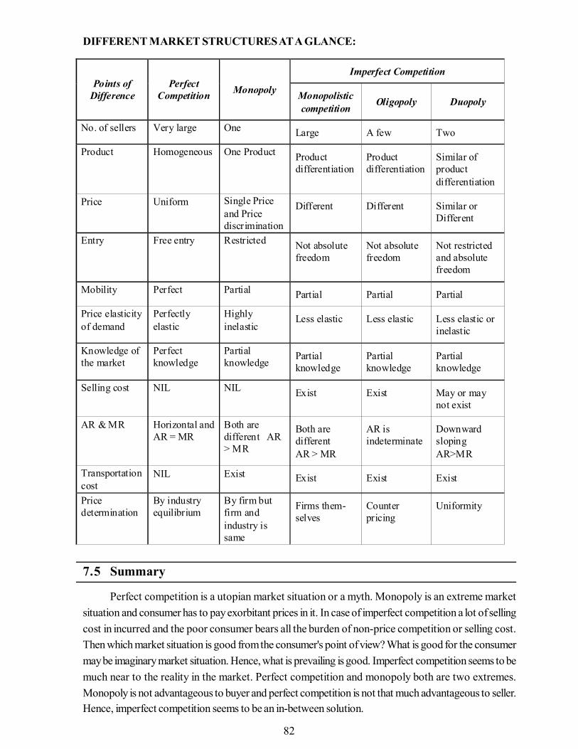
82

DIFFERENT MARKET STRUCTURES AT A GLANCE:

7.5 Summary

Perfect competition is a utopian market situation or a myth. Monopoly is an extreme marketsituation and consumer has to pay exorbitant prices in it. In case of imperfect competition a lot of sellingcost in incurred and the poor consumer bears all the burden of non-price competition or selling cost.Then which market situation is good from the consumer's point of view? What is good for the consumermay be imaginary market situation. Hence, what is prevailing is good. Imperfect competition seems to bemuch near to the reality in the market. Perfect competition and monopoly both are two extremes.Monopoly is not advantageous to buyer and perfect competition is not that much advantageous to seller.Hence, imperfect competition seems to be an in-between solution.

Points of Difference

Perfect Competition Monopoly

Imperfect Competition

Monopolistic competition Oligopoly Duopoly

No. of sellers Very large One Large A few Two

Product Homogeneous One Product Product differentiation

Product differentiation

Similar of product differentiation

Price Uniform Single Price and Price discrimination

Different Different Similar or Different

Entry Free entry Restricted Not absolute freedom

Not absolute freedom

Not restricted and absolute freedom

Mobility Perfect Partial Partial Partial Partial

Price elasticity of demand

Perfectly elastic

Highly inelastic

Less elastic Less elastic Less elastic or inelastic

Knowledge of the market

Perfect knowledge

Partial knowledge

Partial knowledge

Partial knowledge

Partial knowledge

Selling cost NIL NIL Exist Exist May or may not exist

AR & MR Horizontal and AR = MR

Both are different AR > MR

Both are different AR > MR

AR is indeterminate

Downward sloping AR>MR

Transportation cost

NIL Exist Exist Exist Exist

Price determination

By industry equilibrium

By firm but firm and industry is same

Firms themselves

Counter pricing

Uniformity

83

7.6 Key Words

• Market: A place where buyers & sellers are actively engaged in buying and selling acts.

• Market Structure: Market structure is called characteristics of market.

• Perfect Competition: It is characterized by the presence of many firms and they all sell identicalproduct, the seller is a price taker not price maker.

• Monopoly: Market structure, which there is only a single seller of the product.

• Imperfect Market: Here many seller of the product but the product of each seller is differentfrom other seller.

• Monopolistic Competition: It is the mid-way between perfect competition & monopoly.

• Oligopoly: In this market structure, there are a few sellers of a product selling identical ordifferentiated products.

• Duopoly: Only two firms in a market having complete hold over the supply of the product.

7.6 Self Assesment Test

1. Define Market.

2. What are the essentials of a market?

3. Give the characteristics of Perfect Competition.

4. What is Monopoly and what are its characteristics?

5. What is imperfect competition and its forms?

6. What are the characteristics of Monopolistic competition?

7. What is oligopoly and what are its characteristics?

8. Compare Oligopoly and Monopoly.

7.8 Suggeted Books/References

1. Gupta, E.S. : Managerial Economics, Tata MC Grow Hill, New Delhi

2. Dholakiya R.H. and A.H. Ojha: Micro Economics for Management students, Oxford UniversityPress, Delhi.

84

Unit - 8 Pricing Under Different Market ConditionsUnit Structure

8.0 Objectives8.1 Introduction8.2 Objective of Price Output Decision8.3 Price Output Decisions Under Perfect Competition8.4 Price and Output Decisions under Monopoly8.5 Price and Output Decisions under Monopolistic Condition8.6 Pricing and Output Decisionsunder Oligopoly8.7 Summary8.8 Key Words8.9 Self Assessment Test8.10 Suggested Books / References

8.0 Objectives

After studying this unit, you should be able to understand:-

• The concept of market• The objective of price output decision• Price output under Perfect Competition• Price and output under Monopoly• Price and output under monopolistic condition• Pricing and output under Oligopoly

8.1 Introduction

Market:- In general, market means a place where there are many buyers and sellers of differentproducts who are actively engaged in buying and selling acts. The firm's demand curve is expected todepend on such things as the number of sellers in the market and the similarity of their products. These arethe aspects of market structure which may be termed as the characteristics of market of generalisation thatare likely to influence firm's behaviour and performance. In broader sense face to face contact betweenbuyers and sellers is not necessary. They can establish contact through different means of communicationlike letters, agents, telegraphs, telephone etc. or newspapers. Thus, the term market does not mean anyparticular place but the entire area where buyers and sellers of a commodity are in such close contact witheach other that the price of the same commodity tends to be one throughout that area.

The market environment is a marketing term and refers to all of the forces outside marketing thataffect marketing management's ability to build and maintain successful relationships with target customers.The market environment consists of both the macroenvironment and the microenvironment.

The microenvironment refers to the forces that are close to the company and affect its ability toserve its customers. It includes the company itself, its suppliers, marketing intermediaries, customermarkets, competitors, and public.

The company aspect of microenvironment refers to the internal environment of the company. Thisincludes all departments, such as management, finance, research and development, purchasing,operations

85

and accounting. Each of these departments has an impact on marketing decisions. For example, researchand development have input as to the features a product can perform and accounting approves the finan-cial side of marketing plans and budgets.

The suppliers of a company are also an important aspect of the microenvironment because even theslightest delay in receiving supplies can result in customer dissatisfaction. Marketing managers must watchsupply availability and other trends dealing with suppliers to ensure that the product will be delivered tocustomers in the time frame required in order to maintain a strong customer relationship.

8.2 Objective of Price Output Decision

• In decision-making analysis, market structure and pricing has an important role through its impacton the decision-making environment.

• Pricing and market structure is important because it affects market outcomes through its impacton the motivations, opportunities and decisions of economic actors participating in the market.

• The goal of economic market structure and pricing analysis is to isolate these effects in an attemptto explain and predict market outcomes.

• There is close relationship between the price and demand of product.

• Pricing must take into account the competitive and legal environment in which the company operates.

8.3 Price Output Decisions Under Perfect Competition

Perfect competition is a market situation where there are large number of buyers and sellers of ahomogeneous product and the price of the product is determined by the market forces in an industry. Onlysingle price prevails in the market and all the time products are sold at the prevailing price.

PRICE AND OUTPUT DETERMINATION UNDER SHORT PERIOD:

A firm is said to be in equilibrium in short period where marginal cost (MC) is equal to marginalrevenue (MR) and the curve MC cuts MR from below. This also determines the level of output. A shortperiod is the period in which all factors of production cannot be changed, only variable factors like labour,raw material etc. can be changed for the change in the level of output. Hence, short period is such a periodin which no firm enters or leaves an industry.

Under equilibrium position, a firm in short period can have the following situations:

(1) Super Normal profit or Profit situation.(2) Normal profit situation.(3) Loss situation.(4) A case of shut down point.

(1) Super normal profit or a profit situation: As depicted in the diagram 8.1 average revenue (AR) isequal to marginal revenue (MR) which is shown by horizontal line parallel to the x-axis and short runaverage cost (SAC) and short run marginal cost (SMC) have also been shown in the diagram.

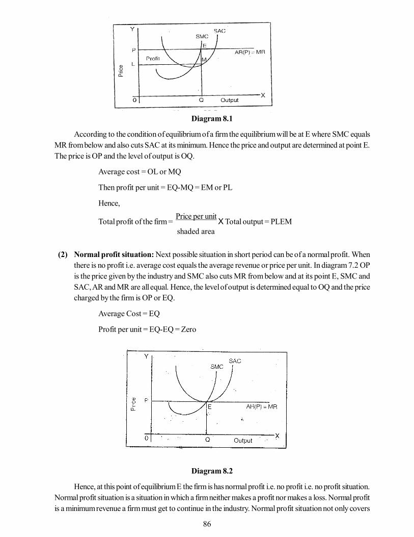
86

Diagram 8.1

According to the condition of equilibrium of a firm the equilibrium will be at E where SMC equalsMR from below and also cuts SAC at its minimum. Hence the price and output are determined at point E.The price is OP and the level of output is OQ.

Average cost = OL or MQ

Then profit per unit = EQ-MQ = EM or PL

Hence,

Total profit of the firm = Price per unit

X Total output = PLEM shaded area

(2) Normal profit situation: Next possible situation in short period can be of a normal profit. Whenthere is no profit i.e. average cost equals the average revenue or price per unit. In diagram 7.2 OPis the price given by the industry and SMC also cuts MR from below and at its point E, SMC andSAC, AR and MR are all equal. Hence, the level of output is determined equal to OQ and the pricecharged by the firm is OP or EQ.

Average Cost = EQ

Profit per unit = EQ-EQ = Zero

Diagram 8.2

Hence, at this point of equilibrium E the firm is has normal profit i.e. no profit i.e. no profit situation.Normal profit situation is a situation in which a firm neither makes a profit nor makes a loss. Normal profitis a minimum revenue a firm must get to continue in the industry. Normal profit situation not only covers

87

explicit cost but also covers the implicit cost of production i.e. cost of owners own resources engaged inproduction.

(3) Loss situation: Third possibility in short period under perfect competition may be of a loss situa-tion where the prevailing market price may be less than the average cost of the firm that is to say thatAR is less than its MC. In such situation the firm will be incurring losses which is well depicted inDiagram 8.3

Diagram 8.3

Here in equilibrium at a point E and output is determined equal to OQ and OP is the price chargedby the firm. At point E, SMC cuts MR from below and SAC at its minimum.

Per unit price = OP or EQ

Per unit cost = OL or MQ

Per unit Loss = ME (=MQ-EQ)

Hence, total loss = LP ME is shown by the shaded area. Under loss situation all the firms will incurlosses and many firms will try to make exit from the industry but due to short period they will be unable todo so. But at the equilibrium position E the firms will be incurring minimum losses.

(4) A case of shut down point: The position is very much clear that in a short period situation the firmcan neither enter can exit. Now the question arises whether the firms will continue production orbreak away, the answer is that the firm will continue production up to a particular level if it is able tomeet its variable cost of production but if AR is less than its average variable cost (AVC) then it willclose its doors and stop production this is well depicted as in diagram 8.4

Diagram 8.4

It is also further elaborated that when the price falls so much that the firm is not able to meet even itsvariable cost then it is advisable to stop the production in the short period. The shut down point arises atthat point where the price is below the variable cost. Thus, in short period when the price is less than thevariable cost then it will stop production. When the price is OP then the level of output is OQ and firm is

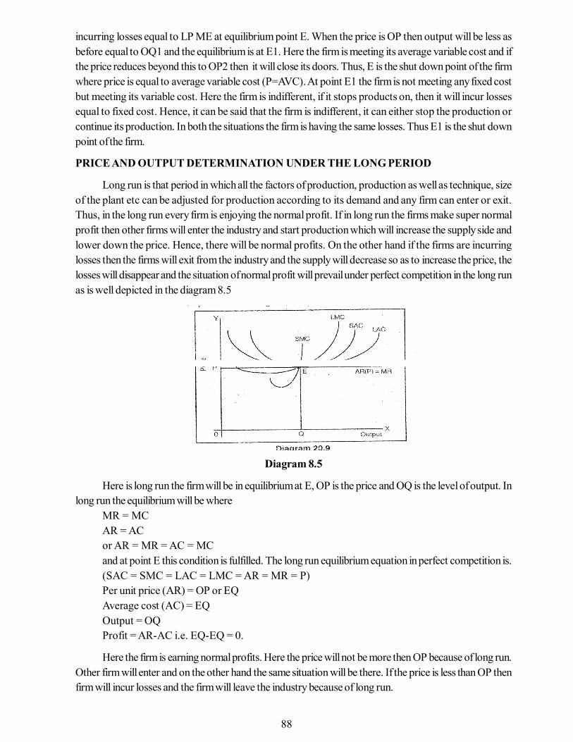
88

incurring losses equal to LP ME at equilibrium point E. When the price is OP then output will be less asbefore equal to OQ1 and the equilibrium is at E1. Here the firm is meeting its average variable cost and ifthe price reduces beyond this to OP2 then it will close its doors. Thus, E is the shut down point of the firmwhere price is equal to average variable cost (P=AVC). At point E1 the firm is not meeting any fixed costbut meeting its variable cost. Here the firm is indifferent, if it stops products on, then it will incur lossesequal to fixed cost. Hence, it can be said that the firm is indifferent, it can either stop the production orcontinue its production. In both the situations the firm is having the same losses. Thus E1 is the shut downpoint of the firm.

PRICE AND OUTPUT DETERMINATION UNDER THE LONG PERIOD

Long run is that period in which all the factors of production, production as well as technique, sizeof the plant etc can be adjusted for production according to its demand and any firm can enter or exit.Thus, in the long run every firm is enjoying the normal profit. If in long run the firms make super normalprofit then other firms will enter the industry and start production which will increase the supply side andlower down the price. Hence, there will be normal profits. On the other hand if the firms are incurringlosses then the firms will exit from the industry and the supply will decrease so as to increase the price, thelosses will disappear and the situation of normal profit will prevail under perfect competition in the long runas is well depicted in the diagram 8.5

Diagram 8.5

Here is long run the firm will be in equilibrium at E, OP is the price and OQ is the level of output. Inlong run the equilibrium will be where

MR = MCAR = ACor AR = MR = AC = MCand at point E this condition is fulfilled. The long run equilibrium equation in perfect competition is.(SAC = SMC = LAC = LMC = AR = MR = P)Per unit price (AR) = OP or EQAverage cost (AC) = EQOutput = OQProfit = AR-AC i.e. EQ-EQ = 0.

Here the firm is earning normal profits. Here the price will not be more then OP because of long run.Other firm will enter and on the other hand the same situation will be there. If the price is less than OP thenfirm will incur losses and the firm will leave the industry because of long run.

89

8.4 Price and Output Decisions Under Monopoly

Monopoly is such a market structure in which there is a single seller of the product. Pure monopolyrefers to a firm producing products which have no close substitutes, which is a rare phenomenon. For themonopoly to exist it is necessary to have producer of the product with no close substitutes of the productsbut there are strong barriers to entry into the industry. In monopoly there is no difference between firm andindustry. Firm and industry is the same which always faces a negatively sloped demand curve for itsproducts. Hence, the monopolist is a price maker not a price-taker. Monopoly therefore, refers to thatmarket in which a single firm controls the whole supply of a particular product which has no close substi-tutes.

PRICE AND OUTPUT DETERMINATION UNDER SHORT PERIOD

Under monopoly market structure a monopolist can make a change in the level of production withmaking a change in scale of production or with intensive use of the productive technique keeping in viewthe time factor which enables the monopolist to do this, is called short period. If a monopolist has toproduce more he can employ more of labour and can change in quantity of raw material and powerresources as required by him. In short period a monopolist cannot influence the fixed costs but variablecosts can only be influenced in the matters of taking decision regarding value and production. Amonopolist in short period cannot charge price less than the average variable cost (AVC) and if he chargesthen he will have to close the door of his firm. Thus a monopolist will remain producing until his marginalcost (MC) equals his marginal revenue (MR) and on this point he enjoys maximum profits. Under shortperiod a monopolist may have super normal profit, normal profits or the losses which is discussed asunder.

A case of super-normal profit under short period: Diagram 8.6 shows the short period equilibriumof the firm where the monopolist has maximum of the profits. In diagram AR and MR are the AverageRevenue and Marginal Revenue curves of the firm and AC and MC are in Average cost and Marginal costcurves of the firm. The firm's MC curve cuts MR curves at point E and establishes equilibrium at point E.At this point the firm's output is OQ and the price is equal to OP and OR or QM is the average cost of thefirm. The difference of OP and OR shows profit equal to PR (per unit profit). Thus, PR MT the shadedarea represents the supernormal profit of a monopolist under short period.

Diagram 8.6A case of normal profit under short period: Under monopoly market a firm may have normal profit

situation which is well illustrated in the diagram 8.7

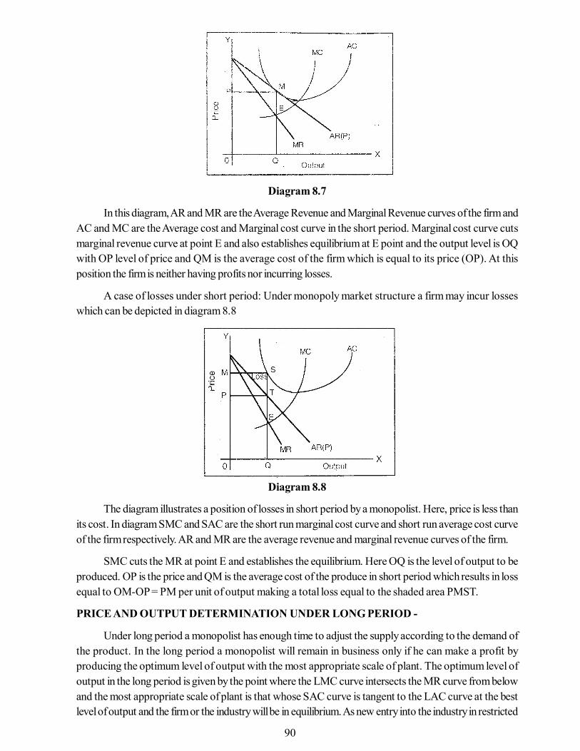
90

Diagram 8.7

In this diagram, AR and MR are the Average Revenue and Marginal Revenue curves of the firm andAC and MC are the Average cost and Marginal cost curve in the short period. Marginal cost curve cutsmarginal revenue curve at point E and also establishes equilibrium at E point and the output level is OQwith OP level of price and QM is the average cost of the firm which is equal to its price (OP). At thisposition the firm is neither having profits nor incurring losses.

A case of losses under short period: Under monopoly market structure a firm may incur losseswhich can be depicted in diagram 8.8

Diagram 8.8

The diagram illustrates a position of losses in short period by a monopolist. Here, price is less thanits cost. In diagram SMC and SAC are the short run marginal cost curve and short run average cost curveof the firm respectively. AR and MR are the average revenue and marginal revenue curves of the firm.

SMC cuts the MR at point E and establishes the equilibrium. Here OQ is the level of output to beproduced. OP is the price and QM is the average cost of the produce in short period which results in lossequal to OM-OP = PM per unit of output making a total loss equal to the shaded area PMST.

PRICE AND OUTPUT DETERMINATION UNDER LONG PERIOD -

Under long period a monopolist has enough time to adjust the supply according to the demand ofthe product. In the long period a monopolist will remain in business only if he can make a profit byproducing the optimum level of output with the most appropriate scale of plant. The optimum level ofoutput in the long period is given by the point where the LMC curve intersects the MR curve from belowand the most appropriate scale of plant is that whose SAC curve is tangent to the LAC curve at the bestlevel of output and the firm or the industry will be in equilibrium. As new entry into the industry in restricted

91

and the firm is the industry as well, the monopolist will adjust the long run output by means of size of plantadjustment depending upon the level and slope of the AR and MR curves.

Diagram 8.9

In the long run the firm will be in equilibrium where firm's LMC curve cuts the long run MR curveand at this point of intersection the firm will enjoy profits. Generally, the firm in the long period is earningsuper-normal profit as shown by diagram 8.9

In the diagram the firm at point E is in equilibrium where LMC cuts MR from below. Thus, E is theequilibrium point where OQ is the output and OP is the price and OM is the average cost of the firm (OM= PQ), hence, the firm is having profit equal to shaded area MPSR. This is a case of profit in long runsituation.

8.5 Price and Output Decisions Under Monopolistic Condition

Monopolistic competition is a situation of imperfect competition. In the previous chapters we havediscussed the perfect competition and monopoly. Both the situations are exceptions to the market struc-ture and the former is imaginary and not found in the real world.

PRICE AND OUTPUT DETERMINATION OF A FRIM UNDER MONOPOLISTICCOMPETITION : A CASE OF SHORT PRIOD EQUILIBRIUM:

The analysis of short period equilibrium of a firm under monopolistic competition is based on thefollowing assumptions:

(1) Large number of sellers who behave independently.

(2) Product of each seller is different (i.e. product differentiation).

(3) The firm has determinate demand curve (AR) which is elastic.

(4) No new firms enter the industry in short period situation.

(5) Short run cost curves of each firms differ from the other.

(6) Factor services are in perfectly elastic supply.

Given these assumptions, each firm fixes such price and output as maximizes its profit. Theequilibrium price and output is determined at a point where the short period marginal cost equals marginalrevenue. Since the cost differs in short period, a firm can earn normal profits, super normal profit or incurlosses. This analysis can be very well depicted in the following diagram 8.10

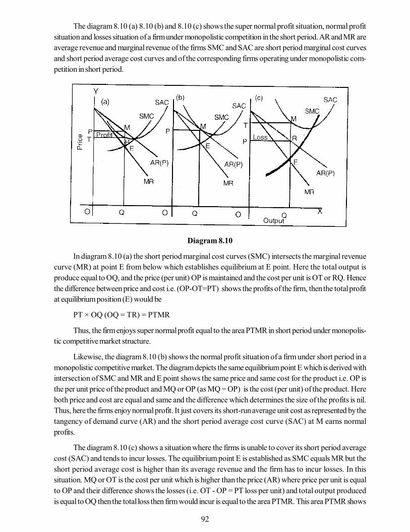
92

The diagram 8.10 (a) 8.10 (b) and 8.10 (c) shows the super normal profit situation, normal profitsituation and losses situation of a firm under monopolistic competition in the short period. AR and MR areaverage revenue and marginal revenue of the firms SMC and SAC are short period marginal cost curvesand short period average cost curves and of the corresponding firms operating under monopolistic com-petition in short period.

Diagram 8.10

In diagram 8.10 (a) the short period marginal cost curves (SMC) intersects the marginal revenuecurve (MR) at point E from below which establishes equilibrium at E point. Here the total output isproduce equal to OQ, and the price (per unit) OP is maintained and the cost per unit is OT or RQ. Hencethe difference between price and cost i.e. (OP-OT=PT) shows the profits of the firm, then the total profitat equilibrium position (E) would be

PT × OQ (OQ = TR) = PTMR

Thus, the firm enjoys super normal profit equal to the area PTMR in short period under monopolis-tic competitive market structure.

Likewise, the diagram 8.10 (b) shows the normal profit situation of a firm under short period in amonopolistic competitive market. The diagram depicts the same equilibrium point E which is derived withintersection of SMC and MR and E point shows the same price and same cost for the product i.e. OP isthe per unit price of the product and MQ or OP (as MQ = OP) is the cost (per unit) of the product. Hereboth price and cost are equal and same and the difference which determines the size of the profits is nil.Thus, here the firms enjoy normal profit. It just covers its short-run average unit cost as represented by thetangency of demand curve (AR) and the short period average cost curve (SAC) at M earns normalprofits.

The diagram 8.10 (c) shows a situation where the firms is unable to cover its short period averagecost (SAC) and tends to incur losses. The equilibrium point E is established as SMC equals MR but theshort period average cost is higher than its average revenue and the firm has to incur losses. In thissituation. MQ or OT is the cost per unit which is higher than the price (AR) where price per unit is equalto OP and their difference shows the losses (i.e. OT - OP = PT loss per unit) and total output producedis equal to OQ then the total loss then firm would incur is equal to the area PTMR. This area PTMR shows

93

the losses of the firm and the firm in short period will continue its production in the hope of lowering downits costs in the long period under monopolistic market structure.

Hence, it should be remembered that in the short period under monopolistic competition theindividual firm may be in equilibrium position but the group as a whole is not in stable equilibrium becausethe number of firms will have a tendency to change. The existence of full equilibrium, for the group is nowhere to be seen in the short period under monopolistic competitive market structure.

PRICE AND OUTPUT DETERMINATION UNDER MONOPOLISTIC COMPETITION: ACASE OF LONG PERIOD EQUILIBRIUM:

In the long period the price and output policy of an individual firm is determined by the one generalprinciple where Marginal revenue (MR) and Marginal cost (MC) are equal to each other as shown in theshort period. The firm can maximise its net profits by equating the long run marginal cost with its marginalrevenue. In long period the individual firm as well as the group as a whole remain in stable equilibriumwhereas in short period the individual firm is in equilibrium but the group is not in stable equilibrium. So, itis possible to achieve the full equilibrium position in the long period under monopolistic competitive marketstructure. To achieve the position of full equilibrium in the long run two adjustments have to be made.

(1) All the quantity offered for sale must be equal to its demand in the market at a given price.

(2) Entry and exit of firms in response to the general position of the existing firm.

The first type of adjustment is similar to that of perfect competition. But under monopolistic compe-tition all the firms do not charge the same price. They charge different prices but the differentials are toomuch. So, under monopolistic competition there is a general level of price and also a general level of AR(Average Revenue) curves of the individual firms. Each firm adjusts its price and output in such a way thatLMC must equal to MR and therefore, each firm determines its output independently. The summation ofthe output of the firms provide us the total output available for sale in the market as shown by diagram8.11. It is assumed here that entry of new firm is restricted.

In diagram 8.11 AR and MR are the average revenue and marginal revenue curve of the firm. LMCand LAC are the long period marginal cost curve and long period average cost curve of the firm. Everyfirm equates its marginal cost to its marginal revenue. In the diagram E1 is the point of equilibrium when theentry of new firms is restricted then the firms enjoying super-normal profits with the OQ level of output asOP is the price and EQ or OM is cost per unit of product and difference between the two shows the profitsituation (i.e. OP-OM = MP) profit per unit and total output is OQ hence, total profit is MP × OQ) equalto the area MPTE. Thus, MPTE is the super-normal profit of a firm under long period situation when theentry of the new firms is restricted but this profit situation will attract other firms to enter.

Diagram 8.11

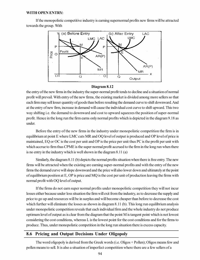
94

WITH OPEN ENTRY:

If the monopolistic competitive industry is earning supernormal profits new firms will be attractedtowards the group. With

Diagram 8.12the entry of the new firms in the industry the super-normal profit tends to decline and a situation of normalprofit will prevail. With entry of the new firms, the existing market is divided among more sellers so thateach firm may sell lesser quantity of goods than before resulting the demand curve to shift downward. Andat the entry of new firm, increase in demand will cause the individual cost curve to shift upward. This twoway shifting i.e. the demand to downward and cost to upward squeezes the position of super-normalprofit. Hence in the long run the firm earns only normal profits which is depicted in the diagram 9.18 asunder.

Before the entry of the new firms in the industry under monopolistic competition the firm is inequilibrium at point E where LMC cuts MR and OQ level of output is produced and OP level of price ismaintained, EQ or OC is the cost per unit and OP is the price per unit thus PC is the profit per unit withwhich accrue to firm thus CPME is the super normal profit accrued to the firm in the long run when thereis no entry in the industry which is well shown in the diagram 8.11 (a)

Similarly, the diagram 8.11 (b) depicts the normal profits situation when there is free entry. The newfirms will be attracted when the existing are earning super-normal profits and with the entry of the newfirms the demand curve will slope downward and the price will also lower down and ultimately at the pointof equilibrium position at E, OP is price and MQ is the cost per unit of production leaving the firms withnormal profit with OQ level of output.

If the firms do not earn super normal profits under monopolistic competition they will not incurlosses either because under loss situation the firm will exit from the industry, as to decrease the supply andprice to go up and resources will be in surplus and will become cheaper than before to decrease the costwhich further will eliminate the losses as shown in diagram 8.11 (b). This long run equilibrium analysisunder monopolistic competition reveals that each individual firm and the whole industry do not produceoptimum level of output as is clear from the diagram that the point M is tangent point which is not lowestconsidering the cost conditions, whereas L is the lowest point for the cost conditions and for the firms toproduce. Thus, under monopolistic competition in the long run situation there is excess capacity.

8.6 Pricing and Output Decisions Under Oligopoly

The word oligopoly is derived from the Greek words (i.e. Oligos + Pollen); Oligos means few andpollen means to sell. It is also a situation of imperfect competition where there are a few sellers of a

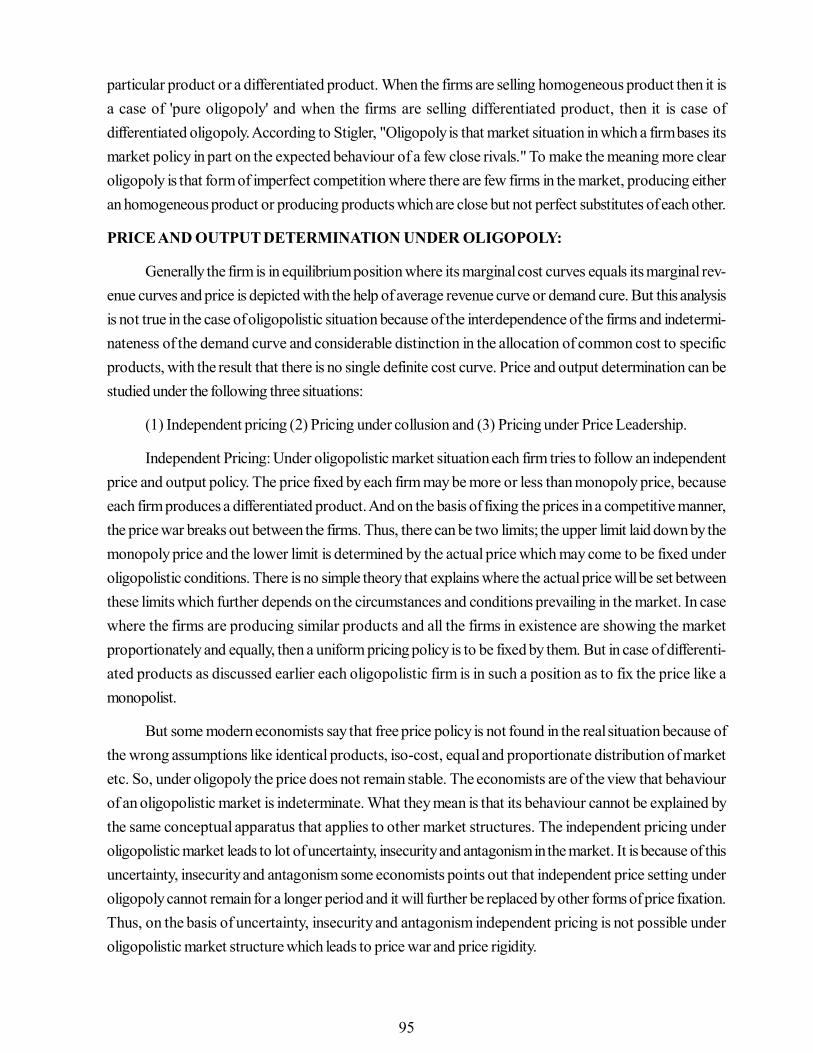
95

particular product or a differentiated product. When the firms are selling homogeneous product then it isa case of 'pure oligopoly' and when the firms are selling differentiated product, then it is case ofdifferentiated oligopoly. According to Stigler, "Oligopoly is that market situation in which a firm bases itsmarket policy in part on the expected behaviour of a few close rivals." To make the meaning more clearoligopoly is that form of imperfect competition where there are few firms in the market, producing eitheran homogeneous product or producing products which are close but not perfect substitutes of each other.

PRICE AND OUTPUT DETERMINATION UNDER OLIGOPOLY:

Generally the firm is in equilibrium position where its marginal cost curves equals its marginal rev-enue curves and price is depicted with the help of average revenue curve or demand cure. But this analysisis not true in the case of oligopolistic situation because of the interdependence of the firms and indetermi-nateness of the demand curve and considerable distinction in the allocation of common cost to specificproducts, with the result that there is no single definite cost curve. Price and output determination can bestudied under the following three situations:

(1) Independent pricing (2) Pricing under collusion and (3) Pricing under Price Leadership.

Independent Pricing: Under oligopolistic market situation each firm tries to follow an independentprice and output policy. The price fixed by each firm may be more or less than monopoly price, becauseeach firm produces a differentiated product. And on the basis of fixing the prices in a competitive manner,the price war breaks out between the firms. Thus, there can be two limits; the upper limit laid down by themonopoly price and the lower limit is determined by the actual price which may come to be fixed underoligopolistic conditions. There is no simple theory that explains where the actual price will be set betweenthese limits which further depends on the circumstances and conditions prevailing in the market. In casewhere the firms are producing similar products and all the firms in existence are showing the marketproportionately and equally, then a uniform pricing policy is to be fixed by them. But in case of differenti-ated products as discussed earlier each oligopolistic firm is in such a position as to fix the price like amonopolist.

But some modern economists say that free price policy is not found in the real situation because ofthe wrong assumptions like identical products, iso-cost, equal and proportionate distribution of marketetc. So, under oligopoly the price does not remain stable. The economists are of the view that behaviourof an oligopolistic market is indeterminate. What they mean is that its behaviour cannot be explained bythe same conceptual apparatus that applies to other market structures. The independent pricing underoligopolistic market leads to lot of uncertainty, insecurity and antagonism in the market. It is because of thisuncertainty, insecurity and antagonism some economists points out that independent price setting underoligopoly cannot remain for a longer period and it will further be replaced by other forms of price fixation.Thus, on the basis of uncertainty, insecurity and antagonism independent pricing is not possible underoligopolistic market structure which leads to price war and price rigidity.

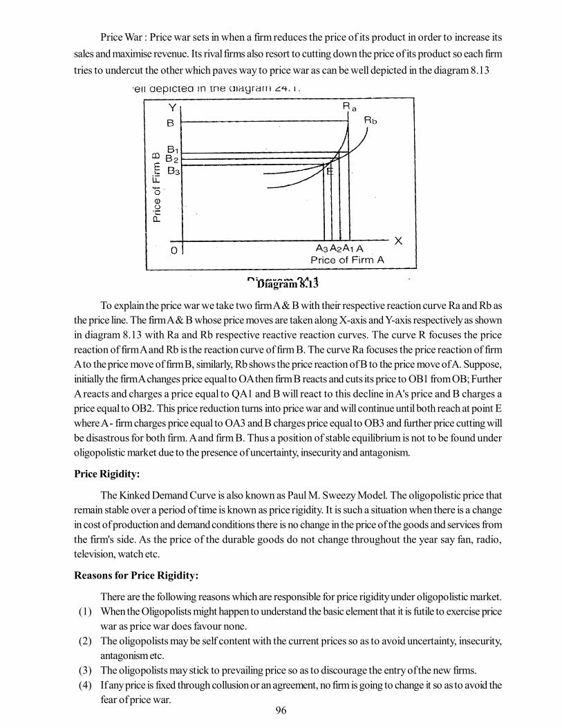
96

Price War : Price war sets in when a firm reduces the price of its product in order to increase itssales and maximise revenue. Its rival firms also resort to cutting down the price of its product so each firmtries to undercut the other which paves way to price war as can be well depicted in the diagram 8.13

Diagram 8.13

To explain the price war we take two firm A & B with their respective reaction curve Ra and Rb asthe price line. The firm A & B whose price moves are taken along X-axis and Y-axis respectively as shownin diagram 8.13 with Ra and Rb respective reactive reaction curves. The curve R focuses the pricereaction of firm A and Rb is the reaction curve of firm B. The curve Ra focuses the price reaction of firmA to the price move of firm B, similarly, Rb shows the price reaction of B to the price move of A. Suppose,initially the firm A changes price equal to OA then firm B reacts and cuts its price to OB1 from OB; FurtherA reacts and charges a price equal to QA1 and B will react to this decline in A's price and B charges aprice equal to OB2. This price reduction turns into price war and will continue until both reach at point Ewhere A - firm charges price equal to OA3 and B charges price equal to OB3 and further price cutting willbe disastrous for both firm. A and firm B. Thus a position of stable equilibrium is not to be found underoligopolistic market due to the presence of uncertainty, insecurity and antagonism.

Price Rigidity:

The Kinked Demand Curve is also known as Paul M. Sweezy Model. The oligopolistic price thatremain stable over a period of time is known as price rigidity. It is such a situation when there is a changein cost of production and demand conditions there is no change in the price of the goods and services fromthe firm's side. As the price of the durable goods do not change throughout the year say fan, radio,television, watch etc.

Reasons for Price Rigidity:

There are the following reasons which are responsible for price rigidity under oligopolistic market. (1) When the Oligopolists might happen to understand the basic element that it is futile to exercise price

war as price war does favour none. (2) The oligopolists may be self content with the current prices so as to avoid uncertainty, insecurity,

antagonism etc. (3) The oligopolists may stick to prevailing price so as to discourage the entry of the new firms. (4) If any price is fixed through collusion or an agreement, no firm is going to change it so as to avoid the

fear of price war.

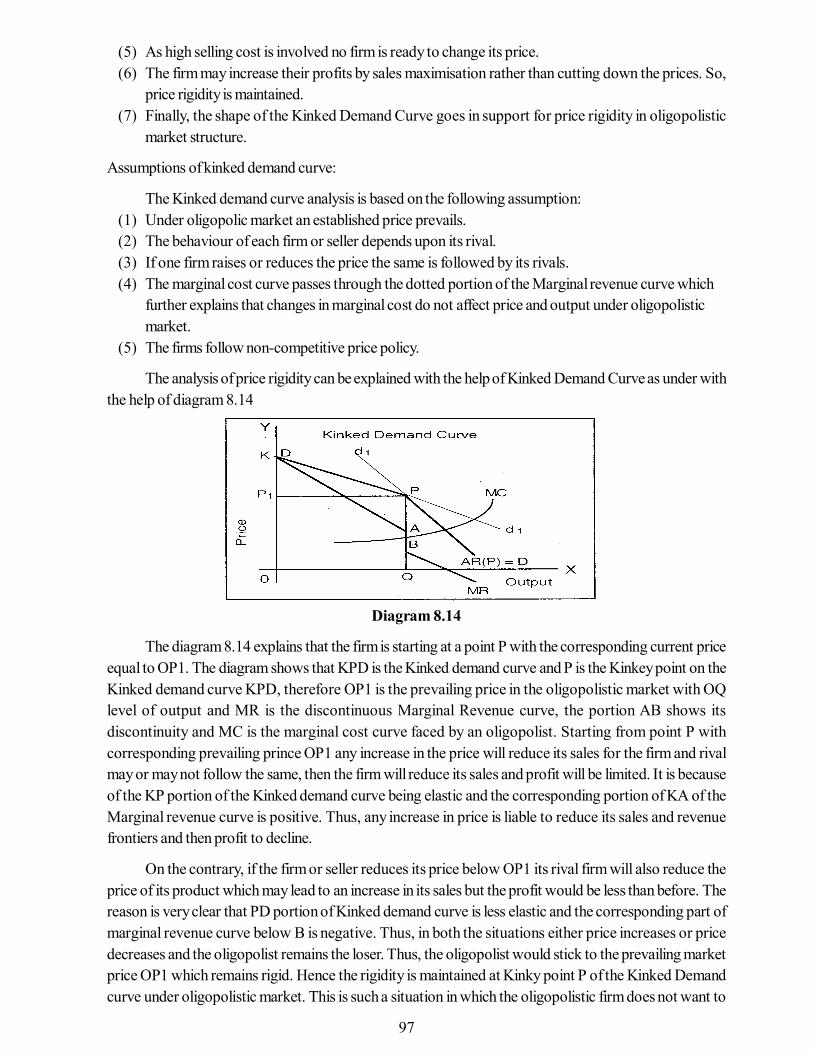
97

(5) As high selling cost is involved no firm is ready to change its price. (6) The firm may increase their profits by sales maximisation rather than cutting down the prices. So,

price rigidity is maintained. (7) Finally, the shape of the Kinked Demand Curve goes in support for price rigidity in oligopolistic

market structure.

Assumptions of kinked demand curve:

The Kinked demand curve analysis is based on the following assumption: (1) Under oligopolic market an established price prevails. (2) The behaviour of each firm or seller depends upon its rival. (3) If one firm raises or reduces the price the same is followed by its rivals. (4) The marginal cost curve passes through the dotted portion of the Marginal revenue curve which

further explains that changes in marginal cost do not affect price and output under oligopolisticmarket.

(5) The firms follow non-competitive price policy.

The analysis of price rigidity can be explained with the help of Kinked Demand Curve as under withthe help of diagram 8.14

Diagram 8.14

The diagram 8.14 explains that the firm is starting at a point P with the corresponding current priceequal to OP1. The diagram shows that KPD is the Kinked demand curve and P is the Kinkey point on theKinked demand curve KPD, therefore OP1 is the prevailing price in the oligopolistic market with OQlevel of output and MR is the discontinuous Marginal Revenue curve, the portion AB shows itsdiscontinuity and MC is the marginal cost curve faced by an oligopolist. Starting from point P withcorresponding prevailing prince OP1 any increase in the price will reduce its sales for the firm and rivalmay or may not follow the same, then the firm will reduce its sales and profit will be limited. It is becauseof the KP portion of the Kinked demand curve being elastic and the corresponding portion of KA of theMarginal revenue curve is positive. Thus, any increase in price is liable to reduce its sales and revenuefrontiers and then profit to decline.

On the contrary, if the firm or seller reduces its price below OP1 its rival firm will also reduce theprice of its product which may lead to an increase in its sales but the profit would be less than before. Thereason is very clear that PD portion of Kinked demand curve is less elastic and the corresponding part ofmarginal revenue curve below B is negative. Thus, in both the situations either price increases or pricedecreases and the oligopolist remains the loser. Thus, the oligopolist would stick to the prevailing marketprice OP1 which remains rigid. Hence the rigidity is maintained at Kinky point P of the Kinked Demandcurve under oligopolistic market. This is such a situation in which the oligopolistic firm does not want to

98

have a change in its price, maintaining rigidity at the Kinky point of the Kinked demand curve. Thus pricerigidity is always maintained at the Kinky point on the Kinked demand curve under oligopolistic market.The demand curve KPD with P as Kinky point on it presents a discontinuity in marginal revenue curveequal to the portion AB and beyond B the marginal revenue curve is negative. The elasticity of Kinkeddemand curve determines the size of discontinuity in the marginal revenue curve. The more elastic thedemand curve is to the left of the Kinky point P and more inelastic to right of the Kinky point, the more willbe discontinuity in the marginal revenue curve under oligopolistic market in the price rigidity analysis. If theangle, KPD becomes a right angle the gap or discontinuity (AB) will be the widest. Thus, the price will bestable and rigid till marginal cost curve cuts marginal revenue curve, somewhere between the discontinuityportion AB. The Theory of Kinked demand curve has its drawbacks.

(i) The gap or discontinuity or Marginal Revenue Curve (MR) may be unstable.

(ii) The theory does not tell us how the initial price OP1 is maintained.

(iii) Price determination is illusionary as it does not follow the market behaviour.

(iv) It is doubtful about the stability of price under oligopoly as actual sales price in case of manyproducts is not possible.

(v) Kinked theory follows a price cut but does not follow a price rise but Stigler remarked that a pricerise has not been taken into consideration.

PERFECT COLLUSION UNDER OLIGOPOLY:

A collusion or a cartel is a combination of firms whose object is to limit the scope of competitiveforces within a market. Individual firms of a certain industry surrender to a central association the powerto make price and output decisions. Thus, the cartel or collusive oligopoly assumes monopoly power thedetermines the price and output in the same capacity with zeal and jest. Perfect collusion implies cartelagreements which is an association of the independent firms within the industry. Perfect cartel underoligopoly with complete control over the price and output policy of the member firms and with the threatof entry is a situation for consideration.

(1) Perfect collusion: Perfect cartel is an extreme form of perfect collusion. Each firm reserves profitsaccording to the assigned quota and therefore the principle of cost maximisation is not likely to befollowed. Thus, it is also contemplated that price and output results obtained under perfect collusiveoligopoly are the same as obtained under monopoly. The price and output under central can be illustratedwith the help of following diagram 8.15.

Diagram 8.15

99

In diagram 8.14 DD is the industry demand curve and MR is the corresponding marginal revenuecurve taking three oligopolistic firms A, B and C in the industry. Their marginal cost curves are MC1,MC2 and MC3 respectively with OP1 level of price with their respective output equal to OQ1m OQ2and OQ3. MC is the lateral summation of the marginal cost curves of all the individual firm in the industrywhich equals Marginal revenue curve at point E with OQ level of output with the price level OP, as DD isthe demand curve for the industry and also determines the price for the industry as a whole under theconditions of perfect collusion and each firm will produce that level of output at which marginal cost curvesequals industry's marginal revenue curves i.e. EP1. Thus A will produce OQ1, B will produce OQ2 and Cwill produce OQ3 of the output and OQ being the total output of the industry (OQ1+OQ2+OQ3 = OQ).It results into the maximum joint profit for the industry but it is not necessary that each firm may have profitequal to their quota allotment. Mutual agreement and relative bargaining power determine the division ofprofit.

(2) Market Sharing Cartel under Oligopoly:

Another form of perfect collusion under oligopolistic market is that of market sharing cartel by themember firms of a cartel. Market sharing cartel is an equal division of total market sales among all its firms.In differentiated oligopoly all firms in an industry enter into a collusion for charging a uniform price whichis agreeable to all the firms. They divide the market among themselves according to an agreement and getprofits according to its sales and their demand curve will be a part of the demand curve for the industry. Aseach firm has its own demand curve with the same elasticity as that of industry demand curve which can beillustrated in diagram 8.16

When equal market's sharing DD is the industry demand curve and MR is the corresponding mar-ginal revenue curve (DD1) MC is the aggregate marginal cost curve of the industry. MR curve DD1intersects MC curve at point E and set OP price and OQ level of output under this situation. Industryoutput OQ is shared equally by the firms at MC curve of firms cuts MR curve at point C and OQ level ofoutput is determined as OQ level of output is for the industry as a whole. Thus, OQ is just half of the totaloutput QO or OQ0 - QoQ level of output. Thus, equal level of output is shared by the firms. Each firmtries to increase the share of the market by means of secret price concessions which tends to change thedemand cost conditions further and price variations among firms become more common and ultimately theagreement becomes a farce and all the firms act independent oligopolists.

Diagram 8.16

100

PRICE LEADERSHIP:

Price leadership is imperfect collusion among the oligopolistic firms in an industry with the dominantfirm as all firms follow the dominant firm as one of the big firm in an oligopolistic market. There is anagreement among all the firms to sell the product at a price set by the leader of the dominant firm in anindustry. Sometimes a meeting is held and a definite agreement is taken by the dominant firm. In case ofhomogeneous or heterogeneous product the price may be a uniform price and the same is announced bythe leader of the firms for example, price leadership industries are like cement, cigarettes, flour, fertilizers,petroleum, milk, steel, etc. Price leadership may be of different types. (i) There is a barometric price in which there is no dominant firm which announces the price but the

wisest firm announces the price by taking into consideration the demand and cost conditions andthe rest follow suit.

(ii) When the price is announced by a dominant firm then it is known as dominant price leadership. It isalso known as partial monopolistic price leadership.

(iii) The dominating firm may fix the profit maximisation price for itself and for the others to accept it; itis known as aggressive price leadership. It may fix such a low price as some of the firms may resortto exit from the industry.

(iv) When the pricing is done by the dominant firm suppressing competition among oligopoly firms isknown as effective price leadership.

The real test of the dominant firms price leadership is the extent to which the other firms follow itslead. The moment the firms cease to follow the price leader, the model of price leadership by the dominantfirm seems to break down. Besides, if the other firms have different cost curves the same price may notmaximise short run profits for all the firms under oligopolistic situation under the head of price leadership.

The price leadership firm may keep in mind the following points while exercising price leadership:

1- The reactions of the firms when the price is announced. 2- Elasticity of substitution between the product of the price leadership firm and the competitive firms. 3- Knowledge about the policy of the competitive firms.

The price determination by the price leadership firm can be illustrated with the help of the diagram8.17

Diagram 8.17

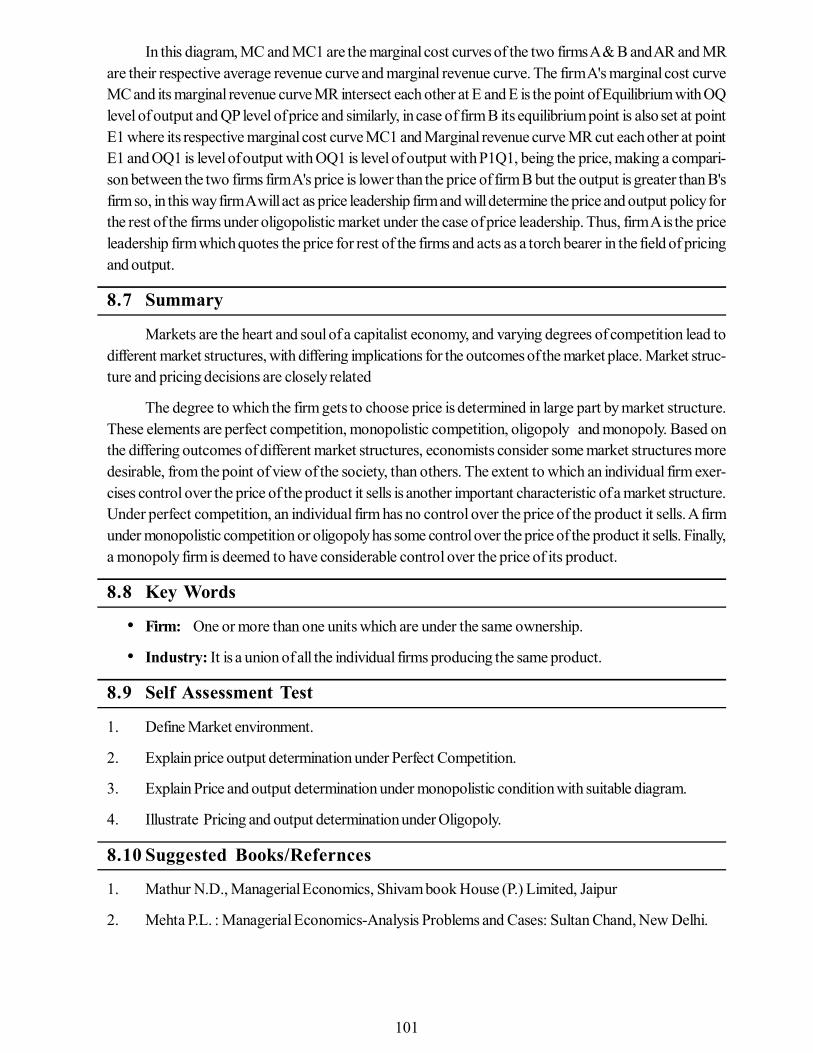
101

In this diagram, MC and MC1 are the marginal cost curves of the two firms A & B and AR and MRare their respective average revenue curve and marginal revenue curve. The firm A's marginal cost curveMC and its marginal revenue curve MR intersect each other at E and E is the point of Equilibrium with OQlevel of output and QP level of price and similarly, in case of firm B its equilibrium point is also set at pointE1 where its respective marginal cost curve MC1 and Marginal revenue curve MR cut each other at pointE1 and OQ1 is level of output with OQ1 is level of output with P1Q1, being the price, making a compari-son between the two firms firm A's price is lower than the price of firm B but the output is greater than B'sfirm so, in this way firm A will act as price leadership firm and will determine the price and output policy forthe rest of the firms under oligopolistic market under the case of price leadership. Thus, firm A is the priceleadership firm which quotes the price for rest of the firms and acts as a torch bearer in the field of pricingand output.

8.7 Summary

Markets are the heart and soul of a capitalist economy, and varying degrees of competition lead todifferent market structures, with differing implications for the outcomes of the market place. Market struc-ture and pricing decisions are closely related

The degree to which the firm gets to choose price is determined in large part by market structure.These elements are perfect competition, monopolistic competition, oligopoly and monopoly. Based onthe differing outcomes of different market structures, economists consider some market structures moredesirable, from the point of view of the society, than others. The extent to which an individual firm exer-cises control over the price of the product it sells is another important characteristic of a market structure.Under perfect competition, an individual firm has no control over the price of the product it sells. A firmunder monopolistic competition or oligopoly has some control over the price of the product it sells. Finally,a monopoly firm is deemed to have considerable control over the price of its product.

8.8 Key Words

• Firm: One or more than one units which are under the same ownership.

• Industry: It is a union of all the individual firms producing the same product.


1. Define Market environment.

2. Explain price output determination under Perfect Competition.

3. Explain Price and output determination under monopolistic condition with suitable diagram.

4. Illustrate Pricing and output determination under Oligopoly.

8.10 Suggested Books/Refernces

1. Mathur N.D., Managerial Economics, Shivam book House (P.) Limited, Jaipur

2. Mehta P.L. : Managerial Economics-Analysis Problems and Cases: Sultan Chand, New Delhi.

102

Unit - 9 Price DiscriminationUnit Structure

9.0 Objectives9.1 Introduction9.2 Objectives of Price Discrimination9.3 Conditions necessary for Price Discrimination to Work9.4 Types of Price Discrimination9.5 International Price Discrimination: Dumping9.6 Disadvantages of Price Discrimination9.7 Price Discrimination-harmful or Beneficial to Society9.8 Summary9.9 Key Words9.10 Self Assessment Test9.11 Suggested Books / References

9.0 Objectives


• The concept of price discrimination• The objectives of price discrimination• Types of price discrimination• The concept of dumping• Price Discrimination-harmful or beneficial to society

9.1 Introduction

Price discrimination or price differentiation exists when sales of identical goods or services aretransacted at different prices from the same provider. In a theoretical market with perfect information,perfect substitutes, and no transaction costs or prohibition on secondary exchange (or re-selling) toprevent arbitrage, price discrimination can only be a feature of monopolistic and oligopolistic markets,where market power can be exercised. Otherwise, the moment the seller tries to sell the same goods atdifferent prices, the buyer at the lower price can arbitrage by selling to the consumer buying at the higherprice but with a small discount. However, product heterogeneity, market frictions or high fixed costs(which make marginal-cost pricing unsustainable in the long run) can allow for some degree of differentialpricing to different consumers, even in fully competitive retail or industrial markets. Price discriminationalso occurs when the same price is charged from customers which have different supply costs.

Difference between price discrimination and product differentiationProduct differentiation differentiation of the product gives the supplier greater control over price

and the potential to charge consumers a premium price because of actual or perceived differences in thequality / performance of goods or services.

Price discrimination occurs when a firm charges a different price from different groups ofconsumers for an identical good or service, for reasons not associated with costs.

9.2 Objectives of Price Discrimination

There are several objectives of price discrimination. Some are as given below.

103

• Firms will be able to increase revenue. This will enable some firms to stay in business whichotherwise would have made a loss. For example price discrimination is important for traincompanies which offer different prices for peak and off peak.

• Increased revenues can be used for research and development which benefit consumers

• Some consumers will benefit from lower fares. Eg. old people benefit from lower train companies,old people are more likely to be poor

• The other objective to the consumer of price discrimination are - price discrimination is likely toincrease output and make the good or service available to more people and the increasedcompetition in the market leads to lower prices and more choice.

9.3 Conditions Necessary for Price Discrimination to Work

Essentially there are two main conditions required for discriminatory pricing

1) Differences in price elasticity of demand between markets: There must be a different price elasticityof demand from each group of consumers. The firm is then able to charge a higher price from thegroup with a more price inelastic demand and a relatively lower price from the group with a moreelastic demand. By adopting such a strategy, the firm can increase its total revenue and profits (i.e.achieve a higher level of producer surplus). To profit maximize, profit the firm will seek to setmarginal revenue equal to marginal cost in each separate (segmented) market.

2) Barriers to prevent consumers switching from one supplier to another: The firm must be able toprevent "market seepage" or "consumer switching" - defined as a process whereby consumers whohave purchased goods or services at a lower price are able to re-sell it to those consumers whowould have normally paid the expensive price. This can be done in a number of ways, - and isprobably easier to achieve with the provision of a unique service such as a haircut rather than withthe exchange of tangible goods. Seepage might be prevented by selling a product to consumers atunique and different points in time - for example with the use of time specific airline tickets thatcannot be resold under any circumstances.

The effects of price discrimination on social efficiency are unclear; typically such behavior leads tolower prices for some consumers and higher prices for others. Output can be expanded when pricediscrimination is very efficient, but output can also decline when discrimination is more effective atextracting surplus from high-valued users than expanding sales to low valued users. Even if output remainsconstant, price discrimination can reduce efficiency by misallocating output among consumers.

9.4 Types of Price Discrimination

There are many forms of price discrimination, but the standard method of classification identifiesthree types or degrees of discrimination. But there are other two types also named as skimming andcombination. Their common characteristic is that they allow the firm to capture part of the consumersurplus that would have resulted from uniform pricing.

First degree price discrimination

In first degree price discrimination, price varies by customer's willingness or ability to pay. Thisarises from the fact that the value of goods is subjective. A customer with low price elasticity is lessdeterred by a higher price than a customer with high price elasticity of demand. As long as the price

104

elasticity (in absolute value) for a customer is less than one, it is very advantageous to increase the price:the seller gets more money for fewer goods. With an increase of the price elasticity tends to rise aboveone. One can show that in optimum price, as it varies from customer to cuustomer, is inverselyproportional to one minus the reciprocal of the price elasticity of that customer at that price. This assumesthat the consumer passively reacts to the price set by the seller, and that the seller knows the demandcurve of the customer. In practice however there is a bargaining situation, which is more complex: thecustomer may try to influence the price, such as by pretending to like the product less than he or she reallydoes or by threatening not to buy it.

An alternative way to understand first Degree Price Discrimination is as follows: This type of pricediscrimination is primarily theoretical because it requires the seller of goods or services to know theabsolute maximum price that every consumer is willing to pay. As above, it is true that consumers havedifferent price elasticities, but the seller is not concerned with thus. The seller is concerned with themaximum willingness to pay (or reservation price) of each customer. By knowing the reservation price, theseller is able to absorb the entire market surplus, thus taking all of the consumer's surplus from theconsumer and transforming it into revenues. From a social welfare perspective though, first degree pricediscrimination is not necessarily undesirable. That is, the market is still entirely efficient and there is nodeadweight loss to society. In a market with first degree price discrimination, the seller simply captures allsurplus. Efficiency is unchanged but the wealth is transferred. This type of market does not exist much inreality, hence it is primarily theoretical. Examples of where this might be observed are in markets whereconsumers bid for tenders, though still, in this case, the practice of collusive tendering underminesefficiency. It is a classic part of price competition between firms seeking a market advantage or to protectan established market position.

Perfect Price Discrimination - charging whatever the market will bear

Sometimes known as optimal pricing, with perfect price discrimination, the firm separates the wholemarket into each individual consumer and charges them the price they are willing and are able to pay. Ifsuccessful, the firm can extract all consumer surplus that lies beneath the demand curve and turn it intoextra producer revenue (or producer surplus). This is impossible to achieve unless the firm knows everyconsumer's preferences and, as a result, is unlikely to occur in the real world. The transactions costsinvolved in finding out through market research what each buyer is prepared to pay is the main block orbarrier to a businesses engaged in this form of price discrimination.

If the monopolist is able to perfectly segment the market, then the average revenue curve effectivelybecomes the marginal revenue curve for the firm. The monopolist will continue to see extra units as long asthe extra revenue exceeds the marginal cost of production.

The reality is that, although optimal pricing can and does take place in the real world, most suppliersand consumers prefer to work with price lists and price menus from which trade can take place rather thanhaving to negotiate a price for each unit of a product bought and sold.

105

Diagram 9.1

Diagram 9.1 shows the demand curve faced by a monopolist. The curve indicates the maximumprice that can be obtained for successive units of output. For example, the first unit Q1, could commanda maximum price of P1, the second could be sold for a maximum of P2, and so on. To simplify thediscussion, it is assumed that marginal cost is constant and equal to average cost.

First-degree discrimination involves charging the maximum price possible for each unit of output.Thus, the consumer who attaches the greatest value to the product is identified and charged a price of P1.Similarly, the consumers willing to pay P2 for the second unit and P3 for the third are identified andrequired to pay P2 and P3, respectively.

With first-degree price discrimination, the profit-maximizing output rate is where the marginal costand demand curves intersect. In Figure 9.1, it occurs at QD. At this point, the maximum price that can beobtained for the product is just equal to the marginal cost of production. Any attempt to sell more than QDunits would reduce profits because price would have to be less than marginal cost. Conversely, any rate ofoutput less than QD would not maximize profits because the additional units could be sold (as shown bythe demand curve) at prices greater than the marginal cost.

First-degree discrimination is the most extreme form of price discrimination and the most profitablepricing scheme for the firm. Because buyers are charged the maximum price for each unit of output, noconsumer surplus remains. Consumer surplus is the difference between the price a consumer is willing topay and the actual price charged for the good or service. The maximum consumer surplus results whenthere is no price discrimination, and price is set equal to marginal cost. In Fig 9.1, this maximum consumersurplus is shown as the area of the triangle APcB. In contrast with first-degree price discrimination, thereis no consumer surplus because APcB is captured by the firm as economic profit.

Second degree price discrimination

In second degree price discrimination, price varies according to quantity sold. Larger quantities areavailable at a lower unit price. This is particularly widespread in sales to industrial customers, where bulkbuyers enjoy higher discounts.

Additionally to second degree price discrimination, sellers are not able to differentiate betweendifferent types of consumers. Thus, the suppliers will provide incentives for the consumers to differentiatethemselves according to preference. As above, quantity "discounts", or non-linear pricing, is a means bywhich suppliers use consumer preference to distinguish classes of consumers. This allows the supplier to

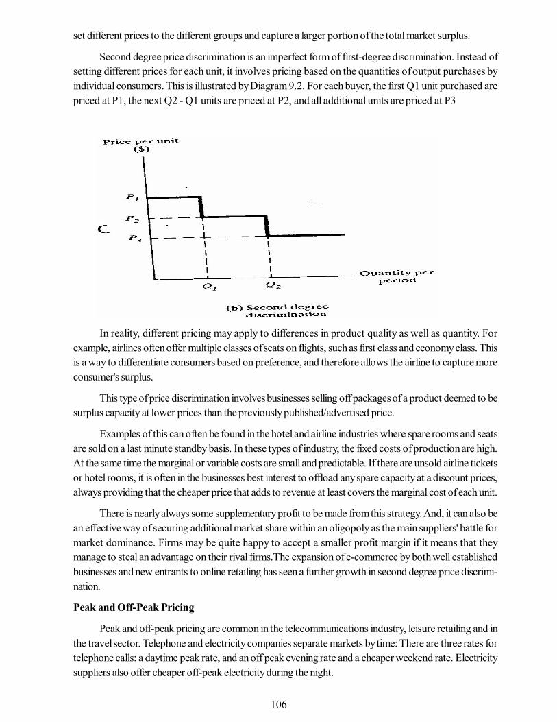
106

set different prices to the different groups and capture a larger portion of the total market surplus.

Second degree price discrimination is an imperfect form of first-degree discrimination. Instead ofsetting different prices for each unit, it involves pricing based on the quantities of output purchases byindividual consumers. This is illustrated by Diagram 9.2. For each buyer, the first Q1 unit purchased arepriced at P1, the next Q2 - Q1 units are priced at P2, and all additional units are priced at P3

Diagram10.2

In reality, different pricing may apply to differences in product quality as well as quantity. Forexample, airlines often offer multiple classes of seats on flights, such as first class and economy class. Thisis a way to differentiate consumers based on preference, and therefore allows the airline to capture moreconsumer's surplus.

This type of price discrimination involves businesses selling off packages of a product deemed to besurplus capacity at lower prices than the previously published/advertised price.

Examples of this can often be found in the hotel and airline industries where spare rooms and seatsare sold on a last minute standby basis. In these types of industry, the fixed costs of production are high.At the same time the marginal or variable costs are small and predictable. If there are unsold airline ticketsor hotel rooms, it is often in the businesses best interest to offload any spare capacity at a discount prices,always providing that the cheaper price that adds to revenue at least covers the marginal cost of each unit.

There is nearly always some supplementary profit to be made from this strategy. And, it can also bean effective way of securing additional market share within an oligopoly as the main suppliers' battle formarket dominance. Firms may be quite happy to accept a smaller profit margin if it means that theymanage to steal an advantage on their rival firms.The expansion of e-commerce by both well establishedbusinesses and new entrants to online retailing has seen a further growth in second degree price discrimi-nation.

Peak and Off-Peak Pricing

Peak and off-peak pricing are common in the telecommunications industry, leisure retailing and inthe travel sector. Telephone and electricity companies separate markets by time: There are three rates fortelephone calls: a daytime peak rate, and an off peak evening rate and a cheaper weekend rate. Electricitysuppliers also offer cheaper off-peak electricity during the night.

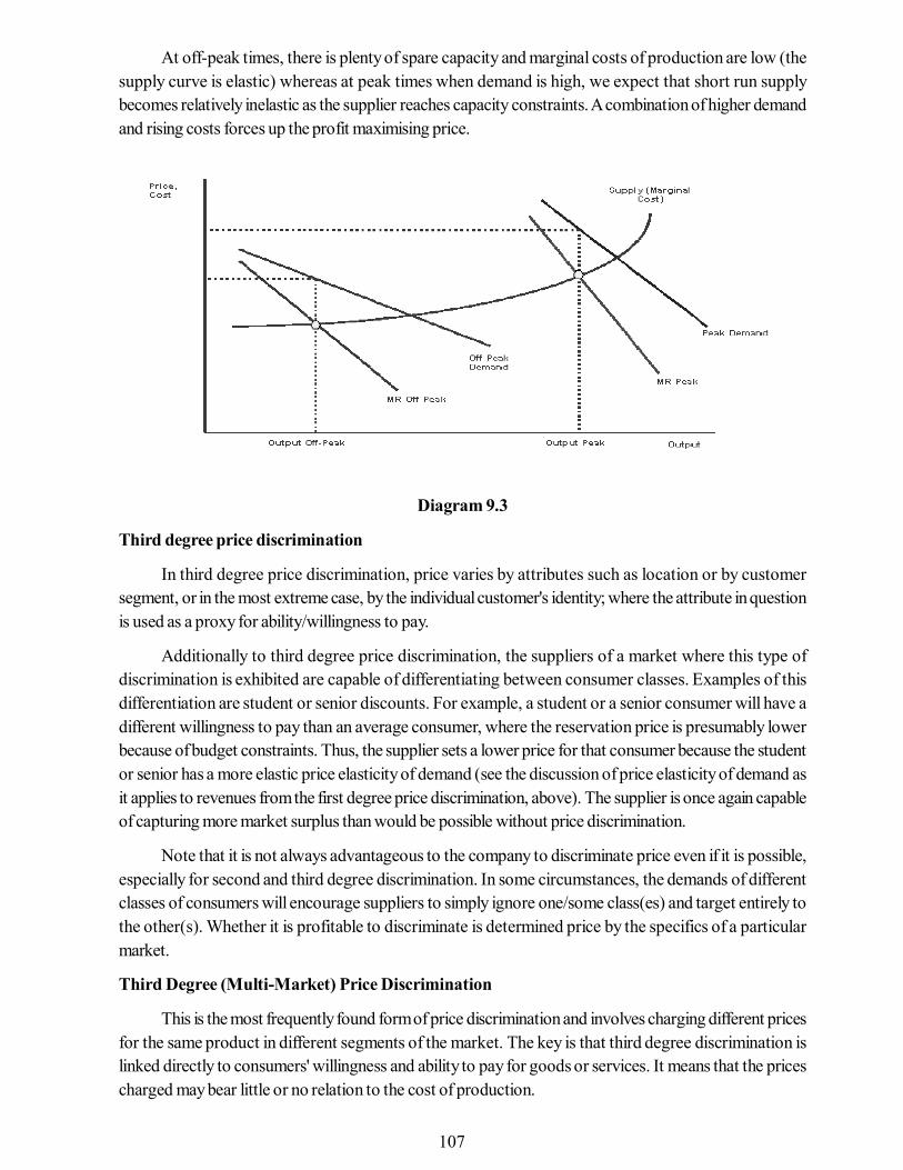
107

At off-peak times, there is plenty of spare capacity and marginal costs of production are low (thesupply curve is elastic) whereas at peak times when demand is high, we expect that short run supplybecomes relatively inelastic as the supplier reaches capacity constraints. A combination of higher demandand rising costs forces up the profit maximising price.

Diagram 9.3

Third degree price discrimination

In third degree price discrimination, price varies by attributes such as location or by customersegment, or in the most extreme case, by the individual customer's identity; where the attribute in questionis used as a proxy for ability/willingness to pay.

Additionally to third degree price discrimination, the suppliers of a market where this type ofdiscrimination is exhibited are capable of differentiating between consumer classes. Examples of thisdifferentiation are student or senior discounts. For example, a student or a senior consumer will have adifferent willingness to pay than an average consumer, where the reservation price is presumably lowerbecause of budget constraints. Thus, the supplier sets a lower price for that consumer because the studentor senior has a more elastic price elasticity of demand (see the discussion of price elasticity of demand asit applies to revenues from the first degree price discrimination, above). The supplier is once again capableof capturing more market surplus than would be possible without price discrimination.

Note that it is not always advantageous to the company to discriminate price even if it is possible,especially for second and third degree discrimination. In some circumstances, the demands of differentclasses of consumers will encourage suppliers to simply ignore one/some class(es) and target entirely tothe other(s). Whether it is profitable to discriminate is determined price by the specifics of a particularmarket.

Third Degree (Multi-Market) Price Discrimination

This is the most frequently found form of price discrimination and involves charging different pricesfor the same product in different segments of the market. The key is that third degree discrimination islinked directly to consumers' willingness and ability to pay for goods or services. It means that the pricescharged may bear little or no relation to the cost of production.

108

The market is usually separated in two ways: by time or by geography. For example, exporters maycharge a higher price in overseas markets if demand is estimated to be more inelastic than it is in homemarkets. MC=AC

Diagram 9.4

Suppose a firm has separated a market by time into a peak market with inelastic demand, and anoff-peak market with elastic demand. The demand and marginal revenue curves for the peak market andoff peak markets are labelled A and B respectively. This is illustrated in the diagram above. Assuming aconstant marginal cost for supplying to each group of consumers, the firm aims to charge a profit maximisingprice to each group.

In the peak market the firm will produce where MRa = MC and charge price Pa, and in theoff-peak market the firm will produce where MRb = MC and charge price Pb. Consumers with aninelastic demand for the product will pay a higher price (Pa) than those with an elastic demand who will becharged Pb.

Price Skimming

In price skimming, price varies over time. Typically a company starts selling a new product at arelatively high price then gradually reduces the price as the low price elasticity segment gets satiated. Priceskimming is closely related to the concept of yield management. Price skimming is a pricing strategy inwhich a marketer sets a relatively high price for a product or service at first, then lowers the price overtime. It is a temporal version of price discrimination/yield management. It allows the firm to recover itssunk costs quickly before competition steps in and lowers the market price.

Diagram 9.5

109

Price skimming is sometimes referred to as riding down the demand curve. The objective of a priceskimming strategy is to capture the consumer surplus. If this is done successfully, then theoretically nocustomer will pay less for the product than the maximum they are willing to pay. In practice, it is almostimpossible for a firm to capture all of this surplus.

Combination

These types are not mutually exclusive. Thus a company may vary pricing by location, but then offerbulk discounts as well. Airlines use several different types of price discrimination, including:

• Bulk discounts to wholesalers, consolidators, and tour operators • Incentive discounts for higher sales volumes to travel agents and corporate buyers • Seasonal discounts, incentive discounts, and even general prices that vary by location. The price of

a flight from say, Singapore to Beijing can vary widely if one buys the ticket in Singapore comparedto Beijing (or New York or Tokyo or elsewhere). In online ticket sales this is achieved by using thecustomer's credit card billing address to determine his location.

• Discounted tickets requiring advance purchase and/or Saturday stays. Both restrictions have theeffect of excluding business travelers, who typically travel during the workweek and arrange tripson shorter notice.

• First degree price discrimination based on customer. It is not accidental that hotel or car rental firmsmay quote higher prices to their loyalty program's top tier members than to the general public

9.5 International Price Discrimination: Dumping

In economics, "dumping" can refer to any kind of predatory pricing. However, the word is nowgenerally used only in the context of international trade law, where dumping is defined as the act of amanufacturer in one country exporting a product to another country at a price which is either below theprice it charges in its home market or is below its costs of production. The term has a negativeconnotation, but advocates of free markets see "dumping" as beneficial for consumers and believe thatprotectionism to prevent it would have net negative consequences. Advocates for workers and laborershowever, believe that safeguarding businesses against predatory practices, such as dumping, help alleviatesome of the harsher consequences of free trade between economies at different stages of development(see protectionism). The Bolkestein directive, for example, was accused in Europe of being a form of"social dumping," as it favored competition between workers, as exemplified by the Polish Plumberstereotype. While there are very few examples of a national scale dumping that succeeded in producing anational-level monopoly, there are several examples of dumping that produced a monopoly in regionalmarkets for certain industries. Ron Chenow points to the example of regional oil monopolies in Titan : TheLife of John D. Rockefeller, Sr. where Rockefeller receives a message from Colonel Thompson outliningan approved strategy where oil in one market, Cincinnati, would be sold at or below cost to drivecompetition's profits down and force them to exit the market. In another area where other independentbusinesses were already driven out, namely in Chicago, prices would be increased by a quarter.

A standard technical definition of dumping is the act of charging a lower price for a good in a foreignmarket than one charges for the same good in a domestic market. This is often referred to as selling at lessthan "fair value". Under the World Trade Organization (WTO) Agreement, dumping is condemned (but isnot prohibited) if it causes or threatens to cause material injury to a domestic industry in the importingcountry.

110

Remedies and penalties

In the United States, domestic firms can file an antidumping petition under the regulationsdetermined by the United States Department of Commerce, which determines "less than fair value" andthe International Trade Commission, which determines "injury". These proceedings operate on a timetablegoverned by U.S. law. The Department of Commerce has regularly found that products have been sold atless than fair value in U.S. markets. If the domestic industry is able to establish that it is being injured by thedumping, then antidumping duties are imposed on goods imported from the dumpers' country at a per-centage rate calculated to counteract the dumping margin.

Related to antidumping duties are "countervailing duties". The difference is that countervailing dutiesseek to offset injurious subsidization while antidumping duties offset injurious dumping.

Some commentators have noted that domestic protectionism, and lack of knowledge regardingforeign cost of production, lead to the unpredictable institutional process surrounding investigation. Mem-bers of the WTO can file complaints against anti-dumping measures.

Legal issues

If a company exports a product at a price lower than the price it normally charges on its own homemarket, it is said to be "dumping" the product. Opinions differ as to whether or not this is unfair competi-tion, but many governments take action against dumping in order to defend their domestic industries. TheWTO agreement does not pass judgment. Its focus is on how governments can or cannot react to dump-ing-it disciplines anti-dumping actions, and it is often called the "Anti-Dumping Agreement". (This focusesonly on the reaction to dumping contrasts with the approach of the Subsidies & Countervailing MeasuresAgreement.)

The legal definitions are more precise, but broadly speaking the WTO agreement allows govern-ments to act against dumping where there is genuine ("material") injury to the competing domestic industry.In order to do that the government has to be able to show that dumping is taking place, calculate the extentof dumping (how much lower the export price is compared to the exporter's home market price), andshow that the dumping is causing injury or threatening to do so.

Definitions and degrees of dumping

While permitted by the WTO, General Agreement on Tariffs and Trade (GATT) (Article VI) allowscountries the option of taking action against dumping. The Anti-Dumping Agreement clarifies and expandsArticle VI, and the two operate together. They allow countries to act in a way that would normally breakthe GATT principles of binding a tariff and not discriminating between trading partners-typically anti-dumping action means charging extra import duty on the particular product from the particular exportingcountry in order to bring its price closer to the "normal value" or to remove the injury to domestic industryin the importing country.

There are many different ways of calculating whether a particular product is being dumped heavilyor only lightly. The agreement narrows down the range of possible options. It provides three methods tocalculate a product's "normal value". The main one is based on the price in the exporter's domestic mar-ket. When this cannot be used, two alternatives are available-the price charged by the exporter in anothercountry, or a calculation based on the combination of the exporter's production costs, other expenses andnormal profit margins. And the agreement also specifies how a fair comparison can be made between theexport price and what would be a normal price.

111

Calculating the extent of dumping on a product is not enough. Anti-dumping measures can only beapplied if the dumping is hurting the industry in the importing country. Therefore, a detailed investigationhas to be conducted according to specified rules first. The investigation must evaluate all relevanteconomic factors that have a bearing on the state of the industry in question. If the investigation showsdumping is taking place and domestic industry is being hurt, the exporting company can undertake to raiseits price to an agreed level in order to avoid anti-dumping import duty.

Procedures in investigation and litigation

Detailed procedures are set out on how anti-dumping cases are to be initiated, how theinvestigations are to be conducted, and the conditions for ensuring that all interested parties are given anopportunity to present evidence. Anti-dumping measures must expire five years after the date ofimposition, unless a review shows that ending the measure would lead to injury.

Anti-dumping investigations are to end immediately in cases where the authorities determine that themargin of dumping is, de minimis, or insignificantly small (defined as less than 2% of the export price of theproduct). Other conditions are also set. For example, the investigations also have to end if the volume ofdumped imports is negligible (i.e., if the volume from one country is less than 3% of total imports of thatproduct-although investigations can proceed if several countries, each supplying less than 3% of the im-ports, together account for 7% or more of total imports). The agreement says member countries mustinform the Committee on Anti-Dumping Practices about all preliminary and final anti-dumping actions,promptly and in detail. They must also report on all investigations twice a year. When differences arise,members are encouraged to consult each other. They can also use the WTO's dispute settlement proce-dure.

9.6 Disadvantages of Price Discrimination 1. Some consumers will end up paying higher prices. These higher prices are likely to be allocatively

inefficient because P>MC. 2. Decline in consumer surplus. 3. Those who pay higher prices may not be the poorest. 4. There may be administration costs in separating the markets. 5. Profits from price discrimination could be used to finance predatory pricing.

9.7 Price Discrimination-Harmful or Beneficial to Society

Pigou and Joan Robinson have analyzed the circumstances under which price discrimination isharmful or beneficial to society. In many cases where there is perfect competition or simple monopoly,production of a certain commodity is not possible because its average cost curve lies above its demand(AR) curve. But under price discrimination, the average cost curve is likely to be below the averagerevenue curve at some point. Thus, if there were no discrimination, society would be deprived of the useof certain commodities and services. As emphasized by Mrs Robinson: "It may happen, for instance, thata railway would not be built, or a country doctor would not set up practice, if discrimination wereforbidden. From the point of view of society, it is only necessary that the concern should make sufficientprofits to maintain the efficiency of the plant, and not a profit which would have been sufficient to justifythe original investment." If a doctor charges a uniform fee from all his patients, his income may be so lowas to induce him to leave his private practice and join some hospital. The community is thus deprived of hisservices in that particular area where he is practicing. If, however, he charges more fee from his richpatients than from the ordinary, his income is likely to be so high as to induce him from stay in that area.

112

Similarly, the existence of railways depends upon their charging higher rates to some customers than fromothers.

If discrimination occurs under conditions of falling average costs, it is actually beneficial to consum-ers because it results in larger output for the market. This is illustrated in Figure 4 where D is the averagerevenue curve of the discriminating monopolist and d/MR is the ordinary demand curve which becomesthe MR curve to the discriminator. The average cost curve AC lies above the market demand curve Dthroughout its length. So no production is possible at any price on the D curve. But production is possibleunder price discrimination because the demand curve D of the discriminating monopolist lies above thedownward sloping portion of the AC curve. Equilibrium is established at E where MC = MR and theoutput OQ is produced and sold at QP price and the discriminator earns RP profits per unit of output.

Diagram 9.6

Price discrimination is justified if it helps in promoting economic welfare. Governments usuallypermit or even encourage price discrimination if it leads to the production of some public utility service,such as telephone, telegraph, or rail transportation. In public utility services, the higher income groups arecharged higher prices and the funds so collected may be used to subsidies the goods meant for the poor.

Price discrimination is also beneficial to society for it helps in reducing inequalities of personalincomes when higher prices or fees are charged from the rich than from the poor. In public utility services,the higher price charged from the higher income groups serves as a tool for income redistribution becausethe government may use these funds to subsidies the lower income groups. Thus price discrimination helpsin promoting social welfare.

Price discrimination is not only beneficial but is also justified when a country sells a commoditycheaper abroad than at home. If a foreign market is elastic, more will be sold at a lower price. It meansexpansion in output, the use of larger resources of the economy, more employment and income to thecommunity. Price discrimination of this type proves particularly useful if the industry obeys the law ofdecreasing costs. It implies the realization of larger economies of scale, lowering of costs and prices to thehome market also. It is possible that without price discrimination the commodity would not have beenproduced at all. In that case, had it been imported from abroad, it would have cost the economy moreboth in monetary and real terms. Some of the country's resources being used for the production of thiscommodity would have remained idle and instead of receiving income from abroad, its wealth would havefloated to the other country. May be, economies of scale could be realized only when the monopoliststarted producing for the foreign market. Hence price discrimination is justified.

113

Price discrimination is, however, harmful to society when it leads to a misdistribution of resources asbetween different uses with the result that output, employment and income are not maximized. Further, itmay lead to the diversion of resources from their socially optimal uses. It leads to wastes of resourceswhen people are made to pay higher prices for smaller quantities. Even on international plane when pricediscrimination takes the form of dumping, it deliberately shatters the economy of the other country byundercutting the foreign producers and forcing them to close their business. Such discrimination is highlyundesirable.

9.8 Summary

Price discrimination is the practice of one retailer, wholesaler, or manufacturer charging differentprices for the same items from different customer. This is a widespread practice. Price discrimination, asit is now understood, is separated into degrees. First, second and third degree price discrimination existand apply to different pricing methods used by companies. Much depends on the understanding of themarket in segments, and also the consumer's ability to pay a higher or lower price, called elasticity ofdemand. A person who might pay more for an item is thought to have a low elasticity of demand. Anotherperson who will not pay as much has a high elasticity of demand.

9.9 Key Words • Price discrimination: Price discrimination exists when sales of identical goods or services are

transacted at different prices from the same provider. In general, the practice of charging differentcustomers different prices is called price discrimination.

• First degree price discrimination: Price discrimination exists when sales of identical goodsor services are transacted at different prices from the same provider. In general, the practice ofcharging different customers different prices is called price discrimination.

• Second degree price discrimination: Price discrimination exists when sales of identical goodsor services are transacted at different prices from the same provider. In general, the practice ofcharging different customers different prices is called price discrimination.

• Third degree price discrimination: Price discrimination exists when sales of identical goodsor services are transacted at different prices from the same provider. In general, the practice ofcharging different customers different prices is called price discrimination.

• Dumping: Selling goods abroad at a price below that charged in the domestic market.


1 What is price discrimination? What are the conditions for discriminating price?

2 What are the objectives of price discrimination?

3 Briefly explain types of price discrimination.

4 What do you think price discrimination-harmful or beneficial to society?

5 What is international price discrimination? Explain its legal issues.


1. Mansfield E.C. : Micro Economics - Selected Reading W.W. Norten, New York

2. Koutsoyiannis A: Reading in applied Economics: Oxford Clarendoor Press.

114

Unit - 10 Pricing StrategiesUnit Structure

10.0 Objectives10.1 Introduction10.2 Objectives of Pricing Strategy10.3 Cost-Plus Pricing10.4 Pricing Over Life-Cycle of a Product10.5 Multiple Product Pricing10.6 Transfer Pricing10.7 Pricing In Relation To Established Products10.8 Peak-load Pricing10.9 Ramsey Pricing10.10 Limit Pricing10.11 Loss Leader Pricing10.12 Summary10.13 Key Words10.14 Self Assessment Test10.15 Suggested Books / References

10.0 Objectives


• The concept of pricing strategy.• Pricing strategies followed by firms in specific situations.• Pricing strategy and their impact on demand.• The objectives of pricing strategy.

10.1 Introduction

In every economics system, the prices of goods and services are crucial. A price is a sacrifice forone who pays it but it is a gain for one who gets it. Everybody is concerned with the prices in one way oranother. The price of the commodity would be determined by the market itself through interplay ofdemand and supply for the commodity, because there is a relationship between price and quantitydemanded, it is important to understand the impact of pricing on sales by estimating the demand curve forthe product. For existing products, experiments can be performed at prices above and below the currentprice in order to determine the price elasticity of demand. Inelastic demand indicates that price increasesmight be feasible.

Pricing strategy las an instrument to achieve the objective of a firm and it should be formulated insuch a way as to maximize the sales revenue and profit. Maximum profit refers to the highest possibleprofit. In the short run, a firm not only should be able to recover its total costs, but also should get excessrevenue over costs.

One of the most difficult, yet important, issues you must decide as an entrepreneur is how much tocharge for your product or service. While there is no one single right way to determine your pricingstrategy, fortunately there are some guidelines that will help you with your decision.

115

10.2 Objectives of Pricing Strategy

The firm's pricing strategy objectives must be identified in order to determine the optimal pricing indifferent market situations. Common objectives include the following:

• Current profit maximization - seeks to maximize current profit, taking into account revenue andcosts. Current profit maximization may not be the best objective if it results in lower long-termprofits.

• Current revenue maximization - seeks to maximize current revenue with no regard to profit margins.The underlying objective often is to maximize long-term profits by increasing market share andlowering costs.

• Maximize quantity - seeks to maximize the number of units sold or the number of customers servedin order to decrease long-term costs as predicted by the experience curve.

• Maximize profit margin - attempts to maximize the unit profit margin, recognizing that quantities willbe low.

• Quality leadership - use price to signal high quality in an attempt to position the product as thequality leader.

• Partial cost recovery - an organization that has other revenue sources may seek only partial costrecovery.

• Survival - in situations such as market decline and overcapacity, the goal may be to select a pricethat will cover costs and permit the firm to remain in the market. In this case, survival may take apriority over profits, so this objective is considered temporary.

• Status quo - the firm may seek price stabilization in order to avoid price wars and maintain amoderate but stable level of profit.

10.3 Cost-Plus Pricing

Cost-plus pricing is also known as 'mark-up pricing', 'average cost pricing' or 'full cost pricing'. Thecost-plus pricing is the most common method of pricing used by the manufacturing firms. It is usedprimarily because it is easy to calculate and requires little information. There are several varieties, but thecommon thread in all of them is you first calculate the cost of the product, and then include an additionalamount to represent profit.

Calculating price using the cost-plus method

There are several ways of determining cost, and the profit can be added as either a percentage markup oran absolute amount. One example is:

P = (AVC + FC%) x (1 + MK%)

Where:

• P = price • AVC = average variable cost • FC% = percentage allocation of fixed costs • MK% = percentage markup

116

For example: If variable costs are 30 yen, the allocation to cover fixed costs is 10 yen, and you feelyou need a 50% markup then you would charge a price of 60 yen:

P = (30 + 10) x (1 + 0.50)

P = 40 x 1.5

P = 60

An alternative way of doing the same calculation is:

P = (AVC + FC%) / (1 ? MK%)

To make things simpler, some firms, particularly retailers, ignore fixed costs and just use thepurchase price paid to their suppliers as the cost term. They indirectly incorporate the fixed cost allocationinto the markup percentage. To simplify things even further, sometimes a fixed amount is applied ratherthan a percentage. This fixed amount is usually determined by head-office to make it easy for franchiseesand store managers. This is sometimes referred to as turnkey pricing.

Another variant of cost plus pricing is activity based pricing. This involves being more careful indetermining costs. Instead of using arbitrary expense categories when allocating overhead, every activityis linked to the resources it uses.

Advantages of cost-plus pricing :-

1. easy to calculate2. minimal information requirements3. easy to administer4. tends to stabilize markets - insulated from demand variations and competitive factors5. ethical advantages

Disadvantages of cost-plus pricing :-

1. tends to ignore the role of consumers2. tends to ignore the role of competitors3. use of historical accounting costs rather than replacement value4. inclusion of sunk costs rather than just using incremental costs5. ignores opportunity costs

10.4 Pricing over Life-Cycle of a Product

Product life cycle management (or PLCM) is the succession of strategies used by businessmanagement as a product goes through its life cycle. The life-cycle of a product is generally divided intofour stages: (i) Introduction (ii) Growth, (iii) Maturity, (iv) Decline. Diagram 11.1presents the four stagesof a product's life-cycle through a curve showing the behavior of the total sales over the life cycle. Theintroduction phase is the period taken to introduce the product to the market. The total sale during thisperiod is limited to the quantity put on the market for trial with considerable advertisement. The salesduring this period remain almost constant. Growth is the stage, after a successful trail, during which theproduct gains popularity among the consumers and sales increase at an increasing rate as a result ofcumulative effect of advertisement over the initial stage. Maturity is the stage in which sales continue toincrease but at a lower rate and the total sale eventually becomes constant. After the maturity stage, comesthe stage of decline in which total sales register a declining trend for such reasons as (i) increase in theavailability of substitutes, and (ii) the loss of distinctiveness of the product.

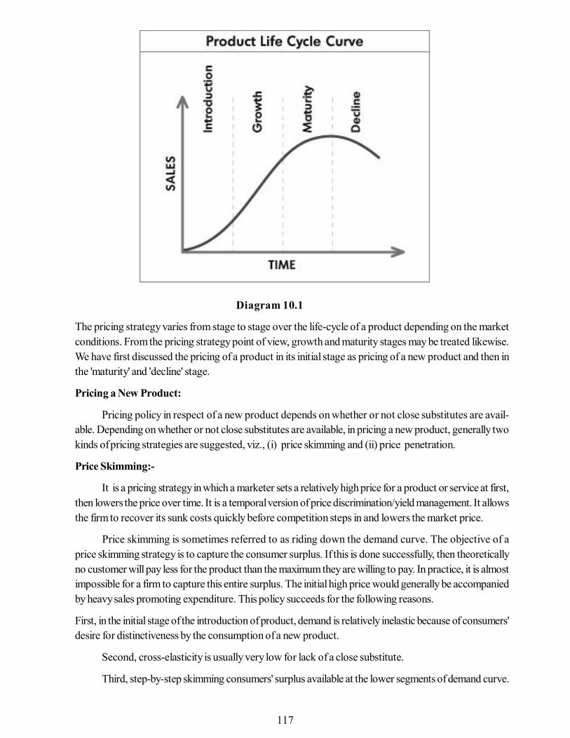
117

Diagram 10.1

The pricing strategy varies from stage to stage over the life-cycle of a product depending on the marketconditions. From the pricing strategy point of view, growth and maturity stages may be treated likewise.We have first discussed the pricing of a product in its initial stage as pricing of a new product and then inthe 'maturity' and 'decline' stage.

Pricing a New Product:

Pricing policy in respect of a new product depends on whether or not close substitutes are avail-able. Depending on whether or not close substitutes are available, in pricing a new product, generally twokinds of pricing strategies are suggested, viz., (i) price skimming and (ii) price penetration.

Price Skimming:-

It is a pricing strategy in which a marketer sets a relatively high price for a product or service at first,then lowers the price over time. It is a temporal version of price discrimination/yield management. It allowsthe firm to recover its sunk costs quickly before competition steps in and lowers the market price.

Price skimming is sometimes referred to as riding down the demand curve. The objective of aprice skimming strategy is to capture the consumer surplus. If this is done successfully, then theoreticallyno customer will pay less for the product than the maximum they are willing to pay. In practice, it is almostimpossible for a firm to capture this entire surplus. The initial high price would generally be accompaniedby heavy sales promoting expenditure. This policy succeeds for the following reasons.

First, in the initial stage of the introduction of product, demand is relatively inelastic because of consumers'desire for distinctiveness by the consumption of a new product.

Second, cross-elasticity is usually very low for lack of a close substitute.

Third, step-by-step skimming consumers' surplus available at the lower segments of demand curve.

118

Penetration Pricing:-It is the pricing technique of setting a relatively low initial entry price, often lower than the eventual

market price, to attract new customers. The strategy works on the expectation that customers will switchto the new brand because of the lower price. Penetration pricing is most commonly associated with amarketing objective of increasing market share or sales volume, rather than to make profit in the shortterm.

The success of penetration price policy requires the existence of the following conditions.

First, the short run demand for the product should have elasticity greater than unity. It helps incapturing the market at lower prices.

Second, economies of large-scale production are available to the firm with the increase in sales.Otherwise, increase in production would result in increase in costs which might reduce the competitive-ness of the price.

Third, the product should have a high cross-elasticity in relation to rival products for the initial lowerprice to be effective.

Finally, the product, by nature should be such that it can be easily accepted and adopted by theconsumers.

Pricing in Maturity Period:

Maturing period is the second stage in the life-cycle of a product. It is a stage between the growthperiod and decline period of sales. Sometimes maturity period is bracketed with saturation period. Matu-rity period may also be defined as the period of decline in the growth rate of sales (not the total sales) andthe period of zero growth rate. The concept of maturity period is useful to the extent it gives out signals fortaking precaution with regard to pricing policy. However, the concept itself does not provide guidelines forthe pricing policy. Joel Dean suggests that the "first step for the manufacturer whose specialty is about toslip into the commodity category is to reduce real...prices as soon as the system of deterioration appears."But he warns that "this does not mean that the manufacturer should declare open price war in the industry".He should rather move in the direction of "product improvement and market segmentation".

Pricing a Product in Decline:

The product in decline is one that enters the post-maturity stage. In this stage, the total sale of theproduct starts declining. The first step in pricing strategy in this stage is obviously to reduce the price. Theproduct should be reformulated and remodeled to suit the consumers' preferences. It is a commonpractice in the book trade. When the sale of a hard-bound edition reaches saturation, paper-back editionis brought into the market. This facility is, however, limited to only a few

10.5 Multiple Product Pricing

The price theory or microeconomic models of price determination are based on the assumption thata firm produces a single, homogeneous product. In actual practice, however, production of a singlehomogeneous product by a firm is an exception rather than a rule. Almost all firms have more than oneproduct in their line of production. Even the most specialized firms produce a commodity in multiplemodels, styles and sizes, each so much differentiated from the other that each model or size of the productmay be considered a different product. For example, the various models of refrigerators, TV sets, radioand car models produced by the same company may be treated as different products for at least pricing

119

purpose. The various models are so differentiated that consumers view them as different products and insome cases, as perfect substitutes for each other. It is, therefore, not surprising that each model or producthas different AR and MR curves and that one product of the firm competes against the other product. Thepricing under these conditions is known as multi-product pricing or product-line pricing.

The major problem in pricing multiple products is that each product has a separate demand curve.But, since all of them are produced under one organization by interchangeable production facilities, theyhave only one inseparable marginal, cost curve. That is, while revenue curves, AR and MR, are separatefor each product, cost curves, AC and MC, are inseparable. Therefore, the marginal rule of pricing cannotbe applied straightaway to fix the price of each product separately. The problem, however, has beenprovided with a solution by E.W. Clements. The solution is similar to the one employed to illustrate thirddegree price discrimination. As a discriminating monopoly tries to maximize its revenue in all its markets,so does a multi-product firm in respect of each of its products.

To illustrate the multiple product pricing, let us suppose that a firm has four different products - A,B, C and D in its line of production. The AR and MR curves for the four goods are shown in four segmentsof Diagram 10.2 The marginal cost for all the products taken together is shown by

Diagram 10.2

The marginal cost for all the products taken together is shown by the curve MC, which is the factorymarginal cost curve. Let us suppose that when the MRs for the individual products are horizontally summedup, the aggregate MR (not given in the figure) passes through point C on the MC curve. If a line parallel tothe X-axis, is drawn from point C to the Y-axis through the MRs, the intersecting points will show thepoints where MC and MRs are equal for each product, as shown by the line EMR, the Equal MarginalRevenue line. The points of intersection between EMR and MRs determine the output level and price foreach product. The output of the four products are given as OQ1 of product A; Q1Q2 of B; Q2Q3 of C;Q3Q4 of D. The respective prices for the four products are: P1Q1 for product A; P2Q2 for B; P3Q3 forC, and P4Q4 for D. These price and output combinations maximize the profit from each product andhence the overall profit of the firm.

120

10.6 Transfer Pricing

Transfer pricing refers to the setting, analysis, documentation, and adjustment of charges madebetween related parties for good, services, or use of property (including intangible property). Transferprices among components of an enterprise may be used to reflect allocation of resources among suchcomponents, or for other purposes. we can say the price at which transfer takes place called transferprice. A high price will increase profits of the units at the earlier stage of production, whereas a low pricewill make later stage production more profitable. while an incorrect price can affect the total profit earnedby the firm.

Transfer Pricing with No External Market

The discussion in this section explains an economic theory behind optimal transfer pricing withoptimal defined as transfer pricing that maximizes overall firm profits in a non-realistic world with no taxes,no capital risk, no development risk, no externalities or any other frictions which exist in the real world. Inpractice a great many factors influence the transfer prices that are used by multinational corporations,including performance measurement, capabilities of accounting systems, import quotas, customs duties,VAT, taxes on profits, and (in many cases) simple lack of attention to the pricing.

Diagram 10.3

From marginal price determination theory, the optimum level of output is that where marginal costequals marginal revenue. That is to say, a firm should expand its output as long as the marginal revenuefrom additional sales is greater than their marginal costs. In the diagram that follows, this intersection isrepresented by point A, which will yield a price of P*, given the demand at point B.

It can be shown algebraically that the intersection of the firm's marginal cost curve and marginalrevenue curve (point A) must occur at the same quantity as the intersection of the production division'smarginal cost curve with the net marginal revenue from production (point C).

Transfer Pricing with a Competitive External Market

When a firm is selling some of its product to itself, and only to itself (i.e. there is no external marketfor that particular transfer good), then the picture gets more complicated, but the outcome remains the

121

same. The demand curve remains the same. The optimum price and quantity remain the same. Butmarginal cost of production can be separated from the firm's total marginal costs. Likewise, the marginalrevenue associated with the production division can be separated from the marginal revenue for the totalfirm. This is referred to as the Net Marginal Revenue in production (NMR) and is calculated as themarginal revenue from the firm minus the marginal costs of distribution.

Diagram 10.4

If the production division is able to sell the transfer good in a competitive market (as well asinternally), then again both must operate where their marginal costs equal their marginal revenue, for profitmaximization. Because the external market is competitive, the firm is a price taker and must accept thetransfer price determined by market forces (their marginal revenue from transfer and demand for transferproducts becomes the transfer price). If the market price is relatively high (as in Ptr1 in the next diagram),then the firm will experience an internal surplus (excess internal supply) equal to the amount Qt1 minusQf1. The actual marginal cost curve is defined by points A,C,D.

Transfer Pricing with an Imperfect External Market

If the firm is able to sell its transfer goods in an imperfect market, then it need not be a price taker.There are two markets each with its own price (Pf and Pt in the next diagram).

Diagram 10.5

122

The aggregate market is constructed from the first two. That is, point C is a horizontal summation ofpoints A and B (and likewise for all other points on the Net Marginal Revenue curve (NMRa)). The totaloptimum quantity (Q) is the sum of Qf plus Qt.

10.7 Pricing for Established Products

In pricing a product in relation to its well established substitutes, generally three types of pricingstrategies are adopted, viz., (i) pricing below the ongoing price, (ii) pricing at par with the prevailingmarket price, and (iii) pricing above the existing market price. Let us now see which of these strategies areadopted under what conditions.

Pricing Below the Market-Price:

Pricing below the prevailing market price of the substitutes is generally preferred under two condi-tions. First, if a firm wants to expand its product-mix with a view to utilizing its unused capacity in the faceof tough competition with the established brands, the strategy of pricing below the market price is gener-ally adopted. This strategy gives the new brand an opportunity to gain popularity and establish itself. Forthis, however, a high cross-elasticity of demand between the substitute brands is necessary. This strategymay, however, not work if existing brands have earned a strong brand loyalty of the consumers. If so, theprice incentive from the new producers must, therefore, overweigh the brand loyalty of the consumers ofthe established products, and must also be high enough to attract new consumers. This strategy is similarto the penetrating pricing. Second, this technique has been found to be more successful in the case ofinnovative products. When the innovative product gains popularity, the price may be gradually raised tothe level of market price.

Pricing at Market Price:

Pricing at par with the market price of the existing brands is considered to be the most reasonablepricing strategy for a product which is being sold in a strongly competitive market. In such a market,keeping the price below the market price is not of much avail because the product can be sold in anyquantity at the existing market rate. The strategy is also adopted when the seller is not a 'price leader'. It israther a 'price-taker' in an oligopolistic market. This is, in fact, a very common pricing strategy, rather themost common practice.

Pricing Above the Existing Market-Price:

The strategy is adopted when a seller intends to achieve a prestigious position among the sellers inthe locality. This is a more common practice in case of products considered to be a commodity ofconspicuous consumption of prestige goods of deemed to be of much superior quality. Consumers of suchgoods prefer shopping in a gorgeous shop of a posh locality of the city. This is known as the 'VeblenEffect'. Sellers of such goods rely on their customers' high propensity to consume a prestigious commod-ity. After the seller achieves the distinction of selling high quality goods, though at a high price, they may selleven the ordinary goods at a price much higher than the market price. This practice is common amongsellers of readymade garments.

Besides, a firm may sets a high price for its product if it pursues the 'skimming price strategy'. Thispricing strategy is more suitable for innovative products when the firm can be sure of the distinctiveness ofits product. The demand for the commodity must have a low cross-elasticity in respect of competinggoods.

123

10.8 Peak-load Pricing

In this pricing technique applied to public goods. Instead of different demands for the same publicgood, we consider the demands for a public good in different periods of the day, month or year, thenfinding the optimal capacity (quantity supplied) and, afterwards, the optimal peak-load prices.

This has particular applications in public goods such as public urban transportation, where daydemand (peak period) is usually much higher than night demand (off-peak period). By subtracting themarginal costs of operation from the original demands we find the marginal benefits of capacity, whichmust then be vertically aggregated and equated to the marginal cost of increasing capacity. With theoptimal capacity found, the optimal peak-load prices are found by adding the marginal costs of operationto the marginal benefit generated, in each period, by the optimal capacity. It may happen, however, thatthe optimal capacity is not fully used during the off-peak period. In that case, the capacity expansion willbe totally supported by the peak demanders.

As Diagram 10.6 shows, if electricity price is fixed in accordance with peak-load demand OP3 willbe the price and if it is fixed according to off-load demand, price will be OP1. The problem is what priceshould be fixed? If a 'peak-load' price (OP3) is charged uniformly in all reasons, it will be unfair becauseconsumers will be charged for what they do not consume. Besides, it may affect business activities ad-versely. If electricity production is a public monopoly, the government will not allow a uniform 'peak-load'price.

Diagram 10.6

On the other hand, if a uniform 'off load' price (OP1) is charged, production will fall to OQ2 andthere will be acute shortage of electricity during peak hours. It leads to 'breakdowns' and 'load-shedding'during peak-load periods, which disrupt production and make life miserable. This is a regular feature inDelhi, the capital city of India. This is because electricity rates in Delhi are said to be one of the lowest inthe country.

Alternatively, if an average of the two prices, say P2 is charged, it will have the demerits of both'peak-load' and 'off-load' prices. There will be an excess production to the extend of AB during the'off-load' period, which will go waste as it cannot be stored. It production is restricted to OQ1, price P2will be unfair. And, during the 'peak-load' period, there will be a shortage to the extent of BC, which canbe produced only at an extra marginal cost of CD.

124

10.9 Ramsey Pricing

If an enterprise has common costs, marginal cost pricing may not be feasible. Ramsey pricing is thesecond best alternative that allows the firm to recover its cost while minimizing adverse effects of allocativeefficiency.It is applicable to public utilities or regulation of natural monopolies, such as telecom firms.

Ramsey pricing is sometimes consistent with a government's objectives because Ramsey pricing iseconomically efficient in the sense that it can maximize welfare under certain circumstances. There are,however, problems with Ramsey pricing. A profit-maximizing operator will choose Ramsey prices only ifall markets are equally monopolistic or equally competitive. If markets are not equally monopolistic orcompetitive, then the regulator has an interest in taking steps to ensure that the extent to which theoperator can use Ramsey pricing is limited to groups of services that are subject to similar degrees ofcompetition. Regulators typically do this by forming baskets of services that are subject to similar degreesof competition and allowing the operator price flexibility within each service basket. Even though Ramseypricing can be economically efficient, it may not be consistent with the government's goal of providingaffordable service to the poor and the rate by which prices change to achieve Ramsey-efficient prices maynot be consistent with political sustainability. As a result of these two concerns, the regulator sometimeslimits the operator's ability to pursue Ramsey pricing within a service basket. In the case of services to thepoor, the regulator may place upper limits on the prices. Lastly, regulators often note that Ramsey pricingis a form of price discrimination - although not necessarily a bad form of price discrimination - andcustomers sometimes object to it on that basis. The public sometimes believes that it is unfair to cause onetype of customer to pay a higher mark-up above marginal cost than another type of customer. In suchsituations regulators may further limit an operator's ability to adopt Ramsey prices.

Practical issues exist with attempts to use Ramsey pricing for setting utility prices. It may be difficultto obtain data on different price elasticities for different customer groups. Also, some customers withrelatively inelastic demands may acquire a strong incentive to seek alternatives if charged higher markups,thus undermining the approach. Politically speaking, customers with relatively inelastic demands may alsobe viewed as those for whom the service is more necessary or vital; charging those higher markups can bechallenged as unfair.

10.10 Limit Pricing

A limit price is the price set by a monopolist to discourage economic entry into a market, and isillegal in many countries. The limit price is the price that the entrant would face upon entering as long as theincumbent firm did not decrease output. The limit price is often lower than the average cost of productionor just low enough to make entering not profitable. The quantity produced by the incumbent firm to act asa deterrent to entry is usually larger than would be optimal for a monopolist, but might still produce highereconomic profits than would be earned under perfect competition. The problem with limit pricing asstrategic behavior is that once the entrant has entered the market, the quantity used as a threat to deterentry is no longer the incumbent firm's best response. This means that for limit pricing to be an effectivedeterrent to entry, the threat must in some way be made credible. A way to achieve this is for theincumbent firm to constrain itself to produce a certain quantity whether entry occurs or not. An example ofthis would be if the firm signed a union contract to employ a certain (high) level of labor for a long periodof time.

125

10.11 Loss leader Pricing

A company loses money on one service but earns on a related product. This strategy is oftenimplemented as a part of a promotion campaign. The intent of this practice is not only to have the customerbuy the (loss leader) sale item, but other products that are not discounted. These bargains will attractcustomers who may then purchase other products/services even if they don't buy the product which pricehad been initially reduced. This is where a company will make up for the loss as it will be selling other itemsthat generate high profits. One example is HP inkjet printers that are often sold to retail customers belowtheir true value, at a price which seems to be affordable to most consumers. Moreover, these printers aresometimes offered for free - free after rebate, free with a purchase of an HP computer, etc. However,consumers have to pay the regular price for ink cartridges. It is ink cartridges, not the printers thatgenerate high profits for the HP. Another example is Gillette's safety razor handles that are sold at a loss,but sales of disposable razor blades are very profitable.

Major forces influencing pricing are company's strategic goals, demand for its products or services,and/or competition. Management should pay particular attention when deciding on pricing methods sincethe success of the entire business depends on it.

10.12 Summary

Pricing decisions require a synthesis of economic and marketing principles, an appreciation of legaland ethical constraints, and the ability to use accounting, financial, and market research data. Pricers facedifferent market conditions which require distinguished pricing strategies. One of the most important driv-ers of the variability on those conditions is the state of demand. In real business world, firms practicesnumerous pricing strategies followed by firms in specific situations.

10.13 Key Words

• Cost-plus pricing: Cost-plus pricing is the simplest pricing method. The firm calculates the costof producing the product and adds on a percentage (profit) to that price to give the selling price.

• Skimming: Selling a product at a high price.

• Penetration pricing: Selling a product at a high price.

• Limit price: Limit price is the price that the entrant would face upon entering aslong as the incumbent firm did not decrease output.

• Transfer pricing: The price that is assumed to have been charged by one part of a company forproducts and services it provides to another part of the same company, in order to calculate eachdivision's profit and loss separately.

• Loss leader pricing: A loss leader or leader is a product sold at a low price (at cost or belowcost) to stimulate other, profitable sales.

• Peak-load pricing: it is a pricing technique applied to public goods Instead of different demandsfor the same public good, we consider the demands for a public good in different periods of theday, month or year, then finding the optimal capacity (quantity supplied) and, after wards, theoptimal peak-load prices.

• Ramsey pricing: Ramsey pricing is concerned with prices that maximize the sum of industryconsumer surplus and profits.

126


1 What is transfer pricing? How is transfer price determined in the cases i) Transfer Pricing with NoExternal Market ii) Transfer Pricing with a Competitive External Market iii) Transfer Pricing withan Imper fect External Market.

2 Differentiate between skimming price and penetration price policy. Which of these policies isrelevant in pricing a new product under different competitive conditions in market?

3 Explain the objectives of pricing strategy.

4 Describe cost plus pricing.

5 What kind of pricing strategy is adopted over the life cycle of a product. what do you think will bean appropriate price policy when the demand reaches its saturation and substitute product arelikely to enter the market?

6 Briefly explain the concept of Ramsey pricing

10.15 Suggested Books/Reference

1. Mathur N.D.: Managerial Economics, Shivam Book House (P.) Limited, Jaipur

2. Piny C.K., R.S. and D.L. Rulinfeld, Micro Economics, Prentice Hall, New Jersey

127

Unit-11 Economic Theory of a FirmUnit Structure

11.0 Objectives11.1 Introduction11.2 Concept of A Firm11.3 Objectives of A Firm11.4 Concept of Profit Maximization11.5 Fundamental Propositions for the Theory of A Firm11.6 Assumptions of the Theory of A Firm11.7 Equilibrium of A Firm11.8 Two Approaches to A Firm’s Equilibrium 11.8.1 Total Revenue & Total Cost approach 11.8.2 Marginal Cost & Marginal Revenue Approach11.9 Critical Appraisal of the Economic Theory of the Firm11.10 Summary11.11 Key Words11.12 Self Assessment Test11.13 Suggested Books / References

11.0 Objectives

After studying this unit, you should be able to understand:• Concept of Profit Maximization• Fundamental Propositions for the theory of the firm• Assumptions of the theory of the firm• Equilibrium of the Firm• Two Approaches to a firm’s equilibrium• Firm’s Equilibrium under different market situations• Critical Appraisal of the Economic theory of the firm

11.1 Introduction

Managers of the firm deal primarily with the problem of deciding how best to allocate a firm’sscarce resources among competing uses.

The traditional theory of economics defined the firm as a collection of resources that is transformedinto products demanded by consumers. The costs at which the firm produces are governed by the availabletechnology, and the amount it produces and the prices at which it sells are influenced by the structure of themarkets in which it operates. The difference between the revenue it receives and the costs it incurs isprofit. It is the aim of the firm to maximize its profit.

A firm is an organization which converts hired inputs into saleable outputs. The inputs are divisibleinto two broad categories- labour and capital. The function of the firm is to hire input and convert theminto goods and services for sale. Economists have been using the model of profit maximization for a longtime. The ‘theory of firm’ has been developed on the basis of assumption that rational firms pursue theobjective of profit maximization, subject to the technical and market constraints.

128

11.2 Concept of the Firm

What a consumer is to the theory of demand, a firm is to the price and output analysis. For the studyof price theory ‘a firm’ and the ‘industry’ are the key concepts. Generally, the firm is taken as a productionunit that arrives at an output considering the market conditions and endeavors to produce the same at theleast cost. A firm represents a business enterprise striving to get the highest profit under particular conditions.But the concept of a firm is much broader than this including enterprises of all sorts as professional,technical and service activities operated as independent income producing unit. In economic analysis theconcept of the firm includes individual proprietorship or a partnership, or a corporation. It is personified inthe entrepreneur who to all intents and purposes, represents the firm, exercises ultimate and decisivecontrol over the firm, is the decision-maker about its output and limits its price policy. The entrepreneur isthe risk and uncertainty bearer of the firm, not the sole owner nor its manager. For this, he may own a partof the firm to keep its control in his hands. In short, entrepreneur is the firm since he acts for it. In modernlarge corporations the entrepreneur is not just one man; here it is often difficult to identify the entrepreneursince final decisions are often made by the board of directors; while risk is borne bye a large number ofshareholders; control vests in a few hands to some extent answerable to the stockholders.

For the purposes of present discussion, a firm is conceived as an entrepreneur who takes decisionsabout the output and its price fixation in a given market. The firm as a producer shall be taken to haveproduced the decided output at the least cost. Main consideration of the firm is maximizing its profitthrough sale of its output. An industry is composed of all the firms producing the same product.

11.3 Objectives of the Firm

A firm generally has the following objectives to be pursued:

1. Profit Maximization

Price theory commonly assumes that the sole objective of a firm is to get maximum profits. Thisimplies the test of rationality of the entrepreneur. Although this assumption still continues to be the basis ofmuch of economic analysis, it is been challenged on two grounds:

• It is asserted that firms do not have profit as the only goal before them. • Serious doubts are cast on the assumption that firms are out to maximize profits.

Practically, the firms seem to be interested in a multiplicity of goals. The larger the firm, greater is thetendency to have goals other than profits. Empirical research has listed several goals for the firms. Thesegoals may be pursued differently and in different intensity by firms of different organizations. To the extenta firm is interested in goals other than profit maximization, economic theory based on the sole assumptionof profit maximization, as its goal is unrealistic.

2. Sales Maximization

Several firms seeks to maximize the money value of their sales, their total revenue, provided theirprofits do not fall short of certain minimum level considered satisfactory. So long as profits are at thissatisfactory level, the management of the firm will devote a major part of its effort and resources to theexpansion of its sales. The management may be variously motivated to maximize sales; they may strive tomaintain their competitive position in the market which is partly dependent on the sheer size of the enterpriseor as a matter of prestige. The management of the firm may be interested in the sales expansion if theirsalaries are related more closely to the size of the firm’s operations than to its profits.

3. Other Supplementary Objectives

There are several other objectives than profit maximization such as maintaining or increasing itsmarket shares, growing for the sake of growing, creating or maintaining a desirable financial position,achieving good labor relations and so on.

129

11.4 Concept of Profit Maximization

In the theory of the consumer, we assumed that consumers act to maximize their utility. The equivalentassumption in the theory of the firm is that firms act to maximize their profits.

Profit is defined as total revenue minus total cost.

Ð = TR – TC(We use Ð to stand for profit because we use P for something else: price.)

Total revenue simply means the total amount of money that the firm receives from sales of itsproduct or other sources.

Total cost means the cost of all factors of production. But – and this is crucial – we have to think interms of opportunity cost, not just explicit monetary payments. If the owner of the business also worksthere, we must include the value of his time. If the firm owns machines or land, we must include thepayments those factors could have earned if the firm had chosen to rent them out instead of using them. Ifonly explicit monetary costs are considered, we get accounting profit. But to find economic profit, weneed to take into account the opportunity cost, implicit or explicit of all resources employed. Just as theconsumer faced constraints (income and prices), the firm also faces constraints, but of a somewhat differentform. The main constraints faced by the firm are:

• technology, as summarized in the cost curves of the last section;

• the prices of factors of production, also taken into account by the cost curves; and

• the demand for its product.

11.5 Fundamental Propositions for the Theory of A Firm

The fundamental propositions of the theory of firm may be expressed as:

(a) The firm strives towards the achievement of its goal- usually profit maximization. (b) While choosing between alternatives, the firm prefers the alternative which helps it to consistently

achieve profit maximization. (c) Firm is a unit which transforms valued inputs into outputs of a higher value, given the state of

technology. (d) The market conditions for a firm to operate are given. (e) The primary concern of the theory of firm is to analyze change in the prices and quantities of inputs

and outputs.

11.6 Assumptions of the Theory of A Firm

The theory of the profit maximization of the firm is based upon certain assumptions.

(1) The firm has single goal- to maximize profit.

(2) The firm acts rationally to pursue its goal. Rationality implies perfect knowledge of all relevantvariable at the time of decision-making, and

(3) The firm is a single-ownership one

130

The traditional theory compares the cost and revenue of a firm at different levels of output andselects the one which maximizes the absolute difference between the two.

11.7 Equilibrium of A Firm

A firm attains equilibrium when it has no incentive either to expand or to contract its output. A firmwould not like to change its level of output only when its total profits are the maximum. A rational firm willexpand output if it can increase its total profits. A firm is in equilibrium position when it is earning maximumprofits. At the level of maximum profit, there is a particular output and particular price of the product.Every firm has to make two major decisions about its business:

• How much output shall be most profitable for it? How much output to produce under the givencost and revenue conditions?

• At what price shall the firm sell its product?

In determining the profit maximization output, a firm must know the price of its product. At whatprice the product can be sold in the market depends very much on the quantity of the product to be sold.Thus, the equilibrium output and equilibrium price are determined at the same time.

For identifying the equilibrium output and the equilibrium price for a firm it is assumed that:

• The firm desires to maximize profit,

• The firm knows the prices or price at which it can sell different levels of output,

• The firm understands the behaviour of its costs as it changes its output, and

• There is no uncertainty regarding prices or costs.

11.8 Two Approaches to a Firm’s Equilibrium

For reaching the maximum profit, output and price, there are two approaches, where a firm will bein equilibrium:

11.8.1 THE TOTAL REVENUE-TOTAL COST APPROACH

A rational entrepreneur will expand output if he considers he can increase his profits by doing soand he will similarly contract output if thereby he can avoid losses and thus increase profits. A firm will bein equilibrium position at the level of output where its money profits are the maximum. It will then have noincentive either to expand or reduce his output when it is earning maximum money profits. Now, profitsare the difference between total revenue and total cost. Hence, the point where this difference is themaximum will represent the position of maximum profit and that of equilibrium.

The cost-revenue position of an imaginary firm is shown in Diagram11.1 where TC represents totalcost curve and TR represents the total revenue curve. It is to be noted that total cost curve TC starts notat the origin but the height of F. This is because it is assumed that even if the firm produces zero output, ithas to bear certain costs of production due to fixed factors. These are the fixed costs. The figure showsthat at any level of output less than OL, total cost exceeds total revenue and the firm incurs losses. At theoutput OL total cost equals total revenue and the firm is having neither losses nor profits. This point isknown as ‘Break-even point’. At the outputs larger than ON, the total revenue is less than total cost andthe firm incurs loss. Point N is again a break-even point. Between two levels of output OL and ON lies theoptimum point of maximum profits.

131

The point of maximum profit will be where revenue-cost spread is the largest or the vertical distancebetween the total revenue and total cost curves is the greatest. In the Diagram 11.1 the point of maximumprofit is M where PP’ is the longest vertical distance between the two curves. Hence, at this point, the firmis in equilibrium position and is earning maximum profits PP’ by producing OM output. In fact the maximumprofit point will be situated at that output where the slopes of the two curves are the same or where thetangents to the total cost and total revenue curves are parallel.

11.8.1.1 LIMITATIONS OF THE APPROACH

This approach of identifying the point of maximum profits by total revenue and total cost curves isreasonable and is also often used by businessmen but it has certain limitations:

1. It is difficult to see ate glance the maximum vertical distance between the total revenue and totalcost curves Several tangents may have to be drawn before one reaches the appropriate onecorresponding to the maximum profit point.

2. This approach does not assist to discover price per unit at various outputs at first sight. Totalrevenue has to be divided by total number of units produced in order to get the price per unit. Forexample, at the equilibrium output OM, the price can be found by dividing MP by OM.

Due to these limitations, modern economists, therefore, adopt a method based on marginal costand marginal revenue.

11.8.2 THE MARGINAL REVENUE AND MARGINAL COST APPROACH

A firm will be in equilibrium when it is earning maximum profits. For a firm to make maximumprofits, two conditions must be fulfilled:

• Marginal Revenue is equal to Marginal Cost, and

• The Marginal Cost intersects the Marginal Revenue from below at the equilibrium point.

Diagram 11.1

132

It is clear that total profits can be increased by expanding output as long as the addition to the totalrevenue resulting from the sale of extra unit of output is greater than the addition to the total cost caused byproducing an extra output. The addition to total revenue and total cost due to an extra unit of output aremarginal revenue and marginal cost respectively.

Thus, a firm will continue to expand output as long as marginal revenue is greater than marginal costof additional output. If, at any point, marginal revenue falls short of marginal cost, the firm will restrictoutput to avoid losses and thus increase its profits. The level of output where marginal revenue andmarginal cost are equalized is the point of maximum profit. Until the point of equality of marginalrevenue and marginal cost is reached, the firm will be increasing its total profits by producing more as it isadding more to the total revenue than to the total cost. But beyond this point of equality, the profits willstart decreasing as the marginal cost is greater than the marginal revenue for every unit of output.

Diagram 11.2 shows MC is the marginal cost curve and MR the marginal revenue curve. AC andAR are the average cost and average revenue curves. At the output OM, marginal cost is equal to marginalrevenue where marginal cost interests marginal revenue from below. This represents the point of maximumprofits and hence of equilibrium.

At any level of output smaller than OM, marginal revenue exceeds marginal cost. Therefore, thereis scope for increasing profits by increasing output. In the Diagram 11.2 OL, marginal revenue is LG andthe marginal cost is LH, where LG is greater than LH. By producing the Lth unit, the firm is adding moreto revenue than to its cost. Therefore, it will be profitable for the firm to produce the Lth unit. In the samevein, for every other unit till the Mth level of output, the marginal revenue exceeds marginal cost, andtherefore, the firm can increase its total profits by producing up to OM output. If the firm stops producingat OL, the units of output which could have added more money to the firm’s revenue than to its cost wouldnot have been produced and profits would have been smaller by the area GHE than they could have been.Thus, a firm has an incentive to produce up to OM level of output.

If the firm increases it output beyond OM, marginal cost would exceed marginal revenue. Everymarginal unit produced would add more total cost than to revenue. Thus production of more units thanOM would involve losses, and reduce the total profits. Therefore, the firm would not like to producebeyond OM. At OM level of output, the firm’s profits are the maximum and the firm is in equilibrium whenthe marginal cost is equal to marginal revenue.

Diagram 11.2

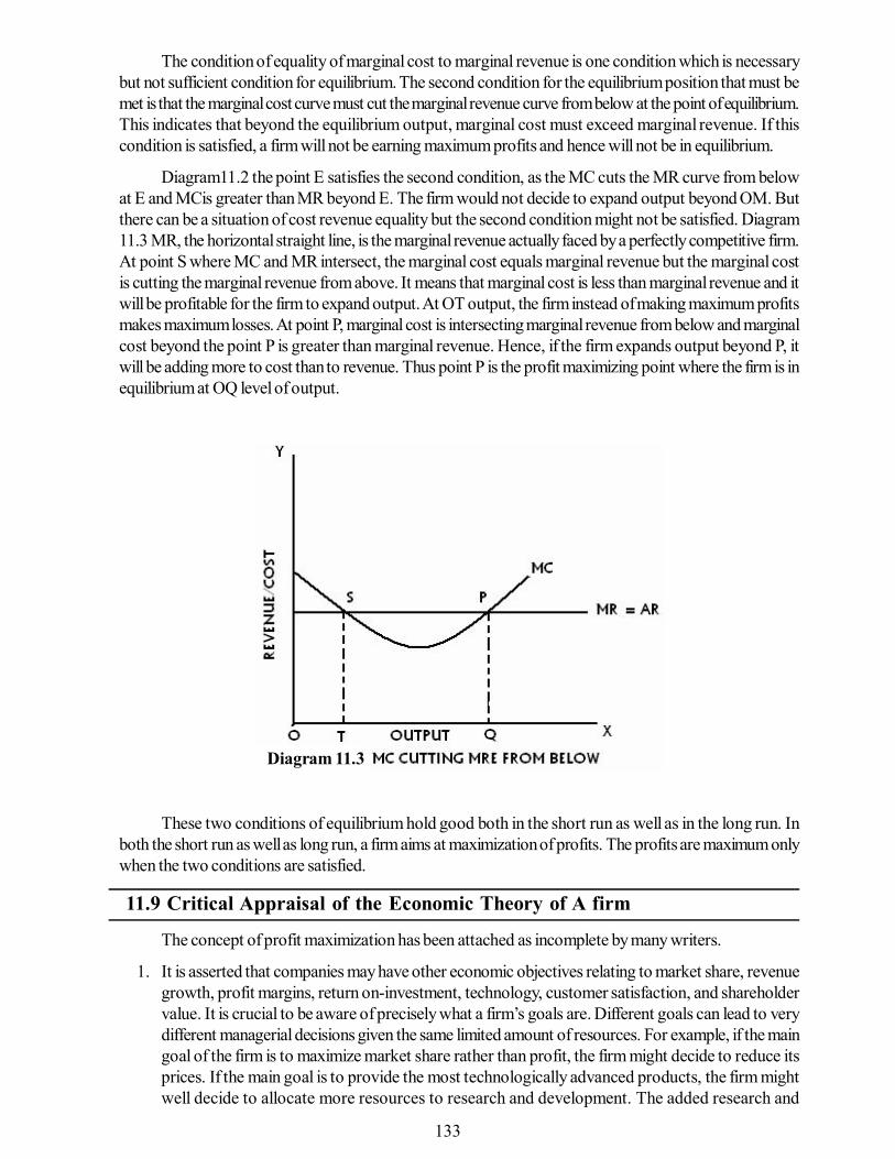
133

The condition of equality of marginal cost to marginal revenue is one condition which is necessarybut not sufficient condition for equilibrium. The second condition for the equilibrium position that must bemet is that the marginal cost curve must cut the marginal revenue curve from below at the point of equilibrium.This indicates that beyond the equilibrium output, marginal cost must exceed marginal revenue. If thiscondition is satisfied, a firm will not be earning maximum profits and hence will not be in equilibrium.

Diagram11.2 the point E satisfies the second condition, as the MC cuts the MR curve from belowat E and MCis greater than MR beyond E. The firm would not decide to expand output beyond OM. Butthere can be a situation of cost revenue equality but the second condition might not be satisfied. Diagram11.3 MR, the horizontal straight line, is the marginal revenue actually faced by a perfectly competitive firm.At point S where MC and MR intersect, the marginal cost equals marginal revenue but the marginal costis cutting the marginal revenue from above. It means that marginal cost is less than marginal revenue and itwill be profitable for the firm to expand output. At OT output, the firm instead of making maximum profitsmakes maximum losses. At point P, marginal cost is intersecting marginal revenue from below and marginalcost beyond the point P is greater than marginal revenue. Hence, if the firm expands output beyond P, itwill be adding more to cost than to revenue. Thus point P is the profit maximizing point where the firm is inequilibrium at OQ level of output.

These two conditions of equilibrium hold good both in the short run as well as in the long run. Inboth the short run as well as long run, a firm aims at maximization of profits. The profits are maximum onlywhen the two conditions are satisfied.

11.9 Critical Appraisal of the Economic Theory of A firm

The concept of profit maximization has been attached as incomplete by many writers.

1. It is asserted that companies may have other economic objectives relating to market share, revenuegrowth, profit margins, return on-investment, technology, customer satisfaction, and shareholdervalue. It is crucial to be aware of precisely what a firm’s goals are. Different goals can lead to verydifferent managerial decisions given the same limited amount of resources. For example, if the maingoal of the firm is to maximize market share rather than profit, the firm might decide to reduce itsprices. If the main goal is to provide the most technologically advanced products, the firm mightwell decide to allocate more resources to research and development. The added research and

Diagram 11.3

134

development expenses would most likely reduce the amount of profit the firms earns in the short runbut may results in increased profits over time as the company increases its technological lead overits competitors. If the main goal of the firm is to carry a complete line of products and services, itmay choose to sell certain produced even though they might not be earning a profit.

2. In the assumption of profit maximization, the concept of profit has never been clearly stated. Is itrate of profit, total or net profits that a firm tends to maximize? The three concepts have entirelydifferent implications for price theory. If the entrepreneur’s share in the total product is taken to beprofit, it is not clear, for the concept of profit itself is not fully settled. Sometimes profit maximizationmeans maximization of money profits. However, profit maximization is not an end in itself. For mostpersons profit is a means to an end and not an end in itself. The majority of entrepreneurs wish thattheir flow of revenue should carry at least the potentiality of a reasonable margin over cost. In somecase of firms, the objective is loss minimization and not profit maximization.

3. With the emergence of corporate form of enterprise, profit maximization as a goal has reduced itsimportance. Other goals have sat on driving seat. This is attributed partly due to the nature of thisform of organization itself. In a corporation there are variety of groups and as many interests- theshareholders, the debenture-holders, the management, and the labor force. The end product is acompromise between them, each interest getting the importance according to its force. In a firmwhere equity holders are in a control of the firm, they may prefer small certain profits to largeuncertain profits. In most joint stock company firm, there is a multiplicity of often conflicting interests

4. A monopolist has no compulsions to maximize his profit. Since a monopolist usually earns super-normal profits, he has no incentive to maximize the profits. In imperfectly competitive market wherebarriers to entry are effective, the firm ordinarily does not have to strive hard for economic profits.

11.10 Summary

A firm is an organization which converts hired inputs into saleable outputs. The inputs are divisibleinto two broad categories- labor and capital. The function of the firm is to hire inputs and convert them intogoods and services for sale. A firm usually follows multiple objectives including profit maximization, salesmaximization, maintaining or increasing its market shares, growing for the sake of growing, creating ormaintaining a desirable financial position, achieving good labor relations and so on. As consumers act tomaximize their utility, the firms act to maximize their profits. Profit is defined as total revenue minus totalcost. The theory of the firm assumes that the firm has single goal- to maximize profit and acts rationally topursue its goal. Rationality implies perfect knowledge of all relevant variables at the time of decision-making, A firm is in equilibrium when it has no incentive either to expand or to contract its output and doesnot like to change its level of output when its total profits are the maximum. There are two approaches toattain a firm’s equilibrium- The Total Revenue-Total Cost Approach and the Marginal Revenue and MarginalCost Approach. In spite of its severe criticism, the profit maximization theory still holds good.

11.11 Key Words

• Firm: A firm represents a business enterprise striving to get the highest profit under particularconditions.

• Profit Maximization: The level of output where marginal revenue and marginal cost are equal isthe point of maximum profit.

• Equilibrium of the Firm: A firm attains equilibrium when it has no incentive either to expandor to contract its output.

• Total Revenue:Total revenue is the outcome of multiplication of price by the number of unitssold.

135

• Total Cost: Total cost is sum of fixed cost and variable cost.

• Break-even-Point: Break-even point is the point where the firm has covered its total cost andstarts earning profit.

• Marginal Revenue: The marginal revenue is the addition to total revenue by selling another unitof output.

• Marginal Cost: The marginal cost is the addition to the total cost by producing another unit ofoutput


1. Explain the economic theory of the firm.

2. Discuss the assumptions of the economic theory of the firm.

3. Describe the multiple objectives of a firm.

4. Critically examine the economic theory of firm.

5. Critically examine the profit maximization doctrine.


1. Mehta P.L., Managerial Economics Analysis, Problems and Cases: Sultan Chand, New Delhi.


136

Unit – 12 Behavioural Theory of a FirmUnit Structure

12.0 Objectives12.1 Introduction12.2 The Firm : Objectives and Constraints12.3 Value Maximisation12.4 Size Maximisation12.5 Long-run Survival12.6 Theories of A Firm Behavioural12.7 Problems in Profit Measurement12.8 Profit Maximisation as Business Objective12.9 Theory and Practice of Profit Maximisation Objective12.10 Summary12.11 Key words12.12 Self Assessment Test12.13 Suggested Books / References

12.0 Objectives

After studying this unit, you should be able to understand :

• The concept of a firm.• Objectives and constraints of a firm.• Problems in profit measurement.• Theory and practice of profit maximisation objective.

12.1 Introduction

The classification of a firm is done on the basis of ownership, management and control. Firms canbe classified into categories like private sector firms, public sector firms, joint sector firms and non-business firms. On the basis of the ownership they are known as proprietorship, partnership and corporations.Universities, public libraries, hospitals, performing arts groups, museums, churches, voluntary organisations,cooperatives, credit unions, labour unions, professional societies, foundations and fraternal organisationsare also understood as group of firms. Such organisations provide services to a group of clients or servicesto members only. Such classification of firms help us in understanding the objectives of firms.

The output of firms comprises goods and services wherein five factors of production namely land,labour, capital, entrepreneur and organisation are employed. Labour, entrepreneur and organisation areknown as human factors of production while natural and man made resources are a part of capital resources.

Thus the production of goods and services is the result of the collective efforts of these five factorsof production. The problem of choice of technique of production also arises depending upon the input mixfrom all alternatives each firm has.

12.2 The Firm : Objectives and Constraints

Traditional theory of firm assumes profit maximimsation, as the sole objective of business firms. ButProf. Baumol has argued that it is not correct to say that all business firm pursue the same objective.

137

Recent researches have revealed the fact that the objectives of business firms are more than one. Thereare a number of theories propounded about the objectives of a firm as given under :

(i) Profit maximisation(ii) Firm’s value maximisation(iii) Sales maximisation(iv) Size maximisation(v) Long run survival(vi) Management utility maximisation(vii) Satisfying(viii) Other (non-profit) objectives

Profit Maximisation

Profit is a comprehensive term and it has different meaning to businessmen, accountants, tax collectors,workers and economists. ‘Economic profit’ and ‘accounting profit’ are generally used for decision makingin business activities.

The formula for calculating accounting profit is as given under :

Accounting Profit = TR — ( W + R + I + M )

where W stands for wages and salaries, A stands for rent, I stands for interest and M stands for costof materials.

While calculating the accounting profit only explicit or book costs are taken into consideration.Economic profit is wider than accounting profit wherein implicit costs are also included. Economic profitmakes provision for insurable risks, depreciation and necessary minimum payment to shareholders toprevent them from withdrawing their capital. It’s also called pure profit. The economic profit is calculatedwith the help of the following formula :

Economic/Pure Profit = Total Revenue — (Explicit Costs + Implicit Costs)

Example : A carpenter makes 150 chairs per month and sells them at Rs.100 per piece. His expenseson rent of the shop, costs of wood and other material are worth Rs.4000. He employs two workerswhose monthly wage bills stands at Rs.3000 and pays electricity bill of about Rs.500 per month. He hasinvested Rs.40000 in the form of machines, tool and inventories in the business of which Rs.25000 is fromhis own fund and remaining Rs.15000 is a loan from a bank at the interest rate of 18% per annum. Furtherassuming imputed costs of his own time, his wife’s time and his own savings of Rs.25000 for the month areRs.3000, Rs.1000 and Rs.250 respectively. The various calculations would then be:Total Receipts= Rs.100 x 150 = Rs.15000Total explicit costs = Rs.4000 + 3000 + 500 + 15000 (0.18)

12= Rs.7725

Total implicit costs = Rs.3000 + 1000 + 250= Rs.4250

138

Business (Accounting) Profit = Rs.15000 – 7725= Rs.7275

Economic Profit = Rs.15000 – 7725 – 4250= Rs.3025

Thus, business and economic concepts of profit are different. In this chapter we will use profits onlyin its economic sense.

Economic profits are a powerful instrument in the free enterprise system, particularly for aproprietorship firm. At present we have both private and public sector firms. The public sector firms areknown to pursue social objectives such as factor productivity and the supply of essential goods at reasonableprices.

Firm’s Constraints

Firms while making decisions are faced with certain restrictions or constraints. Such constraints areinternal and external. The internal constraints are concerned with the organisation of the firm. What is to beproduced? Where is to be produced? For whom is to be produced? How much is to be produced?

External constraints are related to resource constraints, output quantity or quality constrains, legalconstraints and environmental constraints.

12.3 Value Maximisation

Most of firms are expected to operate for a long period. They are interested in maximisation of longterm profits instead of maximum short term profit. Value of the firm can be calculated with the help of thefollowing formula :

Value of the firm = P1 + P2 ..... Pn

(1 + i) (1 + i)2 (1 + i)n

P1 stands for expected profit in period 1, P2 is expected profit in period 2 and so on. i is the cost ofequity capital. The concept of discounting and present value are taken into consideration. Wealthmaximisation is recognised at the primary objective of a business firm. Non-business firms also pursuenon-value maximisation objectives.

12.4 Size Maximisation

Some experts have suggested growth or size maximisation as one of the alternative goals for abusiness firm. Growth means an increase in sales, assets and the number of employees. Edith Penrose hasrightly pointed out that managers have a vital interest in growth because individuals gain prestige, personalsatisfaction in the successful growth of the firm with which they are connected, more responsible andbetter paid positions, and wider scope for their ambitions and abilities.

12.5 Long Run Survival

This alternative goal for the firm has been suggested by K.W. Rottschild which assures long runsurvival for the firm. According to this concept the firm seeks to maximise the probability of its survival into

139

the future. This objective is in the interest of the share-holders and the management. The owners of thebusiness provide security and business to their next generations. The present and future compensationdepends on the firm’s continued existence. The measurement of long run survival is difficult in practice.

12.6 Behavioural Theories of A Firm

These theories were given by a noble prize winner Herbert Simon in 1956. R.M. Cyert and J.E.Mareh Firms can not maximise profits, sales etc. due to imperfections in data and incompatibility ofinterest of various constituent of an organisation. The firms should satisfy all the constituents of the firmcomprising of the stock holders, management, employees, customers, suppliers and government.

This objective is a multiple goal and it is very difficult to practice and achieve. Human beings wantsatisfaction not only in an absolute sense but in a relative sense as well. The different constituents of abusiness firms have diversified interest.

12.6.1 H.A. Simon’s Satisfying Behaviour Model

According the satisfying behaviour model given by Simon, managers in their business decision-making are constrained by the factors like incomplete information, imperfect data and uncertainty aboutthe future. The management determines a ‘satisfactory aspiration level’ on the basis of its past experienceand judgement about the future uncertainty. They, therefore, seek a second best solution which is calledthe satisfying behaviour.

The satisfactory behaviour holds that a manager will aim for:

(i) a satisfactory level of profit maximization.(ii) A satisfactory level of cost rather than cost minimization.

If the satisfactory aspiration level is a achieved easily, the expiration level is revised upwards. And ifthe satisfactory aspiration level is not achieved or upward as well as downward revisions, the managementindulges in ‘search behaviour’ to find the reasons for the deviations from the aspiration level

Simon suggests that if the satisfactory state is not achieved even by lowering the aspiration level andthe search behaviour. The behaviour pattern of managers becomes that of apathy or aggression.

The model is positive in the following manner:

(i) the model explains certain real-world situation. For example, the firms generally use make-up pricingto generate reasonable profits rather resort to marginal cost pricing to maximize profits.

(ii) Model is consistent with the theory of motivation where human action is a function of derives and itterminates when derives are satisfied.

However, there are serious flaws with the theory of satisfying behaviour as given below:

(i) the model lakcs correctness and complete information. It does not identify the types of informationthat are sought by a firm and nature of ‘incompleteness’ the information suffer from.

(ii) The model fails to appreciate the difference between information about conditions and informationabout changes in conditions. It is the information regarding changes in conditions that is vitally moreimportant.

(iii) ‘Satisfactory level’ is a subjective concept. It depends of many factors like industry one is talking

140

about, the economic situation, the nature of top management, the perception of the decision-makingmanager etc.. in each a case the comparison of managerial behavioural becomes a problem.

12.6.2 Cyert and March’s behavioural theory of firm

The behavioural model of the firm, propounded by Simon, has subsequently been elaborated byCyert and March in the behavioural theory of firm (1963)

The behavioural theory of Cyert and March focuses on the way decisions are made in the modem,large multi-product firm underuncertainty in an imperfect market.

Cyert and March base their theory on the internal structure of such firms and try to analyse thetypical organizational problems which the intemal structure of such firms creates and the effects of theseproblems on the decision-making process. They explain the difference in reactions of different firm,tothe same set of extemal forces in terms of the differences in intemal organisatonal factors.

R.M. Cyert and J.E. March consider the firm as a multi-goal, multi decision organizational coalition.onsists of the various groups associated with the firm like managers, workers, shareholders, customers,suppliers, bankers, lawyers, accountants and so on each group has its own set goals. Cyert and marchpoint out that the most significant groups in the decision making are: shareholders and workers.

Goals of the firm : Satisfying behaviour

The behaviour theory of the firm starts with a recognition that individual members of thecoalition-firm have different goals to that of the organization coalition. According to Cyert and Marchgoals of the firms are determined by the demands of individuals in coalition.

The top management in the mode corporate firm enjoys the ultimate authority to act the goals of thefirm. According to Cyert and March there are five major goals of term as under:

(i) Production goal- is set by the production unit of the firm.

(ii) Inventory goals- is set by the inventory unit of the firm.

(iii) Salare of the market goals- is set by the sales unit of the firm.

(iv) Share of the market goals- is set by the sales unit of the firm.

(v) Profit goals- is set by the top management keeping in view the expectations of the shareholdersbankers and other financial institution. It is the ultimate goal of each firm.

Like goals of individuals, the goals of the firm also undergo a change overtime. As the number ofgoals of the firm increases, the decision-making process becomes increasingly complex and consequentlythe efficiency of decision-making decreases. The goals of the firm are ultimately decided by the efficiencyof decision-making decreases. The goals of the firm are ultimately decided by the top management throughcontinuous bargaining between the groups of coalition. The top management tries to accommodate asmany of the conflicting demands as possible.

Cyert and March model is also a satisfying organization and not a maxiimsing organization likeSomon’s model. It compares its performance with the set goals. In case the goals have not been met asearch activity begins to find out the reasons for the non-fulfilment of the target . If it is found thatnon-fulfilment was due to factors outside the control of the firm, a downward revision of the goals likelyfor the next period is made.

141

In the organization-coalition if there is often a conflict of goals it needs to be overcome. Cyert andMarch suggests two ways in which the conflict can be avoided:

Conflict may be phase out overtime in the sense that they are dealt with one by one, as they arise.

Conflicts may be segregated to diffuse their impact on the whole organization. Each conflict may belocalized into its respective department and decisions taken accordingly.

For smooth working in the organization, there is some decentralization of decision making. However,at the lower administrative levels managerial staff follows standard procedures stated in blue prints. Rulesof the thumb aim at ensuring working that is consistent with the goals set by the top management.

In the process of decision making. The following controversial points create doubts about themerits of the behavioural theory:

(i) Investment decisions are usually based on long –term considerations which this theory ignores in itseagerness to avoid role of uncertainty in decision making.

(ii) An adjustment of aspiration levels when costs and demand adjustment fail, implies that anyperformance of the firm can be considered satisfactory. This is a questionable proposition becausedownward revision of the goals to lower satisfying levels may not be acceptable to various groupsdespite the firm’s claim that it did its best under the circumstances.

(iii) By constant revision in the satisfying level, the criterion on which the top management sets the goalsof the firm loses its relevance.

(iv) Estimates of costs and rules of their upward or downward adjustment are simplistic and mechanical.

(v) Forecast of demand in the current period are simply extrapolation of the demands in the previousperiods in estimating current demand, no allowance is made for future uncertainty.

Criticism of Cyert and March behvaioural theory:

Cyert and March are the leading exponents of the behavioural theory. Cyert and March based theirtheory on four actual case studies and two experimental studies conducted with hyponthetical firms. It isthus, obvious that their attempt to develop a generalized behavioural theory of firm is flawed by lack ofadequate empirical evidence.

The behaviour theory suffers from the following weaknesses and criticisms:

(i) The behavioural theory follows a simulation approach to analyse the working of a multi-productfirm. Simulation is a predictive technique and is not appropriate for explaining the behaviour ofthe firm.

(ii) The behvaioural theory is concerned with the short run which is unrealistic for dealing with uncertainty.The firm must take a long run view of the environment.

(iii) The behavioural theory does not deal with equilibrium of the industry.

(iv) The theory does not explain the interdependence of the firms and thus simply ingress their interactions.

(v) The behavioural theory does not examine the implications of potential and real threats to establishedfirms.

(vi) The behavioural theory suggests multiplicity of goals for a modern corporate which is basicallyincorrect and miseading.

142

(vii) The theory attempts to resolve to resolve the problem of olgopolistic interdependence by assumingtacit collusion of firms which is not valid in all cases. An oligopolistic theory may also be non-collusive.

(viii)The adjustment of aspiration levels downward whenever the goals are unattable implies that thereis no objective criterion to judge the satisfactory performance.

(ix) Search is usually problem oriented and on this issue, the behavioural theory takes a realistic position.

Thus, in brief we may comment that Cyert and March model suggests that the firm attempts toachieve multiple goals and managers are content to achieve satisfactory levels of these multiple tatgets.The model considers firm as an ogranisational coalition consisting of various groups, each group having itsaspiration level, the goals of the firms are arrived at by the process of continuous bargaining betweengroups of the coalition, wherein as many conflicting demands of the various groups as possible areaccommodated.

12.7 Problems in Profit Measurement

As we know accounting profit equals revenue minus all explicit costs and economic profit equalsrevenue minus explicit and implicit costs. Once profit is defined, it should not be difficult to measure theprofit of a firm for a given period. The measurement of profit becomes difficult due to two reasons as givenbelow:

(i) which concepts of profit be used for its measurement?

(ii) what costs should be and what should not be included in the implicit and explicit costs?

The profit concept to be used for the measurement is the purpose for which such measurement isneeded. Accounting concept of profit is used from the point of view of the shareholders, financiers, creditors,managers and tax liability. Necessary revenue and cost data are essential to calculate the accountingprofit. If we want to measure ‘true profit’ the concept of economic profit should be used. This can be usedwhen the ownership of that investment or business is fully terminated. But in practice the life of a corporationis eternal. It can be measured only on the basis of maximum amount that can be distributed in dividends.Depreciation, capital gains and losses and current v/s historical costs are the items of cost and revenuewhich are taken into consideration for the measurement of accounting profit.

12.8 Profit Maximisation as Business Objective

Various price and production theories of economies have been propounded by economists thatprofit maximisation is the most important assumption. Traditional economics assumes profit maximisationas the only objective of business firms. It has been a long history in economics. This objective is consideredas the most reasonable and analytically the most productive business objective. It helps a business firm inpredicting its behaviour as well as the behaviour of price and output under different market structure.There is no alternative to explain and predict such behaviour.

12.9 Theory and Practice of Profit Maximisation

W have discussed that traditional theory assumes profit maximisation as the sole objective of abusiness firm. But now business practices have undergone a drastic change and firms are pursuing objectivesother than profit maximisation. In the large corporations the ownership and management are separate andthe goals for the firms they manage are set other than profit maximisation. For examples sales maximisation,

143

maximisation of utility function, maximisation of firm’s growth rate, making a target profit, retaining marketshare, building up the net worth of the firm etc. are other goals of business firms.

The traditional economics is based on the assumption of perfect competition which is unrealistic andimaginary. The marginal principle of equalising marginal cost and marginal revenue (MC = MR) is alsoabsent in the decision making process of the firms. Thus there is little link between pricing theory andpricing practices.

12.10 Summary

Classification of a firm can be made on the basis of their management, ownership and control. Theyare proprietorship, partnership and corporations. The output of firms comprises goods and services whereinfive factors of production namely land, labour, capital, entrepreneur and organisation are employed. Thereare several objectives a firm namely profit maximisation, firm’s value maximisation, sales maximisation,size maximisation, long run survival, management utility maximisation and non-profit motives as well. Abusiness firm faces constraints both internal and external. These areproduction decision, raw materials,quantity and quality constraints, legal and environmental constraints.

12.11 Key Words

• Classification : Categorization of business firms.

• Constraints : Hurdles or obstacles while carrying on the activities by business firms.

• Profit Maximisation :Difference between the total revenue and total cost of a business firm.

• Explicit Costs :Remuneration paid to hired inputs.

• Implicit Costs : Remuneration calculated at market price for owned factors of production.


1. Give the classification of a firm.

2. Discuss the objectives of a business firm.

3. Differentiate between accounting profit and economic profit.

4. What is profit maximisation?

5. Differentiate between value maximisation and size maximisation.

6. Discuss the problems in profit measurement.

7. Write a note on theory and practice of profit maximisation.

8. Describe H.A. Simons satisfying Behaviour Model

9. Critically examine Cyert and March’s behaviour theory of a firm.



2. Mehta P.L., Managerial Economics Analysis, Problems and Cases, Sultan Chand, New Delhi

144

Unit – 13 Managerial Theory of a FirmUnit Structure

13.0 Objectives13.1 Introduction13.2 Managerial Aspect of a Firm13.3 Managerial Utility Function13.4 Marris’s Theory of Managerial Enterprise13.5 Willamson’s Theory of Managerial Discretion13.6 Principal Agent Problem13.7 Reasonable Profits13.8 Profit as Control Measure13.9 Baumol’s model of Sales Revenue Maximisation13.10 Summary13.11 Key words13.12 Self Assessment Test13.13 Suggested Books / References

13.0 Objectives


• The concept of managerial aspect of a firm.• Managerial utility function.• Principal agent problem.• Reasonable profits.• Profit as control measure.

13.1 Introduction

The members of the board of directors are agents of the share holders. They monitor the decisionsof executive managers. Managers are also agents of owners and directors. It creates agency problemsbetween different agents in a business organisation. When business decisions are complicated, theeffectiveness of a board of directors is undermined.

Value maximisation decisions are based on the corporate policy on debt financing. If a business firmis financed with debt rather than equity, it increases the interests of shareholders in various ways.

13.2 Managerial Aspect of a Firm

Managerial aspect of a firm deals with the production decisions, exchange decisions and consumptiondecisions. Most decisions involve a time dimension. Production decision requires an understanding of themarket for various commodities in future which is uncertain. A business firm from the managerial point ofview has to take decisions regarding the production, exchange and consumption so that the ultimate goalof maximisation of profit and the social responsibility of business firm are also attained. Planning, organisation,direction, coordination, motivation, control and decision making are some of the managerial aspect of afirm to be performed in a rational way. These are the basic roots of the business firm for its survival in thelong run, satisfying the needs of all the parties directly indirectly by being connected with it.

145

13.3 Managerial Utility Function

This model was propounded by Oliver Williamson. It is a combination of the objectives of profitmaximisation and growth maximisation. This model emphasizes upon the fact that in modern businesses,ownership is different from management and modern managers have discretionary powers to set the goalsof firms. According to this model managers would apply their discretionary power in such a way, as tomaximise their own utility function, with the constraint of maintaining minimum profit to satisfy shareholders.The utility function of managers depends upon their salary, job security, power, status, professional satisfactionand the power to influence firm’s objectives. Williamson has given the model in the form of a formula asgiven below:

UM = f (S, M, ID)

where UM is manager’s utility function S is salary, M is managerial emoluments and ID is power ofdiscretionary investment.

This theory has certain weaknesses. The model fails to deal with the problem of oligopolisticinterdependence. The theory holds good only where rivalry between firms are not strong. This modeldoes not offer a more satisfactory hypothesis than profit maximisation.

13.4 Marris’s Theory of Managerial Enterprise

Growth of the firm is obviously the cornerstone of corporate strategy. The goal of the firm is themaximisation of the balanced rate of growth of the firm. Marris interprets the goal as the maximisation ofthe rate of growth of demand for the firm’s products and the growth of its capital supply.

Marris’s hypothesis is that, executive actions are limited by the need for management to protect itself from dismissal or take-over raids in the event of failure. Marris tried to omprove upon Ballmol’smodel. He offered a variation of Baumol’s model that stressed the maximisation of growth subject to thesecurity of management’s position. Marris approach is also based on the fact that ownership and controlof the firm is in the hands of two different set of people.

Like Williamson, Marris suggests that managers have a utility function in which salary, status power,prestige and security are important variables. Owners of the firm (shareholders) are however, more con-cerned about profits, market share, output etc. In other words, goals of the managers and shareholdersdiffer from each other. The utility function of managers (Um) and that of the owners (Uo) may, therefore,be defined as :

Um = f (salaries, power, status, job security)

UO = f (Profits, market share, output, capital, public esteem).

Robin Marris believes that most of the variables entering into the utility function of managers ownersare strongly correlated with a single variables : the size of the firm. He, therefore states that the managerswould be mainly concerned about the rate of growth of size.

Marris takes the view that the owners being interested in the growth of the firm want maximisationof growth of the supply of capital which is assumed to maximise their utility. Th utility function of ownersmay be depicted as follows :

UO (f (gc)

146

Where, UO = utility of owners, gc = rate o growth of capital.

Managers want to maximise rate of growth of the firm rather than absolute size of the firm. Theybelieve that growth of demand for the products of the firm is an approrpiate indicator of the growth of thefirm. Further, salaries, status and power of managers are strongly correlated with the growth of demand.The managerial utility function can be illustrated as under :

Um = f (gD, s)

where, Um = utility of managers.

gD = rate of growth of demand for the products of firm

s = a measure of job security.

Marris has suggested that the decision making capacity of the managerial team sets a constaint torate of growth of demand for the products of firm. Further more, he argues that job security can bemeasured by a weighted average of the liquidity ratio, the leverage / debt ratio and he profit retention ratiowhich together reflect the financial policy of the firm.

Marris assumes that there is a saturation level of job security. Below the saturation level marginalutility from an increase in job security is infinity while above the saturation level it is zero. With thisassumption, Marris considers job security an exogenously determined constraint. The marginal utilityfunction thus becomes.

Um = f (gD) s , where s is the security constraint.

In Marris model, there are two constraints :

(a) The managerial team constraint

(b) The job security constraint

(a) The managerial team constraint : Marris is of the view that the capacity of the top managementis given at any one time period. Since management is a team work, hiring new managers does notexpand the managerial capacity immedaely. New managers take time to get integrated in the teamwhich is extremely essential for the efficient working of the firm.

Moreover, the research and development (R & D) department also sets a limit to thegrowth of managerial capabilities of the firm. The managerial team constraint sets limits to both therate growth of demand for the products of the firm (gD) and the rate of growth of capital supply(gc).

(b) The Job Security Constraint : Managers want job security. Their desire for security is reflectedin the preference for service contracts, generous retirement benefits and their dislike for policieswhich may result in their dismissal. Job security is assumed to be attained by pursuing a prudentfinancial policy which requires that the three crucial finanical ratios must be maintained at optimumlevels.

Ratios :

To judge the prudence of a financial policy, Marris proposes the concept of financial constraint (i)which is mainly determined by the risk attitude of the top management. A risk-loving management wouldprefer a high value of a, while a risk averting management would prefer a low value of Marris defines ‘a’

147

as the weighted average of the following three ratios :

Liquidity Ratio (a1) = LiquidityAssets

TotalAssets

Leverage Ratio (a2) = ;ValueofDebts andTotal Assets

Profit - Retention Ratio (a3) = Re Prtained ofits

Total Assets

The low liquidity ratio, that is, the ratio of liquid assets to total assets increases the risk of solvency.Likewise, a high leverage / debt ratio, that is, the ratio of debt to value of total assets, poses the firm to ahigh degree risk of bankruptcy. A high retention ratio which refers to the ratio of retained profits to totalprofits, contributes most to the growth of the firm’s capital.

According to Marris’ managers subjectively assign weights to financial ratios and comine them intoa single parameter a , which is called the financial security constraint, a is negative lynelated liquidity ratioand positively to leverage / debt ratio and retention ratio. Morevover, there is a negative relation betweenjob security (S) and the financial security constraint a . Thus a Low value of a implies that the managersare risk averters while a high value of a means that the managers are risk takers. In Marris model, thefinancial security constraint a sets a limit to growth of the supply of capital gc. ( a is financial securitymanagement).

Equilibrium of the Firm :

The managers of corporate firm aim at maximisation of their own utility which is a function of thegrowth of demand for the product of the firm, given the job security constraint

Um - f (gD)

The shareholdrs of corporates aim at maximisation of their own utility which according to Morris, isa function of the growth of the supply of capital.

The firm is considered to be in equilbrium when it attains the maximum balanced rate of growth.Thus, the condition for equilibrium of the firm may be writen as follows :

gD = gC = g* maximum

In order to follow the above condition for the equilibrium of the firm, it is necessary to grasp thefactors that determine gD and gC. Marris argues that the two variables, the diversification rated, and theaverage profit margin, m, adequately represent the factors that determine gD and gC.

Marris suggests that the corporate first decides subjectively its financial policy. In other words thefirm first determines the value of the financial constraint a . Subsequently, the rate of diversification ‘d’ andprofit margin ‘m’ will be chosen.

To achieve balanced growth rate would be to identify the factors that go in to determine gD and gC.According to Marris, these determines can be expressed in terms of two variables :

a) Diversification rate (d) ; and

(b) Average profit margin (m)

148

Both thes variables can be, however determined only after the management has decided about itsfinancial policy, a. The diversification rate can be chosen either by changes in style of the production cost,the average profit margin would be affected by the levels of advertising and D, Higher the expenditure onadvertisement (A) as well as R and D, lower would be the average profit margin (m). Thus, the Marris’firm three policy variables : a, b and m.

Marris also points out that there can be a conflict between managers’ objective of maximisinggrowth and shareholders’ objective of maximising profits. Therefore, if the growth maximising solutiondoes not generate sufficient profits, growth rate will have to be reduced to increase given to meetshareholders expectations.

In brief, in Marris model, the management, whose actions are limited by the motivation to protect ititself dismissed or take-over bids, takes to the following course :

(a) The management must walk on a knife-edge between a debt/asset ratio high enough to stimulategrowth but not low enough to suggest financial imprudence.

(b) The management must also maintain a low liquidity ratio, i.e., liquid asset/total assets. But this ratiomust not be so low that it endangers paying all obligations on time.

(c) The management must try to keep a high retention ratio, viz. retained earnings/total profits. But thisratio should not be so high that shareholder are not paid satisfactory (gd) and growth rate of capitalsupply (g) :

Max. g = gd = gc

g = balanced growth rate

gd = growth of demand for products

gc = growth of supply of capital

By this process the managers achieve maximisation of their own utility as well as that of the share-holders. In case the management wants to exapand too rapidly, it runs the risk of job security. On the otherhands, if it wants to expand too slowly, it would be considered as an inefficient management, again impair-ing job-security.

13.4.1 Criticism of Marris Theory

R. Marris has made a significant contribution in the form of incorporation of financial policies intothe decision making process of the corporate firm. His theory suggests that although the managers and theowners have different goals, it is possible to find a solution which maximises utility of both. Still there arecertain weaknesses of the theory as under :

(i) The assumption of given production costs and a price structure is the weakness of Marris theory.

(ii) Marris theory does not exaplin the determination by either costs or prices.

(iii) A Koutsoyiannis criticises that oligopolistic interdependence is not satisfactorily dealt with, withinMarris ‘ Model.

149

(iv) Marris brushes aside the mechanism by which prices are determined.

(v) Marris’s assumption that the growth of the firm is achived mainly via the introduction of newproducts which will be imitated by competitors, does not hold the ground.

Thus the maximisation of the goal of balanced growth (maximise g = gd = gs) is that by jointlymaximising the rate of growth of demand and capital, managers achieve maximisation of their own utility aswell as utility of the shareholders.

In both the Baumol and Marris models, the long-run growth of the firm and its ability to stafisty itsconstrains depend upon the continued availability of large stream of profits. It seems clear, that whateverdifferences may exist in the short-run interests of growth-maximising, sales maximising, or profit maximisingfirms, their long-run interests and decisions are virtually the same. Products that attempts to maximisesales or assets in the long-run will maximise profits.

13.5 Williamson’s Theory of Managerial Discretion

O. Williamson evolved a more useful model of managerail utility better known as the ‘Model ofmanagerial Discretion’. As per the basic concepts of the model, managers are free to pursue their ownself-interest once they have achieved a level of profit that will pay satisfactorily dividends to theshareholders and still ensure growth.

The managers self interests depend upon many other things besides salary. Further, so far as thegoodwill of the firm serves their own ends and amibitions, the managers would be concerned about it, elsethey would try to byepass it.

Williamson is of the view that the managers of a present day business firm, which is organised acorporate unit do not maximise the profits which results in the maximisation of the utility of the owners.Instead, they maximise their own utility using their discretion. However, for their job security managersattempt to ensure a certain mnimum amount of proit to shareholders, in the form of dividend. The profitworks as a constraint to the manager’s decision.

Managers utility depends on variables such as ; job security, power, prestige, status, job satisfactionand professional excellence. Among those variables, only salary can be measured, other variables arenon-measurable. Therefore, Williamson uses measurable variables like staff expenditure, managerialemouluments and discretionary investment in the utility function of managers on the assumption that theseare the sources of the job security and reflect power, prestige, status and professional achievements ofmanagers.

Assumptions of the model

Like Baumol, Williamson also adopts in following assumption in his model :

(i) Market is non-perfectly competitive.

(ii) Ownership of the firm and management of the firm are divorced from each other.

(iii) A minimum profit constraint is imposed on the managers by the capital market (or shareholders)which cannot be ignored by the management.Williamson puts the utility function of the managers as follows :

U = f (S, M ID)

150

whereS = staff expenditure including managerial salariesM = managerial emolumentsID = discretionary investment

Basic Concepts

The basic concepts and relations of the management utility function ( U = f (S, M , ID) is producedas under :

The Demand for the Firm :

The firm’s demand curve is assumed to be downward sloping and is defined by the function as :

X = f1 (P, S, e)

or P = f2 (x, S, e)

where :

x = output, P = Price, S = Staff expenditure

(2) Oe = a demand shift parameter reflecting autonomous changes in demand.

The demand is negatively related to price and is assumed to be positively related to staff expendi-ture and to the shift factor.

The Production Cost :

The production is assumed that the total production cost is an increasing function of output.

( )3C f X=

where C OX

¶ >¶

Various Concept of Profit :

The relevant concepts of profit are :

(i) Actual profit p (ii) Reported profit Rp (iii) Minimum profit Op (iv) Discretionary profit Dp (i) The actual profit p , is sales revenue (R) minus production cost (C) and minus staff expenditure (S)

(ii) The reported profit Rp , is the profit that the firm reports to the tax authorities. It is the actualprofit minus tax deductible managerial emoluments (M)

–R Mp p=

or = R - C - S - M (by putting)

151

Thus, Rp = R - C - S - M

(iii) The minimum profit Op , is required to satisfy the shareholders. If this profit is not earned, theshareholders will either sell their shares or change top management, adversely affecting to the jobsecurity of managers.

O R Tp p£ -

where T = tax

(iv) The discretionary profit Dp , is the amount of profit left after subtracting the minimum profit ( )Op

and Tax (T) from the actual profit ( )p .

– –D O Tp pp=

The discretionary investment (ID)

The discretionary investment is the amount that is left from the reported profit Rp after subtractingthe minimum profit ( )Op and the tax (T)

0DI R Tp p\ = - -

13.5.1 Williamson’s Model of Managerial Discretion

In Williamson’s simplified model, it is assumed that managerial emoluments are zero (M = 0) andthus, the actual profit is the same as reported profit.

The simplified model may be as follows :

Maximise U = f (S, ID)

subject to O Tp p³ +

Since, it has been assumed that there are no managerial emoluments (M = O), all the discretionaryprofit ( )Dp gets absorbed in discretionary investment ( )DI . Thus, the managerial utility function may bewritten as :

{ }– –U f O Tp p=

For simplicity it is assumed that there is no lump sum tax so that T tp=

Thus, the managerial utility function assumes the form

( ){ },U f S I t Op p= - -

where,

(I - t) O Dp p p- = is the discretionary profit.

Equilibrium of the firm : Graphical Presentation.

The equilibrium of the firm in Williamson’s model can be shown graphically as under, whichrequires:

152

(i) Construction of indefference curve map of the managers in which such curves show thecombinations of staff expenditures (S) and discretionary profit Dp providing a certain level ofutility; and

(ii) The discretionary profit - staff curve.In the diagram 13.1, the indifference curve of managers is shown as below :

Diagram 13.1

In the diagram 14.1 staff expenditure (S) is shown on X-axis and discretionary profit (PD) on Y-axis.Each indifference curve (U) is convex to the origin which implies diminishing marginal rate of substitution ofS for Dp .

(i) It is assumed that indifference curve do not intersect each other.(ii) It is also suggested that managers choose only the positive value of S and Dp in theirutility function.Similarly, the relationship between the discretionary profit ( )Dp and staff expenditure (S) may be

depicted in the diagram 13.2

Diagram 13.2

Disc

retio

nary

Pro

fit

Staff expenditureIndifference curve of Managers

Y

X

UU

UU

4 3

21

AS

B

C X

Y

Disc

retio

nary

Pro

fit

Staff expenditureRelationship between and SrD

153

The relationship between the staff expenditure (S) and sicretionary profit ( )Dp (as shown in thedigram 14.2) may be determined by the profit function.

( )f Xp =

=f (P, S, e)

The minimum profit Op and tax t are exogenously by the shareholders demand for dividneds andthe tax laws.

It is assumed that the output is chosen optimarlly according to the marginal rule MC = MR and themarket environemtn is given (e). The relationship between Dp and S is shown in the above diagram. Itmay also be observed in the diagram that in the initial stages of production and upto the point where profitsreach their maximum level i.e., BS, both discretionary profits and staff expenditure increase. Once pro-duction expands beyond this point, the discretionary profit falls while staff expenditure continues to in-crease.

Now we can rightly show the equilibrium of the firm in the diagram. 13.3

Diagram 13.3

The equilibrium of the firm in Williamson’s model is determined by the point of tangency of theprofit-staff curve Ps as shown in the diagram as above and the highest possible managerial indifferencecurve U4. This point is E at U4 indifference curve.

Under equilibrium, the firm’s total discretionary profit is ES2 which is smaller than the total profitBS1 which the firm would earn in profit maximising mode. In Williamson’s model, the staff expenditureOS2 will be greater than that of a profit maximiser OS1.

Koutsoyiannis commenting on Williamson’s model states, “Williamson’s model is applicable in mar-kets where rivalry is not strong, or for firms which have some advantage over their rivals. However, in thelong-run such advantages which sheter a firm from competition are usually weakened, and competition isenhanced. When rivalry is strong a profit maximising model may be more apropriate unless some from ofcollusive agreement is achieved and firms adhere to it.

Disc

retio

nary

Pro

fit

Staff expenditureEquilibrium of the Firm

Y

X

UU

UU

4 3

21

Y S1 S2 PS

EBR

154

Williamson’s model no doubt brings in foucs corporate managers’ power to exercise theirdiscretion for the maximisation of their utility, but it fails to deal with the core problem of oligopolisticinterdependence and of strong oligopolistic rivalry.

Thus, Williamson’s model suggests that a firm led by utility-maximising managers spends more onstaff expenditure and exhibits more organisational slack than a profit - maximising firm. Evidence providedby Willliamson in support of this theory is not fully convincing. The theory of Williamson’s ManagementDiscretion’ has at least one serious flaw, i .e. the measure of executive compensation does not providesufficient importance to non-salary components of the compensation, consequently, it may significantlyunder estimate the profit-maximising behaviour of managers in the real wold. The managers are expectedto follow policies which maximise their utility function.

13.6 Principal Agent Problem

We are aware that there is conflict of interests between the owners and the managers of a firm.According to Williamson’s hypothesis managers are more interested in maximisation of their own benefits,instead of miximising profits of the corporate world. This is an example of a principal agent problem whicharises in the context of firms. The consumers are the principal and service provider is agent In anybusiness organisation owners are the principal while managers are the agents. An agent is hired to executea particular task because he has better knowledge about the task. In a business firm owners hire managerswho work on a well defined task because they have better knowledge of the market and are expected tosteer the business.

13.7 Reasonable Profits

Modern large corporations aim at making a reasonable profit rather than maximizing the profit.According the professor Joel Dean has given the following reasons for reasonable profits :

(i) Preventing entry of competitors.

(ii) To present a favourable public image.

(iii) To put restrictions on trade union demands.

(iv) To maintain customer goodwill.

(v) Other factors namely managerial utility function, harmonious relation between executives and tomaintain internal control over management by restricting firm’s size and profit.

13.8 Profit as Control Measure

An important managerial aspect of profit is its use in measuring and controlling performance of theexecutives of the large business undertakings. Researches in the field have revealed that business executivesdeviate from profit objective and try to maximise their own utility function these executives think in termsof job security, personal ambitions for promotion, larger perks etc. which conflicts with firms’ profit makingobjective.

Professor Keith Powlson has pointed out these common deviational tendencies as given under :

(i) More energy is required for expanding sales volume and product lines than in raising profitability,

(ii) Subordinates spend too much time, money and energy without caring its cost and usefulness, and

(iii) Executives are bothered about the needs of job security instead of any reward.

155

In order to avoid such deviations managerial decentralisation is achieved by changing over fromfunctional division of business activities — Production, sales, purchase to a system of commodity wisedivision. Managerial responsibilities are then fixed in terms of profit. Managers enjoy autonomy in theirperformance.

13.9 Baumols’ Model of Sales Revenue Maximisation

Sales revenue maximisation an alternative goal to profit maximisation has been suggested by W.J.Baumol. According to Baumol, the olgopolistic firms aim at maximise their sale revenue. The reasons forthis are given as under :

(i) The health of the firms is judged by the financial institutions largely in terms of the rate of growth ofits sales revenue.

(ii) Slack earnings and salaries of top management are correalated more closely with the firm’s salesthat with its profits.

(iii) Profits go to the shareholders, while increasing sales revenue over time provides prestige to the topmanagement of the firm.

(iv) Growing sales help in keeping a healthy personnel policy with better package of salary and vice-versa.

(v) The managers prefer a steady performance with satisfactory profits than spectacular profitmaximisation profits.

(vi) Large and growing sales by maintaing or increasing the market share of the firm increases to com-petitive power of the firm.

Assumptions of the model :

The firm while pursuing the goal of sales maximisation cannot completely ignore the stakeholders.The goal of the firm is, thus, the maximisation of sales revenue-subject to a minimum profit constraint.

The profit constraint is determined by the expectation of the shareholders and to enable it to raisenew capital at a future date. The basic assumptions of in model are given as follows :

(i) Sales maximisation subject to minimum profit constraint is the goal of the firm. (ii) Production costs are independent of advertising. (iii) The price of the roduct is assumed as constant. (iv) Advertisement always result in creating favourable conditions for the product. (v) Advertisement is a major instrument of the firm as non-price competition is the typical form of

competition in oligopolistic markets. (vi) Conventional cost and revenue functions are assumed which implies that cost curves are U shaped

and the demand curve of the firm has a negative slope. (vii) Advertisement will always shift demand curve to the right, which implies that the firm will sell

larger quantity and earn larger revenue ( . . 0,Ri ea

¶ >¶ where R is the sales revenue a is the adver

tisement cost)According to Baumol, it is only after the profit constraint has been satisfied that profits become

subordinate to sales in the firms hierarchy of goods in a single period model as shown in the diagram 13.4.This profit constraint is shown by a line p . It is obvious that sales maximiser will keep on selling till the MR

remains positive, so the sale’s maximiser level of output would be 0Q, where ( )( ). .TR

MR i eQ

æ ö¶ç ÷¶è ø equal to

zero as shown in the diagram 13.4 :

156

Diagram 13.4

If the minimum profit constraint ( )p is above the level of profits where MR = 0 (at point k), thesales revenue maximiser is constrained to stop at 0Q1 level ouf output, where minimum profit constraint pis met. On the other hand, if minimum profit constraint is p (which is less than the profits where MR = 0)then the sales revenue maximiser will face no profit constraint and would therefore, produce 0Q1 output.Thus, if minimum profit constraint is less than the maximum profit the sales maximiser will produce agreater output than the profit maximiser.

13.9.1 Implications of the Baumol’s Model

(i) It both the profit maximiser and a constrained sales maximiser face the same demand curve, the

latter will change a lower price to sell the extra output ( )3 1–Q Q

A sales maximiser will spend move on advertising than does a profit maximising firm.

Cause of Baumol’s model with advertising cost can be depicted in the diagram 14.5 :

Diagram 13.5

Baumol assumes in this case that advertising does not effect the product’s price but it does lead toincreased output sold with diminishing return. It is also assumed that advertising will always lead to a risein TR ; MR will never become negative. This is well depicted in the diagram as above. Since, advertisingwill always increase TC, the management will increase advertising untill prevented by the profit constraint

( ), Op . as shown in the above diagram.

Output

Y

XO Q2 Q3

K1

Q1 ^

K2

K3

TC

TR

Pro

fit R

even

ue C

ost

Pro

fit R

even

ue C

ost

Advertisement Expenditure

Y

XO A2A1 ^

^ Profit ConstraintTC (without Advertising)

Advertising Cost

TC (with Advertising)

157

13.9.2 Criticisms of Baumol’s sales Revenue Maximising Model :

In Baumol’s sales revenue maximisation model, since a firm treats its profit as a constraint rather thanas an utilimate objective, an increase in overhead cost leads to a price increase. Baumol has argued that thefirm always earns only enough to satisfy its profit constraint. The sales maximisation model is not easy totest because the data required for measuring the demands and cost functions of invidual firms are notgenerally available to the researches.

Some economists have expressed their doubts about Baumol’s sales maximisation theory onincentive grounds :

1. According to the hypothesis, it has been assertd that sales maximisation and profit maximisationhypothesis ofer identical solutions in the long run. In the long run firms earn normal profits and theminimum profit constraint is very much likely to coincide with it.

2. Baumol’s assumption that increased advertising outlay always leads to increased total revenue is notnecessarily be correct. Sometimes, excessive advertising is repelling and thus, the possibility of themarginal revenue of advertising being negative cannot be ruled out altogether.

3. The prices of product do not remain constant.

Firm’s decision making is limited to a single period and it is not realistic assumption. In modern times,production costs are not independent of advertising. The theory does not deal with the relationship be-tween firm and industry. The theory does not expalin how an industry would attain equilibrium if the goal ofthe firm is sales maximisation. The theory ignores actual competition as well as the threat of potentialcompetition. In an oligopolistic market if a firm attempts to capture the market of the rival firm reactionswould definitely set limits to its discretion in expanding sales.

13.10 Summary

The members of the board of directors are agents of shareholders and they monitor the decisions ofexecutive managers. Different agents perform their function in a business organisation.Managerial aspect ofa business firm deals with production decisions, exchange decisions and consumption decisions. Thesedecisions require time management and future planning which is uncertain. The various functional areas inan organisation are performed to attain its objectives.Professor Oliver Williamson has propounded themanagerial utility function which is a combination of the objectives of profit maximisation and growthmaximisation. Modern business firm has separate function of owners and managers. Manager’s utilityfunction is dependent on the salary, managerial emoluments and the power of discretionaryinvestment.Consumers are the principal and service provider is agent. In any business organisation ownersare the principal while managers are the agents. Managers are hired by owners because they have betterknowledge of the market conditions.Modern large corporations are interested in a reasonable profit ratherthan maximising the profit because this objective prevents entry of competitors, presents a favourablepublic image, puts restrictions on the trade union demands, maintains customer goodwill etc.

13.11 Key Words

• Executive Managers : Persons implementing policies of the organisation.

• Consumption Decisions : Decisions relating to the production of goods and services neededfor consumers.

• Production Decisions : Producers have to take decision regarding the quality and quantityof output and needed inputs.

• Exchange Decisions :The production of goods and services are to be marketed in variousmarkets.

158


1. Discuss the managerial aspect of a firm.

2. Describe managerial utility function.

3. What is principal agent problem?

4. What is reasonable profits?

5. Write the common deviational tendencies in case of reasonable profits.

6. Why is reasonable profits considered in place of maximisation of profit?

7. Describe the Marris’s Theory of Managerial enterprise.

8. Explain with detail the Williamson’s theory of Managerial discretion.

9. Critically examine the Bollmol’s theory of sales revenue maximisations.



2. Varisham payan J.V.: Micro Economics, New Royal Book Co., Lucknow

159

Unit- 14 Theory of ProfitUnit structure

14.0 Objectives14.1 Introduction14.2 Characteristics14.3 Types of Profit14.4 Theories of Profit14.5 Profit Policy14.6 Summary14.7 Self Assessment Test14.8 Suggested Books / References

14.0 Objectives


• Concept of Profit• Different types of Profit• Different theories given in this regard• In last Profit Policy

14.1 Introduction

Profit is the life blood of every business. Without profit no organization could survive for a longperiod. It is regarded as an incentive for undertaking entrepreneurial function. It is regarded as a rewardfor risk taking. It is the excess of total revenue over total cost. In other words, it is the reward or returnaccruing to the entrepreneur who is able to keep total revenue below total cost.

Thus, we can say, profit is the reward for entrepreneurial ability and goes to the entrepreneur of thefirm. According to Von Thunen, "profit is the residue after deduction of interest, insurance for risk andwages for management." Thus, from economic point of view, profit is residual of income over and aboveall economic cost, both explicit and implicit, that results from the operation of a business. It is a return tothe entrepreneur for risk taking

14.2 Characteristics of Profit

1. Profit is the residual income.

2. Higher the risk, higher the profit

3. Profit is always uncertain and indeterminate.

4. Profit always bears dynamic fluctuation.

5. Profit may be positive, zero or negative.

6 Profit occurs by keeping total cost below total revenue.

7 It is the ability of entrepreneur i.e. able entrepreneur will earn more profit.

160

14.3 Types of Profit

Profit is the life blood of every business. The survival of any firm or organization depends on theamount of profit. So, profit is generally classified under the following heads:

1. Gross Profit

Gross profit or total profit is that residual income which accrues to an entrepreneur when he ex-cludes total explicit cost from total revenue or total sales proceeds of the firm. Explicit cost means visiblecost of production, which includes cost of raw material, wages, salary, power, etc. In other words, it is thedifference between total revenue and total explicit cost.

But in view point of financial accounting, gross profit is the difference between total revenue anddirect cost

Gross Profit =Total revenue - Total costOr

Gross Profit = Total revenue - Total Direct Cost

2. Net Profit \ Economic ProfitIt is the reward paid to the entrepreneur for taking risk in the process of production, bearing uncer-

tainty, and reward for new innovations. In other words, it is that residual income which accrues to theentrepreneur when we deduct explicit and implicit cost from total revenue. Implicit cost is also calledinvisible cost of production, which includes advertising cost, transport cost, etc.Net Profit = Total Revenue - Explicit Cost - Implicit cost

In terms of accounting sense, when we deduct Direct and Indirect Cost from Total Revenue, wearrive at Net Profit. Symbolically

Net Profit = Total Revenue - Direct cost - Indirect Cost

3. Normal Profit

This concept was propounded by Alfred Marshal. It includes the production cost of the represen-tative firm. According to this concept, the firm Is able to recover cost only. In other words, the firm is ableto recover variable cost and not the fixed cost. So it is said to be in normal profit situation or no profit noloss situation. It is the minimum amount which an entrepreneur must get in order to survive in the market.

4. Super Normal Profit

Whatever income accrues over and above normal profit is called Super normal profit. It accrues tothe entrepreneur when he succeeds in keeping total cost below total revenue. In other words, whenaverage revenue is greater than average cost, the firm incurs super normal profit or abnormal profit. But itwill earn only normal profit in the long run in case of monopolistic or imperfect competition. But in case ofmonopoly market, the firm may even earn super normal or abnormal profit in the long run. it is the amountwhich gives the firm motivation for expansion.

14.4 Theories of Profit

1. Rent Theory of Profit

This theory was given by American economist Francis L. Walker, which is based on the concept of

net profit. Prof. Walker has compared his theory with that of Ricardian theory. According to him Profit isthe rent of ability. David Ricardo has calculated rent by comparing Marginal and super marginal land, inthe same manner profit is calculated by comparing the abilities of marginal and super marginalentrepreneur. Because as rent is the reward for the use of land while profit is the reward for ability.

161

As pieces of land differ in fertility, entrepreneur also differs in ability. An able entrepreneur is definedas super marginal entrepreneur in the theory and his ability is compared to that of marginal entrepreneurwho sells his product on just cost and earns no profit.

Thus, according to Walker, profit is the rent of ability and like rent; profit also does not enter intoprice.

Criticism

1. Profit does not always arises due to ability, other factors (macro variables)are also responsible for getting profit

2. Rent is generally positive and in some cases it may be even zero, while Profit may be positive, zero, and even negative. 3. Marginal entrepreneur does not exist in real world 4. Profit arises in a dynamic economy, where changes take place continuously and not in a static

economy. 5. This is a short period theory where profit enters into price, which is not possible in the long period

2. Wage Theory of Profit

This theory was given by American Economist Taussig which is well supported by Davenport.According to this theory, profit is similar to wage, which is given to the entrepreneur for the servicesrendered by him in the business. This theory explains the similarity between labour and entrepreneur. Justas labour get wages for the services rendered in the business, an entrepreneur gets profit in the businessfor providing services in the business. Thus this theory give emphasis that profit is a type of wage for theentrepreneur.

But this theory has ignored the fact that a labour does not undertake any risk whereas, an entrepre-neur always undertakes risk so he is liable to have profit. This theory also ignores that a labour will alwaysget wages under all circumstances i.e. wages are always positive but this is not applicable in case of profit.Because profit may be positive, zero, or negative.

Criticism

1. Wages are always positive, but it is not essential that profit is always positive. It may be positive,zero, or even negative in dimension

2. Labour and entrepreneur are not similar. Labour is generally performing physical task whereas,entrepreneur is undertaking mental exercise.

3. This theory does not explain the profit which is received by the shareholder, who is not renderingany service.

4. Labour does not undertakes any risk, but an entrepreneur undertakes risk so there is no similaritybetween labour and entrepreneur

3. Risk Theory of Profit

This theory was propounded by American economist Hawley in 1907. According to this theoryprofit is the reward for risk taking. If any entrepreneur in business undertakes risk, he is liable to haveprofit, and if he is not prepared to take any risk, he is not liable to have profit. Thus, this theory is based onthe basic principle that higher the risk, higher the profit and lower the risk, lower the profit.

162

Criticism

1. There is no direct relationship between risk and profit 2. Profit does not arises due to risk taking rather accrues due to avoidance of risk 3. Profit does not arise due to all types of risk. 4. It does not measure the volume of profit.

4. Uncertainty Bearing Theory of Profit

This theory was propounded by American economist F. H. Knight in the year 1927. According tothis theory profit is the reward for bearing uncertainty. This theory is also known as Knight's Theory ofprofit, as he lays down the difference that profit does not arise from all types of risk. So he divided riskunder two heads namely - foreseen and unforeseen risk.

Foreseen risk is those which can be predicted and can be provided for through insurance. Itincludes risk of fire, threat, etc. whereas unforeseen risk refers to those which cannot be predicted andcannot be got covered through insurance. Under this we include government policy, business cycles,competitive risk, technical risk, etc

According to Prof Knight, profit does accrue from all types of risk. It arises due to non - insurablerisk. As this risk cannot be foreseen and no insurable company is ready to cover these risks, these arecalled non-insurable risk or uncertainty bearing risk

Criticism

1. Uncertainty bearing is not any factor of production. 2. Profit is not the only reward for uncertainty bearing. 3. This theory does not measure the volume of profit. 4. This theory explains only sudden and causal explanation of profit.

5. Dynamic Theory of Profit

This theory was propounded by American economist J.B. Clark. According to him, profit alwaysarises in a dynamic economy and not in a static economy. The basic reason for arising profit in a dynamiceconomy is continuous changes in the economy.

In case of a static economy, there is no change in economy. The activities of the previous year willbe repeated in current year, as a result price will be equal to its cost and there will be no profit.

According to Clark, there are five changes, which are continuously taking place in the dynamiceconomy and they are responsible to have profit. They are-

a) continuous change in populationb) continuous changes in techniques of productionc) continuous changes in supply of capitald) continuous changes in structure of organizatione) continuous changes in human wants due to change in taste, preference, and habit of the consumer

In the view of Clark, only those entrepreneurs will survive and develop and get profit who willadopt these changes in order to satisfy consumer needs. Those entrepreneurs who do not accept thesechanges will not survive and will not get any amount of profit.

163

Criticism

1. Not every change does not bring profit. 2. Static economy does not exist in the real world. 3. This theory does not give any importance to uncertainty bearing and risk taking 4. It does not measure the volume of profit

6. Innovation Theory of Profit

This theory was given by American economist J.A.Schumpeter. This theory is very much similar toDynamic theory of Profit. But instead of adopting the five changes, which are continuously taking place inthe economy, this theory stresses more on innovation. By innovation, Schumpeter means adopting newtechniques of production, as a result of which production cost would tend to decline and it will lead toincrease in profit.

If a firm wants to increase the level of profit, it can do this by two ways-

a) it can either increase the price of the product orb) try to reduce cost of production

The first strategy is not appropriate, due to increase in competition in the market. If the firmincreases the price of the product, the other rival will not increase the price, as a result, the demand willfall, which will further reduce the profit margin.

The second way is much better way to increase the volume of profit. This profit will arise to the firmcontinuously, until the firm does not accept this innovation. Thus, it can rightly remark that the profit whichaccrues due to innovation now lapses away.

Thus, this theory explains that profit accrues to the firm only because of innovations and not due toany other reason.

Criticism

1. This theory ignores risk factor of the entrepreneur. 2. Profit does not accrue due to innovations only. 3. This theory fails to measure volume of profit. 4. This theory relates to short period only.

7. Marginal Productivity Thepry of Profit

This theory explains that reward for each and every factor of production can be decided by mar-ginal productivity of that factor of production. The theory assumes entrepreneurial ability is also factor ofproduction.

According to this theory, the value of entrepreneurial ability i.e. profit is decided by his marginalproductivity. As marginal productivity curve for a factor of production is demand curve for that factor, inthe same manner marginal productivity curve is demand curve for entrepreneur.

The supply of entrepreneurial ability is scarce, and it depends on how much they earn in an industryor his income i.e. transfer income and opportunity cost. It cannot be increased or decreased easily and atonce. Able entrepreneur's demand is more and earns high profit and vice versa. Supply being scarce,entrepreneurs earn huge profit due to higher marginal productivity.

Under conditions of perfect competition, profits of an entrepreneur tend to equal to his marginalproductivity. But when we analysis this theory we find that perfect competition is no where found in thereal world. Perfect competition is a myth.

164

Criticism

1. This theory assumes all entrepreneur of same type with equal skill is wrong 2. This theory is one sided. It gives much emphasis on demand side and ignores supply side. 3. This theory is based on assumption of perfect competition and in real practices

Perfect competition does not exist 4. This theory does not consider windfall profit 5 It is difficult to determine marginal productivity of entrepreneur because in case but in case of a

there is only one entrepreneur.

8. Socialist Theory of Profit

This theory was propounded by American economist Karl Marx. According to this theory, thevalue of a product is determined by labour itself involved in the process of production. Under capitalisteconomy, major part of total produce is grabbed by capitalist themselves and merely small portion ofproduce is given away to the labour. Marx called that major portion which is taken away by capitalist as"surplus value".

Thus, according to this theory, the main reason for accruing profit is exploitation of labour bycapitalist or is termed as "legalized robbery", as major part of produce is grabbed by capitalist them-selves.

This will result into division of economy into two parts - Haves and Have not's. The first categoryenjoys at the cost of second. But the second category will struggle due to exploitation and will go forstrikes and lockouts. They will demand higher wages and other amenities of life. Therefore, in the long runprofit will tends to fall.

Criticism

1. This theory explains that labour is the sole factor which is responsible for accruing profit, which swrong. There are several other factors which are engaged in tempo of production, includinglabour.

2. Profit is not the outcome of exploitation of labour, rather it is due to the ability of the entrepreneur. 3. This theory ignores the risk taking and uncertainty bearing. 4. This theory does not take into consideration the concept of windfall profit. 5. This theory does not provide any means to measure the volume of profit.

14.5 Profit Policy

Profit is the necessity for survival, and for growth. Different firms adopt different policy to achievetheir organizational goals. Generally the firm adopts two types of policies. The detail description of theirpolicies are given hereunder

1. Profit Maximization Policy

According to this policy, the main aim of every firm is to maximize their profit. Profit is the onlyreward to measure efficiency of the firm, according to the viewpoint of the policy. In other words, a firmis said ideal, only if they maximize profit.

165

Firm needs funds for the purpose of expansion, which they can borrow from internal source or fromexternal source, through issue of shares and debentures or through some other source. The lender will geteither interest or dividend as profit for the use of capital.

Thus, an enterprise will remain in business because of profit, and can also increases its recoursesaccordingly so as to earn profit.

Criticism

1. This is a vague policy because it does not show the clear picture. This theory does not explain howa firm or organization can maximize its level of profit.

2. This theory ignores risk and uncertainty factor, which is a essential for every business organizationto take into consideration.

3. This theory also ignores time factor. It does not explain in how much time profit can be increased.

2. Fair profit policy

Nowadays, firms are adopting Satisfactory profit policy, which further motivates the firm to remainin a business for a longer period. This policy explains a reasonable level of profit, which will enable the firmto clear all its liabilities and a reasonable amount left will encourage them to stay in business. The firmgenerally adopts this policy for the following reasons -

1. It enables the firm to stay alive in business for a longer period.

2. In case if a firm earns supernormal profit, it will attract the firms to enter into market. So in orderto reduce level of competition, they may adopt this policy.

3. If the firms higher profit, it will encourage the labours to demand for higher wages.

4. The firm also fix nominal price and earns fair profit in order to fulfill social obligation.

5. The firms may follow fair price policy, if they are satisfied with the current market price and fromthe volume of profit.

So by keeping these objectives in mind, the firm or organization may pursue the fair profit policy.This policy is also advantageous from the view point of society.

14.6 Summary

We can say that profit is the life blood of every business. It plays a significant role in business. Italways encourages the entrepreneur to stay in the business. In other words, it keeps alive the business.Different authors have considered profit in different manner by giving theories of profit- Rent, risk, uncer-tainty, wage,etc. theories of profit. It depends on the organization that what policies they are followingwhether they follow profit maximization policy or fair profit policy. But in real practice firms generallyadopt fair profit policies in order to reduce the level of competition in the market. Today is the market ofcompetition, so if a firm desires maximum profit, then it is inviting other firms to enter market and increasecompetition. So it is advisable for the firm to adopt fair profit policy in order to keep rivals away.

166


1 Discuss the types of Profit

2 Define Profit. Give its essential features.

3 Critically explain rent theory of Profit.

4 Critically evaluate Marginal Productivity theory of Profit

5 Write Short Notes on-(a) Uncertainty bearing theory of profit(b) Socialist theory of profit

6 Define profit policy. Which is the appropriate policy, explain with reason.

7 Briefly explain the theory given by prof. Clark.

8 Critically evaluate Innovation theory of profit.


1. Marshall A., Principles of Economics, Haemillan, London

2. Tarham Paul: Economics for Managers, Pearson Hall, New Jersey

167

Unit - 15 Circular Flow of Economic ActivitiesUnit Structure

15.0 Objectives15.1 Introduction15.2 Circular Flow of Economic Activities15.3 Assumptions of Circular Flow of Income Model15.4 Circular Flow of Income and Expenditure in a Two Sector Economy15.5 Circular Flow with Savings and Investments (Three Sector Economy Model)15.6 Circular Flow with Savings, Investments and Foreign trade- Five Sector Model15.7 The National Income Accounts15.8 Effects of Circular Flow of Income15.9 Determinants of Circular Flow of Income15.10 Importance of Circular flow of income15.11 Summary15.12 Key Words15.13 Self Assessment Test15.14 Suggested Books / References

15.0 Objectives


• The concept of Circular Flow of Economic Activities• Assumptions of Circular Flow of income model• Circular flow of Income and Expenditure in a Two Sector Economy• Circular flow of Income and Expenditure in a Three Sector Economy• Circular flow of Income and Expenditure in a Five Sector Economy• The National Accounts• Measuring total output by Expenditure, Income and Value Added approaches• Effects of circular flow of income• Importance of circular flow of income

15.1 Introduction

National income is one of the most important concepts in all economic systems. Technically, it iscalled the Gross National Product (GNP). To Kenneth Boulding, “The GNP is one of the greatest inventionsof the twentieth century, probably almost as significant as the automobile but not as significant as TV. Theeffect of physical inventions is obvious, but social inventions like the GNP change the world almost asmuch”. Economic growth is symptomized by an upward movement of all variables in the economy, withnational income as the key variable. So GNP measures the economic performance of the whole economy.

15.2 Circular Flow of Economic Activities

Economists use the term national product to describe the total of all wealth produced, distributedand consumed in an economy in a certain period, usually an accounting period. There are various measuresof national product. The most commonly used measures are the gross national product (GNP), net nationalproduct (NNP) and gross domestic product (GD)). The national product (or the national income) is aflow variable.

168

Lipsey defined the circular flow of income as “the flow of payments from domestic households todomestic firms and back again.” The three economic activities (1) Production, (2) Consumption, and (3)Investment are inter-related. Changes in one lead to changes in the other. The transactions take placebetween different sectors of the economy due to which income and expenditure move in a circular formcalled circular flow of income.

In neoclassical economics, the circular flow of income refers to a simple economic model whichdescribes the reciprocal circulation of income between producers and consumers. In the circular flow, theinter-dependent units of producers and consumers are known as ‘firms’ and ‘households’ respectively.These units provide each other with factors in order to facilitate the flow of income. Firms provide consumerswith goods and services in exchange for consumer expenditure and ‘factors of production’ from households.

A model indicates how money moves throughout an economy between businesses and individuals.Investors spend their income by consuming goods and services from businesses, paying taxes and investingin the stock market. Businesses use the money spent by individuals while consuming and the money raisedfrom selling stocks to pay for capital to run their business, purchase material to manufacture products andto pay employees. All expenditures from individuals become the income of the businesses, and theexpenditures of the businesses become the income of the individuals. All these transactions flow in acircular fashion in the economy, since the income of one sector is the expenditure of another sector andvice versa. Whatever is spent or invested is an injection into the circular flow and whatever is saved or notspent is a leakage from it.

In equilibrium, leakages equal injections and the circular flow stays the same size. If injectionsexceed leakages, the circular flow growe (i.e. there is economic prosperity), where if they are less thanleakages, the circular flow shrinks (i.e. there is a recession).

The circular flow model is a fundamental representation of macroeconomic activity among themajor players in the economy—consumers, producers, government, and the rest of the world. Differentversions of the model sequentially combined the four sectors—household, business, government, andforeign--and the three markets—product, resource, and financial—into increasingly more comprehensiverepresentations of the economy.

In modern economy, the process of production and exchange generates two kinds of flows:

1. Real flow: It is the flow of goods and services from the firms to the households and flow of factorservices from the household to the firm.

2. Money flow: It is the flow of money from the firm to the households, that is, flow of factor paymentsfrom the firm to the households.

15.3 Assumptions of Circular Flow of Income Model

The basic circular flow of income model consists of six assumptions;

1. The economy consists of two sectors: households and firms. 2. Households spend all of their income (Y) on goods and services ©. There is no saving (S) 3. All output (O) produced by firms is purchased by households through their expenditure (E). 4. There is no financial sector 5. There is no government sector 6. There is no foreign sector. 7. It is a closed economy with no exports or imports.

169

15.4 Circular Flow of Income and Expenditure in a Two Sector Economy

The simplest circular flow model contains two sectors (household and business or firms) and twomarkets (product and factor/resource). This model highlights the core circular flow of production, income,and consumption.

The two sector model of circular flow of income is based on the following assumptions:

1. Total income is equal to total expenditure,2. The government interference is zero, and3. The economy has no links with the outside world.

Households

The primary economic function of households is to supply domestic firms with needed factors ofproduction - land, human capital, real capital and enterprise. The factors are supplied by factor owners inreturn for a reward. Land is supplied by landowners, human capital by labour, real capital by capitalowners (capitalists) and enterprise is provided by entrepreneurs. Entrepreneurs combine the other threefactors, and bear the risks associated with production.

Firms

The function of firms is to supply private goods and services to domestic households and firms, andto households and firms abroad. To do this they use factors and pay for their services.

There are several types of firms, including:

1. Sole traders, which are common in retailing and services2. Partnerships, common in legal and financial services3. Private limited companies (‘Ltd), common in small to medium sized enterprises4. Public limited companies (Plcs), common with larger enterprises

Factor incomes

Factors of production earn an income which contributes to national income. Land receives rent,human capital receives a wage, real capital receives a rate of return, and enterprise receives a profit.

Members of households pay for goods and services they consume with the income they receivefrom selling their factor in the relevant market.

Production function

The simple production function states that output (Q) is a function (f) of: (is determined by) thefactor inputs, land (L), labour (La), and capital (K), i.e.

Q = f (L, La, K)

The circular flow of income and expenditure in such an economy takes place from the businesssector to the household sector, as payments to productive factors, in the form of wages, rents, interestsand profits and from the household sector to the business sector. There are no leakages and hence nocomplication.

Consider, for example, an economy that produces a single commodity, bread by using a singleinput, labor. The economic transactions that take place between households and the firms in the economyis shown in figure 15.1

170

Diagram 15.1In Diagram16.2 national income is measured along the X-axis and consumption expenditure c is

measured on Y-axis. The straight line OZ makes 45o angle with the X-axis represents the reference incomeline to measure the difference between consumption and level of income. This is often called income line.On a point of this 45o line consumption expenditure will equal the current level of national income. A curveC has also been drawn which represents consumption function, C = a +bY of the community. The innerloop represents the flow of labour and bread between the households and the firms. The firms producebread by using the labour of the workers. This bread is then sold to the households. Thus, the flow is:

(a) labor flows from households to firms(b) bread flows from firms to households

The outer loop in the figure represents the corresponding flow of rupees between the householdsand the firm. The households purchase bread from the firms. A part of the revenue from the sales of thebread is used to pay wages to the workers while the rest is retained as profits by the owners of the firm. Inthe two sector circular flow of income the state of equilibrium is defined as a situation in which there is notendency for the levels of income (Y), expenditure (E) and output (O) to change, that is:

Y = E = O

This means that the expenditure of buyers (households) becomes incomes for sellers (firms). Thefirms then spend income on factors of production transferring their income to the factor owners. The factorowners spend this income on goods which lead to a circular flow of income. Thus, the flow is:

(a) Expenditure flows from households to firms,(b) Income as wages and profits flows from firms to households.

15.4.1 Determination of National Income in Two Sector Economy

Keynesian theory of determination of national income is relevant in the context of the short run onlysince the stock of capital, techniques of production, efficiency of labour, the size of population, forms ofbusiness organization have been assumed to remain constant. Keynes assumed that price level in the

171

economy remains unchanged. Therefore, in the short run, the level of income of the country will change asa result of changes in the level of labour employment. Capital stock, level of technology, labour efficiency,and the size of population remains unchanged. It is to be noted that national income and national productrepresent the same thing. In fact, national income and national product represent the value of aggregateoutput from two different points of view. It is also evident that the level of employment in the economydepends on the level of national income or product. Given the stock of capital and level of technology, asmore goods and services are produced, more labour is employed and more incomes are generated.

Aggregate Demand and Expenditure (with a Fixed Price Level)

Aggregate demand is the total expenditure which at given fixed prices all households and firmsmake on goods and services in a period at various levels of national income. In a two sector economy,aggregate expenditure AE represents aggregate demand which consists of two components: First, there isconsumption expenditure by households and secondly, there is a demand for and expenditure on capitalgoods by business firms, which is called investment expenditure.

Aggregate Expenditure or Aggregate Demand = Consumption expenditure + Investment expenditure

AE or AD = C + I

Consumption Expenditure

The consumption demand depends upon the propensity of the community to consume and the levelof current national income. Given the propensity to consume, as income increases, consumption expenditurewill also increase. The consumption function can be expressed as:

C + a + bY

Where ‘a’ the intercept term of the function and represents autonomous consumption expenditurewhereas b represents the slope of the function.

Diagram 15.2 Consumption Function

The curve of the consumption function slopes upward from left to right which shows that as incomeincreases, the amount of consumption expenditure also increases. An income line OZ makes 45 o angledwith the X-axis, the gap between the consumption function C and the income line OZ represents thesaving of the community. This is because a part of the income is consumed and a part is saved, i.e.

National Income = Consumption + Saving

172

Y = C + S

Where Y represents income

C represents consumption, and

S represents saving.

The gap between the consumption function curve C and the income line OZ goes on increasing asincome increases. It is to be noted that in the short run consumption function does not change. This isbecause the propensity to consume, that is, the whole consumption function curve C depends upon thetastes, preferences, the income distribution in the society, the population level etc. which do not change inthe short run. However, in addition to current income level, consumption expenditure depends on the rateof interest, stock of wealth, fiscal policy or taxation by the government, the general price level. The impactof changes in these other factors is shown by shift of the consumption function curve upward or downwardas the case may be. For example, if the rate of interest rises, people will save more and therefore consumeless at each level of current income. As a result, the consumption function curve will shift downward. Theconsumption function is a slope which measures marginal propensity to consume. Marginal propensity toconsume means the increase in consumption resulting from increase in income. Thus,

Investment Demand

Investment is the other component of the aggregate demand. Investment is a crucial factor in thedetermination of equilibrium level of national income. Investment demand depends upon (1) marginalefficiency of capital and (2) rate of interest. Of these two factors, rate of interest is comparatively stableand does not frequently change in the short run. Therefore, the fluctuations in the level of investmentdemand mainly depend upon the changes in the marginal efficiency of capital. The marginal efficiency ofcapital means the expected rate of return or profit which the business community expects to get from theinvestment in capital assets. Marginal efficiency of capital depends upon the replacement cost of thecapital goods on the one hand, and profit expectations of entrepreneurs on the other. Profit expectationsare more important because they often change even in the short run and cause fluctuations in investment.In order to raise the level of national income and employment in the economy, steps should be taken toraise the expectation of the entrepreneurs regarding profit earning from investment.

In any particular period there will be a level of investment expenditure which depends on marginalefficiency of capital and the rate of interest but is exogenously determined independent of the level ofnational income. Thus, investment is not taken to be a function of income. Investment does not changewith a change in the level of income. In actual practice when the level of income rises, the demand forgoods will also rise and this will affect favorably the expectations of the entrepreneurs regarding making ofprofits. Rise in the profit expectations will raise the marginal efficiency of capital which in turn will increasethe level of investment. Investment demand does not directly depend upon income; it is only affectedindirectly by changes in income. Therefore, a given amount of investment demand independent of the levelof income and added it to consumption function curve to get aggregate expenditure curve C + I. Theaggregate expenditure (AE) curve (C+I) is also called aggregate demand (AD) curve with a fixed pricelevel. The distance between the C curve and the C+I curve is the same throughout and therefore C + Icurve is parallel to the C curve which indicates that the level of investment is constant and does not changewith the change in national income. The aggregate expenditure curve C + I is interpreted as planned ordesired expenditure on goods and services by both households and business firms.

173

Equilibrium Level of National Income

Equilibrium is a situation when there is no tendency to changes in a variable. A level of nationalincome is in equilibrium when aggregate expenditure on consumption and investment equal aggregateoutput of consumer and capital goods. Thus level of national income is determined by the equilibrium in thegoods market. Equilibrium in the goods market is reached at the point at which planned or desired aggregateexpenditure (C + I) is equal to aggregate out put (i.e. national product). The national product is the sameas national income.

15.5 Circular Flow with Savings and Investments (Three Sector EconomyModel)

The three sector model includes the government spending and taxation. Here is a closed economywith three sectors, viz. households, firms and the government. Figure 15.3 exhibits the functioning of aneconomy by looking at the circular flow of income in a three sector economy. It demonstrates the linkagesbetween household, firms and the government.

Diagram 15.3

Households receive income with which they pay taxes to the government, consume goods andservices and also save.

Firms receive income from the sale of goods and services and use such flows to reimburse the variousfactors of production. Both households and firms borrow from the financial market to purchase investmentgoods like factories, equipments and houses.

The government gets its revenue from taxes to finance its expenditures. Public Saving is the excessof government revenue over government expenditure. The inclusion of government into the model affectsaggregate demand through government expenditure and taxation. Government expenditures are injectionto the economy as they add to the aggregate demand. Taxation is a withdrawal from the economy as itreduces the aggregate demand. The government expenditure and taxation affect the national income to theextent of their net multiplier effect.

174

The three sector model makes following assumptions:

- The government follows a balanced budget policy, i.e., the government expenditure (G) equalsthe amount of taxes (T).

- Both G and T are exogenously determined.

The aggregate demand (AD) is defined as

AD = C + I + G

The aggregate supply is expressed as

AS = C +S + T

The equilibrium of national income in the three sector model is reached where

C +S + T = C + I + G ………(16.1)

At equilibrium, therefore,

Y = C + I + GWhere

C = a + bYd : Yd = Y - TT = lump sum tax

By substitution, Eq.(16.1) may be written as Y = a + b (Y-T) + I + G ………….(16.2)

Solving for Y, we get equilibrium level of national income as

.............… (16.3)

For example in an economy

C = 100 + 0.75 Yd

I = 100,,, G = T = 50

By substituting these values in equation (16.3), the equilibrium level of Y is reach as

= 850

The change in the government’s fiscal has an effect on the equilibrium level of income. Fiscal policyrefers to the deliberate change government makes in its expenditure (G) and tax revenue (T). The analysisof impact of change in government expenditure assumes that the government makes expenditure only onthe purchase of goods and services and that there is no transfer payment. It is also assumed that all othervariables in the economy remain constant. The impact of change in government expenditure on the level ofnational income is similar to the autonomous change in investment.

The impact of a change in lump sum tax on the level of national income is the same as the change ininvestment or government expenditure. The impact of change in tax however, on the national income isnegative and smaller than the impact of government expenditure.

The impact of a simultaneous and equal change in government expenditure and taxation on the levelof national income is also analyzed. When additional government expenditure and additional taxation isequal, the government budget is said to be balanced. The effect of balanced budget on the national income

175

is analyzed by balanced budget theorem which states that the balanced budget multiplier is always equal toone. It implies that if additional government expenditure is equal to additional taxation, national incomeincreases exactly by the amount of increase in government expenditure

15.6 Circular Flow with Savings, Investments and Foreign Trade- Five Sector Model

So far the income determination has focused in a closed economy i.e. without foreign trade. Themodel of the circular flow of income with introduction of foreign trade is a more comprehensive and morerealistic representation of the economy.

Unlike the two sector simple economy model with six assumptions, the five sector circular flowmodel drops all six assumptions. Three more sectors are introduced, the first being the Financial sectorconsisting of banks and non-bank intermediaries engaged in the borrowing and lending of money. In termsof the circular flow of income the leakage that financial institutions provide in the economy is the option forhouseholds to save their money. This is a leakage because the saved money cannot be spent in theeconomy and thus is an idle asset that means not all output will be purchased. The injection that thefinancial sector provides into the economy is investment into the business/firms sector.

Government sector is the next to be introduced to the model that consists of the economic activitiesof government. The leakage that the government sector provides is through the collection of revenuethrough Taxes (T) provided by households and firms. It is a leakage out of the current income reducing theexpenditure on current goods and services. The injection that government sector provides is Governmentspending which consists of collective services and welfare payments to the community. For example, thetax government collects as a leakage is income tax and acts as an injection into the economy when thegovernment redistributes this income (government spending) in the form of welfare payments back into theeconomy.

The introduction of the foreign sector in to the circular flow of income model transforms the modelfrom a closed economy to an open economy. The main leakage from this sector is spending by residentson goods and services purchased from the rest of the world in the form of imports (M). The main injectionthe foreign sector provides is the exports of goods and services which generate income for the exportersfrom overseas residents.

In terms of the five sectors circular flow of income model the state of equilibrium occurs where thetotal leakages balance to the total injections that occur in the economy. This can be expressed in the formof an equation as:

Savings + Taxes + Imports = Investments+ Government Spending + Exports

S + T + M = I + G + X

Where total leakages are not equal to the total injections in the economy, the economy experiencesthe state of disequilibrium. This can be expressed as:

S + T + M ? I + G + X

In a state of disequilibrium, the total leakages are either greater than or lesser than total injections.The effects of disequilibrium vary according to the state of disequilibrium. If the total leakages are greaterthan the injections, the levels of income, output, expenditure and employment will come down causing arecession or contraction in the overall economic activity. On the other hand, if total leakages are lesserthan the total injection, the levels of income, output, expenditure and employment will rise causing a boomor expansion in economic activity. This problem can be tackled by bringing changes in expenditure andoutput

176

15.7 The National Income Accounts

All the developed industrial economies today measure the volume of aggregate income, usuallydefined as Gross Domestic Product, in much the same way. There are always at least two main calculations,one which sums total expenditures on goods and services produced, the other of total income received asa result of producing those same goods and services. Because both are measures of the same thing theymust, by definition, yield the same total.

15.7.1 Measuring total output by the expenditure method

Measuring total output by the expenditure method involves breaking down total spending on allgoods and services produced into four categories: expenditure by consumers on goods and services(denoted by C); spending by businesses on capital goods (total investment, I); expenditure by governmentson goods and services, (G); and net exports (the total value of exports minus the total value of imports, X-M). Because all spending done in the country falls into one or other of these four categories, the totalexpenditure is the sum of C+I+G+(X-M). Each of these four main components of total spending isanalyzed below

1. Consumption (C)

Consumption expenditure is the total of all outlays households make on final goods and services. Inall countries it is by far the largest component of total spending. It covers spending on an enormous rangeof items, including durable goods like television sets and cars, non-durable goods like food and clothing,and personal services such as legal advice, hairdressing, and dental care. But it usually excludes spendingon houses which is customarily (and arbitrarily) treated as investment expenditure. Consumption expenditurealso excludes purchases of second-hand goods that were produced in some earlier accounting period soas not to double count the value of such output. In fact, most consumption expenditures are for non-durable goods or services. These items are used up or consumed in a relatively short time and take adisproportionate share of total private consumption expenditure. Durable goods, such as washing machinesand other appliances, motor cars etc. together constitute a small proportion of all consumer purchases.

2. Investment (I)

Investment refers to the construction or manufacture of capital good that provides a flow of futureconsumption or production service. Like consumption goods, they are not immediately used. A house forexample, is an investment good because its services are utilized over a long period. Business plants,equipment and machinery are considered as investment goods because they too, will provide productiveservices in the future. Changes in business inventories are also classified as investment goods, since theymeasure goods that will provide future consumer benefits.

The major types of investment goods are the following:

- Inventories;- Plant and Equipment;- Residential housing

The total addition to society’s stock of capital in an accounting year is called gross investmentincluding the replacement of machinery, equipment and buildings worn out during the year and net additionto the stock of capital assets. The gross investment can be divided into two components: net investmentand replacement investment. The replacement investment is called depreciation or capital consumptionallowance which is the reduction in the value of capital goods due to their contribution to the productionprocess. It is the amount of investment that just maintains society’s existing stock of capital intact. Netinvestment is gross investment minus an allowance for depreciation and obsolescence of machinery andother physical assets during the year. Substantial net investment denotes that the capital stock of theeconomy is growing, and thereby enhances the economy’s future production - potential.

177

3. Government Expenditure on Goods and Services (G)

Governments at different levels provide certain useful goods and services usually called publicgoods or collective consumption goods. For example, roads, highways, airports, bridges, education,medical care and pollution control etc. which are immensely useful to both households and business firms.Normally all types of government expenditures on goods and services are included as part of nationalincome. Government expenditure on investment goods is included as government expenditure rather thaninvestment expenditure.

Much of the spending done by governments in the developed countries today takes the form ofsimple transfers of income from taxpayers to those eligible for the wide range of income supplementsavailable to assist the elderly, the sick and the unemployed, or as payments of interest to holders of thepublic debt. Such transfer payments do not represent spending on current production and consequently,like other transfers, are not counted in national income determination.

Government spending on goods and services, many of which are bought by the government onbehalf of the public and which are ultimately “consumed” by households: education, health care services,national defense, roads, water and sewage systems, postal services are counted as government expenditure.Because so many of these goods and services are provided “free” or in other ways that bypass markets,it is difficult to determine their value in the same way that the value of the other items entering into consumptionexpenditure would be determined. Consequently, national income accountants value government spendingon the basis of what the government pays for the goods and services it requires. However, governmentexpenditure on such items as highways that are capable of being used to assist in the production of othergoods and services should be considered as investment spending.

4. Net Exports (X-M)

With the great expansion of world trade in recent decades, a significant part of total spending inmost countries goes toward the purchase of goods produced abroad. Such outlays represent spendingwhich leaks from the domestic economy to the rest of the world and is consequently treated as a negativeentry in measures of total domestic spending. But it is offset to a greater or lesser degree by the spendingof non-residents on goods produced and exported to international markets. It is often convenient therefore,to take domestic spending on imports and foreign spending on exports as a combined value, usually callednet exports Net exports may be a value positive or negative in any accounting period depending on whichcomponent, exports or imports, is larger.

Summing these four expenditure components, C+I+G+(X-M), gives a single figure, the total amountof spending done in the economy during the accounting period.

15.7.2 Measuring total output by the income method

The costs of production to the firms producing the national output are the income for the owners ofproductive factors. Factor costs and factor incomes are consequently the same thing viewed from differentperspectives. The income method considers two variants: the income paid out and the income received. Inthe income paid out variant the units are the factor owners. The other magnitude is the incomes earned bythe factor owners. The income paid out variant classifies the production efforts of people into factorgroups. The factors of production are broadly classified into labor and capital. However, in manyunorganized sectors of the economy, such functional classification of people into factors of production isdifficult. The second step is to identify that estimate factor income. Two things must be kept in mind at theoutset.

- Illegal incomes are excluded from national income because of the statistical difficulty of accountingfor them.

- Transfer incomes are also excluded because only income earned of current production activitiesfigure in national income of the year.

178

Wages currently paid are an instance of factor incomes while pensions are an instance of transferincome. Similarly, interest on production borrowing is factor income while interest on consumption borrowingis transfer incomes. Labour income include wages and salaries including cash bonuses, commissions,supplements to labour incomes like employers’ contributions to provident fund and compensations in kindlike food and clothing and medical and educational benefits etc. Non-labour incomes or capital incomesincluded dividends, undistributed profits of corporations, profit taxes, interest, rent, royalties, profits ofunincorporated enterprises and profits or surplus of government enterprises. In self-employed or unorganizedproduction unit functional differentiation and separation of income generated in a production unit intolabour income and capital incomes is difficult. Here a third category is introduced, namely, mixed incomes.These mixed incomes are a composite of labour incomes, rent on own property, interest on own capitaland, profits. Incomes in kind like farm products consumed on the farm are also included.

The income paid method measures factor incomes from the point of view of the production unitssituated in the country. Therefore, the total of factor income will add up to net domestic income. To get thenational income it will be necessary to add net earned income from abroad. Since national income is beingmeasured in terms of factor remuneration the total will be at factor costs NNPFC = NI = Wages + Interest+Rent + Profit + Net earned income from abroad.

In the income received variant, the units are classified into institutional sectors, namely, households,enterprises and government.

Income is measured as the sum of the legal incomes by the households, enterprises and the government.

15.7.3 Measuring total output by the value added method

The net output is also called the value added. The value added method consists of three stages

- Estimating the gross value of domestic output in the various branches of production

- Determining the cost of materials and services used and also the depreciation of physical assets;

- Deducting these costs and depreciation from gross value to obtain the net value of domesticoutput

The net value of domestic product is often called the value added or income product which is equalto the sum of wages, salaries, supplementary labour incomes, interest profits, and net rent paid or accrued.

For estimating the gross value of domestic product, output is categorized under various heads onthe basis of nature of activities from which they originate. The classification of output differs from countryto country depending on the nature of domestic activities, their significance in aggregate economic activitiesand availability of requisite data. In India about fifteen sub-categories of domestic output are used.

Once the classification of output is over, the value of gross output is computed in two alternativesways:

- By multiplying the output of each category of sector by their respective market price and addingthem together.

- By collecting data about the gross sales and changes in inventories from the account of manufacturingenterprises and computing the value of the GDP on that basis

Then the cost of production including depreciation is estimated. The non-availability of adequateand requisite data makes estimating cost of production a relatively more complicated and difficult task.Still more difficult is the task of estimating depreciation since it involves both conceptual and statisticalproblems. This is the reason that many countries adopt factor-income method for estimating their nationalincome.

The “value added method” sums the net value of the output produced by all the firms in the economy.

179

15.8 Effects of Circular Flow of Income

(a) Effects of Price Changes

One difficulty with using money values to express national accounting magnitudes is that the value ofmoney may change over time. If there is a general rise or fall in all prices, the monetary unit either decreasesor increases in value. Inflation, or deflation are common enough to make it necessary to adjust nationalincome data to remove the effect of changes in the purchasing power of the currency or other monetaryunit being used to measure the value of total output. This is done by developing indexes which show howthe prices of the goods and services produced in any one year have changed relative to the prices of thosegoods and services in some other year. Setting up these indexes of prices is not difficult in principle,although it can be an expensive, time-consuming task in practice.

When constructing large price indexes for adjusting national income data, most statistical agenciesbuild up a general index from a large number of specific commodity group indexes, so that changes inexpenditure patterns within the component groups will not seriously affect the outcome. This compositeindex is known as a gross domestic product deflator. It can be used to convert any current currency valueof gross domestic product to a constant currency basis using the relation:

(b) Injections and withdrawals

The circular flow will adjust following new injections into it or new withdrawals from it. An injectionof new spending will increase the flow. A net injection relates to the overall effect of injections in relationto withdrawals following a change in an economic variable.

(C) Savings and investment

The simple circular flow is, therefore, adjusted to take into account withdrawals and injections.Households may choose to save (S) some of their income (Y) rather than spend it (C), and this reducesthe circular flow of income. Marginal decisions to save reduce the flow of income in the economy becausesaving is a withdrawal out of the circular flow. However, firms also purchase capital goods, such asmachinery, from other firms, and this spending is an injection into the circular flow. This process, calledinvestment (I), occurs because existing machinery wears out and because firms may wish to increase theircapacity to produce.

(d) The public sector

In a mixed economy with a government, the simple model must be adjusted to include the publicsector. Therefore, as well as save, households are also likely to pay taxes (T) to the government (G), andfurther income is withdrawn out of the circular flow of income.

Government injects income back into the economy by spending (G) on public and merit goods likedefense and policing, education, and healthcare, and also on support for the poor and those unable towork.

(e) International trade

Finally, the model must be adjusted to include international trade. Countries, that trade are called‘open’ economies, the households of an open economy will spend some of their income on goods fromabroad, called imports (M), and this is withdrawn from the circular flow. Foreign consumers and firmswill, however, also wish to buy domestic products, called exports (X), and this is an injection into thecircular flow.

180

(f) Wealth effects

A wealth effect refers to changes in household or corporate spending that can occur as a responseto changes in the value of wealth. Wealth effects can be positive and negative. They are most commonlyassociated with changes in house prices, share and bond prices.

Household spending is affected by changes in household wealth through a process called equitywithdrawal, and changes in confidence levels.

(g) Trade, liquidity and wealth effects

The AD curve slopes down because the components of AD are inversely related to the price level.Price changes have a number of important affects on aggregate behavior of households and firms.

There are three main effects to consider.

1. The price level and international trade – the ‘trade’ effect

The first effect, on overseas trade, is perhaps the most obvious one. A rise in domestic prices makesexports less competitive and imports more competitive; hence exports (X) are likely to fall and imports(M) are likely to rise. Both of these reactions combine to create a trade effect, with lower aggregatedemand at the higher price level.

2. The price level and liquidity – the ‘liquidity/interest rate’ effect

When the price level increases, households and firms need to spend more money to continue toconsume the scarce resources they need. This makes them relatively ‘short of cash’ than they were at thelower price level. The liquidity of an asset refers to how easily it is converted to cash, with cash itselfbeing ‘perfectly liquid’. The loss of liquidity associated with a rise in the price level forces some householdsand firms to borrow from banks, which reduces the liquidity of banks. In response, banks are likely toraise interest rates as compensation for this lost liquidity. The banks need to keep a certain amount of theirreserves in a highly liquid form to meet any unexpected increase in demand for cash. As a result of the lostliquidity, interest rates are forced to rise, and both household and corporate spending may fall. Hence,aggregate demand is lower at the higher price level.

3. The price level and the value of wealth – the ‘wealth’ effect

Given that interest rates will rise as financial markets readjust to the higher price level, there arelikely to be further ‘knock on’ effects on household (and corporate) wealth. Higher rates may lead to a fallin house prices, or at least slow-down house price inflation, and create a negative wealth effect. Thesame may be true for those households and firms that rely on income from shares. Rising interest ratestend to reduce corporate profits and reduce share values - again creating a negative wealth effect. A lowerprice level will, of course, have the reverse effect, that is to create a positive wealth effect on AD. Thecombined effect of these wealth effects is to alter consumer and corporate spending, and hence alter thelevel of AD.

When combined, the above effects explain why aggregate demand responds inversely to changes inthe price level.

These effects should not be confused with other exogenous affects, which will shift the wholeposition of the AD curve.

181

15.9 Determinants of Circular Flow of Income

In the following pages, important determinants of circular flow of income are discussed. The majordeterminants of circular flow of income are household spending, investment, government spending, exchangerate, saving and saving ratio.

1. Household spending

Household spending is the most important part of aggregate demand. It can be broken down intoa number of categories, covering major spending items like food, electricity, holidays, and clothing. Thepattern of spending changes over time as a result of changes in: household income tastes and preferences,taxes and subsidies and relative prices. The level of spending is determined by a number of factors includingthe current level of national income, the level of savings, expectations, the level of unemployment the ratesof income tax and the interest rates.

(i) The current level of national income

Some extra spending is induced by changes in the current level of national income. As income rise,consumers tend to increase their spending on higher income elastic goods and services, such as luxuries,holidays and leisure goods. When income falls households may postpone spending on these luxuries untilincomes rises again.

(ii) The level of savings

Spending and saving are mutually exclusive, which means that if income is fixed, any change inhouseholds’ savings will inversely affect spending. Many of the determinants of consumption have aninverse effect on saving.

(iii) ExpectationsIf households are confident, and have positive expectations about the future, current spending can

rise. This can lead to economic growth, and re-enforce the positive expectations.

(iv) Unemployment

Unemployment has two potential effects on household spending. Firstly, the unemployed spend lessbecause of their lower personal income, and secondly, unemployment causes negative expectations, evenfor those employed, and this can act as a curb on spending and a stimulus to saving.

(v) Rates of income taxChanges in tax rates can clearly affect disposable, post-tax income, and hence affect household

spending.

(vi) Interest rate

Interest rates can have a powerful affect on household spending by altering the level of savings– a rise in interest rates will stimulate more savings, and less spending. Interest rates will also alter the costof funding existing debts, such as mortgages and bank loans. For example, a rise in interest rates willdivert household funds towards the higher loan payments and away from general spending. A change ininterest rate will change the cost of new credit, and thus encouraging or discouraging household borrowing.For example, a rise in interest rates will deter new borrowers, who may postpone borrowing until rate fallback. Finally, the interest rate will affect expectations and confidence. For example, rising interest rateswill subdue confidence and create a ‘wait and see’ attitude by households, who may postpone certainspending until expectations improve.

182

2. InvestmentInvestment spending is an injection into the circular flow of income. Firms invest for two primary

reasons:

- Firstly, investment may be required to replace worn out, or failing machinery, equipment, or buildings.This is referred to as capital consumption, and arises from the continuous depreciation of fixedcapital assets.

- Secondly, investment may be undertaken to purchase new machinery, equipment, or buildings inorder to increase productive capacity. This will reduce long-term costs, increase competitiveness,and raise profits.

Gross investment includes both types of investment spending, but net investment only measuresnew assets rather than replacement assets. This relationship is expressed in the following equation:

Net investment = gross investment – depreciation

For example, if an airline replaces five worn out aircraft with identical new aircraft, and purchasestwo more aircraft in order to be able to fly to more destinations, then gross investment is seven, replacementinvestment is five, and net investment is two.

In economic theory, net investment carries more significance, as it provides the basis for economic

growth.

The level of investment in an economy tends to vary by a greater extent than other components ofaggregate demand. This is because the underlying determinants also have a tendency to change.

The main determinants of investment are:

(i) The expected return on the investment

Investment is a sacrifice, which involves taking risks. This means that businesses, entrepreneurs,and capital owners will require a return on their investment in order to cover this risk, and earn a reward.In terms of the whole economy, the amount of business profits is a good indication of the potential rewardfor investment.

(ii) Business confidence

Similarly, changes in business confidence can have a considerable influence on investment decisions.Uncertainty about the future can reduce confidence, and means that firms may postpone their investmentdecisions until confidence returns.

(iii) Changes in national income

Changes in national income create an accelerator effect. Economic theory suggests that, at themacro-economic level, small changes in national income can trigger much larger changes in investmentlevels.

(iv) Interest rates

Investment is inversely related to interest rates, which are the cost of borrowing and the reward tolending. Investment is inversely related to interest rates for two main reasons.

- Firstly, if interest rates rise, the opportunity cost of investment rises. This means that a rise in interestrates increases the return on funds deposited in an interest-bearing account, or from making a loan,which reduces the attractiveness of investment relative to lending. Hence, investment decisions maybe postponed until interest rates return to lower levels.

183

- Secondly, if interest rates rise, firms may anticipate that consumers will reduce their spending, andthe benefit of investing will be lost. Investing to expand requires that consumers at least maintaintheir current spending. Therefore, a predicted fall is likely to discourage firms from investing andforce them to postpone their investment decisions.

(v) General expectations

Because investment is a high-risk activity, general expectations about the future will influence afirm’s investment appraisal and eventual decision-making. Any indication of a downturn in the economy, apossible change of government, war or a rise in oil or other commodity prices may reduce the expectedbenefit or increase the expected cost of investment.

(vi) Corporation Tax

Firms pay corporation tax on their profits, so a reduction in tax increases the profits they retainafter tax is paid, and this acts as an incentive to invest. In 2009, the rate for small businesses was 21%, andthe main rate for profits over £1.5m was 28%.

(vii) The level of savings

Household and corporate savings provides a flow of funds into the financial sector, which meansthat funds are available for investment. Increased saving may reduce interest rates and stimulate corporateborrowing and investment.

(ix) The accelerator effect

Small changes in household income and spending can trigger much larger changes in investment.This is because firms often expect new sales and orders to be sustained into the long run, and purchaselarger quantities of capital goods than they need in the short run. In addition, machinery is generallyindivisible which means it cannot be broken into small amounts and bought separately. Even small increasesin demand can trigger the need to buy complete new machines or build entirely new factories and premises,even though the increase in demand may be relatively small. The combined effect of these two principlescreates what is called the accelerator effect.

3. Government spending

New government spending is an injection into an economy, and, like all injections, it will have amultiplier effect on national income.

Governments spend money for three main reasons:- Most government spending is to compensate for market failures, such as providing public goods

like street-lighting, policing and defense. Public goods are usually funded by government becausethey are not likely to be funded through the private sector. Merit goods, such as education andhealthcare are also provided by governments. Merit goods are partly funded by the governmentbecause the private sector is unlikely to allocate sufficient resources to establish an effectiveinfrastructure for their supply: a situation referred to as an incomplete market.

- Government also provides welfare benefits, which help ensure a minimum standard of living. Theprivate sector is unlikely to provide a guarantee of work for everyone, or to guarantee that thosewho cannot work are provided for. Welfare benefits in the UK include unemployment benefit (JobSeeker’s Allowance), income guarantees, child allowances and pensions.

- Government may also deliberately manipulate the macro-economy through fiscal policy. Spendingis an injection of demand into the economy and governments can spend more to compensate for adecline in the other components of national income. For example, if consumer or investment spendingby the private sector falls, then aggregate demand can be boosted by an additional injection ofpublic spending.

184

4. Government revenueCentral and local government must raise revenue in order to meet its spending commitments. Revenue

is raised from a number of sources including:

- Taxation - direct taxes are taxes on incomes, including income tax and corporation tax. Indirecttaxes are taxes on spending, including Value Added Tax (VAT).

- Charges - both central and local government can charge for using resources under their control,such as parking charges, prescription charges and TV licenses.

- Privatization - the sale of state-owned assets, such as public utilities like gas, water and electricity.

- The sale of property rights - government can sell off the right to use a resource owned or controlledby the State. For example, the UK government has raised substantial revenue by selling licenses tobroadcasters and to mobile phone companies for the right to use the public ‘airwaves’.

- Borrowing - if a government does not have enough revenue to fund its spending plans it mayborrow from the commercial banks, from the public, or from overseas lenders, such as theInternational Monetary Fund. Both central and local government may need to borrow fromtime to time to fund spending commitments.

5. Exchange rates and equilibriumChanges in exchange rates affect both imports and exports. A rise in the exchange rate will make

exports more expensive and imports cheaper, and a fall in the exchange rate will reduce export prices, butincrease import prices. Changes in exchange rates will encourage households and firms, at home andabroad, to alter their behavior, as they would whenever price changes.

The Classical view is that if exports and imports become unbalanced, changes in the exchange ratewill bring the international sector back into balance. For example, a temporary deficit, involving importsrising above exports, would lead to a fall in the value of the domestic currency. This is because the demandfor the currency falls relative to the supply, reducing export prices, and raising imports prices. This shouldhelp to stimulate exports in the future and constrain imports, helping the economy to move back towardsequilibrium.

6. Saving

Households dispose of their post-tax income by spending or saving. Saving is a withdrawal fromthe circular flow of income and has a pivotal role in determining changes in national income over time.Decisions to save are affected by income in general. Saving is a positive function of income – the greaterthe income the greater the likelihood of saving. Expectations about the state of the economy affecthousehold decisions to save and spend. In general, positive expectations would tend to reduce savingsand increase spending whereas negative expectations would increase savings and reduce spending. Fearof unemployment will act in the same way as negative expectations, making saving more likely and spendingless likely. Given that interest rates provide a reward to saving, a rise in interest rates will provide anincentive to save. However, when mortgage rates rise, homeowners may be forced to increase theirmonthly repayments, and this leaves less income available for saving.

185

7. Asset prices

Changes in asset prices, such as houses and shares, can affect confidence and generate wealtheffects. In response, households may change their savings. For example, a rise in house prices would tendto encourage spending and discourage saving because higher house prices lead to positive equity forhomeowners, and less need to save for the future.

8. The savings ratio

The household savings ratio shows the proportion of household income that is saved. If the savingsratio is too high, there may be insufficient spending in the economy. This will be beneficial if the economyis growing too quickly, but is problematic if the economy is growing slowly, or is in recession.

A low savings ratio means that consumer spending may be too high and there may be insufficientfunds for investment. In the short run, low savings will increase standards of living, but in the long run a lowsavings ratio will mean that fewer funds are available for investment, and economic growth may suffer.Sudden changes in the savings ratio are an indicator of future changes in spending and AD, and can be aprelude to inflation, or deflation. A rise in the savings ratio indicates a fall in consumer confidence, whereasa fall in the savings ratio indicates a rise in confidence and spending, which can trigger a rise in the pricelevel.

15.10 Importance of Circular Flow of Income

The study of the circular flow of economic activities provides a transparent view of the economy,knowledge of the health of the economy as well as its functioning. It also helps the government in decidingabout policy matter. Hence, the study of the circular flow is of immense importance. We explain theimportance of the circular flow as under:

1. Calculation of National Income

2. Formulation of Trade Policies

3. Creation of Markets

4. Role in Monetary Policy

5. Role in Fiscal Policy

6. Level of Economic Activity

1. Calculation of National Income

The circular flow helps in calculating national income through the flow of funds accounts. The flowof funds account provides a complete picture of all monetary transactions in the economy and depicts thelink between saving and investment and lending and borrowing by the different sectors of the economy.

2. Formulation of Trade policies

A study of the circular flow of income assists the government in working out a strategy for thepromotion of exports and for controlling imports, since imports are leakages and exports are injectionsinto the circular flow. The government can introduce changes in its trade policy by adopting measureswhich may increase exports and decrease imports.

1. Creation of Markets : The circular flow explains the links between the producers and consumers.With the help of money income, producers purchase the factors of production whose owners, inturn, purchase goods and services from them. The producers and consumers can, therefore,conveniently create markets for their goods and services, with the help of the study of circular flow.

186

4. Role in Monetary Policy

A study of the circular flow explains the importance of the monetary policy in establishing equilibriumbetween saving and investment. The government controls the capital market through its monetary policy.Excess of saving over investment causes deflation, while excess of investment over saving causes inflation.The government can control these situations by regulating investment through its monetary policy.

5. Role in Fiscal Policy

The study of circular flow also highlights the importance of fiscal policy. The circular flow is inequilibrium when savings plus taxes are equal to investment plus government expenditure. Savings plustaxes represent leakages from the circular flow which must be equal to the injections of investment plusgovernment expenditure into the circular flow. Excess of savings plus taxes over investment plus governmentexpenditure will cause deflation which can be controlled by making changes in the fiscal policy, i.e. byreducing taxes and by increasing government expenditure. Excess of investment plus government expenditureover savings plus taxes will create inflation which can be controlled by promoting savings and increasingtaxation.

6. Level of Economic Activity

Leakages from and injections in the circular flow cause disturbances in the functioning of the economyIf savings increase, the circular flow is depressed, which means that the level of employment, income andprices would fall and a deflationary process will start. If injections increase in the circular flow then thesituation will be reversed and an inflationary tendency will develop in the economy. If leakages are morethan the injections, the level of employment, income, output and prices would fall. If injections are morethan leakages, then there would be an upward movement in the level of employment, income, output andprices.

15.11 Summary

National income is one of the most important concepts in all economic systems. The most commonlyused measures are the gross national product (GNP), and net national product (NNP) and gross domesticproduct (GD)). The national product (or the national income) is a flow variable. The simplest circular flowmodel contains two sectors (household and business or firms) and two markets (product and factor/resource). The households supply domestic firms with needed factors of production while firms supplyprivate goods and services to domestic households and firms, and to households and firms abroad. Factorsof production earn an income which contributes to national income. Members of households pay forgoods and services they consume with the income they receive from selling their factor in the relevantmarket.

The three sector model includes the government spending and taxation. The households receiveincome with which they pay taxes to the government, consume goods and services and also save. Thegovernment gets its revenue from taxes to finance its expenditures.

The inclusion of government into the model affects aggregate demand through government expenditureand taxation. Government expenditures are injection to the economy as they add to the aggregate demand.Taxation is a withdrawal from the economy as it reduces the aggregate demand. The government expenditure

187

and taxation affect the national income to the extent of their net multiplier effect. The model of the circularflow of income with introduction of foreign trade is a more comprehensive. There are three methods ofmeasuring total output – expenditure method, income method and value added approach.

15.12 Key Words

• Economic growth: Economic growth is symptomized by an upward movement of all variables inthe economy, with national income as the key variable.

• Circular flow of income: The flow of payments from domestic households to domestic firms andback again

• Investment (I) :Investment refers to the construction or manufacture of capital good thatprovides a ‘flow‘of future consumption or production service.

• Value Added: The net value of domestic product is often called the value added


1. Explain the circular flow of income in an economy. What does it measure?

2. Describe the circular flow of income in a two-sector economy with households and business firms.What determines the magnitude of circular flow of income and expenditure?

3. What is meant by saving and investment? How do they influence circular flow of income in a freemarket economy?

4. How does the addition of Government in a two-sector economy influence the circular flow ofincome? If Government’s budget is deficit, how will it affect circular flow of income?

5. Show with a circular income flow model of a two sector economy that national product equalsnational income.

6. What is meant by withdrawals and injections? How do they affect the size of circular flow of incomeand expenditure in an economy?

7. In a four-sector open economy, explain with a circular income flow model that the sum of investment,Government expenditure and net exports must equal the sum of savings and taxes.


1. Vahampayan J.V.: Micro Economics, New Royal Book Co., Lucknow

2. Vaish M.C.: Micro Economics

188

Unit - 16 National IncomeUnit Structure

16.0 Objectives16.1 Introduction16.2 Definition of National Income Defined16.3 National Income Aggregates16.4 National Income: Accounting Relationships16.5 Measurement of National Income16.6 Choice of Methods16.7 Difficulties in Computation of National Income16.8 Measurement of National Income in India16.9 National Income and Economic Welfare16.10 Significance of National Income Statistics16.11 Summary16.12 Key Words16.13 Self Assessment Test16.14 Suggested Books / References

16.0 Objectives

After studying this unit, you should be able to under stand

• The concept of national income• National Income Aggregates• National Income Accounting Relationships• Measurement of National Income• How to choose a method?• Difficulties of computation of National Income• Measurement of National Income in India• National Income and General Welfare• Significance of National Income Statistics

16.1 Introduction

The national income of a country in a year denotes the value, expressed in monetary terms, of thenet contribution of the factors of production in the country and abroad. It is thus the current flow of netfinal goods and services, expressed in monetary terms, resulting from the production activities of theresidents of a country during the year.

National income accounting is the study of the methods of measuring the aggregate output andaggregate income of an economy taking the nation’s economic pulse. It helps define the relationshipbetween an economy’s total output and total income (Simon Kuznets - 1971 Nobel prize). NationalIncome Accounting represents the tools and methods by which economists and policy-makers measureeconomic activity and economic growth over time.

The national income accounts are based on the idea that the amount of economic activity thatoccurs during a period of time can be measured in terms of the amount of output produced, excludingoutput used up in intermediate stages of production, the incomes received by the producers of output andthe amount of spending by the ultimate purchasers of output.

189

National income is the final outcome of all economic activities of a nation valued in terms of money.It is the most important macroeconomic variable and determinant of the business level and environmentof a country. The level of national income determines the level of aggregate demand for goods andservices. The distribution pattern of national income determines the pattern of demand for goods andservices. The trend in national income determines the trends in aggregate demand and also the prospectsof business. Therefore, business decision makers need to keep in mind the long term implications of thenational income.

In this chapter, we will explain basic concepts of national income used in business analysis andbusiness decisions, methods of measuring national income and the trend and the growth rates in India’snational income.

16.2 Definition of National Income

National income is the money value of the final goods and services produced in a given period ofa nation. Keynes’ concept of national income is somewhere between G.N.P. and N.N.P. From G.N.P. hesubtracts only the “User Cost”, i.e. the reduction in the value of capital equipment actually used and notfull depreciation. According to modern approach, National Income may be defined as the aggregatefactor income which arises from the current production of goods and services by the nation’s economy.The nation’s economy refers to the factors of production supplied by the normal residents of the nationalterritory. Thus, national income is defined as the money value of all final goods and services produced bya country during a period of one year. National income consists of goods and services of different types.

According to Simon Kuznets,” It is the net output of commodities and services flowing during theyear from the country’s productive system in the hands of ultimate consumers”

For Colin Clark, the national income for any period consists of the money value of the goods andservices becoming available for consumption during that period, reckoned at their current selling prices,plus additions to capital reckoned at the prices actually paid for the new capital goods, minus depreciationand obsolescence of existing capital goods, and adding the net accretion of, or deducing the net drawingsupon stocks, also reckoned at current prices”

Prof.V.K.R.V.Rao defined national income as the money value of the flow of commodities andservices, excluding imports becoming available for sale within the period, the value being reckoned atcurrent prices minus the sum of the following items:

- The money value of any diminution in stock that may have taken place during the period;

- The money value of the flow of goods and services used up in the course of production;

- The money value of the flow of goods and services used to maintain intact existing capital equipment (value being reckoned at current prices);

- Receipts of the state from indirect taxation;

- Favorable balance of trade including transactions in treasure;

- Net increase in country’s foreign indebtedness or the decrease in the holdings of balances and securities abroad whether by individuals or the government of the country.

Thus, there are three measures of national income of a country:(a) as the sum of all incomes in cashand kind, accruing to factors of production in a given time period i.e. the total of income flows;(b) as thesum of net outputs arising in several sectors of the nation’s production; © as the sum of consumers’expenditure, government expenditure on goods and services and net expenditure on capital goods.

190

16.3 National Income Aggregates

1. GROSS NATIONAL PRODUCT

GNP is the most important and widely used measure of national income.It is the most comprehensivemeasure of the nation’s productive activities. Gross National Product is defined as the total market valueof all final goods and services produced by normal residents of a country in a year. plus incomes earnedabroad by the nationals minus incomes earned locally by the foreigners. The GNP so defined is identical tothe concept of gross national income )GNI. Thus GNP = GNI. The difference between the two is only ofprocedural nature. While GNP is estimated on the basis of product flows, the GNI is estimated on thebasis of money income flows.

Two things must be noted in regard to gross national product:

1. It measures the market value of annual ouput. GNP is a monetary measure. There is no other wayof adding up the different sorts of goods and services produced in a year except in terms of theirmoney prices. But in order to know accurately the changes in physical output over time, the figurefor gross national product is adjusted for price changes.

2. For calculating gross national product accurately, all goods and services produced in any given yearmust be counted once, and not more than once. Most of the goods go through a series of productionstages before reaching a market. As a result, parts or components of many goods are bought andsold many times. Hence to avoid double counting the parts of goods that are sold and resold, grossnational product includes the market value of only final goods and ignores transactions involvingintermediate goods.

Final goods are those goods which are purchased for final use and not for resale or further processing.In other words, Final goods are goods that are ultimately consumed rather than used in the productionof another good. For example, a car sold to a consumer is a final good; the components such as tires soldto the car manufacturer are not — they are intermediate goods used to make the final good. The sametires, if sold to a consumer, would be a final good. Only final goods are included when measuring nationalincome. If intermediate goods were included too, this would lead to double counting - for example, thevalue of the tires would be counted once when they are sold to the car manufacturer, and again when thecar is sold to the consumer. Only newly produced goods are counted. Transactions in existing goods, suchas second-hand cars, are not included as these do not involve the production of new goods. Icome iscounted as part of GNP according to who owns the factors of production rather than where the productiontakes place. For example in the case of a German-owned car factory operating in the US, the profits fromthe factory would be counted as part of German GNP rather than US GNP because the capital used inproduction (the factory, machinery, etc.) is German owned. The wages of the American workers wouldbe part of US GNP, while the wages of any German workers on the site would be part of German GNP.

GNP can be calculated using the following formula:

GNP= GDP + Net factor income from abroadwhere,

Net factor income from abroad is the difference between income earned in foreign countries byresidents of a country and income earned by non-residents in that country.

GNP helps to measure the contribution of residents of a country to the flow of goods and serviceswithin and outside the national territory. Hence, GNP is the core concept of national income accounting.

Gross national product has the following components:

1. Value of final consumer goods and services produced in a year and consumed by the householdswhich is referred to as consumption © by households.

191

2. Value of new capital goods produced and addition to the inventories of goods in a year such asraw materials, unfinished goods and consumer goods produced but not sold during a year. This iscalled Gross Private Investment (I).

3. Value of output of General Government which is taken to be equal to the value of purchases ofgoods and services by the Government which we denote by G.

4. Net Exports (X n) which is equal to the value of goods exported (X) minus the value of goodsimported (M), that (X n) = X – M.

5. Net Factor Income from Abroad.

Net Factor Income from Abroad

The net factor income from abroad stands for the sum of factor incomes such as wages and salaries,rent, interest and profits generated within the domestic territory of a country is called domestic factorincome. It includes factor incomes generated both by residents and non-residents working in the domesticterritory of a country. For example, non-residents and non-nationals working in the domestic territory ofIndia earn wages and salaries. Besides, foreign individuals and companies from other countries acquireproperty such as factories, offices, buildings and have acquired financial assets such as bonds and sharesof Indian companies. This generates incomes in the form of rent, interest and dividends. In addition to this,foreign residents have set up industrial plants and factories producing goods and services from which theyearn profits. The factor incomes have to be paid to non-residents who work in the domestic territory of acountry.

On the other side, some residents of the country go abroad and work in the territories of othercountries and earn wages and salaries. Similarly, some resident Indian individuals and companies haveacquired different types of assets. They receive factor incomes from abroad

Thus net factor income from abroad is the difference between factor incomes received from abroadby residents of India for rendering factor services in other countries minus such factor incomes paid to theforeign residents for their factor services rendered in the domestic territory of India.

GNP can be measured at:

Current market prices (Nominal GNP):

In this method, the prices of goods and services are measured at prices prevailing in the currentyear.

Constant prices (Real GNP):

Using this method, GNP is measured at a fixed price of a particular base year.

Real GNP is an effective tool for making yearly comparisons of changes in the physical output of acountry, as it is not affected by changing prices. This helps to reflect the economic growth of a country ina better manner.

2. GROSS DOMESTIC PRODUCT (GDP)

The broadest measure of aggregate economic activity, as well as the best-known and most oftenused, is the gross domestic product, or GDP.GDP measures the value of output produced within thedomestic boundaries of a country, say India. It includes the output of the many foreign owned firms thatare located in the country, following the high levels of foreign direct investment in the country but excludesincomes earned abroad by the nationals.

192

Gross domestic product is the money value of all final goods and services produced by allnormal residents as well as non-residents working in the domestic territory of a country but do notinclude net actor income earned from abroad.

The concept of GDP is similar to that of GNP with a significant procedural difference. In case ofGNP the income earned by the nationals in foreign countries are added and incomes earned locally by theforeigners are deducted from the market value of domestically produced goods and services. In case ofGDP, the process is contrary- incomes earned locally by foreigners are added and incomes earned abroadby the national are deducted from the total value of domestically produced goods and services.

(a) GDP at Current Prices

If the domestic product is estimated on the basis of prevailing prices, it is called gross domesticproduct at current prices.

(b) GDP at Constant Prices

If GDP is measured on the basis of some fixed price, that is price prevailing at a point of time or insome base year it is known as GDP at constant prices or real gross domestic product.

© GDP at Factor Cost and GDP at market price

Difference between Nominal and Real GDP

When a variable is measured in current prices, it is described in nominal terms. Nominal GDP isGDP measured at current prices. In several applications of macroeconomics, nominal GDP is not a verydesirable measure of production. Suppose there is only one good- say bread. In each year 1 and 2, 100units of bread were produced. Production thus remained the same for year 1 and 2. Suppose the price ofbread increased from Rs.10 to Rs.11 per bread. Nominal GDP in the year 1 is Rs.1000 (100 units xRs.10 per unit), and nominal GDP in the year 2 is Rs.1100 (100 units x Rs.11 per unit). Nominal GDP hasincreased by Rs.100, even though no more units of bread were produced. If we use nominal GDP tomeasure growth, we can be misled into thinking production has increased when all that has really happenedis an increase in the price level. If there were only one good in the economy, it would be easy to measureproduction and compare one year’s value to another’s. We would add up all the bread produced eachyear. If the number of bread produced is increased from 100 to 110, we would say produced by increasedby 10%. But the goods produced in the economy is more than one.

3. NET NATIONAL PRODUCT

The Net National Product is another important concept of national income. The net national productmay be measured at market price and at factor cost.

(a) Net National Product at Market Price

In the production of gross national product of a year, some fixed capital like machinery, equipmentetc. wears out as a result of its consumption or use in the production process during a year. This consumptionof fixed capital is known as depreciation. When charges for depreciation are deducted from the grossnational product, the net national product is obtained. Thus net national product at market prices meansthe market value of all final goods and services after providing for depreciation.Net National Product at Market Prices = Gross National Product – Depreciation

193

(b) Net National Product at Factor Cost

Net National Product at factor cost refers to the sum of all incomes earned by suppliers of factorsof production for their contribution to the year’s net production. NNP at factor cost is also called nationalincome. The National Income (or net national product at factor cost) demonstrates how much it costssociety in terms of economic resources to product net output. The difference between the NNP at factorcost and NNP at market prices arises from the fact that indirect taxes and subsidies cause market pricesof output to be different from the factor incomes earned from it. The national income at factor cost is equalto net national product minus indirect taxes plus subsidies.

NNP at Factor cost = NNP at Market prices – Indirect taxes + Subsidies

4. PERSONAL INCOME (PI)

Personal Income is the sum of all incomes actually received by all individuals or households duringa year. National income, that is, total incomes earned and personal income, that is, total incomes receivedmust be different because some incomes which are earned such as social security contribution, corporateincome taxes and undistributed profits are not actually received by households and conversely, someincomes which are received by them like transfer payments are not currently earned such as transferpayment( old age pensions, unemployment compensation, relief payments, interest payment on the publicdebt etc.). Therefore, for arriving at national income as an indicator of income earned to personal incomeas an indicator of income actually received, we must subtract from national income those tyree types ofincome which are earned but not received and add those incomes which are received but currently notearned. Therefore, personal income can be expressed as

Personal Income = National Income – Social Security Contributions – Corporate Income Taxes –Undistributed Corporate Profits + Transfer Payments.

5. DISPOSABLE INCOME

Disposable income is the total income that actually remains with individuals to dispose off as theywish. It differs from personal income by the amount of direct taxes paid by individuals.

Disposable income = Personal income – Personal taxes

DI = PI – T

So PI = DI = T

Usually, people divide their disposable income between consumption spending and personal saving.

Therefore,

PI = DI + T

DI = C + S

It follows

PI = C+S+T

16.4 National Income: Accounting Relationships

(a) Accounting Identities at Market Price

GNP = GNI

GEP = GNP less Net Income from abroad

NNP = GNP less depreciation

194

NDP = NNP less net income from abroad

(b) Accounting Identities at Factor Cost

GNP at factor cost = GNP at market price less net indirect taxes

NNP at factor cost = NNP at market price less net indirect taxes

16.5 Measurement of National Income

There are three methods of measuring National Income

1. NET OUTPUT THREE METHODS OF MEASURING NATIONAL INCOME

The product approach of net output or value added approach uses the amount of output produced,excluding output used up in intermediate stages of production. It measures economic activity by addingthe market value of goods and services produced, excluding any goods and services used up in intermediatestages of production. This approach makes use of the value-added concept. The value added of anyproducer is the value of its output minus the value of the inputs it purchases from other producers.

This method measures the contribution of each enterprise to the generation of flow of goods andservices. This method divides the economy into different industrial sectors such as agriculture, fishing,mining, construction, manufacturing, trade and commerce, transport, communication and other services.Then, the net value added at factor cost by each productive enterprise as well as by each industry orsector is estimated. Measuring net value added at factor cost by each industry requires first to find out thevalue of output. Value of output of an enterprise is found out by multiplying the physical output with marketprices of the goods produced.

In its standard form, this approach consists of three stages: “(i) estimating the gross value of domesticoutput in the various branches of production; (ii) determining the cost of material and services used andalso the depreciation of physical assets; and (iii) deducting these costs and depreciation from gross valueto obtain the net value of domestic output”. The net value of domestic product so obtained is often calledthe value added or income product that is equal to the sum of wages, salaries, supplementary laborincomes, interest, profits, and net rent paid or accrued.

Adding the net values added at factor cost by all productive enterprises of an industry or sectorgives us the net value added at factor cost of each industry or sector. Then net values added at factor costby all industries or sectors are added to arrive at net domestic product at factor cost. Finally, to the netdomestic product, the net factor income from abroad is added to get net national product at factor cost,which is also called national income.

NI or NNPFC = NDPFC + Net factor income from abroad

The value added method of calculating national income can be applied where exists a census ofproduction for the year. In several countries, the data of production of only important industries areavailable. Hence this method is employed along with other methods to arrive at the national income. Onegreat advantage of this method is that it brings out the relative importance of the different sectors of theeconomy by showing their respective contributions to the national income.

Measurement of national income of a country through value added method requires the followingprecautions to be taken:

- Imputed rent values of self-occupied house should be included in the value of output. Thoughthese payments are not made to others, their values can be easily estimated from prevailing valuesin the market.

195

- Values of production for self-consumption are to be counted while measuring national income. Inthis method, the production for self-consumption should be valued at the prevailing market prices.

-Values of services of houses-wives are not included because it is not easy to find out correctly thevalue of their services.

-Sale and purchase of second-hand goods should not be included in measuring value of output ofa year because their values were counted in the year of output of the year of their production. Ofcourse, commission or brokerage earned in their sale and purchase has to be included becausethis is a new service rendered in the current year.

-Value of intermediate goods must not be counted while measuring value added because this willamount to double counting.

2. FACTOR INCOME METHOD

The income approach uses the incomes received by the producers of output. It measures economicactivity by adding all income received by producers of output, including wages received by workers andprofits received by owners of firms.

Factor payments

In arriving at an estimate of national income the following four main factor incomes are calculated:

Wages: Wages and salaries are the most important component of GNI in a modern mixed economy.Wages include take-home pay, provident and pension fund contributions, and various fringe benefits.These represent that part of the value of society’s output which is attributable to labor.

Rent: Rent is usually treated as the payment for the services of land and other factors (such as buildingsand machines) that are rented. However, while calculating GNI we include payments for rented houses asalso imputed rent for the use of owner-occupied houses. Thus, GNP reflects the value of all housingservices used, whether or not a house is owned by its user.

Interest: Interest is the payment made for using the services of capital. It is a broad term and includesinterest that is earned on bank deposits, interest earned on fixed deposits kept in firms (including housingfinance companies) and various other investment incomes.

Profits: A certain portion of profits made by firms is paid out to their owners as dividends. This portion iscalled distributed profits. The remaining portion is retained for use by firms and is called undistributedprofits or retained earning. Both are to be included in GNI. In national income accounts profits arereported under two broad headings: corporate profits (i.e., profits of joint stock companies) and incomesfrom unincorporated businesses (mainly small-scale units, farmers, partnerships and professional firms).

Corporate profit includes the amounts that corporations pay in the form of the corporate incometax, the amounts they pay stockholders in the form of dividends, and the amounts they “save” or retainwithin the business. 1. compensation of employees - 71% of national income 2. rental income, rent — payment for the use of property, e.g. land, housing, office space 3. corporate profit — return to owners of incorporated firms

1. dividends2. retained earnings3. corporate taxes4. proprietor’s income — own business5. net interest, how capital enters the process

196

The category proprietors’ income captures a class of income that falls between wages or salariesand profits. It is the amount that those who are in business for themselves, but who have not incorporatedtheir businesses, earn. The amount that the owner of a cafe or a farm earns in a year is often considered bythe owner of the business as a “profit,” yet most of that “profit” is a payment to the owner for his labor.Because it is difficult or impossible to separate the part of this income that is truly a wage to the ownerfrom that which is actually a profit, the folks at the Commerce Department who collect the numbers keepit in the separate account of proprietors’ income.

GNP = Wages and salaries + rent + interest + Dividend + Undistributed Corporate Profits + MixedIncomes + Direct Taxes + Indirect Taxes = Depreciation + Net income from abroad

While estimating national income through income method the following precautions should be taken:

- Transfer payments are not included in estimating national income through this method. This is becausethese payments are not received for any services provided in the current year.

- Imputed rent of self-occupied houses are included in national income as these houses provideservices to those who occupy them and its value can be easily estimated from the market valuedata.

- Corporate profit tax should not be separately included as it has already been included as a part ofprofits.

- Illegal money such as hawala money, money earned through smuggling etc. is not included as theycannot be easily estimated.

- Windfall gains such as prizes won, lotteries are also not included while estimating national income asthey do not represent receipts for any contributions to any current productive activity.

- Death duties, gift tax, wealth tax, tax on lotteries, etc. are paid from past savings or wealth and notfrom current income. Therefore, they should not be treated as a part of national income of a year.

- Income equal to the value of production used for self-consumption used by farmers and othershould be estimated and included in the measure of national income.

- The receipts from the sale of second-hand goods should not be treated a part of national income.This is because the sale of second-hand goods do not create new flows of goods and services in thecurrent year.

3. EXPENDITURE METHOD

Prof. Samuelson calls this as “Flow of Product Approach”. In India, it is known as outlay method.GNP is the sum of expenditure incurred on goods and services during one year in a country.

There are four main groups in the economy: households, firms, the government, and the rest of theworld. There are also four main categories of expenditure:

• Personal consumption expenditure © - household spending on consumer goods.

• Gross private domestic investment (I) – spending by firms and households on new capital plant,equipment, investors, and new residential structures.

• Government consumption and gross investment (G)

• Net exports (EX-IM)- net spending by the rest of the world, or exports(EX) minus imports (IM)

The expenditure approach measures economic activity by adding the amount spent by all ultimateusers of output. The expenditure approach uses the amount of spending by the ultimate purchasers ofoutput. The expenditure approach sums the monetary value of all final goods and services.

197

1. Consumption expenditure ©

Personal consumption purchases constitute the largest component of GNP. In broad senseconsumption expenditure includes ‘expenditure on all goods and services produced and sold to their finalusers during the year. In fact, most consumption expenditure is for non-durable good or services such asfood, clothing, recreation, medical and legal services, education, and fuel. These items are used up orconsumed in a relatively short time and take a disproportionate share of total private consumption expenditure.Durable goods, such as washing machines and other appliances, motor cars, etc., together constitute asmall proportion of all consumer purchases. These products dole out their services over an extendedperiod of time even though they are fully counted at the time they are purchased. A large part of GDPconsists of personal consumption expenditures ©. These are expenditures by consumers on goods andservices.

2. Investment expenditure (I)

Investment refers to the construction or manufacture of capital goods that provide a ‘flow ‘of futureconsumption or production service. Unlike food, clothing or legal services, they are not immediately used.A house for example, is an investment good because its services are enjoyed over a long period. A houseis purchased at a high cost because it will provide a stream of services long into the future. Business plants,equipment and machinery are counted as investment goods because they, too, will provide productiveservices in the future. Finally, changes in business inventories are also classified as investment goods, sincethey measure goods that will provide future consumer benefits. Investment is not an intermediate goodbecause it is not completely used up

Two main categories of investment are: 1. Inventory investment - increase or decrease (disinvestment) in the value of the stocks of inventories

that businesses have on hand. 2. Fixed investment — addition of new plants, equipment, commercial buildings, and residential

structures

Government

G = local, state, federal purchases of final goods and services. • final goods and services by convention • valued at the cost of supply because they are not sold to final consumer therefore government

expenditures • does not include: transfer payments — recipients who have not supplied current goods or services

in exchange for these payments (do not represent current output), produce no income or output

Net exports = Exports minus imports

X = exports (produced domestically but sold to foreigners) — dollars in, goods out

M = imports (produced by foreigners but purchased by domestic consumers) — dollars out, goods in

198

16.6 Choice of Methods

As described above, there are three standard methods of computing the national income, viz. netproduct (or value added or output) method, factor-income or factor cost method and expenditure method.All the three approaches would give the same measure of national income, provided requisite data foreach method is adequately available. Therefore, any of the three methods may be used to measure thenational income. But all the three methods are not equally suitable for all the economies simply for non-availability of necessary data and for all purposes. Hence, we need to choose a method.

We may choose a particular method on the basis of two considerations: (i) the purpose of nationalincome analysis, and (ii) availability of necessary data. If the objective is to analyze the net output or valueadded, the net output method is more suitable. In case the objective is to analyze the factor –incomedistribution, the suitable method for measuring national income is the income method. If the objective is tofind out the expenditure pattern of the national income, the expenditure or final product method should beadopted. However, availability of adequate and appropriate data is a relatively more important considerationis selecting a method of estimating national income.

Nevertheless, the most common method is the net product method because this method requiresclassification of the economic activities and output thereof which is much easier than to classify income orexpenditure; and the most common practice is to collect and organize the national income data by thedivision of economic activities. In brief, the easy availability of data on economic activities is the mainreason for the popularity of the output method.

It should be however, kept in mind that no single method can give an accurate measure of nationalincome since the statistical system of no country provides the total data requirements for a particularmethod. The usual practice is, therefore, to combine two or more methods to measure the national income.The combination of methods again depends on the nature of data required and sector break-up of theavailable data.

16.7 Difficulties in Computation of National Income

1. Simon Kuznets national income is not limited to territorial boundaries of a country. We must include the incomes of all the residents of a country even if they are abroad.

2. Another difficulty in estimating the national income of the UDC is the prevalence of non-monetized sector.

3. Conceptual Difficulties

In India non-monetized sector and barter system creates a problem leading to guesswork andapproximations of the estimators. In the calculation of National Income, the term Nation has to be definedexactly, whether it is the geographical entity to be taken up for computing National Income, or the incomeearned by the national including those residing abroad.

4. Overlapping of Occupation

Besides there is an overlapping of occupation in rural India which makes it difficult to know theincome, a worker during the peak season works in his farm, drives a cart during off – seasons, anothere.g. is money lending and cultivating his own farm in the village.

5. Unfair idea of expenses

In backward areas, particularly in the rural sector, the cultivator, artisans, etc do not have a fair ideaof the expenses of their occupation and net value of their products cannot be estimated precisely.

199

6. Non-availability of data

Non-availability of data is another difficulty of computing National Income. Village officials andblock officials are not trained to keep current data. In agricultural sector cost of production, price data’sare totally incomplete.

Only in big units output and cost data are available small units do not maintain the data correctly.Village moneylenders and indigenous bankers maintain absolute secrecy of their transactions.

7. Insufficient Machinery

The machinery for collecting statistical data may not be efficient. The investigators may be ill-equipped.

8. Double-counting

The error of double counting is an obstacle in computation of national income. Steel an industrialproduction should not be included while calculating the value of machines, motor cars etc.

9. Illegal Activities

Incomes earned through illegal activities is not included in national income

10. Transfer Payments

Transfer payments are not included in the national income as they do not contribute to the nationalproduct.

11. Capital Gains and Losses

Capital gains and losses are not included in GNP as they are not the result of current economicactivities.

16.8 Measurement of National Income in India

In India, a systematic measurement of national income was first tried in 1949. Earlier attempts weremade either by some individuals or institutions. The earliest estimate of India’s national income was attemptedby Dadabhai Naroji in 1867-68. Since then several attempts were made, mostly by economists and thegovernment authorities, to estimate India’s national income. These estimates differ in coverage, conceptsand methodology and not comparable. They were mostly for one year, only some estimates covered aperiod of 3 to 4 year. It was therefore, not possible to construct a consistent series of national income andassess the performance of the economy over a period of time.

In 1949, A National Income Committee (NIC) was appointed with P.C.Mahalanobis as its Chairman,and D.R.Gadgil and V.K.R.V.Rao as members. The NIC not only highlighted the limitations of the statisticalsystem of that time but also suggested ways and means to improve data collection systems. On therecommendation of NIC, the Directorate of National Sample Survey was set up to collect additional datarequired for estimating national income. Besides, the NIC estimated the country’s national income for theperiod from 1948-49 to 1950-52. In its estimates, the NIC also provided the methodology for estimatingnational income, which was followed till 1967.

In 1967, the task of estimating national income was given to the Central Statistical Organization(CSO). Till 1967, the CSO had followed the methodology laid down by the NIC. Thereafter, the CSOadopted a relatively improved methodology and procedure which had become possible due to increasedavailability of data. The improvements pertain mainly to the industrial classification of the activities. TheCSO publishes its estimates in the publication, Estimates of National Income.

200

Methodology

For valuation of the products, both the output and the income method have been applied. Theoutput method has been used largely in the commodity producing sectors like agriculture and manufacturing.The income method has been used in the tertiary or service sector like trade, public administration etc.This method has also been applied to some segments of commodity sectors where there is absence ofoutput data. The third expenditure method has been used, but in a very limited way in respect of, forexample, kacha construction.

In using the output method, the “value added” approach has been adopted. The “value added” isequal to the value of goods minus the cost of production. In other words, this method measures the netcontribution of a producing unit to national income. The sum total of value added by all the producing unitsin the commodity sector gives the value of this sector’s contribution to national income. The estimation isdone by evaluating the value of goods at ex-factory prices and deducting from the value or the cost ofinputs supplied by other enterprises, and the estimated value of depreciation (or capital consumption). Inthe income method, the procedure is to find out the number of people working or the workforce in aprofession, and per head/average earnings. The two are then multiplied to get the value of income contributedby the profession. The expenditure method involves estimation of spending (or disposition of income) onfinal goods and services.

NEW SERIES OF NATIONAL ACCOUNTS STATISTICS: BASE: 1993-94)

The Central Statistical Organization (CSO) has revised its national accounting statistics in February1999 by changing the base year from 1980-81 to 1993-94:

Three considerations mainly guide the revision: • Meaningful analysis of the structural changes in the economy, • Complete review of the existing database and methodology, and • Implementation of the recommendations of the system of National Accounts 1993, United Nations

(SNA, 1993)

The new series embodies a number of conceptual and methodological improvements. Deviatingfrom the past practice, the income estimation of unregistered manufacturing as well as unorganized servicesis based on workforce estimates revealed by the HSSO, quinquennial survey of employment, instead ofdecennial population census. The quick estimates of income from registered manufacturing would be nowcompiled on the basis of Annual Survey of Industries (ASI) in place of the Index of Industrial Production(IIP). Services sector, apart from the public sector, shows separate estimates for private organized andprivate unorganized segments. “Value added” from RBI has been included in the new series. Savings ofquasi-government, quasi-corporate bodies, pension fund of Dock labor boards and port trusts have beenadded respectively to the public, private corporate and household sector. The new GDP series showshigher level of output than that according to the old series.

GDP of India

The Indian economy is the 12th largest in US Dollar exchange rate terms. India is the second fastestgrowing economy in the world. India’s GDP has touched US$1.25 trillion. The crossing of Indian GDPover a trillion dollar mark in 2007 puts India in the elite group of 12 countries with trillion dollar economy.The tremendous growth rate has coincided with better macroeconomic stability. India has made remarkableprogress in information technology, high end services and knowledge process services.

However cause for concern would be this rapid growth has not been an inclusive in nature, in thesense it has not been accompanied by a just and equitable distribution of wealth among all sections of thepopulation. This economic growth has been location specific and sector specific. It has not percolated tosectors where labor is intensive (agriculture) and in states were poverty is acute (Bihar, Orissa, MadhyaPradesh and Uttar Pradesh).

201

Indian GDP –Trend of Growth Rate

The following has been the trends of India’s GDP growth:

1960-198 3.5%

1980-1990 5.4%

1990-2000 4.4%

2000-2009 6.4%

Contribution of Various Sectors in GDP

The contributions of various sectors in the Indian GDP for 1990-1991 are as follows:

Agriculture: - 32%

Industry: - 27%

Service Sector: - 41%


Agriculture: - 20%

Industry: - 26%



Agriculture: - 17%

Industry: - 29%


It is great news that today the service sector is contributing more than half of the Indian GDP. Ittakes India one step closer to the developed economies of the world. Earlier it was agriculture whichmainly contributed to the Indian GDP.

The Indian government is still looking up to improve the GDP of the country and so several stepshave been taken to boost the economy. Policies of FDI, SEZs and NRI investment have been framed togive a push to the economy and hence the GDP.

16.9 National Income and Economic Welfare

Increase in national income is not satisfactory index of Economic welfare for the following reasons:

1. If the population rises faster than the national income, then there will be fewer goods for eachperson in the population. Real national income per head is a better measure of the welfare of acountry than the total national income figures.

2. A rise is national income may make just a few people better off, without helping the majority of thepopulation. This means that national income is not fairly distributed.

3. The national income is measured in money terms, if prices are rising, the national income will riseeven if the country is not producing any more goods and services.

4. The national income will raise as a result of the production of goods and services which do notdirectly make us feel better off, for example, investment goods for industry or weapons for thearmed forces. Standard of living depends mainly on the output and consumption of consumer goodsand services.

202

Two countries may have the same income per head, but their standard of living will not be the sameif people in one country have to work much longer hours than those in the other country thussacrificing their leisure time.

5. An increase in national income would not result in an improvement in standard of living if it increasessocial costs like pollution, more traffic congestion, more noise etc.

6. The national income is very difficult to measure accurately, so a small change in the national incomemay simply be due to inaccurate measurement. Also the figures exclude production of the blackmoney, which is not officially recorded, for example, cash payment for services, which are notrecorded, to evade taxes

16.10 Significance of National Income Statistics

There are several important uses of national income statistics and, therefore, there is great need fortheir regular preparation. National income estimates provide not only a single figure showing the nationalincome, but also supply the detailed figures in regard to the various components of the national income. Itis both the figure of national income and the details regarding its various components that throw light on thefunctioning and performance of the economy.

The following are some of the important uses of national income estimates:

1. National income estimate reveals the overall production performance of the economy, as it seeks tomeasure the level of production in a year. Per capita income, which is found by dividing the totalnational income by the population, gives us an idea about the average standard of living of thepeople. Economic welfare depends to a considerable degree on the level of national income and theaverage standard of living of the people. Thus, the figures of national income and per capital incomeindicate the level of economic welfare of the people of a country.

2. By comparing national income estimates over a period of time, we can know whether the economyis growing, stagnant or declining. If the national income increases over years, it means that theeconomy is growing. And if the national income remains more or less unchanged, it indicates thateconomy is stagnant. But if the national income is declining over a period of time, it shows that theeconomy is deteriorating. In case, the economy is growing, the rate of economic growth ordevelopment by measuring the rate of increase in national income can be judged. Further, by comparingthe per capita income over years, the changes in the standards of living and economic welfare of thepeople can be known.

3. The national income estimates show the contribution various sectors of the economy make, such asagriculture, manufacturing industry, etrace, etc., to the national income. Thus, the national incomeestimates of India reveal that about the contribution of agriculture to national income is continuouslydeclining.

4. National income estimates reveal the distribution of national income among different categories ofincome such as wages, profits, rents and interest. The distribution of national income betweenwages on the one hand and profits, interest, rent on the other, is of special significance, sinceinequality in personal incomes depends to a large extent on the share of the working classes and theshare of property owners.

5. The national income estimates also present the figures of consumption, saving and investment in theeconomy. Information about consumption, saving and investment is indispensable for any economicstudy relating to economic growth and planning. The rate of saving and investment in the economydetermines the rate of economic growth. Further, consumption and investment constitutes the levelof aggregate demand on which depend the level of income and employment in a country.

203

6. The standards of living and the levels of economic welfare of the people living in various parts of theworld can be compared with the help of national income estimates.

7. National income estimates are a valuable guide to economic policy particularly for developmentplanning and active government intervention in the economy. By analyzing the national income statistics,the government can determine if the economy or its various sectors need any stimulus or regulation.The national income estimates also exhibit the part played by the government in the national economy.

16.11 Summary

National income is the final outcome of all economic activities of a nation valued in terms of money.National Income may be defined as the aggregate factor income which arises from the current productionof goods and services by the nation’s economy. There are certain aggregates of national income like GNP,GDP, NNP, Personal income and Disposable income etc.

Gross National Product is the total market value of all final goods and services produced by normalresidents of a country in a year. plus incomes earned abroad by the nationals minus incomes earned locallyby the foreigners.

Gross domestic product is the money value of all final goods and services produced by all normalresidents as well as non-residents working in the domestic territory of a country but do not include netactor income earned from abroad. The net national product may be measured at market price and atfactor cost.

Personal Income is the sum of all incomes actually received by all individuals or households duringa year. Disposable income is the total income that actually remains with individuals to dispose off as theywish. There are three methods of measuring National Income i.e. Net Output or Value Added Methodand Expenditure Method.

All the three approaches would give the same measure of national income, provided requisite datafor each method is adequately available. Therefore, any of the three methods may be used to measure thenational income. But all the three methods are not equally suitable for all the economies simply fornon-availability of necessary data and for all purposes. Hence, we need to choose a method.

A particular method may be chosen on the basis of the purpose of national income analysis, and theavailability of necessary data. The measurement of national income faces some difficulties like conceptualdifficulties, overlapping of occupation, unfair idea of expenses, non-availability of data, insufficient machineryand double-counting

16.12 Key Words

• National Income: Accounting represents the tools and methods by which economists and policy-makers measure economic activity and economicgrowth over time.

• National income: National Income is the money value of the final goods and services produced ina given period of a nation.

• Gross National Product: GNP is the total market value of all final goods and services producedby normal residents of a country in a year. plus incomes earned abroad by the nationals minusincomes earned locally by the foreigners.

• Final goods : Final goods are goods that are ultimately consumed rather than used in the productionof another good.

• Net Factor Income from Abroad: The net factor income from abroad stands for the sum of factorincomes such as wages and salaries, rent, interest and profits generated within the domestic territoryof a country is called domestic factor income.

204

• Gross Domestic Product (GDP): Gross domestic product is the money value of all final goodsand services produced by all normal residents as well as non-residents working in the domesticterritory of a country but do not include net actor income earned from abroad.

• Net National Product: Net National Product is gross national production less depreciation

• Personal Income (PI): Personal Income is the sum of all incomes actually received by all individualsor households during a year. Personal Income = National Income – Social Security Contributions –Corporate Income Taxes – Undistributed Corporate Profits + Transfer Payments.

• Disposable Income: Disposable income is the total income that actually remains with individualsto dispose off as they wish. It differs from personal income by the amount of direct


1. What are the different methods of measuring national income? Which of these are followed inIndia?

2. Explain the concept of national income.

3. Define NNP, GNP, GDP and disposable income. Discuss the relation between them.

4. What is value added? What is its importance in estimating national income?

5. Explain the New Series of National Accounts Statistics.

6. What are National Income Aggregates? Explain the National Income: Accounting Relationships.

7. What are different methods of measurement of national income? How an appropriate method canbe chosen?

8. Discuss the difficulties of computation of national income?

9. Explain the measurement of National Income in India. Is there a relationship between nationalincome and general welfare?

10. Discuss the significance of National Income Statistics.


1. Varisham payan J.V.: Micro Economics, New Royal Book Co. Lucknow

2. Ma hushwan yogesh: Management economics, PHL Learning (P.) Limited, New Delhi

205

Unit - 17 Economic Growth and Development

Unit Structure

17.0 Objectives17.1 Concept of Economic Growth and Development17.2 Stages of Economic Development17.3 Determinants of Economic Growth17.4 Harrod – Domar Growth Models17.5 Financing of Economic Development17.6 Obstacles in Economic Growth17.7 Role of the State in Economic Development17.8 Summary17.9 Key Words17.10 Self Assessment Test17.11 Suggested Books / References

17.0 Objectives


• The concept of economic growth and development• The stages of economic development• The determinants of economic growth• Harrod-Domar Growth Models• The financing of economic development• The obstacles of economic growth• The role of state in economic development

17.1 Concept of Economic Growth and Development

The world-wide depression of 1929 and the Second World War (1939-1944) were the two importantevents, which compelled the states all over the world to think seriously about the problems of economicstability and growth. Since then the governments started analyzing factors that would impede growth anddevelopment.

Generally, economic development refers to the problems of underdeveloped countries and economicgrowth to those of developed countries. According to Mrs. U. Hicks “The problems of underdevelopedcountries are concerned with the development of unused resources, even though their use are well known,while those of the advanced countries are related to growth, most of their resources being already knownand developed to a considerable extent.” In fact, the terms ‘development’ and ‘growth’ have nothing todo with the types of economy. The distinction between the two relates to the nature and causes of change.The view of J.A. Schumpeter about the growth and development is, “Development in a discontinuous andspontaneous change in the stationary State, which forever alters and displaces the equilibrium state existing,while growth is a gradual and steady change in the long run, which comes about by a general increase inthe rate of savings and population.”

Thus, economic growth is related to a quantitative sustained increase in the country’s per capitaoutput or income accompanied by expansion in its labour force, consumption, capital and volume oftrade. On the other hand, economic development is a wider concept than economic growth, it is growthplus change. It is related to qualitative changes in economic wants, goods, incentives, institutions, productivityand knowledge.

206

The essence of economic development consists in the growth of output or real income per head ofthe population. Economic growth means the transformation of an economy from the state ofunderdevelopment to a state of development, from an agrarian to a highly industrial society, from a lowsaver to high saver and from a predominantly rural to a predominantly urbanised society. This transformationis mainly reflected in a sustained and steady rise in national income and per capita income.

17.2 Stages of Economic Development

Prof. Rostow, an eminent economic historian has divided the historical process of economic growthinto three stages:

Preparatory stage covers a long period of a century or more during which the precondition for take-offare established. These conditions mainly comprise fundamental changes in the social, political and economicfields. For example, (a) a change in society’s attitudes towards science, risk-taking and profit-earning (b)the adaptability of the labour force, (c) political sovereignty, (d) development of a centralized tax systemand financial institutions, and (e) the construction of certain economic and social overheads like rail-roadsand educational institutions.

The “Take-Off” period: This is the crucial stage which covers a relatively brief period of two or threedecades in which the economy transforms itself in such a way that economic growth subsequently takesplace more or less automatically. The term ‘take-off’ implies three things: firstly, the proportion of investmentto national income must rise from 12 to 15 per cent definitely outstripping the likely population increase,secondly, the period must be relatively short so that it should show the characteristics of an economicrevolution; and thirdly, it must culminate in self-sustaining and self-generating economic growth.

Period of Self-sustained Growth: This is, of course, a long period of self-generating and self-propellingeconomic growth. The rates of savings and investment are of such magnitude that economic developmentbecomes automatic. The structure of the economic changes increasingly. The average rate of growth ismaintained by a succession of new rapidly-growing sectors with a new set of pioneering leaders, theproportion of the population engaged in rural pursuits declines, and the structures of the country’s foreigntrade undergoes a radical change.

17.3 Determinants of Economic Growth

The process of economic development is a highly complex phenomenon and is influenced by numerousand varied factors, such as political, social and cultural factors. Prof. Ragnar Nurkse remarks, “EconomicDevelopment has much to do with human endowments, social attitudes, political conditions and historicalaccident. Capital is a necessary but not a sufficient condition of progress.” The supply of natural resources,the growth of scientific and technical knowledge – all these too have a strong bearing on the process ofeconomic growth. From the standpoint of economic analysis, the most important factors determining therate of economic development are:

• Availability of Natural Resources

The quantity and quality of natural resources vitally affect the economic growth of a country. Amongthe natural resources, we generally include the land area and the quality of the soil, forest wealth,good river system, minerals and oil resources, good and bracing climate, etc. A country’s productivecapacity largely depends on the natural resources available, but availability of natural resources byitself cannot bring economic development, ability to utilise them is also required. The supply ofnatural resources can be increased by research and technological progress.

• Capital Formation

Capital formation is the very core of economic development. In the view of economist, capitaloccupies the central and strategic position in the process of economic development. Capital formation

207

indeed plays a decisive role in determining the level and growth of national income. There is nodoubt that productive capacity of an economy can be increased only by increasing the quantity andimproving the quality of its capital equipment.

The process of building up the necessary stock of capital equipment requires huge resources forfinancing it. Either a part of national income must be saved for the production of capital goods or thenecessary funds for the purpose must be borrowed from abroad.

• Capital Output Ratio

Apart from the ratio of capital formation to the aggregate national income, the growth of outputdepends upon the capital – output ratio. “The capital output ratio may be defined as the relationshipof investment in a given economy or industry for a given time period to the output of that economyor industry for a similar time period.” The capital-output ratio thus determines the rate at whichoutput grows as a result of a given volume of capital investment than a higher capital-output ratio.For example, a capital-output ratio of 3:1 would mean, in Indian rupees that a capital investment ofRs. 3 results in the addition of output worth Re 1. This ratio in under-developed countries is generallyhigher, i.e the capital is less productive in them than in developed countries. This is so because thereis a relative inefficiency of the industries which produce capital goods.

Capital-output ratio plays a vital role in accelerating economic growth. The lower the capital-outputratio, more accelerated is the economic growth. The capital-output ratio can be reduced by meansof technological progress and administrative improvements.

• Technological Progress

Adam Smith, the father of political economy, pointed out the great importance of technologicalprogress in economic development. There is no doubt that technological progress is a very importantfactor in determining the rate of economic growth. Technological progress has something to do withthe research into the use of new and better methods of production or the improvement of the oldmethods. It increases the ability to make a more effective and fruitful use of natural and otherresources for increasing production. By the use of improved technology it is possible to have greateroutput from the use of given resources or a given output can be obtained by the use of a smallerquantity of resources.

Technological progress has very close connection with capital formation. Without capital formationtechnical progress is not possible because heavy investment is required for making use of better andmore efficient methods of production. In fact, under-developed country can hope to march aheadon the road of economic development by adopting newer and newer techniques of production.

• Dynamic Entrepreneurship

According to Schumpeter, “the entrepreneur played a key role in economic development.” KarlMarx had also emphasised the fact that in trying to widen the profit margin by adopting new technologyand improved methods of production, the entrepreneur makes an important contribution to economicgrowth.

The entrepreneur earns profit by ensuring that the value of the final product exceeds the sum of theremuneration of the factors of production. This surplus constitutes his profit. Obviously, the greaterthe surplus, the greater is the entrepreneurial activity and greater the entrepreneurial activity, thefaster is the rate at which the economy grows. In other words we can say that cumulative effect ofthe individual activities of the daring and dynamic entrepreneurs is to accelerate the process ofeconomic growth.

208

• Population Growth

The size and the rate of population growth has an important bearing on the economic development

of a country. If the population is too small, it does not afford full scope for specialisation or divisionof labour nor a sufficient market for the goods produced in the country. If, on the other hand,population is too large, then also it is a great impediment to economic growth. It is a serious hindranceto capital formation. Hence, population should be of a proper or optimum size.

Apart from the proper size of the population it is also essential that the rate of population growthshould not be too rapid, otherwise efforts at development will be simply a writing on the sand. Arapid rate of population growth acts like a drag on economic development and creates the manyproblems, i.e. food problem, unemployment, low per-capital income.

• Social Overheads

Another important determinant of economic growth is the provision of social overheads like, schools,colleges, technical institutions medical institutions, hospitals and public health facilities. Such facilitiesmake the working population healthy, efficient and responsible. Such population can well take theircountry economically forward.

• Conclusion

The factors that go into the process of economic growth are numerous, since this process involvesthe transformation of the entire economy. All facets of the economy have to be affected.

17.4 Harrod – Domar Growth Models

The classical economist laid stress on savings and accumulation of capital and the role of investmentand technology in economic growth. They thus concentrated on the supply side of the problem of economicgrowth. The demand for capital was taken for granted. The problem of demand for capital or investmentreceived Keynes’ attention. In his ‘General Theory’, Keynes analysed the aggregate problems like thelevels of output, income and employment, savings, investment, etc. The Keynes’ was a short-run analysisand excepting his emphasis on savings and role of expectations, it was mainly static, whereas analysis ofeconomic growth has to be dynamic since it involves changes of some fundamental variables in the economy.

Harrod and Domar analysed the dynamic nature of investment and demand and showed howvariations in capital and in demand were responsible for instability in economic growth.

The determinants, viz., natural resources, rate of savings and capital formation, technological progress,population growth, etc. of economic growth influence the rate of growth by affecting two important factors:(a) The Rate of Investment and (b) Capital-Output Ratio. Hence, the rate of economic growth in acountry, i.e., growth of G.N.P. depends on the rate of investment and capital-output ratio.

Harrod – Domar growth equations are:

If Gy is taken to represent proportionate increase in income, I is investment and ΔYΔK extra capital stock

and resultant output, i.e., capital-output ration, then the following equation will give the growth rate:

Gy = IY ×

ΔYΔK —————————— (1)

In a balanced growth economy, savings (s) is equal to I (Investment), therefore, can write IY as

SY

209

and SY is written as ‘S’ representing savings ratio – the fraction of income saved. Then equation (1) can

be written as

Gy = S ×ΔYΔK —————————— (2)

The concept of capital-output ratio is very important among the determinants of economic growth.If each unit of a given capital stock yields larger output, the rate of economic growth will be higher. Forexample, if a machine worth Rs. 5,000 produces output worth Rs. 1,000, the capital-output ratio isRs. 5,000Rs. 1,000 i.e. 5 and if capital worth Rs. 10,000 produces goods with Rs. 2,500 the capital-output ratio

is Rs. 10,000Rs. 2,500 or 4, and so on. Thus capital-output ratio is simply the inverse of the annual return on

(productivity of) capital. If the capital-output ratio is 5, the return is 20 percent and if it is 4 the return is 25percent. The capital-output ratio is represented by the symbol V. ‘V’ represents the actual marginal capital-output ratio. That is, it shows the extra amount of capital invested divided by the extra output, obtained.

Hence, ΔYΔK in equation (1) is the inverse of the marginal capital-output ratio. It shows the marginal

increment of output (income) produced by a marginal increment of nation’s capital stock. hence, ΔYΔK in

equaiton (1) can be written as IV and equation (2) can be written as

Gy = S × IV

Gy = SV ——————— (3)

This equation (3) means that increase in output during any period is equal to extra unit of capitalinvested multiplied by the output obtained from each unit of capital invested.

Harrod – Domar Model. The fundamental equation (3) given above, i.e. Gy = SV has been called

the “Harrod-Domar Equation.” In view of basic character and of being widely known and acceptedmodel of growth, it is explained by a numerical illustration to make it easily understandable as under:-

Gy = SV = S ×

IV

here ‘S’ is investment and ‘V’ is the capital-output ratio.

Growth Rate = Investment × I

Capital-Output Ratiosuppose investment ratio is 10 percent of the national income and capital output ratio is 4, then

Growth Rate = 104 = 2.5

This hypothetical country has achieved a growth rate of 2.5 per cent in its national income or output.

210

17.5 Financing of Economic Development

For accelerating capital formation and promoting other development activities huge resources areneeded. There are several methods of financing economic development. The principal methods are asbelow:

• Savings

The total investible resources available at any time in a country are made up of domestic savings andexternal resources which are obtained from abroad in the form of foreign capital. The aggregatesavings of an economy consist of government savings, savings by the business sector and savings bythe households.

In order to promote economic development, savings have not only to be generated by but theyhave also to be mobilised to the maximum extent possible and then canalise them into productiveinvestment.

• Taxation

Taxation is an important method of increasing the volume of savings by restricting domesticconsumption. Both direct and indirect taxes can play a part in augmenting the resources of thegovernments to be spent on developmental activities.

Tax policy of the government can exert a powerful influence both on savings and investment. Theprimary objective of the tax policy in the under-developed countries is to transfer from the communityto the State as large a volume of resources as possible with minimum of adverse effects on incentivefor production and investment. A sound tax policy can provide incentive to private enterprise.Taxation can be used as means for controlling economic fluctuations, for containing inflationarypressures and to achieve social justice by reducing inequalities in income and wealth.

• Government Borrowing

Borrowing by the government is another method by which the saving of the community may bemobilized. In under-developed economies, there are no organized money and capital markets. Theresources of the capital market are inadequate to fulfill the needs both of the private and publicsector. Further, in the capital market the competition for funds between the government and theprivate sector will raise the rate of interest and this will have a highly disincentive effect on theincrease of investment in the private sector.

For the success of government’s borrowing policy, it is necessary that financial institutions bedeveloped and extended into the rural sector of the economy. For the mobilisation of savings, it willbe necessary to check and regulate the diversion of savings into unproductive investment such asreal estate and inventory accumulation. Bonds of large denomination and long maturity may beoffered to the institutional investors, whereas those of small denomination and short maturity may bereserved for the non-institutional investors.

• Foreign Capital

From the point of view of the country receiving foreign capital, it can take three forms : (a) Loans,(b) Direct investment and (c) Grants and Aid. These three forms of foreign capital differ in respectof impact, the benefits they confer on the receiving country and the strains they produce in itseconomy. For instance, loans involve regular servicing costs in the form of interest payments, Directinvestment involves the transfer of resources in the form of dividends and profits. In portfolioinvestment, capital is transferred from one country to another through the purchase of bonds anddebentures of a firm or company in the borrowing country.

211

The inflow of foreign capital has accelerated the economic growth of the under-developed countriesin a number of ways:

(a) Foreign capital supplements domestic savings and harnesses them to secure a rapid rate of growth.

(b) Foreign capital generally brings along with it technical know-how. By providing technological expertiseit helps in building modern industrial structure in the receiving countries.

(c) Foreign capital provides valuable foreign exchange which is the desperate need of the developingeconomies in the solution of balance of payment difficulties.

(d) Foreign capital helps in building up economic infrastructure in the form of means of transport andcommunications, railways, roads, irrigation and power projects, it results in acceleration of the rateof growth.

But there is the other side, the receiving countries suffer a loss in independence in action or policyand even their sovereignty is threatened.

• Profits of Public Undertakings

In a developing economy, where the scope of the public sector has been progressively expanding inthe industrial, financial and commercial spheres, it is desirable that a large amount of resourcesshould be generated and mobilized in this sector also.

In advanced countries, public undertakings contribute a sizeable proportion of resources for economicdevelopment. In India, there is a large number of public undertakings operating at present. After theinitial period of pioneering losses some of them are now yielding good revenue. This is an expandingsource of revenue available for economic development.

• Deficit Financing

Deficit financing, newly crated money, is another source of capital formation in a developing country.The danger, inherent in this source of development finance, is that it may lead to inflationary pressuresin the economy. But a certain measures of deficit financing can be had without creating such pressures.In a developing economy, the demand for money increases as the monetized sector of the economyexpands at the expense of the non-monetary and subsistence sectors. New money has to be createdto satisfy this increased demand for money.

• Disguised Unemployment

Another source of development finance and capital formation is to mobilize the saving potential thatexists in the form of disguised unemployment. Surplus agricultural workers can be transferred

from the agricultural sector to the non-agricultural sectors without diminishing agricultural output.The objective is to mobilize these unproductive workers and employ them on variouscapital-creating projects such as roads, canals, buildings, schools and health centres, etc.

17.6 Obstacles of Economic Growth

There are several causes, economic, social and political which have hindered the growth of under-developed countries. These obstacles are as below:

• Vicious Circles of Poverty

There are circular relationships known as the ‘vicious circles of poverty’ that tend to perpetuate thelow level of development in under-developed countries.

The basic vicious circle stems from the fact that in these countries total productivity is low due todeficiency of capital market uniperfections, economic backwardness and under-development. However,

212

the vicious circles operate both on the demand side and the supply side. The demand side of the viciouscircle is that the low level of real income leads to a low level of demand which, in turn, leads to a low rateof investment and hence back to deficiency of capital, low productivity low income. This is shown inDiagram 1.1. Low productivity is reflected in low real income. The low level of real income means lowsaving it leads to a low investment and to deficiency of capital. The deficiency of capital, in turn, leads toa low level of productivity and back to low income. Thus, the vicious circle is completed from the supplyside. It is depicted in Diagram 1.2. The low level of real income, reflecting low investment and capitaldeficiency is a common feature of both the vicious circles.

Diagram 1.1 Diagram 1.2

A third vicious circle envelops underdeveloped human and natural resources. Development of naturalresources is dependent upon the productive capacity of the people in the country. If the people arebackward and illiterate, lack in technical skill, knowledge and entrepreneurial activity, the natural resourceswill tend to remain unutilized, underutilized or even misutilized. On the other hand, people are economicallybackward in a country due to underdeveloped natural resources. Underdeveloped natural resources, aretherefore, both a consequence and cause of the backward people. It is explained in Diagram 1.3.

“Poverty and underdevelopment of the country are thus synonymous. Poverty is a curse, but agreater curse is that it is self-perpetuating.”

• Low Rate of Capital Formation

The most pertinent obstacle to economic development is the shortage of capital. Poverty is both acause and a consequences of country’s low rate of capital formation. In developing countries, only 5-8percent of the national income goes into savings, when the rate of saving in a country is low, the rate ofinvestment is bound to be low and the rate of capital formation is low too.

• Rapidly Growing Population

In fact, rapid population growth is the greatest obstacle to economic growth. The major part ofincrease in national income that has accrued in the developing countries during their development has beennullified by the rapid population growth. As a result, though there has been substantial increase in nationalincome, but the per capita income has not increased much.

Market Imperfections

Underdeveloped Natural Resources

Backward People

Figure – 1.3

213

According to the eminent development economist Colin Clark, if there is 1 percent increase inpopulation, it becomes necessary to increase national income by 4 percent. Just to keep the per capitaincome constant. Besides, a rapidly growing population creates several problems on account of which itbecomes difficult to accelerate economic growth.

• Social and Political Obstacles to Growth

There are several other factors which have hindered the economic growth of underdevelopedcountries, these are as follows:

(i) Inefficient Agararian System.

Lack of adequate irrigation facilities and fertilizers, primitive agricultural practices,poverty of thepeasant, out-moded systems of tenure, uneconomic holdings are some of the reasons for the backwardnessof agriculture of underdeveloped countries.

(ii) Shortage of Entrepreneurial Ability

The under-developed countries are generally wanting in dynamic entrepreneurship.

(iii) Scarcity of Skills

Economic development requires an army of trained and skilled personnel who serve as instrumentsof economic progress. These the under-developed countries lack and remain backward.

(iv) Lack of Technical know-how

The use of modern techniques is indispensable for economic progress. But in these countries oldtechniques are used.

(v) Inadequacy of Infrastructure

A country must have sound infrastructure in the form of transport and communication to facilitatetrade and industry. Lack of these series have also contributed to the sluggish economic growth of under-developed countries.

(vi) Social Structure Constraints

Cast system, joint family system, laws of inheritance, out-moded religious beliefs and unprogressivesocial attitudes are also obstructing economic growth in the poor countries.

• Political Constraints

In addition to the economic and social factors, there are the political obstacles which have retardedeconomic growth. For example, the development of Indian industry was deliberately discouraged in Britishregime. The masses were kept in a state of illiteracy and poverty without any economic uplift. Afterindependence, some dishonest and corrupt leaders came to the fore. Favouritism and corruption periodwere rampant all over the country. After a long period owing to certain government measures and corruptionsof the people putting in greater effort, there was a welcome change on the economic front.

Thus, various factors, economic, social and political, have conspired to retard economic growth ofthe underdeveloped countries.

214

17.7 Role of the State in Economic Development

State action is indispensable for the economic development of underdeveloped countries. Theproblems of these countries are of such a magnitude that they cannot be left to the free working of theeconomic forces.

There is then the need for speedy socio-economic reforms to move these countries off the deadcentre of stagnation. In the early phase of development, investments will have to be made in those directionswhich promote external economies, that is, towards creating economic and social overheads like power,transport, education, health, etc. Private enterprise is not forthcoming to undertake these activities as therisk are large and profits are low. There is the need for balancing the growth of the different sectors of theeconomy so that the supply is adjusted to the demand. State regulation and control is, therefore, essentialin order to attain such a balance. It necessitates control over production, distribution and consumption ofcommodities. For this purpose, the government has to devise physical controls, and monetary and fiscalmeasures.

“Breaking social chasms and creating a psychological, ideological, social and political situationpropitious to economic development becomes the paramount duty of the state in such countries.” Thesphere of state action is, therefore, very vast and all pervading. It includes maintaining public servicesinfluencing attitudes, shaping economic institutions, influencing the use of resources, influencing the distributionof income, controlling the quantity of money, controlling fluctuations and ensuring full employment.” Someof these areas are:

• Changes in Institutional Framework

One of the important measures of economic development is to bring about changes in thesocio-cultural attitudes of the people in the underdeveloped countries. Such societies possess religiousand cultural traditions which are not conducive to economic development. Lot of reforms and reorganisationis essential to initiate and accelerate the process of growth.

These institutional changes include land reforms like the abolition of the feudal system, tenancyreforms to give receiving to the tenants and fix fair rent payable by them, ceiling on land holdings, communitydevelopment projects in the rural areas to promote self-reliance. In the sphere of trade and industry,government encourages small industries and regulates and controls the big corporations to prevent theirmonopolies. To improve labour efficiency, technical institutions are setup, social security schemes areintroduced and welfare activities are undertaken. These measure accelerate economic growth of theeconomy.

• Economic and Social Overheads

The provisions of economic and social overheads in underdeveloped countries falls mostly underthe state activities. Economic infrastructure includes transport facilities, means of communication, electricand atomic energy and irrigation facilities, etc. The social overheads consists of educational institutionsboth for general education and technical training, public health and medical aid facilities, housing, watersupply and other welfare schemes. “The availability of adequate overhead facilities brings about externaleconomies to other industries, lowers their capital coefficient general investment, makes possible a morerapid rate of economic growth.” Only the government can have the ability and willingness to make investmentsin these directions, where the private sector cannot hope to get any tangible return.

215

• Provision of Financial Facilities

Finance is the crux of the problem of development. The underdeveloped countries suffer fromscarcity of capital which is the greatest handicap in their economic growth. A sound banking system isessential and other financial institutions are required to canalise the savings into investments and supply thecredit needs of trade and industry. The government is to see that appropriate financial institutions are setupto meet the requirements of the entrepreneurs. The organisation and development of financial institutionsby the state can help the growth of agriculture and industries. Such financial institutions can be cooperativebanks, land mortgage banks, industrial banks, financial and development corporations, etc.

• Monetary and Fiscal Policies

The government also helps in economic development by adopting various monetary and fiscalpolicies. Monetary policies plays an important role in accelerating development by influencing the cost andavailability of credit, by controlling inflation and by maintaining balance of payment equilibrium.

It is through the fiscal policy that the government tries to correct inequalities of income and wealththat increase with development. It expands internal markets, reduces unessential imports, increase thevolume of savings and investments. For all these, the government adopts appropriate taxation, budgetaryexpenditure and public borrowing policies.

• Increase in Foreign Trade

Underdeveloped countries are foreign trade oriented but the size of trade in terms of value andquantity is very small. They primarily export primary products and in exchange import manufacturedconsumer goods and capital goods. This leads to problems of balance of payments. The government cansolve these problems by adopting export promotion policy, import substitution schemes and export importpolicy.

Thus, the government in an underdeveloped country has a vital role to play in stepping up its rate ofgrowth directly by participation in economic activity.

17.8 Summary

Economic growth and development are the more commonly used terms. ‘Economic Development’refers to the problems of under-developed countries and ‘Economic Growth’ to those of the advancedcountries. Development is a discontinuous and spontaneous change in the stationary state, while growth isa gradual and steady change in the long run.

The historical process of economic growth has been divided into three stages, i.e., ‘preparatorystage’ in which the fundamental changes in the economic, social and political areas have taken place, the‘take-off period’ in which the economy transforms itself in two or three decades. The period of ‘self-sustained growth’ is a long period of self-generating and self-propelling economic growth.

The process of economic growth is a complex phenomenon and is influenced by economic andnon-economic factors. Economic growth is dependent upon its natural resources, human resources, capital,enterprise, technology and among the non-economic factors as social institutions, political conditions, etc.

Harrod and Domar analysed the dynamic nature of investment and demand and showed the variationin capital and demand for instability in economic growth. In this model the concept of capital-output ratiohas been determined for the economic growth. Harrod Domar equation has been widely known andaccepted model of growth.

All the countries have the need of huge resources for the development of the economy. Savings,taxation, government borrowings, foreign capital, profit of public undertakings and deficit financing aresome sources of financing for the economic development.

216

There are several factors which have retarded the economic growth of underdeveloped countries.The ‘vicious circles of poverty’ that tend to perpetuate the low level of development in these countries.Rapid population growth is the greatest obstacle to economic growth because their development has beennullified by this heavy increase in population. Some social and political obstacles are also there in theprocess of development.

The government in underdeveloped counteries plays a vital role by providing economic and socialoverheads institutional changes, creating financial institutions by pursuing monetary and fiscal policies andby adapting suitable foreign trade policy.

17.9 Key Words

• Depression: The stage in which shortage of money supply in comparison to demand it declinesthe prices.

• Spontaneous: Natural change and development in the economy.

• Self-Sustained: Which can maintain itself.

• Radical: Fundamental

• Accelerating: To speed up the process.

• Cumulative: Accumulated effect of the facts.

• Inflationary: The stage in which excess of money supply over business demand pushes up theprice level.

• Disguised unemployment: The situation wherein a person does not get full employment accordingto his ability.

• Obstacles: Hindrances.

• Self-Perpetuating: Which preserves itself from being finished.


1 What do you understand by economic development and economic growth?

2 What are the pre-conditions for take-off period in the process of economic growth?

3 Discuss the economic factors influencing the economic growth.

4 Elucidate Harrod Domar Growth Model with an example.

5 What do you understand by deficit financing, explain the dangers of this method in theunderdeveloped countries?

6 Why are the vicious circles of poverty very common in the underdeveloped countries?


1. Varisham Payan J.V.: Micro Economics, New Royal Book Co. Lucknow

2. Jhingam M.L., Economics Growth and Development Planning

217

Unit - 18 Theory of Inflation and EmploymentUnit Structure

18.0 Objectives18.1 Introduction18.2 Types of Inflation18.3 Causes of Inflation18.4 Effects of Inflation18.5 Measures to Check Inflation18.6 Theory of Employment18.7 Classical Theory of Employment18.8 Criticisms18.9 Keynes's Theory of Employment18.10 Features of the Theory18.11 Self Assessment Test18.12 Suggested Books / References

18.0 Objectives


• Concept of Inflation• Different types of inflation• Causes of inflation• Effects of inflation on different sectors of economy• Measures to check Inflationary pressures• Classical theory of employment• Keynes theory of employment

18.1 Introduction

Inflation is a phase of rapid rise in prices arising under conditions of full employment. It can lead tono further rise in incomes and employment in the economy. In other words, inflation is generally associatedwith rapidly rising prices which causes a decline in the purchasing power of money.

Changes in the value of money have far reaching social and economic effect on different sections ofthe community. Since everyone is a consumer and producer, debtor and creditor, wage earner or em-ployer, at one and the same time, the individuals affected differently in different capacities by the samechange in the price level. The misery of wage earner and the renter class and the prosperity of businessclass may be accounted for the same phenomenon. The distribution of wealth, production, investment etc.is all affected by the changes in the value of money.

A state in which value of money is falling and prices are rising is termed as inflation. If all priceschange in the same direction at the same time and in the same degree, the problems presented byfluctuation in their value of money would be minor. Even then, certain maladjustments would arise, for theburden of outstanding indebtedness would grow lighter with a rise in the general price level and heavierwith a fall.

218

18.2 Types of Inflation

1. Creeping Inflation: when prices rises by about 1-3 percent per annum, it is called CreepingInflation. Economists do not consider it harmful as it has very little adverse effect on economicactivities. So it is not considered so harmful.

2. Walking Inflation: When the price rise is about 3-5 percent per annum, it is called Walking Inflation.Even this is not considered so dangerous as it also has a little adverse effect on economic activities.

3. Running Inflation: When prices rise by about 10 percent per annum, it is called Running Inflation.This type of inflation is not considered favorable for the economy as it brings fall in the livingstandard in the real terms.

4. Galloping Inflation: When price rise is more than 10 percent per annum and prices rise every dayand every month, it is called Galloping Inflation. It is also called Hyper- Inflation. It is considered asan extreme stage of inflationary condition which prevails in the economy.

5. Other Inflation: under this we include the following types of inflation

a) Cost Push Inflation: This is caused by an increase in production cost. It is caused by twofactors due to the increase in the wages or due to an increase in the profit margins of the industrialist.An increase in wages and the prices of raw material leads to emergence of cost push inflation

b) Demand Pull Inflation: The aggregate demand of goods increases as a result of increase inpopulation and due to other factors but the production does not increase at the desired level. Thisresults in increase in the price and is called demand pull inflation.

19.3 Causes of Inflation

(A) Factors responsible for increase in Money Income

Inflation emerges on account of the increase in money incomes of certain sections of the communitywithout any corresponding increase in their productivity giving rise to an increase in the aggregate demandfor goods and services which cannot be at current prices by the total available supply of goods andservices in the economy. Increase in money income take place because of the following reasons:

1. Monetary and Credit policy of the Government: When the government of the under-developed anddeveloping countries fall short of financial resources for the implementation of their developmentprogramme, then the government of these countries float new currency into circulation. Thecirculation of new currency is the result of monetary policy. The circulation of new currencyincreases monetary income but no increase is noticed in the increase of real income. This createsinflationary situation in the economy.

2. Increase in the Velocity of Money: Increase in the propensity to consume in the society and the fallin liquidity preference of the people increases velocity of money. Increase in the velocity increasesmonetary income of the people, which creates inflationary situation in the economy.

3. Credit Policy of Commercial Bank: Commercial banks with the help of their credit policy createinflationary situation in the economy. When the demand of or credit increases, commercial banks byreducing their cash reserve ratio can create the credit. This credit creation policy of the bankincreases quantity of money which further results in inflation.

219

4. Deficit Financing: It refers to the financing of the excess expenditure over total revenue receipts ofthe government. The financing of this excess expenditure is covered with the help of issue of newcurrency in circulation. This issue of new currency increases monetary income, which results ininflationary situation in the economy.

5. Increase in unproductive expenditure: Supply may suddenly decrease on account of some naturalcalamities or some similar things. Flood, draught, diseases of crops, etc. can reduce supply ofessential goods and feed inflationary forces.

6. Import of Foreign Capital: When a country continuously imports foreign capital, or borrows heavyloans from outside, the inflationary forces start emerging in the economy. This results in increase inmonetary income.

7. Financial Disorder: When the government fails to collect the full amount of levied taxes, the quantityof unaccounted money increases. In the absence of any control on this created unaccounted money,undue pressure is built on demand of goods and services. This increases price level in the countryand situation of inflation starts emerging.

8. Favorable Balance of Payments: As a result of favorable Balance of Payment (exports>Imports),the supply of Foreign Exchange in surplus in country increases. The increase in Foreign Exchangereserve creates inflationary situation in the economy.

9. Rise in Import Price: If prices of importable commodities rise, it leads to what is called ImportedInflation. If the imported commodities are inputs or raw materials in domestic production, cost ofproduction would rise in general resulting in higher domestic prices and inflation.

(B) Factors Responsible for Fall in Production

1. Natural Factors: Floods, Draughts, Famine, Earthquake, and similar happenings reduce supply ofessential goods in the market. Due to these natural factors, production goes down but the monetaryincome remains constant. This feeds inflationary forces in the economy.

2. Increase in population: When population of the country increases at a faster rate and production ofthe goods and services remain constant, the scarcity of such goods is realized. This scarcity resultsin increase of prices, and thus inflation.

3. Black Marketing and Hoarding: sometimes inflation is caused by socio-economic reason viz. Blackmarketing and hoarding. The commodities which are in demand are hoarded by the traders andbusinessmen, with the result that their prices rise which in turn would lead to general rise in prices.

4. Shortage of Raw Material: Sometimes due to shortage of raw material, production and supplies ofgoods is adversely affected. This results in increase in prices of such goods and the occurrence ofInflation.

5. Industrial Unrest: Many a time production in the country is adversely affected by industrial unrestlike strikes and lockouts. This reduces supply of essential goods and feeds inflationary forces.

6. Trade and Fiscal Policy of the government: To boost country's export and reduce the imports, thegovernment makes necessary changes in its trade policy. As a result of such changes exports startincreasing at the cost of domestic economy. This creates shortage of essential goods in the economyand domestic price level starts rising.

7. Shortage and Bottlenecks in Productive process: In underdeveloped countries, Structuralinadequacies lead to shortage of inputs and resources, which in turn would result in inflation.

220

18.4 Effects of Inflation

Inflation affects all the sections of the society. While for some it brings good fortune, for others, itmay prove to be disastrous. Inflation initially activates the economy. However, continuous inflation shakesthe foundation of the economic system. This system makes the rich richer and the poor poorer. Effects ofinflation could be discussed under four heads:

(A) Effect of inflation on different sections of society:

Inflation does not hit all sections of the society alike. While a section of society may tend to gain,another section would invariably lose. The effect of inflation on different sections of society can bediscussed as follows:

1. Producers: In this category of people industrialist, traders, farmers, and employers are included.Inflation is a boon to the producers because it serves as a tonic for business enterprise. Duringinflation, corporate and non-corporate profits rise sharply and businessmen react to this rising pricesby building up inventories.

2. Investors: Investors could be classified in two categories:

a) Investors dealing in Speculative activities (Equity Shares )

b) Investors in fixed interest yielding securities ( Bonds, Debentures )

The former category of investors gains during inflation because dividend on equities increases withincrease in prices and corporate earnings. Investors in fixed interest yielding securities have to be contentwith the fixed income and they cannot share the fruits of prosperity in the economy arising as a result ofinflation. Thus, investors in fixed interest yielding securities tend to lose during inflation.

3. Consumers: Every individual in the society is consumer. Fixed income group consumer is the worstsufferers during inflation because their purchasing power goes down with the increase in priceleveling the economy. Consumers, whose income increases during inflation are not affected somuch.

4. Wage and Salary Earners: People getting fixed income, i.e. wages and salaries, pensioners, suffermost from inflation. Although, with increase in price level, wages and salaries rise, but they do notrise in the same proportion in which the cost of living rises. This results in fall in real wages and as aresult, the living standard of fixed income class declines.

5. Debtors and Creditors: During inflation, debtors are the gainers and the creditors are the losers.The debtor when borrowed money before inflation had set in it commanded more purchasingpower than what it commands now. So when it is returned creditor receives less in real terms, hencehe is the loser.

(B) Other effect of inflation

1. Redistribution of wealth: During inflation, inequality in society arises. Wage and salary earnersand consumers had to suffer a lot during inflationary situations, because of tremendous rise in prices.Thus, during inflation the rich become richer and the poor become poorer.

2. Increase in Government expenditure: During inflation, government expenditure risestremendously. On the one hand, the government has to pay higher wages to its employees and onthe other hand, the cost of various projects under construction also increases.

221

3. Increasing tax revenue to the Government: In a progressive tax system, the government is ableto add to its tax revenue simply on account of increasing money incomes. Since, tax liabilities arebased on money incomes, therefore, tax payers keep moving into higher income brackets, for taxpurpose without any addition of their real incomes. In such situation, government collects more ofrevenue without reason of tax rates on imposition of new taxes. Hence, tax-payers are worstaffected during inflationary situation.

4. Increase in Public Debts: During inflationary period,the government generally find that their taxreceipts are lagging behind their requirements of expenditure. As a result, the government has toresort to borrowing. But it is found that with the progress of inflation, it becomes increasinglydifficult to borrow from the market.

5. Distortion of Financial Institutions: Inflation has the effect of distorting financial institution.Inflation is a monetary phenomenon. Interest is an integral part of monetary and credit structure.During inflation, when interest rate start moving upwards, financial institution are put to great diffi-culties as they had to pay the increased interest rates on the matured liabilities immediately. Therevision of their receipts from interest takes time, while their interest expenses start increasing morerapidly. This disrupts the smooth functioning of financial institutions.

6. Hoarding of Goods: In anticipation of rise in prices, during inflationary situation, both traders andconsumers start hoarding essential goods. The traders hoard of stocks of essential commoditieswith a view to making higher profits or with a view to selling scare items in the black market.

7. Stimulation to Speculative activities: On account of the uncertainty generated by a continuousrising price level inflation gives stimulus to speculative activities. Producer during this period try tomaximize their profit with the help of speculative activities.

8. Fall in Saving Rate: Inflation is a great damper on saving activity. The savers find that the value oftheir saving is getting eroded on account of inflation. Though rate of interest also goes up, yet it is notable to keep pace with the fall in the value of money and the savers suffer a net loser.

9. Adverse Balance of Payments: Inflation leads to balance of payment difficulties. Because ofincreased prices, exports of the countries do not remain competitive in the world market and theexports start declining. The rate of exchange also moves against the home currency and increasingtrade deficit. However, inflationary conditions can impose severe balance of payment problemsupon an underdeveloped country.

10. Employment effect: During inflation, more employment is generated because the producers inanticipation of larger profits expand the size of output.

(C) Moral Effect:

Moral effect of inflation is very bad. Inflation when wipes out savings, the effected persons opposethe government and the society. They try to adopt illegal and immoral ways of collecting money. Inflationis said to be the powerful agent of evil. It is a paradise for speculators and profiteers who are enrichedthrough no effects of their own, partly at the expense of wage earners because prices go up by the lift butwages by the stairs, but still at the expense of those who have a fixed earning.

(D) Social and Political Effect:

Inflation has not only economic and moral effect but it has certain social and political effect .Duringinflation because of inequality, society divides into categres viz. rich and poor. The rich becomes morericher and poor becomes poorer. This creates class conflict. There are many examples in history, when thegovernments are also shaken as a result of inflation. The German hyperinflation was an important factor inthe fall of Dr. Cuno' s liberal government and in Hitler's coming to power after the first world war.

222

18.5 Measures to Check Inflation

We have seen that the effects of inflation are economically unsound, politically dangerous, sociallydisastrous and morally indefensible. It generates inequalities of wealth; it paralyses the machinery of wealthproduction and even as a source of revenue it soon gets dried up. It is therefore, obvious that inflation is aserious disease which needs to be effectively controlled before it is too late. The subject of controlledinflation can be viewed from two angles: the general controls and the specific controls. The general controlis concerned principally with currency and credit fixing. Various measures can be adopted to controlinflation. These measures can be grouped into three categories:

(A) Monetary Measures: These are adopted by the central bank (RBI) of the country. Following arethe monetary measures which help in controlling inflationary situation.

1.Making Note Issue Policy Strict: The central bank should adopt strict note issue policies sothat it may not issue additional money. For making note issue more stringent, the gold or foreignexchange reserve should be enhanced. If there is no provision of keeping reserve, it should bestarted. Adoption of such measures makes note issue system a difficult one. These measures alsocheck inflationary situation.

2. Issue of New Currency: When the inflation reaches to a uncontrollable situation, the govern-ment issues new currency and squeeze out old currency out of circulation. These measures are alsocalled demonetization. It is an unusual method of controlling inflation.

3. Control on Credit Money: To controll inflation, it is essential to control credit money also. Forthis purpose the central bank of the country adopts the following measures:

i) Increase in Bank Rate: Bank rate is the rate of which the central bank rediscounts thebills of commercial bank or at which it extends financial accommodation to the commercialbanks. If there is much expansion of credit in the banking system, in such cases to controlcredit central bank increases bank rate. Increase in bank rate will check rising inflationarysituation

ii) Open Market Operations: Another method to check inflation is that the central bankof the country resorts to selling government securities to the public and the banks. Whenthe public and the banks purchase the securities, they have to make payments for thesesecurities to the central bank. The result is that the cash moves from the commercial banksto the central bank. This reduces commercial bank ability to create credit

iii) High Reserve Requirement: The central bank in order to reduce the money supplyin the economy increases the limit of the reserve requirement of commercial banks. Thismethod prevents the commercial bank from forming a basis for further credit expansion

(B) Fiscal Measures: The following fiscal measures could be adopted by the government forcombating inflation:

(i) Taxation: During inflation, efforts should be made to reduce the size of disposable income in thehands of public. This can be done either by imposing new taxes on by increasing the existing ratesof taxation. This will leave less money supply with the public

223

(ii) Government Expenditure: To control inflation, government should reduce its expenditure espe-cially unproductive expenditure. Any drastic cut in the government expenditure to curb inflationarysituation may land the economy in the slump.

(iii)Balanced Budget: To control inflationary situation, government should adopt the policy of Bal-anced Budget because deficit budget further increases inflation in the economy. In case of inflation-ary boon, government should also try to prepare surplus budget

(iv)Increase in Savings: To provide a positive incentive to promote saving which will reduce outlaysand curb inflation, the government should have in its budgetary policy incentives for savings also.

(v) Increase in Public Debts: To check inflation, the government should also issue debentures andbonds and encourage the public for its purchase. By issue of debentures and bonds, the govern-ment can take back additional purchasing power. The amount collected by the government throughthese sources, should be utilized in productive channels.

(vi)Control on Investment: During inflation, in anticipation of future rise in prices, traders and indus-trialists increase their investment activity. Such investment increases money supply in the market andthis increase in money supply further increases inflation. Hence, to check inflation, the governmentshould control unusual investments in the economy.

(vii) Overvaluation of Currency: An overvaluation of domestic currency in terms of foreign curren-cies also servs as anti-inflationary measure. This will discourage exports and encourage imports,resulting g in increase in domestic supply of goods in the economy. This will check rise in prices.

(viii) Income and Prices Policy: Another method to control inflation is to purchase a policy of in-comes and prices. The tendency for wages to rise beyond the marginal product of labor has to becurbed by relating wages to productivity. Similarly, the factorial incomes in general are to be relatedto their marginal product and an excessive rise in factorial incomes has to be curbed. Close scrutinyon prices should also be pursued. Thus, by controlling factor incomes and unwarranted price rise,inflation can be cured.

(ix)Other Fiscal Controls: Other fiscal measures for the control of inflation are introduction of ration-ing system, reducing exports, fixing of price of essential commodities by the government and shiftingof productive resource to the production of more sensitive goods, etc.

(c) Other measures: In addition to above fiscal and monetary measures, following measures can be adopted for controlling inflation:

(i) Increase in Production: By increasing production the inflationary pressure can be reduced. In-crease in production increases the supply of goods, which helps in establishing prices.

(ii) Price control and Rationing System: The government can control the rise in prices by prohibit-ing any unwarranted price rises or by putting a ceiling on prices of selected commodities. Thegovernment can also impose price control along with rationing of the commodities.

(iii) Export-Import Control: By restricting exports and promoting imports, government can increasethe supply of goods in the country. This helps in controlling the rise in prices.

(iv) Improvement of Distribution System: The public distribution system in the country should bestrengthened. So that the commodities are made available at reasonable prices.

224

From the economic point of view inflation is less harmful for the economy up to certain extent.Inflation is referred to a state in which value of money is falling that is prices are rising. These increasedprices will increase national income and per capita income. This will signifies improvement in living stan-dard. But it will have positive result only when it will remain in a controlled stage. But as soon as wereaches the galloping or running inflation stage, it will show us the real picture. It will have the negativeconsequences of increase in inequality, artificial prosperity, invisible robbery, degrades moral values, andoverall support corruption in the economy. So we can say that inflation is unjust.

18.6 Theory of Employment

In order to understand the meaning of the term employment, we should first try to know the varioustypes of un employment that prevail in an advanced economy because full employment, may co-exist withany or all of them. The different types of unemployment that afflict an advanced economy may be classi-fied under the following heads:

1. Frictional Unemployment: It is the type of unemployment which is caused by industrial friction, suchas, immobility of labor, ignorance of job opportunities, shortage of raw material, and breakdown ofmachinery.

2. Seasonal Unemployment: It is the type of unemployment which is due to seasonal variation in theactivities of particular industries caused by climatic changes or changes in fashion or by the inherentnature of such industries.

3. Structural Unemployment: It is the type of unemployment which arises due to structural change inthe economy of the country. Example- If there is a long-term decline in the export trade of acountry; this may be considered a structural change in the economy of that country.

4. Technological Unemployment: It is the type of unemployment which is caused by changes in thetechnique of production. Example- Innovations, Inventions etc.

18.7 Classical Theory of Employment

The classical theory of employment assumes that there is always full employment of labour andother resources. In fact, full employment is considered to be the normal situation and any lapses from fullemployment are considered to be abnormal. Even if at any time, there is not actual full employment, theclassical theory asserts that there is always a tendency towards full employment. The free play of eco-nomic forces itself brings about the fuller utilization of economic resources including labor.

The assumption that there is always full employment of resources is justified in classical economicsby Say's Law of Market. This law is, in fact the core of classical Economic Theory.

According to Say's Law, general overproduction and, hence, general unemployment are logicalimpossibilities. J.B.Say believes in the fact that "supply always creates its own demand "Say explains thatthe main source of demand is the flow of factor income generated from the process of production itself.Whenever any new productive process is initiated and a certain output results, the demand for the outputis also simultaneously generated on account of the payment of remuneration to the factors of production.In other words, every output brought into existence injects an equivalent amount of purchasing power incirculation which ultimately leads to its sale so that there is no surplus output or overproduction.

225

The process of manufacture, thus, also brings into being an equivalent amount of purchasing powerin the form of wages, profits, etc. which would ultimately lead to purchases. Hence, there can be nooverproduction of any commodity at any time. This is the essence of Say's Law. General overproduction,according to Say, is impossible. As a result, there is no possibility of unemployment.

Implication of Say's Law:

1. The first implication of the law is that there is Automatic adjustment of every element with theworking of the economy. For example: If the supply increases, the demand shall also increase andthere shall be adjustment between the two.

2. The second implication of the law is that general overproduction is impossible. As productionincreases, the income of the concerned factor also increases. As a consequence, new demand iscreated and increased stock sold off in the market.

3. The third implication of the law is that since general over production is impossible, there shall be nogeneral unemployment. Even if there is some unemployment somewhere, it shall be purelytemporary and shall automatically disappear in course of time.

4. The fourth implication of the law is that the employment of unemployed resources shall pay its ownway.

5. Finally, Say's law has important policy implication. The economic system, according to Say, isautomatic and works itself without any external stimulus.

18.8 Criticism

1. The theory has been criticized on the ground that economy is self adjusting, because there are twoprincipal classes of rich and poor, and wealth is unequally distributed between them.

2. The law is based on the assumption that 'supply creates its own demand', this law assumes thatpeople spend their entire income on the purchases. But in reality they save a part of income forfuture use.

3. This theory is based on unrealistic approach to the problems of contemporary capitalist world.

4. The equilibrium between savings and investment is brought, according to this theory, throughflexible exchange rate. But in reality, it is brought through changes in income rather than throughchanges in interest rate.

5. J.B.Say argued that since general over-production was impossible, general unemployment was outof question. The critics point out that this thesis cannot be accepted because unemployment is foundin all the capitalist countries. Even a reduction in the money-wages does not remedy the situation.

18.9 Keynes's Theory of Employment

The first theory of employment is that put forward by Keynes. It is also known as DemandDeficiency Theory. It attributes unemployment to a 'lack of effective demand, to a deficiency of outlay onconsumption and on investment'.

Keynes measured the total output of an economy in terms of employment for want of any better unitof measurement. The greater the output, the greater shall be the employment resulting there from and viceversa. The national output, on the other hand, depends upon the effective demand. Effective demand, in its

226

turn, comprises i) consumption demand, and ii) investment demand. The former comprises the demandfor consumption goods, while the latter is the demand for capital goods. It is the effective demand uponwhich the volume of employment depends. Since employment is governed by the effective demand, it isclear that unemployment is due to lack of sufficient effective demand and if unemployment is to be cured,the remedy is an increase in effective demand.

Effective demand is determined by two factors which Keynes called it as Aggregate DemandFunction and Aggregate Supply Function. Aggregate demand function is a schedule of the various amountsof money which the entrepreneurs in an economy expect from the sale of their output at varying levels ofemployments. It refers to the receipt which the entrepreneurs taken together expect from the sale of theoutput.

Aggregate Supply Function, on the other hand, is a schedule of the various amounts of moneywhich the entrepreneur in an economy must receive from the sale of output at varying levels ofemployment. Aggregate Supply Function, thus, represents the costs while Aggregate demand Functionrepresents the receipt of the entrepreneur in an economy. It is ordinary common sense that the costs mustin no case be more than the receipts. If, at any particular level of employment, entrepreneur finds that thereceipts are les than the cost, they shall stop production and refuse to offer employment to that particularnumber of workers. It goes without saying that so long as the costs remain less than the receipts, theemployment in an economy shall go on increasing till both of them are equalized. In no case would theemployers offer employment to workers if the costs are greater than the receipts

So long as A.D.F. is greater than A.S.F., entrepreneaur shall go on employing more and moreworkers till A.D.F. and A.S.F. are exactly equal. The movement A.S.F. exceeds A.D.F. further expansionof business activity and employment shall come to an end.

Assumptions of the Theory 1. There exists perfect competition in the society 2. There exist underemployment in the society 3. There exists a closed economy in the country

18.10 Features of Keynes Theory of Employment

1. Short-term Analysis: This theory deals with the short period alone. It ignores the long periodaltogether. He assumes that the quality and quantity of labor, capital, equipment, existencetechniques, consumer's taste, the extent of competition and the social structure remain unchanged.Now these elements are never remain constant in real life. They do change, but change very little inthe short period. Since Keynesian economics is of a short term Character, he regards them asgiven.

2. Macro Economic Theory:The Keynesian economics deals with the economic system as a whole.As it is Keynesian Economics it deals with the aggregates of consumption, production, income,demand, saving and investment. As such, it is also reffered to as aggregating economics.

3. Theory of Monetary Economics: Money occupies a central position in Keynes theory ofincome, output and employment. To Keynes, money was, no doubt, a medium of exchange and aunit of account, but it was more important as a store of value. Money was the simplest form in whichwealth could be stored. Moreover, money was the most secured type of asset. It is on account ofthis reason that money comes to occupy a pivotal position in the economy of the country. It ismoney which provides the driving force to the economy.

227

4. Economics is a Comprehensive System of Thought: It is a comprehensive system of thought inthe sense that it deals with all sorts of situations and provides remedies for all sorts of problems. Itdeals as effectively with inflation as it goes with deflation. Keynesian economics is a comprehensivesystem of thought in another sense as well. It deals with all levels of employments as against theclassical economics which concerns itself only with the special case of full employment.

5. Economics is investment oriented: Other important characteristics of Keynes economics is theimportant role that it assigns to investments as a determinant of employment. According to Keynesconsumption is more or less stable in the short run. As such, it plays no important role in thedetermination of employment. Investment, thus, assumes greater importance as a determinant of thevolume of employment.

6. Economics is built on Strong Empirical Foundation Keynesian Economics is not merely theo-retical; it is based on facts. It has practical implication. In a more positive sense, it stands up wellbefore the facts of life.


1 What do you understand by Inflation? Give the causes of Inflation.

2 Discuss in brief the impact of inflation on different sectors of the economy.

3 Give the remedial measures of controlling inflationary situation in the economy.

4 What are the different types of inflation?

5 "Supply creates its own demand." Critically examine this statement.

6 Write a brief note on Keynes theory of employment.

7 Explain the difference in the Classical and Keynesian Approaches to the equality between Savingand Investment.



2. Varisham Payan J.V.: Micro Economics, New Royal Book Co. Lucknow

228

Unit - 19 Balance of PaymentsUnit Structure

19.0 Objectives19.1 Introduction19.2 Concepts19.3 Structure19.4 Balance of Trade and Balance of Payments19.5 Equilibrium in BOP19.6 Disequilibrium in Balance of Payments19.7 Types of Disequilibrium19.8 Causes of Disequilibrium19.9 Measures to Correct Disequilibrium in BOP19.10 Self Assessment Test19.11 Suggested Books / References

19.0 Objectives


• The concept of Balance of Payments• Causes of disequilibrium• Measures to correct disequilibrium• Structure of Balance of Payments

19.1 Intrduction

The international transaction and financial flows summarized in the balance of payments accountsgenerate a demand for a supply of foreign exchange. The balance of payments and the foreign exchangerate are so closely related that in fact the two are alternate ways of looking at the same thing viz.International receipts and payment position of a country. The foreign exchange rate is mirror reflection soto speak of the balance of payment position of a country. No country is self. sufficient and theinterdependence of countries is reflected in international economic and commercial transactions. Aneconomic transaction is an exchange of value or transfer of a good or an asset. A commercial transactionis an exchange of goods or service for money which will result in payment in country or monetary assetsleading to financial flows. The resource flows from one country to another due to purchase and sale offinancial claims are referred to as financial transaction. The international exchange of goods and service formoney are all referred to as international economic and commercial transaction.

19.2 Concept of Balance of Payments

The international balance of payments of a country is a statistical record in the form of a balancesheet comprising all its transaction with rest-of the world or with another country during any given periodof time. It presents a summary account of all international transaction of a country during any given periodof time, normally one year.

C.P. Kindleberger defines balance of payments as "a systematic record of all economic transactionbetween the resident of the reporting country and residents of foreign countries during a given period oftime". It follows that:-

229

1. Balance of payments is a statement of systematic record of all economic transactions betweenone country and the rest of the world.

2. It is a record pertaining to a period of time. Usually, it is an annual statement.

3. It includes all transaction, currency as well as capital.

Since the balance of payments in a systematic record of a country's total money receipts receivedfrom and payments made to abroad, the difference between receipts and payments is the surplus or deficita country's total money receipts are the receipts or payments that accrue to its resident from abroad whilethe total payments refer to the payments made by the resident of a country. Dividing resident total receipt,R and their total payment, P into their domestic and foreign components and if the domestic receipt andomestic payments are identical the balance of payments B of a country can be expressed as :

B = R - P = Rf - Pf

Where Rf= total foreign receipts, and Pf=total foreign payment. The positive difference is termed asa "Surplus" while negative difference is termed as "deficit" in the international balance of payment of acountry.

19.3 Structure

The balance of payments accounts data are collected by the Director General Department of Com-mercial intelligence and Statistics (DGCIS) Government of India. The Reserve Bank of India collecteddata from authorized dealers (Ads.) and other licensed agencies on a trimonthly basis to compile thequarterly and annual BOP position. The balance of payment (BOP) comprises two main segments - thecurrent account balance and the balance on capital accounts.

(A) Current Accounts : The current accounts balance consists of several components of which themajor component relates to "merchandise trade" other components pertain to the trade in service (or"invisible" trade) investment income, private and official transfer and other miscellaneous receipt andpayments.

In the current account merchandise exports and imports is the most important item. The differencebetween export and imports of a country is its "Balance of trade". If visible exports exceed visible imports,the balance of trade is favorable. In the opposite case its is unfavorable. It is however services of invisibleitems of currents account that reflects the true picture of the balance of payments account. They along withthe visible items determine the actual current account position. It is interesting to note that the internationalMonetary Fund (IMF) includes the following items as invisible transaction.

(i) International transportation of goods, including warehousing while in transit and other transit expenses.

(ii) Travel for reasons of business education, health, international conventions or pleasure. (iii) Insurance premium and payments of claims. (iv) Investment income, including interest, rents, dividends and profit. Film rental, pension, patent fee,

royalties, subscriptions to periodicals and membership fee. (v) Donations, migrant remittances, legacies. (vi) Repayment of commercial credits. (vii) Contractual amortization a depreciation of direct investment.

230

(B) Capital Account : The capital accounts transactions are short term and long term capital inflows andoutflows for private purposes, official purposes or banking purpose. The capital account reflects thechanges in foreign assets and liabilities of the country and affects its creditors/debtor position. An excessof foreign assets over foreign liabilities indicates a net creditor position and vice-versa. Net changes incurrent account are reflected by a corresponding and opposite change in the capital account, changing theforeign assets and liabilities position of the country.

Items of balance of payment account may, thus be, summarized in Table-1

Errors and omissions is a balancing item so the total credits and debts of the two accounts must be equalin accordance with the principles of double-entry book-keeping so that balance of payment of countryalways balances in the accounting sense.

19.4 Balance of Trade and Balance of Payments

The balance of trade of a country shows its trade transactions with the rest of the world during thecourse of a year. It indicates the relationship between the value of exports and the value of imports of thecountry in questions. But the balance of trade taken into account only "visible "export and imports. Thevisible exports and imports are those which are actually recorded at the part. The balance of trade of acountry is, thus the relationship between the aggregate value of export and the aggregate value of importsduring the course of a year. If the money value of exports is greater than the money value of imports, thenthe balance of trade is said to be favorable to the country. On the contrary, if the money value of importsis greater than the money value of export, the balance of trade is said to be unfavorable for the country.BT=X-M (X, Exports, M-Imports

Table 1 Balance of Payments

Current Account Capital Accounts 1. Merchandise Export & Imports : (A) Private

(B) Government 2. Non-monetary gold movement 3. Foreign travel 4. Transportation

5. Insurance 6. Government, not includedelsewhere 7. Investment Income 8. Miscellaneous

9. Transfer payment (a) Official (b) Private

1, Private (non-banking) Loans: a. Long-term

b. Short-term 2. Banking (including Central Bank) 3.Official

(including Central Bank) (a) Loans (b) Amortisation (c) Miscellaneous

(d) Reserves (including changes in the foreign exchange assets of the Central Bank)

Total Current Transaction Errors & Omissions

Total Capital & Monetary Gold

231

(i) X>M (Balance of trade favorable)(ii) X<M (Balance of trade unfavorable)

There can be several other items known as "invisible item" which can give rise to internationalreceipt and payment. The invisible items are those which are not recorded at the post. These items are theservices rendered by shipping, insurance companies, debt, repayment and payments of interestexpenditure by tourist, payment of dividends on capital invested by foreigners. The balance of paymentincludes both these visible and invisible transaction of international payments. The balance of payments isa wider and a more comprehensive concept than the balance of trade. The balance of trade is a part of thebalance of payment account of a country.

Balance of Payments Always Balances.

The balance of trade may or may not balance, but balance of payment accounts always remainsbalanced. The balance of trade is an account of total foreign imports and exports of a particular year. Theexports and imports of the country may remain equal or not be equal. Exports can exceed the importantor vice-versa but balance of payment accounts remains always balanced, because the "errors andomissions" is a balancing item so that total credits and debits of the two accounts must equal in accordancewith the principles of double entry book keeping so that the balance of payment of a country alwaysbalance in the accounting sense.

The illustrate the point a simple accounts of a country's balance of payment is represented in

Table-2 shows the country's visible and invisible transaction item 6 refers to the act of errors omission asa balancing factor. Thus, total value of both credit and debit sides is the same (RS. 900 crores) in ourexample. It should be noted that the two accounts- current and capital in balance of payment shouldnecessarily balance. The surplus of the trade or current account must be equal to the deficit in the capitalaccounts or deficit in the current must be equal to be surplus in the capital accounts.

Thus, the balance of payment is always in equilibrium or balance in the accounting sense but thereexists deficit or surplus. In the table-2, the items from 1 to 5 are also called the "autonomous transaction"because these transaction entered in the credit and debit side of the balance sheet in real sense. There arecalled real transaction. But the item No. 6 (Error-Omission) is a "induced transaction" which entered in theaccounting sense. This is a balancing item so called "Induced Transaction".

Co untry’s Ba lance of P aym ent Account

Fo reign R eceipts Foreign P aym ent 1. Ex port

2. Services 3. In com e f rom

Foreign Investment 4. Lon g term borro win g 5. Shor t te rm b orrow ing

200

100 300

100 100

1 . Impo rts

2 . Serv ices 3 . Foreign In come from

Investment at ho me. 4 . L ong -term L en ding 5 . Sh ort term Lend in g

150

150 200

300 100

6. Error & Omis sions

Shor t-T erm Loans )

100 - -

Total 900 900

232

19.5 Equilibrium in the Balance of Payment

The balance of payments in the accounting scence must always balance. Thus, there can be nodisequilibrium in the balance of payment because debits must always equal credits, if the entries are madecorrect.

Now we are going to discuss the actual balance of payments, at the place of accounting balance. Anation's international balance of payment is in equilibrium when the "autonomous" supply of and the"autonomous" demand for foreign exchange are equal. This is an equilibrium situation in real sense, wherethe monetary authority committed to maintain the exchange rate stability without having to interfere as aresiduary buyer or seller of gold and/or foreign currencies in the foreign exchange market to achieve this orwhether exchanges rates are flexible and their movement assures the equality.

Hence the usual analytical approach to be balance of payments is to consider it as the differencebetween receipts and payments of foreign exchange by the residents of the country, Symobilically, thus,the balance of payments may be defined as -

B=Rf-PfWhere, B-stands for balance of paymentRf denotes receipts from foreigners andPf stands for payment made to foreigners.

Clearly, thus when B is zero, the balance of payments can be regarded as equilibrium balance. Thatis to say, a country's balance of payments may be said to be in equilibrium when its receipts are equal topayments on account of its transactions with other countries of the world. Such a country with equilibriumbalance of payments is often called a country in "external balance" However a country balance of paymentis said to "favorable" or in surplus" when the total receipt from the rest of the world exceeds the totalpayments to the rest of the world. Symbolically, when B is positive, it is called a favourable balance ofpayment. On the other hand, if a country's receipt from foreigners fall short of its payments to foreigners,its balance of payments is said to be unfavorable or it deficit. Symbolically when B is negative it is calledan unfavorable or adverse balance of payment.

19.6 Disequilibrium in Balance of Payment

A disequilibrium in a country's external balance of payment appears either as a surplus when thedifference between the autonomous supply of and the autonomous demand for foreign exchange ispositive. When this difference is negative, the disequilibrium in unfavorable (deficit), while a disequilibriumin the balance of payments of a country is a cause for worry from the point of view of stable internationaleconomic relations and balanced growth of world trade. Thus the phenomenon of disequilibrium (deficitor surpluses) in the balance of payment in viewed from the balance of transaction on current accounts assuch. A disequilibrium surplus or deficit in this sense shows strengthening or weakening by the balance ofits external assets to liabilities.

19.7 Types of Disequilibrium

(1) Cyclical Disequilibrium - This type occurs due to effect of "Business cycles. A typical or standardbusiness cycle is characterized by different phases or stages of depression, recovery prosperity andrecession. Cyclical fluctuations causes disequilibrium in the balance of payment because of cyclicalchanges in income and income elasticity. For example if there occurs a business recession in foreigncountries it may easily cause a fall in the exports and exchange earning of the country concerned,resulting in a disequilibrium in the balance of payment.

233

(2) Secular Disequilibrium :-The country's balance of payments also depends on its stage of eco-nomic development : when a country moves from one stage to another of development, a deeprooted, long-seated disequilibrium takes place, It is due to the excessive investment and technologi-cal changes. Population growth is also a major factor which creates such type of disequilibrium.

(3) Structural Disequilibrium: There are several structural changes occurring in the domestic economyor abroad which may alter the the demand or supply relation of export or imports or both. Thechanges in the tastes, habits, fashions of the people, the discovery of new substitutes for exports thedevelopment of alternative sources of supply etc; may also produce disequilibrium in the country'sbalance of payments. For example, the invention of synthetic rubber led to a serious decline in theexport of natural rubber from countries like Malaysia, Burma etc. during and after the second worldwar. This type of disequilibrium in the balance of payments is called 'structural disequilibrium.'Structural changes are also produced by variation in the rate of international capital movements. Arise in the inflow of international capital tends to have a direct impact on a country's balance ofpayments.

Structural disequilibrium at the factor level takes place when a country's factor price deviatesdisproportionately to its factor endowment. As Kindleberger observes "Structural disequilibrium at thegoods level occurs when a change in demand or supply of exports or imports alters a previously existingequilibrium or when a change occurs in the basic circumstances under which income is earned or spentabroad, in both cases without the requisite parallel changes elsewhere in the economy" Similarly strikes,political disturbances etc. which affect supply of exports also create a structural disequilibrium.

(4) Temporary Disequilibrium: There may be temporary diseqilibrium caused by random variationsin trade, seasonal fluctuations, the eftects of weather on agricultural production etc. War betweenthe countries also creates temporary disequilibrium in the balance of payments. Deficit or surplusarising from such temporary causes are expected to correct themselves within a short time.

(5) Fundamental disequilibrium: I.M.F. uses the term "Fundamental disequilibrium" to describe apersistent long-term disequilibrium, especially deficit which exists continuously for long period oftime in a country's balance of payments. Unchecked series of short-run disequilibrium in a country'sbalance of payments ultimately lead to the 'fundamental disequilibrium in long-run. Fundamentaldisequilibrium which persists unbated and plagues the economy for its removal. There aredeep-rooted causes and factors in the country's economy which are Balance of Payments.

Responsible for the emergence of a fundamental disequilibrium in its balance of payments. Theymay arise due to changes in consumer's tastes within the country or abroad thereby affecting the country'sor exports.

19.8 Causes of Disequilibrium

There are many factors that may bring a deficit or surplus in its balance of payments.

(1) Natural calamities, such as, the failure of rains or the coming of floods may easily causedisequilibrium in the balance of payments by adversely affecting agricultural and industrialproduction in the country. The exports may decline while the imports may go up. Causing adiscrepancy in the country's balance of payments.

(2) Business fluctuation induced by the operation of the trade cycle may also cause disequilibrium in acountry's balance of payments. For example, if there occurs a business recession in foreign

234

countries it may easily cause fall in exports and exchange earning of the county concerned, resultingin a disequilibrium in the balance of payments. When prices rise during prosperity and fall duringdepression, a country which has a highly elastic demand for imports experiences a decline in thevalue of imports and if it continues its exports further, it will show a surplus in the balance ofpayments.

(3) Country's balance of payments also depends on its stage of economic development. Hugedevelopment and investments programmers in the developing economies are the root cause of thedisequilibrium in the balance of payment. If the country is developing, it will have a deficit in itsbalance of payments because it imports raw materials, machinery, capital equipment, and servicesassociated with the development process and exports primary products, the country has to paymore for costly imports and gets less for its cheap exports. This leads to disequilibrium in its balanceof payments.

(4) An inflationary rise in prices within the country may also produce disequilibrium in the balance ofpayments. The prices of exports items may go-up, causing a decline in the volume of exports fromthe country concerned. The inflationary spiral within the country may also result in an increase in thevolume of exports.

(5) Technological changes in methods of production or products in the domestic industries or in theindustries of other countries may affect the country's ability to complete in the home or foreignmarkets. This may be due to changes in costs and prices and the qulity of products followingtechnological improvements.

(6) If there is a vast increase in the home production of food materials, raw materials, substitute goodsetc. in advanced countries, it decreases their need for imports form the developing countries. Thus,export demand has considerably changed, resulting in structural disequilibrium in these countries.Similarly, developed countries also will suffer in their exports as a result of loss of their colonialmarkets, the tendency of the backward or poor countries for self-reliance and their ways andmeans of curtailing their imports. But disequilibrium (deficit) in balance of payments seems to hemore persistent in the under-developed or developing countries than in the advanced rich countries.

(7) The capital movements (if they happen to be on a large scale) can also cause disequilibrium in thebalance of payments of a country. A massive inflow of foreign capital into a country is followed byan unfavorable balance of payments. A large outflow of capital, on the other hand, is accompaniedby favorable balance of payments.

(8) High population growth in under-developed countries also has adversely affected their balance ofpayments position. It is easy to see that increase in population increases the needs of these countriesfor imports and decreases the capacity to export.

(9) Another cause in the change is the country's national income. If the national income of a countryincreases, it will lead to an increase in imports thereby creating a deficit in its balance of payments,other things remaining the same. If the country is already at the full-employment level, an increase inincome will lead to inflationary rise in prices which may increase its imports and thus bringdisequilibrium in the balance of payments

235

(10) Moreover, a shift in demand occurs with the changes in tastes, fashions, habits income, economicprogress may also produce disequilibrium in the country's balance of payments. Propensity toimports may change as a result, demand for some imported good may increase, while that forcertain goods may decline leading to structural change.

(11) International borrowing and investments by countries also result in disequilibrium in the balance ofpayments. A country which gives loans and grants on a large scale to other countries has a deficit inits balance of payments on capital account. If it is also importing more, as is the case of with theU.S.A., it will have chronic deficit. On the other hand, a developing country borrowing large fundsform other countries and international institutions may have a favorable balance of payments. Butsuch a possibility is remote because these countries usually import huge quantities of food, rawmaterials, capital goods, etc, and export primary products. Such borrowings simply reduciebalance of payments deficit.

(12) The existence of political instability may result in disrupting the productive apparatus within thecountry, causing a decline in exports and an increase in imports. Likewise the payment of warpreparations or indemnities may also cause serious disequilibrium in the country's balance ofpayments. The imposition of heavy war preparations on Germany after the first world warproduced a serious disequilibrium in the balance of payments.

19.9 Measures to Correct Disequilibriun in BPO

Disequilibrium in a country's international balance of payments indicates imbalances betweenautonomous international payments (demand for foreign exchange) and receipts (supply of foreign ex-change). Removal of this imbalance means a change in the relationship between the payments and receiptssides of the ledger such that the two sides become equal. To remove a deficit in the balance of paymentsof a country, a autonomous receipts must expand relatively. To payments of a country, a autonomousreceipts must expand relatively to payments while to eliminate a surplus, payments must expand relativelyto receipts. In short, adjustment between receipts and payments in the balance of payments requiresnecessary changes in those variables to which the payments requires necessary changes in those variablesto which the payments and receipts are functionally related.

The main problem is to check deficit or adverse balance of payments. There are various measuresto correct disequilibrium in the balance of payments. The important are:

(1) Automatic Measures:The disequilibrium in the balance of payments may automatically disappear after sometime when

certain forces come into operation in the economy. For example, the disequilibrium in the balance ofpayments of a country under the gold standard was automatically corrected through the inflow andoutflow of gold. Similarly, the equilibrium in the balance of payments of a country on the paper standardwas automatically corrected through fluctuations in its rate of exchange. For example, if the currency wentdown, the fall in its exchange value encouraged exports while it discouraged imports. The equilibrium inthe balance of payments was automatically restored after the lapse of sometime. The opposite processworked when the balance of payment of the country turned favorable.

The automatic measures did not produce the desired results in the short period.

(2) Monetary Measures :-Monetary measures usually have two-edged effects in improving the balance of payments position.

They boost up exports as well as check or curtail imports. Monetary measures, however, functionindirectly. The following monetary measures are usually employed for boosting up exports and checkingor curtailing import so as to correct the deficit or adverse balance of payments.

236

(I) Deflation : Monetary policy may be devised to correct a deficit in the balance of payments of acountry. The deficit occurs because of high imports and low exports. This is to be reversed. In thisregard, the country may adopt deflationary or dear money policy by raising the bank rate andrestricting credit. Under deflation, prices fall which makes exports attractive and imports relativelycostlier. This eventually leads to rise in export and fall in imports.

Deflation keeps exchange rates-unaffected and tries to correct the balance of payments throughdomestic changes. However, deflation being inexpedient, its side effects are dangerous to a poorcountry. It creates more unemployment and poverty. Again a developing economy has to adopt anexpansionary rather than a contractionary monetary policy to cater to development needs.

(II) Exchange Depreciation :- Under flexible exchange rates, the disequilibrium in the balance ofpayments is automatically solved by the forces of demand and supply of foreign exchange. Anexchange rate is the price of a currency which is determined like any other commodity, by demandand supply. The exchange rate varies with varying supply and demand conditions but it is alwayspossible to find an equilibrium exchange rate which clears the foreign exchange market and createsexternal rate which clears the foreign exchange market and creates external equilibrium. This isautomatically achived by a depreciation of a country's currency is case of deficit in its balance ofpayments. Depreciation of a currency means that its relative value decreases. Depriciation has theeffect of encouraging export and discouraging imports. When exchange depreciation takes place.foreign prices are transaled into domestic prices. Suppose, the dollar depreciates in relation to thepound, it means that the price of dollar falls in relation to the pound in the foreign exchange market.This leads to the lowering of the prices of U.S. export in Britian and raising of the prices of Britishimports in the U.S. When import prices are higher in the US, the Americans will purchase lessgoods from the Brthisers. On the other hand, lower prices of US exports will increase their sale toBritain. Thus US exports will increase and imports diminish thereby bringing equilibrium in thebalance of payments.

(III) Devaluation : It is an alternative to exchange depreciation. It is suitable under the present system.Devaluation implies a deliberate reduction in the external value of the currency of the country.Devaluation always encourages exports by them in foreign countries. On the coutrary, devaluationhas the effect of discouraging imports by making them more expensive within the country.

(IV) Exchange Control : Another most commonly adhered to method of correcting a disequilibrium ofthe balance of payments is exchange control. It is surer method usually adopted by the governmentof a country to correct disequilibrium. Under this system, the exporters have to surrender theirearning of foreign exchange to the government in exchange for domestic currency. Likewise, thegovernment allocates foreign exchange to the importers to enable them to make payments forimported goods. Thus, the government comes to have full control over foreign exchange. It utilizes,the exchange control system to effect a cut in the value of imports. Unnecessary imports arealtogether stopped by the government by denying foreign exchange to importers, Many developingcountries like India, Kenya, Sudan, Nigeria and other have been retracting imports by not releasingforeign exchange for non-essential goods.

237

(V) Encouragement to Foreign Investment : A country can use capital inflow or investment tocorrect a difficult phase in its balance of payment. The government induces the foreigners to makeinvestment in the country offering them all sorts of incentives and concessions. This provides thegovernment with extra foreign exchange which is utilized to reduce the deficit in the balance ofpayment.

(Vi) Foreign Loans :- A country which borrows large funds from other countries and internationalfinancial institutions may have a favorable balance of payments. Since the repayments of these loansis spread over a long period, it helps the government to remove the deficit in the balance ofpayments.

(vii) Incentives to Foreign Tourists :- The government may also encourage the foreign tourists to visitthe country in increasing number by offering them various facilities and concessional travel. This willbe helpful to earn foreign currencies, with the help of which the deficit in the balance of payment canbe reduced.

Non-Monetary Measures :

A non-monetary measures are directly effective. But they work one way only. Tariffs and quotas,for instance, tend to restrict only imports. Export promotion measures, on the other hand, enhance exportonly.

(I) Export promotion :- To correct disequilibrium in the balance of payment it is necessary that exportshould be increased. Government may adopt export promotion programmers for this purpose. Exportpromotion programme includes subsidies, tax concessions to exporters, marketing facilities, incentives forexports etc.

(II) Import-Restrictions :- To correct disequilibrium in the balance of payment, government also adoptdirect controls which aim at limiting the volume of imports. The government restricted the imports ofundesirable unimportant items by levying heavy import duties, fixation of import quotas etc. At the sametime, it may allow import of essential goods duty free or at lower import duties, or fix liberal import quotasfor them. For instance, the government may allow free entry of capital goods, but improve heavy importduties on luxuries. Import quotas are also fixed and the importers re required to take licenses from theauthorities in order to import certain essential commodities in fixed quantities. In these ways import isreduced in order to correct an adverse balance of payments.

(III) Fiscal Policy :- Fiscal policy is also a method of correcting unfavorable balance of payment.Under budgetary provisions, tariff or import duties may be imposed so that import becomes dearer andthe propensity to import is checked. As a result imports are reduced and the balance of payment becomefavorable.

To sum-up, the deficit in the balance of payment is not a desirable phenomenon for a country. Themethod discussed above aims at reducing import and stimulating exports. What is basically needed forcorrecting the long-term deficits in the balance of payment of under developed countries is large scaledirect export promotion measures, properly planned and executed and ever increasing efforts to mould allstructure of their exports with the diversification of supply of exportable as per the changing pattern ofworld's demand.

238


1 Describe the structure of balance of payment of a country.

2 Distinguish between balance of trade and balance of payments.

3 Write short notes on(i) Current account of B/P(ii) Capital account of B/P(iii) Equilibrium in the B/P(iv) Dis-equilibrium in the B/P

4 What are the causes of disequilibrium?

5 What is fundamental disequilibrium in the balance of

6 Explain in brief :(i) Cyclical disequilibrium(ii) Secular disequilibrium(iii) Structural disequilibrium(iv) Temporary disequilibrium(v) Fundamental disequilibrium

7 What are the causes of disequilibrium?

6 What is fundamental disequilibrium in the balance of payments.


1. Varisham payan J.V.: Micro Economics, New Royal Book Co. Lucknw2. Ma hushwan Yogesh: Management economics, PHL Learning (P.) Limited, New Delhi

unit - 1 managerial economics: an introduction

Documents