unit 1 notes-final
TRANSCRIPT

UNIT-1

SYLLABUS
INTODUCTION
Concepts of FEM- steps involved-merits and de-
merits- energy principles- discretization
Principles of Elasticity:
Equilibrium equations- strain-displacement
relationships in matrix form- constitutive
relationships for plane stress and plane strain and
axi- symmetric bodies of axi- symmetric loading

BACKGROUND In 1950s, solution of large number of simultaneous equations became possible because
of the Digital computer.
In 1960, Ray W. Clough first published a paper using term “Finite Element Method”.
In 1965, First conference on “finite elements” was held.
In 1967, the first book on the “Finite Element Method” was published by Zienkiewicz
and Chung.
In the late 1960s and early 1970s, the FEM was applied to a wide variety of engineering
problems.
In the 1970s, most commercial FEM software packages (ABAQUS, NASTRAN,
ANSYS, etc.) originated. Interactive FE programs on supercomputer lead to rapid
growth of CAD systems.
In the 1980s, algorithm on electromagnetic applications, fluid flow and thermal analysis
were developed with the use of FE program.
Engineers can evaluate ways to control the vibrations and extend the use of flexible,
Deployable structures in space using FE and other methods in the 1990s. Trends to
solve fully coupled solution of fluid flows with structural interactions, bio-mechanics
related problems with a higher level of accuracy were observed in this decade.

CONCEPTS OF FEM

Concepts of Elements and Nodes
Any continuum/domain can be divided into a number of pieces with very small dimensions. These small
pieces of finite dimension are called „Finite Elements‟ (Fig. 1.1.3). A field quantity in each element is
allowed to have a simple spatial variation which can be described by polynomial terms. Thus the original
domain is considered as an assemblage of number of such small elements. These elements are connected
through number of joints which are called „Nodes‟. While discretizing the structural system, it is assumed
that the elements are attached to the adjacent elements only at the nodal points. Each element contains the
material and geometrical properties. The material properties inside an element are assumed to be constant.
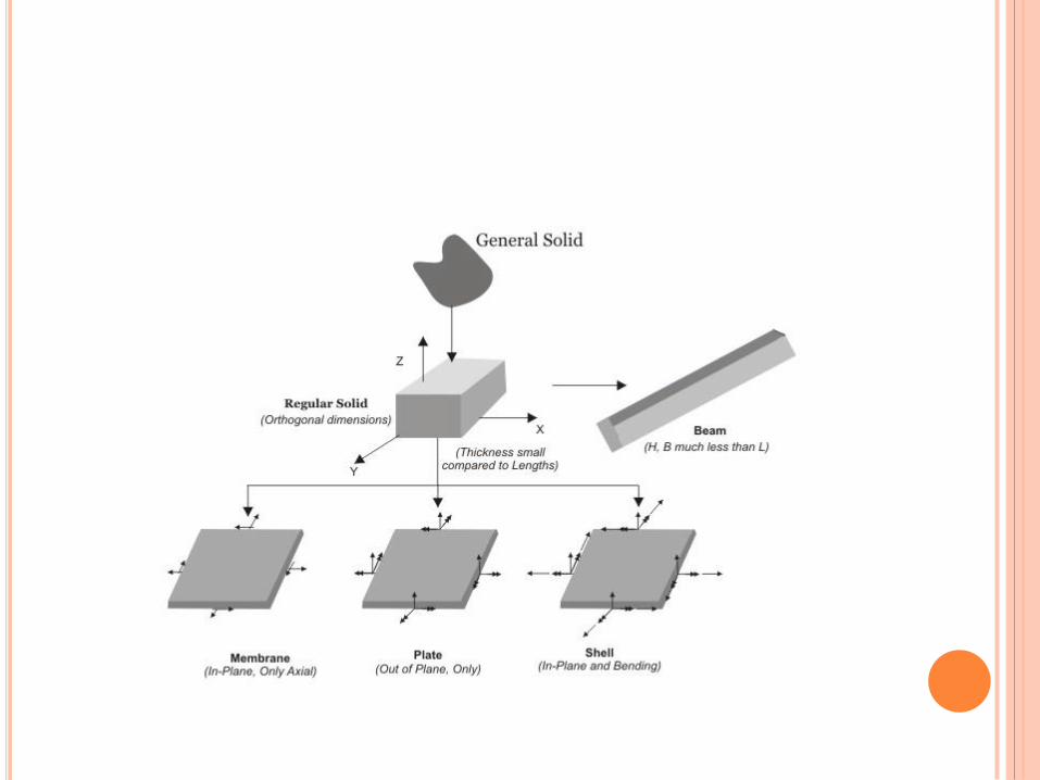
The elements may be 1D elements, 2D elements or 3D elements. The physical object can be modelled by
choosing appropriate element such as frame element, plate element, shell element, solid element, etc. All
elements are then assembled to obtain the solution of the entire domain/structure under certain loading
conditions. Nodes are assigned at a certain density throughout the continuum depending on the anticipated
stress levels of a particular domain. Regions which will receive large amounts of stress variation usually
have a higher node density than those which experience little or no stress.

Degrees of Freedom
A structure can have infinite number of displacements. Approximation with a reasonable level of
accuracy can be achieved by assuming a limited number of displacements. This finite number of
displacements is the number of degrees of freedom of the structure. For example, the truss
member will undergo only axial deformation. Therefore, the degrees of freedom of a truss
member with respect to its own coordinate system will be one at each node. If a two dimension
structure is modelled by truss elements, then the deformation with respect to structural coordinate
system will be two and therefore degrees of freedom will also become two.


NODES,
ELEMENTS,
NUMBERING,
NODAL CO-ORDINATE,
MEMBER
CONNECTIVITY DATA
.
(x,y,z)

xj-xi
yj-yi
i
j
(xi,yi)
(xj , yj )
22 )()( ijij yyxxL
CosCx L
) ( ij xx Sin yC
L
) (y ij y ;

(xi,yi,zi)
(xj , yj , zj)
222 )()()( ijijij zzyyxxL
xCL
) ( ij xx yCL
) (y ij y
zCL
) (z ij z

Percentage error in the measurement of perimeter of circle (D=1)
Sl.No.
No. of lines
Measured Length
Exact Perimeter
% Error
1.
3
L=2.5980762
3.141592654
17.30
2.
4
L=2.8284271
9.97
3.
6
L=3.0
4.517
4.
12
L=3.1058585
1.13
5.
24
L=3.1326286
0.285
6.
36
L=3.1376067
0.1268
7.
72
L=3.1405959
0.03173
8.
360
L=3.1415528
0.001269
1
2
3
4
5
6
1 2
3
4
5
6 7
8
9
10
11
12
1
2 5
4 3
6

24 NODES /
24 LINE ELEMENTS
48 NODES /
48 LINE ELEMENTS
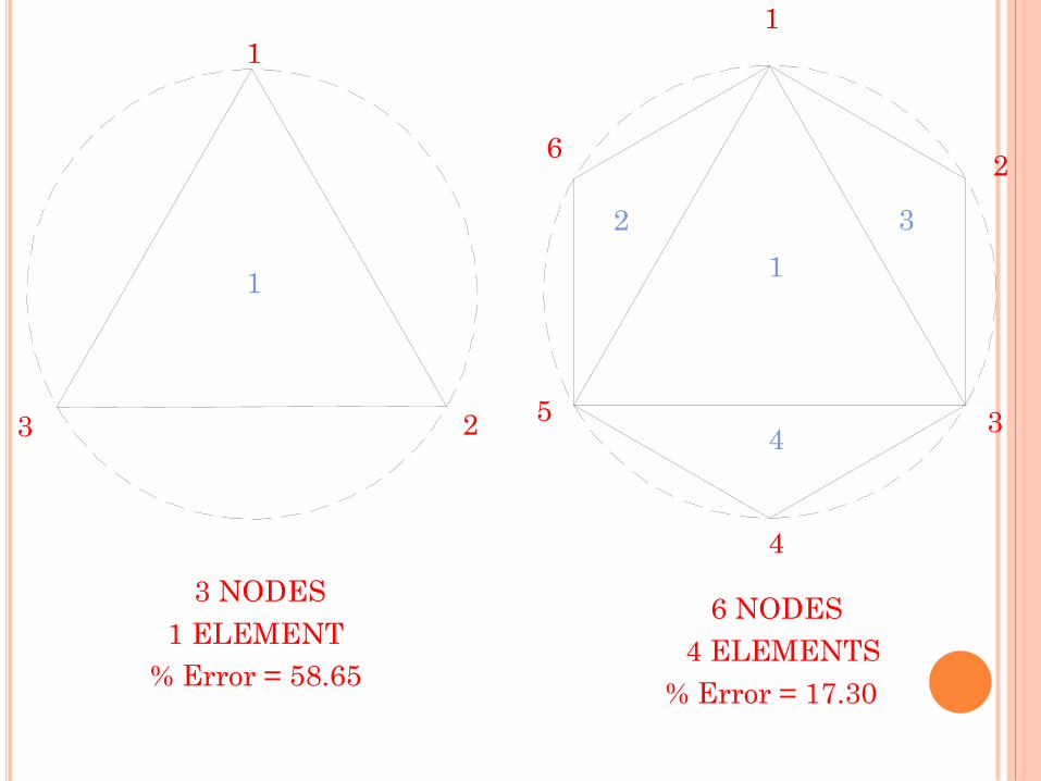
6 NODES
4 ELEMENTS
% Error = 17.30
1
3 2
4
1
2
3
4
5
6
3 NODES
1 ELEMENT % Error = 58.65
1
1
3 2
Percentage error in the measurement of area of circle
10
4
1
2 3
5
6 7
8
9 10
1 2
3
4
5
6
7 8
9
11
12
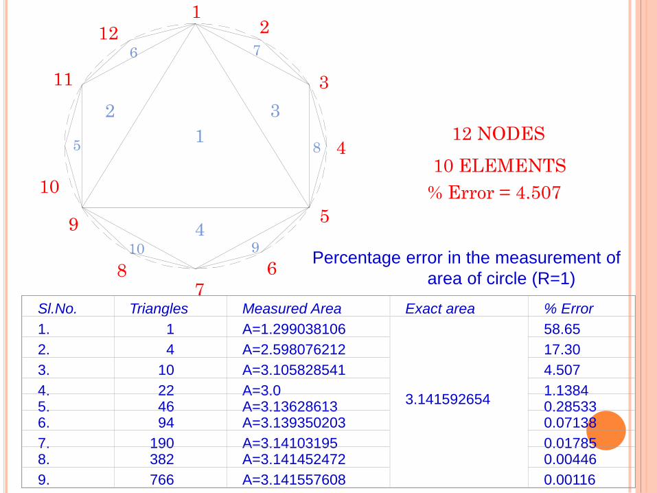
Percentage error in the measurement of
area of circle (R=1)
Sl.No.
Triangles
Measured Area
Exact area
% Error
1.
1
A=1.299038106
3.141592654
58.65
2.
4
A=2.598076212
17.30
3.
10
A=3.105828541
4.507
4.
22
A=3.0
1.1384
5.
46
A=3.13628613
0.28533
6.
94
A=3.139350203
0.07138
7.
190
A=3.14103195
0.01785
8.
382
A=3.141452472
0.00446
9.
766
A=3.141557608
0.00116
12 NODES
10 ELEMENTS
% Error = 4.507

. 10 . 11 . 12
. 7 . 8 . 9
. 4 . 5 . 6
. 1 . 2 . 3
1
2
3
4
5
6
7
8
9
10 11
12 13
14 15
PLANE FRAME-I
4.0m 4.0m
3.0m
3.0m
3.0m
NODE No.
NODAL CO-ORDINATES
NODE No.
NODAL CO-ORDINATES
01
0.0
0.0
07
0.0
6.0
02
4.0
0.0
08
4.0
6.0
03
8.0
0.0
09
8.0
6.0
04
0.0
3.0
10
0.0
9.0
05
4.0
3.0
11
4.0
9.0
06
8.0
3.0
12
8.0
9.0

. 10 . 11 . 12
. 7 . 8 . 9
. 4 . 5 . 6
. 1 . 2 . 3
1
2
3
4
5
6
7
8
9
10 11
12 13
14 15
PLANE FRAME-I
ELEMENT No.
NODAL CONNECTIVITY DATA
ELEMENT No.
NODAL CONNECTIVITY DATA
01
1
4
10
4
5
02
4
7
11
5
6
03
7
10
12
7
8
04
2
5
13
8
9
05
5
8
14
10
11
06
8
11
15
11
12
07
3
6
BOUNDARY CONDITIONS:1,2,3,4,5,6,7,8,9
08
6
9
09
9
12

1 2 3 4
5 6 7
8 9 10 11 12 13 14 15
.2 .4 .6 .8
.1 .3 .5 .7 .9
NODE No.
NODAL CO-ORDINATES
01
0.0
0.0
02
2.0
3.0
03
4.0
0.0
04
6.0
3.0
05
8.0
0.0
06
10.0
3.0
07
12.0
0.0
08
14.0
3.0
09
16.0
0.0
4.0 m
3.0m
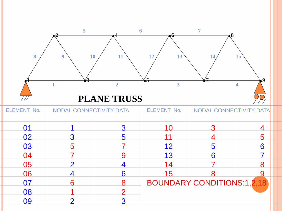
PLANE TRUSS
.2 .4 .6 .8
.1 .3 .5 .7 .9
1 2 3 4
5 6 7
8 9 10 11 12 13 14 15
PLANE TRUSS ELEMENT No.
NODAL CONNECTIVITY DATA
ELEMENT No.
NODAL CONNECTIVITY DATA
01
1
3
10
3
4
02
3
5
11
4
5
03
5
7
12
5
6
04
7
9
13
6
7
05
2
4
14
7
8
06
4
6
15
8
9
07
6
8
BOUNDARY CONDITIONS:1,2,18
08
1
2
09
2
3

1 2
3
4
1 2 4
3
n=1 i and j are the 2 d.o.f.
1 2 3 4
8 9 10 11 12 13 14 15
2*NODE NUMBER-1, 2*NODE NUMBER
1,2
3,4
5,6
7,8
9,10
11,12
13,14
15,16
17,18
.2 .4 .6 .8
.1 .3 .5 .7 .9


1
2
3
4
5
6
7
8
9
12
10 11
13 14
. 3 . 6 . 9 . 12
. 2 . 5 . 8 . 11
. 1 . 4 . 7 . 10
1,2,3
4,5,6
7,8,9
10,11,12
13,14,15
16,17,18
19,20,21
22,23,24
25,26,27
34,35,36
31,32,33
28,29,30

MINIMUM POTENTIAL ENERGY THEOREM

The principle of Minimum Potential Energy (MPE)
Deformation and stress analysis of structural systems can be accomplished
using the principle of Minimum Potential Energy (MPE), which states that
For conservative structural systems, of all the kinematically admissible
deformations, those corresponding to the equilibrium state extremize (i.e.,
minimize or maximize) the total potential energy. If the extremum is a
minimum, the equilibrium state is stable. Let us first understand what each
term in the above statement means and then explain how this principle is
useful to us.
A constrained structural system, i.e., a structure that is fixed at some
portions, will deform when forces are applied on it. Deformation of a
structural system refers to the incremental change to the new deformed
state from the original undeformed state. The deformation is the principal
unknown in structural analysis as the strains depend upon the deformation,
and the stresses are in turn dependent on the strains. Therefore, our sole
objective is to determine the deformation. The deformed state a structure
attains upon the application of forces is the equilibrium state of a structural
system. The Potential energy (PE) of a structural system is defined as the
sum of the strain energy (SE) and the work potential (WP).
PE = SE +WP

The strain energy is the elastic energy stored in deformed structure. It is
computed by integrating the strain energy density (i.e., strain energy per
unit volume) over the entire volume of the structure.
The work potential WP, is the negative of the work done by the external forces
acting on the structure. Work done by the external forces is simply the forces
multiplied by the displacements at the points of application of forces. Thus,
given a deformation of a structure, if we can write down the strains and stresses,
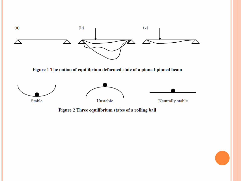
we can obtain SE, WP, and finally PE. For a structure, many deformations are
possible. For instance, consider the pinned-pinned beam shown in Figure 1a. It
can attain many deformed states as shown in Figure 1b. But, for a given force it
will only attain a unique deformation to achieve equilibrium as shown in Figure
1c. What the principle of MPE implies is that this unique deformation
corresponds to the extremum value of the MPE. In other words, in order to
determine the equilibrium deformation, we have to extremize the PE. The
extremum can be either a minimum or a maximum. When it is a minimum, the
equilibrium state is said to be stable. The other two cases are shown in Figure 2
with the help of the classic example of a rolling ball on a surface.

PROBLEMS
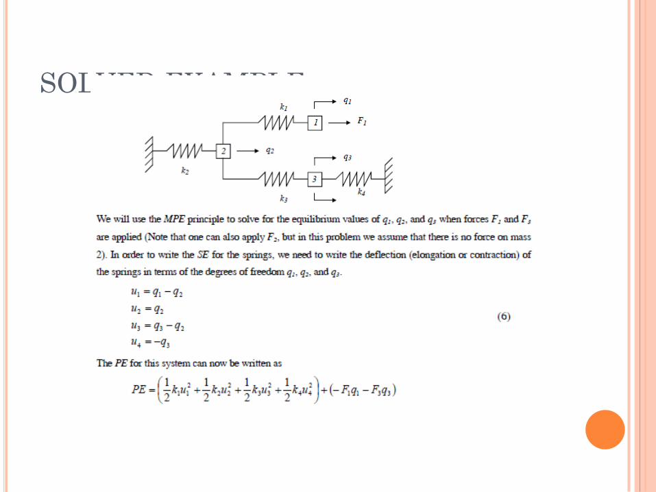
SOLVED EXAMPLE


TUTORIAL

MERITS AND DE-
MERITS

ADVANTAGES OF FEA
1. The physical properties, which complex for any closed bound solution, can be analyzed by this method.
2. It can take care of any geometry (may be regular or irregular).
3. It can take care of any boundary conditions.
4. Material anisotropy and non-homogeneity can be catered without much difficulty.
5. It can take care of any type of loading conditions.
6. This method is superior to other approximate methods like Galerkine and Rayleigh-Ritz
methods.
7. In this method approximations are confined to small sub domains.
8. In this method, the admissible functions are valid over the simple domain and have nothing to do with boundary, however simple or complex it may be.
9. Enable to computer programming.

DISADVANTAGES OF FEA
1. Computational time involved in the solution of the problem is high.
3. Proper engineering judgment is to be exercised to interpret results.
4. It requires large computer memory and computational time to obtain intend results.
5. There are certain categories of problems where other methods are more effective,
e.g., fluid problems having boundaries at infinity are better treated by the boundary
element method.
6. For some problems, there may be a considerable amount of input data. Errors may
creep up in their preparation and the results thus obtained may also appear to be
acceptable which indicates deceptive state of affairs. It is always desirable to make a
visual check of the input data.
7. In the FEM, many problems lead to round-off errors. Computer works with a limited
number of digits and solving the problem with restricted number of digits may not yield
the desired degree of accuracy or it may give total erroneous results in some cases. For
many problems the increase in the number of digits for the purpose of calculation
improves the accuracy.
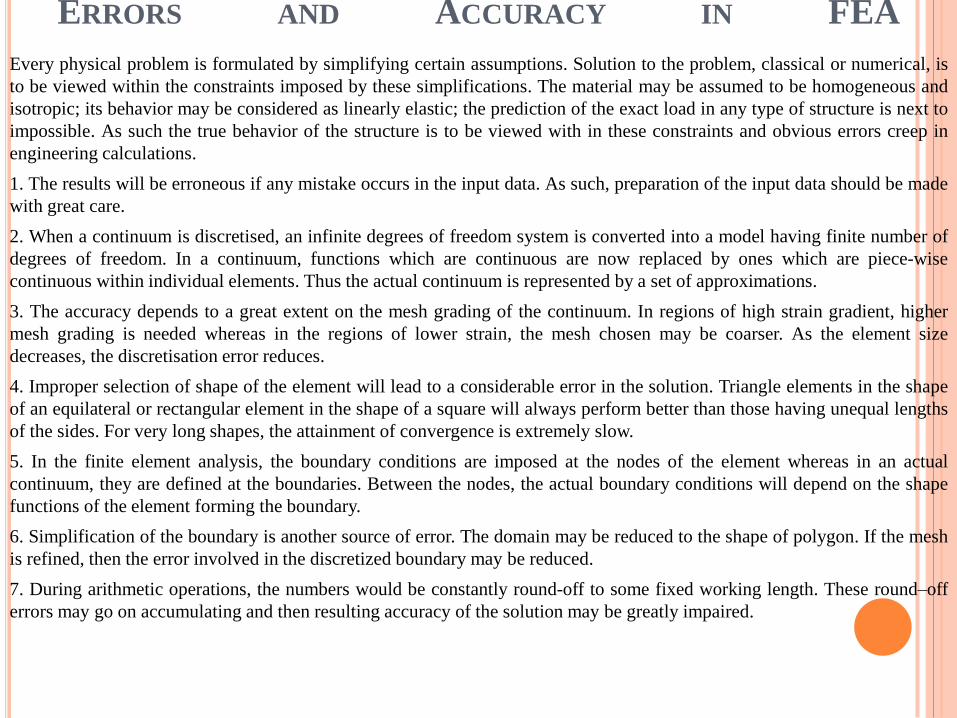
ERRORS AND ACCURACY IN FEA
Every physical problem is formulated by simplifying certain assumptions. Solution to the problem, classical or numerical, is
to be viewed within the constraints imposed by these simplifications. The material may be assumed to be homogeneous and
isotropic; its behavior may be considered as linearly elastic; the prediction of the exact load in any type of structure is next to
impossible. As such the true behavior of the structure is to be viewed with in these constraints and obvious errors creep in
engineering calculations.
1. The results will be erroneous if any mistake occurs in the input data. As such, preparation of the input data should be made
with great care.
2. When a continuum is discretised, an infinite degrees of freedom system is converted into a model having finite number of
degrees of freedom. In a continuum, functions which are continuous are now replaced by ones which are piece-wise
continuous within individual elements. Thus the actual continuum is represented by a set of approximations.
3. The accuracy depends to a great extent on the mesh grading of the continuum. In regions of high strain gradient, higher
mesh grading is needed whereas in the regions of lower strain, the mesh chosen may be coarser. As the element size
decreases, the discretisation error reduces.
4. Improper selection of shape of the element will lead to a considerable error in the solution. Triangle elements in the shape
of an equilateral or rectangular element in the shape of a square will always perform better than those having unequal lengths
of the sides. For very long shapes, the attainment of convergence is extremely slow.
5. In the finite element analysis, the boundary conditions are imposed at the nodes of the element whereas in an actual
continuum, they are defined at the boundaries. Between the nodes, the actual boundary conditions will depend on the shape
functions of the element forming the boundary.
6. Simplification of the boundary is another source of error. The domain may be reduced to the shape of polygon. If the mesh
is refined, then the error involved in the discretized boundary may be reduced.
7. During arithmetic operations, the numbers would be constantly round-off to some fixed working length. These round–off
errors may go on accumulating and then resulting accuracy of the solution may be greatly impaired.

STEPS IN
FEM
GENERAL PROCEDURE OF FINITE ELEMENT
ANALYSIS
The following steps are involved in the finite element analysis.
1. Discretization of the structure/continuum.
2. Choosing appropriate displacement function.
3. Strain-displacement matrix [B]
4. Stress-Strain matrix [D]
5. Development of element stiffness matrix.
6. Development of Load vector
7. Solution for the unknown displacements
8. Computation of the element strains and stresses/stress
resultants from the nodal displacement

1. Discretization of the structure/continuum.

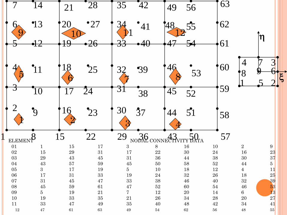
DISCRETIZATION OF TECHNIQUE The need of finite element analysis arises when the structural system in terms of its either
geometry, material properties, boundary conditions or loadings is complex in nature. For such
case, the whole structure needs to be subdivided into smaller elements. The whole structure is then
analyzed by the assemblage of all elements representing the complete structure including its all
properties. The subdivision process is an important task in finite element analysis and requires
some skill and knowledge. In this procedure, first, the number, shape, size and configuration of
elements have to be decided in such a manner that the real structure is simulated as closely as
possible. The discretization is to be in such that the results converge to the true solution. However,
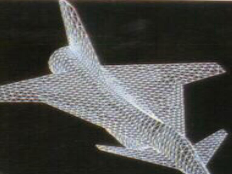
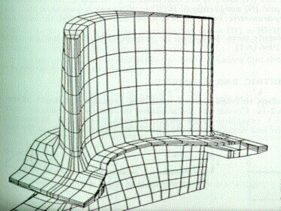
too fine mesh will lead to extra computational effort. Fig. 1.2.2 shows a finite element mesh of a
continuum using triangular and quadrilateral elements. The assemblage of triangular elements in
this case shows better representation of the continuum. The discretization process also shows that
the more accurate representation is possible if the body is further subdivided into some finer
mesh.

If the body is two dimensional or 3-D continuum divide the
continuum into finite number of elements
- by straight or curved lines in the case of 2-D
problem
- by straight or curved surfaces in the case of 3-D
problem.
Divide the elements into
triangles/rectangles/quadrilateral/3-D
elements based on the type of structure to be analysed.
All the elements are interconnected at some points called
as nodal points or nodes.

1 2 3 4
5
9 10 11 12
8 7 6
1 2 3 4 5
6 7 8 9 10
11 12 13 14 15
16 17 18 19 20

46 47 48 49 50 51 52 53 54
33 34 35 36 37 38 39 40
37 38 39 40 41 42 43 44 45
25 26 27 28 29 30 31 32
28 29 30 31 32 33 34 35 36
17 18 19 20 21 22 23 24
19 20 21 22 23 24 25 26 27
9 10 11 12 13 14 15 16
10 11 12 13 14 15 16 17 18
1 2 3 4 5 6 7 8
1 2 3 4 5 6 7 8 9

6 12 18 24 30 36 42 48 54
33 34 35 36 37 38 39 40
5 11 17 23 29 35 41 47 53
25 26 27 28 29 30 31 32
4 10 16 22 28 34 40 46 52
17 18 19 20 21 22 23 24
3 9 15 21 27 33 39 45 51
9 10 11 12 13 14 15 16
2 8 14 20 26 32 38 44 50
1 2 3 4 5 6 7 8
1 7 13 19 25 31 37 43 49

6
3
4 7 10
13
12
9
11
15
16
14 8
2
1
5

1
2
3
4
5
6
7
8
9
10
11
1
13
14
15
16
17
18
19
20
4.0
3.0
ELEMENT NODAL CONNECTIVITY DATA
no.
01 1 5 6 2
02 5 9 10 6
03 9 13 14 10
04 13 17 18 14
05 2 6 7 3
06 6 10 11 7
07 10 14 15 11
08 14 18 19 15
09 3 7 8 4
10 7 11 12 8
11 11 15 16 12
12 15 19 20 16
Joint co-ordinates
no. x y
01 0.0 0.0
02 0.0 1.0
03 0.0 2.0
04 0.0 3.0
05 1.0 0.0
06 1.0 1.0
07 1.0 2.0
08 1.0 3.0
09 2.0 0.0
10 2.0 1.0
11 2.0 2.0
12 2.0 3.0
13 3.0 0.0
14 3.0 1.0
15 3.0 2.0
16 3.0 3.0
17 4.0 0.0
18 4.0 1.0
19 4.0 2.0
20 4.0 3.0
2
3 4
1
5
9
2
6
10
3
7
11
4
8
12 12


3
7
2
4
6
5
8
9
10
11
12
13
14
15
16
17
18
19
20
21
22
23
24
25
26
27
28
29
30
31
32
33
34
35
36
37
38
39
40
41
42
43
44
45
46
47
48
49
50
51
1
12 11 10 9
8 7 6 5
4 3 2
1
ELEMENT no. NODAL CONNECTIVITY DATA
01 1 12 14 3 8 13 9 2
02 12 23 25 14 19 24 20 13
03 23 34 36 25 30 35 31 24
04 34 45 47 36 41 46 42 35
05 3 14 16 5 9 15 10 4
06 14 25 27 16 20 26 21 15
07 25 36 38 27 31 37 32 26
08 36 47 49 38 42 48 43 37
09 5 16 18 7 10 17 11 6
10 16 27 29 18 21 28 22 17
11 27 38 40 29 32 39 33 28
12 38 49 51 40 43 50 44 39
1 2
3 4
5
6 7
8
1
1
3
7
2
4
6
5
8
9
10
11
12
13
14
15
16
17
18
19
20
21
22
23
24
25
26
27
28
29
30
31
32
33
34
35
36
37
38
39
40
41
42
43
44
45
46
47
48
49
50
51
52
53
54
55
56
57
58
59
60
61
62
63
1
12 11 10 9
8 7 6 5
4 3 2
ELEMENT NODAL CONNECTIVITY DATA
01 1 15 17 3 8 16 10 2 9
02 15 29 31 17 22 30 24 16 23
03 29 43 45 31 36 44 38 30 37
04 43 57 59 45 50 58 52 44 5
05 3 17 19 5 10 18 12 4 11
06 17 31 33 19 24 32 26 18 25
07 31 45 47 33 38 46 40 32 39
08 45 59 61 47 52 60 54 46 53
09 5 19 21 7 12 20 14 6 13
10 19 33 35 21 26 34 28 20 27
11 33 47 49 35 40 48 42 34 41
12 47 61 63 49 54 62 56 48 55
1 2
3 4
5
6 7
8 9


2. Choosing appropriate displacement function.

2. Choice of displacement function:
Choose appropriate displacement function, which satisfy convergence and
compatability requirements. To satisfy convergence and compatability
requirements the displacement field must satisfy the following requirements.
The Finite element interpolations are characterised by the shape of the finite
element and order of approximations. In general the choice of a finite element
depends on the geometry of the global domain, the degree of accuracy required
in the solution, the ease of integration over the domain etc.
The global domain may be one, two and three dimensional.
Accordingly , the element is one, two and three dimensional.
A one dimensional element is simply a straight line. A two dimensional
element may be triangular, rectangular or quadrilateral and a three
dimensional element can be tetrahedron, a regular hexahedron or an irregular
hexahedron.
In general, the interpolation functions are the polynomials of various
degrees. They may also be given by the products of polynomials with
trigonometric or exponential functions.
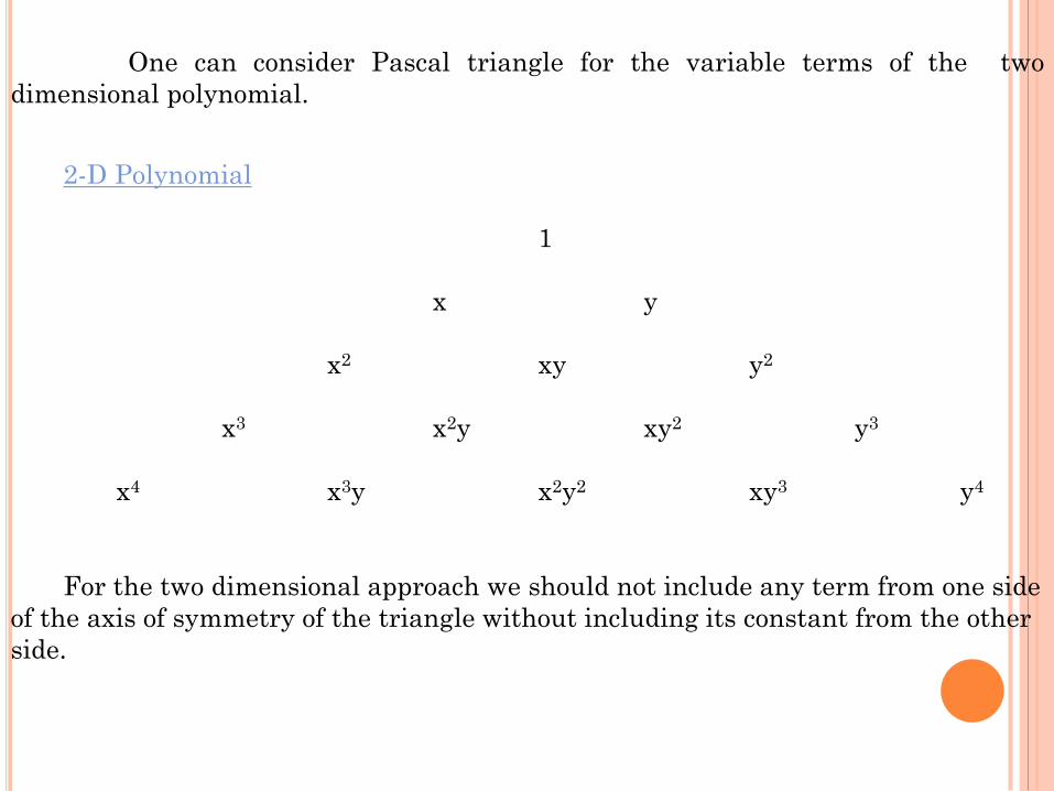
One can consider Pascal triangle for the variable terms of the two
dimensional polynomial.
2-D Polynomial
1
x y
x2 xy y2
x3 x2y xy2 y3
x4 x3y x2y2 xy3 y4
For the two dimensional approach we should not include any term from one side
of the axis of symmetry of the triangle without including its constant from the other
side.
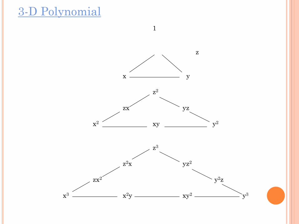
3-D Polynomial
1
z
x y
z2
zx yz
x2 xy y2
z3 z2x yz2
zx2 y2z
x3 x2y xy2 y3

PRINCIPLES OF ELASTICTY

EQUILIBRIUM EQUATIONS


STRAIN DISPLACEMENT RELATIONSHIP

3.3. Strain-displacement matrix [B]
The relation between strain and displacement is a key ingredient in
the finite element formulations. Displacements u,v and w are the
displacements along x,y and z directions respectively. x,y and z are the
rotations along x,y and z directions respectively.
By differentiating displacement function, Strain – displacement
matrix [B] can be obtained.
x = u = u,x y = v = v,y z = w = w,z
x y z
are the normal strains and
xy = u + v = u,y+v,x yz = v +w = v,z+ w,y zx = w + u = w,x+u,z
y x z y x z
are the shear strains.

The strain-displacement relations can be stated in matrix form asfollows.
x 0 0
x
y 0 0
y u
z 0 0
= z v
xy 0
y x w
yz 0
z y
zx 0
z x
{} = [B] {D*}
where [B] is the strain-displacement matrix.

CONSTITUTIVE RELATIONS
FOR
PLANE STRESS, PLANE STRAIN and
AXI-SYMMETRIC PROBLEMS

Stress –Strain relations:
For an isotropic material, we have only two independent elastic
constants and the generalized Hooke’s Law gives the following stress –
strain relations.
x = 1/E [ x - y -z] xy = xy / G
y = 1/E [-x + y -z] yz = yz / G
z = 1/E [-x - y+ z] zx = zx / G (2.2)

Axial element: Stress = Young’s modulus of Elasticity
Strain
/ = E {} = [E]{}
Elasticity matrix [D] = [E]
Plane Stress: If a thin plate is loaded by forces applied at the boundary,
the stress components z, xz and yz are zero on both faces of the plate, then the
state of stress is called plane stress.
For plane stress case the basic equations become
x = 1/E [x - y]
y = 1/E [-x + y] (2.2.2)
xy = xy / G
(I) + * (II) x + y = 1/E [x - 2x] = x (1-2)/E.
x = E [x + y]
(1-2)


Plane Strain: When the length of the member in the z direction in either
very large so that no displacement is possible or the movements along the z-axis
are otherwise prevented so that z = yz = zx = 0 then the state of strain is said
to be plane strain.
z = 0 = 1/E [- x - y + z] = 0
z = (x + y).
whereas y = E [x + y]
(1-2)
xy = G xy = E xy
2(1+)
In a matrix form
x E 1 0 x
y = ----- 1 0 y
xy 1-2 0 0 1- xy
2


Substituting in Eqs. (2.2)
x = 1/E [x - y - 2 (x + y)]
= 1/E [(1-2) x - (1+) y] = (1+) [(1-)x - y]
E
where as : y = (1+) [-x + (1-)y]
E
(1-)x + y = (1+) [(1-)2 x - 2x] = (1+)(1-2) x
E E
x = E [(1-)x + y]
(1+)(1-2)
where by y = E [x + (1-)y]
(1+)(1-2)
xy = G xy = E .xy
2(1+)

So, Stress-Strain matrix for plane strain case is
x 1- 0 x
y = E 1- 0 y
xy (1+)(1-2) 0 0 1-2 xy
2
{} = [D]{}

3.4. Stress-strain relations:
We symbolize stress-strain relations as
x (1-) 0 0 0 x
y = E (1-) 0 0 0 y
z (1+)(1-2) (1-) 0 0 0 z
xy 0 0 0 (1-2 )/2 0 0 xy
yz 0 0 0 0 (1-2 )/2 0 yz
zx 0 0 0 0 0 (1-2 )/2 zx
where E/G = 2(1+)

Axial element: Stress = Young’s modulus of Elasticity
Strain
/ = E {} = [E]{}
Elasticity matrix [D] = [E]
Plane Stress: If a thin plate is loaded by forces applied at the boundary,
the stress components z, xz and yz are zero on both faces of the plate, then the
state of stress is called plane stress.
x E 1 0 x
y = ----- 1 0 y
xy 1-2 0 0 1- xy
2

Plane Strain: When the length of the member in the z direction in either
very large so that no displacement is possible or the movements along the z-axis
are otherwise prevented so that z = yz = zx = 0 then the state of strain is said
to be plane strain.
z = 0 = 1/E [- x - y + z] = 0
z = (x + y).
So, Stress-Strain matrix for plane strain case is
x 1- 0 x
y = E 1- 0 y
xy (1+)(1-2) 0 0 1-2 xy
2
{} = [D]{}

Axi- Symmetric Problems

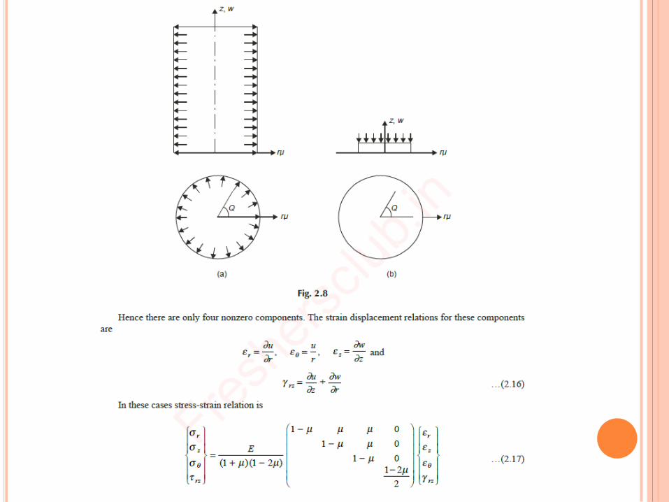

5. Development of element stiffness matrix.
6. Development of Load vector
7. Solution for the unknown displacements
8. Computation of the element strains and
stresses/stress resultants from the nodal
displacement

3.5. Stiffness Matrix:
Element stiffness matrix can be developed using the following
formulae: [K*] = [B]T [D][B] dv
The element stiffness matrices of individual elements are to be assembled
through a proper numbering system so as to reduce the size of the structure stiffness
matrix. The element stiffness matrices are to be assembled by superposing the nodal
components of stiffnesses of elements at each and every node.
3.6 Load Vector:
Load vector of an element subjected to initial stress,strain, surface
loads, body loads and concentrated loads is
{Q*} = ( -[B]T [0] dv + [B]
T [D] {0} + [N]
T {w}dx
+ [N] T
{q} ds + [N] T
{F} dv ) + {P*} (3.6)

3.7. Solution of the final set of simultaneous equations:
The structure stiffness matrix is to be modified to impose boundary
conditions that allows prescribed degrees of freedom to be either zero or
non zero. Structural equations
[K] {D} = {Q} can be solved by making use of algorithms available for the
solution of simultaneous equations. Finally, unknown nodal displacements
are computed.
3.8. Stress Computation:
After solving nodal displacements, all nodal degrees of freedom of
the structure are known. Finally, stresses are computed from strains in
individual elements by using the following equations.
{} = [B]{D*}
{} = [D]{ } = [D][B]{D*}