unit 12: correlation - annenberg learner - teacher ... · pdf fileresearchers about the...
TRANSCRIPT

Unit 12: Correlation | Student Guide | Page 1
Unit 12: Correlation
Summary of VideoHow much are identical twins alike – and are these similarities due to genetics or to the environment in which the twins were raised? The Minnesota Twin Study, a classic correlation study on genes versus environment done in the 1980s, studied subjects like Jerry Levey and Mark Newman, identical twins raised apart. The two looked alike, were both involved with volunteer fire departments, and even had the same beer preference. Given they were separated at birth, the measure of correlation or similarity between them should be attributed to genetics. Contrast this with correlations between identical twins raised together. Here the similarities ought to be due to common family environment in addition to common genes. The difference between the size of the correlation between these two groups of twins tells researchers about the influence of the common family environment.
So how do you assess the size of the correlation? We can often get a pretty good idea simply by looking at a scatterplot of the data. Take, for example, Figure 12.1, a scatterplot of heights of pairs of twins who have been raised apart.
Figure 12.1. Scatterplot of heights.

Unit 12: Correlation | Student Guide | Page 2
We can quickly see that the taller one twin of a pair is, the taller is the other; there is a positive correlation between the two. The pattern appears quite strong, which is not surprising for a physical trait. But would we also find correlations between behavioral traits? Figure 12.2 shows a scatterplot of a personality inventory study given to pairs of identical twins raised apart.
Figure 12.2. Scatterplot of personality inventory.
While the relationship is not as clear as it was for height, the points do tend to increase together. Remember, the twins were raised in different families so the fact that a correlation exists at all can only be attributed to their common genes. We can compare these two scatterplots more objectively with a direct measure of correlation denoted as r. The formula for calculating r is given below.
r = 1n −1
x − xsx
⎛
⎝⎜⎞
⎠⎟∑ y − y
sy
⎛
⎝⎜
⎞
⎠⎟
However, in practice, most people use software or a calculator that finds r from the keyed in data on x and y.
The value of r is always a number between –1 and 1; positive r means positive association, and the closer r is to 1, the closer to a straight line the scatterplot is; r = +1 is perfect positive linear association, in which case all the points lie exactly on a straight line that has
Unit 12: Correlation | Student Guide | Page 3
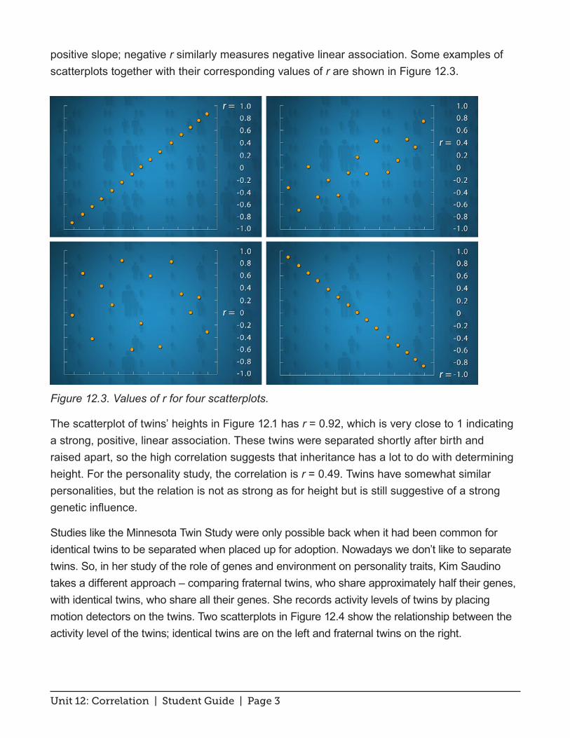
positive slope; negative r similarly measures negative linear association. Some examples of scatterplots together with their corresponding values of r are shown in Figure 12.3.
Figure 12.3. Values of r for four scatterplots.
The scatterplot of twins’ heights in Figure 12.1 has r = 0.92, which is very close to 1 indicating a strong, positive, linear association. These twins were separated shortly after birth and raised apart, so the high correlation suggests that inheritance has a lot to do with determining height. For the personality study, the correlation is r = 0.49. Twins have somewhat similar personalities, but the relation is not as strong as for height but is still suggestive of a strong genetic influence.
Studies like the Minnesota Twin Study were only possible back when it had been common for identical twins to be separated when placed up for adoption. Nowadays we don’t like to separate twins. So, in her study of the role of genes and environment on personality traits, Kim Saudino takes a different approach – comparing fraternal twins, who share approximately half their genes, with identical twins, who share all their genes. She records activity levels of twins by placing motion detectors on the twins. Two scatterplots in Figure 12.4 show the relationship between the activity level of the twins; identical twins are on the left and fraternal twins on the right.

Unit 12: Correlation | Student Guide | Page 4
Figure 12.4. Activity levels of identical and fraternal twins in laboratory setting.
As expected, the correlation for the identical twins, r = 0.48, is higher than the correlation for fraternal twins, r = 0.26. Since the environments these toddlers were raised in were the same, the difference in correlations can only be accounted for by the genes they inherited. But that’s not the end of the story. These data were collected in a laboratory environment. Next, the researcher collected the same type of data on the twins in their home environment. In the home setting, the difference in the correlations largely disappeared – for the identical twins, r = 0.87, and for the fraternal twins, r = 0.70. The conclusion: it looks as if twins’ behavioral patterns are governed both by genes and by environment.

Unit 12: Correlation | Student Guide | Page 5
Student Learning Objectives
A. Recognize the correlation coefficient r as a measure of the strength and direction of a linear relationship between two quantitative variables.
B. Be aware of the basic properties of r:
• The sign of r shows positive or negative association. • The value of r always satisfies −1≤ r ≤1. • The value of r remains the same when the two variables are interchanged and also
when the units of the variables are changed. • The value of r moves away from 0 toward -1 or 1 as the scatterplot points show a
closer straight-line pattern; 1r = ± means a perfect straight-line relation.
C. Be able to use the formula to calculate r from small data sets, say 5 observations; be able to use technology to calculate r for larger data sets.
D. Understand that a strong correlation can have various interpretations and that correlation does not imply causation.
E. Understand the importance of looking at a scatterplot of the data when using r to interpret the strength of a linear relationship. Know that a single outlier can have a dramatic effect on the value of r.

Unit 12: Correlation | Student Guide | Page 6
Content Overview
Correlation is the usual measure of association between two quantitative variables. More specifically, Pearson’s product moment correlation coefficient r, or the correlation coefficient for short, measures the strength and direction of linear (straight-line) relationships. Given a linear relationship exists between two quantitative variables, r is positive if the data fall about a line that has a positive slope and r is negative if the data fall about a line that has a negative slope. The value of r is always between -1 and 1. If r = -1, the data fall exactly on a line with negative slope and if r = 1, the data fall exactly on a line with positive slope. The correlation measures both the strength and direction of a linear relationship. Figure 12.5 provides some guidelines:
Figure 12.5. Using r to measure the strength and direction of a linear relationship.
There are a variety of formulas that can be used to compute r, but all are algebraically equivalent to the one given below.
Formula for Calculating r
Graphing calculators, spreadsheets, and statistical computing packages compute r very efficiently. So, unless the size of the data set is quite small, it is best to use technology to compute the value of r. However, the formula in the form presented above does provide the following insight:
• Notice that r consists of the product of z-scores for the x and y values. Therefore, the correlation coefficient is unit-free because units associated with the x and y
-1.0 -0.8 -0.5 0.0 0.5 1.00.8
Stro
ng
Stro
ng
Mod
erat
e
Mod
erat
e
Wea
k
Wea
k
Negative Positive
r = 1n −1
x − xsx
⎛
⎝⎜⎞
⎠⎟∑ y − y
sy
⎛
⎝⎜
⎞
⎠⎟
Unit 12: Correlation | Student Guide | Page 7
values cancel out. If we change the units of our data, for example change inches to centimeters, the value of r will remain the same.
• Interchanging x and y does not affect r.
• If we add a constant to all data values, either the x’s or y’s, the value of r does not change. If we multiple all data values, either the x’s or y’s, by a constant, the value of r does not change.
Always make a scatterplot of the data before interpreting correlation. A single extreme outlier added to data that otherwise has a positive association can result in a negative correlation. A strong relationship that happens to be curved can produce a value of r close to 0. So, always check to see that a scatterplot of the data has linear form and is free of extreme outliers before using correlation to measure the strength of a relationship between two quantitative variables. In addition, it should be noted that a strong correlation does not always mean that there is a direct cause-and-effect link between the variables. Unit 14, The Question of Causation, looks at causation in detail.

Unit 12: Correlation | Student Guide | Page 8
Key Terms
Correlation, denoted by r, measures the direction and strength of a linear relationship between two quantitative variables. The formula for computing Pearson’s correlation coefficient is:
r = 1n −1
x − xsx
⎛
⎝⎜⎞
⎠⎟∑ y − y
sy
⎛
⎝⎜
⎞
⎠⎟

Unit 12: Correlation | Student Guide | Page 9
The Video
Take out a piece of paper and be ready to write down answers to these questions as you watch the video.
1. If it were true that two identical twins always had the same height, what would the scatterplot of the heights of several pairs of identical twins look like? What would be the correlation r between the heights?
2. What are all the possible values of the correlation coefficient r?
3. If heredity plays a strong role in determining personality, will the correlation between twins raised together be about the same as, or much larger than, the correlation between twins raised apart?
4. Is it easy to guess how large the correlation is by looking at a scatterplot? Explain.

Unit 12: Correlation | Student Guide | Page 10
Unit Activity: Scatterplots and Correlation
Pearson’s product moment correlation coefficient, r, measures the strength of a linear relationship. So, before computing r, make a scatterplot to check that the relationship between two variables has linear form. The value of r always lies between -1 and 1 and provides information both on a relationship’s direction (positive or negative association) and strength (closeness of data points to a line). In the questions that follow, use technology (graphing calculator, spreadsheet, statistical computing software) to compute r. You can either make the scatterplots by hand or use technology.
1. Enter the following data into two columns, one for x and the other for y.
Table 12.1. Data set A.
a. Make a scatterplot of y versus x. Does the pattern appear to be linear or nonlinear? Is the association between x and y positive or negative?
b. Calculate the correlation, r. What does this tell you about the pattern of dots in your scatterplot?
2. Repeat question 1 using Data set B from Table 12.2.
Table 12.2. Data set B.
3. In the next data sets, the scatter of the points is increased. Your task will be to see how the increase of scatter affects correlation.
x 8 11 5 2 4y 17 23 11 5 9
Table 12.1
x 10 3 5 1 6y -30 -2 -10 6 -14
Table 12.2
Unit 12: Correlation | Student Guide | Page 11
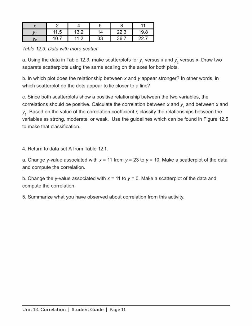
Table 12.3. Data with more scatter.
a. Using the data in Table 12.3, make scatterplots for y1 versus x and y
2 versus x. Draw two
separate scatterplots using the same scaling on the axes for both plots.
b. In which plot does the relationship between x and y appear stronger? In other words, in which scatterplot do the dots appear to lie closer to a line?
c. Since both scatterplots show a positive relationship between the two variables, the correlations should be positive. Calculate the correlation between x and y
1 and between x and
y2. Based on the value of the correlation coefficient r, classify the relationships between the
variables as strong, moderate, or weak. Use the guidelines which can be found in Figure 12.5 to make that classification.
4. Return to data set A from Table 12.1.
a. Change y-value associated with x = 11 from y = 23 to y = 10. Make a scatterplot of the data and compute the correlation.
b. Change the y-value associated with x = 11 to y = 0. Make a scatterplot of the data and compute the correlation.
5. Summarize what you have observed about correlation from this activity.
x 2 4 5 8 11y1 11.5 13.2 14 22.3 19.8y2 10.7 11.2 33 36.7 22.7
Table 12.3

Unit 12: Correlation | Student Guide | Page 12
Exercises
1. Archaeopteryx is an extinct beast having flight feathers like a bird but teeth and a long bony tail like a reptile. Only five complete fossil specimens are known. These specimens differ greatly in size, so some experts think they are different species. Others think they are individuals from the same species but of different ages. Correlation can help decide the question. If the specimens belong to the same species and differ in size because they are at different stages of growth, there should be a strong straight-line relationship between the lengths of a pair of bones from all individuals. Outliers from this relationship would suggest a different species. Table 12.4 gives the lengths in centimeters of the femur (a leg bone) and the humerus (a bone in the upper arm) for the five specimens.
Table 12.4. Bone lengths from fossils.
a. Make a scatterplot of the data in Table 12.4. Does the relationship appear linear? Is the association between femur length and humerus length positive or negative?
b. Calculate the correlation coefficient, r , using the formula.
c. Based on the value of r , do you conclude that these specimens are all from the same species? Explain.
2. Each of the following statements contains a blunder. Explain in each case what is wrong.
a. There is correlation r = 0.6 between the gender of students and their scores on a mathematics exam.
b. We found a high correlation (r = 1.09) between students’ scores on the math part of the SAT and their scores on the verbal part of the SAT.
c. The correlation between amount of fertilizer and yield of corn was found to be r = 0.23 bushel.
Femur (cm) 38 56 59 64 74 Humerus (cm) 41 63 70 72 84
Table 12.4

Unit 12: Correlation | Student Guide | Page 13
3. Foal weight at birth is one indicator of the newborn’s health. Is a mare’s (mother’s) weight related to the weight of her foal? Data on the weights of 15 mares and their foals appears in Table 12.5.
Table 12.5. Weight of mares and their newborn foals. Source: “Suckling behavior does not measure milk intake in horses, Equus caballus,” Careron, E. et al. (Animal
Behavior [1999]: p673 – 678).
a. Make a scatterplot of the data in Table 12.5. Which variable did you put on the horizontal axis. Explain your choice.
b. Based on your scatterplot, does the association between foal weight and mare weight appear to be positive, negative, or neither? Explain.
c. Based on your scatterplot, would you expect the correlation to be closer to -1, 0, or 1? Justify your choice.
d. Calculate the value of the correlation coefficient r. Does your result confirm or refute your answer to (c)?
Mare's Weight (kg) Foal's Weight (kg)
556 129.0638 119.0588 132.0550 123.5580 112.0642 113.5568 95.0642 104.0556 104.0616 93.5549 108.5504 95.0515 117.5551 128.0594 127.5
Table 12.5

Unit 12: Correlation | Student Guide | Page 14
4. Table 12.6 gives the average times by age (ages 18 – 50) for female runners in the 2012 Boston Marathon.
Table 12.6. Average time by age of female runners in 2012 Boston Marathon.
a. What is the correlation between runners’ average time and age? What does this tell you about the relationship between age and average time to run the race?
Age Average Time (min)18 28819 28620 26021 27422 27323 26524 27125 27226 27227 26528 26429 27030 26531 26832 26133 26534 26835 26036 26137 26438 27139 26440 26841 26942 27143 26644 26745 27346 28047 27648 27949 28250 281
Table 12.6

Unit 12: Correlation | Student Guide | Page 15
b. Make a scatterplot of average time versus age. Describe the relationship between these variables.
c. Explain why it is important to make a scatterplot of data before trying to interpret the value of the correlation coefficient r. Refer to your solutions to parts (a) and (b) as part of your answer.

Unit 12: Correlation | Student Guide | Page 16
Review Questions
1. A student wonders if people of similar heights tend to date each other. She measures herself and several of her friends. Then she measures the next man each woman dates. Table 12.7 contains the data collected by the student.
Table 12.7. Heights of women and their dates.
a. Make a scatterplot of these data. Based on the scatterplot, do you expect the correlation to be positive or negative? Near +1 or -1, or neither?
b. Find the correlation r between the heights of the men and women. (Unless instructed otherwise, feel free to use technology.) Based on this correlation would you classify the strength of the linear relationship as strong, moderate, or weak? Explain.
2. Return to the data from Table 12.7.
a. If every woman in the study dated a man exactly 3 inches taller than she is, what would be the correlation between male and female heights? Explain.
b. How would r change if all the men were 6 inches shorter than the heights given in Table 12.7? Does the correlation help answer the question of whether women tend to date men taller than themselves? Explain.
c. Change all the heights in Table 10.1 from inches to centimeters. (Recall 1 inch = 2.54 centimeters.) Recalculate the correlation using the heights data measured in centimeters. How did this conversion from inches to centimeters affect the value of r?
3. Some students are good in mathematics and others are better at reading or writing. The question is whether there is any relationship between a student’s ability in math and his/her ability in reading or writing. The SAT, a standardized test for college admissions that is widely used in the United States, has three sections, Math, Critical Reading, and Writing. Table 12.8 contains SAT Math, Writing, and Critical Reading test scores for 20 randomly chosen students accepted by a university.
Female Height (in) 66 64 66 65 70 65
Male Height (in) 72 68 70 68 71 65
Table 12.7

Unit 12: Correlation | Student Guide | Page 17
Table 12.8. SAT test scores from 20 students.
a. We are interested in the relationship between students’ scores on the SAT Math and their scores on the SAT Critical Reading and SAT Writing. Make two scatterplots, one of SAT Math versus SAT Critical Reading and the other of SAT Math versus SAT Writing. (In both scatterplots, SAT Math is being treated as the response variable.) Use the same scaling for both scatterplots. Based on your scatterplots, which variable has a stronger correlation with the SAT Math, the SAT Critical Reading or the SAT Writing? Explain.
b. Calculate the correlation between SAT Math scores and SAT Critical Reading scores. Then do the same for SAT Math scores and SAT Writing scores. Which variable, SAT Critical Reading or SAT Writing, is more highly correlated with SAT Math? Would you classify the strength of this relationship as strong, moderate, or weak?
Math Writing Critical Reading 440 410 410550 570 520520 520 540420 470 410550 620 530650 560 560610 620 550610 520 600340 470 400600 540 620680 580 580440 430 470440 450 370390 430 390460 600 600460 520 500520 570 580540 530 570420 430 470550 480 530
Table 12.8

Unit 13: Two-Way Tables | Student Guide | Page 1
Unit 13: Two-Way Tables
Summary of VideoThis video deals with analysis of categorical variables (for example, gender, race, occupation) and relationships between categorical variables. The context is a Happiness Survey that was part of Somerville, Massachusetts’ 2011 annual census. The video focuses on two of the survey questions, one that asks respondents to rate their current level of happiness and the other that asks them to rate the beauty of Somerville. Happiness ratings are boiled down into three categories: Unhappy, So-So, and Happy. Ratings of Somerville’s physical beauty are categorized as Bad, OK, and Good. Results from these two questions are organized into a two-way table with Happiness as the row variable and Physical Beauty as the column variable (see Table 13.1). The marginal totals (bottom row and right-most column) have been added to the two-way table.
Table 13.1. Results from rating happiness and Somerville’s physical beauty.
Notice that 5785 Somerville residents answered both of these questions. (The table only accounts for respondents who have answered both questions.) First, look at the distribution of each variable separately – this is called a marginal distribution. Computations of the marginal distributions of the two variables appear in Tables 13.2 and 13.3. From the marginal distributions we find that slightly more than 58% of respondents reported they were Happy and around 36% of the respondents rated Somerville’s physical beauty as Good.
See tables on next page...
Bad OK Good Total
Unhappy 90 123 62 275
So-so 555 972 610 2137
Happy 541 1426 1406 3373
1186 2521 2078 5785
Table 13.1
Physical Beauty
Happiness
Total

Unit 13: Two-Way Tables | Student Guide | Page 2
Table 13.2. Marginal distribution of Happiness.
Table 13.3. Marginal distribution of Physical Beauty.
Next, we dig even deeper into the two-way table’s data by computing conditional distributions, distributions of one variable restricted to a single outcome of another variable. For example, we can investigate how just the Unhappy people rated Somerville’s beauty. In this case, we are looking at the distribution of beauty ratings just within the Unhappy group (275 respondents). Here are the calculations:
Bad: 90/275 × 100% ≈ 32.73% OK: 123/275 × 100% ≈ 44.73% Good: 62/275 × 100% ≈ 22.55%
Table 13.4 shows the conditional distribution of Physical Beauty for each category of Happiness.
Table 13.4. Conditional distribution of Physical Beauty for each Happiness category.
Notice that only 22.55% of Unhappy people rated Somerville’s beauty as Good compared to 41.68% of the Happy people – clearly there is a connection between the Happiness and Physical Beauty variables. The graphic display in Figure 13.1 can help us visualize this linkage.
Bad OK GoodMarginal Distribution
1186/5785 × 100% ≈ 20.50%
2521/5785 × 100% ≈ 43.58%
2078/5785 × 100% ≈ 35.92%
Table 13.3
Physical Beauty
Bad OK Good
Unhappy 32.73% 44.73% 22.55% 100%
So-so 25.97% 45.48% 28.54% 100%
Happy 16.04% 42.28% 41.68% 100%
Table 13.4
Physical BeautyTotal
Happiness
Marginal Distribution
Unhappy 275/5785 × 100% ≈ 4.75%
So-so 2137/5785 × 100% ≈ 36.94%
Happy 3373/5785 × 100% ≈ 58.31%
Table 13.2
Happiness

Unit 13: Two-Way Tables | Student Guide | Page 3
Figure 13.1. Conditional distribution of Physical Beauty for each level of Happiness.
The bar graph in Figure 13.1 shows that as the level of Happiness goes up, the percentage of Bad ratings for Physical Beauty goes down. In addition, as the level of Happiness goes up, the level of Good beauty ratings also goes up. As we know, correlation isn’t necessarily causation. However, now that Somerville has identified a link between residents’ happiness levels and their thoughts on the city’s physical beauty, officials want to dig deeper on the next survey in an effort to improve residents’ satisfaction with Somerville.
Unit 13: Two-Way Tables | Student Guide | Page 4
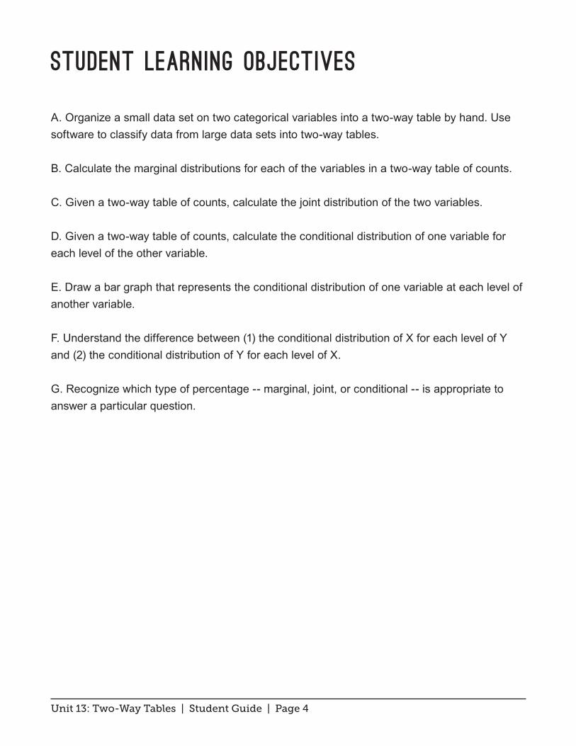
Student Learning Objectives
A. Organize a small data set on two categorical variables into a two-way table by hand. Use software to classify data from large data sets into two-way tables.
B. Calculate the marginal distributions for each of the variables in a two-way table of counts.
C. Given a two-way table of counts, calculate the joint distribution of the two variables.
D. Given a two-way table of counts, calculate the conditional distribution of one variable for each level of the other variable.
E. Draw a bar graph that represents the conditional distribution of one variable at each level of another variable.
F. Understand the difference between (1) the conditional distribution of X for each level of Y and (2) the conditional distribution of Y for each level of X.
G. Recognize which type of percentage -- marginal, joint, or conditional -- is appropriate to answer a particular question.

Unit 13: Two-Way Tables | Student Guide | Page 5
Content Overview
This unit discusses methods for studying relationships between two categorical variables. Some categorical variables – such as gender, eye color, occupation – are inherently categorical. Others – such as age in the following categories: under 30, between 30 and 60, and over 60 – are created by grouping values of a quantitative variable into categories. Nominal categorical variables have values with no inherent order; ordinal categorical variables have values with an inherent order. One example of an ordinal variable would be college class: freshman, sophomore, junior, and senior. Any table or graphic display involving an ordinal variable should preserve the inherent order of values for that variable.
A relationship between two categorical variables requires that both variables must be responses from the same individuals or cases. The first step in extracting information about a relationship between the two variables is to organize the raw data into a two-way table. Table 13.5 shows data from the first 10 respondents to Somerville’s Happiness Survey.
Table 13.5. Data on first 10 respondents to Happiness Survey.
For the two-way table, we’ll use Happiness as the row variable and Physical Beauty as the column variable (just as was done in the video). Respondents #1 and #2 replied Happy and Good to the questions on rating personal happiness and Somerville’s physical beauty, respectively. Hence, we have entered two tally marks into the corresponding cell of Table 13.6. Respondent #3 replied So-so and OK and we have entered a single tally mark into the corresponding cell of Table 13.6. Table 13.7 shows the results from the completed tally converted to numbers.
Survey ID Happiness Physical Beauty
1 Happy Good2 Happy Good3 So-so OK4 Happy Bad5 So-so Good6 Happy Good7 Unhappy Bad8 So-so Good9 So-so Bad
10 So-so OK
Table 13.5

Unit 13: Two-Way Tables | Student Guide | Page 6
Table 13.6. Making a two-way table from the data in Table 13.5.
Table 13.7. Two-way table for data in Table 13.5.
Although it’s good to practice making a two-way table by hand on a small data set, there were 5785 respondents to these two questions in the Somerville survey. Organizing large data sets into two-way tables is tedious to do by hand and best left to technology.
Once we have organized the data into a two-way table, we can compare different types of percentages. Next, we look at responses to a survey of 12th grade students. Table 13.8 organizes their responses to questions on gender and how many hours per week they work at either a paid or unpaid job. The row variable is Hours and the column variable is Gender. The row and column totals have been added to the table.
Table 13.8. Two-way table for Hours and Gender.
From the marginal totals, Table 13.8 shows 13 respondents who did not work and 21 respondents who were male. From the joint distribution, there were three respondents who fell into both of these categories, males who did not work.
Female Male Total
None 10 3 13
10 or fewer hours 7 4 11
11 to 20 hours 2 7 9
21 to 30 hours 8 3 11
More than 30 hours 2 4 6
Total 29 21 50
Table 13.8
Count
Gender
Hours
Bad OK Good Unhappy So-so | Happy ||
Table 13.6
Physical Beauty
Happiness
Bad OK Good Unhappy 1 0 0 So-so 1 2 2 Happy 1 0 3
Table 13.7
Physical Beauty
Happiness
Unit 13: Two-Way Tables | Student Guide | Page 7
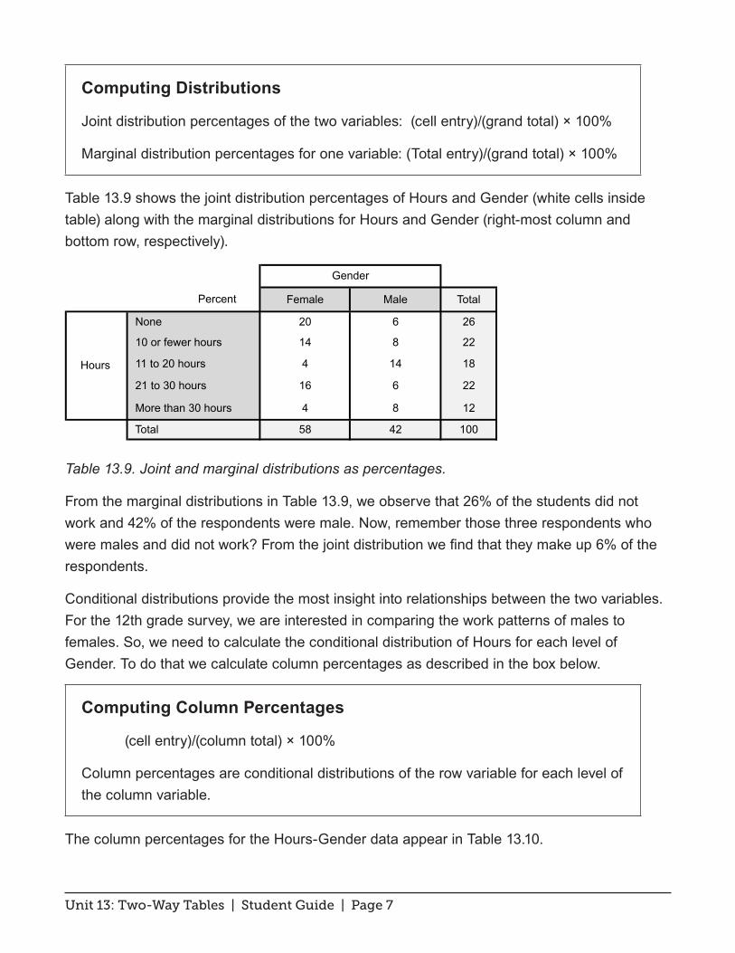
Computing Distributions
Joint distribution percentages of the two variables: (cell entry)/(grand total) × 100%
Marginal distribution percentages for one variable: (Total entry)/(grand total) × 100%
Table 13.9 shows the joint distribution percentages of Hours and Gender (white cells inside table) along with the marginal distributions for Hours and Gender (right-most column and bottom row, respectively).
Table 13.9. Joint and marginal distributions as percentages.
From the marginal distributions in Table 13.9, we observe that 26% of the students did not work and 42% of the respondents were male. Now, remember those three respondents who were males and did not work? From the joint distribution we find that they make up 6% of the respondents.
Conditional distributions provide the most insight into relationships between the two variables. For the 12th grade survey, we are interested in comparing the work patterns of males to females. So, we need to calculate the conditional distribution of Hours for each level of Gender. To do that we calculate column percentages as described in the box below.
Computing Column Percentages
(cell entry)/(column total) × 100%
Column percentages are conditional distributions of the row variable for each level of the column variable.
The column percentages for the Hours-Gender data appear in Table 13.10.
Female Male Total
None 20 6 26
10 or fewer hours 14 8 22
11 to 20 hours 4 14 18
21 to 30 hours 16 6 22
More than 30 hours 4 8 12
Total 58 42 100
Table 13.9
Percent
Gender
Hours

Unit 13: Two-Way Tables | Student Guide | Page 8
Table 13.10. Conditional distribution of Hours for each level of Gender.
Sometimes it is easier to take in information if it is presented graphically. The bar chart in Figure 13.2 is a graphical representation of the numbers in 13.10. The conditional distribution of Hours for females is represented by the first 5 bars on the left and the conditional distribution of Hours for males is represented by the last 5 bars on the right. One result that jumps out from looking at the bar chart is that the highest bar for females, associated with the response None (34.5%), is higher than the highest bar for males, associated with the response of working 11 to 20 hours per week (33.3%).
Figure 13.2. Bar chart of conditional distributions of Hours for each level of Gender.
Female Male
None 34.48 14.29
10 or fewer hours 24.14 19.05
11 to 20 hours 6.9 33.33
21 to 30 hours 27.59 14.29
More than 30 hours 6.9 19.05
Total 100 100
Table 13.10
Percent
Gender
Hours
Gender
Hours
Male
Female
More th
an 30
hours
21 to
30 ho
urs
11 to
20 ho
urs
10 or
fewer
hoursNo
ne
More th
an 30
hours
21 to
30 ho
urs
11 to
20 ho
urs
10 or
fewer
hoursNo
ne
40
35
30
25
20
15
10
5
0
19.0
14.3
33.3
19.0
14.3
6.9
27.6
6.9
24.1
34.5
Percent within levels of Gender.
Perc
ent

Unit 13: Two-Way Tables | Student Guide | Page 9
Similarly, we can compute the conditional distribution of Gender for each level of Hours. Since there are five values for the variable Hours, there will be five conditional distributions, one for each row of the table. We calculate these percentages as follows.
Computing Row Percentages
(cell entry)/(row total) × 100%
Row percentages are conditional distributions of the column variable for each level of the row variable.
The results appear in Table 13.11.
Table 13.11. Conditional distribution of Gender for each level of Hours
From Table 13.11, we learn that nearly 77% of the student respondents who did not work were female and that nearly 67% of the students who worked more than 30 hours per week were male.
Female Male Total
None 76.92 23.08 100%
10 or fewer hours 63.64 36.36 100%
11 to 20 hours 22.22 77.78 100%
21 to 30 hours 72.73 27.27 100%
More than 30 hours 33.33 66.67 100%
Table 13.11
Gender
Percent
Hours

Unit 13: Two-Way Tables | Student Guide | Page 10
Key Terms
Categorical variables can be either nominal, values that have no inherent order, or ordinal, values that have an inherent order. The inherent order of the values of an ordinal categorical variable should be preserved in tables and charts involving that variable.
A two-way table of counts (or frequencies) organizes data about two categorical variables taken from the same individuals or subjects. Values of the row variable label the rows of the table; values of the column variable label the columns of the table. A two-way table in which the row variable has n values and the column variable has m values is called an n × m table.
The sum of the row entries or the sum of the column entries are called the marginal totals. Marginal distributions are computed by dividing the row or column totals by the overall total. Marginal distributions provide information about the individual variables but do not provide any information about the relationship between the two variables.
A two-way table of counts can be converted into a joint distribution by dividing each cell count by the grand total and multiplying by 100%.
There are two sets of conditional distributions for a two-way table:
• distributions of the row variable for each fixed level of the column variable • distributions of the column variable for each fixed level of the row variable
Conditional distributions provide one way to explore the relationship between the row and column variables.
Unit 13: Two-Way Tables | Student Guide | Page 11
The Video
Take out a piece of paper and be ready to write down answers to these questions as you watch the video.
1. Give two (or more) examples of categorical variables.
2. What did Somerville include in its 2011 census that was unconventional?
3. In the two-way table used to organize the responses to rating personal happiness and Somerville’s physical beauty, which variable was the row variable and which was the column variable? Explain.
4. As the level of happiness went up (from Unhappy to So-so to Happy), what happened to the percent of respondents who rated Somerville’s physical beauty as Bad?
Unit 13: Two-Way Tables | Student Guide | Page 12
Unit Activity: Happiness Survey
Complete the survey at the end of this activity (or a modified version that your instructor provides). After you have responded to the survey, your instructor will distribute the class data. Answer the following questions based on the class data.
1. Organize the data on rating physical beauty and happiness into a two-way table. Use Happiness for the row variable and Beauty for the column variable. Add the marginal totals to your table.
In the rest of this activity, round percentages to one decimal.
2. What percentage of your class responded Happy? Show the appropriate calculation.
3. What percentage of your class rated the Physical Beauty of your campus or school as Good? Show the appropriate calculation.
4. a. Create a table showing the conditional distribution of Physical Beauty for each level of Happiness.
b. Were Happy students or Unhappy students more likely to respond that the Physical Beauty of campus was good? Support your answer with appropriate percentages. Show how these percentages were calculated.
5. a. Make a bar chart that represents the conditional distributions of Happiness for each level of Physical Beauty. Use a percent scale for the vertical axis and label each bar with its corresponding percent.
b. Write a few sentences describing what can be learned from your bar chart in (a).
6. Write a brief report analyzing the data from the remaining survey question(s). Include analysis of relationships between responses to the remaining survey question(s) and the survey questions involving Physical Beauty and Happiness. Include two-way tables and at least one graphic display in the report.

Unit 13: Two-Way Tables | Student Guide | Page 13
Happiness Survey
Circle your answers to the following questions:
What is your class year?
Fr So Jr Sr
Rate the physical beauty of your campus (or school):
Bad OK Good
Rate your level of happiness today:
Unhappy So-so Happy

Unit 13: Two-Way Tables | Student Guide | Page 14
Exercises
Each year the study Monitoring the Future: A Continuing Study of American Youth surveys students on a wide range of topics related to behaviors, attitudes, and values. These exercises are based on data collected from the 2011 survey of 12th grade students.
Table 13.12 organizes data on gender and responses to the following question:
How intelligent do you think you are compared with others your age?
Responses to this question have been boiled down into three categories: Below Average, Average, and Above Average.
Table 13.12. Results from questions on gender and intelligence.
Refer to Table 13.12 for questions 1 and 2.
1. a. Copy Table 13.12. Add a row to the bottom and a column to the right-end of your table. Compute the marginal totals and enter them into your table.
b. What percentage of the students who answered both questions were male? Female? Show your calculations. (Round percentages to one decimal.)
c. What percentage of the students rated their intelligence as above average? What does this tell you about 12th grade students’ assessment of their intelligence?
2. a. Compute conditional distributions of Intelligence for males and females. Record your results in a table. Show calculations. (Round percentages to one decimal.)
b. Represent the distributions in your table from (a) in a bar chart.
c. Write a brief description of how the male respondents rated their intelligence compared to female respondents.
Below Average Average Above
Average
Female 437 2243 4072
Male 456 1643 4593
Table 13.12
Intelligence
Gender

Unit 13: Two-Way Tables | Student Guide | Page 15
Table 13.13 organizes data on gender and responses to the following question:
How would you describe your political preference?
Responses to this question have been categorized as Rep (Republican), Ind (Independent), Dem (Democrat), Oth (Other), and No Pref/Hvnt Decid (No preference or haven’t decided).
Table 13.13. Results from questions on gender and political preference.
Questions 3 and 4 refer to Table 13.13.
3. a. Create a table showing the joint distribution (percentage) of gender and political preference. Add a row to the bottom and a column to the right end of your table. Enter the marginal distributions for gender and political preference into the added row and column. (Round percentages to one decimal.)
b. Create a table showing the conditional percentages for Political Preference for each gender. (Round percentages to one decimal.)
c. Create a table showing the conditional percentages of Gender for each category of Political Preference. (Round percentages to one decimal.)
4. Use the tables you created in question 3 to answer (a) – (d).
a. What percent of the respondents were females and Democrats? What percent of the respondents were males who were Independents?
b. Were male students or female students more likely to respond they were Republicans? Include relevant percentages in your answer.
c. Were Republicans more likely to be male or female? Be sure to include relevant percentages in your answer. Explain how this question differs from (b).
d. Make a graphic display that represents the distribution of Political Preference for each gender. Compare the political preferences of the 12th grade male students to the 12th grade female students.
No Pref/Hvnt Decid
Female 1275 723 1633 89 2917
Male 1620 871 1332 183 2577
Table 13.13
Gender
Political Preference
Rep Ind Dem Oth
Unit 13: Two-Way Tables | Student Guide | Page 16
Review Questions
The Monitoring the Future Study is a major source of information on smoking, drinking and drug habits of American youth. Based on data collected from the 2011 survey, you will decide whether or not smoking is linked to gender or if there is a linkage between high school grades and alcohol consumption. The review questions will focus on data collected from the following three survey questions:
I. On how many occasions (if any) have you had alcoholic beverages to drink – more than just a few sips during the last 30 days?
II. Have you ever smoked cigarettes?
III. Which of the following best describes your average grade so far in high school?
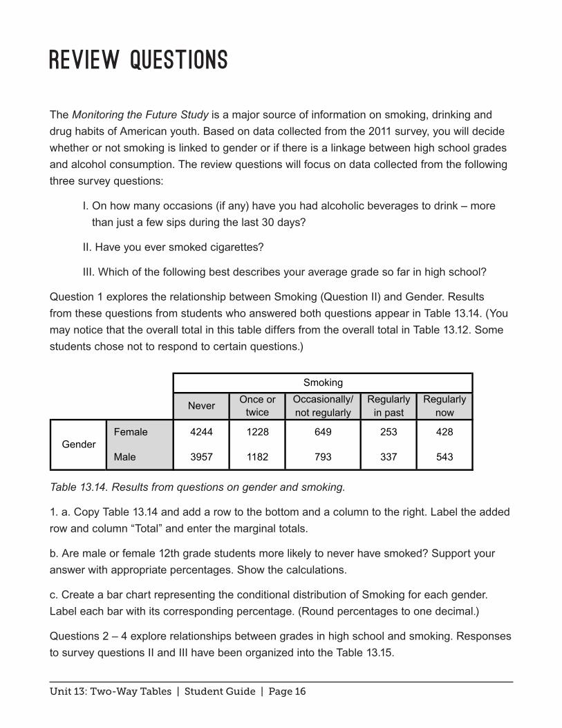
Question 1 explores the relationship between Smoking (Question II) and Gender. Results from these questions from students who answered both questions appear in Table 13.14. (You may notice that the overall total in this table differs from the overall total in Table 13.12. Some students chose not to respond to certain questions.)
Table 13.14. Results from questions on gender and smoking.
1. a. Copy Table 13.14 and add a row to the bottom and a column to the right. Label the added row and column “Total” and enter the marginal totals.
b. Are male or female 12th grade students more likely to never have smoked? Support your answer with appropriate percentages. Show the calculations.
c. Create a bar chart representing the conditional distribution of Smoking for each gender. Label each bar with its corresponding percentage. (Round percentages to one decimal.)
Questions 2 – 4 explore relationships between grades in high school and smoking. Responses to survey questions II and III have been organized into the Table 13.15.
Occasionally/ Regularly Regularlynot regularly in past now
Female 4244 1228 649 253 428
Male 3957 1182 793 337 543
Table 13.14
Smoking
Never Once or twice
Gender

Unit 13: Two-Way Tables | Student Guide | Page 17
Table 13.15. Responses to questions on grades and smoking.
2. a. How many students answered both the question on grades and the question on smoking?
b. What percentage of students answering both questions had never smoked? Had smoked at least once?
c. What percentage of students had average grades of A- or A and never smoked? Show the calculations. (Round answer to one decimal.)
3. a. What percentage of A- or A students have never smoked? Show the calculations.
b. What percentage of students’ whose averages are C+ or below never smoked? Show the calculations.
4. Next, you will examine the relationship between Smoking status and having a B- average or better.
a. What percentage of students who are regular smokers had averages B- or better?
b. What percentage of students who were regular smokers in the past had averages B- or better?
c. What percentage of students who never smoked had averages B- or better?
5. The graphic display in Figure 13.3 represents the conditional distribution of alcohol usage for each level of Grade. The conditional percentages (rounded to the nearest percent) appear above each bar.
Occasionally/ Regularly not regularly in past
D 46 22 23 12 25
C-, C, or C+ 926 436 323 123 285
B-, B, or B+ 3792 1275 769 330 489
A- or A 3465 665 327 126 168
Table 13.15
Grades
Smoking
Never Once or twice
Regularly now

Unit 13: Two-Way Tables | Student Guide | Page 18
Figure 13.3. Conditional distributions of Alcohol for each level of GPA.
a. Do the conditional percentages for each level of Grades sum to 100%? If not, explain why they might not sum to 100%.
b. Write a brief description of alcohol usage among the different levels of Grades. What relationship, if any, can you find between alcohol usage and grades?
HS Ave Grade
Alcohol Last 30 Days
A- or A
B-, B, o
r B+
C-, C, o
r C+D
6+ tim
es3-5
X1-2
X
0 Occa
s
6+ tim
es3-5
X1-2
X
0 Occ
as
6+ tim
es3-5
X1-2
X
0 Occ
as
6+ times
3-5X
1-2X
0 Occ
as
80
70
60
50
40
30
20
10
0
Perc
ent
68
18
67
1111
21
57
1513
21
51
1713
19
50
Percent within levels of HS Ave Grade.
Unit 14: The Question of Causation | Student Guide | Page 1
Unit 14: The Question of Causation
Summary of Video
Causation in statistics can be a tricky thing because appearances can often be deceiving. Observing an association between two variables does not automatically mean that there is a cause and effect relationship. One of the biggest challenges in attempting to prove causation comes from hidden factors. They might not be immediately apparent; they just lurk in the background. And that is exactly what we call them, lurking variables. For example, one study found that people who owned two or more cars tended to live longer than people who owned only one car. In this case, the lurking variable is the car buyer’s affluence. Richer individuals own more cars and tend to live longer, probably because they have better access to medical care and healthier food. The cars have nothing to do with it.
There are times, however, when causation seems to be the only reasonable explanation for the relationship between an explanatory variable and a response variable. A good example of this is the case of smoking and lung cancer. There was a time when smokers did not give a second thought to the health risks they might be taking. This is a far cry from today when anyone can tell you smoking causes lung cancer; it is even printed on cigarette packs. But how can we say for sure that smoking causes lung cancer? The fact that there is a strong association between smoking and lung cancer isn’t enough to show that smoking actually causes lung cancer. How do we know that the actual cause isn’t due to a lurking variable instead?
The best way to make a case for causation is to do an experiment. We could go to a local hospital and randomly assign newborn babies to one of two groups: those we force to smoke, and those we prevent from smoking. We keep the newborns in isolation to keep out lurking variables. As the newborns get older, we compare the cancer rates in each group. The only difference between the two groups would be their smoking habits. However, we can’t actually conduct such an experiment. So how can we get evidence for causation? The answer to this question was long in coming, but offers a fascinating look at biostatistical research.
Cigarette smoking became increasingly popular in America after World War I, when cigarettes were handed out to soldiers to boost morale. As smoking’s prevalence increased, so did lung cancer rates. A handful of doctors began to raise early warnings about the dangers

Unit 14: The Question of Causation | Student Guide | Page 2
of smoking. However, many doctors were smokers themselves and they didn’t believe that smoking was the culprit. But in the early 1940s, new studies sounded a louder alarm on the dangers of smoking. One of the earliest and most compelling was a retrospective study conducted by Ernst Wynder and Evarts Graham. This study compared people with and without lung cancer, looking for big differences in background or habits. Smoking stood out. They discovered that patients that had cancer of the lung were 17 times to 1 as apt to be two-pack-a-day smokers than non-cancer patients. Despite the remarkable discrepancy in smoking habits between the two groups of patients, this retrospective study was not good enough. Because the study looked at past behavior, behavior it could not control, it is possible that lung cancer was due to any number of lurking variables – such as DNA (a common cause), or polluted environments (a confounding factor), or even just coincidence.
The next step in solving this epidemiological mystery was setting up prospective studies. Doctors Hammond and Horn of the American Cancer Society gave about 200,000 people a smoking questionnaire and followed them for four years. Unlike a retrospective study, which begins with sick people – cancer patients – and works backwards to examine their habits, a prospective study looks ahead, following healthy people – both smokers and nonsmokers – forward through time to see which ones develop lung cancer. The results of this study caused quite a sensation. It showed that people who smoked cigarettes had a lung cancer rate 10 times higher than people who never smoked. However, there was still concern that lurking variables could be present, making the association between smoking and lung cancer only appear strong.
The association between smoking and lung cancer stood up in many different studies in different places and with different kinds of people. However, these were still not experiments. Researchers turned next to animal experiments, and they showed that cigarette smoke does contain substances that cause cancer in animals. These experiments also confirmed a dose/response relationship: more smoke causes more cancer.
Between 1940 and 1960, while this research was going on, per person cigarette consumption doubled. In 1962, the Surgeon General assembled a group of experts to review the entire issue. They concluded that there was excellent evidence that cigarette smoking did in fact cause lung cancer. Since the Surgeon General’s report, smoking has been under attack and has declined considerably.
The causal link between smoking and lung cancer was difficult to prove because direct experiments aren’t possible. In this case, the non-experimental evidence is about as strong as it gets – the link was established in many studies with different groups of people, the association was very strong, smoke did contain cancer-causing substances, and finally, no other explanation other than causation was plausible.

Unit 14: The Question of Causation | Student Guide | Page 3
Student Learning Objectives
A. Understand that an observed association between two variables need not be due to a cause-and-effect relationship between the two variables.
B. In simple situations, identify lurking variables that can affect the interpretation of an observed association between two other variables.
C. Recognize the distinction between an experiment, a prospective study, and a retrospective study.
D. Understand that good experiments give the best evidence for causation, and that in the absence of experiments, we must rely on a combination of other evidence.

Unit 14: The Question of Causation | Student Guide | Page 4
Content Overview
In Unit 10, Scatterplots, a scatterplot of manatee deaths and the number of powerboat registrations shows a positive association between the two variables. However, the fact that there is a relationship between two variables is not sufficient evidence to prove cause-and-effect linkage. A well-designed experiment in which the researcher imposes some treatment on its subjects to see how they respond can give good evidence for cause and effect as you will learn in Unit 15, Designing Experiments. The main thrust of this unit, however, is to look at the problem of assembling evidence for causation when experiments cannot be done.
Many investigations of major public issues seek to find cause-and-effect relationships without conducting experiments. Does living near high-tension lines, or having low concentrations of natural radon in your basement, or eating foods with preservatives, increase cancer risk? Does the prevalence of violent video games increase violence in society? Do lower speed limits reduce traffic deaths? Smoking and health is one example in which the question has been settled, but only after decades of study.
A strong observed association can be due to direct cause-and-effect. But it can also be due to the effects of another variable, which we call a lurking variable because it lurks in the background. For example, an article in a women’s magazine reported that women who nurse their babies feel more receptive toward their infants than mothers who bottle-feed. The author concluded that breast-feeding leads to a more positive attitude toward the child. But women choose whether to nurse or bottle feed, and this choice may reflect already existing attitudes toward their infants. Mothers who already feel more positive about the child may choose to nurse, for example, while those to whom the baby is a nuisance may be more likely to choose the bottle. The mothers’ already established attitude is a lurking variable that prevents conclusions about whether breast-feeding itself changes mothers’ attitudes.
To establish causation when an experiment cannot be done, we must amass a variety of less direct evidence. Retrospective and prospective studies can be part of that evidence. A retrospective study starts with an outcome (for example, a group of cancer patients and non-cancer patients) and then looks back to examine exposures to suspected risk factors or protective factors that might be linked to that outcome. A prospective study starts with a group (for example, a group containing smokers and nonsmokers) and watches for outcomes (cancer/no cancer) during the study period and relates this to suspected risk factors or protective factors that might be linked to the outcomes. Problems associated with lurking variables and bias are more common in retrospective studies than in prospective studies, so

Unit 14: The Question of Causation | Student Guide | Page 5
prospective studies would be preferred over retrospective studies. However, retrospective studies are faster to complete since researchers look back at data that have already been collected. Prospective studies require researchers to collect the data as the study progresses. In addition, retrospective studies are generally preferred if the outcome of interest is uncommon. In that case, the size of the group under study in a prospective study may need to be so large that it would be too costly to conduct the study.
Now, we return to the study on the question of smoking causing lung cancer that was featured in the video. For that study, the “good evidence” includes:
• The observed association is very strong (heavy smokers are about 20 times more likely to get lung cancer than nonsmokers).
• The association appears in many studies, both retrospective and prospective, of different groups in different places. Prospective studies are more convincing than retrospective studies.
• The effect regularly follows the alleged cause in time.
• There is a plausible causal mechanism (cigarette smoke contains substances that can be shown by experiments to cause cancer in animals).
• There is no similarly plausible explanation based on lurking variables (for example, heredity can’t account for the effect).
So, without an experiment where the levels of the explanatory variable are controlled and outcomes observed, it takes a great amount of evidence to establish a cause-and-effect relationship.

Unit 14: The Question of Causation | Student Guide | Page 6
Key Terms
A lurking variable is an extraneous variable that is related to other variables in a study. A lurking variable that is linked to both an explanatory variable and a response variable can be the underlying cause for an observed relationship between the explanatory and response variable.
A retrospective study starts with an outcome and then looks back to examine exposures to suspected risk or protective factors that might be linked to that outcome.
A prospective study starts with a group and watches for outcomes (for example, the development of cancer or remaining cancer-free) during the study period and relates this to suspected risk or protective factors that might be linked to the outcomes.

Unit 14: The Question of Causation | Student Guide | Page 7
The Video
Take out a piece of paper and be ready to write down answers to these questions as you watch the video.
1. People who own more cars tend to live longer than people who own fewer cars. Why is this relationship not evidence that buying more cars increases life expectancy?
2. Heavy smokers are about 20 times more likely to get lung cancer than nonsmokers. Why isn’t this link by itself good evidence that smoking causes lung cancer?
3. What is the difference between a retrospective study and a prospective study?
4. Why is a prospective study that compares a group of smokers with a similar group of nonsmokers not an experiment?
5. Why do experiments with animals add to the evidence that smoking causes cancer in humans?

Unit 14: The Question of Causation | Student Guide | Page 8
Unit Activity: Retrospective and Prospective Studies
Conduct an Internet search to find examples of each of the following. In each case, does the study prove a cause and effect relationship?
1. Find a retrospective study that starts with some outcome group and looks to see if it is associated with increased or decreased physical activity. Be prepared to share a summary of the study that you found with the class.
2. Find a prospective study that investigates whether some disease or disorder (you pick the disease or disorder) is related to a suspected risk or protective factor.
3. Find an example of either a retrospective study a or prospective study different from your examples in questions 1 and 2.
Unit 14: The Question of Causation | Student Guide | Page 9
Exercises
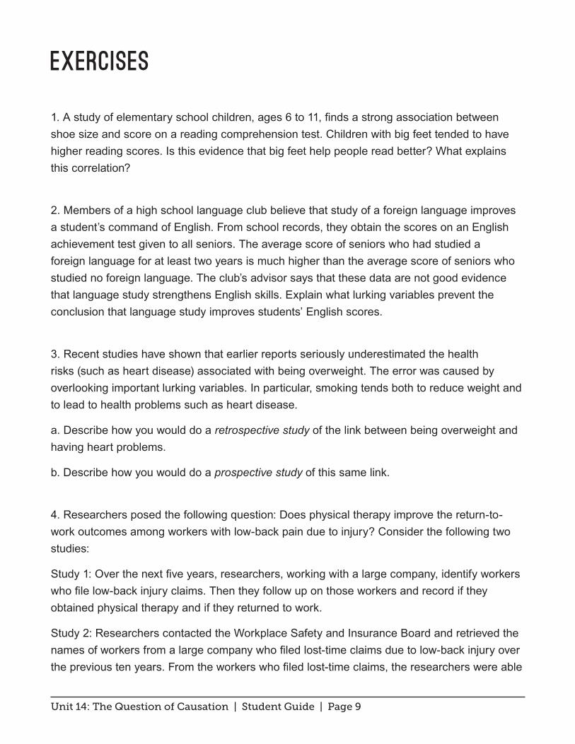
1. A study of elementary school children, ages 6 to 11, finds a strong association between shoe size and score on a reading comprehension test. Children with big feet tended to have higher reading scores. Is this evidence that big feet help people read better? What explains this correlation?
2. Members of a high school language club believe that study of a foreign language improves a student’s command of English. From school records, they obtain the scores on an English achievement test given to all seniors. The average score of seniors who had studied a foreign language for at least two years is much higher than the average score of seniors who studied no foreign language. The club’s advisor says that these data are not good evidence that language study strengthens English skills. Explain what lurking variables prevent the conclusion that language study improves students’ English scores.
3. Recent studies have shown that earlier reports seriously underestimated the health risks (such as heart disease) associated with being overweight. The error was caused by overlooking important lurking variables. In particular, smoking tends both to reduce weight and to lead to health problems such as heart disease.
a. Describe how you would do a retrospective study of the link between being overweight and having heart problems.
b. Describe how you would do a prospective study of this same link.
4. Researchers posed the following question: Does physical therapy improve the return-to-work outcomes among workers with low-back pain due to injury? Consider the following two studies:
Study 1: Over the next five years, researchers, working with a large company, identify workers who file low-back injury claims. Then they follow up on those workers and record if they obtained physical therapy and if they returned to work.
Study 2: Researchers contacted the Workplace Safety and Insurance Board and retrieved the names of workers from a large company who filed lost-time claims due to low-back injury over the previous ten years. From the workers who filed lost-time claims, the researchers were able

Unit 14: The Question of Causation | Student Guide | Page 10
to identify which of the workers requested reimbursement for physical therapy and which were able to return to work.
a. Which of the two studies is a retrospective study? Which is a prospective study? Justify your answer.
b. Which of the two studies is likely to be more costly? Explain.
c. Which of the two studies would be preferred in this situation? Why?

Unit 14: The Question of Causation | Student Guide | Page 11
Review Questions
1. A job-training program is being reviewed. Advocates claim that because the unemployment rate in the manufacturing region affected by the program was 9% when the program began and 5% four years later, the program was effective. Suggest lurking variables that might explain this outcome even if the program had no effect.
2. A study reported a positive association between using marijuana as a teen and having troubled relationships between ages 25 and 30. Based on this research should we conclude that teenagers’ use of marijuana leads to relationship problems during the latter half of their 20s? Explain.
3. Does regular exercise reduce the risk of a heart attack? A researcher finds 2000 men over 40 who exercise regularly and have not had heart attacks. She matches each with a similar man who does not exercise regularly, and she follows both groups for 10 years. Is this an experiment? What kind of study is it? Explain your answers.
4. Consider the following two studies:
Study 1: A group of 568 married white men aged 30 – 70 who died from coronary heart diseases and a matched sample of living white men with similar characteristics (matched age, socioeconomic level, body mass index (BMI), etc.) were part of a study to see if there was an association between increased leisure time devoted to physical activity and decreased coronary disease.
Study 2: A group of 32,269 women were enrolled in the Breast Cancer Detection Follow-Up Study. The goal of the study was to see if increased physical activity was associated with reduced breast cancer rates. Usual physical activity (including household, occupational, and leisure activities) was assessed from a self-administered questionnaire. Subsequent breast cancer cases were identified through self-reports, death certificates, and linkage to state cancer registries.
a. Would you classify Study 1 as a retrospective or prospective study? Justify your answer.
b. Would you classify Study 2 as a retrospective or prospective study? Justify your answer.
c. Why did Study 2 need so many participants in the study compared to Study 1?

Unit 15: Designing Experiments | Student Guide | Page 1
Unit 15: Designing Experiments
Summary of VideoStatistics helps us figure out the story hidden in a mound of data. Using statistics we can describe distributions, search for patterns, or tease out relationships. However, the reliability of our conclusions depends on the quality of the data collected.
One method of producing data is from an observational study. For the first story, we follow a team of marine scientists investigating how human populations affect coral reef ecosystems. They set up an observational study at four atolls in the remote Line Islands, each having a different history of human habitation. Kingman Reef has never had a human population; Palmyra was home to a military base during World War II but is no longer inhabited; Tabuaeran has a growing population of around 2,500; and Christmas Island has a population over 5,000. The research team recorded the size and quantity of predator fish, collected samples from each ecosystem, and took photographs of the coral. The scientists did not try to influence reef health – they simply observed it. They observed healthier ecosystems in areas with fewer humans. However, the problem with observational studies is they can’t prove anything about cause and effect. So, while the scientists observed less healthy ecosystems in areas with human population, they could not state that humans caused the damage to the coral reefs.
In order to establish causal relationships, researchers rely on experimental studies. An experiment imposes some treatment on its subjects to see how they respond. The second story focuses on a study of how certain dietary supplements affected the pain of osteoarthritis. Here researchers set up a double-blind randomized comparative experiment. Participants were randomly assigned to one of five treatment groups: Glucosamine, Chondroitin, combination of Glucosamine and Chondroitin, Celecoxib, and placebo. The latter two groups were control groups. The Celecoxib group received a standard prescription medication and the placebo group received a dummy pill. The response variable was the reported decrease in knee pain. When researchers calculated the mean reduction in pain after six months for each treatment group, it turned out that they all had fairly similar outcomes. So, the dietary supplements were no worse or better than the prescription medication, or even the placebo.
The osteoarthritis study was a well-designed experiment – researchers randomly assigned their subjects to treatments, the treatments included control groups, and the number of subjects was large. Next, we visit Dr. Confound as he collects data for his study on mood-altering medication. The video clip with Dr. Confound focuses on two hypothetical patients –

Unit 15: Designing Experiments | Student Guide | Page 2
his last two for his experiment, subjects 7 and 8. The patients get treated differently based on their initial mood – the one in a terrible mood is allowed to sit while the one in a good mood must stand. The doctor decides which medication to give each participant and he interacts with participants – adjusting one participant’s response and sympathizing with another’s. So this is a lesson in what not to do!

Unit 15: Designing Experiments | Student Guide | Page 3
Student Learning Objectives
A. Distinguish experiments from observational studies.
B. Recognize confounding in simple situations and the consequent weakness of uncontrolled studies.
C. Outline the design of a randomized comparative experiment to compare two or more treatments.
D. Understand how well-designed experiments can give good evidence for causation.
E. Use a table of random numbers or calculator/computer to generate random numbers in order to carry out a random assignment of subjects to treatment groups.
Unit 15: Designing Experiments | Student Guide | Page 4
Content Overview
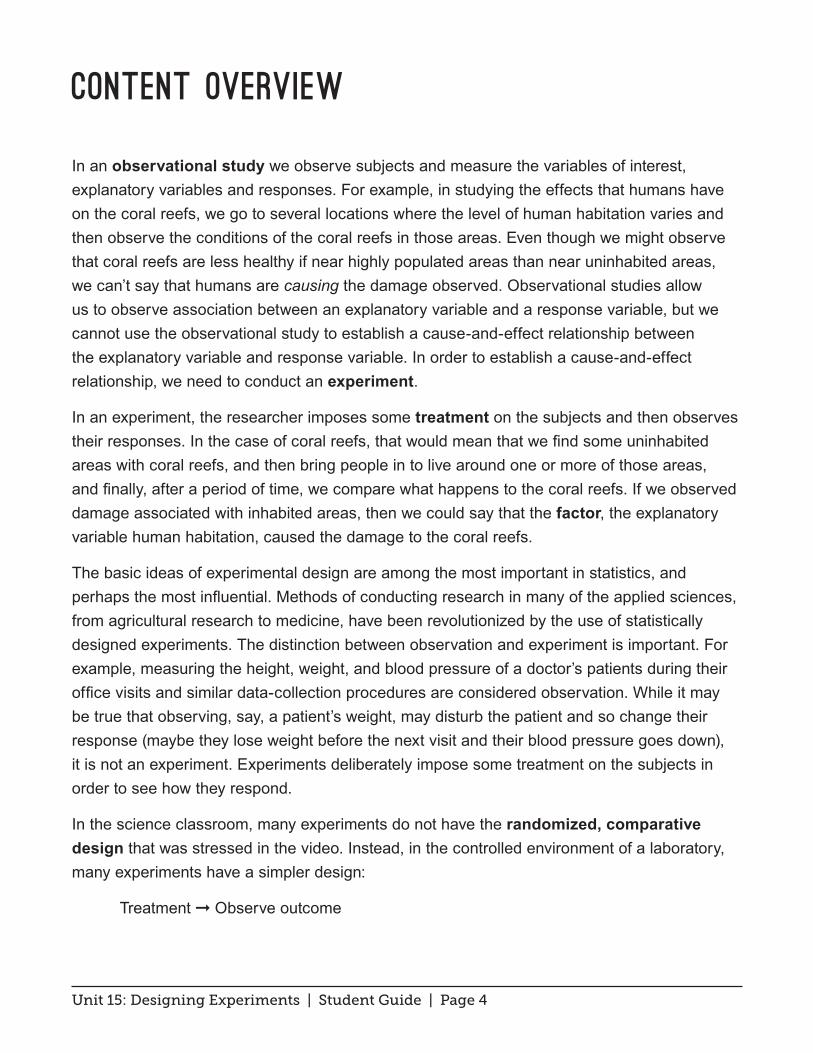
In an observational study we observe subjects and measure the variables of interest, explanatory variables and responses. For example, in studying the effects that humans have on the coral reefs, we go to several locations where the level of human habitation varies and then observe the conditions of the coral reefs in those areas. Even though we might observe that coral reefs are less healthy if near highly populated areas than near uninhabited areas, we can’t say that humans are causing the damage observed. Observational studies allow us to observe association between an explanatory variable and a response variable, but we cannot use the observational study to establish a cause-and-effect relationship between the explanatory variable and response variable. In order to establish a cause-and-effect relationship, we need to conduct an experiment.
In an experiment, the researcher imposes some treatment on the subjects and then observes their responses. In the case of coral reefs, that would mean that we find some uninhabited areas with coral reefs, and then bring people in to live around one or more of those areas, and finally, after a period of time, we compare what happens to the coral reefs. If we observed damage associated with inhabited areas, then we could say that the factor, the explanatory variable human habitation, caused the damage to the coral reefs.
The basic ideas of experimental design are among the most important in statistics, and perhaps the most influential. Methods of conducting research in many of the applied sciences, from agricultural research to medicine, have been revolutionized by the use of statistically designed experiments. The distinction between observation and experiment is important. For example, measuring the height, weight, and blood pressure of a doctor’s patients during their office visits and similar data-collection procedures are considered observation. While it may be true that observing, say, a patient’s weight, may disturb the patient and so change their response (maybe they lose weight before the next visit and their blood pressure goes down), it is not an experiment. Experiments deliberately impose some treatment on the subjects in order to see how they respond.
In the science classroom, many experiments do not have the randomized, comparative design that was stressed in the video. Instead, in the controlled environment of a laboratory, many experiments have a simpler design:
Treatment ➞ Observe outcome

Unit 15: Designing Experiments | Student Guide | Page 5
For example,
Mix chemicals ➞ Observe explosion
However, for agricultural or ecological experiments in the field or in experiments involving living subjects that vary a lot, this simple design invites confounding – mixing of a variety of causes, even those not considered in the experiment. Uncontrolled medical experiments, for example, have led doctors to conclude that worthless treatments worked. The natural optimism of the doctors who had invented the treatment, the placebo effect (the strong effect on patients of any treatment given even if the treatment is fake), and perhaps an unrepresentative group of patients combined to make the worthless treatments look good. Later, randomized comparative experiments found that the treatments had no value. Doctors gradually recognized that well-designed experiments were essential.
Agricultural researchers learned this earlier. Variation in the weather alone is enough to force experiments with new crop varieties to be comparative. The yield of a new variety this year may look great, but this was a good growing season. The virtues of the new variety are confounded with the effects of weather unless we do a comparative experiment in which older varieties were also grown. Unpredictable variation in soil makes random assignment of competing crop varieties to small growing plots desirable. In fact, statistical design of experiments first arose in the 1920s to solve the problems encountered by agricultural field trials.
Principles of experimental design
The basic principles of statistical design of experiments are:
1. Randomization: Use of impersonal chance to assign subjects to treatments to remove bias and other sources of extraneous variation. Randomization produces groups of subjects that should be similar in all respects before the treatments are applied. It allows us to equalize across all treatments the effects from unknown or uncontrollable sources of variation.
2. Replication: Repeat the experiment on many subjects to reduce chance variation in the results.
3. Local Control: Control all factors except the ones under investigation. Some examples of local control include: assigning equal numbers of subjects to each treatment, applying treatments uniformly and under standardized conditions, sorting subjects into homogeneous groups, and comparing two or more treatments.

Unit 15: Designing Experiments | Student Guide | Page 6
In a randomized comparative design subjects are randomly assigned to treatment groups in order to study the effect the treatment has on the response. Figure 15.1 is an outline of the basic design for comparing two treatments.
Figure 15.1. Outline of basic design for comparing two treatments.
Use this pictorial description rather than attempting a full description in words of an experimental design. Make the general design specific by adding the size of the groups, substituting the actual treatments compared (in place of Treatment #) and the response recorded. Notice that “treatment” is used for whatever is imposed on the subjects in an experiment, not only medical treatments.
The logic behind a randomized comparative design is straightforward. Randomization produces groups of subjects that should be similar in all respects before the treatments are applied. A comparative design ensures that influences other than the experimental treatments operate equally on all groups. Therefore, differences in the response variable must be due to the effects of the treatments – that is, the treatments are not only associated with the observed differences in the response, but must actually cause them.
To do the random assignment of subjects to groups, use a table of random digits or a random number generator (which is built into graphing calculators, as well as into spreadsheet and statistical software).
Randomizing treatments using a table of random digits
You can find a table of random digits in most introductory statistics textbooks as well as on the Internet. A random digits table has the following properties:
• Each entry in the table is equally likely to be any of the 10 digits 0, 1, 2, 3, 4, 5, 6, 7, 8, 9.
• The entries are independent of each other. That is, knowledge of one part of the table gives no information about any other part.
Group 1
Group 2
Treatment 1
Treatment 2
CompareResponse
RandomAllocation

Unit 15: Designing Experiments | Student Guide | Page 7
A random digits table is one long string of random digits. The numbers are generally arranged in groups of five and the rows numbered for convenience. Two digits from the table are equally likely to be any of the 100 possibilities 00 to 99, and so on. To choose at random, assign the subjects numerical labels and let the table choose from these labels at random.
For example, to choose at random 10 out of 20 subjects to get Treatment 1 (aspirin), label the subjects 01 to 20 and enter the random digits table on any line (vary the entry point each time you use the table), say line 110, which is given below.
38448 48789 18338 24697 39364 42006 76688 08708
Read two-digit groups because we assigned two-digit labels. Just skip over all groups not used as labels. So, skip 38, 44, 84, 87, and 89. The first subject chosen has label number 18. Continue this process until 10 subjects are chosen – next select 20, 06, 08, and so forth. Assign the 10 selected subjects to the aspirin treatment. The remaining subjects get the placebo.
Randomizing treatments using a random number generator
Graphing calculators and spreadsheet and statistical computing software have random number generators. Rand (TI graphing calculators and Excel) generates a number from the uniform distribution on the interval from 0 to 1. Suppose you have a list of 10 subjects and you want to choose five of them to assign to Treatment 1 (aspirin).
Step 1: Use a random number generator to assign a random number to each person. Excel’s Rand() was used to generate the set of random numbers in Table 15.1.
Table 15.1. Assigning a random number to subjects.
Subjects Rand Joe 0.305127 Sally 0.130861 Kelly 0.335956 Bruce 0.525466 Marsha 0.288252 Caitlin 0.036762 George 0.084562 Jian 0.763097 Cheryl 0.753380 Ying 0.775420
Table 15.1

Unit 15: Designing Experiments | Student Guide | Page 8
Step 2. Sort the names so that the first name is the name associated with the smallest random number and the last name is associated with the largest random number. Table 15.2 shows the results.
Table 15.2. Names sorted by random number.
Step 3. Select the first five names from the sorted list to assign to the aspirin treatment.
So, in this case, Caitlin, George, Sally, Marsha, and Joe would be assigned to the aspirin treatment and the remaining subjects would be assigned to the placebo group.
Who knows who is getting which treatment?
Particularly in the context of medical studies, it is important to know whether or not the participants know which treatment they are getting and whether or not those recording the responses know. In double-blind experiments neither the participants nor those conducting the experiment know which participants were assigned to which treatments. In a single-blind experiment the participants do not know which treatment they are receiving but those conducting the experiment do know.
Subjects Rand Caitlin 0.036762 George 0.084562 Sally 0.130861 Marsha 0.288252 Joe 0.305127 Kelly 0.335956 Bruce 0.525466 Cheryl 0.753380 Jian 0.763097 Ying 0.775420
Table 15.2

Unit 15: Designing Experiments | Student Guide | Page 9
Key Terms
In an observational study researchers observe subjects and measure variables of interest. However, the researchers do not try to influence the responses. The purpose is to describe groups of subjects under different situations. In an experimental study, researchers deliberately apply some treatment to the subjects in order to observe their responses. The purpose is to study whether the treatment causes a change in the response.
In a double-blind experiment neither the subjects nor the individuals measuring the response know which subjects are assigned to which treatment. In a single-blind experiment the subjects do not know which treatment they are receiving but the individuals measuring the response do know which subjects were assigned to which treatments.
A placebo is something that is identical in appearance to the treatment received by the treatment group but has no effect.
A control group is an experimental group that does not receive the treatment under study. The control group could receive a placebo to hide the fact that no treatment is being given. In an active control group, the subjects receive what might be considered the existing standard treatment.
The explanatory variables in either an observational study or experiment are called factors. A treatment is any specific condition applied to the subjects in an experiment. If an experiment has more than one factor, then a treatment is a combination of specific values for each factor.
Two factors (explanatory variables) are confounded when their effects on a response variable are intertwined and cannot be distinguished from each other.
Unit 15: Designing Experiments | Student Guide | Page 10
The Video
Take out a piece of paper and be ready to write down answers to these questions as you watch the video.
1. Why is the study of the effect of humans on the coral reefs not an experiment?
2. Who were the subjects in the Glucosamine/Chondroitin study? What did researchers want to find out?
3. Why were subjects randomly assigned to the treatments?
4. Dr. Confound conducted a very badly designed experiment on mood-altering medication. List some of the problems with his experiment.

Unit 15: Designing Experiments | Student Guide | Page 11
Unit Activity: In the News
Find an article in the print news (newspaper, online news, magazine) that reports on the results of a medical experiment. Describe what information appears in the article about the design of the experiment. Be prepared to discuss your news item in class.

Unit 15: Designing Experiments | Student Guide | Page 12
Exercises
1. It has been suggested that women and men differ in their political preferences. Women may be more likely than men to prefer Democratic candidates. A political scientist selects a large sample of registered voters, both men and women, and asks them whether they voted for the Democratic or Republican candidate in the last Congressional election. Is this study an experiment? Why or why not?
2. Before a new variety of frozen muffins is put on the market, it is subjected to extensive taste testing. People are asked to taste the new muffin and a competing brand, and to say which they prefer. (The muffins are not identified in the test.) Is this an experiment? Why or why not?
3. You are testing a new medication for relief of migraine headache pain. You intend to give the drug to migraine sufferers and ask them one hour later to estimate what percent of their pain has been relieved. You have 40 patients available to serve as subjects.
a. Outline an appropriate design for the experiment, taking the placebo effect into account.
b. The names of the subjects are given in Table 15.3. Either use a random digits table beginning at line 131 to do the randomization required by your design or use a calculator’s or computer software’s random number generator. List the subjects to whom you will give the drug. Explain how you arrived at this assignment.
Table 15.3. Names of subjects.
4. Determine which of the experiments below are single-blind, double-blind, or neither. Justify your answer.
Abrams Daniels Halsey Lippman Rosen Adamson Durr Howard Martinez Solomon Afifi Edwards Hwang McNeill Thompson Brown Fluharty Iselin Morse Travers Cansico Garcia Janle Ng Turner Chen Gerson Kaplan Obramowitz Ullman Cranston Green Krushchev Rivera Williams Curzakis Gutierrez Lattimore Roberts Wong
Table 15.3

Unit 15: Designing Experiments | Student Guide | Page 13
a. Dr. Colman has a home remedy that he thinks will help his patients recover from colds. He arranges for a colleague to have two sets of identical looking pills made up and bottled – pill A contains his remedy and pill B is a placebo. He recruits some of his patients to take part in the experiment. They are told that they will be randomly assigned to his remedy or a placebo. Dr. Colman does not know which bottles of pills, A or B, contain his remedy. After six months, Dr. Colman interviews his patients to check on the number of colds they contracted and the duration. He then summarizes his results in a report before learning from his colleague which group of participants got his remedy.
b. Pam decides that she wants to know what type of diet cola tastes best – Diet Coke, Caffeine Free Diet Coke, or Coca Cola Zero. So she invites a group of friends over for a taste test. She sets an unopened bottle of each type of soda on a table with some paper cups. Each of the participants pours some cola from each bottle into paper cups, marking the cups with the type of soda. Then they taste each type of diet soda and give Pam their rating – 1 (tastes awful) to 5 (tastes great).
c. Janet wants to know whether her secret recipe for chocolate cake will taste better if she uses cocoa or baking chocolate. She bakes two cakes that appear identical and asks a group of her friends to take part in a taste test. She labels the cake with cocoa as A and the cake with baking chocolate as B. Then she randomly assigns half her friends to taste cake A and the other half to taste cake B. Her friends are then asked to rate each cake from 1 to 10.
Unit 15: Designing Experiments | Student Guide | Page 14
Review Questions
1. You wish to learn if students in an English course write better essays when they are required to use computer word-processing than when they write and revise their essays by hand. There are 120 students in an English course available as subjects.
a. Outline the design of an experiment to determine if word-processing results in better essays.
b. What precautions would you take in doing this experiment that don’t appear in your outline of the design?
2. Two second grade teachers, Miss Earls (who has been teaching for 10 years) and Mrs. Morrow (who has been teaching for two years), were really excited by a new curriculum that used animations to teach science. They decided to use their classrooms for an experiment. Since Miss Earls had access to computers in her class, she used the animation lessons. Mrs. Morrow covered similar material with her students using handouts followed by discussions. After students had completed the materials, they were given a test designed by Miss Earls. There were 21 students in Miss Earls’ class and 29 students in Mrs. Morrow’s class. Miss Earls’ class scored, on average, 15 points higher on the test. The two teachers decided that the animation science series was an excellent series. Based on this study, Miss Earls talked her school into purchasing this curriculum.
Critique the study conducted by Miss Earls and Mrs. Morrow. Do you think Miss Earls’ school made a good decision in purchasing the animation science curriculum based on this study?
3. A study reported in the Annals of Internal Medicine (January 2010) followed 10,892 middle-aged adults over a nine year period. At the start of the study none of the subjects had diabetes. Roughly 45% of the subjects were smokers. The study found that compared to those who never smoked, subjects who quit smoking had an increased risk of diabetes.
a. Is the study described above an observational study or an experiment? Explain.
b. Based on this study, should you conclude that quitting smoking causes diabetes? Justify your answer.
4. The research question for an undergraduate research project was whether hearing-impaired consumers were treated differently by store clerks than non-hearing-impaired consumers.

Unit 15: Designing Experiments | Student Guide | Page 15
There were 20 consumers, 10 of whom were hearing impaired. The consumers were sent in pairs into stores. The hearing-impaired pairs used sign language to communicate with each other and the non-hearing impaired pairs entered stores speaking English to each other. The subjects consisted of 77 sales clerks in 27 stores (from the 175 stores) in a large shopping mall. The response variable was the time from when the pair entered the store and made eye contact with the sales clerk until the clerk approached and offered assistance.
Describe how you would design the rest of the experiment.

Unit 16: Census and Sampling | Student Guide | Page 1
Unit 16: Census and Sampling
Summary of VideoThere are some questions for which an experiment can’t help us find the answer. For example, suppose we wanted to know what percentage of Americans smoke cigarettes, or what per-centage of supermarket chicken is contaminated with salmonella bacteria. There is no experi-ment that can be done to answer these types of questions. We could test every chicken on the market, or ask every person if they smoke. This is a census, a count of each and every item in a population. It seems like a census would be a straightforward way to get the most accurate, thorough information. But taking an accurate census is more difficult than you might think.
The U.S. Constitution requires a census of the U.S population every ten years. In 2010, more than 308 million Americans were counted. However, the Census Bureau knows that some people are not included in this count. Undercounting certain segments of the population is a problem that can affect the representation given to a certain region as well as the federal funds it receives. What is particularly problematic is that not all groups are undercounted at the same rate. For example, the 2010 census had a hard time trying to reach renters.
The first step in the U.S. Census is mailing a questionnaire to every household in the country. In 2010 about three quarters of the questionnaires were returned before the deadline. A census taker visits those households that do not respond by mail, but still not everyone is reached. Some experts favor adjusting the census to correct the undercount using information gathered by smaller but more intense samples.
There is an alternative to a census, and that is a sample. While a census is an attempt to gather information about every member of the population, sampling gathers information only about a part, the sample, to represent the whole. Because a sample is only part of the popula-tion, we can study it more extensively than we can all of the members of the population. Then we can use the sample data to draw conclusions about the entire population. However, for those conclusions to be valid, the sample must be representative of the population. To make sure that it is, statisticians often rely on what is called simple random sampling. That means the sample is chosen in such a way that each individual has an equal chance to be selected. This helps eliminate bias in the study design, which occurs if certain outcomes are systemati-cally favored.

Unit 16: Census and Sampling | Student Guide | Page 2
Sampling is widely used in a variety of areas such as industry, manufacturing, agriculture, and medical studies, to name just a few. For example, consider food manufacturing with a look at processes Frito-Lay uses in making potato chips. Here’s just some of what happens. A truck carrying 45,000 pounds of raw potatoes arrives at the plant, but is not allowed to unload until a sample of its potatoes has been carefully tested. First, a 150-pound sample of potatoes is taken from different locations in the truck (some from the front, middle and back). Next, an inspector selects 40 pounds of those potatoes and punches a hole through the core. Those holes make it easy to spot the samples when they undergo a cooking test. In other potatoes, the inspector searches for internal defects, green edges, rot, and other flaws. Each defective potato is weighed, and if the sample percentage is too large, the whole load must be rejected. The cooking sample is peeled and tossed directly into the slicing machine. Then the sample chips with their telltale holes are plucked out and go to a mini laboratory for further testing. Once everything in the sample is found to be up to specifications, Frito-Lay will accept the multi-ton shipment, based on the 150-pound sample.
All along the production line, workers continue taking samples to ensure the chip-making pro-cess stays on track. Sample chips are measured for thickness, color, and salt content. Even the finished bags are sampled to check their weight, both before and after being packed into cartons. If Frito-Lay waited until the end of the line to inspect the finished product, problems that were minor to begin with could be greatly compounded. Instead, sampling at key points catches problems early, before they get out of hand.

Unit 16: Census and Sampling | Student Guide | Page 3
Student Learning Objectives
A. Know that a census is an attempt to enumerate the entire population; understand that a census is needed for information about every small part of the population, but for information about the population as a whole, a sample is faster, cheaper, and at least as accurate (if not more accurate).
B. Recognize the distinction between population and sample.
C. Recognize the strong bias in voluntary response samples, and generally in samples that result from human choice.
D. Know what a simple random sample is and how to use a random digits table or computer random number generator to select a simple random sample.
Unit 16: Census and Sampling | Student Guide | Page 4
Content Overview
A census is an attempt to gather information about every member of some group, called the population. This unit introduces the U.S. Census and its problems in collecting data on the entire U.S. population. One of the most serious problems is undercounting certain segments of the population. Unfortunately not all groups of people are undercounted at the same rates. For example, undercount rates for minority groups are higher than for whites and undercounted rates for renters are higher than for homeowners. Moreover, undercount rates for those living in poverty are higher than for the affluent. The U.S. government uses sampling to estimate undercount rates for various groups. However, it never changes the official headcount number based on the results from sampling.
A sample allows the researcher to gather information from only a part of the population. Sam-pling – collecting data from a portion of the population – is the general means of gathering information about a population when it is not possible to get information from each individual in the population. Sampling saves both time and money. In some cases, such as for Frito-Lay potato chips, both the whole potatoes in a sample and the chips in a sample are destroyed as part of the data collection process. In such cases a census would be out of the question or there would be no product left to sell.
In order for a sample to provide good information about a population, the sample needs to be representative of the population. A simple random sample, a sample in which each member of the population is equally likely to wind up in the sample, is one means of ensuring that the sample is representative of the population and not biased. A simple random sample can be selected from the population in the same way that a subgroup is randomly selected from a larger group to receive a certain treatment. Hence, you should refer to Unit 15, Designing Experiments, for directions on selecting a random sample.
Sampling bias occurs when a sample is collected in such a way that some members of the population are less likely to be included than others. A voluntary television poll is an example of a biased sample. Since it is voluntary, only those with strong views are likely to call or text in to vote. Furthermore, only those watching the particular station at the time the poll is given will participate. In this case, the entire segment of the population who do not watch that particular station will be left out of the sample.

Unit 16: Census and Sampling | Student Guide | Page 5
Key Terms
The entire group of objects or individuals about which information is wanted is called the population.
A census is an attempt to gather information about every individual in a population.
A sample is a part of the population that is actually examined in order to represent the whole. A simple random sample of size n consists of n individuals from the population chosen in such a way that every set of n individuals has an equal chance of being the selected sample.
Sampling bias occurs when a sample is collected in such a way that some individuals in the population are less likely to be included in the sample than others. Because of this, information gathered from the sample will be slanted toward those who are more likely to be part of the sample.
Unit 16: Census and Sampling | Student Guide | Page 6
The Video
Take out a piece of paper and be ready to write down answers to these questions as you watch the video.
1. Are recent U.S. Censuses more or less accurate than early Censuses?
2. Why is the U.S. Census undercount, which is quite small as a percent of the population, so important?
3. What is a simple random sample?
4. How many uses of sampling can you spot in the account of Frito-Lay potato chips?

Unit 16: Census and Sampling | Student Guide | Page 7
Unit Activity: The U.S. Census
Use a search engine (such as Google) to find the 2010 (or most recent) Census homepage. Then answer the following questions.
1. What is the current U.S. population? (Note this number will change. Check back at the end of the assignment to see how much the population has changed during the time you worked on this assignment.)
2. Click the Population Finder. Select your state from the scroll-down menu to access the 2010 (or most recent) Demographic Profile for your state.
a. What was the population of your state in 2010?
b. What percentage of your state’s population was male? Female?
c. Which was higher for your state, the percent under 18 or the percent 65 or over? (Give the percentages.)
3. Select another state that is close to your state. Write a brief paragraph comparing the demo-graphics of the two states.

Unit 16: Census and Sampling | Student Guide | Page 8
Exercises
1. A local television station takes quick polls of public opinion by announcing a question on the 6 o’clock news and asking viewers to call-in or text their opinion of “Yes” or “No” to the station. The results are announced on the 11 o’clock news. One such poll finds that 73% of those who called in or texted are opposed to a proposed local gun control ordinance.
a. What do you think the population is in this situation?
b. Explain why this sampling method is biased. Is the percent of the population who oppose gun control probably higher or lower than the 73% of the sample who are opposed?
2. The students named below are enrolled in a new statistics course. Use a random digits table (such as Table B in The Basic Practice of Statistics) at line 136 or a calculator/computer random number generator to choose five of these students at random to be interviewed in detail about the quality of the course. Explain how you chose your sample.
Agarwal Dewald Hixson Puri Anderson Fernandez Klassen Rodriguez Baxter Frank Mihalko Rubin Bowman Fuhrmann Moser Santiago Bruvold Goel Naber Shen Casella Gupta Petrucelli Shyr Cordero Hicks Pliego Sundheim
3. On the Hudson Valley, NY Patch Facebook page, readers were asked to send in stories of awful Valentine’s Day gifts. The following were selected:
• Leftover chocolate (and he had eaten one!)• Flowers purchased the day BEFORE Valentine’s because it was cheaper to buy
them the day before• A recycled card from an ex-boyfriend with an open box of chocolates
Readers were then asked to vote on the best “worst Valentine’s Day gift ever” story.

Unit 16: Census and Sampling | Student Guide | Page 9
a. Describe the population.
b. Describe the sample.
c. Do you think the response to this poll is representative of the views of the residents of Hudson Valley, New York? Explain.
4. Identify the population and the sample in each of the following situations.
a. A realtor is interested in the median selling price of homes in Worcester County, Massachu-setts. She collects data on the selling prices of 50 homes.
b. A psychologist is concerned about the health of veterans who served in combat. She exam-ines 25 veterans to assess whether or not they are showing signs of post-traumatic stress disorder (PTSD).
c. An educator asks 20 seniors from Eastern Connecticut State University whether or not they had taken an online course while at the university.

Unit 16: Census and Sampling | Student Guide | Page 10
Review Questions
1. The students listed below are enrolled in an elementary French course. Students are assigned to small conversation sections at random.
a. Choose a simple random sample of eight of these students to form Section 01. Explain how you obtained the names for the first section.
b. Assign the remaining students at random to the Sections 02, 03, 04, 05 and 06. Explain the process you used to make the assignments.
2. Identify the population and the sample in each of the following situations.
a. A professor asks a sample of students during their college orientation whether they planned to take an online course their first semester at college.
b. A physical therapist is investigating a new exercise regimen to see if it could improve the function of arthritic knees. She chooses 10 of her patients and has them follow the new exercise regimen.
3. A university president wishes to know what types of activities and jobs graduates of the university are doing 5 years after graduation. You have been asked to deliver this information to the president.
Arnold Ashford Bartkowski Barrett Beerbohm Burns Campbell Chang Colon Deneuve Dodington Drummond Elsevier Erskine Garcia Fernandez Flury Hardy Holmes Hyde Jones Juarez Kempthorne Levine Martinez Moore Munroe Neale Nguyen Oakley Orsini Perlman Poe Prizzi Putnam Quincy Randall Rodriguez Rostenkowski Rowley Schiller Scott Smith Stevenson Swokowski Taylor Vuong Ward
Review Question 1a

Unit 16: Census and Sampling | Student Guide | Page 11
a. What is the population of interest?
b. State reasons for taking a sample rather than a census to obtain information for the president.
4. Suppose you want to know whether or not a population supports a certain measure. You have one month to find out.
a. List some of the pros and cons for getting this information by conducting a census.
b. List some of the pros and cons for getting information about a population by taking a sample.

Unit 17: Samples and Surveys | Student Guide | Page 1
Unit 17: Samples and Surveys
Summary of VideoListen to a news broadcast, read a newspaper, open a magazine and you’ll find an item related to the results of a poll on some topic. But how do pollsters survey a population as large and diverse as the United States and wind up with a complete and unbiased picture of attitudes on a particular topic? Before selecting the sample to be surveyed, pollsters need to identify the population – the group of interest to the study.
For example, that could be all registered voters, people in a particular age group, or households with a certain income. The characteristic of a population that we are interested in is called a parameter. We can’t determine the true value of a parameter unless we can examine the entire population, which isn’t usually possible. However, we can estimate the unknown parameter based on information collected from a sample, a subset of the population. Such an estimate is called a statistic. (Remember Parameters are for Populations and Statistics are for Samples.)
The pollsters at the University of New Hampshire’s Survey Center conduct everything from academic research to political polls. They are experts at selecting samples to represent the attitudes and opinions of the whole population. For a public opinion survey they use random digit dialing to select households; they start with a random sample of households. However, another sampling stage is required because they talk to an individual at each house and not to everyone in the house. So, for example, they might ask to speak to the person in the house who has had the most recent birthday.
Convenience sampling, where pollsters survey a convenient group such as their friends, or voluntary sampling, where data are collected from those who volunteer for the survey, often create an unrepresentative sample and produce biased results. The same issue arises when a sample draws from a list that excludes a portion of the population. This happened in the 1936 presidential election when a Literary Digest poll predicted Alf Landon would be the winner. However, Franklin Roosevelt went on to win in a landslide. The Literary Digest drew their samples from lists of car and telephone owners – items that, at the time, were indicative of wealth. The poll had omitted the largely pro-Roosevelt poor from their survey, causing bias in favor of Landon.

Unit 17: Samples and Surveys | Student Guide | Page 2
Getting a representative sample is the cornerstone of accurate sampling. But just as important as a representative sample is the design of the questionnaire. Some practical advice on questionnaires includes using simple words, not asking people about things they are not likely to know about, and keeping the questions short. Even small things such as changing the order in which you read the choice of responses to survey participants can change how they answer a question.
In a simple random sample, each individual of the population has an equal chance of being selected. This can be hard to achieve in a real-life survey since it can be nearly impossible to get a complete list that includes every single member of a large population. Another way of ensuring a representative sample is by doing a multistage sample. For example, the Survey Center might begin with a random sample of counties in New Hampshire. Then they would take a random sample of towns within those counties. Finally they would select random households within those towns.
The problem with multistage sampling is that it could leave out groups of interest merely by chance. To solve this problem, the Survey Center might decide to use a stratified random sample. For this type of sampling design, the entire population is divided into groups with similar characteristics called “strata.” For example, census tracts might first be classified as urban, rural, or suburban, and then a separate random sample is selected from each stratum. In New Hampshire this ensures that cities are represented in the sample even though most counties are rural.

Unit 17: Samples and Surveys | Student Guide | Page 3
Student Learning Objectives
A. Realize that most national social and economic data are produced by large-scale sample surveys.
B. Know that samples of large, geographically dispersed human populations rarely use a simple random sample; be familiar with multistage samples and stratified samples.
C. Recognize that non-statistical aspects of sampling such as training of interviewers and wording of questions can have strong effects on the results of a sample survey.

Unit 17: Samples and Surveys | Student Guide | Page 4
Content Overview
This unit describes methods related to conducting surveys. Particularly when populations are large, geographically-dispersed human populations, it would be nearly impossible to include everyone in a survey. So, one aspect of conducting a good survey is the sampling design – the method used to choose a sample that is representative of the population. Equally important are the design of the questions and interviewer training.
Convenience sampling and voluntary sampling are two methods for choosing a sample that may not produce a representative sample. In convenience sampling, a sample is chosen in a way that makes it easy to obtain. For example, the pollster could stand outside a grocery store on some weekday morning and interview people as they enter the store. That would be an easy way to get a sample, but the sample probably won’t be representative of the opinions of the population – for one thing, most likely there will be more women in the sample than men, and the sample won’t contain people who work weekdays 9 to 5. So the sample will be biased toward the views of women who are not working weekday mornings. Voluntary sampling is equally hazardous. A television show might ask people to call or text in their responses. Generally people who feel strongly about a topic are more likely to volunteer.
Using random sampling techniques as part of the sampling plan produces samples that are more likely to be representative of the population. In a simple random sample, every person in the population has an equal chance of being chosen for the sample. However, for large populations, a simple random sample can be difficult to conduct. Here are two new concepts of sample design: multistage samples and stratified samples. For a two-stage sampling process, a sample of clusters is first selected and then random samples within each cluster are chosen. For a stratified sampling process, two or more strata are defined and then random samples are taken from each stratum.
Questionnaire design concerns the wording of questions and the overall order and length of the questionnaire. In terms of wording, consider the following:
• Don’t use long words when a shorter word would mean the same thing.
• Stay clear of words that might be unfamiliar to respondents.
• Be sure that questions are neutral and do not lead the respondent in a particular direction.
• Keep sentences relatively short and simple.

Unit 17: Samples and Surveys | Student Guide | Page 5
• Avoid asking two questions in one – for example, the question “Have you argued with your friends or parents this month?” is really two questions in one.
• Be specific and avoid terms that are vague. For example, words such as “often” or “sometimes” should be replaced by specific terminology such as “every day” or “once a week.”
• Finally, interviewers need to be trained not to show their own opinions and not to suggest answers, but to encourage people to respond. In addition, the gender or race of an interviewer needs to be taken into account. For example, people may give different answers about racial issues depending on the race of the interviewer.
Unit 17: Samples and Surveys | Student Guide | Page 6
Key Terms
The population is the entire group of individuals about which information is desired. A sample is a subset of the population from which information will be extracted. A representative sample is one that accurately reflects the members of the entire population. A biased sample is one in which some individuals or groups from the population are less likely to be selected than others due to some attribute.
A sampling design describes how to select the sample from the population. There are many sampling designs, including the following:
• Simple random sampling is a sampling design that chooses a sample of size n using a method in which all possible samples of size n are equally likely to be selected.
• Convenience sampling is a sampling design in which the pollster selects a sample that is easy to obtain, such as friends, family, co-workers, and so forth.
• Voluntary sampling or self-selecting sampling is a sampling design in which the sample consists of people who respond to a request for participation in the survey.
• Multistage sampling is a sampling design that begins by dividing the population into clusters. In stage one, the pollster choses a (random) sample of clusters. In subsequent stages, random samples are chosen from each of the selected clusters.
• Stratified sampling is used to ensure that specific non-overlapping groups of the population are represented in the sample. The non-overlapping groups are called strata. In a stratified random sample, the sample is obtained by taking random samples from each of the strata.

Unit 17: Samples and Surveys | Student Guide | Page 7
The Video
Take out a piece of paper and be ready to write down answers to these questions as you watch the video.
1. Why was the Literary Digest poll so far wrong in predicting the outcome of the 1936 presidential election?
2. Why would a simple random sample of counties in a state give results that might not represent the entire state?
3. In sampling, what are strata?
4. You are an interviewer for an opinion poll. How should you react to answers that seem anti-social or immoral?
Unit 17: Samples and Surveys | Student Guide | Page 8
Unit Activity:
Conducting a Survey
In this activity, you will write a short survey questionnaire to learn something about students at your school or campus. Then you will develop a sampling plan for selecting a sample of students who will complete the survey.
1. In your group, discuss what you would like to know about students at your school/campus (for example, their study habits, personal tastes, opinions on some topic, etc.). Then create a set of questions designed to gather information on the topics you have discussed. Provide choices for the responses to each question. (For example, the response could be Yes or No; the response could be to rate something on a scale from 1 to 5; recall in the Somerville Happiness Survey in Unit 13, the choices for Happiness were Unhappy, So-so, and Happy.)
2. Next, you need to plan how and to whom you will administer your survey. Your sample should include at least 100 students. However, the quality of the information you get from your sample survey will depend on the sampling plan.
a. First identify your target population.
b. Describe in precise detail exactly how the sample will be selected and the survey questionnaire administered. Be prepared to present your plan to the class and explain why you think it will produce a representative sample.
Go out and collect your data!

Unit 17: Samples and Surveys | Student Guide | Page 9
Exercises
1. A big-city police department wants to know how African-American residents of the city feel about police service. They prepare a questionnaire with several questions about the police. A sample of 300 mailing addresses in predominantly African-American neighborhoods is chosen, and a police officer is sent to each address to administer the questionnaire to an adult living there. Do you think that this sample survey will produce trustworthy information? Why or why not?
2. Comment on each of the following as a potential sample survey question. If either question is unclear, slanted, or too complicated, restate it in better words.
a. Which of these best represents your opinion on gun control?
i. The government should confiscate our guns.
ii. We have the right to keep and bear arms.
b. In view of escalating environmental degradation and predictions of serious resource depletion, would you favor economic incentives for recycling of resource-intensive consumer goods?
3. A large company has been accused of not promoting women as quickly as men. You want to take a sample survey among the company’s 20,000 employees to see if they believe that promotion policies are fair. Briefly describe how you would design the sample.
4. Explain why each of the following samples might be biased. Select an alternative method for choosing a more representative sample.
a. The campus food service wants to know how students feel about their food. They hand out a survey during Friday morning breakfast between 7 a.m. and 9 a.m.
b. The President of the United States wants to check his/her approval rating after two years in office. A sample of 1000 voters is selected from California.
Unit 17: Samples and Surveys | Student Guide | Page 10
Review Questions
1. Do you think that this is a good question to ask in a sample survey? Explain your answer.
A freeze in nuclear weapons should be favored because it would begin a much-needed process to stop everyone in the world from building nuclear weapons now and reduce the possibility of nuclear war in the future. Do you agree or disagree?
2. You want to study the attitudes of college faculty members toward undergraduate teaching. These attitudes appear to be different depending on the type of college. The American Association of University Professors classifies colleges as follows:
Class I: Offer doctorate degrees and award at least 15 per year.
Class IIA: Award degrees above the bachelor’s but are not in Class I.
Class IIB: Award no degrees beyond the bachelor’s.
Class III: Two-year colleges.
Suggest a sampling design for collecting a sample of faculty from colleges in your state, with total sample size about 200.
3. A large university wants to conduct a focus group on campus satisfaction. Below are descriptions of sampling plans the university might use for selecting a sample. Identify the type of sampling design.
a. The university randomly selects five dorms, then randomly selects 10 rooms from each dorm, and then randomly selects a student living in each room.
b. The university gets a complete list of all full-time students enrolled at the university along with their class (freshman, sophomore, junior, senior). A random sample of 20 names is selected from each class.
c. Ten resident assistants were recruited and asked to find 10 students from their residence halls to participate in the focus groups.
d. A poster was hung in the Student Union inviting students to participate (with the promise of free food!).
Unit 17: Samples and Surveys | Student Guide | Page 11
4. Advice columnist Ann Landers received a letter from a young couple who were thinking about whether or not to have children. The letter stated their main concern was that many of their friends appeared to resent having had children and they wanted Landers’ advice. Landers put the question to her readers: “If you had to do it over again, would you have children?” She reported the results of her survey in the June 1976 issue of Good Housekeeping magazine: 70% of the respondents replied “No.”
In a sidebar, Good Housekeeping responded: “All of us at Good Housekeeping know that no mother will be able to read Ann Landers’ report without passionately agreeing or disagreeing. We would like to know what your reaction is.” Then they asked their readers to respond to Landers’ question. In the October 1976 issue, Good Housekeeping reported that 95% of the respondents said “Yes.”
Two newspapers, The Kansas City Star and Newsday, conducted their own polls. The Kansas City Star randomly selected a sample from the Kansas City area. Newsday conducted a national poll using random selection techniques. The percent of “Yes” responses was 94% to the Kansas City Star poll and 91% to the Newsday poll.
Explain why there could be so much discrepancy in the results from the four surveys. Which poll would you most trust to give an accurate estimate of the percent of United States parents who would respond “Yes”? Support your answer.

Unit 18: Introduction to Probability
Unit 18: Introduction to Probability | Student Guide | Page 1
Summary of VideoThere are lots of times in everyday life when we want to predict something in the future. Rather than just guessing, probability is the mathematical way to make these kinds of predictions. Here are some examples that use the language of probability: a 50% percent chance of snow, a 20% percent chance of complications from surgery, a one in one hundred seventy five mil-lion chance of winning the lottery. We encounter statements such as these all the time in daily life – but what do they really mean?
These statements are attempts to quantify uncertainty. For example, how likely is it to rain later in the day – the answer to this question helps people decide if they should carry an umbrella. When meteorologist Kevin Skarupa issues his forecast for the residents of New Hampshire, he doesn’t know for sure what is going to happen. Weather is an example of a random phenom-enon. It is an event with an uncertain outcome, but it does have a regular pattern over time.
Today’s meteorologists rely on multiple complicated mathematical models to make their predictions for the public. The models churn through tons of weather related data – from current weather balloon information and surface observations, to historic patterns. These models combine all these weather inputs to create maps predicting what will happen in the next few days based on what has happened in the past when similar scenarios have been observed. Over time, the weather exhibits patterns; but for any one particular instance in the future, the weather is not completely predictable with perfect accuracy. That is why forecasters talk in probabilities – for example, “70% chance of rain.”
When a station announces a 70% chance of rain, it generally means that 70% of the viewers, if equally spread out, will see precipitation. In this case, the forecaster feels sure that 70% of the area will see rain that day – so the 70% refers to area coverage. The percentage number is also used to quantify the likelihood of any precipitation at all – the degree of confidence of getting rain. So, when reporting a percentage, meteorologists are usually expressing a combination of degree of confidence and area coverage.

Unit 18: Introduction to Probability | Student Guide | Page 2
The probability of any event is the proportion, or percentage, of times it would occur in a long series of repetitions. Random phenomena like weather events are not chaotic; they are unpredictable in the short run, but they have a regular pattern in the long run. Take the example of flipping a coin. The toss can come up heads or it can come up tails. Suppose we start flipping a coin and then record the proportion of heads. Say, on the first flip we get tails, the proportion of heads is 0. On the next toss we get heads, and the proportion of heads goes up to 0.5. On the next two flips we get tails, and now the proportion of heads in the four flips is down to 0.25. In the short term, the proportion of heads is quite variable. But, suppose we continue flipping the coin – 50 times, 100 times, 1000 times. Over the long term a pattern emerges – the proportions hover around 0.5 – as can be seen in Figure 18.1.
Figure 18.1. Proportion of heads in flipping a coin.
While we don’t know what is going to happen on any one toss, over time we can predict that we will get a proportion of heads around 0.5.
Like the proportions on the graph in Figure 18.1, probabilities are between zero and one. Events with a probability closer to zero are less likely and those with a probability closer to one are more likely to happen. Our probability of 0.5 for heads in a coin toss means that either outcome is equally likely – 50/50.
Probabilities are assigned to more than just coin tosses. NASA’s Near Earth Object Program is closely monitoring asteroids with the potential to do serious damage to our planet. While “near-Earth space” is home to over 9,000 known asteroids, only about half of them are large enough and have orbits that come close enough to Earth to classify them as PHAs – Potentially Hazardous Asteroids. Scientists track these PHAs, collecting data on them, so they

Unit 18: Introduction to Probability | Student Guide | Page 3
can determine the likelihood that any might be on a collision course with Earth. As more and more data come in about an asteroid’s orbit, scientists refine their predictions of its orbit, which allows them to start work on computing the probability that it will collide with Earth.
The poster child for near-Earth objects is an asteroid called Apophis. It is coming very close to Earth in 2029. When it was first discovered, scientists didn’t know how close it would come to Earth. In fact, the uncertainty region during its passage by Earth was so large, that Earth was right in the middle of it. (See Figure 18.2.)
Figure 18.2. Initial uncertainty region. Figure 18.3. Refined uncertainty region
As we got more and more observations on the asteroid, scientists were able to refine their projections of its path and shrink the uncertainty region so that it no longer intersects with Earth. (See Figure 18.3.) So, we now know that Apophis will pass by Earth in 2029 and get very close, but the probability that it will hit Earth is essentially zero. However, Apophis’ close encounter with Earth’s gravity in 2029 will bend its trajectory, which makes the job of predicting where it will go from there much more difficult. Apophis’ next passage by Earth will be in 2036 and scientists will once again be collecting data, predicting its orbit, and assessing the likelihood that Apophis is on a collision course with Earth.

Unit 18: Introduction to Probability | Student Guide | Page 4
Student Learning Objectives
A. Be able to identify random phenomena affecting everyday life.
B. Understand that it is not possible to predict with certainty short-term behavior of random phenomena but it is possible to predict long-run patterns.
C. Be able to calculate proportions (or relative frequencies).
D. Be able to express probabilities as percentages.

Unit 18: Introduction to Probability | Student Guide | Page 5
Content Overview
Toss a coin or choose a simple random sample (SRS) from a population. The results can’t be predicted in advance. When we flip a coin, we know we will get a head or a tail. We expect both outcomes to be equally likely, but we don’t know for certain which outcome will occur the next time we flip the coin. An instructor chooses a random sample of four students each day to put homework problems on the board. Because the selection is random, each possible size-four sample is equally likely to be selected. One day Joe comes to class without having done his homework. If the class is small, his chances of getting chosen are pretty good. If his class is large, he is less likely to be in the selected sample. Joe won’t know if he will be caught without his homework until the sample is actually drawn.
Flipping a coin and choosing a random sample are both examples of random phenomena. Other examples include: the outcome of rolling a die, the gender of the next person passing through a turnstile at a subway, the growth of a child in one month, the color of the next car that exits the parking lot, and whether guessing on a true-false question will result in a correct answer. In each of these cases, the next outcome is uncertain but, over the long run of many repetitions, a pattern emerges.
We use probability to assess the likelihood that a random phenomenon has a particular outcome. Probability is a number between 0 and 1. If A represents a particular outcome or set of outcomes of a random phenomenon, we write P(A) to denote the probability that event A will occur. The closer P(A) is to 0, the less likely it is for event A to occur. The closer P(A) is to 1, the more likely it is for event A to occur. Probabilities are often expressed as percentages. For example, the probability of flipping two heads in a row is 0.25 or 25%.
Next, we look at three ways that probabilities can be assigned to events. First, suppose a sports reporter predicts that the Yankees have a 75% chance of beating the Red Sox in their next game. In this case, the reporter is most likely giving his or her professional assessment of the likelihood that the Yankees will win. That assessment is based on his or her knowledge of the players, whether the team is playing at their home field, past interactions between these two teams, and a whole host of other factors. So, we could classify this type of probability assignment as informed intuition.
Second, a large medical laboratory developed its own test for a person’s vitamin D level. Too much vitamin D can be toxic, while insufficient vitamin D is linked to certain illnesses. After complaints that the test might be giving erroneous results, the company randomly selected a

Unit 18: Introduction to Probability | Student Guide | Page 6
sample of patients and retested their vitamin D levels. Suppose that the sample consisted of 200 patients and that 18 of the initial tests were determined to be erroneous. The probability of an erroneous test result can be estimated from the proportion of erroneous tests found in the sample. In this case,
Probability of erroneous test = (frequency of erroneous test)/(number of tests) = 18/200 = 0.09 or 9%.
Third, suppose a student did not study for a multiple choice exam. There were five choices for answers, (a) – (e), and only one correct answer. The student guessed the answer to each question without even reading the question. Here there is an underlying assumption that the student is equally likely to answer (a), (b), (c), (d), or (e) and that the same is true for the correct answer. To assess his probability of getting a correct answer, he used the probability formula for equally likely outcomes.
Probability of an event =
Probability of a correct answer = number of correct answers per questiontotal number of ways to answer the question
= 15 or 20%.
We have shown three ways to assign probabilities: informed intuition (educated guess), proportion (relative frequency), and a formula used when outcomes are equally likely. Remember that probabilities are always between 0 and 1. Anytime you calculate a probability and get something like 1.4 or -0.2, go back and check your calculations because you have made a mistake.
number of outcomes in the eventtotal number of outcomes

Unit 18: Introduction to Probability | Student Guide | Page 7
Key Terms The outcome of a random phenomenon in any single instance is uncertain. However, if the phenomenon is repeated over and over, a regular pattern to the outcomes emerges over the long run.
Probability is a measure of how likely it is that something will happen or something is true. Probabilities are always between 0 and 1. Events with probabilities closer to 0 are less likely to happen and probabilities closer to 1 are more likely to happen.

Unit 18: Introduction to Probability | Student Guide | Page 8
The Video
Take out a piece of paper and be ready to write down answers to these questions as you watch the video.
1. What is a random phenomenon?
2. Explain why weather is an example of a random phenomenon.
3. What does it mean when a weather reporter says that there is a 70% chance of rain tomorrow?
4. If we flip a fair coin repeatedly, what can be said about the proportion of heads in the short run? What can be said about the proportion of heads in the long run?
5. What can you say about an event whose probability is close to one compared to an event whose probability is close to zero?

Unit 18: Introduction to Probability | Student Guide | Page 9
6. In 2029 the asteroid Apophis is predicted to pass close to Earth. According to current models predicting its path, what is the probability that it will collide with Earth?

Unit 18: Introduction to Probability | Student Guide | Page 10
Unit Activity: Observing Random Phenomena
In this activity, you will observe two random phenomena – flipping a coin and tossing a tack.
Part I: Flipping a Coin
1. a. What does it mean to say you are flipping a fair coin?
b. A run is a string of the same outcome in a row. If you flip a fair coin 100 times, estimate the length of the longest run you would expect to observe.
2. a. Flip a coin 100 times. Record the outcome of each flip.
b. What is the length of the longest run (either heads or tails)? Is it longer or shorter than what you expected?
c. Calculate the proportion of heads in the first 10 flips, in the first 20 flips, in the first 50 flips, and in all 100 flips.
d. Based on the results from 100 flips, do you think you were flipping a fair coin? Explain.
3. a Combine the data from the class. Calculate the proportion of heads.
b. Does your proportion in (a) give you reason to believe that the coins students were flipping were not fair? Explain.

Unit 18: Introduction to Probability | Student Guide | Page 11
Part II: Tossing a Thumbtack
Figure 18.4. Tacks sitting point down and point up. Photo by Tomasz Sienicki.
4. When you toss a thumbtack, it can land point up or point down. For flipping a coin, we expect the two outcomes, heads or tails, to be equally likely. But is the same true for tossing tacks? Your task in this question is to collect data on tossing a thumbtack and then to use your data to assign probabilities to the two possible outcomes.
a. Collect data on the outcomes of tossing a thumbtack. You decide how many repetitions you will need. How many times did the tack land point up?
b. Use your data from (a) to assign probabilities to landing point up or point down.
c. What is the sum of your probability assignments from (b)?

Unit 18: Introduction to Probability | Student Guide | Page 12
Exercises 1. Identify five random phenomena that occur in your life.
2. Random phenomena can’t be predicted for certain in the short term, but exhibit regular patterns in the long term. Which of the data sets in (a – d) do not appear to be from the random phenomena of coin tossing? Explain.
a. T T T T T T T T T T T T T T T T T T T T
b. H H T H H T T H H H H T H T H H T T T T H H H H
c. H T H T H T H T H T H T H T H T H T H T H T H T
d. T H H T T H H T T H H T T H H T T H H T T H H T
3. In a class experiment, 20 students each flipped a coin 50 times. Their results appear in Table 18.1.
Table 18.1. Results from flipping coin 50 times.
Student 1 2 3 4 5 6 7 8 9 10Number Heads 27 27 27 28 27 28 20 24 19 28
Student 11 12 13 14 15 16 17 18 19 20Number Heads 22 28 21 26 21 26 25 25 28 24
Table 18.1

Unit 18: Introduction to Probability | Student Guide | Page 13
a. Table 18.2 presents the cumulative results of the student data from Table 18.1 – starting with student 1, next combining the results from students 1 and 2, next combining the results from students 1, 2, and 3 and so forth. Make a copy of Table 18.2 and complete the table. Round proportions to three decimals.
Table 18.2. Cumulative results of student coin flipping data.
b. Plot the proportion (vertical axis) versus the number of flips (horizontal axis). Connect the points with line segments. The long run proportion of heads for a fair coin is 0.5. Add a horizontal line at 0.5.
c. Based on the plot you drew for (b), do you think that the coin used to produce the data in Table 18.1 was a fair coin? Explain.
4. Assess the probabilities of the following outcomes. Decide if the probability that the outcome will occur is low (between 0 and 1/3), moderate (between 1/3 and 2/3), or high (between 2/3 and 1). Justify your answers.
a. Alex is in a class of 20 students. For each class, the instructor selects 3 students to put homework on the board. To make the selection random, the instructor places the names of the students in a container, mixes them, and then asks a student to draw three names. Alex is unprepared. Assess the chances that he will be called.
b. It is cloudy outside and quite humid and warm. The temperature is expected to drop as even more clouds roll in. Assess the chances for rain.
c. After shuffling a standard deck of cards, you draw a card. Assess the chances of drawing an ace.
d. Without putting the first card drawn back into the deck, you reshuffle the deck. Then you draw a second card. Assess the chances of drawing a red card (a heart or a diamond).
Number Flips Number Heads Proportion Number Flips Number Heads Proportion50 27 0.540 550
100 54 0.540 600150 81 650200 700250 750300 800350 850400 900450 950500 1000
Table 18.2
Unit 18: Introduction to Probability | Student Guide | Page 14
Review Questions
1. Probability is a measure of how likely an event is to occur. Match each of the probabilities below with one of the statements (a) – (d).
0 0.0002 0.5 1
a. Not playing the lottery but still winning.
b. Drawing a black card (club or spade) from a shuffled deck of 52 playing cards.
c. The sun will come up tomorrow morning (even if it is cloudy and you can’t see it).
d. Getting struck by lightning in your lifetime.
2. Amanda writes a letter to her local television station telling them to fire their meteorologist. Her evidence was that out of the ten days that the weather reporter stated there would be a 70% chance of rain, it only rained five times. She had carried an umbrella to work on all ten days expecting that with such a high probability, it definitely was going to rain.
a. Explain to Amanda why a 70% chance of rain does not mean that it will definitely rain.
b. It only rained 5 out of 10 days that the weather reporter forecasted a 70% chance of rain. Was Amanda right that the meteorologist was doing a poor job of predicting the weather? Explain.

Unit 18: Introduction to Probability | Student Guide | Page 15
3. A perfectly balanced spinner is pictured in Figure 18.5. When you spin the spinner, it can stop on any sector: 1, 2, 3, 4, or 5. In Figure 18.5, the spinner has landed on sector 4.
Figure 18.5. Perfectly balanced spinner.
Answer questions that follow. Explain how you arrived at each of your answers.
a. Imagine spinning the spinner shown in Figure 18.5. On which number is it most likely to land?
b. Suppose you spin the spinner 1000 times. How many times would you expect it to land in sector 4? Do you think that what you expect to get would be exactly what you would get if you performed this experiment?
c. Approximately how many times more likely is it for the spinner to land on sector 2 than on sector 3?
d. Estimate the probability of landing on an even number.
51
2
3
4

Unit 18: Introduction to Probability | Student Guide | Page 16
4. Each year the study Monitoring the Future: A Continuing Study of American Youth surveys students on a wide range of topics, including family background. One of the questions on the survey, including the possible responses, follows.
Did your mother have a paid job (half-time or more) during the time you were growing up?
• No • Yes, some of the time when I was growing up • Yes, most of the time • Yes, all or nearly all of the time
The survey was administered to a large sample of 12th grade students. Care was taken to ensure the sample was representative of all 12th grade students. Responses to this question are summarized in Table 18.3.
Table 18.3. Survey results to question on mother’s job.
a. How many students answered this question?
b. Use the data in Table 18.3 to estimate the probabilities associated with mothers’ job patterns. Round your estimates to four decimals. Enter your probabilities into a copy of Table 18.3.
c. What is the sum of the probabilities?
d. A randomly selected 12th grade student is asked to answer this question. What is the probability that the student will give a response different from No? Explain how you determined your answer.
Response Frequency ProbabilityNo 1845Yes/Some 2637Yes/Most 2648Yes/Nrly All 7148
Table 18.3

Unit 19: Probability Models
Unit 19: Probability Models | Student Guide | Page 1
Summary of VideoProbability is the language of uncertainty. Using statistics, we can better predict the outcomes of random phenomena over the long term – from the very complex, like weather, to the very simple, like a coin flip, or of more interest to gamblers, a dice toss.
In a casino, the house always has the upper hand – even when the edge is very small, less than 1%, the casino makes money. Over thousands and thousands of gambles, that small edge starts to generate big revenues. Unlike most of their guests, casinos are playing the long game and not just hoping for a short-term windfall.
When a player first comes into the casino, his chance of beating the house is slightly less than 50-50. A smart gambler will come in and bet the maximum he can afford to lose on one roll and walk away either a winner or loser because the house edge is only around one half of one percent on that particular bet. So, he’s got a forty-nine and a half percent chance of winning and the house has fifty and a half percent chance of winning. But most people won’t play this way. While at the table, the more bets placed by the gambler, the more likely he is to lose in the long run.
Casinos count on the fact that over the very long term, they know with near certainty the average result of thousands and thousands of chance outcomes. That’s why the house always wins in the end. Statisticians can create probability models to mathematically describe this fact.
Take, for example, the probability model for the popular dice game of craps. Depending on how players bet, money is made or lost based on the ‘shooter’ rolling certain numbers and not others. Assuming they are playing with fair dice, smart gamblers want to know the probability of any particular roll coming up. Here’s where we start building that probability model. First, we define the sample space, S, the set of all possible outcomes. As you can see from Figure 19.1, rolling two six-sided dice means we have 36 possible outcomes.

Unit 19: Probability Models | Student Guide | Page 2
Figure 19.1. The sample space for rolling two dice.
Next, we assign probabilities to each of the possible outcomes in our sample space. Each roll is independent, meaning that the occurrence of one doesn’t influence the probability of another. If the dice are perfectly balanced, all 36 outcomes are equally likely. In the long run, each of the outcomes would come up 1/36th of the rolls. So, the probability for each outcome is 1/36 or approximately 0.0278 – so, each outcome occurs roughly 3% of the time. Probabilities are always between 0 and 1, with those closer to 0 less likely to happen and those closer to 1 more likely to happen. The sum of the probabilities of all the possible outcomes in a sample space always equals 1.
For games such as craps, gamblers are more worried about the sum of the dice. So, the sample space they are interested in for rolling two dice looks like this:
S = {2, 3, 4, 5, 6, 7, 8, 9, 10, 11, 12}
While each roll pictured in Figure 19.1 has an equal chance of occurring, that’s not true for each sum between 2 and 12. For example, there is only one way to roll a two and only one way to roll a twelve. So, each of those outcomes has a 1/36th chance of occurring. But there are six ways to roll a seven. So, the gambler has a 6/36th or 1/6th chance of rolling a seven, which is about a 17% chance. The probability model for how many spots are going to turn up when a player rolls two dice is given in Table 19.1. A probability model is made up of all the possible outcomes together with the probabilities associated with those outcomes.
Table 19.1. Probability model for two dice.

Unit 19: Probability Models | Student Guide | Page 3
By tweaking the rules for what rolls pay out in what way, the casino can use the probability model to ensure that over the long term, no one will beat the house. For example, in craps the most common roll – a seven – is the one that instantly loses the round once it’s underway.
Suppose we wanted to know the probability of rolling anything OTHER than a seven, P(not 7). We can use the Complement Rule to figure this out.
Complement RuleFor any event A, P(A does not occur) = 1 – P(A).
So, P(not 7) = 1 – P(7) = 1 – 1/6 = 5/6.
The probability model in Table 19.1 provides plenty of other examples as well. Let’s say one gambler placed separate bets on 4 and 5. He wants the next roll to add up to one or the other of those two numbers. How do we determine his chances for winning? First of all, these two events, rolling a 4 or rolling a 5, are what statisticians call mutually exclusive events, which means that these two events have no outcomes in common. Because these events are mutually exclusive, we can use the Addition Rule for Mutually Exclusive Events to figure out the gambler’s chances of winning.
Addition RuleIf A and B are mutually exclusive events, then P(A or B) = P(A) + P(B).
In this case, P(4 or 5) = P(4) + P(5) = 3/36 + 4/36 = 7/36. So, our gambler has about a 19% chance of winning.
Craps players can also bet that the shooter will roll a number ‘the hard way,’ meaning by rolling doubles. Let’s say one gambler bets the shooter will roll six the hard way. What are the chances that this bet will pay off on the next roll? We can figure this out using the Multiplication Rule, which says that if two events are independent, we can find the probability that they both happen by multiplying their individual probabilities.
Multiplication RuleIf A and B are independent, then P(A and B) = P(A)P(B).
The roll of one die is our event A and the roll of the other is our event B. The two events are independent because whatever is rolled on one die does not affect what is rolled on the other die.

Unit 19: Probability Models | Student Guide | Page 4
Hence, we need to calculate
P(3 and 3) = P(3)P(3).
Rather than the probability model we have been using for rolling two dice at once, we need a new one for the probabilities of each number coming up in the roll of a single die. That model is shown in Table 19.2.
Table 19.2. Probability model for one die.
Now, we finish calculating the probability of rolling a six the hard way:
P(3 and 3) = P(3)P(3) = (1/6)(1/6) = 1/36.
By now you should realize that no matter how skilled you get in using probability models, the house will probably win if you keep on playing.

Unit 19: Probability Models | Student Guide | Page 5
Student Learning Objectives
A. Be able to list the outcomes in a sample space.
B. Be able to assign probabilities to individual outcomes in a sample space.
C. Know how to check that a proposed probability model is legitimate.
D. Understand the concepts of mutually exclusive and independent events and know the difference between them.
E. Know how to use the Complement, Addition, and Multiplication Rules of probability.

Unit 19: Probability Models | Student Guide | Page 6
Content Overview
In this unit, we develop probability models, and then use those models to determine probabilities that certain events will occur. The video focused on probability models describing games of chance. However, probability models have applications that go way beyond casino gaming.
A probability model has two parts: a description of the sample space and a means of assigning probabilities. The sample space is the set of all possible outcomes of some random phenomenon. For example, suppose we want to study traffic patterns of vehicles approaching a particular corner. The vehicles reach the corner and can do one of the three things presented in the sample space below.
S = {go straight, turn right, turn left}
After studying the traffic patterns at this corner over a long period of time, we determine that cars go straight 60% of the time, turn right 25% of the time, and turn left 15% of the time. Now, we form a probability model by listing the elements of our sample space, together with their associated probabilities. (See Table 19.3.)
Vehicle Direction Straight Right LeftProbability 0.6 0.25 0.15
Table 19.3. Probability model for traffic patterns.
Notice two things about the row labeled Probability in Table 19.3. The probabilities are numbers between 0 and 1 and the probabilities add up to 1. When presented with a probability model, always check that these two properties are satisfied.
Any subset of a sample space is called an event. For example, we could let event A be the outcome that a vehicle approaches the corner and then goes straight and event B that a vehicle turns right or turns left:
A = {Straight} and B = {Right, Left}

Unit 19: Probability Models | Student Guide | Page 7
Notice the following about these two events: B contains all the outcomes in the sample space that are not in A; in other words, B = not A. Because of this fact, A and B are said to be complementary events. If two events are complementary, then there is a relationship between their probabilities. That relationship is spelled out by the Complement Rule.
Complement RuleFor any event C, P(not C) = 1 – P(C).
In this case, the probability model specifies that P(A) = 0.60. We can use the Complement Rule to figure out P(B):
P(B) = P(not A) = 1 – P(A) = 1 – 0.60 = 0.40.
Next, we work with a probability model for blood type. Human blood comes in different types. Each person has a specific ABO type (A, B, AB, or O) and Rh factor (positive or negative). Hence, if you are O+, your ABO type is O and your Rh factor is positive. Unlike the probabilities associated with rolling a fair die (each number has an equal chance of occurring), blood types are not uniformly distributed. A probability model for blood types in the United States is given in Table 19.4.
Blood Type A + A - B + B - AB + AB - O + O -Probability 0.357 0.063 0.085 0.015 0.034 0.006 0.374 0.066
Table 19.4. Probability model for blood types in U.S.
Consider the following two events: let E be the event that a randomly chosen person has blood type A and F be the event that that person has blood type O:
E = {A+ or A-} and F = {O+ or O-}
Notice that the same person cannot have ABO blood type A and O at the same time. So, events E and F have no outcomes in common – mathematically, they are disjoint sets. Two events that have no outcomes in common are called mutually exclusive events. If we are able to break an event down into mutually exclusive events, then we can use the Addition Rule to figure out its probability.

Unit 19: Probability Models | Student Guide | Page 8
Addition Rule
If C and D are mutually exclusive events, then P(C or D) = P(C) + P(D).
Since the same person can’t have both A+ and A- blood type, we can use the Addition Rule to calculate the probability that E occurs as follows:
P(E) = P(A+ or A-) = P(A+) + P(A-) = 0.357 + 0.063 = 0.420.
Hence, roughly 42% of residents in the U.S. have ABO-type A blood.
Next, we tackle the problem of finding the probability that two randomly chosen U.S. residents both have ABO-type A blood. Since the two people were chosen at random, the fact that the first person is type A should not affect the chances that the second person is type A. Whenever the occurrence of one event does not affect the probability of the occurrence of the other, we say the two events are independent. To solve the problem at hand, we use the Multiplication Rule.
Multiplication RuleIf C and D are independent events, then P(C and D) = P(C)P(D).
Now we are ready to calculate the probability of both people being type A:
P(Person 1 is type A and Person 2 is type A)
= P(Person 1 is type A)P(Person 2 is type A)
=(0.420)(0.420)
= 0.1764.
Hence, there is roughly an 18% chance that two randomly selected U.S. residents will both have ABO-type A blood.
With two randomly chosen people, there are four possible outcomes:
1) Person 1 type A and Person 2 type A
2) Person 1 type A and Person 2 not type A
3) Person 1 not type A and Person 2 type A
4) Person 1 not type A and Person 2 not type A

Unit 19: Probability Models | Student Guide | Page 9
Let event C be the outcome that at least one of the two people does not have type A blood. Then C consists of outcomes (2) – (4) above. We could calculate the probabilities of outcomes (2), (3), and (4) and then sum them to get the answer. However, an easier approach is to recognize that not C is the same as outcome (1) and use the Complement Rule:
P(C) = 1 – P(not C) = 1 – 0.1764 = 0.8236.
Therefore, in random samples of size two, we expect at least one of the two people not to be type A about 82% of the time.

Unit 19: Probability Models | Student Guide | Page 10
Key Terms
Two events are mutually exclusive if they have no outcomes in common. Two events are independent if the fact that one of the events occurs does not affect the probability that the other occurs. If two events are not independent, they are dependent. If events A and B are mutually exclusive and P(B) > 0, then events A and B are dependent. That’s because if A occurs, then B cannot occur. In this case, knowing that A occurs changes B ’s probability to zero.
Two events are complementary if they are mutually exclusive and combining their outcomes into a single set gives the entire sample space. A is the complement of B if A consists of all the outcomes in the sample space that are not in B; in other words, A = not B.
This unit covered three rules of probability:
1. Complement Rule
For any event C, P(not C) = 1 – P(C).
2. Addition Rule
If C and D are mutually exclusive, then P(C or D) = P(C) + P(D).
3. Multiplication Rule
If C and D are independent, then P(C and D) = P(C)P(D).

Unit 19: Probability Models | Student Guide | Page 11
The Video
Take out a piece of paper and be ready to write down answers to these questions as you watch the video.
1. What is a probability model?
2. Describe the sample space for the sum of two dice.
3. What is the probability of rolling two dice and getting a sum of seven?
4. If you know the probability that event A occurs, how do you calculate the probability that event A does not occur?
5. What probability can you find using the Addition Rule?
6. What probability can you find using the Multiplication Rule?

Unit 19: Probability Models | Student Guide | Page 12
Unit Activity: Probability Models and Data
The video introduced two probability models based on rolling dice. In this activity, you will compare those models with results gathered from repeatedly rolling the dice.
The probability model for rolling a single die is given in Table 19.2 (see Page 4). Since the outcome, number of spots on the die, is numeric, we can represent this model graphically with the probability histogram in Figure 19.2. In our probability histogram, the possible outcomes of rolling a single die appear on the horizontal axis and the bars are drawn so that their heights are the probabilities. In this case, all bars have equal heights, since each of the numbers 1, 2, 3, 4, 5, and 6 are equally likely to be rolled.
Figure 19.2. Probability histogram for rolling a single die.
The probability histogram gives us a model for how we expect histograms of data from a large number of rolls to look. Next, you will roll a die repeatedly and compare data tables to the probability model in Table 1.2 and histograms of data to the probability histogram in Figure 19.2.
654321
0.20
0.16
0.12
0.08
0.04
0.00
Number of Spots
Prob
abili
ty
1/6

Unit 19: Probability Models | Student Guide | Page 13
1. a. Roll a die 100 times and record your results in a copy of Table 19.5.
Number of Spots Frequency Relative Frequency1 2 3 4 5 6
Table 19.5. Distribution of number of spots.
b. Calculate the relative frequencies (proportions) and record them in your table. Are the relative frequencies close to the probability of 1/6? (Reminder: relative frequency = frequency/(total number of rolls).)
c. Make a histogram of your data using relative frequency (or proportion) for the vertical axis. Use the same scaling for the horizontal axis and vertical axis as was used in Figure 19.2. How closely does your histogram resemble the probability histogram?
2. Probabilities are relative frequencies (proportions) over the very long run, not just over 100 times. Combine the results from the class and redo question 1. Compare the results from the class data to the results from rolling the die 100 times. Are the relative frequencies closer to 1/6th with the class data than for your individual data? Does the histogram for the class data come closer to resembling the probability histogram in Figure 19.2?
3. Next, we work with a pair of dice and consider the sum of the spots on the two dice. The probability model for the sum is given in Table 19.1. Draw a probability histogram for this probability model.
4. a. Roll a pair of dice 100 times. Record the frequencies of the results in a copy of Table 19.6. Enter the probabilities from the probability model (Table 19.1) into the last column.

Unit 19: Probability Models | Student Guide | Page 14
Sum of Spots Frequency Relative Frequency Probability2 3 4 5 6 7 8 9 10 11 12
Table 19.6. Distribution of sum of number of spots.
b. Calculate the relative frequencies. How close are your relative frequencies to the actual probabilities?
c. Make a histogram of your data using relative frequency (or proportion) for the vertical axis. Use the same scaling on the axes that you used for the probability histogram in question 3. Does your histogram from the data resemble your probability histogram from question 3?
5. Combine the results from the class and redo question 4.

Unit 19: Probability Models | Student Guide | Page 15
Exercises
1. In the United States, people travel to work in many different ways. Table 19.7 gives the distribution of responses to a survey in which people were asked their means of travel to work.
Means of Travel ProbabilityDrive Alone 0.76Carpool 0.12Public Transportation 0.05Walk 0.03Work at Home 0.03Other ?
Table 19.7. Probability model for transportation to work.
a. What probability should replace “?” in the probability model?
b. What is the probability that a randomly selected worker does not use public transportation to get to work?
c. What is the probability that a randomly selected worker drives to work, either alone or in a carpool?
d. What is the probability that a randomly selected worker does not drive to work (either alone or in a carpool)?
2. Assume that two U.S. workers are randomly selected. Use the probability model from Table 19.7 to answer the following questions.
a. What is the probability that both workers drive to work (either alone or in a carpool)?
b. What is the probability that neither of the workers drive to work?
c. What is the probability that at least one of the workers drives to work?
3. Use the probability model from Table 19.4 to answer the following questions.
a. What would it mean to say that the chances of having a certain blood type are 50-50?

Unit 19: Probability Models | Student Guide | Page 16
b. Suppose that a person is selected at random. Compute the probability that the person has Rh-positive blood. Is the chance that the person has Rh-positive blood higher or lower than 50-50? Explain.
c. Any patient with Rh-positive blood can safely receive a transfusion of type O+ blood. What percentage of people in the U.S. can receive a transfusion of type O+ blood?
d. The two most common blood types are O+ and A+. However, many people with O+ and A+ blood do not donate blood. One reason is the belief that because they have a common blood type, their blood is not needed. Is this a valid reason? Support your answer with percentages.
4. Suppose two U.S. residents are randomly selected. Use the probability model from Table 19.4 to find the following probabilities.
a. What is the probability that both have ABO-type O blood?
b. What is the probability that exactly one of the two has ABO-type O blood?
c. What is the probability that neither have type O blood?

Unit 19: Probability Models | Student Guide | Page 17
Review Questions
1. Use the probability model from Table 19.3 to answer the following questions.
a. Let C be the event that a vehicle comes to the corner and then either goes straight or turns right. Find P(C).
b. Two vehicles are randomly selected from the traffic study. What is the probability that neither of them goes straight? Which rules of probability did you use in determining your answer?
c. Two vehicles are randomly selected from the traffic study. What is the probability that at least one of them goes straight? Which rules of probability did you use in determining your answer?
2. According to the U.S. Energy Information Administration, about 51% of homes heat with natural gas. Let G represent that a home was heated with gas and N that it was not heated with gas. Suppose three homes were randomly selected.
a. An outcome can be written by a sequence of three letters. For example, GNG represents the outcome that the first home was heated with gas, the second home was not heated with gas, and the third home was heated with gas. List the outcomes in the sample space corresponding to whether the three homes are heated with gas.
b. Consider the following events: Event A: Exactly one of the three homes heats with gas.
Event B: Exactly two of the three homes heat with gas.
Event C: All three homes heat with gas.
Event D: At least one of the homes heats with gas.
List the outcomes for each event A, B, C, and D.
c. Which pairs of events A, B, C, and D are mutually exclusive?
d. Calculate the probabilities of events A, B, C, and D.

Unit 19: Probability Models | Student Guide | Page 18
3. Table 19.8 gives a probability model for the distribution of total household income in the U.S.
Total Household Income ProbabilityUnder $25,000 0.223$25,000 to $49,999 0.188$50,000 to $74,999 0.138$75,000 to $99,999 0.179$100,000 or over 0.272
Table 19.8. Total household income (from March 2012 Supplement, Current Population Survey)
a. Check to see whether the probability model in Table 19.8 is legitimate. Explain what you checked.
b. What is the probability that a randomly chosen household will have a total income less than $100,000?
c. What is the probability that a randomly chosen household will have a total income of at least $75,000?
d. What percentage of households has a total income below $75,000?
4. Suppose a random sample of three U.S. households is selected. Use the probability model from Table 19.8 to calculate the following percentages.
a. What is the probability that all three households have total incomes of $25,000 or under? Why is it appropriate to use the Multiplication Rule to calculate this probability?
b. What is the probability that all three households have total incomes of $25,000 or over?
c. What is the probability that at least one of the three households has a total income of $25,000 or over?

Unit 20: Random Variables
Unit 20: Random Variables | Student Guide | Page 1
Summary of VideoThe video starts with the random phenomenon of a coin flip – more specifically, by examining what could happen if a fair coin is flipped four times. The sample space for this experiment is given below.
S = {HHHH, HHHT, HHTH, HTHH, THHH, HHTT, HTHT, THHT, HTTH, TTHH, THTH, HTTT, THTT, TTHT, TTTH, TTTT}
Each of these outcomes is equally likely. However, we are not interested in the actual outcomes, but rather on the number of heads in four flips. So, we’ll define x as follows:
x = number of heads in four flips of a coin
We are now focusing on what statisticians call a random variable: the numerical outcome associated with the random phenomenon. The probability distribution of a random variable x tells us the values that the random variable can take on and the probabilities associated with each.
In our four coin tosses, the random variable x could equal 0, 1, 2, 3, or 4. It is a discrete random variable since it has a finite number of possible values. Although each of these values is possible, they are not equally likely as can be seen from the probability distribution in Table 20.1.
Value of x 0 1 2 3 4Probability 0.0625 0.25 0.375 0.25 0.0625
Table 20.1. Probability distribution of x.
First, notice that the sum of all the probabilities is 1. Next, we need some notation – we use p(x) to denote the probability associated with a particular value of x. So, for instance, p(0) is the probability that the value of the random variable is 0. We represent this probability distribution graphically with the probability histogram in Figure 20.1.

Unit 20: Random Variables | Student Guide | Page 2
Figure 20.1. Probability histogram for x.
The horizontal axis shows the possible values of x, the bars have equal width, and the height of each bar represents the probability for that value. From the probability histogram, we can see that two is the most likely number of heads to come up in a string of four coin tosses. The histogram also tells us what we can expect from the data if we were to really run the experiment over and over again many times. However, instead of working with data, we can use the probability distribution.
The stakes are not very high when talking about coin tossing. But such calculations can be a matter of life and death when the events are critical equipment failures. On January 28, 1986, the space shuttle Challenger exploded shortly after liftoff. After the accident, President Ronald Reagan appointed a commission of experts to investigate its cause. Their eventual conclusion was that the accident was most likely caused by O-ring failure. O-rings sealed the field joints holding together the rocket boosters that would lift Challenger into orbit. The O-rings were supposed to contain hot, pressurized gases within the boosters. That morning, at least one failed to do so.
Could the disaster have been predicted? The first step in a probability analysis of field joint failure is to calculate the probability of failure in a single one of them. Under the Challenger flight conditions the probability of failure of a particular field joint was 0.023. That means that the probability of success of an individual field joint would be 0.977. However, there were six field joints. For the whole system to succeed, all six field joints had to succeed – in other words, zero failures. We form a probability distribution table for x = the number of failures in the six field joints.
x 0 1 2 3 4 5 6p(x) p(0) p (1) p(2) p(3) p(4) p(5) p(6)
Table 20.2. Probability distribution for x, the number of field joint failures.

Unit 20: Random Variables | Student Guide | Page 3
We want to determine p(0), the probability of zero failures. We will need to use the Multiplication Rule:
If A and B are independent events, then P(A and B) = P(A)P(B)
Remember, the probability that each field joint would succeed was 0.977 and there are six field joints that all need to succeed – no failures allowed. We assume that the field joints are independent. Failure of one field joint should not affect the likelihood that another fails.
p(0) = P(all six field joints succeed)
= (0.977) (0.977) (0.977) (0.977) (0.977) (0.977)
≈ 0.87 or around 87%
It is possible to complete all the other individual probabilities, but for now we will use the Complement Rule to calculate the likelihood of there being at least one field joint failure.
P(at least one failure) = 1 – p(0) = 1 – 0.87 = 0.13
So while the probability of an individual field joint failing is pretty low, the probability of at least one of the six failing is rather high, especially considering that astronauts’ lives are at stake.
Over two hundred improvements were made to the next space shuttle after the Challenger disaster. NASA successfully launched shuttles almost 100 more times before retiring the space shuttle program in 2011. Of course a complex, state of the art technology like the shuttle system could never reduce the risk of failure to zero – and in fact, another disaster occurred in 2003 when the space shuttle Columbia disintegrated on re-entry to Earth’s atmosphere. The Challenger and Columbia are tragic reminders of the risks of space exploration and the need for continued rigorous analysis.

Unit 20: Random Variables | Student Guide | Page 4
Student Learning Objectives
A. Understand the concept of a random variable.
B. Be able to differentiate between continuous and discrete random variables.
C. Know how a random variable is characterized by its probability distribution.
D. Be able to create probability distributions for discrete random variables in some simple situations, such as when all outcomes are equally likely.
E. Be able to draw a probability histogram to represent a given probability distribution.
F. Know how to calculate the mean and standard deviation of a discrete random variable given its probability distribution.

Unit 20: Random Variables | Student Guide | Page 5
Content Overview
Examples of random phenomena abound. Walk up to students at your school or campus and ask them to rate their happiness: Unhappy, So-So, Happy. Show up at Pete and Gerry’s farm, randomly select a hen and weigh it. As these two examples illustrate, sometimes the outcomes of a random phenomenon are categories and other times numbers. Next, we create random variables by mapping the outcomes of random phenomena to numbers.
Start with the example of the Happiness Survey that was actually given to residents of Somerville, Massachusetts. (Refer back to Unit 13, Two-Way Tables.) We can create a random variable x as follows:
0, if Unhappy1, if So-So 2, if Happy
x=
Using the data from Somerville’s Happiness Survey, we can assign a probability, p(x), to each of the numeric outcomes of x. The numeric outcomes of the random variable x together with their probability assignments form the probability distribution of x shown below.
x 0 1 2p(x) 0.048 0.369 0.583
Table 20.3. Probability distribution for x.
The probabilities in Table 20.3 satisfy two properties required of all probability distributions:
0 ≤ p(x) ≤1
p(x) = 1∑
In other words, the values for p(x), 0.048, 0.369, and 0.583, are all between 0 and 1 and they sum to 1: 0.048 + 0.369 + 0.583 = 1.
We can represent the probability distribution p(x) graphically with the probability histogram in Figure 20.2. The possible values for x are on the horizontal axis and probability is on the vertical axis.
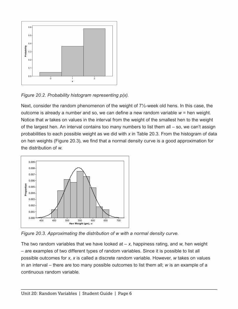
Unit 20: Random Variables | Student Guide | Page 6
210
0.6
0.5
0.4
0.3
0.2
0.1
0.0
x
Prob
abili
ty
Figure 20.2. Probability histogram representing p(x).
Next, consider the random phenomenon of the weight of 7½-week old hens. In this case, the outcome is already a number and so, we can define a new random variable w = hen weight. Notice that w takes on values in the interval from the weight of the smallest hen to the weight of the largest hen. An interval contains too many numbers to list them all – so, we can’t assign probabilities to each possible weight as we did with x in Table 20.3. From the histogram of data on hen weights (Figure 20.3), we find that a normal density curve is a good approximation for the distribution of w.
700650600550500450400
0.009
0.008
0.007
0.006
0.005
0.004
0.003
0.002
0.001
0.000
Hen Weight (gm), w
Prop
ortio
n
Figure 20.3. Approximating the distribution of w with a normal density curve.
The two random variables that we have looked at – x, happiness rating, and w, hen weight – are examples of two different types of random variables. Since it is possible to list all possible outcomes for x, x is called a discrete random variable. However, w takes on values in an interval – there are too many possible outcomes to list them all; w is an example of a continuous random variable.

Unit 20: Random Variables | Student Guide | Page 7
Let’s take a look at another discrete random variable. Table 20.4 gives a probability distribution for family size, y, in the United States. (Although there are some families that are bigger than 8, the likelihood is so small that we ignored them in this probability distribution model.)
y 1 2 3 4 5 6 7 8p(y) 0.15 0.23 0.19 0.23 0.12 0.05 0.02 0.01
Table 20.4. Distribution of U.S. family size.
From the probability distribution for y, we can find the probability that a randomly selected family will consist of at least two people using the Complement Rule:
P(y ≥ 2) = 1−P(y < 2) = 1− p(1) = 0.85
We can use the Addition Rule to find the probability that a randomly selected family will have two to four members:
P(2 ≤ y ≤ 4) = P(y = 2 or y = 3 or y = 4) = p(2)+ p(3)+ p(4) = 0.65
We can do more with probability distributions of discrete random variables than just compute probabilities. We can calculate the random variable’s mean and standard deviation. All that’s needed are the following formulas:
µ = x ⋅p(x)∑σ 2 = (x − µ)2∑ ⋅p(x) and σ = σ 2
First, we calculate the mean family size. For the calculation, multiply each outcome by its probability and then sum the results:
µ = 1× 0.15 + 2× 0.23 + 3 × 0.19 + 4 × 0.23 + 5 × 0.12+ 6 × 0.05 + 7 × 0.02+ 8 × 0.01
µ = 3.22
Next, we calculate the variance. For this calculation, multiply each outcome’s squared deviation from the mean by its probability and then sum the results:
σ 2 = (1− 3.22)2(0.15)+ (2− 3.22)2(0.23)+ . . .+ (8 − 3.22)2(0.01)
σ 2 ≈ 2.512
To get the standard deviation, take the square root of the variance:
σ ≈ 2.512 ≈1.58
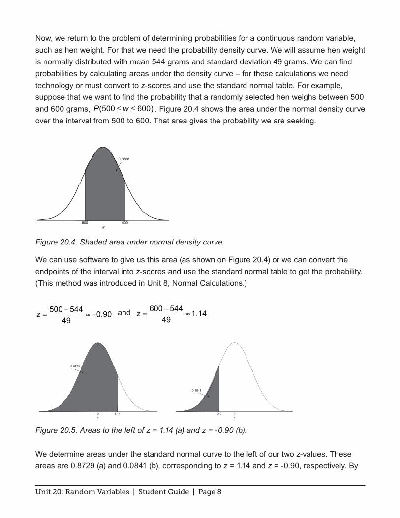
Unit 20: Random Variables | Student Guide | Page 8
Now, we return to the problem of determining probabilities for a continuous random variable, such as hen weight. For that we need the probability density curve. We will assume hen weight is normally distributed with mean 544 grams and standard deviation 49 grams. We can find probabilities by calculating areas under the density curve – for these calculations we need technology or must convert to z-scores and use the standard normal table. For example, suppose that we want to find the probability that a randomly selected hen weighs between 500 and 600 grams, (500 600)P w≤ ≤ . Figure 20.4 shows the area under the normal density curve over the interval from 500 to 600. That area gives the probability we are seeking.
w500
0.6888
600
Figure 20.4. Shaded area under normal density curve.
We can use software to give us this area (as shown on Figure 20.4) or we can convert the endpoints of the interval into z-scores and use the standard normal table to get the probability. (This method was introduced in Unit 8, Normal Calculations.)
500 544 0.9049
z −= ≈ − and
600 544 1.14
49z −= ≈
Figure 20.5. Areas to the left of z = 1.14 (a) and z = -0.90 (b).
We determine areas under the standard normal curve to the left of our two z-values. These areas are 0.8729 (a) and 0.0841 (b), corresponding to z = 1.14 and z = -0.90, respectively. By
z
0.8729
0 1.14z
-0.9
0.1841
0

Unit 20: Random Variables | Student Guide | Page 9
subtracting these two areas, we get the area under the standard normal curve over the interval from -0.90 and 1.14:
0.8729 – 0.1841 = 0.6888.
This gives us the same value that we obtained using software in Figure 20.4.
Statisticians can also compute the mean and variance of a continuous random variable. All that’s needed is a formula for the probability density curve and some calculus. The need for calculus puts computing the mean and variance of continuous random variables outside of the scope of this course.

Unit 20: Random Variables | Student Guide | Page 10
Key Terms
A random variable is a variable whose possible values are numbers associated with outcomes of a random phenomenon.
A discrete random variable can take on only a countable number of distinct values – in other words, it is possible to list its possible values. Any random variable that can take on only a finite number of values is a discrete random variable. A continuous random variable can take on values in an interval.
The probability distribution of a discrete random variable x is a list of its possible values together with the probabilities associated with those values. The probability distribution is a model for the population distribution. The random variable’s mean and standard deviation are computed as follows:
µ = x ⋅p(x)∑
σ 2 = (x − µ)2∑ ⋅p(x) ; σ = σ 2

Unit 20: Random Variables | Student Guide | Page 11
The Video
Take out a piece of paper and be ready to write down answers to these questions as you watch the video.
1. For the tossing-four-coins experiment, x was defined to be the number of heads. What are the possible values for x?
2. Given the probability distribution for x, what is the sum of the probabilities?
3. Based on the probability histogram, what is the most likely number of heads to come up in a string of four coin tosses?
4. What was the most likely cause of the Challenger disaster?
5. What rule of probability was used to find p(0), the probability that none of the six independent field joints failed?
6. What is the relationship between the probability that none of the field joints failed and the probability that at least one of the field joints failed?

Unit 20: Random Variables | Student Guide | Page 12
Unit Activity: Children in Households and School Lunch
The U.S. government collects data on many variables having to do with households. In this activity, you will examine issues related to the number of children in households and participation in free school lunch programs.
1. Whether or not a household has children is a random phenomenon. From this random phenomenon we define random variable µ as follows:
0, if no children in household 1, if at least one child in household
u =
The probability distribution of µ is given below. We have chosen to express the table with columns for the values of µ and corresponding values of p(µ). This will help with computation of mean and standard deviation later in this activity.
u p(u)0 0.5861 0.432
Table 20.5. Probability distribution of µ.
a. Draw a probability histogram for the probability distribution of u.
b. The balance point of the probability histogram is the mean, µu , of the random variable u. Based on the probability histogram from (a), do you think the balance point of this distribution is less than 0.5, at 0.5, or above 0.5? Explain.
c. Next, we walk you through one method of calculating µu = u ⋅p(u)∑ . Make a copy of Table 20.6. Enter the products of the entries from the first two columns into the third column. Then compute the sum of the entries in the third column to get µu .

Unit 20: Random Variables | Student Guide | Page 13
u p(u) (u)(p(u))
0 0.586 1 0.432
Sum = Table 20.6. Method for calculating µu .
d. You should have gotten µu = 0.432 for (c). (If not, go back and redo part (c).) Next, we walk you through one method of calculating the variance: σ u
2 = (u − µu )2 ⋅p(u) . Then you can
calculate the standard deviation by taking the square root of the variance. Make a copy of Table 20.7.
• In column three, enter the squared difference between the values of µ and µ u
• In column four, multiply the squared deviations by their corresponding probabilities.
• Sum column four to get σ u2 .
• Take the square root of σ u2 to get the standard deviation.
u p(u) (u - 0.432)^2 ((u – 0.432)^2)(p(u))
0 0.586 1 0.432
Sum =
Table 20.7. Method for calculating σ u2 .
2. In households with children, some of the school age children ate school lunches and others did not. Hence, we have another random phenomenon. Define a new random variable v as follows:
0, if none of the children in household ate school lunch 1, if at least one child in household ate school lunch
v =
a. Table 20.8 contains data collected from a U.S. government survey on random variable v. Calculate the proportions for the outcomes of v and enter them as estimates in the Probability column. Round probabilities to three decimals.

Unit 20: Random Variables | Student Guide | Page 14
v Frequency Probability0 32,491 1 74,690
Total Table 20.8. Data on random variable v.
b. Draw a diagram that represents all households broken down by whether or not there are children in the household, and then broken down further by whether or not at least one child in the household ate school lunch. Determine the proportion of all households that had at least one child who ate school lunch.
3. To ensure that children don’t go hungry, some of the children who eat school lunches get free lunches. Define random variable x as follows:
0, if household in which children ate school lunch, none got it free 1, if household in which children ate school lunch, at least one got it free
x =
The probability distribution for x is given in Table 20.9.
x p(x)0 0.4321 0.568
Table 20.9. Probability distribution of x.
From question 2, we know that 74,690 households in the survey had a least one child who ate school lunch. Estimate the number of those households in which at least one child participated in the free lunch program.
4. Next, for those households with at least one child participating in the free lunch program, some households have multiple children participating in the program. Define random variable y as follows:
y = the number of children in the household participating in the free lunch program
The probability distribution for y is given in Table 20.10.
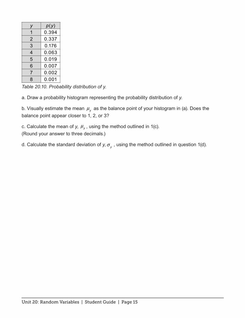
Unit 20: Random Variables | Student Guide | Page 15
y p(y)1 0.3942 0.3373 0.1764 0.0635 0.0196 0.0077 0.0028 0.001
Table 20.10. Probability distribution of y.
a. Draw a probability histogram representing the probability distribution of y.
b. Visually estimate the mean µy as the balance point of your histogram in (a). Does the balance point appear closer to 1, 2, or 3?
c. Calculate the mean of y, µy , using the method outlined in 1(c). (Round your answer to three decimals.)
d. Calculate the standard deviation of y,σ y , using the method outlined in question 1(d).

Unit 20: Random Variables | Student Guide | Page 16
Exercises
1. The random variable x, defined below, gives the average grade of 12th grade students in U.S. high schools. The probability distribution for x is given in Table 20.11.
4, if A average3, if B average2, if C average1, if D average
x
=
x 1 2 3 4p(x) 0.01 0.15 0.49 0.35
Table 20.11. Probability of grade averages.
a. Find ( 3)P x ≥ , the probability that a randomly selected student has a B or better average.
b. Find ( 3)P x < , the probability that a randomly selected student has a below B average. How is this probability related to your answer to (a)?
c. Make a probability histogram for the distribution of x. What does your graphic display tell you about the distribution of average grades?
2. The U.S. government collects data on many variables having to do with households. Let x = the number of children under 15 in a household. The probability distribution for x is shown in Table 20.12.
x 0 1 2 3 4 5 6 7 8p(x) 0.468 0.200 0.199 0.087 0.031 0.009 0.003 0.002 0.001
Table 20.12. Probability distribution for x.
a. What is the probability that a randomly selected household has at least one child under 15?
b. What is the probability that a randomly selected household has between two and four children under 15? In other words, find (2 4)P x≤ ≤ .
c. Draw a probability histogram that represents the probability distribution shown in Table 20.12. Describe the shape of the histogram.

Unit 20: Random Variables | Student Guide | Page 17
d. What is the mean number of children under 15 per U.S. household? Show your calculations.
3. A DVD manufacturer receives certain components in lots of four from two different distributors. Let x and y represent the number of defective components in each lot from Distributor 1 and Distributor 2, respectively. The probability distributions for x and y are given in Tables 20.13.
x or y p(x) p(y)0 0.40 0.151 0.33 0.702 0.18 0.153 0.05 04 0.04 0
Table 20.13. Probability distributions of x and y.
a. Draw probability histograms for the probability distributions of x and y (Table 20.13).
b. Find the mean number of defects in lots of four for both distributors. In other words, find the mean values of both x and y.
c. Find the standard deviations of x and y. Show your calculations.
d. Given the results in (b) and (c), which distributor should the DVD manufacturer rely on more heavily? Explain.
4. Assume that the distribution of weight for 7½-week old hens is normally distributed with mean 544 grams and standard deviation 49 grams. Let w = weight of a randomly selected hen.
a. Sketch normal density curve representing the distribution of w.
Use technology or the standard normal table to find the probabilities in (b) – (d). On a copy of the normal density curve that you sketched for (a), shade the area under the curve that represents each probability.
b. ( 500)P w <
c. ( 580)P w ≥
d. (500 580)P w≤ ≤
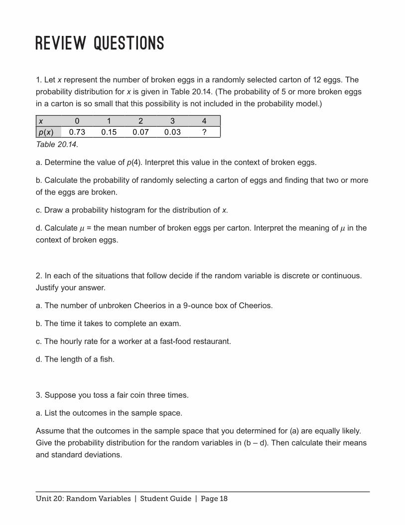
Unit 20: Random Variables | Student Guide | Page 18
Review Questions
1. Let x represent the number of broken eggs in a randomly selected carton of 12 eggs. The probability distribution for x is given in Table 20.14. (The probability of 5 or more broken eggs in a carton is so small that this possibility is not included in the probability model.)
x 0 1 2 3 4p(x) 0.73 0.15 0.07 0.03 ?
Table 20.14.
a. Determine the value of p(4). Interpret this value in the context of broken eggs.
b. Calculate the probability of randomly selecting a carton of eggs and finding that two or more of the eggs are broken.
c. Draw a probability histogram for the distribution of x.
d. Calculate µ = the mean number of broken eggs per carton. Interpret the meaning of µ in the context of broken eggs.
2. In each of the situations that follow decide if the random variable is discrete or continuous. Justify your answer.
a. The number of unbroken Cheerios in a 9-ounce box of Cheerios.
b. The time it takes to complete an exam.
c. The hourly rate for a worker at a fast-food restaurant.
d. The length of a fish.
3. Suppose you toss a fair coin three times.
a. List the outcomes in the sample space.
Assume that the outcomes in the sample space that you determined for (a) are equally likely. Give the probability distribution for the random variables in (b – d). Then calculate their means and standard deviations.

Unit 20: Random Variables | Student Guide | Page 19
b. Let x = the number of heads.
c. Let y = the absolute difference in the number of heads and tails: in other words, |number of heads – number of tails|.
d. Let w = the sum of the number of heads and tails.
4. A study of White-throated Sparrows indicates that their wingspan is normally distributed with mean 70 mm and standard deviation 3 mm. Let w = wingspan of a randomly selected White-throated Sparrow. Use technology or the standard normal table to find the probabilities in (a) – (c).
a. ( 68)P w <
b. ( 75)P w ≥
c. (68 75)P x< <

Unit 21: Binomial Distributions
Unit 21: Binomial Distributions | Student Guide | Page 1
Summary of VideoIn Unit 20, we learned that in the world of random phenomena, probability models provide us with a list of all possible outcomes and probabilities for how often they would each occur over the very long term. Probability models could be used to find out how many times we can expect to get heads on a coin toss, or how many daffodils we can expect to bloom in the spring given the number of bulbs planted in the fall, or even the number of children in a family that will have inherited a genetic disease.
There is a common thread to all of these examples. They are all concerned with random phenomena that have only two possible outcomes: heads versus tails, blooms versus none, sick versus healthy. Traditionally, we label one possible outcome as a success and the other as a failure. In this unit, what we are interested in is the number of successes. This count forms a particular kind of discrete probability model called the binomial distribution.
In addition to a situation having only two possible outcomes, there are three more conditions that must be true in order for it to be in a binomial setting. To demonstrate all four conditions, we turn to the context of basketball free throws. Free throws are mostly clear of any defensive pressure or other external factors during a basketball game. We only need to be concerned with whether or not the ball goes into the net.
The first trait of a binomial setting is that there is a repeated, fixed number, n, of trials, or observations. In this case, n equals the number of shots taken. Second, all of these trials are independent; meaning that the outcome of one trial does not change the probabilities of the other trials. Now, conventional basketball wisdom might tell you this is not true if a player has a “hot hand,” meaning that, because of the success of their previous shots, they are more likely to make successive baskets. But a 1985 study showed that this was not the case. The study found that players are not more likely to make second shots after making their first. The second shot’s outcome is independent of the first shot. Therefore, free throws do fit this trait of a binomial setting. The third trait that we must look at is whether or not each of the trials ends in one of two outcomes: success, S, or failure, F. Our basketball example fits – either the ball goes into the net (success) or it misses (failure). Lastly, the probability of success, or

Unit 21: Binomial Distributions | Student Guide | Page 2
p, must be the same for all trials. Free throws are always shot from the same distance. There is no defensive pressure. Each time the player lines up at the free throw line he has the same probability of making his shot, which is based on his particular shooting skills. So, basketball free throws fit the binomial setting!
Next, we look at an example where the binomial setting comes up in genetics. Binomial distributions can help determine the probability of how many children in a family of six will inherit a genetic disease. Sickle cell disease is a genetic disorder of the red blood cells, estimated to affect around 100,000 people in the United States. It can cause a great deal of pain, life-threatening infections, strokes, and chronic organ damage. Inside the red blood cells is a protein called hemoglobin. There are different types of hemoglobin. For example, in the womb we all have fetal hemoglobin or hemoglobin F. After birth, we change over to normal hemoglobin A or, for people with sickle cell disease, to hemoglobin S. Like all genetic traits, the genes that determine an individual’s hemoglobin type are inherited, one version from each parent. Since sickle cell is a recessive disease, a child needs to receive two bad versions of the gene, one from each parent, to have the disease.
In the typical situation for two parents who are carriers, each has one bad copy of the gene, S, and one good copy, A. Each time the mother makes an egg, there is a 50% chance that she will produce an egg that has the sickle mutation and a 50% chance she will produce a normal egg. On the other side, the father has a 50% chance that his sperm will have the sickle mutation and a 50% chance of normal. When the sperm and egg come together there are four possible outcomes for the gene from the mother and gene from the father (in that order): AA, AS, SA, SS. So, there is a 25% chance of the child inheriting SS and thus having the disease and a 75% chance of the child inheriting something other than SS and not having the disease. Because of the parents’ genetic makeup, this probability never changes. With each pregnancy the probability of having a child with sickle cell disease is 1/4 or 0.25. So sickle cell disease fits the binomial setting. Here’s a recap of why:
There are two possible outcomes – a sick child or a healthy child.
For this family, there are six children; n = 6.
The outcome for each child is independent.
The parents’ genetic makeup never changes; p = 0.25 for each child.
Next, we look at a probability histogram for the number of children with sickle cell disease in families with six children where each parent is a carrier. We can use technology or a binomial table to calculate the probabilities and then use the values to form the histogram (See Figure 21.1.). The horizontal axis is marked with the values for x, the number of sick children in a

Unit 21: Binomial Distributions | Student Guide | Page 3
family of six children. The vertical axis shows the probability for each possible value of x.
Figure 21.1. Probability histogram for a binomial distribution; n = 6 and p = 0.25.
We can see from this histogram that the probability of having three children with sickle cell, for example, is around 0.13 or 13%.
Public health officials might want to find the mean of this distribution. Fortunately that is easy to calculate. We just multiply the number of trials, n, times the probability of success, p:
μ = np
So, the mean number of children with sickle cell disease, in families of six children, where both parents are carriers, is 1.5. Of course, no family has 1.5 children! This is the statistical average over many, many families.

Unit 21: Binomial Distributions | Student Guide | Page 4
Student Learning Objectives
A. Be able to identify a binomial setting and define a binomial random variable.
B. Know how to find probabilities associated with a binomial random variable.
C. Know how to determine the mean and standard deviation of a binomial random variable.

Unit 21: Binomial Distributions | Student Guide | Page 5
Content Overview
A basketball player shoots eight free throws. How many does he make? In a family of six children with two parents who are carriers of a genetic disease, how many of their children will inherit the disease? If you throw two dice four times, how many times will you throw doubles? In each of these situations, we can identify an outcome that we would like to count. We label that outcome a success (even if, as in the case of children inheriting a disease, that outcome is not good) and any other possible outcomes from these random phenomena as failure. So we begin our discussion with random phenomena in which all possible outcomes can be classified into one of two categories, success or failure.
In settings in which we can classify outcomes into successes and failures, we can define a random variable x to be the number of successes. The random variable x has a binomial distribution if the conditions of a binomial setting are satisfied. Those conditions are listed below.
The Binomial Setting
1. There is a fixed number of n trials or observations.
2. The trials are independent.
3. The trials end in one of two possible outcomes: Success (S) or Failure (F).
4. The probability of success, p, is the same for all trials.
If the conditions of the binomial setting are satisfied, then x, the number of successes, has a binomial distribution with parameters n and p; we express this distribution in shorthand as b(n, p).
Now, we look at an example. As of August 2013, Jacqui Kalin was listed as having the top free throw percentage in Women’s NCAA basketball. Her percentage of successful free throws was 95.5%. Suppose we test her skills on the basketball court and ask her to throw 20 free throws. Our random variable x is the number of free throws that she makes and we have a fixed number of n = 20 free throws. From the video, we know that consecutive free throws are independent. Each free throw either goes into the basket (success) or does not (failure). The probability of success depends on the shooting skills of the player; for Jacqui, p = 0.955. So, x, the number of successful free throws out of 20, fits the binomial setting and the distribution of x is b(20, 0.955).

Unit 21: Binomial Distributions | Student Guide | Page 6
Number 50 on the 2013 list of the highest free throws percentages in Women’s NCAA basketball is Lauren Lenhardt. Her free throw percentage was listed as 83%. Suppose we test her skills on the basketball court and ask her to throw free throws until she gets a basket. We let y be the number of free throws until she gets one in the hoop. Unlike random variable x in the previous paragraph, y is not a binomial random variable because there is no fixed number of trials. If she makes her first free throw, then she stops and n = 1. If she misses and makes her second free throw, then n = 2.
One typical setting for the binomial distribution is with simple random samples.
Suppose that of the 2,500 adult patients at a healthcare center, 750 have high blood pressure and 1,750 do not have high blood pressure. Suppose that we select a random sample of 5 patients from the health center and let x equal the number of patients who have high blood pressure. This is not quite a binomial setting. Here’s why. For trial 1, we randomly choose the first patient. The probability that Patient 1 has high blood pressure is 750/2500 = 0.3. Now, for trial 2 we have 2,499 patients to choose from. The probability that Patient 2 has high blood pressure depends on the outcome for Patient 1. If Patient 1 had high blood pressure, then the probability that Patient 2 has high blood pressure is 749/2499 ≈ 0.2997. But if Patient 1 does not have high blood pressure, then the probability that Patient 2 has high blood pressure is 750/2499 ≈ 0.3001. So, the probability of success, having high blood pressure, is not constant for each trial. However, in this case, the distribution of x will be very close to b(5, 0.3). We summarize this result as follows.
Choose a simple random sample of size n from a population with proportion p of successes. Let x be the number of successes in the sample. If the population is much larger than the sample, then x’s distribution is approximately b(n, p). (A good rule of thumb is that the population must be at least 20 times larger than the sample.)
Next, consider the context of children inheriting blue eyes from their brown-eyed parents, each of whom has a recessive gene for blue eyes. We’ll label inheritance of blue eyes as success. In this case, each of their children has a 25% chance of inheriting blue eyes. In a family of six children whose parents have this genetic makeup, we would like to find the probability distribution for the number of their children, x, who will have blue eyes. In this situation, the distribution of x is b(6, 0.25).
Step 1: Find p(0).
When x = 0, that means all six trials were failures: FFFFFF. From the Complement Rule, we know that P(F) = 1 – P(S) = 0.75. Since the trials are independent, we can use the Multiplication Rule to find the probability:

Unit 21: Binomial Distributions | Student Guide | Page 7
p(0) = P(FFFFFF) = (P(F))6 = (0.75)6 ≈ 0.178
Step 2: Find p(1).
When x = 1, one of the six trials is a success and the other five are failures. There are six possible ways that could happen:
SFFFFF, FSFFFF, FFSFFF, FFFSFF, FFFFSF, FFFFFS
We use the Multiplication Rule to find the probability that any outcome with one success and five failures occurs: (0.25)(0.75)5, and there are six of these outcomes:
p(1) = 6(0.25)(0.75)5 ≈ 0.336
Step 3: Find p(2).
When x = 2, two of the six trials are a success and the other four are failures. There are 15 possible ways that could happen:
SSFFFF, SFSFFF, SFFSFF, SFFFSF, SFFFFS,
FSSFFF, FSFSFF, FSFFSF, FSFFFS, FFSSFF,
FFSFSF, FFSFFS, FFFSSF, FFFSFS, FFFFSS
We use the Multiplication Rule to find the probability that any outcome with two success and four failures occurs: (0.25)2(0.75)4 and there are 15 of these outcomes:
p(2) = 15(0.25)2(0.75)4 ≈ 0.297
At this point we could keep going and finish finding the probability distribution for x. However, our calculations to this point can serve as a pattern for a formula. First, we need to count the number of ways there are x successes in six trials. We can do that with combinations:
6x
⎛
⎝⎜⎞
⎠⎟= 6!x!(6 − x)! is the number of ways to choose x trials to label S from 6 trials.

Unit 21: Binomial Distributions | Student Guide | Page 8
In the case of x = 2:
62
⎛
⎝⎜⎞
⎠⎟= 6!2!4!
= 6 ⋅5 ⋅4!2!4!
= 15
Step 4: Find p(3). Following the pattern established with p(0), p(1), and p(2), we get:
p(3) = 63
⎛
⎝⎜⎞
⎠⎟0.25( )3 0.75( )3 = 6!
3!3!0.25( )3 0.75( )3 = 20(0.25)3(0.75)3 ≈ 0.132
The general formula for calculating binomial probabilities is contained in the box below.
Binomial Probability
If the distribution of x is b(n, p), then the probabilities associated with x are given by
p(x) = nx
⎛
⎝⎜⎞
⎠⎟px 1− p( )n−x for x = 0, 1, 2, . . . , n.
Now that we can find the probability distribution for any binomial random variable, we could use the formulas given in Unit 20, Random Variables, to calculate its mean and standard deviation. However, there is a much easier way to calculate the mean and standard deviation when dealing with binomial random variables.
Mean and Standard Deviation
If the distribution of x is b(n, p), then the mean and standard deviation of x are
µ = np
σ = np(1− p)
So, for example, given x that is b(6, 0.25), the mean and variance of x are:
μ = (6)(0.25) = 1.5
σ = (6)(0.25)(0.75) = 1.125 ≈1.06

Unit 21: Binomial Distributions | Student Guide | Page 9
We conclude this overview with one interesting feature of binomial distributions. Suppose we leave p at a fixed value and then allow n to increase – say from 5 to 30. Figure 21.2 shows histograms for the following distributions:
b(5, 0.3) (top left)
b(10, 0.3) (top right)
b(20, 0.3) (bottom left)
b(30, 0.3) (bottom right)
Notice that the probability histogram for b(5, 0.3) is skewed to the right. However, as n increases to 30, the probability histograms look more and more like bell-shaped curves. This example shows that if x has a binomial distribution and n is large, then we can approximate its distribution with a normal distribution.
Figure 21.2. Probability histograms of four binomial distributions
Normal Approximation for Binomial Distributions
If x has the distribution b(n, p) and n is large, then the distribution of x is approximately normal with mean μ = np and standard deviation σ = np(1− p) . As a rule of thumb, this is a good approximation as long as n is sufficiently large so that np ≥10 and n(1− p) ≥10 .
15129630
0.4
0.3
0.2
0.1
0.0
15129630
0.4
0.3
0.2
0.1
0.0
b(5, 0.3)
Prob
abili
ty
b(10, 0.3)
b(20, 0.3) b(30, 0.3)
Unit 21: Binomial Distributions | Student Guide | Page 10
Key Terms
In a binomial setting, there is a fixed number of n trials; the trials are independent; each trial results in one of two outcomes, success or failure; the probability of success, p, is the same for each trial. In a binomial setting with n trials and probability of success p, x = the number of successes that has the binomial distribution with parameters n and p. Shorthand notation for this distribution is b(n, p).
Probabilities for random variable x that has the distribution b(n, p) can be calculated from the following formula:
p(x) = nx
⎛
⎝⎜⎞
⎠⎟px(1− p)n−x for x = 0, 1, . . . n,
where nx
⎛
⎝⎜⎞
⎠⎟= n!x!(n − x)!
.
The mean and standard deviation of binomial random variable x can be calculated as follows:
µ = np
σ = np(1− p)

Unit 21: Binomial Distributions | Student Guide | Page 11
The Video
Take out a piece of paper and be ready to write down answers to these questions as you watch the video.
1. In a random phenomenon with only two possible outcomes, traditionally what terms are used to label the two outcomes?
2. Give some reasons why the probability of success, p, for free throws is the same for each trial.
3. What is the probability of inheriting sickle cell disease for a child with two parents who are carriers? Why is this probability the same for each child in the family?
4. What is the formula for calculating the mean of a binomial random variable?
5. List the four conditions needed for a binomial distribution.

Unit 21: Binomial Distributions | Student Guide | Page 12
Unit Activity: Inheriting a Genetic Disease
Each person has two copies of the eye color gene in their genome, one inherited from each parent. Let B stand for brown and b stand for blue. Brown is the dominant color, which means that a person with eye color genes Bb (B from mother and b from father) will have brown eyes. If brown eyed parents each have the recessive gene for blue eyes, b, then each of their children will have a 25% chance of having blue eyes, or genes bb.
In this activity, you will simulate the prevalence of blue eyes in families of four children, in which both parents have brown eyes but carry a recessive gene for blue eyes. We label the outcome as success if a child has blue eyes – not because blue eyes are better than brown, but because that is the outcome we are counting. In this case, the probability of success is p = 0.25.
For this activity, you will need to simulate selecting 30 samples of families with four children where both parents have brown eyes but have a recessive gene for blue eyes. If your instructor does not provide you with a method to simulate samples of four-children families, use one of the following methods:
Method 1: You will need two coins of different denominations, say a nickel and a quarter. Let the nickel represent the gene the child inherits from the mother – if heads, the child receives gene b and if tails, gene B. Then let the quarter represent the gene that the child inherits from the father – if heads, the child receives gene b and if tails, gene B. Flip the two coins, if both land heads, then the child will inherit blue eyes and the outcome is labeled a success.
Method 2: Generate a random number from the interval from 0 to 1. Excel’s Rand() will work for this. If the number is 0.25 or less, call it a success. If the number is above 0.25 call it a failure.
You will generate outcomes for four children in a family. Each child is a new trial that ends in success, blue eyes, or failure, brown eyes. This process will be repeated 30 times. Save your data for use in Unit 28, Inference for Proportions.
1. In a copy of Table 21.1, record an S for each trial for which the child inherits blue eyes and an F for each trial for which the child inherits brown eyes. Let x be the number of successes in the family. Record the value of x for each family.

Unit 21: Binomial Distributions | Student Guide | Page 13
2. a. In a copy of Table 21.2, construct a relative frequency distribution for the number of successes in four trials. In the second column, enter the number of times 0, 1, 2, 3, and 4 successes were observed. In the third column, enter the proportion (relative frequency) of times 0, 1, 2, 3, and 4 successes were observed.
b. In the fourth column, enter the probabilities. To find these probabilities, you can use statistical or spreadsheet software, a graphing calculator, or an online binomial calculator. (You could also use the formulas from the Content Overview.)
3. a. Display the x-data in a histogram. Use proportion for the scaling on the vertical axis.
b. Represent the probability distribution with a probability histogram.
c. Compare your graphs from (a) and (b).
4. In a second copy of Table 21.2, combine the data from the class.
a. Display the x-data from the class in a histogram. Use proportion for the scaling on the vertical axis.
b. Compare your histogram in (a) to the probability histogram you drew for 3(b).

Unit 21: Binomial Distributions | Student Guide | Page 14
Table 21.1. Outcomes for each family of four children.
Trial #Sample 1 2 3 4 x
123456789
101112131415161718192021222324252627282930
Table 21.1
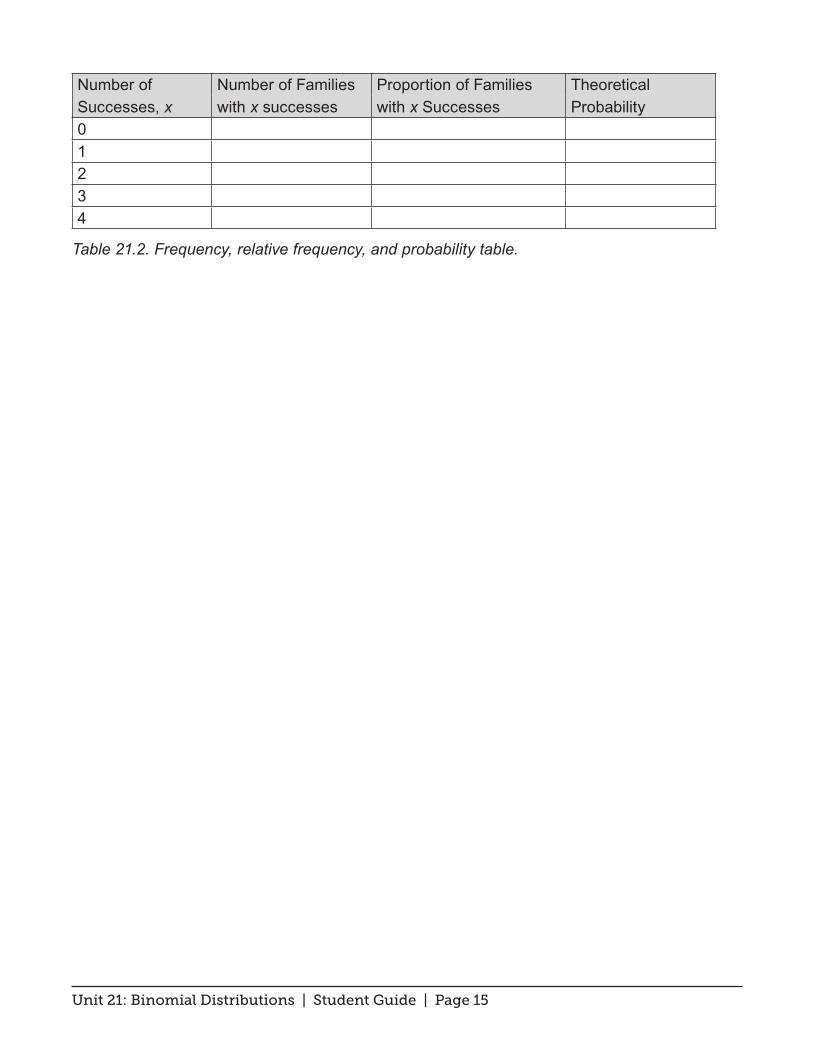
Unit 21: Binomial Distributions | Student Guide | Page 15
Number of Number of Families Proportion of Families TheoreticalSuccesses, x with x successes with x Successes Probability0 1 2 3 4
Table 21.2. Frequency, relative frequency, and probability table.

Unit 21: Binomial Distributions | Student Guide | Page 16
Exercises
1. Decide if each of the following situations fits the binomial setting. Give reasons for your answer in each case. If x has a binomial distribution, state the values of n and p.
a. Roll a fair die until it comes up six. Let x be the number of rolls needed to get the six.
b. Roughly 60% of Americans believe that extraterrestrial life exists on other planets. A random sample of 10 Americans is selected and during phone interviews are asked their opinion on extraterrestrial life. Let x be the number who say they believe in extraterrestrial life.
c. A deck of cards is shuffled. You draw a card and check to see if it is a red card and then put it aside. Then you draw a second card and check to see if it is a red card and put it on top of the first card drawn. You continue until you have drawn 5 cards. Let x be the number of red cards in the five that were drawn.
2. Blood banks are happy to receive blood donations from people who are type O+ (O positive) and O- (O negative). All people with Rh-positive blood can receive an O+ blood transfusion. The probability of having type O+ blood is 0.374. Suppose a random sample of four people show up during a blood drive to donate blood. Let x be the number of people with blood type O+.
a. Use the formulas given in the Content Overview to create a probability distribution table for x. Show your calculations. Round probabilities to two decimals.
b. In Unit 20, Random Variables, you learned how to calculate the mean of a discrete random variable: µ = x ⋅p(x)∑ . Use this formula to compute the mean number of people with type O+ blood in a random sample of size four.
c. From this unit, you have learned another way to calculate the mean of binomial random variables: µ = np . Use this formula to compute the mean. Compare your answer with your results in (b). Explain why there might be a slight discrepancy between your two answers.
d. Make a probability histogram to represent the probability distribution of x. Mark the mean, μ, on the horizontal axis.

Unit 21: Binomial Distributions | Student Guide | Page 17
3. Let w, x, and y be random variables with binomial distributions with n = 5 and probability of success p. Let p = 0.2 for w, p = 0.5 for x, and p = 0.8 for y.
a. Create probability distribution tables for w, x, and y. (Use software or tables to find the probabilities.)
b. Find the mean and standard deviation for each of the three distributions.
c. Draw probability histograms for the distributions of w, x, and y. Use the same scaling on all three histograms.
d. Compare the shapes of the three histograms. In two cases, the standard deviations of the random variables are the same (see solution (b)). Give an explanation based on the histograms for why that should be the case.
4. A drug manufacturer claims that its flu vaccine is 85% effective; in other words, each person who is vaccinated stands an 85% chance of developing immunity. Suppose that 200 people are vaccinated. Let x be the number that develops immunity.
a. What is the distribution of x?
b. What is the mean and standard deviation for x?
c. What is the probability that between 165 and 180 of the 200 people who were vaccinated develop immunity? (Hint: Use a normal distribution to approximate the distribution of x.)

Unit 21: Binomial Distributions | Student Guide | Page 18
Review Questions
1. Decide if each of the following situations fits the binomial setting. Give reasons for your answer in each case. If x has a binomial distribution, state the values of n and p.
a. A random sample of 100 college students were asked: Do you routinely eat breakfast in the morning? Define x to be the number who respond Yes.
b. Classify the accidents each week into two categories, those involving alcohol and those not involving alcohol. Let x be the number of accidents involving alcohol in a week.
c. A particular type of heart surgery is successful 75% of the time. Five patients (who are not related) get this type of heart surgery. Let x be the number of successful surgeries.
2. People with O- blood are called universal donors because most people can receive an O- blood transfusion. The probability of having blood type O- is 0.066. Suppose a random sample of five people show up during a blood drive to donate blood. Let x be the number of people with blood type O-.
a. What is the probability that none of the five people has blood type O-? Show your calculations.
b. What is the probability that exactly one of the five has blood type O-? Show your calculations.
c. What is the probability that no more than one of the five people has blood type O-?
d. What is the probability that at least one of the five has blood type O-?
3. Let x be the number of children who have sickle cell disease in a family with three children, in which each parent is a carrier. Recall from the video that each child has a probability of 0.25 of having the disease.
a. Calculate the probability of each possible value of x. Round probabilities to two decimals.
b. Find the mean number of children who have the disease in families with 3 children where both parents are carriers. Interpret the value that you calculate in the context of this problem.

Unit 21: Binomial Distributions | Student Guide | Page 19
c. Draw a probability histogram for this distribution. Mark the location of the mean on your histogram.
4. According to the Centers for Disease Control and Prevention (CDC), 31% of American adults have high blood pressure. Suppose a random sample of 100 Americans is selected. Let x be the number with high blood pressure.
a. What is the distribution of x?
b. What is the mean and standard deviation of x?
c. What is the probability that fewer than 25 people in the sample have high blood pressure? Explain how you arrived at your answer.