Unit 2

Market Demand, Supply,

And Prices

Input Suppliers to Cut Production

Sam, the CEO of PC Solutions, recently read a WSJ article that quoted executives of Samsung and of Hyundia indicating those companies would be reducing their production of PC memory chips. The article went on to say a third company, LG Semicon, would likely follow suit. Collectively, these three companies produce about one-third of the world’s basic semiconductor chips. As part of their operations, PC Solutions buys PC memory chips. The company is relatively small but has been growing (e.g. 100% last year) and is in the process of deciding whether or not to double its workforce. Should PC Solutions’ plans be impacted by the WSJ article?

Using S & D Projections

Sue, a commodity merchandiser for KonAgra, is aware that the current market price of a commodity she trades is $1.50 per unit. Her company has just projected for this commodity a new near-term market supply of P = .01Q and market demand of P = 4 - .01Q. What should she expect to happen to the price of this commodity near term? Should her merchandising actions be impacted by this new, updated information?

A Shortage?

In recent years, there has been a significant increase in the amount of corn-based ethanol produced in the state of Iowa. As a result, numerous popular press articles have questioned whether or not the state will see a “shortage” of corn production. What would this mean and is it likely to happen?

Curing Hunger with Cheap Food Prices?

In recent years, Zimbabwe’s government has imposed price controls on many basic commodities, including food. What does this mean and what are your predicted impacts of these price controls on food production and food trade, as well as on hunger and malnutrition in Zimbabwe?

Demand of Microsoft’s Dos

In the late 1970’s, Microsoft developed the DOS operating system, initially designed for IBM computers. Microsoft pursued a relatively low pricing strategy for its DOS product to encourage consumers to buy more ‘DOS” computers. Were there any other controllable factors that Microsoft used to its advantage to increase the demand for its product?

S & D Managerial Implications

Understand how P’s are determined in order to anticipate P changes

Understand how P changes impact consumers & producers (i.e. coordinate economic activities)

Understand how to capitalize on anticipated P changes

• buying• selling• producing

• maintaining inventory• contracting• staffing

Why Prices are Important to Firms

1. Influence $ sales if a firm is a seller

e.g. total revenue = TR = P Q

2. Influence $ expenses if a firm is a buyer

e.g. Total cost = TC = P Q

=> Firms want to “Buy low, sell high”!

Market Demand Curve

Shows the amount of a good that will be purchased at alternative prices.

Law of Demand– The demand curve is downward sloping.

Demand Curves are associated with a given:

1. Product (specified ‘dimensions’)→ quality or type→ location→ time period

2. Number of buyers→ one consumer/buyer→ all customers of a given firm→ all customers in a given geographic area (i.e. market)

Output or Product Markets

HouseholdsD OutputsS Inputs

Input or Factor Markets

FirmsD InputsS Outputs

Note: Physical items flow clockwise; payments flow counter clockwise.

General Demand Function

An equation representing the demand curve

Q f P P M Hxd

x Y ( , , , , )

= quantity demand of good X.Q xd

Px = price of good X.

PY = price of a related good Y (substitute or

complement). M = income. H = any other variable affecting demand.

Factors That Affect D for X(controllable and non controllable)

1. Px = P of that product (or item) (note ΔP could be caused by Δ supply)2. P and/or availability of another item (e.g. Y)

a. Substitutes (↑ P => ↑ D for X)b. Complements (↑ PY => ↓ D for X)

3. Income (I)a. Inferior (↑ I => ↓ D for X)b. Normal (↑ I => ↑ D for X)

4. Type of Itema. Luxuryb. Necessity

5. Buyer concerns or expectationsa. Safety and/or healthb. Quality (warranty ?)c. Future cost/availabilityd. Service

6. Advertising7. Tastes and preferences8. No. of buyers or alternative uses9. Govt. policy (e.g. tax)10. Seasonality11. Interest rates12. Profitability of an input (i.e. = derived demand)

Specific Demand Function

Q a bP cP dM eHxd

x Y

inverse’ demand equation would be theabove equation solved for Px giventhe values of all the other demand factors

Effects of D Factor Changes

Q

PQ for each un it P b

Q

MQ for each un it M d

x

xx x

xx

1

1

Change in Demand(due to P of THAT product)

Change in Demand(Due to a other than P of THAT product)

Quote of the Day

“In this world, there are two ways to get rich:

#1. Produce something valuable and sell

it to others.

#2. Steal from those who are successful

at pursuing the first strategy.”

N. Gregory Mankiw

Fortune (June 12, ’00)

The Progression of Economic ‘Value’

Product ‘Activity’ Buyer

Commodity Extract Market

Goods Produce Customer

Services Deliver Client

Experiences Stage Guest

Transformation Guide Aspirant

Mass Customization (by Pine, ’93)

Specific D Function Example

Qx = 20 – Px + 2Py

If Py = 5,

=> Px = 30-Qx (= ‘inverse’ D function equation)

If Py = 10,

=> Px = 40-Qx

Note, an increase in the price of Y has increased The vertical axis intercept without changing the Slope of the original D curve. Thus, there has Been a parallel shift to the right of the D curve for X.

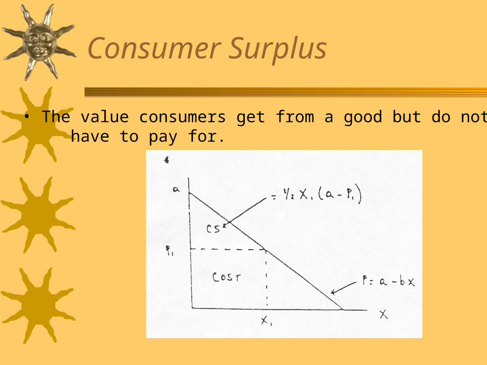
Consumer Surplus

• The value consumers get from a good but do nothave to pay for.

Market Supply Curve

The supply curve shows the amount of a good that will be produced at alternative prices.

Law of Supply– The supply curve is upward sloping.

General Supply Function

An equation representing the supply curve:

QXS=f(PX, PR, W, H,)

QXS = quantity supplied of good X.

PX = price of good X. PR = price of a related good. W = price of inputs (e.g. wages) H = other variable affecting supply

Factors that Affect S of X(controllable and non controllable)

1. Px = P of that product or item (note ΔP could be caused by ΔD)

2. P or profitability of an alternative production item (e.g. Y) (↑ PY => ↓ S of X)

3. P or cost of an input (e.g. Z) (↑ PZ => ↓ S of X)4. Taxes5. Interest rates6. Gov’t policies/regulations7. Technology8. Producer expectations9. Weather10. Number of producers

QXS = a+bPX+cPY+dW+eH

‘inverse’ supply equation would be the above equation solved for PX given the values of all the other supply factors

Specific Supply Function

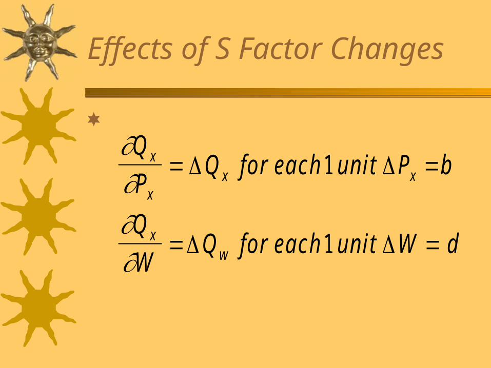
Effects of S Factor Changes

Q

PQ for each un it P b

Q

WQ for each un it W d

x

xx x

xw

1

1

Change in Supply(Due to P of THAT product)

A to B: Increase in quantity supplied

Change in Supply(Due to other than P of THAT product)

S0 to S1: Increase in supply

Specific S Function Example

QX = 2PX – W

if W = 5,

QX = 2PX – 5

PX = 2.5 + .5QX

if W = 10,

PX = 5 + .5QX

Producer Surplus

The amount producers receive in excess of the amount necessary to induce them to produce the good.

Market Equilibrium

Balancing supply and demand

QXS = QX

D

Steady-state

If price is too high . . .

If price is too low . . .

Equilibrium Price =

That price for which the amount buyers are willing and able to buy equals the amount producers are willing and able to sell

Solving for Equil P

Equil S price = D price

0 + .01Q = 4 - .01Q

.02Q = 4

Q = 200

P = 0 + .01 (200)

P = 2.00

Equilibrium Over Time

Equilibrium Changes

Case P Q

1. D 2. D 3. S 4. S 5. D, S ? 6. D, S ?

7. D, S ?

8. D, S ?

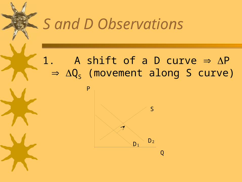
S and D Observations

1.A shift of a D curve P QS (movement along S curve)

P

S

Q

D2D1

S and D Observations

2. A shift of a S curve P QD (movement along D curve)

P

D

Q

S1S1S1

S2

S and D Observations

3. A P in ONE market may shift in S or D in ANOTHER market (e.g. all products if they become too expensive, are likely to have substitutes)

Favorite Trading Rules

“The reaction of the market to news is more important than the news itself.”

“People who buy headlines end up selling newspapers.”

“Facts are priceless – opinions are worthless.”

Rich Felthaus, Refco, July 2004

Big Picture: Impact of decline in component prices on PC market

Big Picture: Impact of lower PC prices on the software market

Market Equilibrium & NSW

NSW= net social welfare

= PS + CSMax NSW P = Pe

P

S

CS

D

Q

Pe

Qe

PS

NSW Impacts: Q & P

NSW = net social welfare

= PS + CS= (a-c) + (-a-b)= -c –b= net welfare loss (deadweight loss)

Price Restrictions

Price Ceilings– The maximum legal price that can be charged– Examples:

• Gasoline prices in the 1970s• Housing in New York City• Proposed restrictions on ATM fees

Price Floors– The minimum legal price that can be charged– Examples:

• Minimum wage• Agricultural price supports

Impact of a Price Ceiling

Impact of a Price Floor

Incidence of a Tax

Pb is the price (including the tax) paid by buyers. Ps is the price that sellers receive, net of the tax. Here the burden of the tax is split about evenly between buyers and sellers. Buyers lose A + B, sellers lose D + C, and the government earns A + D in revenue. The deadweight loss is B + C.