1

UNIT 3 Data Wrangling

2

Introduction to Data Wrangling

Data pre-processing (aka "wrangling") can be defined as the preparation of data for analysis

with data mining and visualization tools. There are many problems which can interfere with a

successful analysis; some of them can be readily addressed with simple pre-processing

techniques, which we will explore in this unit.

A range of data issues can be avoided by early planning of data collection. If data scientists

can anticipate that a study of customer satisfaction will need customer income levels, for

example, then in organizing a survey they can arrange to ask about income, whereas without

anticipating those, data scientists never think to ask and end up with poor data. Data scientists

generally have no say in the original collection of data and are simply handed a data set. Then

there are only two options at their hands: (1) wrangling with the data to reduce or eliminate

problems; (2) reporting on the problems and how to avoid them in future data collection.

It is often said that data scientists spend about 70 per cent of their time in data wrangling.

Only after that does it really make sense to do any analysis. If data scientists do not take the

time to ensure that data is in good shape before doing any analysis, they often run a big risk

of wasting a lot of time later on, or worse, losing the faith of their project stakeholders.

The most important thing to keep in mind about data cleaning, is that it's an iterative process.

Iterate on first detecting, and then correcting bad records. For example, one might have text

where we expect to find numeric data. So the word two instead of the number two. Some data

items might not be designed according to pre-defined specification. They might be missing

entire fields or they might have extra fields.

In measuring the quality of data, data scientists measure the degree to which entries in data

set conform to a defined schema, or to other constraints. They also look at accuracy. This is

the degree to which entries conform to gold standard data. Completeness of data is

straightforward i.e. do we have all the records we should have. Data consistency also is an

important aspect of data quality. Data scientists need to ensure that there is consistency

among the fields that represent the same data across systems. Finally, data uniformity, which

means whether values for distance, for example, use the same units; Is it miles, or is it

kilometres.

3

Introduction to R

Installing R and Packages R is a programming environment, which uses a simple programming language, allows for rapid

development of new tools according to user demand. These tools are distributed as packages,

which any user can download to customize the R environment. Base R and most R packages

are available for download from the Comprehensive R Archive Network (CRAN) in the

following web address:

cran.r-project.org

R packages are the fuel that drives the growth and popularity of R. R packages are bundles of

code, data, documentation, and tests that are easy to share with others.

Before one can use a package, one will first have to install it. Some packages, like the base

package are automatically installed. Other packages, like for example the ‘ggplot2’ package,

will not come with the bundled R installation but need to be installed.

Many (but not all) R packages are organized and available from CRAN, a network of servers

around the world that store identical, up-to-date, versions of code and documentation for R.

Using the ‘install.packages’ function data scientists can easily install these packages from

inside R. CRAN also maintains a set of Task Views that identify all the packages associated

with a particular task.

In addition to CRAN, data scientists also have bioconductor which has packages for the

analysis of high-throughput genomic data, as well as for example the github and bitbucket

repositories of R package developers. You can easily install packages from these repositories

using the devtools package.

R comes with several basic data management, analysis, and graphical tools. R's power and

flexibility lies in its array of packages (currently more around 6,000).

Data scientists can work directly in R, but most prefer a graphical interface. For starters:

• RStudio, an Integrated Development Environment (IDE)

• Deducer, a Graphical User Interface (GUI)

RStudio

R is the name of the programming language itself and RStudio is a convenient interface. There

a several fundamental building blocks of R and RStudio. These blocks are the interface,

running code, and basic commands.When you first launch RStudio, you will be greeted by an

interface that looks like this:

4

Insert diagram here.

The panel in the upper right contains the workspace as well as a history of the commands that

are entered. Any plots that you generate will show up in the panel in the lower right corner.

The panel on the left is the console. Each time RStudio is launched, it will have the same text

at the top of the console telling you the version of R. Below that information is the prompt

where R commands are entered. Interacting with R is all about typing commands and

interpreting the output. These commands and their syntax are the window to access data,

organize, describe, and perform statistical computations.

For the purposes of this lesson, we will be using the following packages frequently:

• ‘foreign’ package to read data files from other stats packages

• ‘readxl’ package for reading Excel files

• ‘dplyr’ package for various data management tasks

• ‘reshape2’ package to easily melt data to long form

• ‘ggplot’ and ‘ggplot’ packages for elegant data visualization using the Grammar of

Graphics

• ‘GGally’ package for scatter plot matrices

• ‘vcd’ package for visualizing and analyzing categorical data

• ‘lattice’ is a powerful and elegant high-level data visualization system

Installing R Packages

To use packages in R, let’s install them using the ‘install.packages’ function, which typically

downloads the package from CRAN.

#install.packages("foreign")

#install.packages("readxl")

#install.packages("dplyr")

#install.packages("reshape2")

#install.packages("ggplot2")

#install.packages("GGally")

#install.packages("vcd")

Loading R Packages

When data scientists need an R package for R sessions, the specific packages must be loaded

into the R environment using the ‘library’ or ‘require’ functions.

5

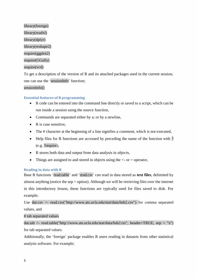
library(foreign)

library(readxl)

library(dplyr)

library(reshape2)

require(ggplot2)

require(GGally)

require(vcd)

To get a description of the version of R and its attached packages used in the current session,

one can use the ‘sessionInfo’ function;

sessionInfo()

Essential features of R programming

• R code can be entered into the command line directly or saved to a script, which can be

run inside a session using the source function,

• Commands are separated either by a; or by a newline,

• R is case sensitive,

• The # character at the beginning of a line signifies a comment, which is not executed,

• Help files for R functions are accessed by preceding the name of the function with ?

(e.g. ?require),

• R stores both data and output from data analysis in objects,

• Things are assigned to and stored in objects using the <- or = operator,

Reading in data with R

Base R functions ‘read.table’ and ‘read.csv’ can read in data stored as text files, delimited by

almost anything (notice the sep = option). Although we will be retrieving files over the internet

in this introductory lesson, these functions are typically used for files saved to disk. For

example;

Use dat.csv <- read.csv("http://www.ats.ucla.edu/stat/data/hsb2.csv") for comma separated

values, and

# tab separated values

dat.tab <- read.table("http://www.ats.ucla.edu/stat/data/hsb2.txt", header=TRUE, sep = "\t")

for tab separated values.

Additionally, the ‘foreign’ package enables R users reading in datasets from other statistical

analysis software. For example;

6

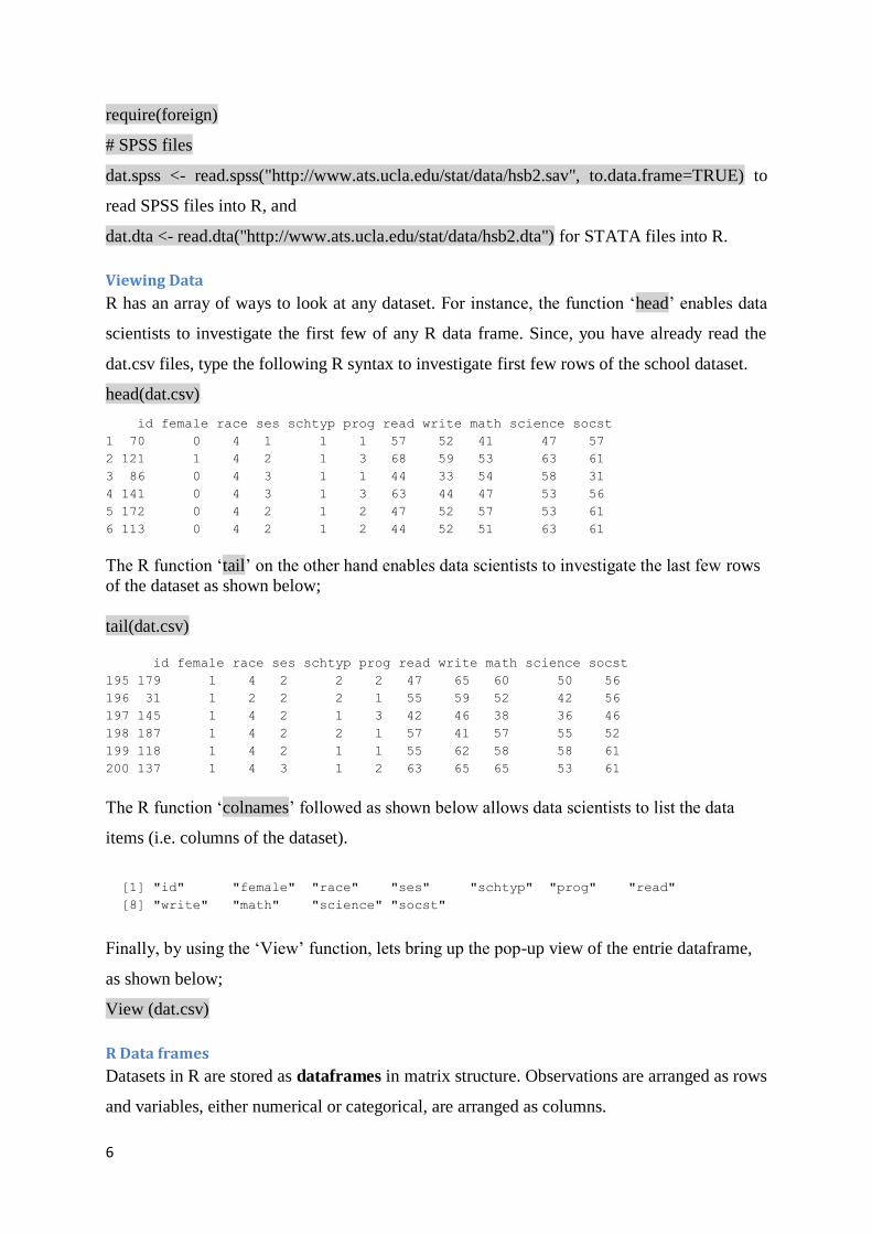
require(foreign)

# SPSS files

dat.spss <- read.spss("http://www.ats.ucla.edu/stat/data/hsb2.sav", to.data.frame=TRUE) to

read SPSS files into R, and

dat.dta <- read.dta("http://www.ats.ucla.edu/stat/data/hsb2.dta") for STATA files into R.

Viewing Data

R has an array of ways to look at any dataset. For instance, the function ‘head’ enables data

scientists to investigate the first few of any R data frame. Since, you have already read the

dat.csv files, type the following R syntax to investigate first few rows of the school dataset.

head(dat.csv)

id female race ses schtyp prog read write math science socst

1 70 0 4 1 1 1 57 52 41 47 57

2 121 1 4 2 1 3 68 59 53 63 61

3 86 0 4 3 1 1 44 33 54 58 31

4 141 0 4 3 1 3 63 44 47 53 56

5 172 0 4 2 1 2 47 52 57 53 61

6 113 0 4 2 1 2 44 52 51 63 61

The R function ‘tail’ on the other hand enables data scientists to investigate the last few rows

of the dataset as shown below;

tail(dat.csv)

id female race ses schtyp prog read write math science socst

195 179 1 4 2 2 2 47 65 60 50 56

196 31 1 2 2 2 1 55 59 52 42 56

197 145 1 4 2 1 3 42 46 38 36 46

198 187 1 4 2 2 1 57 41 57 55 52

199 118 1 4 2 1 1 55 62 58 58 61

200 137 1 4 3 1 2 63 65 65 53 61

The R function ‘colnames’ followed as shown below allows data scientists to list the data

items (i.e. columns of the dataset).

[1] "id" "female" "race" "ses" "schtyp" "prog" "read"

[8] "write" "math" "science" "socst"

Finally, by using the ‘View’ function, lets bring up the pop-up view of the entrie dataframe,

as shown below;

View (dat.csv)

R Data frames

Datasets in R are stored as dataframes in matrix structure. Observations are arranged as rows

and variables, either numerical or categorical, are arranged as columns.

7

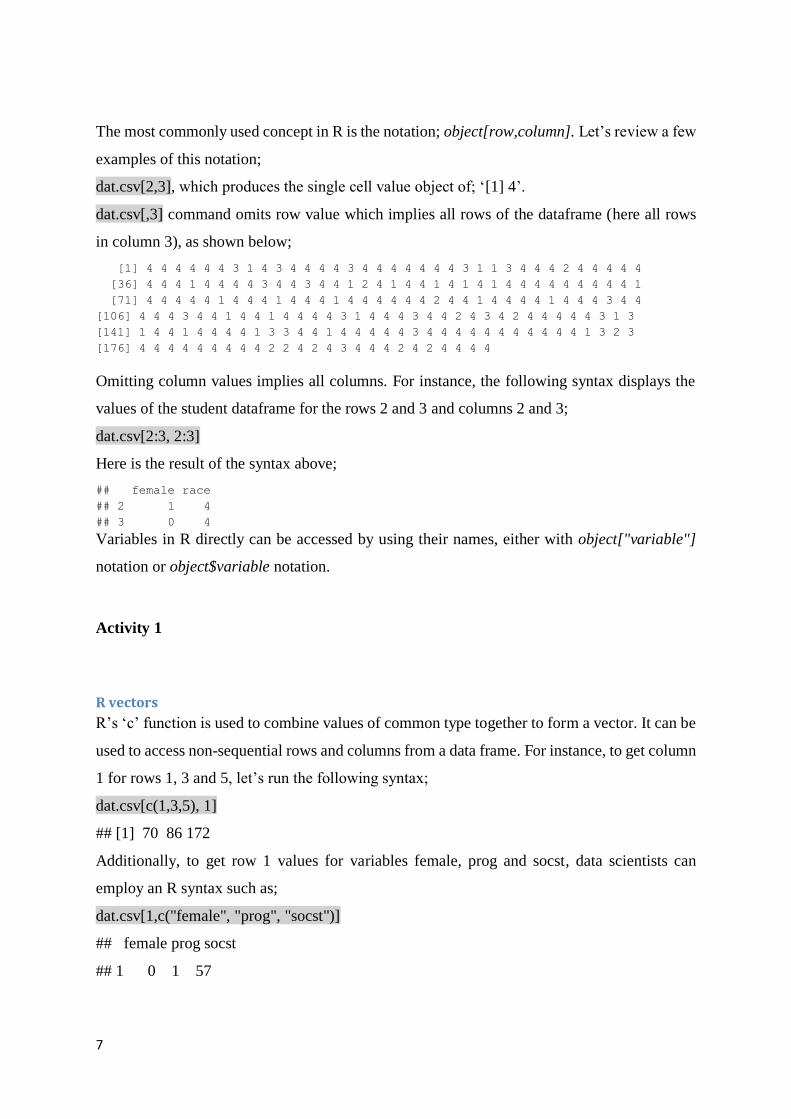
The most commonly used concept in R is the notation; object[row,column]. Let’s review a few

examples of this notation;

dat.csv[2,3], which produces the single cell value object of; ‘[1] 4’.

dat.csv[,3] command omits row value which implies all rows of the dataframe (here all rows

in column 3), as shown below;

[1] 4 4 4 4 4 4 3 1 4 3 4 4 4 4 3 4 4 4 4 4 4 4 3 1 1 3 4 4 4 2 4 4 4 4 4

[36] 4 4 4 1 4 4 4 4 3 4 4 3 4 4 1 2 4 1 4 4 1 4 1 4 1 4 4 4 4 4 4 4 4 4 1

[71] 4 4 4 4 4 1 4 4 4 1 4 4 4 1 4 4 4 4 4 4 2 4 4 1 4 4 4 4 1 4 4 4 3 4 4

[106] 4 4 4 3 4 4 1 4 4 1 4 4 4 4 3 1 4 4 4 3 4 4 2 4 3 4 2 4 4 4 4 4 3 1 3

[141] 1 4 4 1 4 4 4 4 1 3 3 4 4 1 4 4 4 4 4 3 4 4 4 4 4 4 4 4 4 4 4 1 3 2 3

[176] 4 4 4 4 4 4 4 4 4 2 2 4 2 4 3 4 4 4 2 4 2 4 4 4 4

Omitting column values implies all columns. For instance, the following syntax displays the

values of the student dataframe for the rows 2 and 3 and columns 2 and 3;

dat.csv[2:3, 2:3]

Here is the result of the syntax above;

## female race

## 2 1 4

## 3 0 4

Variables in R directly can be accessed by using their names, either with object["variable"]

notation or object$variable notation.

Activity 1

R vectors

R’s ‘c’ function is used to combine values of common type together to form a vector. It can be

used to access non-sequential rows and columns from a data frame. For instance, to get column

1 for rows 1, 3 and 5, let’s run the following syntax;

dat.csv[c(1,3,5), 1]

## [1] 70 86 172

Additionally, to get row 1 values for variables female, prog and socst, data scientists can

employ an R syntax such as;

dat.csv[1,c("female", "prog", "socst")]

## female prog socst

## 1 0 1 57

8

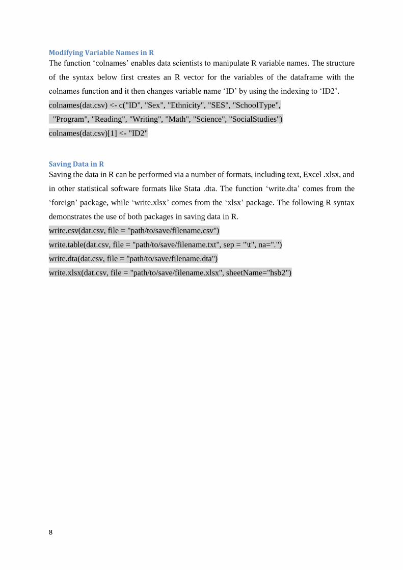
Modifying Variable Names in R

The function ‘colnames’ enables data scientists to manipulate R variable names. The structure

of the syntax below first creates an R vector for the variables of the dataframe with the

colnames function and it then changes variable name ‘ID’ by using the indexing to ‘ID2’.

colnames(dat.csv) <- c("ID", "Sex", "Ethnicity", "SES", "SchoolType",

"Program", "Reading", "Writing", "Math", "Science", "SocialStudies")

colnames(dat.csv)[1] <- "ID2"

Saving Data in R

Saving the data in R can be performed via a number of formats, including text, Excel .xlsx, and

in other statistical software formats like Stata .dta. The function ‘write.dta’ comes from the

‘foreign’ package, while ‘write.xlsx’ comes from the ‘xlsx’ package. The following R syntax

demonstrates the use of both packages in saving data in R.

write.csv(dat.csv, file = "path/to/save/filename.csv")

write.table(dat.csv, file = "path/to/save/filename.txt", sep = "\t", na=".")

write.dta(dat.csv, file = "path/to/save/filename.dta")

write.xlsx(dat.csv, file = "path/to/save/filename.xlsx", sheetName="hsb2")

9

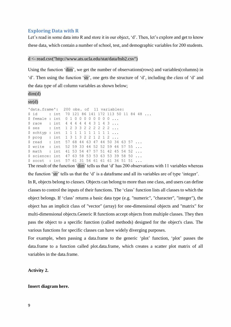
Exploring Data with R Let’s read in some data into R and store it in our object, ‘d’. Then, let’s explore and get to know

these data, which contain a number of school, test, and demographic variables for 200 students.

d <- read.csv("http://www.ats.ucla.edu/stat/data/hsb2.csv")

Using the function ‘dim’, we get the number of observations(rows) and variables(columns) in

‘d’. Then using the function ‘str’, one gets the structure of ‘d’, including the class of ‘d’ and

the data type of all column variables as shown below;

dim(d)

str(d)

'data.frame': 200 obs. of 11 variables:

$ id : int 70 121 86 141 172 113 50 11 84 48 ...

$ female : int 0 1 0 0 0 0 0 0 0 0 ...

$ race : int 4 4 4 4 4 4 3 1 4 3 ...

$ ses : int 1 2 3 3 2 2 2 2 2 2 ...

$ schtyp : int 1 1 1 1 1 1 1 1 1 1 ...

$ prog : int 1 3 1 3 2 2 1 2 1 2 ...

$ read : int 57 68 44 63 47 44 50 34 63 57 ...

$ write : int 52 59 33 44 52 52 59 46 57 55 ...

$ math : int 41 53 54 47 57 51 42 45 54 52 ...

$ science: int 47 63 58 53 53 63 53 39 58 50 ...

$ socst : int 57 61 31 56 61 61 61 36 51 51 ...

The result of the function ‘dim’ tells us that ‘d’ has 200 observations with 11 variables whereas

the function ‘str’ tells us that the ‘d’ is a dataframe and all its variables are of type ‘integer’.

In R, objects belong to classes. Objects can belong to more than one class, and users can define

classes to control the inputs of their functions. The ‘class’ function lists all classes to which the

object belongs. If ‘class’ returns a basic data type (e.g. "numeric", "character", "integer"), the

object has an implicit class of "vector" (array) for one-dimensional objects and "matrix" for

multi-dimensional objects.Generic R functions accept objects from multiple classes. They then

pass the object to a specific function (called methods) designed for the object's class. The

various functions for specific classes can have widely diverging purposes.

For example, when passing a data.frame to the generic ‘plot’ function, ‘plot’ passes the

data.frame to a function called plot.data.frame, which creates a scatter plot matrix of all

variables in the data.frame.

Activity 2.

Insert diagram here.

10

Data Wrangling with R R package ‘dplyr’ is a widely used package to modify data. The package has five main

functions which we will be using each of these functions later in the unit in detail.

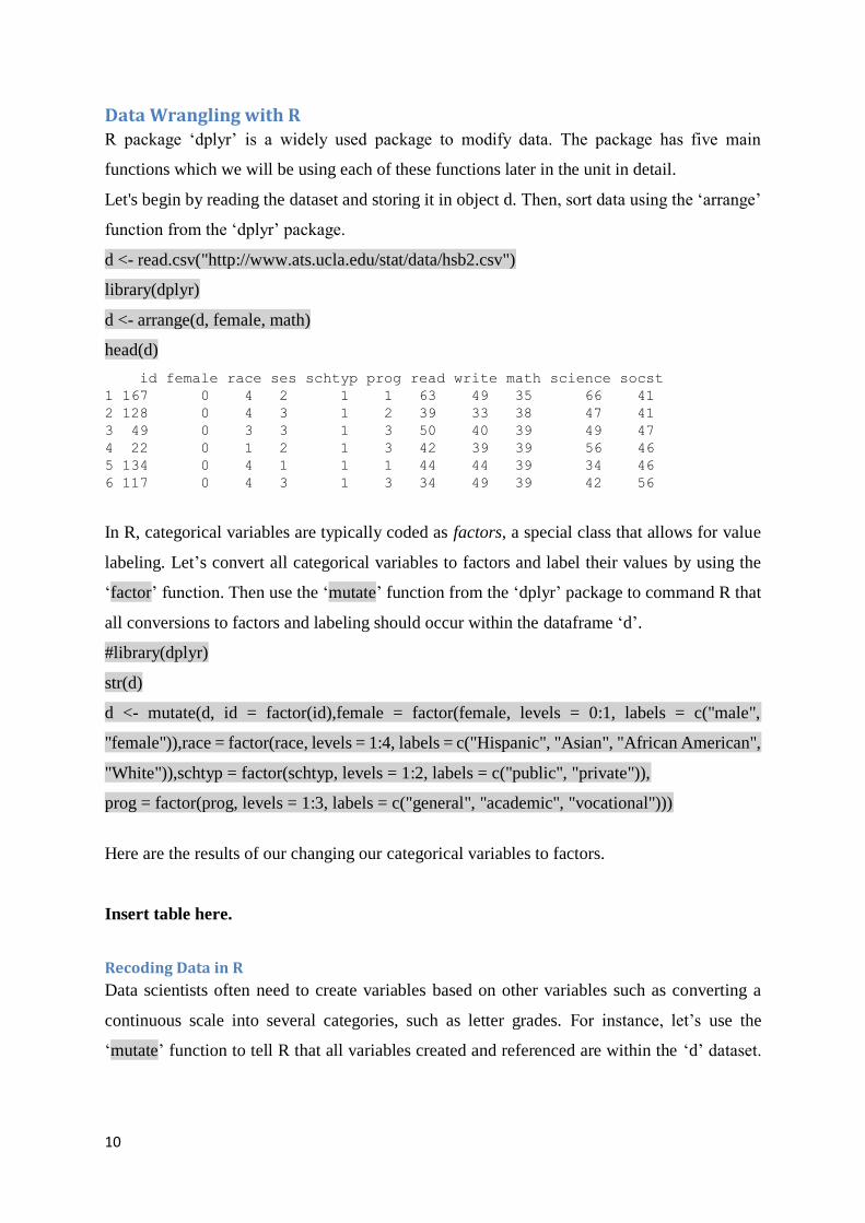
Let's begin by reading the dataset and storing it in object d. Then, sort data using the ‘arrange’

function from the ‘dplyr’ package.

d <- read.csv("http://www.ats.ucla.edu/stat/data/hsb2.csv")

library(dplyr)

d <- arrange(d, female, math)

head(d)

id female race ses schtyp prog read write math science socst

1 167 0 4 2 1 1 63 49 35 66 41

2 128 0 4 3 1 2 39 33 38 47 41

3 49 0 3 3 1 3 50 40 39 49 47

4 22 0 1 2 1 3 42 39 39 56 46

5 134 0 4 1 1 1 44 44 39 34 46

6 117 0 4 3 1 3 34 49 39 42 56

In R, categorical variables are typically coded as factors, a special class that allows for value

labeling. Let’s convert all categorical variables to factors and label their values by using the

‘factor’ function. Then use the ‘mutate’ function from the ‘dplyr’ package to command R that

all conversions to factors and labeling should occur within the dataframe ‘d’.

#library(dplyr)

str(d)

d <- mutate(d, id = factor(id),female = factor(female, levels = 0:1, labels = c("male",

"female")),race = factor(race, levels = 1:4, labels = c("Hispanic", "Asian", "African American",

"White")),schtyp = factor(schtyp, levels = 1:2, labels = c("public", "private")),

prog = factor(prog, levels = 1:3, labels = c("general", "academic", "vocational")))

Here are the results of our changing our categorical variables to factors.

Insert table here.

Recoding Data in R

Data scientists often need to create variables based on other variables such as converting a

continuous scale into several categories, such as letter grades. For instance, let’s use the

‘mutate’ function to tell R that all variables created and referenced are within the ‘d’ dataset.

11

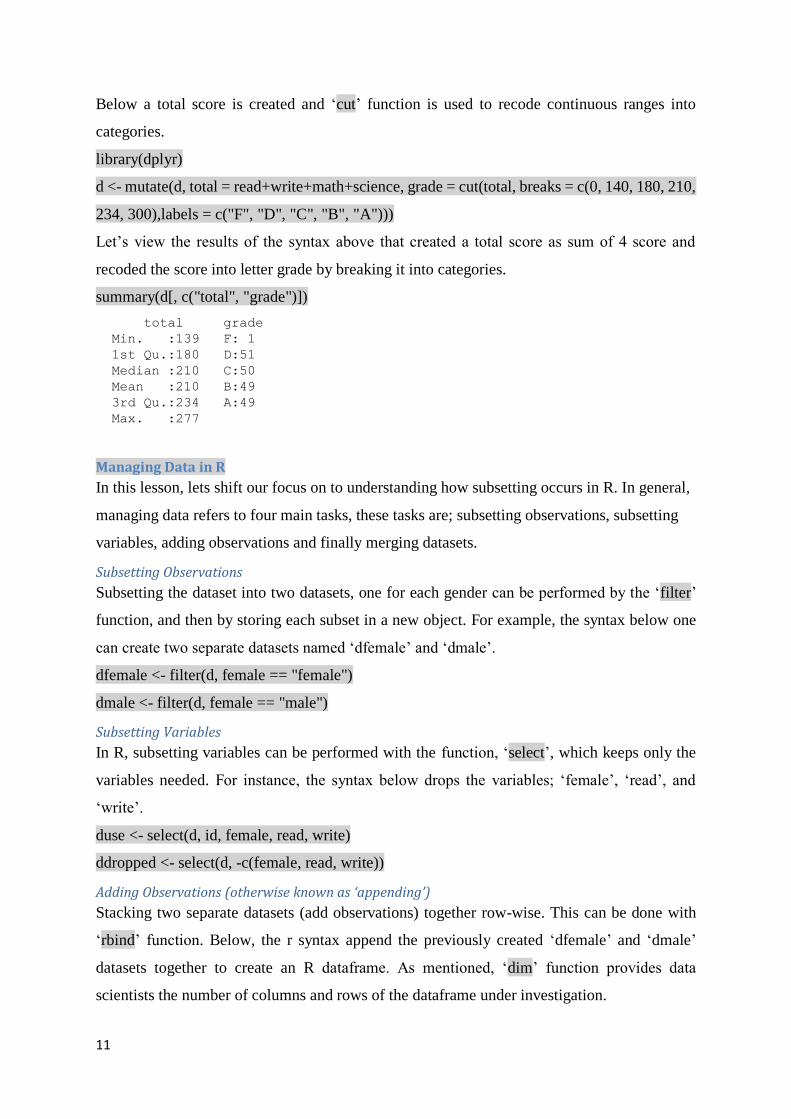
Below a total score is created and ‘cut’ function is used to recode continuous ranges into

categories.

library(dplyr)

d <- mutate(d, total = read+write+math+science, grade = cut(total, breaks = c(0, 140, 180, 210,

234, 300),labels = c("F", "D", "C", "B", "A")))

Let’s view the results of the syntax above that created a total score as sum of 4 score and

recoded the score into letter grade by breaking it into categories.

summary(d[, c("total", "grade")])

total grade

Min. :139 F: 1

1st Qu.:180 D:51

Median :210 C:50

Mean :210 B:49

3rd Qu.:234 A:49

Max. :277

Managing Data in R

In this lesson, lets shift our focus on to understanding how subsetting occurs in R. In general,

managing data refers to four main tasks, these tasks are; subsetting observations, subsetting

variables, adding observations and finally merging datasets.

Subsetting Observations

Subsetting the dataset into two datasets, one for each gender can be performed by the ‘filter’

function, and then by storing each subset in a new object. For example, the syntax below one

can create two separate datasets named ‘dfemale’ and ‘dmale’.

dfemale <- filter(d, female == "female")

dmale <- filter(d, female == "male")

Subsetting Variables

In R, subsetting variables can be performed with the function, ‘select’, which keeps only the

variables needed. For instance, the syntax below drops the variables; ‘female’, ‘read’, and

‘write’.

duse <- select(d, id, female, read, write)

ddropped <- select(d, -c(female, read, write))

Adding Observations (otherwise known as ‘appending’)

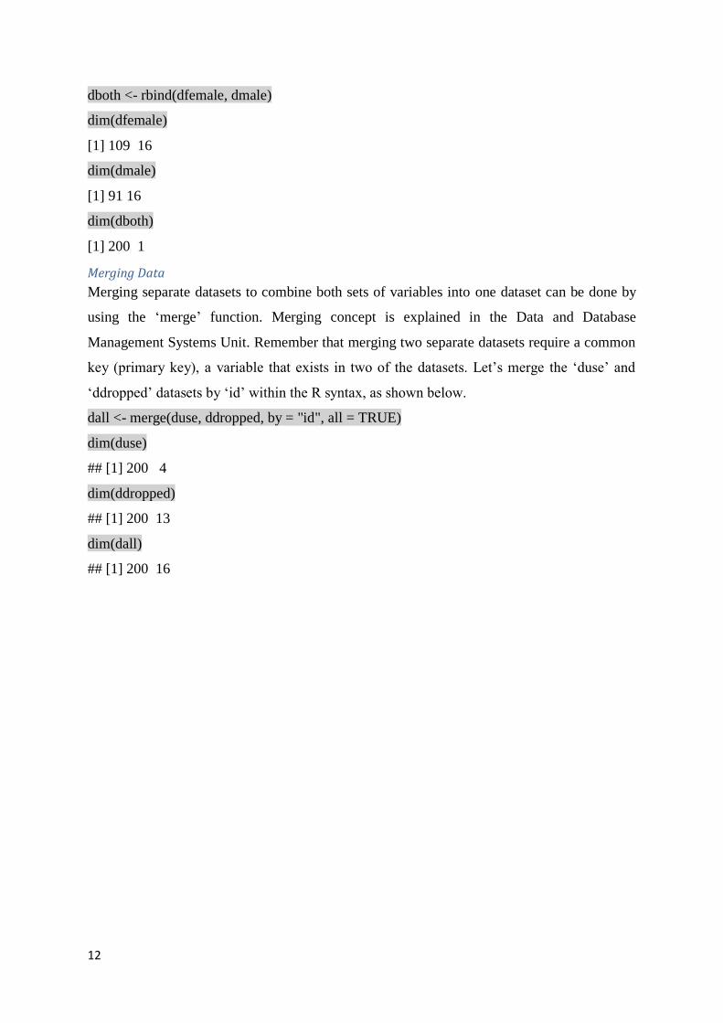
Stacking two separate datasets (add observations) together row-wise. This can be done with

‘rbind’ function. Below, the r syntax append the previously created ‘dfemale’ and ‘dmale’

datasets together to create an R dataframe. As mentioned, ‘dim’ function provides data

scientists the number of columns and rows of the dataframe under investigation.

12

dboth <- rbind(dfemale, dmale)

dim(dfemale)

[1] 109 16

dim(dmale)

[1] 91 16

dim(dboth)

[1] 200 1

Merging Data

Merging separate datasets to combine both sets of variables into one dataset can be done by

using the ‘merge’ function. Merging concept is explained in the Data and Database

Management Systems Unit. Remember that merging two separate datasets require a common

key (primary key), a variable that exists in two of the datasets. Let’s merge the ‘duse’ and

‘ddropped’ datasets by ‘id’ within the R syntax, as shown below.

dall <- merge(duse, ddropped, by = "id", all = TRUE)

dim(duse)

## [1] 200 4

dim(ddropped)

## [1] 200 13

dim(dall)

## [1] 200 16

13

Introduction to Data Wrangling with R Data scientists often must deal with untidy or incomplete data. The raw data obtained from

different data sources is often unusable at the beginning of every data science project. The

activity that data scientists perform on the raw data to make it usable to input to statistical

modelling and machine learning algorithms is called data wrangling or data munging.

Similarly, to create an efficient ETL (extract, transform and load) pipeline or create data

visualizations, data scientists should be prepared to do a lot of data wrangling.

Data wrangling is a process of data manipulation and transformation that enables analysis. In

other words, it is the process of manually converting or mapping data from one raw form into

another format that allows for more convenient consumption of the data with the help of semi-

automated tools.

Data wrangling is an important part of any data science project. By dropping null values,

filtering, and selecting the right data, and working with time series, you can ensure that any

machine learning or treatment you apply to your cleaned-up data is fully effective.

It is important to remember three steps goals of data wrangling when working with data. These

are;

1. Figure out what you need to do,

2. Describe those tasks in the form of a computer program (i.e. R),

3. Execute the program.

Data Wrangling with R ‘dplyr’ package

Remember that the ‘dplyr’ package makes the steps involved in data wrangling effective by; it

helps data scientists think about data manipulation challenges, it provides simple functions that

correspond to the most common data manipulation tasks and it uses efficient backends, so data

scientists spend less time waiting for the processing power of the computers.This section

introduces dplyr’s basic set of tools, and shows how to apply them to data frames.

In data wrangling, there a few tasks that any data science project needs to deal with. Some of

these tasks are;

• Filtering rows in data,,

• Selecting columns of data

• Adding new variables in data,

• Sorting data, and

• Aggregating data.

14

In introduction to R, we have explored some of these tasks with R. In this section, we will

explore these tasks and others with a powerful R package, ‘dplyr’ package. The package,

‘dplyr’ gives data scientists tools to do these tasks, and it does so in a way that streamlines the

analytics workflow. It may be said that ‘dplyr’ is almost perfectly suited to data science work,

as it is performed.

As mentioned earlier in the unit, the package ‘dplyr’ has five main commands. These

commands are; filter, select, mutate, arrange, and summarize. Below, we will explore each of

the steps in greater detail.

1. Filter ()

The function ‘filter’ subsets data by keeping rows that meet specified conditions. An example

of the function is provided below.

library(dplyr)

library(ggplot2)

head(diamonds)

df.diamonds_ideal <- filter(diamonds, cut=="Ideal")

In this example, sub-setting (i.e., filtering) the diamonds dataset and keeping only the rows

where cut==Ideal is performed.

2. Select ()

The function ‘select’ enables users to select specific columns of the data. In the following

example, lets inspect the df.diamonds_ideal dataframe to see the components of it. Then, we

will modify the data frame by selecting the columns desired. Lets examine the data first with

the following R syntax;

head(df.diamonds_ideal)

carat cut color clarity depth table price x y z

0.23 Ideal E SI2 61.5 55 326 3.95 3.98 2.43

0.23 Ideal J VS1 62.8 56 340 3.93 3.90 2.46

0.31 Ideal J SI2 62.2 54 344 4.35 4.37 2.71

0.30 Ideal I SI2 62.0 54 348 4.31 4.34 2.68

0.33 Ideal I SI2 61.8 55 403 4.49 4.51 2.78

0.33 Ideal I SI2 61.2 56 403 4.49 4.50 2.75

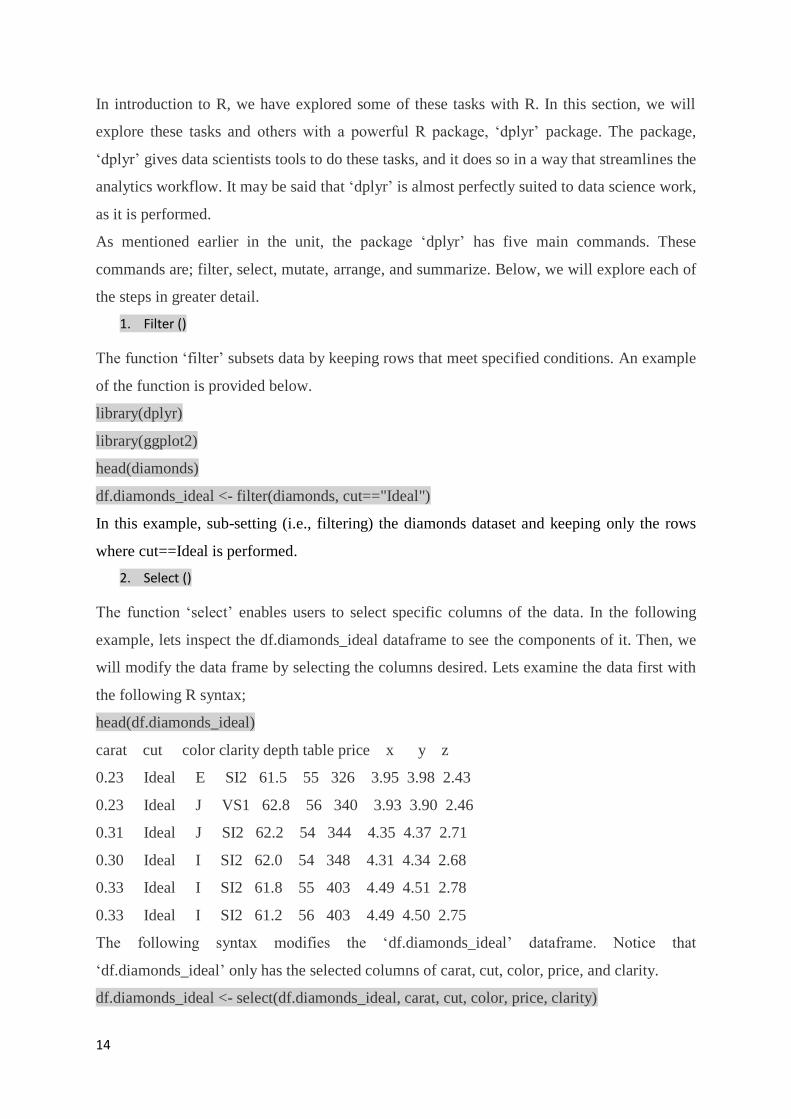
The following syntax modifies the ‘df.diamonds_ideal’ dataframe. Notice that

‘df.diamonds_ideal’ only has the selected columns of carat, cut, color, price, and clarity.

df.diamonds_ideal <- select(df.diamonds_ideal, carat, cut, color, price, clarity)

15

head(df.diamonds_ideal)

carat cut color price clarity

0.23 Ideal E 326 SI2

0.23 Ideal J 340 VS1

0.31 Ideal J 344 SI2

0.30 Ideal I 348 SI2

0.33 Ideal I 403 SI2

0.33 Ideal I 403 SI2

3. Mutate ()

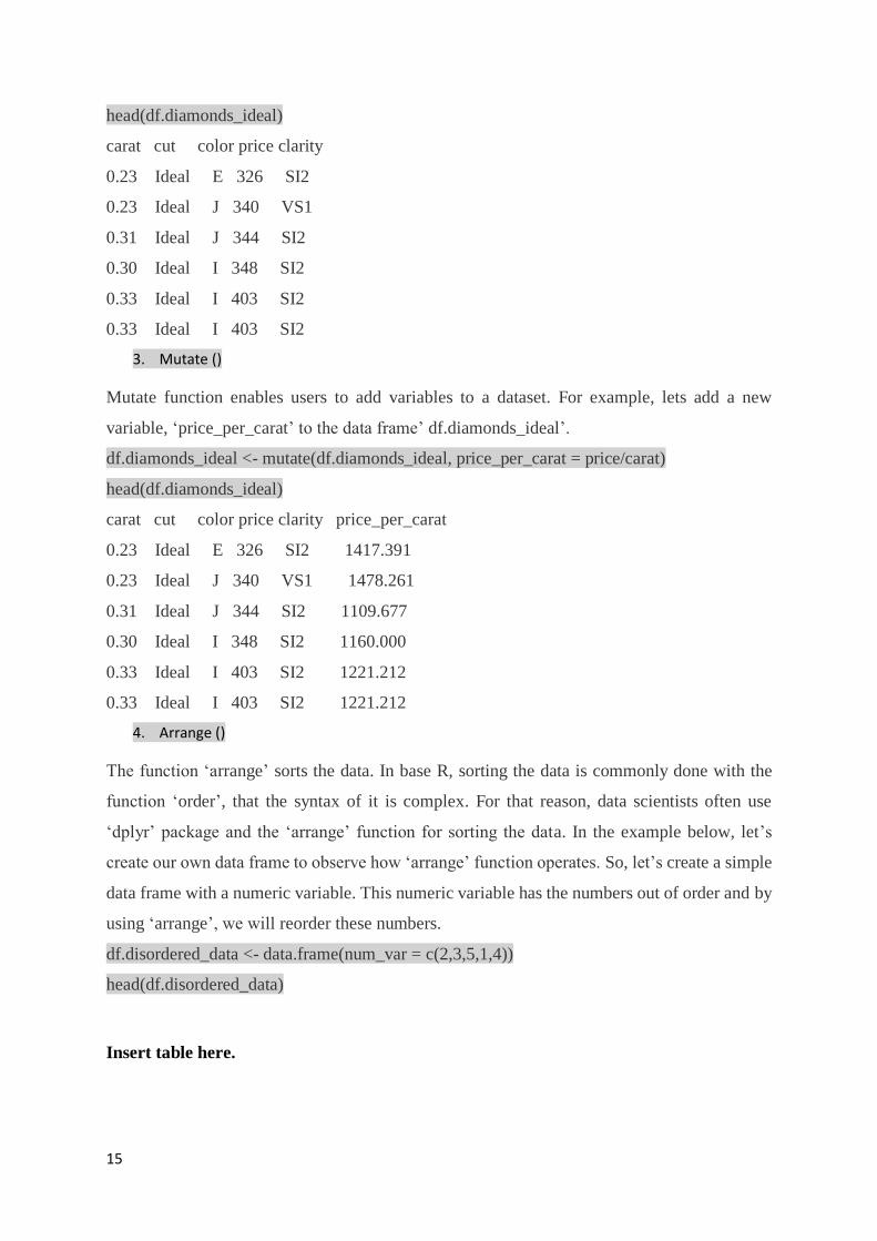
Mutate function enables users to add variables to a dataset. For example, lets add a new

variable, ‘price_per_carat’ to the data frame’ df.diamonds_ideal’.

df.diamonds_ideal <- mutate(df.diamonds_ideal, price_per_carat = price/carat)

head(df.diamonds_ideal)

carat cut color price clarity price_per_carat

0.23 Ideal E 326 SI2 1417.391

0.23 Ideal J 340 VS1 1478.261

0.31 Ideal J 344 SI2 1109.677

0.30 Ideal I 348 SI2 1160.000

0.33 Ideal I 403 SI2 1221.212

0.33 Ideal I 403 SI2 1221.212

4. Arrange ()

The function ‘arrange’ sorts the data. In base R, sorting the data is commonly done with the

function ‘order’, that the syntax of it is complex. For that reason, data scientists often use

‘dplyr’ package and the ‘arrange’ function for sorting the data. In the example below, let’s

create our own data frame to observe how ‘arrange’ function operates. So, let’s create a simple

data frame with a numeric variable. This numeric variable has the numbers out of order and by

using ‘arrange’, we will reorder these numbers.

df.disordered_data <- data.frame(num_var = c(2,3,5,1,4))

head(df.disordered_data)

Insert table here.

16

The syntax, arrange (df.disordered_data, num_var), orders the data points of the dataframe

whilst the syntax arrange(df.disordered_data, desc(num_var)) sorts the data in descending

order.

5. Summarize ()

The function ‘summarize’ is a very useful function which enables data scientists to compute

summary statistics of the data. Having a look at the summary statistics of the data allows data

scientists to understand the distributional features of the data which we will explore further in

the unit data exploration and visualisation.

summarize(df.diamonds_ideal, avg_price = mean(price, na.rm = TRUE) )

avg_price

3457.542

As you have noticed that the syntax and function of all these verbs are very similar.

• The first argument is always a data frame,

• The subsequent arguments describe what to do with the data frame. You can refer to

columns in the data frame directly without using $, and

• The result is always a new data frame.

Together these properties make it easy to chain together (merge) multiple simple steps to

achieve a complex result. These five functions provide basis of a language of data manipulation

with ‘dplyr’. In summary, data scientists alter an untidy or incomplete data frame in five useful

ways;

1. Reorder the rows by the function (arrange()),

2. Pick observations and variables of interest by the function filter() and,

3. Pick observations and variables of interest by the function select()),

4. Add new variables that are functions of existing variables by the function (mutate())

and finally,

5. Collapse many values to a summary by the function (summarise()).

Activity 3.

Chaining in ‘dplyr’ Moving beyond the examples above, the real power of the ‘dplyr’ package comes when data

scientists chain different commands together (or, chain different ‘dplyr’ commands together

with commands and functions from other packages).

17

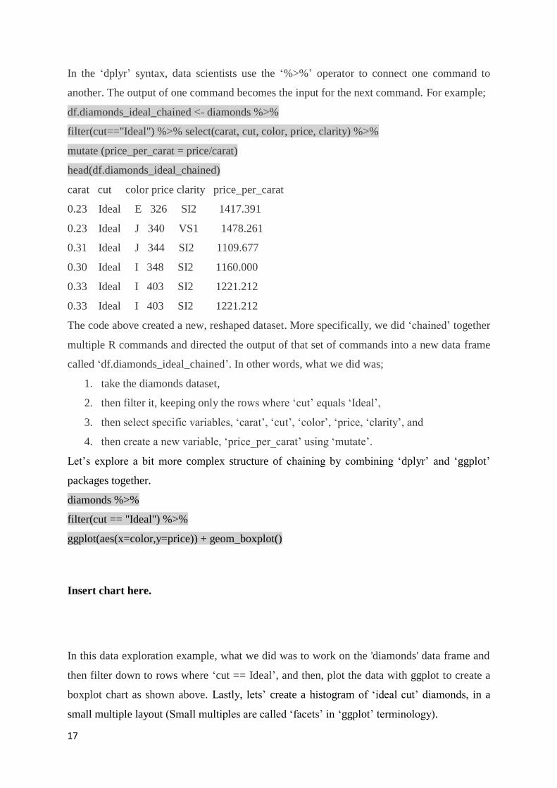
In the ‘dplyr’ syntax, data scientists use the ‘%>%’ operator to connect one command to

another. The output of one command becomes the input for the next command. For example;

df.diamonds_ideal_chained <- diamonds %>%

filter(cut=="Ideal") %>% select(carat, cut, color, price, clarity) %>%

mutate (price_per_carat = price/carat)

head(df.diamonds_ideal_chained)

carat cut color price clarity price_per_carat

0.23 Ideal E 326 SI2 1417.391

0.23 Ideal J 340 VS1 1478.261

0.31 Ideal J 344 SI2 1109.677

0.30 Ideal I 348 SI2 1160.000

0.33 Ideal I 403 SI2 1221.212

0.33 Ideal I 403 SI2 1221.212

The code above created a new, reshaped dataset. More specifically, we did ‘chained’ together

multiple R commands and directed the output of that set of commands into a new data frame

called ‘df.diamonds_ideal_chained’. In other words, what we did was;

1. take the diamonds dataset,

2. then filter it, keeping only the rows where ‘cut’ equals ‘Ideal’,

3. then select specific variables, ‘carat’, ‘cut’, ‘color’, ‘price, ‘clarity’, and

4. then create a new variable, ‘price_per_carat’ using ‘mutate’.

Let’s explore a bit more complex structure of chaining by combining ‘dplyr’ and ‘ggplot’

packages together.

diamonds %>%

filter(cut == "Ideal") %>%

ggplot(aes(x=color,y=price)) + geom_boxplot()

Insert chart here.

In this data exploration example, what we did was to work on the 'diamonds' data frame and

then filter down to rows where ‘cut == Ideal’, and then, plot the data with ggplot to create a

boxplot chart as shown above. Lastly, lets’ create a histogram of ‘ideal cut’ diamonds, in a

small multiple layout (Small multiples are called ‘facets’ in ‘ggplot’ terminology).

18

diamonds %>%

filter(cut == "Ideal") %>%

ggplot(aes(price)) + geom_histogram() + facet_wrap(~ color)

Insert table here.

Four crucial data wrangling tasks with R

There is an array of data wrangling tasks in any dataset in practise. Each dataset is unique which

requires customised data wrangling tasks to be thought through and implemented. This is due

to the fat that each data generation process involves, collects and generates data that given the

business goals need to be dealt with at the data wrangling stage. Having said that, there are four

widely used data wrangling tasks that are in the toolset of data scientists. These are;

1. Adding a column to an existing dataframe,

2. Getting data summaries by subgrouping,

3. Sorting the results, and

4. Reshaping the dataframe.

Before going into detail for each of these main data wrangling tasks by using R, let’s create a

hypothetical data frame by entering values into R. Then, store this dataset as ‘CompanyData’.

fy <- c(2010,2011,2012,2010,2011,2012,2010,2011,2012)

company <- c("Apple","Apple","Apple","Google","Google","Google","Microsoft","Microsoft","Microsoft")

revenue <- c(65225,108249,156508,29321,37905,50175,62484,69943,73723)

profit <- c(14013,25922,41733,8505,9737,10737,18760,23150,16978)

CompanyData <- data.frame(fy, company, revenue, profit)

R code above will create a data frame displayed below, stored in a variable named

‘CompanyData’:

Insert table here.

To analyse structure of the data frame created, data scientists use the ‘str’ function to see that

the year is being treated as a number and not as a year or factor;

str(CompanyData)

'data.frame': 9 obs. of 4 variables:

$ fy : num 2010 2011 2012 2010 2011 ...

$ company: Factor w/ 3 levels "Apple","Google",..: 1 1 1 2 2 2 3 3 3

19

$ revenue: num 65225 108249 156508 29321 37905 ...

$ profit : num 14013 25922 41733 8505 9737 ...

As is seen, the dataframe has 9 observations and 4 variables. The variable ‘fy’ has numeric

data, which in fact represents the ‘year’ (essentially a date field). In R, date fields need to be

represented as factors though. The variables ‘company’ is a factor variable with three levels

(Apple, Google, and Microsoft), whereas the variables of ‘revenue’, and ‘profit’ are numeric

variables. To perform group by analyses by year, one can change the ‘fy’ column of numbers

into a column that contains R categories (i.e. factors) with the following command;

CompanyData$fy <- factor(CompanyData$fy, ordered = TRUE)

This process converts the numeric variable ‘year’ into a factor format which represents the

nature of this data to more effectively stored and displayed in the dataframe.

1. Adding an additional column to an existing data frame

Adding a new column to a data frame is a commonly applied method in data science. R allows

adding a new column to a data frame based on one or more other columns in several ways.

1.1 To create a new column that is the sum of two existing columns

dataFrame$newColumn <- dataFrame$oldColumn1 + dataFrame$oldColumn2

This syntax structure creates a new column called ‘newColumn’ with the sum of

o’ldColumn1’+‘oldColumn2’ in each row. Let’s add a column for ‘profit margin’ in our sample

dataframe by dividing profit by revenue and then multiplying by 100.

CompanyData$margin <- (companiesData$profit / CompanyData$revenue) * 100

R syntax above results in the dataset as shown below;

Insert table here.

R allows data scientists to use many ways to achieve the same business goal. For instance,

using the function ‘transform’, a new column called ‘margin’ that is a function of the revenue

and profit can be generated. The syntax for this is; dataFrame <- transform (dataFrame,

newColumn = oldColumn1 + oldColumn2) and the application to our sample dataframe would

be as;

CompanyData <- transform (CompanyData, margin = (profit/revenue) * 100)

Additionally, use the ‘round’ function to round the column results to one decimal place. As

shown;

20

CompanyData <- transform (CompanyData, margin = round((profit/revenue) * 100, 1))

1.2 Using functions

Similarly, R’s ‘mapply’ function and ‘mutate’ functions (as we explored earlier in the unit) do

achiev the same outcomes in adding a new column to the dataframe. The structure

dataFrame$newColumn<-mapply(someFunction,dataFrame$column1, dataFrame$column2,

dataFrame$column3) applies the function ‘someFunction()’ to the data in column1, column2

and column3 of each row of the data frame. One advantage ‘mapply’ has over ‘transform’

though is that data scientists can use columns from different data frames.

CompanyData$margin<-mapply(profitMargin,CompanyData$profit, CompanyData$revenue)

CompanyData <- mutate (CompanyData, margin = round((profit/revenue) * 100, 1))

2. Getting summaries by subgrouping

R’s ‘plyr’ package enables data scientists splitting up the dataset by one or more factors, apply

some function, then combine the results back into a dataframe. The function ‘ddply’ of the

‘plyr’ package performs a "split-apply-combine" concept on a dataframe and then produces a

new separate data frame with the results. The format for splitting a dataframe by multiple

factors and applying the function ‘ddply’ is as;

ddply (mydata, c('column name of a factor to group by', 'column name of the second factor to

group by'), summarize or transform, newcolumn = myfunction(column name(s) I want the

function to act upon))

Let's take a more detailed look at this syntax. The ddply() function’s first argument is the name

of the original data frame and the second argument is the name of the column or columns to

subset the dataframe by. The third commands ddply() function whether to return just the

resulting data points (summarize) or the entire data frame with a new column giving the desired

data point per factor in every row. Finally, the fourth argument names the new column and then

lists the function desired by ddply() to use.

For example, to get the highest profit margins for each company, let’s split the data frame by

a factor, ‘company’. Then, to get the highest value and company name for each company, use

‘summarize’ as the third argument as shown below;

highestProfitMargins<ddply(CompanyData,(company),summarize,bestMargin=max(margin))

Insert table here.

21

Remember, ‘ddply’ can apply more than one function at a time, for example;

myResults<ddply(CompanyData,'company',transform,highestMargin=max(margin),lowestM

argin=min(margin))

Insert table here.

While ‘ddply’ designed for “split-apply-combine” concept, in other words applying it to

different categories of the data, data scientists can still use it to apply a function to entire data

frame at once.

3. Sorting data

R enables data scientists to sort the dataframe in an array of ways with the function ‘order’.

This function allows data scientists to have the sorting they prefer with a simple sort by one

column. For instance, companyOrder <- order(CompanyData$margin) just achieves that.

Let’s run the following R syntax to observe how R enables data scientists to sort the

dataframe with different approaches.

companiesOrdered <- CompanyData[companyOrder,]

companiesOrdered <- CompanyData[order(CompanyData$margin),]

companiesOrdered <- CompanyData[order(CompanyData$margin),c("fy", "company")]

companyOrder <- order(-CompanyData$margin)

companiesOrdered <- CompanyData[companyOrder,]

companiesOrdered <- CompanyData[with(CompanyData, order(fy, -margin)),]

4. Reshaping data

One of the most important concepts in R that data scientists should always remember is that

different analysis tools (packages) in R require the data in specific formats. Therefore, one of

the most common tasks in R data manipulation involving advance data science projects is

switching between "wide" and "long" data formats. For example, it is usually easier to visualize

data using the popular ‘ggplot2’ graphing package if the dataframe is in long format.

Long format has one measurement per row and most likely multiple categories, such as;

Insert table here.

22

Wide format on the other hand means that the dataframe has multiple measurement columns

across each row, such as;

Insert table here.

Let’s use R’s ‘reshape2’ package and its ‘melt’ function to reshape dataframes, in particulalry

reshape dataframes that are wide format into long format. The function ‘melt’ uses the

following format to assign results to a variable named ‘longData’; longData <- melt (original

data frame, a vector of your category variables).

Using the data frame of our sample data, wide-to-long reshaping of the dataframe can simply

be achieved by;

companiesLong <- melt (companiesData, c("fy", "company"))

Insert table here.

Once the data frame is treated with the function ‘melted’, it can then be “cast” into any shape.

The function ‘dcast’ takes a long format data frame as input and enables data scientists to

create a wide format dataframe. The format of the

wideDataFrame<-dcast(longDataFrame,idVariableColumn1+idVariableColumn2~

variableColumn,value.var="Name of column with the measurement values"). As seen, the

function ‘dcast’ takes the name of a long data frame as the first argument.

Using the data frame of our sample data, long-to-wide reshaping of the dataframe can simply

be achieved by;

companiesWide<-

dcast(companiesLong,fy+company~financialCategory,value.var="amount")

Data Imputation with R Data imputation means assigning sensible and rational values to incomplete rows in each

dataset, which is a function of a known data generation process. In statistical modelling and

machine learning, all available techniques require data to be without missing values. Therefore,

23

data scientists face the dilemma of whether to use of only those rows with complete information

or impute in a plausible value for the missing observations.

For instance, the values of the gender in the rows 13 to 18 have missing data in the following

dataset. There are also other missing vakus in this dataset. Some rows of the

annocuecementsView and ParentAnsweringSurvey variables also have some missing values.

These missing values is the fucnon of the data generation process, such as, data entry errors or

incomplete answers to ghe questionerie.

Insert diagram here.

Missing completely at random (MCAR) describes data where the complete cases are a

random sample of the originally identified set of cases. Since the complete cases are

representative of the originally identified sample, inferences based on only the complete

cases are applicable to the larger sample and the target population. Missing at random

(MAR) to describe data that are missing for reasons related to completely observed variables

in the data set (Rubin, 1976).

In this lesson, we will learn how to apply multiple imputation models (commonly applied

imputation technique by data scientist in the industry) by using R. There are several imputation

packages in R. However, we will be using the package ‘Amelia’ to master the imputation of

datasets with incomplete data.

There are two versions of Amelia in R. First, Amelia II exists as a package for the R statistical

software package. Data scientists can utilize their knowledge of the R language to run Amelia

II at the command line or to create scripts that will run Amelia II and preserve the commands

for future use. Alternatively, data scientists can use AmeliaView, where an interactive

Graphical User Interface (GUI) enables setting options and run Amelia package without any

knowledge of the R programming language. We will be practising with AmeliaView.

AmeliaView Menu Guide

Below is a guide to the AmeliaView menus with references back to the users's guide. The same

principles from the user's guide apply to AmeliaView. The only difference is how you interact

with the program. Whether you use the GUI or the command line versions, the same underlying

code is being called, and so you can read the command line-oriented discussion above even if

you intend to use the GUI.

24

Loading AmeliaView

The way to load AmeliaView is to open an R session and type the following two commands:

library(Amelia)

AmeliaView()

This will bring up the AmeliaView window on any platform. On the Windows operating

system, there is an alternative way to start AmeliaView from the Desktop. Once installed, there

should be a desktop icon for AmeliaView. Simply double-click this icon and the AmeliaView

window should appear. If, for some reason, this approach does not work, simply open an R

session, and use the approach above.

Insert screenshot here.

Loading a data set into AmeliaView

AmeliaView load with a welcome screen that has buttons which can load a data in many of the

common formats. Each of these will bring up a window for choosing your dataset. Note that

these buttons are only a subset of the possible ways to load data in AmeliaView. Under the File

menu, you will find more options, including the datasets included in the package (africa and

freetrade). You will also find import commands for Comma-Separated Values (.CSV), Tab-

Delimited Text (.TXT), Stata v.5-10 (. DTA), SPSS (.DAT), and SAS Transport (. XPORT).

Note that when using a CSV file, AmeliaView assumes that your file has a header.

Insert screenshot here.

Variable dashboard

Once a dataset is loaded, AmeliaView will show the variable dashboard.

In this mode, you will see a table of variables, with the current options for each of them shown,

along with a few summary statistics. You can reorder this table by any of these columns by

clicking on the column headings. This might be helpful to, say, order the variables by mean or

amount of missingness.

Insert screenshot here.

25

You can set options for individual variables by the right-click context menu or through the

Variables menu. For instance, clicking \Set as Time-Series Variable" will set the currently

selected variable in the dashboard as the time-series variable. Certain options are disabled until

other options are enabled. For instance, you cannot add a lagged variable to the imputation

until you have set the time-series variable. Note that any factor in the data is marked as a ID

variable by default, since a factor cannot be included in the imputation without being set as an

ID variable, a nominal variable, or the cross-section variable. If there is a factor that fails to

meet one of these conditions, a red ag will appear next to the variable name. Here are some of

the commonly used functionalities in AmeliaView:

• Set as Time-Series Variable - Sets the currently selected variable to the time-series

variable. The time-series variable will have a clock icon next to it.

• Set as Cross-Section Variable - Sets the currently selected variable to the cross-section

variable. The cross-section variable will have a person icon next to it.

• Unset as Time-Series Variable - Removes the time-series status of the variable.

• Unset as Cross-Section Variable - Removes the cross-section status of the variable.

• Add Lag/Lead - Adds versions of the selected variables either lagged back (\lag") or

forward(\lead").

• Remove Lag/Lead - Removes any lags or leads on the selected variables.

• Plot Histogram of Selected - Plots a histogram of the selected variables. This command

will attempt to put all of the histograms on one page, but if more than nine histograms

are requested, they will appear on multiple pages.

• Add Transformation. - Adds a transformation setting for the selected variables. Note

that each variable can only have one transformation and the time-series and cross-

section variables cannot be transformed.

• Remove Transformation - Removes any transformation for the selected variables.

• Add or Edit Bounds - Opens a dialog box to set logical bounds for the selected variable.

The Variable menu and the variable dashboard are the place to set variable-level options, but

global options are set in the Options menu. Under the global options menu, data scientists can

have advance settings of the AmeliaView changed. In this lesson, we will not be exploring

these advance options.

26

Imputing and checking diagnostics

Once data scientists have set all the relevant options in AmeliaView, they then can impute data

by clicking the ‘Impute!’ button in the toolbar. Once the imputations are complete, “Successful

Imputation!" message appears at the bottom bar. By clicking on this message data scientists

can open the folder containing the imputed datasets and explore the results.

If there was an error during the imputation, the output log will pop-up and provides the error

message along with some information about how to fix the problem. Once the problem is fixed

simply click “Impute!" again. to understand how AmeliaView ran, simply click the “Show

Output Log" button. The log also shows the call to the ‘amelia’ function in R.

Insert chart here.

Upon the successful completion of an imputation, the diagnostics menu will become available.

• Compare Plots - This will display the relative densities of the observed (red) and

imputed (black) data. The density of the imputed values are the average You will have

to replace the x argument in the amelia call to the name of you dataset in the R session.

imputations across all of the imputed datasets.

Insert screenshot here.

• Overimpute - This will run Amelia on the full data with one cell of the chosen variable

artificially set to missing and then check the result of that imputation against the truth.

The resulting plot will plot average imputations against true values along with 90%

con_dence intervals. These are plotted over a y = x line for visual inspection of the

imputation model.

• Number of overdispersions - When running the overdispersion diagnostic, you need to

run the imputation algorithm from several overdispersed starting points in order to get

a clear idea of how the chain are converging. Enter the number of imputations here.

• Number of dimensions - The overdispersion diagnostic must reduce the dimensionality

of the paths of the imputation algorithm to either one or two dimensions due to graphical

restraints.

27

Data wrangling with SAS Enterprise Guide

28

Data Wrangling with Python