© Andrew Ho, Harvard Graduate School of Education

Unit 7: Statistical control in depth: Correlation and collinearity

http://wondermark.com/553/ Unit 7 / Page 1

© Andrew Ho, Harvard Graduate School of Education

Mean peerrating byDeans

(100-500)

Average meanverbal andquantitativeGRE scores

Number ofdoctoraldegrees

granted in2004

Averagetotal

researchexpenditure

(mil)

300

400

500

300 400 500

500

600

700

500 600 700

0

100

200

0 100 200

0

20

40

0 20 40

Incorporating research funding into our US News model. graph matrix peerrate gre docgrad research

Unit 7 / Page 2

Comparing coefficients across models

* p<0.05, ** p<0.01, *** p<0.001and Predictor C is the average total research expenditurePredictor A is the average GRE score; Predictor B is the size of the doctoral cohort;t statistics in parentheses df_r 85 85 85 84 84 84 83 df_m 1 1 1 2 2 2 3 F 64.40 28.75 27.24 58.52 40.73 20.10 39.09 adj. R-sq 0.424 0.244 0.234 0.572 0.480 0.308 0.571 R-sq 0.431 0.253 0.243 0.582 0.492 0.324 0.586 N 87 87 87 87 87 87 87 (-0.84) (43.49) (43.14) (-0.54) (0.15) (40.15) (-0.25) _cons -40.52 313.5*** 313.9*** -22.57 6.994 304.2*** -11.19

(5.22) (3.18) (2.97) (0.82) Fund (C) 2.735*** 1.503** 1.745** 0.410

(5.36) (5.51) (3.17) (4.32) Size (B) 0.687*** 0.540*** 0.459** 0.493***

(8.02) (8.14) (6.43) (7.24) GRE (A) 0.691*** 0.614*** 0.575*** 0.590*** Model A Model B Model C Model AB Model AC Model BC Model ABC Predicting US News & World Report Peer Ratings, 2006

• As before, we look at how coefficients vary across models and look for large changes in magnitude, sign, or significance.

• Research funding, although a statistically significant and substantively notable predictor on its own, is mediated by GRE scores and the size of the doctoral cohort such that it is not a significant predictor with these other terms in the model.

• GRE scores and doctoral student cohort size appear to be a better explanation of the variation in peer ratings than research funding. There is no predictive utility for research funding given all else in the model.

• However, research funding still adds to the predictive utility of the model, if not significantly. Should we keep it? Unit 7 / Page 3© Andrew Ho, Harvard Graduate School of Education

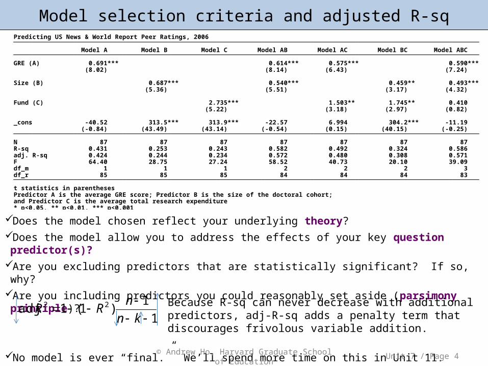
Model selection criteria and adjusted R-sq

* p<0.05, ** p<0.01, *** p<0.001and Predictor C is the average total research expenditurePredictor A is the average GRE score; Predictor B is the size of the doctoral cohort;t statistics in parentheses df_r 85 85 85 84 84 84 83 df_m 1 1 1 2 2 2 3 F 64.40 28.75 27.24 58.52 40.73 20.10 39.09 adj. R-sq 0.424 0.244 0.234 0.572 0.480 0.308 0.571 R-sq 0.431 0.253 0.243 0.582 0.492 0.324 0.586 N 87 87 87 87 87 87 87 (-0.84) (43.49) (43.14) (-0.54) (0.15) (40.15) (-0.25) _cons -40.52 313.5*** 313.9*** -22.57 6.994 304.2*** -11.19

(5.22) (3.18) (2.97) (0.82) Fund (C) 2.735*** 1.503** 1.745** 0.410

(5.36) (5.51) (3.17) (4.32) Size (B) 0.687*** 0.540*** 0.459** 0.493***

(8.02) (8.14) (6.43) (7.24) GRE (A) 0.691*** 0.614*** 0.575*** 0.590*** Model A Model B Model C Model AB Model AC Model BC Model ABC Predicting US News & World Report Peer Ratings, 2006

Does the model chosen reflect your underlying theory? Does the model allow you to address the effects of your key question predictor(s)?Are you excluding predictors that are statistically significant? If so, why?Are you including predictors you could reasonably set aside (parsimony principle)?

No model is ever “final.” We’ll spend more time on this in Unit 11.1

1)1(1adj 22

kn

nRR Because R-sq can never decrease with additional predictors, adj-R-sq

adds a penalty term that discourages frivolous variable addition.

Unit 7 / Page 4© Andrew Ho, Harvard Graduate School of Education

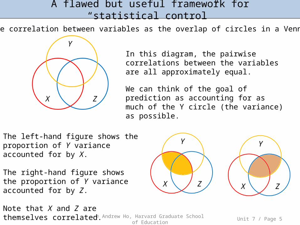
A flawed but useful framework for “statistical control”

Y

X Z

Unit 7 / Page 5© Andrew Ho, Harvard Graduate School of Education

Think of the correlation between variables as the overlap of circles in a Venn diagram:

Y

X Z

In this diagram, the pairwise correlations between the variables are all approximately equal.

We can think of the goal of prediction as accounting for as much of the Y circle (the variance) as possible.

Y

X Z

The left-hand figure shows the proportion of Y variance accounted for by X.

The right-hand figure shows the proportion of Y variance accounted for by Z.

Note that X and Z are themselves correlated.

© Andrew Ho, Harvard Graduate School of Education

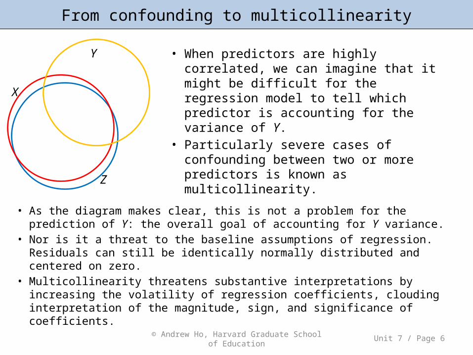
From confounding to multicollinearity

• When predictors are highly correlated, we can imagine that it might be difficult for the regression model to tell which predictor is accounting for the variance of Y.

• Particularly severe cases of confounding between two or more predictors is known as multicollinearity.

Unit 7 / Page 6

Y

X

Z

• As the diagram makes clear, this is not a problem for the prediction of Y: the overall goal of accounting for Y variance.

• Nor is it a threat to the baseline assumptions of regression. Residuals can still be identically normally distributed and centered on zero.

• Multicollinearity threatens substantive interpretations by increasing the volatility of regression coefficients, clouding interpretation of the magnitude, sign, and significance of coefficients.

The body fat example

• Predicting the percentage of body fat in 20 healthy females 25-34 years old.

• Can we predict the percentage of body fat using a much less expensive and time-consuming procedure: measuring triceps skinfold thickness (mm), thigh circumference (cm), and midarm circumference (cm)?

© Andrew Ho, Harvard Graduate School of Education Unit 7 / Page 7

20. 21.1 25.2 51 27.5 19. 14.8 22.7 48.2 27.1 18. 25.4 30.2 58.6 24.6 17. 22.6 27.7 55.3 25.7 16. 23.9 29.5 54.4 30.1 15. 12.8 14.6 42.7 21.3 14. 17.8 19.7 44.2 28.6 13. 11.7 18.7 46.5 23 12. 27.2 30.4 56.7 28.3 11. 25.4 31.1 56.6 30 10. 19.3 25.5 53.5 24.8 9. 21.3 22.1 49.9 23.2 8. 25.4 27.9 52.1 30.6 7. 27.1 31.4 58.5 27.6 6. 21.7 25.6 53.9 23.7 5. 12.9 19.1 42.2 30.9 4. 20.1 29.8 54.3 31.1 3. 18.7 30.7 51.9 37 2. 22.8 24.7 49.8 28.2 1. 11.9 19.5 43.1 29.1 bodyfat triceps thigh midarm

. list, clean

midarm 20 27.62 3.647147 21.3 37 thigh 20 51.17 5.234611 42.2 58.6 triceps 20 25.305 5.023259 14.6 31.4 bodyfat 20 20.195 5.106186 11.7 27.2 Variable Obs Mean Std. Dev. Min Max

. su

* p<0.05, ** p<0.01, *** p<0.001p-values in parentheses N 20 (0.549) (0.042) (0.723) midarm 0.142 0.458* 0.0847 1

(0.000) (0.000) thigh 0.878*** 0.924*** 1

(0.000) triceps 0.843*** 1

bodyfat 1 bodyfat triceps thigh midarm

Percentbodyfat

Tricepsskinfold

thickness(mm)

Thighcircumference

(cm)

Midarmcircumference

(cm)

10

20

30

10 20 30

15

20

25

30

15 20 25 30

40

50

60

40 50 60

20

30

40

20 30 40

Comparing regression coefficients across models

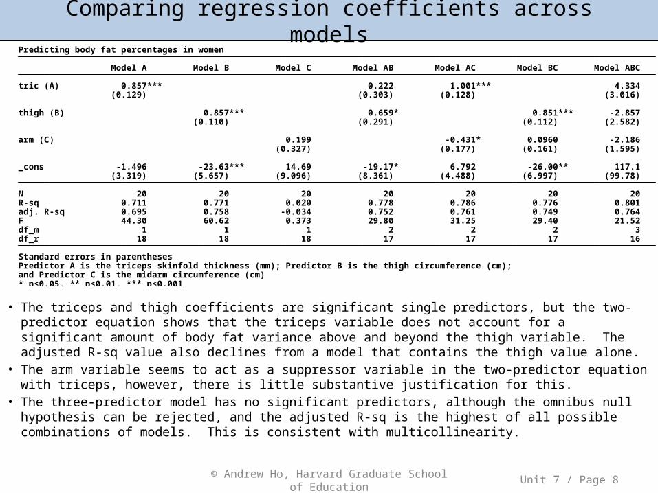
• The triceps and thigh coefficients are significant single predictors, but the two-predictor equation shows that the triceps variable does not account for a significant amount of body fat variance above and beyond the thigh variable. The adjusted R-sq value also declines from a model that contains the thigh value alone.

• The arm variable seems to act as a suppressor variable in the two-predictor equation with triceps, however, there is little substantive justification for this.

• The three-predictor model has no significant predictors, although the omnibus null hypothesis can be rejected, and the adjusted R-sq is the highest of all possible combinations of models. This is consistent with multicollinearity.

© Andrew Ho, Harvard Graduate School of Education Unit 7 / Page 8

* p<0.05, ** p<0.01, *** p<0.001and Predictor C is the midarm circumference (cm)Predictor A is the triceps skinfold thickness (mm); Predictor B is the thigh circumference (cm);Standard errors in parentheses df_r 18 18 18 17 17 17 16 df_m 1 1 1 2 2 2 3 F 44.30 60.62 0.373 29.80 31.25 29.40 21.52 adj. R-sq 0.695 0.758 -0.034 0.752 0.761 0.749 0.764 R-sq 0.711 0.771 0.020 0.778 0.786 0.776 0.801 N 20 20 20 20 20 20 20 (3.319) (5.657) (9.096) (8.361) (4.488) (6.997) (99.78) _cons -1.496 -23.63*** 14.69 -19.17* 6.792 -26.00** 117.1

(0.327) (0.177) (0.161) (1.595) arm (C) 0.199 -0.431* 0.0960 -2.186

(0.110) (0.291) (0.112) (2.582) thigh (B) 0.857*** 0.659* 0.851*** -2.857

(0.129) (0.303) (0.128) (3.016) tric (A) 0.857*** 0.222 1.001*** 4.334 Model A Model B Model C Model AB Model AC Model BC Model ABC Predicting body fat percentages in women

© Andrew Ho, Harvard Graduate School of Education

• When any two predictors are perfectly correlated, the regression procedure crashes. There are an infinite number of equations for the best-fit plane, each with different regression coefficients for and . Algebraically, if , then:

Visualizing multicollinearity

• Multicollinearity arises from an inability of the estimation procedure to decide from among a number of feasible equations for the best-fit plane.

Unit 7 / Page 9

𝑌

𝑋 1𝑋 2

• These problems occur more often than one might expect.• One might accidentally include two predictors that

are on different but linearly related scales, (meters and feet, scale scores and z-scores, frequencies and percentages).

• One might include variables that are linear combinations of other variables (try predicting a future score with a Time 1 score, a Time 2 score, and growth defined as Time 2 – Time 1).

• In perfect collinearity, Stata will spit out one of your variables in protest, “note: growth omitted due to collinearity.”

2321310

12322110

XX

XXXXY

XXXY 21022110

© Andrew Ho, Harvard Graduate School of Education

The Variance Inflation Factor (VIF)

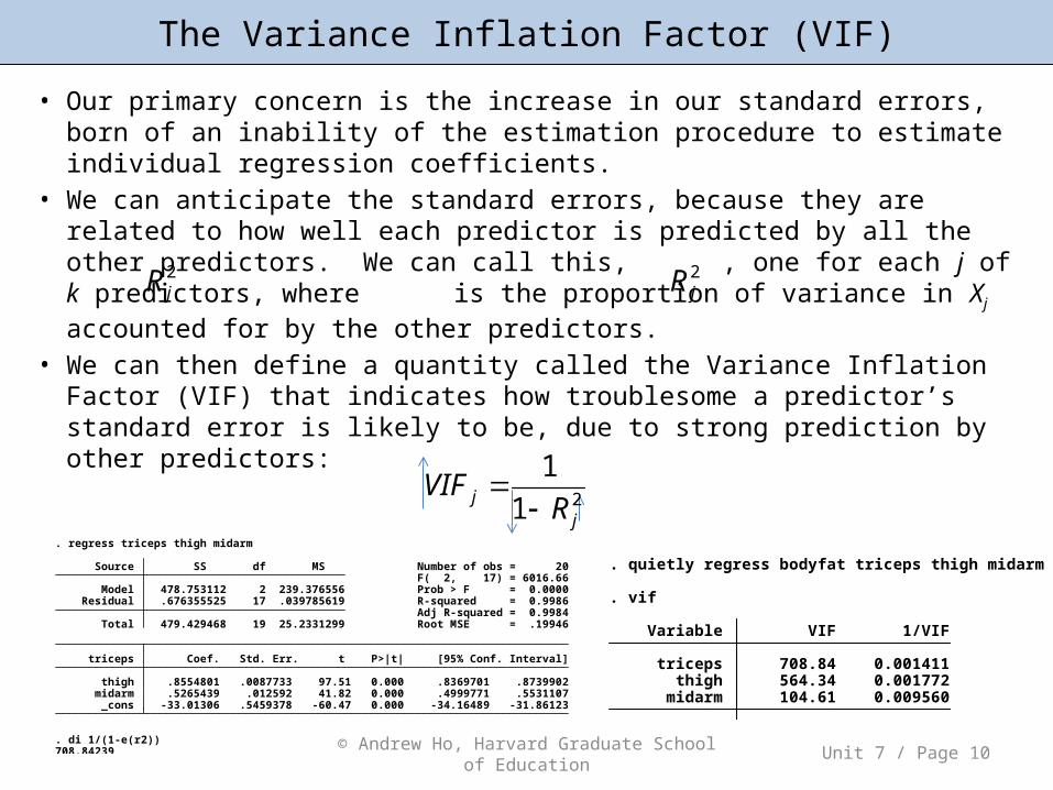
• Our primary concern is the increase in our standard errors, born of an inability of the estimation procedure to estimate individual regression coefficients.

• We can anticipate the standard errors, because they are related to how well each predictor is predicted by all the other predictors. We can call this, , one for each j of k predictors, where is the proportion of variance in Xj accounted for by the other predictors.

• We can then define a quantity called the Variance Inflation Factor (VIF) that indicates how troublesome a predictor’s standard error is likely to be, due to strong prediction by other predictors:

Unit 7 / Page 10

2jR

21

1

jj R

VIF

2jR

708.84239. di 1/(1-e(r2))

_cons -33.01306 .5459378 -60.47 0.000 -34.16489 -31.86123 midarm .5265439 .012592 41.82 0.000 .4999771 .5531107 thigh .8554801 .0087733 97.51 0.000 .8369701 .8739902 triceps Coef. Std. Err. t P>|t| [95% Conf. Interval]

Total 479.429468 19 25.2331299 Root MSE = .19946 Adj R-squared = 0.9984 Residual .676355525 17 .039785619 R-squared = 0.9986 Model 478.753112 2 239.376556 Prob > F = 0.0000 F( 2, 17) = 6016.66 Source SS df MS Number of obs = 20

. regress triceps thigh midarm

Mean VIF 459.26 midarm 104.61 0.009560 thigh 564.34 0.001772 triceps 708.84 0.001411 Variable VIF 1/VIF

. vif

. quietly regress bodyfat triceps thigh midarm

Addressing multicollinearity

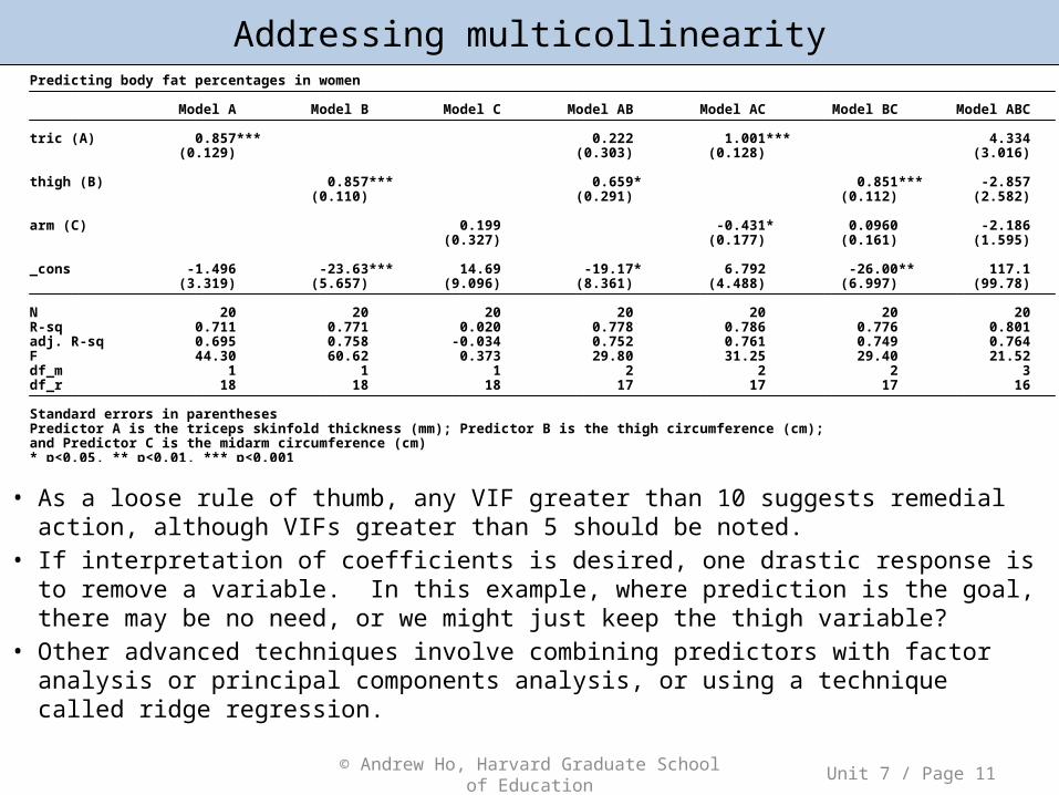
• As a loose rule of thumb, any VIF greater than 10 suggests remedial action, although VIFs greater than 5 should be noted.

• If interpretation of coefficients is desired, one drastic response is to remove a variable. In this example, where prediction is the goal, there may be no need, or we might just keep the thigh variable?

• Other advanced techniques involve combining predictors with factor analysis or principal components analysis, or using a technique called ridge regression.

© Andrew Ho, Harvard Graduate School of Education Unit 7 / Page 11

* p<0.05, ** p<0.01, *** p<0.001and Predictor C is the midarm circumference (cm)Predictor A is the triceps skinfold thickness (mm); Predictor B is the thigh circumference (cm);Standard errors in parentheses df_r 18 18 18 17 17 17 16 df_m 1 1 1 2 2 2 3 F 44.30 60.62 0.373 29.80 31.25 29.40 21.52 adj. R-sq 0.695 0.758 -0.034 0.752 0.761 0.749 0.764 R-sq 0.711 0.771 0.020 0.778 0.786 0.776 0.801 N 20 20 20 20 20 20 20 (3.319) (5.657) (9.096) (8.361) (4.488) (6.997) (99.78) _cons -1.496 -23.63*** 14.69 -19.17* 6.792 -26.00** 117.1

(0.327) (0.177) (0.161) (1.595) arm (C) 0.199 -0.431* 0.0960 -2.186

(0.110) (0.291) (0.112) (2.582) thigh (B) 0.857*** 0.659* 0.851*** -2.857

(0.129) (0.303) (0.128) (3.016) tric (A) 0.857*** 0.222 1.001*** 4.334 Model A Model B Model C Model AB Model AC Model BC Model ABC Predicting body fat percentages in women

© Andrew Ho, Harvard Graduate School of Education

Model selection philosophies (more in Unit 11)

• Different disciplines and subdisciplines have different norms driving variable and model selection.

• More substantively driven fields that typically deal with lower sample sizes tend to include predictors on theoretical grounds.– Remember that including a nonsignificant predictor can still reduce bias in

other predictors, if it really functions as a covariate in the population.• More statistically driven fields that typically deal with larger sample sizes tend to

prune predictors for parsimony and because there is limited evidence supporting the inclusion of nonsignificant variables in the absence of strong theory.

• We want you to appreciate this continuum while also emphasizing the value of sensitivity studies: coefficient comparisons across models. Regardless of your philosophy, robust interpretations of coefficients across plausible models should be reassuring, and volatility should be reported and explained substantively to the extent possible.

• Even if prediction alone is the goal, beware of chasing R-sq or even adj-R-sq blindly. This can lead to overfitting: models that fit the sample data well but do so by chasing random noise. A more parsimonious model will fit the next sample from the population better in these cases.

Unit 7 / Page 12

© Andrew Ho, Harvard Graduate School of Education

Start looking at the results sections of papers in your field

Unit 7 / Page 13

Michal Kurlaender & John Yun (2007) Measuring school racial composition and student outcomes in a multiracial society, American Journal of Education, 113, 213-242

© Andrew Ho, Harvard Graduate School of Education

Get to know the norms in your discipline

Unit 7 / Page 14

Barbara Pan, Meredith Rowe, Judith Singer and Catherine Snow (2005) Maternal correlates of growth in toddler vocabulary production in low-income families, Child Development, 76(4) 763-782

© Andrew Ho, Harvard Graduate School of Education

What are the takeaways from this unit?

Unit 7 / Page 15

• Multiple regression is a very powerful tool– The ability to estimate certain associations while accounting for others greatly expands the

utility of statistical models– It can support inferences about the effects of some predictors while holding other predictors

constant• But with great power comes great responsibility

– Coefficients and their interpretations are conditional on all the variables in a model. Inclusion or exclusion of variables can change interpretations dramatically.

– It is our responsibility to explore plausible rival models and anticipate the effects of including variables beyond the scope of our dataset.

• The pattern of correlations can help presage multiple regression results– Learn how to examine a correlation matrix and foreshadow how the predictors will behave in a

multiple regression model– If you have one (or more) control predictors, consider examining a partial correlation matrix

that removes that effect• Multicollinearity is an extreme example of confounding

– We can anticipate it with correlations but metrics like VIF are better at flagging problems.– Collinearity can be addressed by variable exclusion, variable combination, or more advanced

techniques.