unit 9: inferences for proportions and count...

1

12/15/2008 Unit 9 - Stat 571 - Ramón V. León 1

Unit 9: Inferences for Proportions and Count Data

Statistics 571: Statistical MethodsRamón V. León


Large Sample Confidence Interval for Proportion

( ) ( )ˆ ˆNote that (0,1) and (0,1) if is large

ˆ ˆ/ /ˆ ˆ ( 1- , 10 and 10)

p p p pN N n

pq n pq nq p np nq

− −≈ ≈

= ≥ ≥

Confidence interval for p:

2 2ˆ ˆ ˆ ˆˆ ˆpq pqp z p p zn nα α− ≤ ≤ +

( )2 2

ˆ1

ˆ ˆp p

P z zpq nα α α

⎛ ⎞−− ≤ ≤ ≈ −⎜ ⎟⎜ ⎟⎝ ⎠

It follows that:

2


A Better Confidence Interval for Proportion

CI for p:

( )2 2

ˆ1

p pP z z

pq nα α α⎛ ⎞−− ≤ ≤ ≈ −⎜ ⎟⎜ ⎟⎝ ⎠

Use this probability statement

Solve for p using quadratic equation


3


CI for Proportion in JMP

Value column has two categories. Can you imagine a situation where one would have more categories in this column?

= 0.45 x 800= 0.55 x 800

Arbitrary choice of names


CI for Proportion in JMP

4


Sample Size Determination for a Confidence Interval for Proportion

Want (1-α)-level two-sided CI:

2

22

ˆ ˆˆ where E is the margin of error. Then .

ˆ ˆSolving for gives (Formula 9.4)

pqp E E zn

zn n pq

E

α

α

± =

⎛ ⎞= ⎜ ⎟⎝ ⎠

22

1 1 1Largest value of so conservative sample size is:2 2 4

1 (Formula 9.5)4

pq

zn

Eα

⎛ ⎞⎛ ⎞= =⎜ ⎟⎜ ⎟⎝ ⎠⎝ ⎠

⎛ ⎞= ⎜ ⎟⎝ ⎠


Example 9.2: Presidential Poll

Threefold increase in precision requires ninefold increase in sample size

21.96 1 96040.01 4

n ⎛ ⎞= =⎜ ⎟⎝ ⎠

1067.11 9 9604× =

5


Largest Sample Hypothesis Test on Proportion

0 0 1 0: vs. : H p p H p p= ≠

Best test statistics: 0

0 0

p̂ pzp q n−

=

•Dual relationship between CI and test of hypothesis holds if thebetter confidence interval is used.

•There is an exact test that can be used when the sample size is small (given in Section 9.1.3). We do not cover it.


Basketball Problem: z-test

2.182

6


Test for Proportion in JMP: Baseball Problem

“Value” has two categories.


Test for Proportion in JMP: Basketball Problem

7


Sample Size for Z-Test of Proportion0 1 0: vs. :oH p p H p p≤ >

0

1 0

1 02

0 0 1 1

2

Suppose that the power for rejecting must be atleast 1- when the true proportion is .Let . Then

Replace by for two-sided test sample size.

Hp p p

p p

z p q z p qn

z z

α β

α α

βδ

δ

= >= −

⎡ ⎤+= ⎢ ⎥⎢ ⎥⎣ ⎦

0

0 0

Test based on:p̂ pzp q n−

=


Example 9.4: Pizza Testing

0

1

: Can't tell two pizzas Apart, : Can tell pizzas apart

HH

.10, We wants =.25 when 0.5 0.1 pα β= = ±

( )( ) ( )( )

2

2 0 0 1 1

21.645 .5 .5 0.675 .6 .4

132.98 1330.1

z p q z p qn α β

δ

⎡ ⎤+= ⎢ ⎥⎢ ⎥⎣ ⎦

⎡ ⎤+⎢ ⎥= = ≈⎢ ⎥⎣ ⎦

8


Multinomial Test of Proportions


Multinomial Test in JMP

Observed count does not exhibit significant deviation from the uniform model.

Note that one could have gotten confidence intervals

9


Comparing Two Proportion: Independent Sample Design

1 1 1 1 2 2 2 2

1 2 1 2

1 1 2 2

1 2

If , , , 10, thenˆ ˆ ( ) (0,1)

ˆ ˆ ˆ ˆ

n p n q n p n qp p p pZ N

p q p qn n

≥− − −

= ≈+

1 1 2 2 1 1 2 21 2 2 1 2 1 2 2

1 2 1 2

ˆ ˆ ˆ ˆ ˆ ˆ ˆ ˆˆ ˆ ˆ ˆp q p q p q p qp p z p p p p zn n n nα α− − + ≤ − ≤ − + +

Confidence Interval:


Test for Equality of Proportions (Large n) Independent Sample Design

0 1 2 1 1 2: vs. :H p p H p p= ≠

1 2

1 2

1 1 2 2

1 2 1 2

ˆ ˆTest statitics:

1 1ˆ ˆ

ˆ ˆˆwhere

p pz

pqn n

n p n p x ypn n n n

−=

⎛ ⎞+⎜ ⎟

⎝ ⎠+ +

= =+ +

•There is small sample test called Fisher’s exact test. See JMP output latter.•See Example 9.5 for application to the Salk Polio Vaccine Trial•There a test for Matched Pair Design in Section 9.2.2. Please read Example 9.9 to see its application for testing the effectiveness of presidential debates. Do voters change their minds about candidates because of debates?

10


Example 9.6 –Comparing Two Leukemia Therapies


Test for Equality of

Proportions in JMP:

Example 9.6

11


Example 9.6 JMP Output

Res

ult

0.00

0.25

0.50

0.75

1.00

Prednisone Prednisone + VCR

Drug Group

Failure

Success


Test for Equality of Proportions

in JMP

ModelErrorC. TotalN

Source 1 61 62 63

DF 2.600496 26.575470 29.175966

-LogLike0.0891

RSquare (U)

Likelihood RatioPearson

Test 5.201 5.507

ChiSquare 0.0226 0.0189

Prob>ChiSq

LeftRight2-Tail

Fisher's Exact Test 0.9958 0.0254 0.0323

Prob

Tests

Recall that the P-value of the two-sided z-test was calculated to be 0.019

z2 = (-2.347)2

Less significantresult

12


Inferences for Two-Way Count Data

Sampling Model 1: Multinomial Model (Total Sample Size Fixed)Sample of 901 from a single population that is then cross-classified

The null hypothesis is that X and Y are independent:

0 . .: ( , ) ( ) ( ) for all i, jij i jH p P X i Y j P X i P Y j p p= = = = = = =


Sampling Model 1 (Total Sample Size Fixed)

1 1

62 206 62 206Estimated Expected Frequency = 901 14.18901 901 901

np p• •

×⎛ ⎞⎛ ⎞ = =⎜ ⎟⎜ ⎟⎝ ⎠⎝ ⎠

=(Cell 1,1)

13


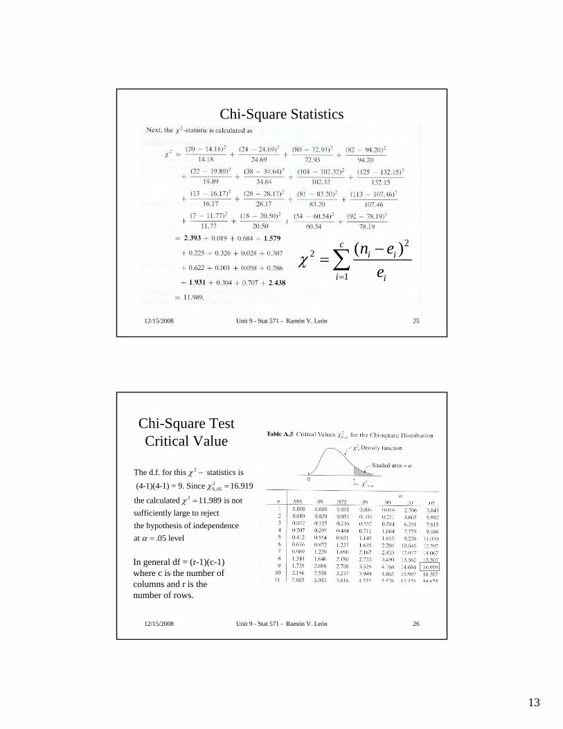
Chi-Square Statistics

22

1

( )ci i

i i

n ee

χ=

−=∑


Chi-Square Test Critical Value

2

29,.05

2

The d.f. for this statistics is (4-1)(4-1) = 9. Since 16.919

the calculated 11.989 is not sufficiently large to reject the hypothesis of independenceat .05 level

χχ

χ

α

−

=

=

=

In general df = (r-1)(c-1) where c is the number of columns and r is the number of rows.

14


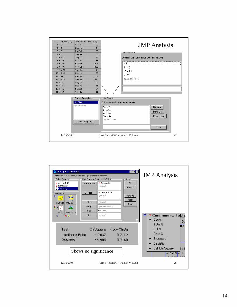
JMP Analysis


JMP Analysis

Shows no significance

15


JMP Analysis

Note that most of the contribution to the chi-square statistics comes from the cornercells. Lack of significancein the chi-square statisticsis the result of the lowcontribution to the chi-square statistic comingfrom the center cells.


JMP Analysis

Restricting our chi-square analysis to the corner cellsshows a strong relationshipbetween income and levelof satisfaction.

16


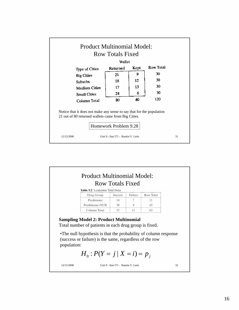
Product Multinomial Model:Row Totals Fixed

Homework Problem 9.28

Notice that it does not make any sense to say that for the population 21 out of 80 returned wallets came from Big Cities.


Product Multinomial Model:Row Totals Fixed

Sampling Model 2: Product MultinomialTotal number of patients in each drug group is fixed.

•The null hypothesis is that the probability of column response (success or failure) is the same, regardless of the row population:

0 : ( | ) jH P Y j X i p= = =

17


Chi-Square Statistics

22

1

( )ci i

i i

n ee

χ=

−=∑


JMP Analysis

18


JMP Analysis

( )22

Recall Slide 19:

2.347 5.5084z = − =


Remarks About Chi-Square Test

• The distribution of the chi-square statistics under the null hypothesis is approximately chi-square only when the sample sizes are large– The rule of thumb is that all expected cell counts should be greater

than 1 and – No more than 1/5th of the expected cell counts should be less than

5.

• Combine sparse cell (having small expected cell counts) with adjacent cells. Unfortunately, this has the drawback of losing some information.

19


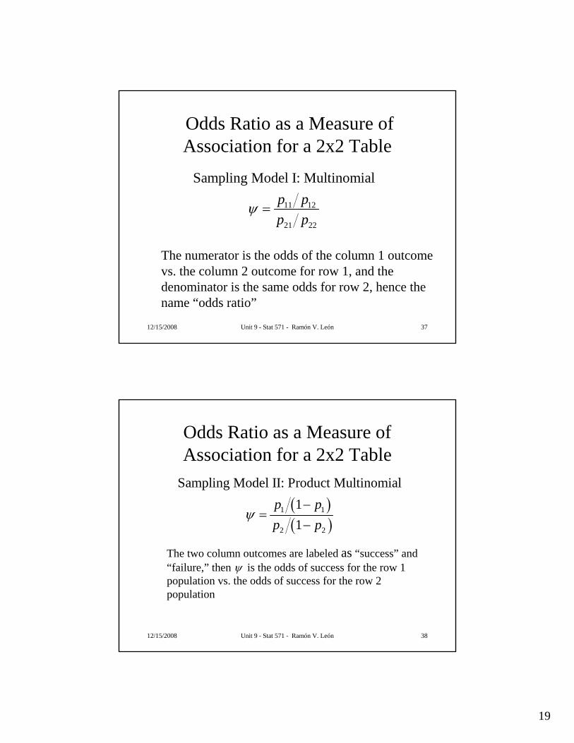
Odds Ratio as a Measure of Association for a 2x2 Table

11 12

21 22

Sampling Model I: Multinomialp pp p

ψ =

The numerator is the odds of the column 1 outcome vs. the column 2 outcome for row 1, and the denominator is the same odds for row 2, hence the name “odds ratio”


Odds Ratio as a Measure of Association for a 2x2 Table

( )( )

1 1

2 2

Sampling Model II: Product Multinomial11

p pp p

ψ−

=−

The two column outcomes are labeled as “success” and “failure,” then ψ is the odds of success for the row 1 population vs. the odds of success for the row 2 population

20


Odds Ratio as a Measure of Association

for a 2x2 Table

11 21

11 12 21 22

12 22

11 12 21 22

11 12 11 22

21 22

14 3814 3821 42ˆ

7 4 7 421 42

ˆ

n nn n n n

n nn n n n

n n n nn n n

ψ

ψ

⎛ ⎞ ⎛ ⎞⎛ ⎞ ⎛ ⎞ ⎛ ⎞ ⎛ ⎞⎛ ⎞ ⎛ ⎞⎜ ⎟ ⎜ ⎟⎜ ⎟ ⎜ ⎟ ⎜ ⎟ ⎜ ⎟⎜ ⎟ ⎜ ⎟+ + ⎛ ⎞ ⎛ ⎞⎝ ⎠ ⎝ ⎠ ⎝ ⎠ ⎝ ⎠⎜ ⎟ ⎜ ⎟ ⎜ ⎟ ⎜ ⎟= = = ⎜ ⎟ ⎜ ⎟⎜ ⎟ ⎜ ⎟⎛ ⎞ ⎛ ⎞ ⎛ ⎞ ⎛ ⎞ ⎝ ⎠ ⎝ ⎠⎜ ⎟ ⎜ ⎟⎜ ⎟ ⎜ ⎟⎜ ⎟ ⎜ ⎟ ⎜ ⎟ ⎜ ⎟⎜ ⎟ ⎜ ⎟⎜ ⎟ ⎜ ⎟ ⎝ ⎠ ⎝ ⎠+ + ⎝ ⎠ ⎝ ⎠⎝ ⎠ ⎝ ⎠⎝ ⎠ ⎝ ⎠

= =12 21

14 4 0.210538 7

Confidence Inteval: [0.053,0.831]n

×= =

×


Case-Control Studies: The Odds Ratio Approximates the Relative Risk if the Disease is Rare

21


JMP Output for Case-Control Study


How to Do It in JMP

22



23



Do You Need to Know More?578 Categorical Data Analysis (3) Log-linear analysis of multidimensional contingency tables. Logistic regression. Theory, applications, and use of statistical software. Prereq: 1 yr graduate-level statistics, regression analysis and analysis of variance, or consent of instructor. Sp

Reference: “An Introduction to Categorical Data Analysis”by Alan Agresti. Wiley.

unit 9: inferences for proportions and count...

Documents