UNIT I

GENERAL FOUNDATION OF MANAGERIAL ECONOMICS

Economics can be broadly divided into two categories namely, microeconomics

and macroeconomics. Macroeconomics studies the economic system in

aggregate on the other hand micro-economics studies the behavior of an

individual decision-making economic unit like a firm, a consumer, or an

individual supplier of some factor of production.

Macroeconomics relates to issues such as determination of national

income, savings, investment, employment at aggregate levels, tax collection,

government expenditure, foreign trade, money supply and price level, etc.

In simple terms, managerial economics can be taken as applied micro-

economics. It is an application of that part of micro-economics which is directly

related to decision making by a manager. Thus, managerial economics analyses

the process through which a manager uses economic theories to address the

complex problems of business world, and then take ‘rational’ decisions in such

a way that the preconceived objectives of the concerned firm may be attained

(Barla: 2000).

Like an economy, the manager of a firm also faces five basic issues:-

(1) Choice of product, i.e., the products a firm has to produce - A manager has to

allocate the available resources so as to maximize the profit of the firm.

(2) Choice of inputs – After determining the profit maximising level of output,

the manager has to identify the input-mix which would produce the profit

maximizing level of output at a minimum cost.

(3) Distribution of the firms’ revenue – The revenue received by the firm

through sales has to be distributed in a just and fair manner by the manager.

Workers, owner of factory building, bankers, and all those who have contributed

their materials and services in the process of production, storage and

transportation, have to be paid remunerations according to the terms and

conditions already agreed upon. The residual after such payments constitutes

the firm’s profit which has to be distributed among the owners of the firm after

tax payment.

(4) Rationing - This constitutes an important function of a manager. He/she

should utilize the scarce resources optimally, which involves expenditure. As

the manager has to often look after several plants simultaneously, he/she must

prioritize not only the allocation of resources but also the time.

(5) Maintenance and expansion – In addition, the manager has to plan strategies

to ensure that the level of output is maintained, the efficiency of the firm is

retained over time, and also to plan the future expansion of the firm. Expansion

of the firm involves making adequate provisions for mobilizing additional

capital from the market and/or borrowing money from banks. A dynamic

manager always aspires to expand the firm’s scale of operation so as to increase

the profits.

1.1 Circular Flow of Economic Activities

Economic analysis attempts to explain the working of economic systems.

Assume a simple economic system consisting of two sectors, whose activities

are systematically connected with one another. (there is no link between both the

sentence) The economic activities performed by economic agents are generally

classified into three inter-related activities:-

(a) Supplying factor inputs like land, labour, capital, organisation and

enterprise, which enable the agents to earn income which in turn could be used

for purchasing consumable goods;

(b) Using the factor inputs like raw materials, machines, labour, land,

etc., for producing goods to be supplied to the consumers; and

(c) Providing intangible and specialized services directly to the people

(example, lawyers, teachers, doctors, and porters) or working for the

government (example, soldiers, judges, police, etc.).

The nature and dimensions of economic activities are generally determined by

the extent of overall economic development. For instance, a developed

economic system like that of the United States or Japan, has more specialized

activities and division of labour, as compared to a traditional economic system.

In an extremely primitive economic system, the extent of interdependence

among economic agents tends to be limited, with some kind of division of

labour in them.

The extent of monetization and foreign trade also determine the nature

and scope of economic activities in a country. Foreign trade adds various

dimensions to the process of identification of economic activities. Further, the

extent of government intervention also complicates this process. Hence, to

study the flow of income among different economic agents, a simplified

economy with non-existent government economic activities and foreign trade

may be considered, wherein the inflow and outflow of income among different

economic agents are always equal.

households firms

Commodities

expenditure on commodities

factor services

money incomeDiagram – 1 Circular flows in a two-sector economy

1.2 Forms of Organisation

In modern times, organisation of business assume several forms, viz.,

sole proprietorship, individual entrepreneur or one-man business, partnership,

joint–stock companies, industrial combination, co-operative enterprises and state

enterprises.

a) Individual Entrepreneur: Under the ‘one-man’ concern, organiser invests

his/her own capital and may also borrow some. He/she rents a shop and

employs a worker, if necessary. He/she personally make purchases and attend to

the sales, and who also takes the entire risks. Thus, an entrepreneur organizes,

directs all economic activity and takes the full risks, and is the sole proprietor.

b) Partnership: In partnership firm, two, three or more people join together,

contribute capital, and share the profits and risks of losses in agreed proportions.

c) Joint-stock company: It is the most important type of business organisation

today. It overcomes the disadvantages of the partnership arising out of small

financial resources and limited business talent.

d) Co-operative enterprise: They are of two types –

1) Producer’s cooperation, and

2) Consumer’s cooperation.

1) Producers cooperation: Under it, the workers take up the entrepreneurial

work; contribute some capital and borrow the rest; elect their own foreman and

managers and employ other staff. After all expenses on rent, capital, salaries

and wages, the profits are divided by the workers. This type of co-operation is

called the productive co-operation or producer’s co-operation.

ii) Consumer’s cooperation: Under it, the consumers of a region contribute small

shares of capital and start a store. These co-operative stores buy goods from

wholesalers or, and sells them to the members at the market price. The profits

are shared by the members in proportion to their purchases or, commonly, in

proportion to their capital share. Usually, the capital share is contributed equally

and therefore profits are also equally shared by the members.

State enterprise: The organisation of state enterprise is similar to that of the

private enterprises. It consists of general manager, foremen, works manager,

accountants, treasurer, departmental heads, etc. It functions in a similar way like

a joint-stock company. But, the fundamental difference is that all its employees

are government servants with fixed tenure and pension benefits on retirement.

The capital comes from the state revenue, which are attributed by the tax-payers.

Therefore, the profit, if any, goes to the state.

Public enterprises: Public enterprises may be in the form of

i) Departments, i.e., run by a government department, e.g., railways and postal

and telegraph in India,

ii) Corporation, e.g., Life Insurance Corporation of India which is established by

a special Act of Parliament, and

iii) Limited Liability Company registered under the Companies Act.

1.2 Objectives of the Firm

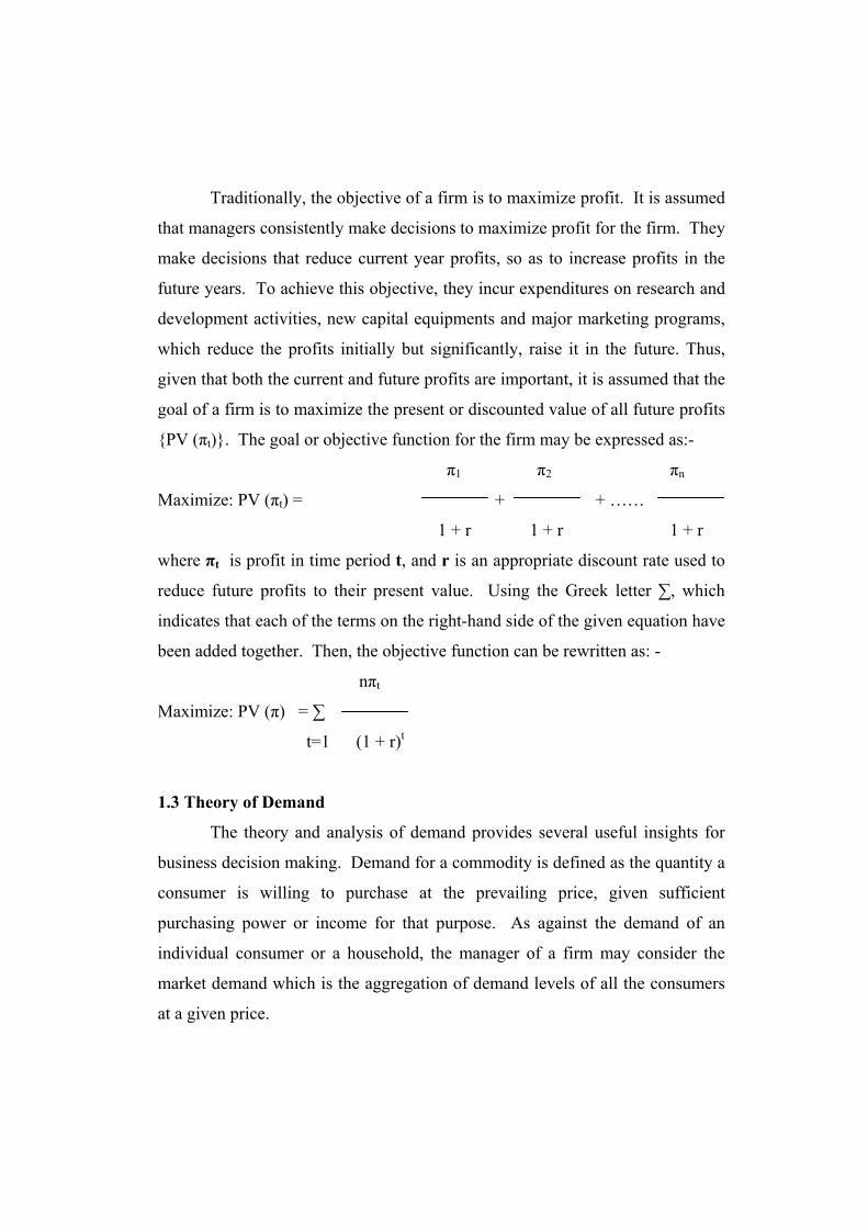
Traditionally, the objective of a firm is to maximize profit. It is assumed

that managers consistently make decisions to maximize profit for the firm. They

make decisions that reduce current year profits, so as to increase profits in the

future years. To achieve this objective, they incur expenditures on research and

development activities, new capital equipments and major marketing programs,

which reduce the profits initially but significantly, raise it in the future. Thus,

given that both the current and future profits are important, it is assumed that the

goal of a firm is to maximize the present or discounted value of all future profits

PV (πt). The goal or objective function for the firm may be expressed as:-

π1 π2 πn

Maximize: PV (πt) = + + ……

1 + r 1 + r 1 + r

where πt is profit in time period t, and r is an appropriate discount rate used to

reduce future profits to their present value. Using the Greek letter ∑, which

indicates that each of the terms on the right-hand side of the given equation have

been added together. Then, the objective function can be rewritten as: -

nπt

Maximize: PV (π) = ∑

t=1 (1 + r)t

1.3 Theory of Demand

The theory and analysis of demand provides several useful insights for

business decision making. Demand for a commodity is defined as the quantity a

consumer is willing to purchase at the prevailing price, given sufficient

purchasing power or income for that purpose. As against the demand of an

individual consumer or a household, the manager of a firm may consider the

market demand which is the aggregation of demand levels of all the consumers

at a given price.

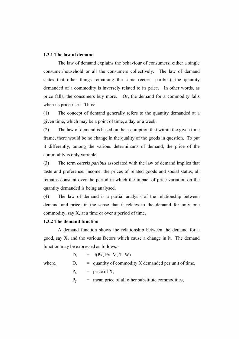
1.3.1 The law of demand

The law of demand explains the behaviour of consumers; either a single

consumer/household or all the consumers collectively. The law of demand

states that other things remaining the same (ceteris paribus), the quantity

demanded of a commodity is inversely related to its price. In other words, as

price falls, the consumers buy more. Or, the demand for a commodity falls

when its price rises. Thus:

(1) The concept of demand generally refers to the quantity demanded at a

given time, which may be a point of time, a day or a week.

(2) The law of demand is based on the assumption that within the given time

frame, there would be no change in the quality of the goods in question. To put

it differently, among the various determinants of demand, the price of the

commodity is only variable.

(3) The term ceteris paribus associated with the law of demand implies that

taste and preference, income, the prices of related goods and social status, all

remains constant over the period in which the impact of price variation on the

quantity demanded is being analysed.

(4) The law of demand is a partial analysis of the relationship between

demand and price, in the sense that it relates to the demand for only one

commodity, say X, at a time or over a period of time.

1.3.2 The demand function

A demand function shows the relationship between the demand for a

good, say X, and the various factors which cause a change in it. The demand

function may be expressed as follows:-

Dx = f(Px, Py, M, T, W)

where, Dx = quantity of commodity X demanded per unit of time,

Px = price of X,

Py = mean price of all other substitute commodities,

M = consumer’s income,

T = taste, and

W = wealth of the consumer

Of the variables mentioned, tastes are difficult to quantify, whereas wealth does

not have a direct influence on the demand Dx. Hence, T and W are held

constant, and Dx is assumed to be a function of Px, Py and M only.

Demand functions are generally homogenous of degree zero. Homogeneity

means that changes in all the independent variables, namely, Px, Py and M are

uniform. If the degree of a homogenous function is zero, then it would imply

that when all prices and income change in the same proportion, Dx would

remain unchanged (Barla: 2000).

Py and M are generally assumed to be the parameters. For simplicity, the

demand for X is assumed to be a function of only Px. The quantity demanded

and price has an inverse relationship, except in the case of a Giffen good. The

demand curve for a Giffen good is upward sloping, indicating that the price and

quantity demanded move in the same direction. Meanwhile, the demand curve

for a normal commodity is negatively sloped. The slope of the curve, however,

depends upon the price elasticity of demand for the commodity.

The demand for a commodity X, depends on its own price Px, the price

of other substitute good (Py), consumer’s income, tastes and preference, etc. In

reality however, demand depends upon numerous factors. The main

determinants of demand are as follows:-

a. Price (Px) - As already discussed, the price of a commodity and its demand

are inversely related. Hence the negative (inverse) slope of the demand curves.

b. Price of other associated good (Py): A change in Py also influences the

change in Dx. However, the direction of such change depends upon the nature

of relationship between the two goods, namely X and Y:

i) X and Y are complementary goods, when both goods satisfy a single want.

Eg. ink and pen, milk and sugar, car and petrol, etc. When price of Y rises, the

consumer will buy less of Y and also less of X, although the price of X remains

unchanged. Thus, Dx and Py , are negatively related.

ii) X and Y are substitutes, if the consumer can use more of X at the cost of Y,

or vice versa. That is, with a fall in Py, the consumer would buy more of Y

because it has become cheaper compared to X. Therefore, the demand for X

will fall and that of Y will increase. For e.g., if the price of apple falls then it

would induce the buyers to buy more. Besides, many buyers of orange may also

switch over to apple, even though the price of orange has not changed.

iii) When X and Y have no relationship, the two commodities are said to be

independent. For example, the demand for wheat and milk has no relationship.

Under such a situation, even if the price of X ( Px) falls significantly, demand for

Y (Dy) remains unchanged.

c. Income of the consumer (M) - With an increase in the income, of a consumer,

the demand also increases. Hence, the demand curve for X will have a positive

slope in relation to income. However, for an inferior good, an increase in

income would result in buying smaller quantities of it. Therefore, the demand

curve for an inferior good is negatively sloped in relation to income. For eg.,

ragi is inferior to rice or wheat for consumption.

d. Status of the consumer – Often, even when Px, Py and M are constant, the

consumer’s status in the society induces him/her to buy less or more of a good.

They have to maintain certain level of living standards, regardless of the

problems like that of incidence of loans taken, etc.

e. Demonstration effect – Sometimes, a consumer is motivated to buy some

commodity not because it has become cheaper or the income has increased, but

because the neighbours have purchased it. This is also called as the

“Bandwagon effect”. According to it, demand for X is determined not by its

utility, price or income, but by what other consumers in the society are doing.

On the other hand, there are also consumers who like to behave differently from

the others. For instance, when all other consumers buy more units of X when Px

falls, such consumers prefer to buy less of X. This is known as the “Snob

effect”.

f. Seasonal variations in demand – The demand for a good also rise or falls

according to the variations in temperature or climate conditions. Demand for air

conditioners, ice cream, cool drinks, etc, are extremely high in summers,

whereas demand for blankets and woolens are low.

g. Spatial variations in demand – Demand for a good also varies according to the

place or profession in which a consumer is engaged.

h. Taste of the consumer – The demand for a good is also determined by the

taste and preference of a consumer. Other things remaining constant, a

consumer would buy more or less of a good depending upon his/her choice or

preference function. A consumer may like coffee over tea, while another may

prefer tea over coffee. Thus, a consumer’s taste is also an important determinant

of demand for a commodity.

1.3.3 Derivation of demand curves

Other things remaining the same, a demand curve is negatively sloped due to the

law of diminishing marginal utility. This law of diminishing marginal utility

states that as more and more units of the same commodity initially are consumed

without any time gap, then the total utility (TU) derived increases at an

increasing rate, then starts increasing at a decreasing rate from the point of

inflection, becomes maximum and then starts declining. A consumer gets

maximum utility from the consumption of a commodity X, when its marginal

utility (MUx) is equal to Px, i.e., MUx = Px.

Marginal utility (MU) refers to the additional utility derived by the consumer

from the consumption of an additional unit of commodity to the total units

consumed. It starts from the origin and becomes maximum at the point of

inflection, after which, it starts declining and becomes zero when total utility is

maximum. This is shown by diagram 2.

Quantity

MUx = 0

MUx > 0Inflection

MUx < 0

TUX

0

Diagram-2: Law of Diminishing Marginal Utility

TUx/ M

Ux

MUX

Only the positive slope of the MUX curve is considered for the derivation of the

demand curve DX, as there can be no negative demand. A demand curve may be

derived from the negative slope of the MUX curve, and the consumer

equilibrium condition MUx=Px. By this logic, the Y axis represents Px, which is

represented MUx in diagram -2. This is shown in the following diagram.

D

D

Y

X2X1

Px2

Px1

0

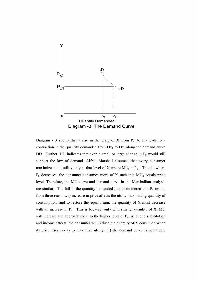
Quantity DemandedDiagram -3: The Demand Curve

Diagram - 3 shows that a rise in the price of X from Px1 to Px2 leads to a

contraction in the quantity demanded from Ox1 to Ox2 along the demand curve

DD. Further, DD indicates that even a small or large change in Px would still

support the law of demand. Alfred Marshall assumed that every consumer

maximizes total utility only at that level of X where MUx = Px . That is, where

Px decreases, the consumer consumes more of X such that MUx equals price

level. Therefore, the MU curve and demand curve in the Marshallian analysis

are similar. The fall in the quantity demanded due to an increase in Px results

from three reasons: i) increase in price affects the utility maximizing quantity of

consumption, and to restore the equilibrium, the quantity of X must decrease

with an increase in Px. This is because, only with smaller quantity of X, MU

will increase and approach close to the higher level of Px; ii) due to substitution

and income effects, the consumer will reduce the quantity of X consumed when

its price rises, so as to maximize utility; iii) the demand curve is negatively

sloping demand due to the rise in consumption as a result of a fall in price, or

conversely, due to fall in consumption when price increases.

When there are two goods namely X and Y, then the ratio of their marginal

utilities must be equal to the ratio of their respective prices. This is known as

the law of equi-marginal utility maximization. The consumer is in equilibrium

when the ratio of marginal utility and prices for all the goods is equal, i.e.,

MUx MUy MUx Px

= or =

Px Py MUy Py

The consumer maximizes utility by buying certain combination of X and Y. If

Px increases and the consumer consumes the same quantity of X, thus holding

the level of marginal utility of X at the original level, then equilibrium will be

disturbed, i.e.

MUx MUy

<

Px Py

Thus, if in spite of a rise in the price of X, the quantity demanded is held

constant, the marginal utility of Y will change due to a decrease in its quantity

because the consumer now spends more on X. Then, the consumer no longer

maximizes utility. For maximization of utility, the consumer has to reduce the

quantity of X in response to the increase in Px. Thus, when price increases, a

consumer can maximize utility only by reducing the quantity demanded.

Conversely, the quantity demanded has to increase when the price of X falls. In

the process, the equilibrium is restored at a new equilibrium at a new

combination of X and Y.

1.3.4 Demand schedule

A demand schedule shows the list of prices and the corresponding quantities of a

commodity. While preparing the demand schedule, it is assumed that the

marginal utility of money is constant and that the quantity demanded depends

only on price.

1.3.5 Elasticity of demand

In economics, the term elasticity measures a proportionate (percentage) change

in one variable to a proportionate (percentage) change in another variable. In

other words, it measures the responsiveness of the dependent variable to a given

change in one of the independent variables, other variables remaining constant.

Elasticity of demand is the responsiveness of the quantity demanded to a given

change in the price of a commodity, the prices of other commodities and

consumer’s income remaining the same. The elasticity (e) of X with respect to Y

may be written as: -

percentage change in X

Exy =

percentage change in Y

∆X/X

or, Exy =

∆Y/Y

Given the demand function: -

Dx = f (Px, Py, M)

Where, Dx = quantity of X demanded by a consumer; Px = price of X; Py = the

(weighted) price of all other commodities; and M = consumer’s income.

Demand (Dx) responds to a given change in each of these independent

variables, when the other two variables are held constant. For the concept of

elasticity of demand to be meaningful, a direct reference has to be made to the

nature of change in the independent variable (Px, Py, or M) although their

relative significance may be different in different context.

Since demand varies with fluctuations in different variables, there are different

kinds of demand elasticities, one with respect to each of the causal variable. In

modern analysis of consumer behaviour, the important demand elasticities of

significance are:-

(a) Price elasticity of demand,

(b) Cross elasticity of demand,

(c) Income elasticity of demand, and

(d) Promotional elasticity of demand

(a) Price elasticity of demand:

Price elasticity of demand measures the responsiveness or percentage change in

demand to a given percentage change in price, holding the other determinants of

demand, namely other prices (Py) and consumer’s income (M) constant. This

elasticity is also known as ‘own elasticity’ Due to the negative relationship

between demand and price, the coefficient of price elasticity has a negative sign,

which in practice is generally ignored.

Price elasticity may be measured under two alternative conditions (i) when the

change in price is very small, and (ii) when price variation is finite.

(a) when change in price is very small or infinitesimal, point elasticity method

of measurement is used: -

dDx Px

Exx = .

DPx Dx

where Exx = the price elasticity; dDx /dPx = change in demand with respect to a

change in price; Px = original price; and Dx = original quantity of demand.

Algebraically, dDx/dPx is the first derivative of demand function with respect to

price.

(b) When change in price is finite, arc method of measurement is used. Here,

rather than taking the first derivative of demand function, an attempt is made to

measure the elasticity of demand in relation to a finite change in price using the

following formula: -

∆Dx Px1 + Px2

Exx = .

∆Px Dx1 + Dx2

where X1 and Y1 = the values of X and Y at point A; and X2 and Y2 = values at

point B.

While the first part of formula i.e. ∆Dx /∆Px , measures the change between

the new and previous levels of demand in response to a finite variation in price,

the second part represents the summation of the two prices divided by the sum

total of the two levels of demand.

Both the methods of measuring price elasticity (point and arc) are useful.

While point elasticity is used to find out a change in one variable in relation to a

small change in the other variable, arc elasticity is used to find out a change in

one variable due to a large change in the other variable. For example, to find the

effect of a price change from Rs. 5 to Rs. 4.80 per unit on demand, the point

elasticity would be more appropriate, whereas if the change is from Rs. 20 to Rs.

15 per unit on demand, then arc elasticity would be more suitable. The

significance of both point and arc elasticities methods arise from the fact that

elasticities are independent of the unit of measurement. This makes the use of

elasticities popular in demand studies, as the variables in a demand function are

measured in different units which makes the analysis of their marginal effects

difficult.

The categories of price elasticity are: -

(i) Perfectly elastic demand;

(ii) Highly elastic demand;

(iii) Unit elasticity of demand;

(iv) Inelastic demand; and

(v) Perfectly inelastic demand

All these elasticities can be computed both at different points on a demand

curve, and also at a given arc. For simplicity, the point definition formula is

used to express price elasticity of demand.

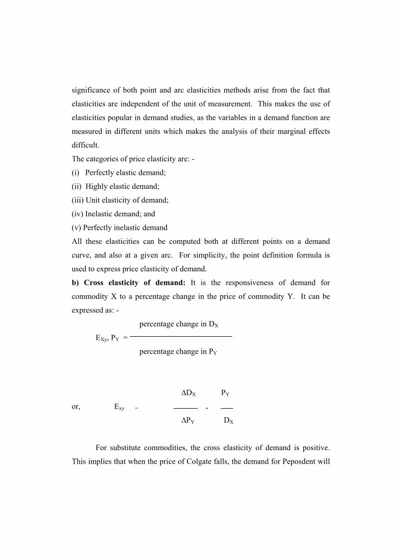
b) Cross elasticity of demand: It is the responsiveness of demand for

commodity X to a percentage change in the price of commodity Y. It can be

expressed as: -

percentage change in DX

EXy, PY =

percentage change in PY

∆DX PY

or, Exy = .

∆PY DX

For substitute commodities, the cross elasticity of demand is positive.

This implies that when the price of Colgate falls, the demand for Peposdent will

fall, as the two commodities are substitutes. When two commodities are

complements, the cross elasticity of demand will be negative. This indicates

that when the price of coffee falls, the quantity demanded of sugar will go up as

the two goods are complementary. Thus, while the signs of cross elasticity

show whether two commodities are substitutes or complements, their magnitude

indicate the degree of their relationship. The greater the cross elasticity, the

more closely related the two goods are. If the two goods have no relationship,

the cross elasticity between them will be zero. The concept of cross elasticity of

demand is useful in measuring the interdependence of demand for a commodity

and the prices of its related commodities. Its knowledge thus helps a firm to

estimate the likely effects sales of pricing decisions of its competitors on its own

sales.

c ) Income Elasticity of Demand

Income elasticity of demand (eD X, I) measures the responsiveness of

demand for a commodity, say X (DX) to a change in consumers’ income (I). It

can be computed from the following formula:

percentage change in DX

EXI =

percentage change in I

∆DX/DX

=

∆ I/I

∆DX I

or EXI = .

∆ I DX

For superior goods income elasticity is positive, whereas for inferior

good it is negative. Positive income elasticity can assume three forms: greater

than unity (one) elasticity, unity elasticity and less than unity elasticity. When a

change in income results in a direct and more than proportionate change in the

quantity demanded, the income elasticity is said to be positive and more than

unity. Luxury goods are its example. When a change in income leads to a direct

and proportionate change in the quantity demanded, then it is known as positive

and unit income elasticity. Its examples include semi-luxury and comfort goods.

When an increase in income results in a less than proportionate increase in

quantity demanded, then the elasticity is positive and less than unity. Necessary

goods fall under this category. The income elasticity is negative when an

increase in income leads to a decrease in quantity demanded. Inferior quality

goods came under this category. Knowledge of income elasticities of demand

for various commodities is useful in determining the effects of changes in

business activity on various industries.

d) Promotional elasticity of demand: It measures the expansion of demand

through advertisement and other promotional strategies. It is also known as

advertisement elasticity of demand. It may be expressed as: -

percentage change in DX

E X A =

percentage change in A

DX A

or, E XA = °

A DX

where, A = expenditure on advertisement and other promotional strategies.

The advertisement elasticity is always positive. This is because both

informative and persuasive types of advertisements are used which increase

sales. The higher the elasticity, the better it is for the firm to spend on

promotional activities. This elasticity helps a decision maker to decide upon the

firm’s advertisement outlay.

1.3.6 Demand analysis and forecasting

Demand is crucial for the survival of any business enterprise. A firm’s

own profit and/or sales depend mainly upon the demand for its product. A

management’s decisions on production, advertising, cost allocation, pricing,

inventory holdings, etc. all requires an analysis of demand. Demand analysis

attempts to identify and measure the factors that determine sales, on the basis of

which alternative methods of manipulating or managing demand can be worked

out. Demand forecasting attempts to estimate the expected future demand for a

product, which helps to plan production better. In this context, it is important to

understand the types and determinants of demand and their relative importance.

Demand is broadly classified as: -

(a) Demand for consumers’ goods and producers’ goods,

(b) Demand for perishable and durable goods,

(c) Derived and autonomous demands,

(d) Firm and industry demands, and

(e) Demand by total market and by market segments.

a) Consumers’ goods and producers’ goods - Consumers’ goods are directly

used for final consumption. Meanwhile, producers’ goods are used for further

production of other goods, which may either be in the form of consumers’ or

producers’ goods. The former includes clothes, houses, food, etc., while the

latter includes machines, tools, raw materials, etc. Consumers’ goods are also

known as direct demand. Whereas producers’ goods is known as derived

demand.

b) Perishable and durable goods’ demand - Consumers’ and producers’ goods

are further classified as perishable and non-durable goods. Those goods which

can be consumed only once are known as perishable goods, whereas the durable

goods can be used more than once during a period of time. For example,

vegetables, fruits and milk are perishable consumer goods, while oil, raw

materials and coal are non-durable producer goods. On the other hand, car,

refrigerator and furniture are durable consumers’ goods, while industrial

buildings, machine and tools are durable producers’ goods.

c) Derived and autonomous demand – When the demand for a good is

associated with another parent good, it is called derived demand. For example,

the demand for steel is not for its own sake, but for satisfying the demand for

construction. In this sense, the demand for all producers’ goods is derived. On

the other hand, autonomous demand is wholly independent of all other demands.

It is difficult to name a product which is fully autonomous

d) Firm and industry demands – Firm demand represents the demand for

products of a single company, while industry demand refers to the demand of an

industry.

e) Demands by total market and by market segments – The total market demand

for a product refers to the total demand, while the demand arising from different

segments of the market is market segment demand. Segments include different

regions, product use, distribution channels, customer sizes, and sub-products.

Each of them differs significantly with respect to delivered prices, net profit

margins, competition, seasonal patterns and cyclical sensitivity. Wide

differences in them call for a demand analysis restricted to an individual market

segment, which in turn would help a firm to manipulate the total demand.

Hence, a company/ industry would be interested in the both these demands.

Risk and uncertainty are involved in every decision-making process. The

producer, manager or any decision-making authority should be aware of the

existing level of demand for the products being produced, and estimate the gap

between demand and supply. In a growth-oriented decision-making process, the

manager decision-maker is expected to know the changes that are expected to

take place in the future demand. Such knowledge would help to determine the

targets to be achieved to match the future demand with the available supply.

Thus, the manager decision-maker, whether a firm or a state planning agency,

must not only estimate the present level of demand, but should also forecast the

future demand (Barla: 2000).

The extent of objectivity and precision with which demand for a product

is estimated and projected for the future would determine the ability of a

decision-making agent in dealing with further uncertainties. For example, if

there is a possibility of rise in the prices of petroleum products, the automobile

producers may plan to switch over to the production of smaller cars. Such

switch-over decisions need to be made on the basis of accuracy of demand

forecasts. Thus, major decisions in business enterprises depend upon forecasts

of one kind or the other.

1.3.7 Stages in forecasting demand

Based on the scope of demand forecasting for a commodity, the following

sequence is generally adopted in projecting demand: -

(1) Specification of objective(s): Specification of the purpose of demand

forecasts is the foremost task in forecasting demand.

(2) Selection of appropriate technique: Next, selection of appropriate

technique for the purpose is important. If it is proposed to use regression

method, the model has to be specified properly by identifying the necessary

variables and the nature of relationship between X and Yj.

(3) Collection of appropriate data: Collection of quality and adequate data for

the demand forecasting would determine the quality and reliability of results.

Hence, the data collected should also be representative.

(4) Estimation and interpretation of results: The results obtained through the

analysis of collected data, either manually or with the help of computers, should

be interpreted carefully in correspondence with the objectives examined.

(5) Evaluation of the forecasts: A model used for demand forecasting with

objectivity, would yield good results. The results, however, need to be verified

by persons possessing professional acumen and expertise.

1.3.8 Levels of forecasting

Demand projections may not be cent per cent correct/accurate, more so

when the scope of a demand forecast is wide. Different levels of demand

forecast may be attempted by business firms. They are:-

a. Micro-level – Under it, the forecasting is restricted to a particular brand or

specific product, like the demand for BPL televisions or Maruti cars.

b. Meso level – Here, a firm attempts to project the demand for a product

group, like the demand for washing machines.

c. Macro level – When a firm attempts to examine the future demand for all

automobiles or TV sets rather than the demand for a particular brand name or

product group, it is known as macro level forecasting of demand.

1.3.9 Data and techniques of demand forecasting

A good set of data is required for the estimation of present level of

demand and forecasting the future demand. A private sector forecasts demand

on the basis of past experience and the data collected from various sources.

Similarly, a public sector uses data collected by different government and

research agencies for the purpose. The following are some of the techniques

adopted for estimating the existing and future demands.

1) Delphi Technique: This technique is based on the assumption that collective

judgment of knowledgeable persons may serve as an important source of

information. The personal insights of such persons may help in forecasting the

demand for some products. These key persons use their own perceptions and

evaluate future prospects. It is quite likely that due to different perceptions,

different experts may view the future demand differently. Under such

circumstances, they are requested to revise their estimates until consensus is

reached through upward adjustments by some experts and downward

adjustments by the others (Barla 2000). In this method, an individual is

assigned the task of forecasting the demand by personally studying the changes

that have taken place in the national and international scenario and then come

out, without any personal bias, with a forecast. He/she carefully studies the

demographic changes, per capita income changes, trends in government policies,

mood of the investors, availability of substitutes and complementary goods, and

on the basis of all such data or information, predicts the future level of demand

for a product. This technique has the merit that each expert or panel member is

expected to assess their own forecast. However, this is an expensive and time

consuming technique. Besides, sometimes one or more experts may refuse to

revise the forecasts once given, which would create problem.

2) Forecasts based on the projected population and per capita income:

Usually, large producers get market surveys conducted for estimating the

existing level of demand for their products and to know consumers’ preferences.

Some magazines/newspapers also publish reports on such market surveys.

3) Market Survey Technique: There are different types of market surveys, viz.,

i) complete enumeration, ii) sample survey, and iii) market study based on

experiments. These techniques provide relevant information depending upon

the extent of survey conducted.

4.) Trend Projections: It is the most widely used and the simplest technique for

extrapolating the demand for a product on the basis of past trend, assuming that

the past trend would continue in the future. There are two methods of

conducting trend projections: (a) time series analysis, and (b) constant

percentage method.

(a) Time series analysis – Under this method, sales of a commodity over the past

15 to 20 years are plotted on a graph. The year to year oscillations are

smoothened and a trend line is fitted using a statistical method, so that the

squared values of upward and downward deviations from the trend add to zero.

(b) Constant percentage method – This method is based on the assumption that

the percentage growth rate of sales between the base year and the terminal year

would remain unchanged. The following formula is used for projecting this

demand:-

Yn = Y0 [1+g]n

where, yo = demand in the base year; g = annual rate of growth; and n = number

of years. In other words, g is the compound growth rate.

5). Econometric method: In this method of demand forecasting, it is assumed

that demand is determined by one or more variables, e.g., income, population,

exports, etc.. A demand function determined by only one variable is expressed

as follows: -

X = f(Y)

This equation may be expressed as:-

X = a+bY

Here, with a change in the independent variable (Y) with a positive

intercept a, and constant coefficient b, the dependent variable (X) will also

change.

An econometric model involving two or more independent variables may

be shown as: -

X= f (Y1, Y2, Y3, …..Yn)

Its multiple regression equation will be of the form:-

X = a+b1Y1+b2Y2+b3Y3+…..+bnYn)

If X is assumed to have non-linear relationship with Y, then the exponential

regression function will be as follows: -

X = aYα1 Yβ

2Yγ3Y4

Ω…. (bj = α, β , γ, Ω …..)

In sum, the econometric forecasting of demand for X would be based on: (i) the

nature of demand model, i.e., simple or multiple regressions, and (ii) the

expected nature of relationship between the dependent and independent

variables, i.e., whether constant or exponential, besides the negative or positive

relationship with the dependent variable.

6). End use method: This method is widely used to forecast the demand for a

commodity, which is used as an input for producing other goods/services and a

good (X) for direct consumption. For example, cement may be used for

constructing houses, hotels, bridges, roads, etc. Therefore, while estimating its

present demand and for forecasting its future demand, the demand for the good

in different uses has to be taken into consideration.

7). Barometric forecasting: At times, a business concern may assign the task of

demand forecasting to some expert agency, which would attempt to forecast the

demand on the basis of signals received from the policies adopted or the events

that had taken place within the country or in other countries.

1.3.10 Significance of demand forecasting

Estimating and forecasting demand are crucial to the following types of

decision-makers for knowing the present level of demand and the expected

increase in demand over time.

(i) Producers: A producer allocates various factors of production for

maximization of profit, for which knowledge of both the present and future

demand is important. Future demand estimates helps the producer to plan the

extent of expansion in scale of operations, so as to deal with the increased

demand and earn higher profits.

(ii) Policy makers and planners: It helps government to formulate economic

policies through the planning boards or planning commissions to allocate

resources for economic development through production in the public, private

and export sectors to achieve the targets set for a given time period. It also

ensures adequate supply of inputs for achieving the objectives of industrial

policy, import-export policies, credit policy, public distribution system, and

other related policies, which involves forecasting of future demand.

(iii) Other groups of the society: Demand forecasts are also useful to

researchers, social workers and others with futuristic approach, to understand the

levels of future demand or supply, the gaps, and their expected impact on prices

or the economy.

1.4 Production Function

A production function expresses the technological or engineering

relationship between the output of a commodity and its factor inputs.

Traditionally, economic theory considers four factors of production, namely,

land, labour, capital and organisation or management. Now, technology is also

considered as an important determinant, as it contributes to output growth.

Therefore, output is a positive function of the quantities of land, labour, capital,

the quality of management, and the level of technology employed in its

production (Mote, et. al, 1997). This relationship may be expressed as follows:-

X = f (A, L , K, M, T)

Where, f1,f2, f3, f4, f5 > 0

X = output of commodity X,

A = land employed in the production of X,

L = labour employed,

K = capital employed,

M = management employed,

T = technology used,

f = unspecified function, and

f1 = partial derivative of f with respect to the ith independent variable.

This function describes a general production function. For the production of

different commodities, one or all the factor inputs may not be equally important

for all commodities. The importance of a factor of production varies from

product to product. For instance, while land is the most important factor in the

case of an agricultural product, its importance is relatively lower in the case of a

manufacturing product. Meanwhile, the significance of management and

technology may be greater in the case of an industrial product, rather than for an

agricultural product. Therefore, researchers modify the production function

according to the product and the specific objectives analysed.

Generally for the analysis of production decision problems, labour and

capital are the only two factor inputs considered for convenience. Then, the

production function reduces to:-

X = f (L.K)

For a given level of output of commodity X, various combinations of L

and K may be used, which is known as production process or technology.

Further, these combinations would also vary with variations in the level of X.

Usually for production, both labour and capital are necessary and they substitute

each other. When an entrepreneur employs more of labour than capital, then the

production process is known as labour intensive production technique. Whereas,

if more of capital is used in relation to labour, the production technique becomes

capital intensive.

1.4.1 Producer’s equilibrium

A producer is in equilibrium when he or she maximizes output for the

given total outlay. In other words, a producer is in equilibrium when the highest

isoquant is reached, given a particular isocost or price line. An isoquant (IQ)

represents different combinations of labour and capital which yields the same

level of output of a commodity. An isocost/price line represents the different

combinations of labour and capital that an entrepreneur can purchase, given the

prices of the two factor inputs and the total outplay available to him/her at a

point of time. Producer’s equilibrium occurs when an isoquant is tangent to the

isocost line. At the point of tangency, the absolute slope of the isoquant is equal

to the absolute slope of the isocost line. That is, at equilibrium, MRTSL,K =

PL/PK. Since MRTSL,K = MPL/MPK, at equilibrium,

MPL PL MPL MPK

= or =

MPK PK PL PK

Here, MP = marginal product; and MRTSL,K = marginal rate of technical

substitution of labour(L) for capital (K). MRTSL,K is defined as the number of

units of K given up to employ one more unit of L. PL and PK represent the

prices of labour and capital respectively. The slope of the isocost line represents

the price ratios of the two factor inputs, L and K, given the total outlay.

Marginal product (MP) is the addition of output made to total output by

employing one more unit of the factor input. The slope of the isoquant

represents the MP ratios of L and K.

At equilibrium, the MP of the last unit spent on labour is the same as the MP of

the unit spent on capital. The same applies to the other factors, if the firm’s

production function is expressed in terms of more than two factors of

production. Diagram-4 shows a producer’s equilibrium.

IQ1

IQ2

IQ3

K

L

E

0

A

BDiagram 4: Producer’s equilibrium

Given the total outlay constraint AB, IQ2 is the highest isoquant the firm can

reach. IQ3 is desirable, but not attainable with the given isocost line. Further, at

IQ1 the firm would not be maximizing output. Therefore, a rational producer

who aims at maximum output with the given total outlay, would be at

equilibrium at point E, where MRTSL,K = PL/PK

1.4. 2 Law of variable proportions

The production function shows the maximum quantity of the output that

can be produced per unit of time for each set of alternative inputs, given the best

available production technology available. In the short-run, at least one factor

of production remains fixed. For instance, in the case of an agricultural

production function, various alternative commodities of labour or capital per

unit of time may be used in relation a fixed amount of land. The total product

curve increases at an increasing rate first until the point of inflection, after which

it starts increasing at a decreasing rate, reaches its maximum and then starts

declining. The average product of labour (APL/APK) is then obtained from total

product (TP) divided by the number of units of labour/capital used. The

marginal product of labour (MPL/ MPK) represents the change in TP per unit

change in the quantity of labour/capital used. The shapes of curve determine the

shape of the APL and MPL curves. The APL, at any point on the TPL curve is

given by the slope of the straight line from the origin to that point on the TP

curve. The AP curve usually first rises, reaches a maximum, and then falls, but

remains positive as long as the TP is positive. The MPL is equal to the slope of

the TP curve, reflecting the change in output due to a unit change in input

between the two points. The MP curve also rises first, reaches a maximum

(before the AP curve reaches its maximum), and then declines. The MP

becomes zero when the TP is maximum. This is the law of diminishing returns.

If labour is factor input considered, the relationship between the APL and MPL

curves can be used to define the three stages of production. Stage I starts from the

origin to the point where the APL is maximum. Stage II starts from the point

where the APL is maximum to the point where the MPL is zero. Stage III covers

the area over which the MPL is negative. A rational producer will not operate

in stage III, even with free labour, because it is possible to increase total output

by using less labour on the given land. Likewise, a rational producer will not

operate in stage I because it corresponds to the area where full TP is still

increasing with an additional unit of labour employed. Therefore, a rational

producer would only operate in stage II. In stage I; MP2 > 0, when TP is

maximum MPL = 0, and when TP falls MPL<0. This is shown by diagram-5.

APL

MPL

TPI LABOUR II LABOUR III LABOUR

Pro

duct

Land

∂X/∂L

∂X/∂L=0

∂X/∂ L=0∂X/∂ L< 0

Diagram 4 : Law of Variable Proportions 1.4.3 Returns to scale

Law of returns to scale represents the long-term perspective of

production analysis, when all factors of production are variable. There are three

types of returns to scale.

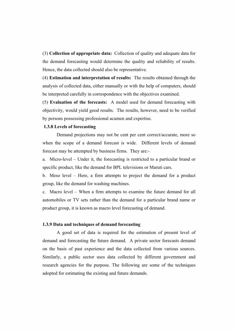
(a) Constant returns to scale: This indicates that if all factors of production are

increased in a given proportion then the output produced would also increase in

exactly the same proportion. That is, if the quantities of labour or capital or both

are increased by 10%, output would also increase by 10%. This is illustrated by

diagram-6.

Diagram 6: Constant Returns to Scale

IQ 300

IQ 200

IQ 100A

B

C

E

L

K

0

The equi-distance between successive isoquants along the product line reflects

the phenomenon. Here, the distance OA = AB = OC on the ray from the origin

which is known as product line. It represents alternatives paths of increasing

output by increasing combinations of factor inputs L and K, regardless of their

prices.

(b) Increasing returns to scale: It indicates that when all factors are increased

in a given proportion, output increases in a greater proportion. That is, if labour

and capital are increased by 10%, output increases by more than 10%.

Increasing returns to scale may occur because of expansion in the scale of

operation, and greater productive efficiency of managers and labour due to

greater specialization. This is known as economies of scale. Diagram-7

illustrates this situation.

Diagram 7: Increasing Returns to ScaleL

K

A

B

CIQ 300

IQ 200

IQ 100

D

In the diagram, the distance between successive isoquants goes on decreasing,

indicating that larger quantities of output may be produced with smaller

quantities of factor inputs. This is shown along the product line, where OA >

AB > BC.

(c) Decreasing returns to scale: It indicates that output increases in less than

proportion to the increase in factor inputs. This may be due to the scale of

operation beyond the optimum plant capacity, over-utilization of machineries

resulting in wear and tear and break-down leading to increased maintenance

cost, overworking labour, managerial constraints in over-seeing expanded

business, wastage of raw materials, etc. This is known as diseconomies of scale.

Diagram-8 shows this.

K

L

A

B

CF

IQ 300

IQ 200

IQ 100

Diagram 8: Decreasing Returns to Scale0

The diagram shows that the distance between the successive isoquants along the

product line goes on increasing, due to increased input requirements resulting

from diseconomies of scale. That is, OA < AB < BC.

1.5 Cost Concepts

A cost function expresses the relationship between the cost of production

and levels of output. The various cost concepts are:-

(1) Social and private costs: Social cost of producing a commodity refers to the

opportunities of producing other commodities foregone, given the scarce

resources. In simple terms, it is the cost of alternative good sacrificed by a

community in producing a certain amount of one good. Private costs, on the

other hand, include the costs incurred by an individual firm to obtain the

resources used for the production of commodity. The reduction in private cost of

a product would result in the reduction in of social cost, due to the emergence of

a divergence between the social and private motives.

(2) Explicit and implicit costs: Production of a commodity generally requires

different kinds of labour and capital in many forms. Modern economists call

the direct production expenses as the explicit costs of production. It includes the

expenses incurred by a producer on buying the productive services owned by

others. Whereas, implicit costs include the evaluation of a producer’s efforts and

sacrifices incurred in production process. In other words, it refers to the reward

a producer would like to pay self for self-owned and self-employed resources.

They include a normal return on own investment, and the opportunity cost

(alternative earnings) of own labour.

(3) Economic versus accounting costs: Accounting cost includes the expenses

incurred on production process, in addition to the wear and tear of machines and

equipments, which can be translated into monetary terms. The accountant

records all the explicit costs in the account book, so as to compare them with the

sale proceeds in order to compute profits. Whereas, economic cost includes all

the implicit and explicit costs of production. It involves the estimation of

opportunity cost, which is the price a factor of production can receive in any

alternative use, including the implicit costs of the factors owned by the

entrepreneur.

(4) Sunk costs: They are the costs which cannot be recovered, and therefore, are

not included in the decision making process. They include the costs of highly

specialized resources or inputs, which once installed, cannot be put to any

alternative use. For e.g., a big plant or machine installed by a firm which has

become obsolete or inoperative due to non-availability of some parts, then the

money spent on it is known as a sunk cost. It is sunk because neither can the

firm uses it, nor sell it, or put it to any alternative use. Hence, sunk costs have

no relevance in decision making.

(5) Fixed and variable costs: In production process, some factors are constant

in the short run, while others are variable. Fixed costs are costs which do not

vary with a change in output. The examples are interest on capital, rent on

building, salaries to the staff, etc., which must be incurred, regardless of the

level of output. On the other hand, variable costs change with the variations in

the level of output. They include the payments made to the variable factors,

such as wages paid to workers, raw materials, electricity, transportation cost,

etc.,

Total cost is the sum total of fixed and variable costs.

Total Cost = Fixed Costs + Variable Costs

or TC = FC + VC

TC FC VC

ATC or Average Total Cost = = +

Q Q Q

where, Q = quantity of output produced.

Thus, average cost of production is the sum total of average fixed cost

and average variable cost.

In ordinary accounting statements generally only explicit or money costs

incurred in production process are considered. However, for a realistic

computation of costs, two additional variables must be included, viz., normal

profit and implicit costs or opportunity costs (already seen). Normal profit

refers to the returns which the owners expect to receive from the business done

by the firm, in the absence of which they would prefer to quit. When total

revenue (TR) is equal to total cost (TC), the firm earns only the expected

minimum return on the capital invested, i.e. normal profit. Hence, normal profit

is a part of the cost of production. When TR exceeds TC, the firm gets super

normal profit, which is more than what a firm needs to remain in business. But

when TR = TC, the firm earns only normal profit.

1.5.1 Theory of cost in the short run

Short-run is the duration of time in which some factors of production

remain fixed, while other factors are variable. It is the time period during which

a firm cannot vary its production capacity. This capacity is determined by the

amount of fixed inputs or the size of the plant, and the costs associated with it,

which must be paid by a firm regardless of the level of output. Meanwhile, the

level of variable costs varies directly with the level of output. When returns to

variable inputs increase at an increasing rate, variable costs would increase at a

decreasing rate, and when returns to variable inputs increase at a decreasing rate,

variable costs increase at an increasing rate

Thus, while the variable cost increases directly with the level of output,

but total fixed cost remains unchanged.

Diagram-9 shows the fixed, variable and total costs.

Quantity of Output

TC

Cos

t (R

upee

s)

N

Diagram - 9 Fixed, Variable and Total Cost Curves

Q

TVC

TFC

The diagram shows that both total variable cost (TVC) and total cost

(TC) curves are increasing functions of the level of output. TVC initially

increases at a decreasing rate and then at an increasing rate. However, the total

fixed cost curve remains constant at all output levels. The shape of total cost

curve (TC) reflects that at each level of output, total cost exceeds the variable

cost. The vertical distance between TC and TVC represents total fixed cost.

Initially, the distance between TC and TVC is relatively high when the

proportion of fixed to total cost is high. But, as the level of output increases,

fixed cost constitutes a small fraction of total cost and hence the TC converges

towards TVC. This is because, with the rise in the level of output produced, the

fixed cost gets distributed across larger units of output. This reduces the fixed

cost per unit of output.

Total product and total variable cost: Logically, TVC is expected to be a strictly

increasing function of output. Further, larger levels of output generally require

greater outlays. This relationship may be expressed as follows: -

TVC = f(Q)

But, Q = g(X),

Therefore, TVC = h(X) ---- (1)

Equation (1) states that since total variable cost is a function of the level

of output (Q), the output itself is a function of the level of variable input (X).

Therefore, TVC is a function of variable input. However, as larger levels of Q

require higher amounts of variable input, with constant price of X; this

relationship can be written as follows: -

G(X1) > f (X0) if and only if X1 < X0

Hence,

H(X1) > h(X0) ---- (2)

Equation (2) indicates that TVC will increase as the level of input use

increases from X0 to X1, which in turn results in an increase in output from Q to

Q1, thus affecting TVC (Barla , 2000).

Average and marginal cost: Unit cost and the incremental cost of production

can also be computed. It has been seen that total cost of production is the sum

total of total fixed cost and total variable cost, i.e.,

TC = TFC + TVC ----- (3)

Dividing both sides of equation (3) by the quantity of output (Q) would

give average cost or unit cost of production. Therefore, average cost is the sum

total of average fixed cost and average variable cost. i.e.,

TC TFC TFC

= +

Q Q Q

or AC = AFC + AVC ------ (4)

As output increases, average fixed cost registers a decline. Average

variable cost, average total cost and marginal cost, decline initially and then

show an upward trend.

Total fixed cost divided by the quantity of output (Q) is average fixed

cost (AFC).

Section A of diagram - 10 shows that, the average fixed cost has an inverse

relationship with the quantity of output, such that as the output increases, AFC

decreases. This makes AFC a rectangular hyperbola, because total fixed cost is

divided by different levels of output. Thus,

Q.AFC = C, a constant.

That is, the area under AFC is always equal to TFC = C,

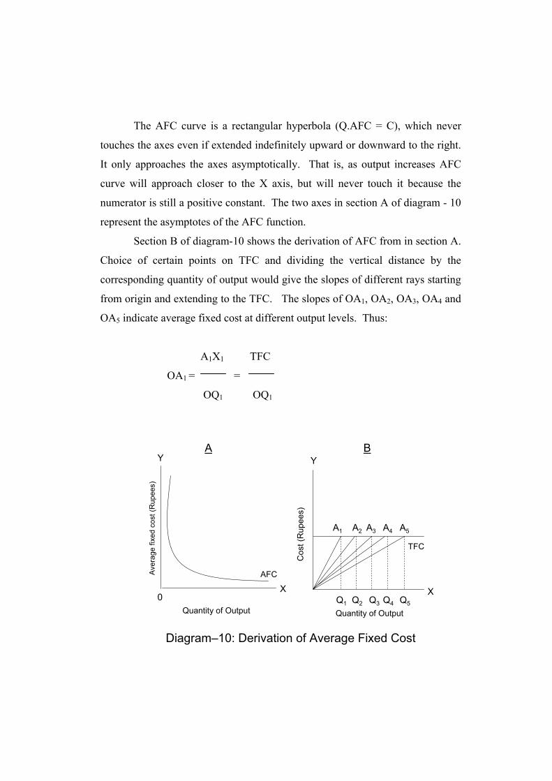
The AFC curve is a rectangular hyperbola (Q.AFC = C), which never

touches the axes even if extended indefinitely upward or downward to the right.

It only approaches the axes asymptotically. That is, as output increases AFC

curve will approach closer to the X axis, but will never touch it because the

numerator is still a positive constant. The two axes in section A of diagram - 10

represent the asymptotes of the AFC function.

Section B of diagram-10 shows the derivation of AFC from in section A.

Choice of certain points on TFC and dividing the vertical distance by the

corresponding quantity of output would give the slopes of different rays starting

from origin and extending to the TFC. The slopes of OA1, OA2, OA3, OA4 and

OA5 indicate average fixed cost at different output levels. Thus:

A1X1 TFC

OA1 = =

OQ1 OQ1

A1 A2 A3 A4 A5

Q1 Q2 Q3 Q4 Q5

Quantity of Output

Cos

t (R

upee

s)

X0

Y

Quantity of Output

TFC

Y

AFCAve

rage

fixe

d co

st (R

upee

s)

Diagram–10: Derivation of Average Fixed Cost

A B

X

It clearly shows that as OQ1 increases, the slope of OA1 declines. This

illustrates the inverse relationship between AFC and the level of output (Barla

2000).

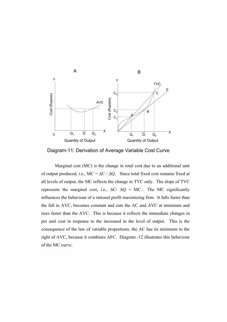
It is also possible to derive average variable cost (AVC) by measuring

the slopes of different rays from the origin to the corresponding points on the

TVC curve. However, analyzing the pattern of variation in AVC is more

complicated as compared to the AFC, because both of these elements determine

its change. Since AVC = TVC, both the numerator (TVC) and the denominator

(output) increase together, but not necessarily in the same proportion. The

traditional AVC curve is ‘U’ shaped due to the operation of law of variable

proportions. Decreasing costs arise due to economies of scale reaped by a firm,

whereas increasing costs occur due to diseconomies of scale. Section B in

diagram-11 shows TVC at different levels of output. The change in slope

indicates that TVC increases at different rates at different quantities of output.

For instance, for producing OQ1 units of output, the AVC is OC1, which is

nothing but the slope of the ray OC at A on the TVC curve.

AVC

Q1 Q Q2X

0

Y

Q1 Q Q2

CE

TVC

AB

C1

C2

C3

X

Y

A B

Quantity of OutputQuantity of Output

Cos

t (R

upee

s)

Cos

t (R

upee

s)

Diagram-11: Derivation of Average Variable Cost Curve

Marginal cost (MC) is the change in total cost due to an additional unit

of output produced, i.e., MC = ∆C / ∆Q. Since total fixed cost remains fixed at

all levels of output, the MC reflects the change in TVC only. The slope of TVC

represents the marginal cost, i.e., ∆C/ ∆Q = MC. The MC significantly

influences the behaviour of a rational profit maximizing firm. It falls faster than

the fall in AVC, becomes constant and cuts the AC and AVC at minimum and

rises faster than the AVC. This is because it reflects the immediate changes in

per unit cost in response to the increased in the level of output. This is the

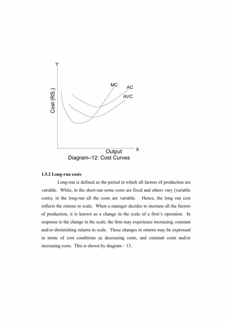
consequence of the law of variable proportions, the AC has its minimum to the

right of AVC, because it combines AFC. Diagram -12 illustrates this behaviour

of the MC curve.

Y

AC

XOutput

MC

AVC

Cos

t (R

S.)

Diagram–12: Cost Curves

1.5.2 Long-run costs

Long-run is defined as the period in which all factors of production are

variable. While, in the short-run some costs are fixed and others vary (variable

costs), in the long-run all the costs are variable. Hence, the long run cost

reflects the returns to scale. When a manager decides to increase all the factors

of production, it is known as a change in the scale of a firm’s operation. In

response to the change in the scale, the firm may experience increasing, constant

and/or diminishing returns to scale. These changes in returns may be expressed

in terms of cost conditions as decreasing costs, and constant costs and/or

increasing costs. This is shown by diagram – 13.

SAC1

SAC2

SAC3 SAC4

SAC5

SAC6

SAC7

c3c1

c2

Q1 Q2 Q3 Output0

Ave

rage

cos

t (R

s.)

Diagram-13: Long Run Cost Curves

LMC

SMC4

SMC3

SMC2

SMC1LAC

At the initial short-run average cost SAC1, the firm produces OQ1 units

of output at per unit cost OC1. When the manager plans to increase output to

OQ2 units, the average cost would be OC3 on the rising part of the SAC1 cost

curve if the same plant is used. On the other hand, if an additional plant is

installed, the cost would fall to OC2 (OC2 < OC1). Thus, the installation of a

new plant decreases the cost per unit of output. The diagram shows that average

cost will successively fall till the installation of the fourth plant. The lowest AC

level is reached at output level OQ3. This level is known as the optimum level of

output, at which the long run average cost (LAC) is minimum and the LMC cuts

it from below. Here, the long run equilibrium condition of LAC = LMC and

LMC cutting LAC from below have been reached. If output increases beyond

OQ3, the LAC would rise for every additional plants installed. No rational

manager would install new plant beyond it, as they wish to make atleast normal

profits in the long run. The long run average cost curve (LAC) is also known as

envelope curve as it envelopes several average cost curves corresponding to

different plant size. Further, it is also known as a planning curve, as it guides the

manager in planning the future expansion of plant and output.

References:

Barla C.S., Managerial Economics, National Publishing House, Raipur, 2000.

Craig Petersen H., W. Cris Lewis, Managerial Economics, Prentice-Hall of

India, New Delhi, 2003.

Dominick Salvatore, Theory and Problems of Micro Economic Theory,

Schuam’s outline series, McGraw-Hill, Inc., 1992.

Dewet K.K., Modern Economic Theory, Shyam Lal Charitable Trust, S. Chand

and Company Ltd., New Delhi, 2005.

Mote V.L., Samuel Paul and G.S. Gupta, Managerial Economics Concepts and

Cases, Tata McGraw Hill Publishing Company Ltd., New Delhi, 2001.

Koutsoyiannis. A, Modern Micro Economics, Macmillan Publishers Ltd.,

London, 1979.

Questions:

1) Distinguish between micro and macro economics.

2) Explain the concept of managerial economics.

3) List the function of a manager.

4) Illustrate the circular flow of economic activity

5) State the objectives of a firm.

6) Explain the law of demand.

7) What are the determinants of demand?

8) How is a demand curve derived?

9) Define elasticity of demand. What are its types?

10) What is demand forecasting? Discuss its stages and significance.

11) Describe the techniques of demand forecasting.

12) What is production function?

13) When is producer’s equilibrium achieved?

14) How is the law of variable proportions different from the law of returns

to scale?

15) Distinguish between economies and diseconomies of scale.

Unit – II

1. Markets

2. Classification of Markets

3. Perfect Competition

4. Monopoly

5. Price discrimination

6. Monopolistic Competition

7. Oligopoly and Duopoly

8. Wage

9. Wage Differential

OBJECTIVES

The main objectives of the chapter are:

i) To examine the features of differential market

ii) To identify price, output and profit determinants of various

forms of market

iii) To examine the reasons for wage differentials

I MARKETS

Meaning of market

A market is a place where commodities are bought and sold at retail or

wholesale prices. In economics, however, the term “market” does not refer to a

particular place as such but it refers to a market for a commodity or

commodities. Thus, the market is an arrangement whereby buyers and sellers

come in close contact with each other directly or indirectly; to sell and buy

goods is described as market. Hence, the term “market” is used in economics in

a typical and a specialized sense. They are:-

(i) It does not refer only to a fixed location. It refers to the whole area of

operation of demand and supply.

(ii) It refers to the conditions in which transactions between buyers and

sellers take place.

(iii) A group of potential sellers and potential buyers are required at different

places for creating market for a commodity.

(iv) Markets may be physically identifiable, e.g., the cutlery market in

Pondicherry situated at Jawaharlal Nehru Street.

(v) Existence of different prices for a specific commodity means existence

of different markets.

Products and factor markets

Markets may be classified into two. They are:-

(i) Product market and

(ii) Factor market.

(i) Product market

A ‘product market’ or ‘commodity market’ refers to an arrangement in

effecting buying and selling of commodities. In fact, each commodity has its

market. Thus, we speak of the cotton market, the wheat market, the rice market,

etc. Markets for precious metals such as gold and silver are called the bullion

exchanges or bullion markets. Markets for capital change such as government

securities bonds, shares, etc., are called the Stock Exchange.

(ii) Factor market.

Factor markets are markets in which factors of production such as land,

labour and capital are transacted. There are, markets called labour market, land

market, and capital market. The households or the consumers are the buyers in

the product markets. Their demand is the direct demand for the consumption

goods.

The firms or the producers are the buyers in the factor markets. Their

demand for productive resources or factors or production is a derived demand.

In the product market, the commodity price of a specific commodity is

determined individually in the concerned commodity market by the interaction

society. Factor prices such as rent of land, wages of labour and interest for

capital are determined in the factor markets as the price of each factor is

determined by the interaction between its demand and supply in its respective

market. Thus, factor markets; facilitate distribution of income in the form of

rents wages, interest and profits.

II CLASSIFICATION OF MARKETS

Classification of market structures

The market is a set of conditions in which buyers and sellers come in

contact for the purpose of exchange. The market situations vary in their

structure. Different market structures affect the behaviour of buyers and sellers.

Further, different prices and trade volumes are influenced by different market

structures. Again, all kinds of markets are not equally efficient in the

exploitation of resources, and consumers’ welfare also varies accordingly.

Hence, the different aspects of the pricing process should be analysed in relation

to the different types of markets.

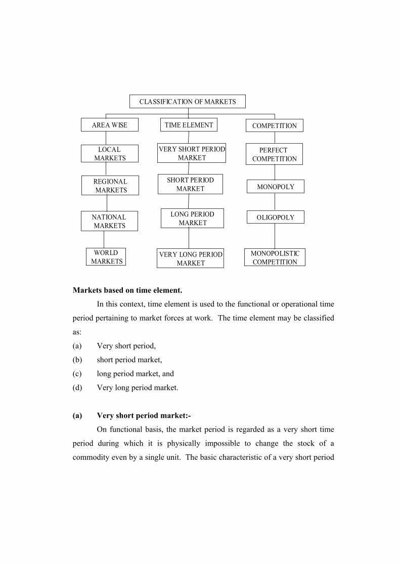
Markets may be divided on the basis of different criteria. They are:-

(i) geographical space or area,

(ii) time element and

(iii) the nature of competition.

Markets based on geographical area may be classified as:-

(a) local markets,

(b) regional markets,

(c) national markets, and

(d) world markets,

(a) Local markets:-

Markets pertaining to local areas are called local markets. When

commodities are bought and sold at one place or in one locality only, then it is

known as local markets.

(b) Regional markets:-

Goods are sold within a particular region, is known as regional market.

For example, most of the films produced in regional languages in India have

their regional markets only.

(c) National markets:-

Goods in a National market are demanded and sold on a nationwide

scale. A large number of items such as TV sets, cars, scooters, fans, vanaspati

ghee, cosmetic products, etc., produced by big companies have national markets.

A good network of transport and communication and banking facilities are

required in promoting national markets.

(d) World markets:-

In world markets goods are traded internationally. In international

markets, goods are exchanged between buyers and sellers from different

countries and we use the terms “exports” and “imports” of goods.

Classification of markets

CLASSIFICATION OF MARKETSCLASSIFICATION OF MARKETS

TIME ELEMENTTIME ELEMENT

MONOPOLISTICCOMPETITION

MONOPOLISTICCOMPETITION

VERY LONG PERIODMARKET

VERY LONG PERIODMARKET

WORLDMARKETSWORLD

MARKETS

SHORT PERIODMARKET

SHORT PERIODMARKET

LONG PERIODMARKET

LONG PERIODMARKET

VERY SHORT PERIODMARKET

VERY SHORT PERIODMARKET

PERFECT COMPETITION

PERFECT COMPETITION

AREA WISEAREA WISE COMPETITIONCOMPETITION

MONOPOLYMONOPOLY

OLIGOPOLYOLIGOPOLY

LOCAL MARKETSLOCAL

MARKETS

REGIONALMARKETS

REGIONALMARKETS

NATIONAL MARKETS

NATIONAL MARKETS

Markets based on time element.

In this context, time element is used to the functional or operational time

period pertaining to market forces at work. The time element may be classified

as:

(a) Very short period,

(b) short period market,

(c) long period market, and

(d) Very long period market.

(a) Very short period market:-

On functional basis, the market period is regarded as a very short time

period during which it is physically impossible to change the stock of a

commodity even by a single unit. The basic characteristic of a very short period

market is that in this market it is not possible to make any adjustments in the

supply to the changing demand conditions.

(b) Short period market:-

The market of a commodity during short period is referred to as “the

short period market”. During this period, it is possible for a firm to expand

output of a commodity to some extent by changing the variable inputs such as

labour, raw materials, etc., under its fixed plant size. Thus, the firm is in a

position to make some adjustment in the supply on the basis of changing

demand conditions. Besides, the equilibrium price is established by the

intersection of short period demand and short period supply.

(c) Long period market:-

The market for a commodity in the long period is referred to as “the long

period market”. Here, long period is sufficient to permit changes in the scale of

production to a firm by changing its plant size. Further, the firm is in a position

to make better period market; the equilibrium price of a commodity is

established by the interaction of long period demand and long period supply.

The price in this market is normally normal.

(d) Very long period market:-

The market for a commodity in the secular time period is referred to as

“the very long period market”. This period runs over a series of decades.

During this period, dynamic changes take place in demand and supply

conditions. There can be perfect adjustment between demand and supply in the

secular period.

Type of market structures formed by the nature of competition

Traditionally the nature of competition is adopted as the fundamental

criterion for distinguishing different types of market structure. The degree of

competition may vary among the sellers as well as the buyers in different market

situations. Usually, the market structures are classified in accordance with the

nature of competition among the sellers. The nature of competition among the

sellers is viewed on the basis of two major aspects: (1) the number of firms in

the market; and (2) the characteristics of products, such as homogeneous or

differentiated. On supply side of the market, the main types of market are:-

(i) Perfect competition,

(ii) Monopoly;

(iii) Oligopoly, and

(iv) Monopolistic competition.

III PERFECT COMPETITION

In the perfectly competitive market, a singly market price prevails for the

commodity, and it is determined by the forces of demand and supply in the

market. Under perfect competition, every participant (whether a seller or a

buyer) is a price-taker, and no one is in a position to influence it.

Characteristics of perfect competition:

The main characteristics of perfectly competitive market are:-

(a) Large number of buyers and sellers:-

A perfectly competitive market is basically formed by a large number of

actual and potential buyers and sellers. Their number is sufficiently large and the

size of each seller and buyer is relatively small in terms of market. So, the

individual seller’s buyer’s and supply and demand are negligible in terms of

market supply and demand. Hence, individual seller and buyer do not have a

control over supply and demand of the market.

(b) Homogeneous Product:-

The commodity supplied by each firm in a perfectly competitive market

is homogeneous. This means that the product of each seller is virtually

standardized. Since each firm produces an identical product, their products can

be readily substituted for each other. Hence, the buyer has no specific

preference to buy from a particular seller and his purchase from any particular

seller is a matter of chance and not of choice.

(c) Free entry and exit of firms:-

New firms are not having any legal, technological, economic, and

financial or any other barrier to their entry in the industry. Similarly, existing

firms are free to quit the market. Thus, the mobility of firms ensures that

whenever there is scope in the business, new entry will take place and

competition will remain always stiff. Due to the natural stiffness of competition,

inefficient firms would have to eventually quit the industry.

(d) Perfect knowledge of market conditions:-

Perfect competition requires that all the buyers and sellers must possess

perfect knowledge about the existing market conditions such as market price,

quantities and sources of supply and demand. The perfect knowledge ensures

transactions in a perfectly competitive market at a uniform price.

(e) Non-intervention of the Government:-

A perfect competition also implies that there is no government

intervention in the working of market economy. This means that there are no

tariffs, subsidies, rationing of goods, control on supply raw materials and

licensing policy. Government non-intervention is essential to permit free entry

of firms and for automatic adjustment of demand and supply through the market

mechanism.

(f) Absence of transport costs element.

It is essential that competitive position of no firm is adversely affected

by the transport cost differences. Hence, it is assumed that there is absence of

transport cost as all firms are closer to the markets.

Price and Output determination under perfect competition

Price for an individual firm under perfect competition is given. It cannot

influence the price by its own action. Hence, the demand curve or average

revenue curve facing a firm under perfect competition is perfectly elastic at the

ruling price. Perfectly competitive firm can sell as much as it wishes without

affecting the price, and the marginal revenue is equal to the price (average

revenue) of the commodity. So, the average revenue (or demand) curve, (AR)

and marginal revenue curve (MR) must coincide with each other for a firm

under perfect competition.

B C

X1 X

MC

A (MR = AR)P

Y

REV

ENU

E/C

OS

T

0 OUTPUT

Fig. 1 Conditions of Equilibrium Under Perfect Competition

In Fig. 1 if price prevailing in the market is OP, then PA is both the

average and marginal revenue curve. MC is the marginal cost curve. It may be

noted that under perfect competition, a firm’s upwards rising position of MC

curve is also its supply curve. Given the price OP, the firm will fix its output

where its profits are maximum. Profits are the greatest at the level of output for

which marginal cost is equal to marginal revenue and marginal cost curve cuts

the marginal revenue curve from below. In point B MC is equal to MR but MC

is cutting MR from above rather than from below. Therefore, B cannot be a

position of equilibrium. At point C or output OX1, the marginal cost equals MR

and marginal cost curve is also cutting MR curve from below. Hence, at the

output OX1, the profits would be maximum and the firm would be in

equilibrium position. Thus, the conditions of firm’s equilibrium under perfect

competition are: -

(i) MC = MR = Price

(ii) MC must cut MR from below.

Equilibrium in the Short Run

The short run has been defined as a period of time sufficient to allow the

firm to adjust its output by increasing or decreasing the amount of variable input

and fixed factors of production remains constant. Thus, in the short run, the size

and kind of plant cannot be changed, nor can new firms enter the industry.

Assume that all firms are working under identical cost conditions to

explain the equilibrium of firm under perfect competition both in the short run

and long run. The entrepreneurs of all the firms are equally efficient. Further,

let us assume that the factors of production used by the different firms are

homogeneous and are available at given and constant prices.

The above twin conditions of equilibrium ensure that profits have been

maximized or losses minimized, but they do not tell about the firm’s absolute

profit or loss position. Hence, there are three possibilities.

They are:-

(a) The firm makes supernormal profits,

(b) It makes only normal profits, and

(c) It incurs losses.

Let us explain them one by one.

(a) When the firm makes supernormal profits in the short run:-

In Fig 2, if the price is OP1, the average-marginal revenue curve is P1A1

and the firm is in equilibrium at point C1 of output OX1. The average cost is

X1G, and price is OP1. Hence, profit per unit is GC1. The output is OX1. Hence,

the firm is making supernormal profits, and it is equal to the area P1C1GH. As

all the firms in the industry have identical cost curves with the firm represented

in Fig.2, and all would be making supernormal profits. There will be a tendency

for the new firms to enter the industry and it will compete away these

supernormal profits. But the time period is not sufficient for the new firms to

enter, the industry and hence the existing firms will continue to earn

supernormal profits at the price OP1 in the short period.

SMCSAC

Q

G

A1

A

A2

QX1XQ

P2

P

P1

HF

Y

X2

R

E

S

OUTPUT

REV

ENU

E/C

OST

Fig.2 Firm’s Equilibrium: Short Run

(b) The Firm just makes normal profit:-

Let us assume that the ruling price in the market is OP. PA will then be

the average marginal revenue curve and the firm will be in equilibrium at the

point R. At the point R, besides marginal cost being equal to marginal revenue

and MC curve cutting MR curve from below, average revenue (or price) is also

equal to average cost, and the firms in the industry will be making only normal

profits which included in average cost. Since all the firms in the industry are

making only normal profits, the time period is not sufficient enough either for

the new firms to enter or for the existing firms to quit the industry.

(c) The Firm incurring Losses, but does not shutdown:-

If the short-run price in the market were OP2, instead of OP1 and OP, the

firm will be in equilibrium at point S, since with price OP2, only at S the

marginal cost is equal to marginal revenue or price OP, and MC curve cuts MR

P2A2 from below. But, at S or output OX2, the firm is incurring losses, The total

losses in this situation are equal to the area P2SEF. This is the smallest loss that

a firm can incur under the given price-cost situation, if it is to produce at all.

Given the price OP2 in the market, the loss of the firm would be greater if it tries

to produce at a point other than S.

The important question arises are:- Why at all should the firms continue

operating if they are incurring losses ? If they cannot leave the present industry,

why do they not at least shut down to avoid losses? As mentioned earlier, the

short run is a period in which firms cannot alter their fixed capital equipment.

Hence, they will have to bear fixed costs in the short run even if they shut down.

Only variable cost can be avoided by stopping production.

Shut-down point:

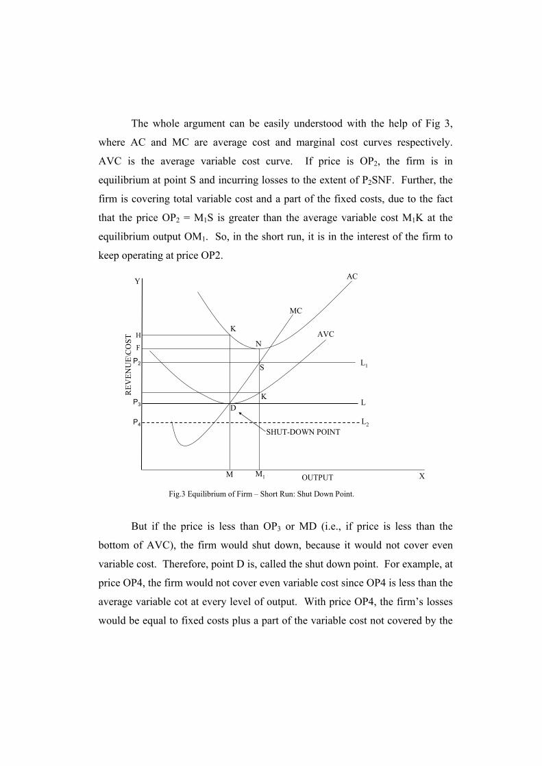
The whole argument can be easily understood with the help of Fig 3,

where AC and MC are average cost and marginal cost curves respectively.

AVC is the average variable cost curve. If price is OP2, the firm is in

equilibrium at point S and incurring losses to the extent of P2SNF. Further, the

firm is covering total variable cost and a part of the fixed costs, due to the fact

that the price OP2 = M1S is greater than the average variable cost M1K at the

equilibrium output OM1. So, in the short run, it is in the interest of the firm to

keep operating at price OP2.

L1

L

L2

D

M M1

AVC

AC

MC

Y

H

K

S

N

K

F

P2

P3

P4

X

SHUT-DOWN POINT

OUTPUT

REV

ENU

E\C

OST

Fig.3 Equilibrium of Firm – Short Run: Shut Down Point.

But if the price is less than OP3 or MD (i.e., if price is less than the

bottom of AVC), the firm would shut down, because it would not cover even

variable cost. Therefore, point D is, called the shut down point. For example, at

price OP4, the firm would not cover even variable cost since OP4 is less than the

average variable cot at every level of output. With price OP4, the firm’s losses

would be equal to fixed costs plus a part of the variable cost not covered by the

total revenue. Hence, it can be concluded that a firm will shut down if the price

falls below the bottom of average variable cost curve in the short run.

Equilibrium in the Long Run

The long run is a period which is long enough to permit changes in the

variable as well as in the fixed factors of input. Hence, firms can change their

output by increasing their fixed equipment. They can enlarge the old plants or

replace them by new plants or add new plants. Moreover, in the long run, new

firms can also enter the industry. On the contrary, if the situation so demands, in

the long run, firms can diminish their fixed equipments by allowing them to

wear out without replacement and the existing firms can leave the industry. So,

it is the long run average and marginal cost curves are relevant for making

output decisions. Further, in the long run, average cost is of no particular

relevance. It is the average total cost which is of determining importance, since

in the long run all costs are variable and none are fixed.

For a perfectly competitive firm to be in equilibrium in the long run, in

addition to marginal cost equal to price, price must also be equal to average cost.

If the price is greater than the average cost, the firms will be making

supernormal profits. Lured by these supernormal profits, new firms will enter

the industry and these extra profits will be competed away. When the new firms

enter the industry, the supply of output of the industry will increase and hence

the price of the output will be reduced. The new firms will keep coming into the

industry until the price is depressed down to average cost, and all firms are

earning only normal profits. On the other hand, if the price happens to be below

the average cost, the firms will be incurring losses. Some of the existing firms

will quit the industry. As a result, the output of the industry will decrease and

the price will rise to equal the average cost so that the firms remaining in the

industry are making normal profits. Thus the following two conditions must be

satisfied.

(i) Price = Marginal Cost

(ii) Price = Average Cost.

But if price equals both the marginal and the average costs then for the

long-run equilibrium of the firm under perfect competition, we have a combined

condition.

Price = Marginal Cost = Average Cost.

Now when average cost curve is falling, marginal cost curve is below it,

and when average cost curve is rising, marginal cost curve must be above it.

Hence, marginal cost can be equal to the average cost only at the minimum point

of average cost curve. Therefore, it is at the point of minimum average cost

curve that marginal cost curve intersects the average cost curve, and the two are

equal.

Thus, the conditions for long-run equilibrium of perfectly competitive

firm can be written as:

Price = Marginal Cost = Minimum Average Cost.

The conditions for the long-run equilibrium of the firm under perfect

competition can be easily understood from the Fig 4 where LAC is the long-run

average cost curve and LMC is the long-run marginal cost curve. The firm

under perfect competition cannot be in long-run equilibrium at price OP1

because though the price OP1 equal MC at Q but it is greater than the average

cost at this output and, therefore, the firm will be earning supernormal profits.

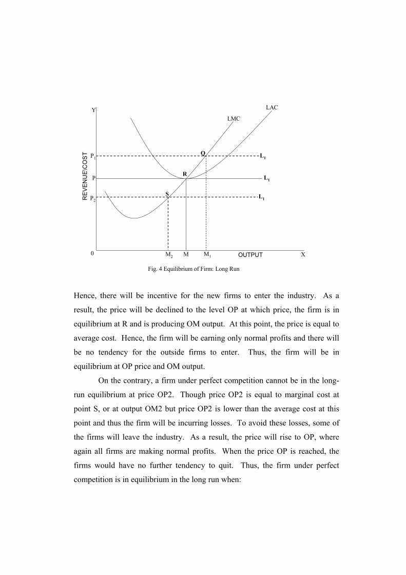
LAC

LMC

L1

L1

L1

XM1M0

P2

Y

Q

R

S

P1

P

M2 OUTPUT

RE

VEN

UE\

CO

ST

Fig. 4 Equilibrium of Firm: Long Run

Hence, there will be incentive for the new firms to enter the industry. As a

result, the price will be declined to the level OP at which price, the firm is in

equilibrium at R and is producing OM output. At this point, the price is equal to

average cost. Hence, the firm will be earning only normal profits and there will

be no tendency for the outside firms to enter. Thus, the firm will be in

equilibrium at OP price and OM output.

On the contrary, a firm under perfect competition cannot be in the long-

run equilibrium at price OP2. Though price OP2 is equal to marginal cost at

point S, or at output OM2 but price OP2 is lower than the average cost at this

point and thus the firm will be incurring losses. To avoid these losses, some of

the firms will leave the industry. As a result, the price will rise to OP, where

again all firms are making normal profits. When the price OP is reached, the

firms would have no further tendency to quit. Thus, the firm under perfect

competition is in equilibrium in the long run when:

Price = MC = Minimum AC.

An important conclusion that follows from the above discussion of

firm’s equilibrium in the long run is that the forces of competition force all the

firms to produce at the minimum point of the average cost curve. In other

words, all the firms under perfect competition tend to be of the optimum size in

the long run. This is advantageous from the viewpoint of consumers, due to the

fact that the product in question is being produced in the cheapest possible

manner without any firm incurring a loss.

Relevance of Pure Competition.

Pure competition is practically non-existence in the real world.

However, the main importances of pure competition are:-

(i) The study of the purely competitive is a rare phenomenon. But, there are

at any time in existence certain industries which resemble a competitive model.

The best example in this regard is of a contractors firm in a garment industry,

where the number of firms is large, their size and capital investment is small.

(ii) From the purely competitive model, we will be able to know how outside

forces affect an industry. Agriculture is a purely competitive industry which is

vitally affected by external factors.

(iii) The study of the purely competitive market structure is helpful in

understanding the imperfectly competitive model.

(iv) Purely competitive model is a very useful starting point for economic

analysis in the real world conditions.

(v) An understanding of a purely competitive model can enable us to study

the beneficial effects of increased production. We will be able to know, for

instance how competition lowers prices, costs and profit margins under the

impact of increased production. This is highly beneficial to the general public.

Besides, we can grasp the force of anti-trust or anti-monopoly arguments and

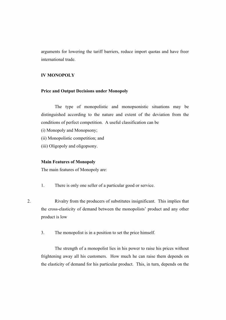
arguments for lowering the tariff barriers, reduce import quotas and have freer

international trade.

IV MONOPOLY

Price and Output Decisions under Monopoly

The type of monopolistic and monopsonistic situations may be

distinguished according to the nature and extent of the deviation from the

conditions of perfect competition. A useful classification can be

(i) Monopoly and Monopsony;

(ii) Monopolistic competition; and

(iii) Oligopoly and oligopsony.

Main Features of Monopoly

The main features of Monopoly are:

1. There is only one seller of a particular good or service.

2. Rivalry from the producers of substitutes insignificant. This implies that

the cross-elasticity of demand between the monopolists’ product and any other

product is low

3. The monopolist is in a position to set the price himself.

The strength of a monopolist lies in his power to raise his prices without

frightening away all his customers. How much he can raise them depends on

the elasticity of demand for his particular product. This, in turn, depends on the

extent to which substitutes for his products are available. And in most cases,

there is rather an infinite series of closely competing substitutes. Even exclusive

monopolies like railways or telephones must take account of potential

competition by alternative services. An undue increase in rates may lead to

substitution of railways by motor transport and of telephone calls by telegrams.

The closer the substitute and the greater the elasticity, therefore, of the demand

for a given manufacturing’s product, the less he can raise his price without

frightening away his customers. In fact, two conditions are necessary to make a

monopolist strong:

(i) A gap in the chain of substitutes, and

(ii) Possibility of securing control over all the close substitutes. In fact, it is

very difficult to draw a line between what is and what is not a monopoly.

Causes of Monopoly

Monopoly may arise due to the following reasons:

(i) The Government may grant a license to any particular person or

persons for operating public utilities like a gas company or an electricity

undertaking.

(ii) A producer may possess certain scarce raw materials, patent rights,

secret methods of production, or specialized skill which might give him

monopoly power. For example, Hoechst held a monopoly for some time in oral

medicines for diabetes because they were the first to find out the methods of

reducing blood sugar by an oral dose.

(iii) The necessity of having large resources, as is the case where the

minimum efficient scale of operations is very large, may often create monopoly.

For example, it is so for making some chemicals.

(iv) Ignorance, laziness and prejudice of the buyers may create monopoly

in favor of a particular producer.

Revenue and Costs of Monopolists

Average Revenue

If a monopolist raises his price slightly, he will sell less, but there will still be

some buyers of his product. He can increase his sales only by reducing his

price. His average revenue (demand) curve will slopes downwards to the right.

It shows that larger quantities can be sold at lower prices, whereas smaller

quantities can be sold at higher prices.

Price and Output determination under Monopoly

A firm buys competitively and sells monopolistically. It can choose to sell

many units at a lower price of fewer units at a higher price. For maximization of

profit or minimization of loss, a monopoly enterprise would curtail inputs and

outputs to the level at which the marginal revenue equals the marginal cost.

Then the slope of MC should be greater than slope of MR and and it is presented

in fig.5. In the figure equilibrium output is OQ for an equilibrium price OP.

The total revenue is OPBQ (OQ*OP) and total cost is OP0AQ (OQ*OP0).

Hence, the profit of a monopoly is P0ABP (PP0*OQ).

However, monopoly may get profit, loss or neither profit or nor loss in the short

run. But, in the long-run he will obtain only profit, otherwise he will not

continue in the firm.

MC AC

MR

AR

Em

Qm

Y

XFig 5. Price and output under Monopoly

P

P0

B

A

Disadvantages of Monopoly

The main disadvantages of Monopoly are:-

(i) When a monopolist exercises the market power by restricting

supplies, he will become richer and he will do so at the expense of those who

consume his producer.

(ii) Consumer choice is restricted because in monopoly there is only one

producer.

(iii) The absence of competition means that there will be no pressure on

the monopolist firms to be as economical as feasible. Wasteful costs tend to be

reflected in higher prices.

(iv) The exercise of monopoly power causes resources to be misallocated

from society’s point of view. As the monopolist restricts output, his output is

too small. He employs too little of society’s resources. As a result, too much of

these resources may go into the production of goods with low consumer

preferences. Thus resources are misallocated.

(v) A firm enjoying monopoly position in a strategic sector may provide

too big a risk for the economy. For example, it has been pointed out that putting

all the power engineering facilities in one company, i.e., BHEL, is full of risks,

as an natural or man-made causes of slow-down or stoppage of production

would give severe setback to the economy.

Monopsony

Monopsony is a market situation in which there is only one buyer. The main

features of monopsony are:-

1. There is only one buyer of the goods or service.

2. Rivalry from buyers who offer substitutive outlets is so remote as to be

insignificant.

3. As a result, the buyers are in a position to determine the price he pays for

the goods or services he buys.

V PRICE DISCRIMINATION

Price discrimination, also knows as differential pricing, may be defined

as the practice by a seller of charging different prices to the same buyer or to

different buyers for an individual product.

The main classes of price discrimination are:-

(i) First Degree Discrimination. The seller charges the same buyer a

different price for each unit bought. E.g., quantity discounts.

(ii) Second Degree Discrimination. The seller segregate buyers according

to income, geographic location, individual tastes, kinds of uses for the product,

and charges different prices to each group or market despite equivalent costs in

serving them. As long as the demand elasticities among different buyers are

unequal, it will be profitable for the seller to group the buyers into separates

classes according to elasticity, and charge each class a separate price.

Conditions for Price Discrimination.

The main conditions of Price discriminations are:-

(i) Multiple Demand Elasticity’s:-

There must be difference in demand elasticities among buyers due to

differences in income, location, available alternatives, tastes or other factors.

(ii) Market Segmentation:-

The seller must be able to partition (segment) the total market by

segregating buyers into groups according to elasticity.

(iii) Market sealing:-

The seller must be able to prevent, or natural circumstances must exist

which will prevent any significant resale of goods from the lower to the higher

price sub-market.

Objectives.

The objectives of price discrimination are:

(i) To appropriate the consumer’s surplus so that it accrues to the producer rather

than to the consumer.

(ii) To dispose of occasional surplus.

(iii) To develop a new market.

(iv) To make the maximum use of the unutilized capacity.

(v) To earn monopoly profits.

(vi) To enter into or retain export markets.

(vii) To destroy or to forestall competition or to make the competitors

amenable to the wishes of the seller adopting price discrimination. It may be

called predatory or discriminatory competition.

(viii) To raise future sales. This is done by quoting lower rates in the present

so that people develop in future a taste for the allied commodities produced by

the same manufacturer.

VI MONOPOLISTIC COMPETITION

Meaning and Nature:

Monopolistic competition refers to a market situation in which there are many

producers producing goods which are close substitutes of one another. The

important distinguishing characteristics of monopolistic competition are,

(a) Product Differentiation,

(b) existence of many firms supplying the market, and

(c) the goods made by them are close substitutes.

Price-output Determination under Monopolistic Competition

Under monopolistic competition, different firms, produce different

varieties of the product. Therefore, different prices for them will be determined

in the market depending upon their respective demand and cost conditions.

Each firm under monopolistic competitions seeks to achieve equilibrium or

profit-maximizing position as regards (1) price and output, (2) product

adjustment and (3) adjustment of selling costs. In other words, the producer,

under monopolistic competition, must make optimal adjustments not only in the

price charged and as regards the quantity of output sold but also in the design of

the product and the way in which he promotes the sales.

Short-run Equilibrium

In the short run, the firm will be in equilibrium when it is maximizing its

profit, i.e.,

(i) Marginal Revenue = Marginal Cost, and

(ii) Slope of marginal cost > Slope of marginal revenue.

SMC

SAC

AR

MR

XM OUTPUT0

T’

P’P

T

Y

PROFIT

CO

ST\R

EVEN

UE

Fig. 6 Equilibrium under Monopolistic Competition:Short-run

In the figures (6 and 7), AR is average revenue curve, MR is marginal

revenue curve, SAC is the short-run average cost curve, and SMC is the short-

run marginal cost curve. In these figures, marginal revenue curve (MR) and

marginal cost curve (SMC) intersects each other at the output OM at which price

is OP’.

In Fig. 6, the firm is earning supernormal profits. Supernormal profit per

unit of output is the difference between average revenue and average cost at the

equilibrium point. In this case, in equilibrium, the average revenue is MP and

average cost is MT’. Therefore, PT is the supernormal profit per unit of output.

Total supernormal profit will be measured by the area of the rectangle PTT’P’,

i.e., output multiplied by supernormal profit per unit of output.

However, if the demand and cost situation are less favorable, then the

monopolistically competitive firm will be realizing losses in the short run as

illustrated in Fig. 7. Here, the price is OP’ (=MP) which is less than the average

cost MT. TP is the loss per unit of the output OM (=PP’). Hence, the total loss

is represented by the shaded area TPP’T’. Thus, in the short run, the

monopolistically competitive firm may either realize profits or suffer losses, or

neither profit nor loss. Besides, the conditions for equilibrium under

monopolistic competition are:-

(i) MC = MR

(ii) Slope of MC > Slope of MR

SAC

SMC

ARMR

M OUTPUT X0

P

T

Y

T’

P’

LOSSES

CO

ST\R

EVEN

UE

Fig. 7 Equilibrium Under Monopolistic Competition:Short-run (with Losses)

Long-run Equilibrium of Firm and Group Equilibrium.

The firms under monopolistic competition can earn only normal profits

in the long run. This is because we assume that entry is free and new firms will

enter the industry, if the existing firms are making supernormal profits. As new

firms enter and start production, supply will increase and the price will fall, i.e.,

average revenue curve faced by the firm will shift to the left, and therefore, the

supernormal profits will be competed away and the firms will be earning only

normal profits. In, the long run, firms which are realizing losses, will leave the

industry so that the remaining firms will be earning normal profits.

Another point which is to be noted in this context is that average revenue

curve in the long run will be more elastic, due to large number of available

substitutes. Hence, in the long run, equilibrium is established when firms are

earning only normal profits. Therefore, the equilibrium in the long run under

monopolistic competition is when

Average Revenue = Average Cost.

In Fig. 8, average revenue curve (AR) is a tangent to the average cost

curve (LAC) at P. Hence, the equilibrium output in the long run is OM and the

corresponding price is MP. At this point, average cost and average revenue is

MP. Therefore, there are only the normal profits which form part of the cost of

production. Thus in the long run, the firm is in equilibrium when output is OM,

and the price is MP.

LACLMC

XM0

Y

PP

OUTPUT

REV

EN

UE

\CO

ST

Fig. 8 Equilibrium Under Monopolistic Competition:Long Run

MRAR

VII OLIGOPOLY AND DUOPOLY

But the situation in which there are two monopolists instead of one who

share the monopoly power is called Duopoly. The other is when more than two

or a few sellers are found in a monopolistic position is called Oligopoly.

Important characteristics of an oligopolistic situation are:

(a) Every seller can exercise an important influence on the price-output policies

of his rivals.

(b) Every seller is so influential that his rivals cannot ignore the likely adverse

effect on them of a given change in the price-output policy of any single

manufacturer.

(c) The rival consciousness on the part of the seller of the fact of

interdependence is the most important feature of oligopolistic situation.

(d) The demand curve under oligopoly is indeterminate, due to the fact that any

step taken by his rivals may change the demand curve.

(e) The demand curve under oligopoly are more elastic than under simply

monopoly and not perfectly elastic as under perfect competition.

DUOPOLY

Duopoly may be of two types:

(a) Duopoly without product differentiation and

(b) Duopoly with product differentiation.

Duopoly without Product Differentiation

Under duopoly the simplest cases will be those selling an identical commodity

and there is no product differentiation and there will be collusion between the

two. They may agree on a price assign quotas and divide the territory in which

each is to market his goods.

In case, if, there is no agreement between the two, a constant price war

will be the most probable consequence. The important factors to be considered

in this context will be the costs and gains in driving out the rival, the relative

sizes of the two firms, the demand elasticity and mobility of the purchasers, the

promptitude with which the rival reacts to changes in the other’s policy and the

extent to which price concession can be kept secret, and so on.

Duopoly with Product Differentiation

There is no fear of immediate retaliatory measures by the rivals. If one

producer changes his price-output policy, there is less danger of price-war. The

firm with better products can earn supernormal profits.

KINKED DEMAND CURVE

It is impossible to find a single generalized solution to the problem of

oligopoly pricing. This is because of the difficulty of knowing the exact

position of the demand curve facing a firm under oligopoly. This is turn is due

to the fact that the effect of a given price changes by a seller on the demand for

his product depends very much on the reactions of his rivals and, as we

explained earlier, rival consciousness is a basic characteristic of oligopolistic

situations.

The kinked demand curve is drawn on the assumption that the kink in the

curve is always at the ruling price. Taking the ruling price as given, it assumes

that a rise in price beyond the ruling price on the part of a given firm under

oligopoly will invite retaliation from the rivals. Otherwise, they will allow him

to raise his price and lose customers to his rivals. Hence, the upper part of the

curve is more elastic than the lower part of the curve lying below the kink. This

is because a reduction of price below the ruling price will invite immediate

retaliation from the rivals who wish to protect their own sales. The result will be

that it cannot push up its sales due to the fact that the rival firms also follow suit

with a price cut. So, the lower part of the demand curve is less elastic than the

upper one.

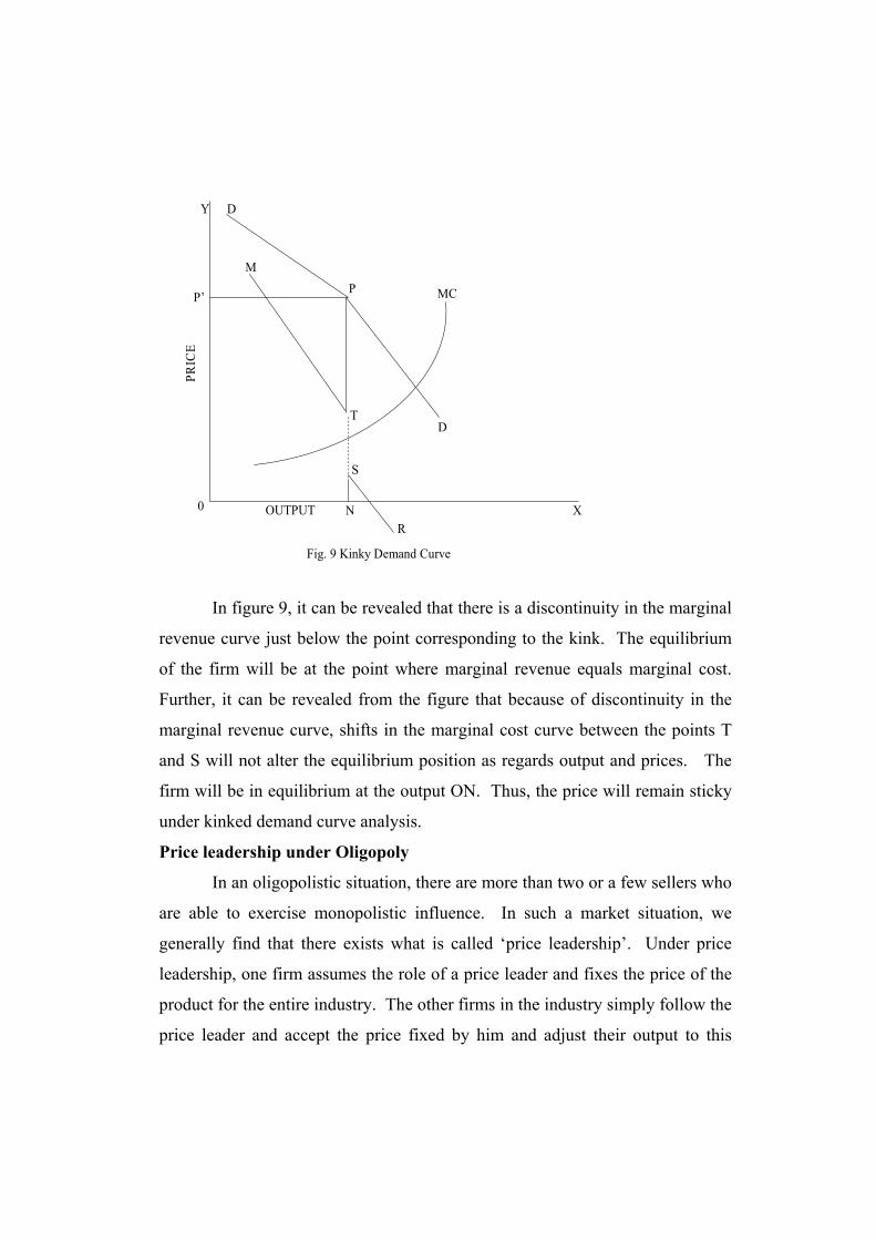
MCP

DY

P’

PRIC

E

0 NR

X

Fig. 9 Kinky Demand Curve

S

TD

M

OUTPUT

In figure 9, it can be revealed that there is a discontinuity in the marginal

revenue curve just below the point corresponding to the kink. The equilibrium

of the firm will be at the point where marginal revenue equals marginal cost.

Further, it can be revealed from the figure that because of discontinuity in the

marginal revenue curve, shifts in the marginal cost curve between the points T

and S will not alter the equilibrium position as regards output and prices. The

firm will be in equilibrium at the output ON. Thus, the price will remain sticky

under kinked demand curve analysis.

Price leadership under Oligopoly

In an oligopolistic situation, there are more than two or a few sellers who

are able to exercise monopolistic influence. In such a market situation, we

generally find that there exists what is called ‘price leadership’. Under price

leadership, one firm assumes the role of a price leader and fixes the price of the

product for the entire industry. The other firms in the industry simply follow the

price leader and accept the price fixed by him and adjust their output to this

price. The price leader is generally a very large or a dominant firm. It often

happens that price leadership is established as a result of price war in which one

firm emerges as the winner.

Types of Price Leadership

There main types of price leadership are:-

(i) Price Leadership of a Dominant Firm. Under this type of price

leadership, there is generally one firm which produces the bulk of the product of

the industry. By virtue of this position, it is able to dominate the entire market.

It sets the price and the other firms simply accept this price. The other firms are

not in a position to exercise any influence on the market price. So, the dominant

firm fixes a price so as to maximize its profits. The other firms have to adjust

their output to the price so fixed by the dominant firm.

(ii) Barometric Price Leadership. Under this type of price leadership, an

old, experienced and the largest firm assumes the role of a leader. Besides, it

protects the interests of all firms instead of merely promoting its own interest.

In a way it acts as the custodian of firms operating in the industry. It fixes a

price which is found to be suitable for all the firms in the industry. This price is

fixed by taking into consideration the market conditions with regard to the

demand for the product, cost of production, competition from the rival

producers, etc.

(iii) Exploitative or Aggressive Price Leadership. Under this category, one

big firm comes to establish its supremacy in the market by following aggressive

price policies. This firm compels other firms to follow it and accept the price

fixed by it. In case the other firms show any independence, this firm threatens

them and coerces them to follow its leadership with the result that the prices set

by this firm comes to be accepted.

Price-output Determination under Price Leadership

Economists have developed various models concerning price-output

determination under price leadership on the basis of certain assumptions

regarding the behavior of the price leader and his followers.

We take simple case here to show price-output determination under price

leadership on the following assumption:-

(a) There are only two firms X and Y and firm X has a lower cost of production

than Y,

(b) the product of the firms is homogeneous or identical so that the consumers

are indifferent as between the firms,

(c) both X and Y have equal share in the market, and they are facing the same

demand curve which will be half of the total market demand curve.

D

MCa

MCb

MRXMN

Fig. 10 Price-output Equilibrium Under Price Leadership

QUANTITY0

L

PRIC

E &

CO

ST

Y

D

KP

F

E

In figure.10, DD is the demand curve facing each firm which is half of

the total demand curve for the product, MR is the marginal cost curve of firm X

and MCY is the marginal cost curve of the firm Y. Since we have assumed that

the firm X has a lower cost of production than the firm Y, MCX is drawn below

MCY.

Let us take the firm X first, will be maximizing its profits by selling

output OM and setting price MP, because at the output OM its marginal cost is

equal to its marginal revenue. As regards the firm Y, and fixes NK price,

because at this output its marginal cost is equal to its marginal revenue. It can

be seen that the profit-maximizing price NK of the firm Y. The two firms will

have to charge the same price since the products of the two firms have been

assumed to be homogeneous. This means that the firm X, whose price MP is

lower, will dictate the price to the firm Y whose profit-making price NK is

higher. In case the firm Y refuses to fall in line, it can be ousted by the firm X

which will be charging the lower price. This shows that thus, the firm X is the

price leader and the firm Y has to follow it.

VIII WAGES

Meanings of Wages

The term, ‘wages’ means payments made for the services of labour. A

wage may be as a sum of money paid under contract by an employer to a worker

for services rendered.

Nominal Wages vs. Real Wages.

According to the classical wage theory, labour supply was considered a

function of real wages. According to Keynes, the workers acted irrationally and

generally bargained for money wages and they sharply reacted against any cut in

money wages. That is, a rise in prices does not offend labour as much as a cut in

the money wage. The money wage is also known as nominal wage. Nominal

wages are wages paid in terms of money. After deflating nominal wages with

the help of price index, we obtain real wages. The main factors influencing on

real wages are

(i) Purchasing Power of Money. When comparing wages at different

places and at different times, the changes in the purchasing power of money

must be considered. The purchasing power of money varies inversely with the

price level. This means that higher the prices, the lower the purchasing power of

money, and vice versa. It is generally supposed that the prices rise faster than

money wages during the times of rising prices and fall faster than money wages

during the periods of falling prices. The result is that money wages decline in

the former and rise in the latter case.

(ii) Subsidiary Earnings. In addition to the regular money wage, an

employee has extra earnings in the form of money or goods. For example, free

board and lodging are provided to the domestic servants. Subsidiary earnings

may also arise from opportunities of employment available to other members of

the worker’s family.

(iii) Extra Work without Extra Payment. If an employee is required to do

extra work without any compensation, his real wages are less by that extent.

Maid servants are paid for doing their duty during working hours, but quite often

they are required to work late. This means that their real earnings are reduced to

that extent.

(iv) Regularity or Irregularity of Employment. Regular employments

may give lower money wages, but the real wages may be higher than irregular

and employments which give high money wages. For instance, a person with

Rs. 50 daily wage but whose employment is intermittent, may not be so well off

as another, who earns regularly Rs. 40 day.

(iv) Conditions of Work. The conditions of work such as humanistic

approach sympathetic nature of an employer etc., should be taken into account

in estimating a person’s earnings.

(v) Future Prospects. A low money income will be considered a high real

wage if there are good prospects of a rise in the future. On the other hand, a

high initial salary may not be considered as good in the absence of prospects for

a further rise.

XI WAGE DIFFERENTIALS

In the context of wage differentials we have to explain the causes of

differences in wages in different employments and between different persons in

the same employment or grade. Wages everywhere tend to approximate to the

marginal productivity of labour. But, the marginal productivity of labour is

different in different employments and grades. It varies with the degree of

scarcity of each kind of labour in relation to the demand for it. If there were free

mobility of labour over the whole field of employment, real wage would tend to

be in proportion to the relative efficiency of labour engaged in each kind of

work. Real wage (not nominal wages) of workers of the same level of

efficiency would tend to be the same. If workers in one employment were

getting real wages more than in proportion to their efficiency, labour would tend

to move to that employment until increased supply would bring down its

marginal productivity and wages. An opposite movement would take place if in

an employment lower wages were paid than those justified by the relative

efficiency of labour.

The main causes which create differences in wages in different

employments are:-

(i) Difference in efficiency. These may be due to different inborn

qualities, education, training, and conditions under which work is performed.

Hence, wages should vary according to efficiencies.

(ii) Existence of Non-competing Groups. The non-computing groups

arise due to the difficulties in the way of mobility of labour from low-paid to

high-paid employments. These difficulties may be due to geographical, social

or economic reasons. Besides, they may arise from lack of transport facilities,

existence of family ties and caste barriers.

(iii) Difficulty of Learning a Trade. The number of those who can

master difficult trades is small. Their supply is inelastic less than demand for

them and their wages are normally will be higher.

(iv) Future Prospects. An occupation provides opportunities for future

promotion, then people will accept a lower pay, as against another occupation

offering higher initial rewards where chances of rise in future are less.

(v) Hazardous and dangerous occupations generally offer higher

emoluments.

(vi) Regularity or irregularity of employment also exerts a strong

influence on the level of wages.

(vii) Collective Bargaining. The differences in the strength and

militancy of trade unions also account for differences in wages in different

industries.

Questions:-

1) Briefly explain the market structure?

2) Distinguish between perfect competition and monopoly?

3) What are the features of perfect competition?

4) Explain how price and output is decided under perfect competition?

5) What do you mean by Shut-down point?

6) How are price and output decided under monopoly?

7) What are the features of Monopsony?

8) Explain the importance of price discrimination?

9) What are the conditions of price discrimination?

10) What are the features of monopolistic competition?

11) How are price and output decided under monopolistic competition?

12) Write short note on kinked demand curve?

13) What are the features of oligopoly?

14) Distinguish between money wage and real wage>

15) What are the determinants of real wage?

16) What are the reasons for wage differential?

17) Write short note on price leadership?

Unit – III

LESSON OUTLINE:

1. Principles of Decision Making

2. Criteria of Profit

3. Break-Even Analysis

4. Appraising Project Profitability

5. Pay-back method

6. Accounting Rate of Return

7. Internal Rate of Return

8. Net-Value Index Method

9. Probability approach for Project Appraisal

Objectives:

The main objective of the chapter is:

(i) To examine the principles of investment decision making, and

(ii) To examine the various methods of project appraisal.

Lesson 1

Principles of Decision Making

A business firm is always profit motivated. Profit seeking is the main

guiding force of any business undertaking. The classical economists have

opined that profit maximization is the sole objective of the business firm in a

capitalist economy. But, in real business, profit is not an end in itself. The

survival of the business depends on the firm’s ability to earn some profit so as to

keep the business alive.

In this context, it is worth mentioning that the reasonable profit is the

righteous reward of the entrepreneur for his entrepreneurial, organizational risk

taking activity. Hence, there is a need for rational profit policy and planning for

a modern business firm.

Most of the firms have many goals of primary importance other than

profit. Hence, the firms are interested in putting a limit on their profits. The

main reasons for limiting or controlling profits are:-

(i) Maintaining business goodwill

A policy of limiting profit may be followed by a firm in order to win

appreciation of consumers and earn business reputation and maintain business

goodwill in the market. By keeping a low profit margin, the firm may create a

good impression on the consumers and enjoy their patronage. Thus, the firm

may be in a position to maintain a stable price for its product which will

definitely fetch consumer’s appreciation by restricting profit margin an

inflationary situation.

(ii) Wage Consideration

Trade unions will demand high wages, if the firm maintains high profits

which may inflate costs and further complicate the management of business

problem. Profit control is also an important objective of running a business.

(iii) Avoiding government’s Intervention

High profits may attract high taxation. Again, high profits may be taken

as an index of monopoly power which may attract government’s attention and

investigation and its eventual control.

(iv) Minimization Risk

The risk element tends to be high under profit maximization. Hence, it is

imperative not to go in for maximization of profits but be satisfied with a

reasonable profitability of the business venture for minimizing risk.

(v) Reduction of Potential Competition

High profitability of the business may attract new competitors to enter

the field and share the market. Only a fair profit may be earned by the

concerned firm to discourage new entry in its production line.

(vi) Leadership in the Market

Firm may seek to maximize sales and capture the market rather than

maximize its profits to dominate the market and acquire leadership

(vii) Enlightened Self-interest of Survival

The firm in its own interest, for survival, would limit its profits and try to

see that its existence becomes permanent in the market so that it can earn a

regular flow of business income in the long term. It also implies considerations

to prevent loss instead of maximum return.

(viii) Liquidity Preference

In banking business greater emphasis is placed on liquidity rather than

profitability. A bank arranges its assets in the ascending order of liquidity and

descending order of profitability.

II CRITERIA FOR RATE OF PROFIT

Various criteria may be employed to determine the rate of return on

investment and decide the most acceptable rate of profit. The main criteria of

rate of profit are:-

(i) Competitive rate of profits,

(ii) Historical profit rate,

(iii) Sufficient earning to protect the equity; and

(iv) Plough back of profit rate.

(i) Competitive Rates of Profit

The firm in its profit policy may consider the guiding principle of the

rates of profits earned by other firms in the same industry.

(ii) Historical profit Rate

The firm may look into its past earnings in normal times and determine

the planned rate of return for the future course of operation.

(iii) Earning required to Protect the Equity

The rate of return on investment should adequately protect the interest of

the present shareholders, so that it has no problem in raising new equity capital

for further expansion.

(iv) Plough Back of Profit Rate

The rate of return may be such that it can adequately finance growth

through internal resources.

PROFIT ELASTICITY AND OPERATING LEVERAGE.

Profit elasticity (PE) may be defined as the ratio of proportionate change

in profit to the proportionate change in unit sales, symbolically:

% ∆π

PE = ---------

% ∆Q

or,

∆π Q

PE = ----- --- Where π = profit, and Q = unit sales.

∆Q π

Profit elasticity depends upon the following factors;

(i) Price (P)

(ii) Rate of Output (Q)

(iii) Total Fixed Cost (TFC)

(iv) Average Variable Cost (AVC)

The formula for measuring profit elasticity (PE), in this context, is:

λ

PE = ----- Where λ= Q(P-AVC), µ= TFC

λ - µ

The above mathematical formulation reveals that other thing being equal

in case of two or more firms in a business; the profit elasticity and total fixed

cost (µ) are directly related.

Example: The above point is explained by an example of three firms and it is

given below:

Profit Elasticity

Firm X Firm Y Firm Z

P= 40 P = 40 P = 40

AVC = 10 AVC = 10 AVC = 10

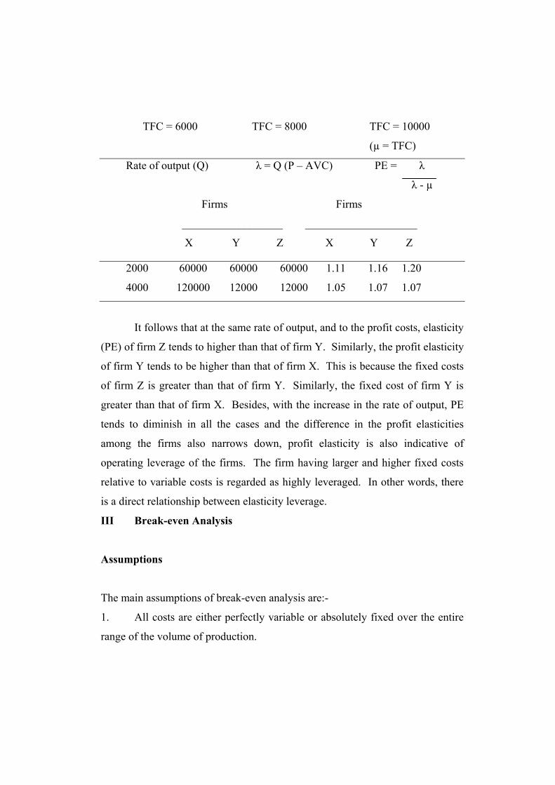
TFC = 6000 TFC = 8000 TFC = 10000

(µ = TFC)

Rate of output (Q) λ = Q (P – AVC) PE = λ

λ - µ

Firms Firms

__________________ ____________________

X Y Z X Y Z

2000 60000 60000 60000 1.11 1.16 1.20

4000 120000 12000 12000 1.05 1.07 1.07

It follows that at the same rate of output, and to the profit costs, elasticity

(PE) of firm Z tends to higher than that of firm Y. Similarly, the profit elasticity

of firm Y tends to be higher than that of firm X. This is because the fixed costs

of firm Z is greater than that of firm Y. Similarly, the fixed cost of firm Y is

greater than that of firm X. Besides, with the increase in the rate of output, PE

tends to diminish in all the cases and the difference in the profit elasticities

among the firms also narrows down, profit elasticity is also indicative of

operating leverage of the firms. The firm having larger and higher fixed costs

relative to variable costs is regarded as highly leveraged. In other words, there

is a direct relationship between elasticity leverage.

III Break-even Analysis

Assumptions

The main assumptions of break-even analysis are:-

1. All costs are either perfectly variable or absolutely fixed over the entire

range of the volume of production.

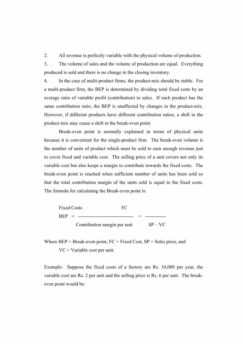
2. All revenue is perfectly variable with the physical volume of production.

3. The volume of sales and the volume of production are equal. Everything

produced is sold and there is no change in the closing inventory.

4. In the case of multi-product firms, the product-mix should be stable. For

a multi-product firm, the BEP is determined by dividing total fixed costs by an

average ratio of variable profit (contribution) to sales. If each product has the

same contribution ratio, the BEP is unaffected by changes in the product-mix.

However, if different products have different contribution ratios, a shift in the

product-mix may cause a shift in the break-even point.

Break-even point is normally explained in terms of physical units

because it is convenient for the single-product firm. The break-even volume is

the number of units of product which must be sold to earn enough revenue just

to cover fixed and variable cost. The selling price of a unit covers not only its

variable cost but also keeps a margin to contribute towards the fixed costs. The

break-even point is reached when sufficient number of units has been sold so

that the total contribution margin of the units sold is equal to the fixed costs.

The formula for calculating the Break-even point is:

Fixed Costs FC

BEP = ---------------------------------- = -------------

Contribution margin per unit SP – VC

Where BEP = Break-even point, FC = Fixed Cost, SP = Sales price, and

VC = Variable cost per unit.

Example: Suppose the fixed costs of a factory are Rs. 10,000 per year, the

variable cost are Rs. 2 per unit and the selling price is Rs. 6 per unit. The break-

even point would be:

Rs. 10,000

BEP = --------------- = 2,500 units

(6 – 2)

In other words, the company would not make any loss or profit at a sales

volume of 2,500 units and it is shown below:

Sales Rs. 15, 000

Cost of goods sold:

Variable Cost @ Rs. 2.00 Rs. 5,000

Fixed Costs Rs. 10,000 Rs. 15,000

------------ ------------

Net profit -- Nil

------------ ------------

Break-even point in terms of Sales Value.

Multi-product firms are not in a position to measure the break-even point

in terms of any common unit of product. They find it convenient to determine

their break-even point in terms of total sales in terms of monetary units. Hence,

the break-even point would be the point where the contributions margin would

be equal to the fixed costs. The contributions margin, however, is expressed as

a ratio to sales. For example, if the sales are Rs. 600 and the variable costs of

these sales is Rs. 300, the contribution margin ratio is (600 – 300 )/600, i.e., 0.5.

The formula for calculating the break-even point is:

Fixed Costs

BEP = ------------------------------

Contribution margin per unit

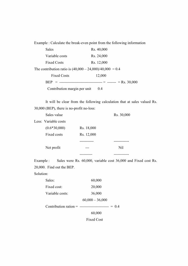
Example : Calculate the break-even point from the following information

Sales Rs. 40,000

Variable costs Rs. 24,000

Fixed Costs Rs. 12,000

The contribution ratio is (40,000 – 24,000)/40,000 = 0.4

Fixed Costs 12,000

BEP = ---------------------------------- = ------- = Rs. 30,000

Contribution margin per unit 0.4

It will be clear from the following calculation that at sales valued Rs.

30,000 (BEP), there is no-profit no-loss:

Sales value Rs. 30,000

Less: Variable costs

(0.6*30,000) Rs. 18,000

Fixed costs Rs. 12,000

----------- ------------

Net profit --- Nil

---------- ------------

Example : Sales were Rs. 60,000, variable cost 36,000 and Fixed cost Rs.

20,000. Find out the BEP.

Solution:

Sales: 60,000

Fixed cost: 20,000

Variable costs: 36,000

60,000 – 36,000

Contribution ration = ----------------------- = 0.4

60,000

Fixed Cost

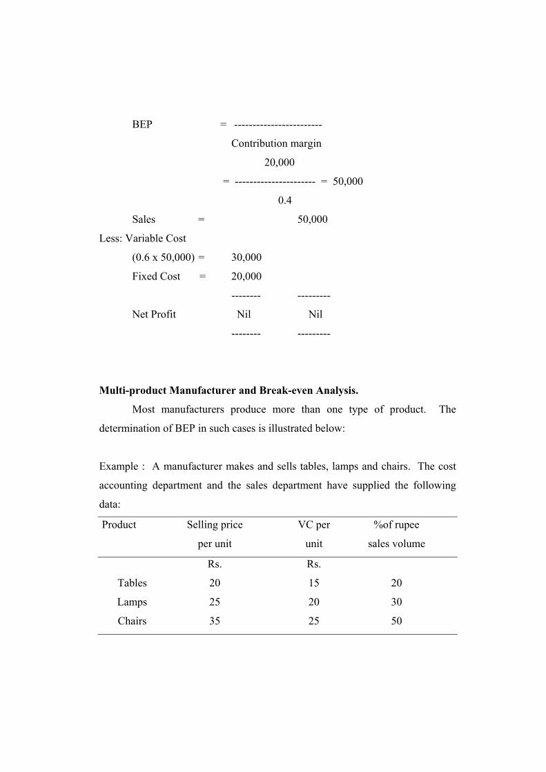
BEP = ------------------------

Contribution margin

20,000

= ---------------------- = 50,000

0.4

Sales = 50,000

Less: Variable Cost

(0.6 x 50,000) = 30,000

Fixed Cost = 20,000

-------- ---------

Net Profit Nil Nil

-------- ---------

Multi-product Manufacturer and Break-even Analysis.

Most manufacturers produce more than one type of product. The

determination of BEP in such cases is illustrated below:

Example : A manufacturer makes and sells tables, lamps and chairs. The cost

accounting department and the sales department have supplied the following

data:

Product Selling price VC per %of rupee

per unit unit sales volume

Rs. Rs.

Tables 20 15 20

Lamps 25 20 30

Chairs 35 25 50

Capacity of the firm – Rs. 3,00,000 of the total sales value.

Annual fixed cost – Rs. 20,000

Calculate (1) BEP, and (2) Profit if firm works is at 80 per cent of capacity.

Solution:

The contribution towards fixed costs in each case is:

Tables Rs. 5

Lamps Rs. 5

Chairs Rs. 10

Now, these contributions are to be converted into percentage of selling prices,

the formula being:

Selling – VC *100

Contribution percentage = -----------------------

Selling Price

Thus, the contribution percentage for individual items is:

20 – 15 1

Table – --------- x 100 = --- x 100 = 25 per cent

20 4

25 – 20 1

Lamp – --------- x 100 = --- x 100 = 20 per cent

25 5

35 – 25 1

Chair – --------- x 100 = ---- x 100 = 28.57 per cent

35 7

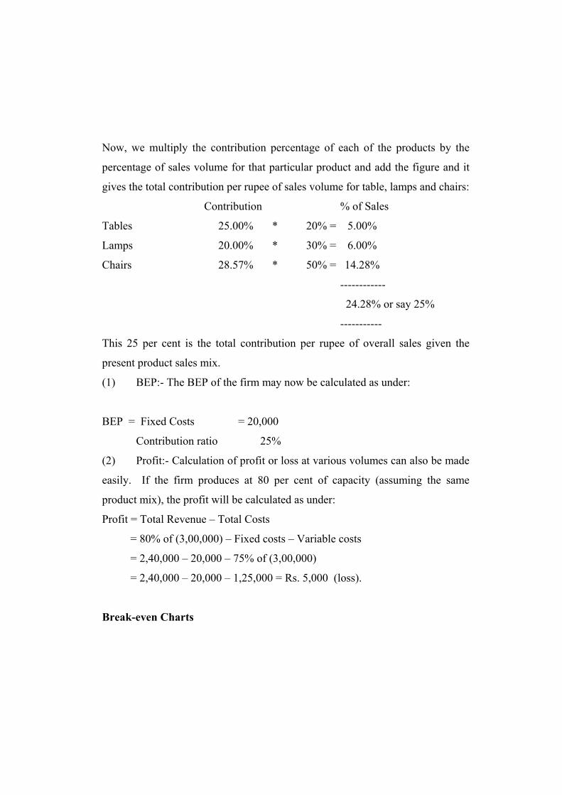
Now, we multiply the contribution percentage of each of the products by the

percentage of sales volume for that particular product and add the figure and it

gives the total contribution per rupee of sales volume for table, lamps and chairs:

Contribution % of Sales

Tables 25.00% * 20% = 5.00%

Lamps 20.00% * 30% = 6.00%

Chairs 28.57% * 50% = 14.28%

------------

24.28% or say 25%

-----------

This 25 per cent is the total contribution per rupee of overall sales given the

present product sales mix.

(1) BEP:- The BEP of the firm may now be calculated as under:

BEP = Fixed Costs = 20,000

Contribution ratio 25%

(2) Profit:- Calculation of profit or loss at various volumes can also be made

easily. If the firm produces at 80 per cent of capacity (assuming the same

product mix), the profit will be calculated as under:

Profit = Total Revenue – Total Costs

= 80% of (3,00,000) – Fixed costs – Variable costs

= 2,40,000 – 20,000 – 75% of (3,00,000)

= 2,40,000 – 20,000 – 1,25,000 = Rs. 5,000 (loss).

Break-even Charts

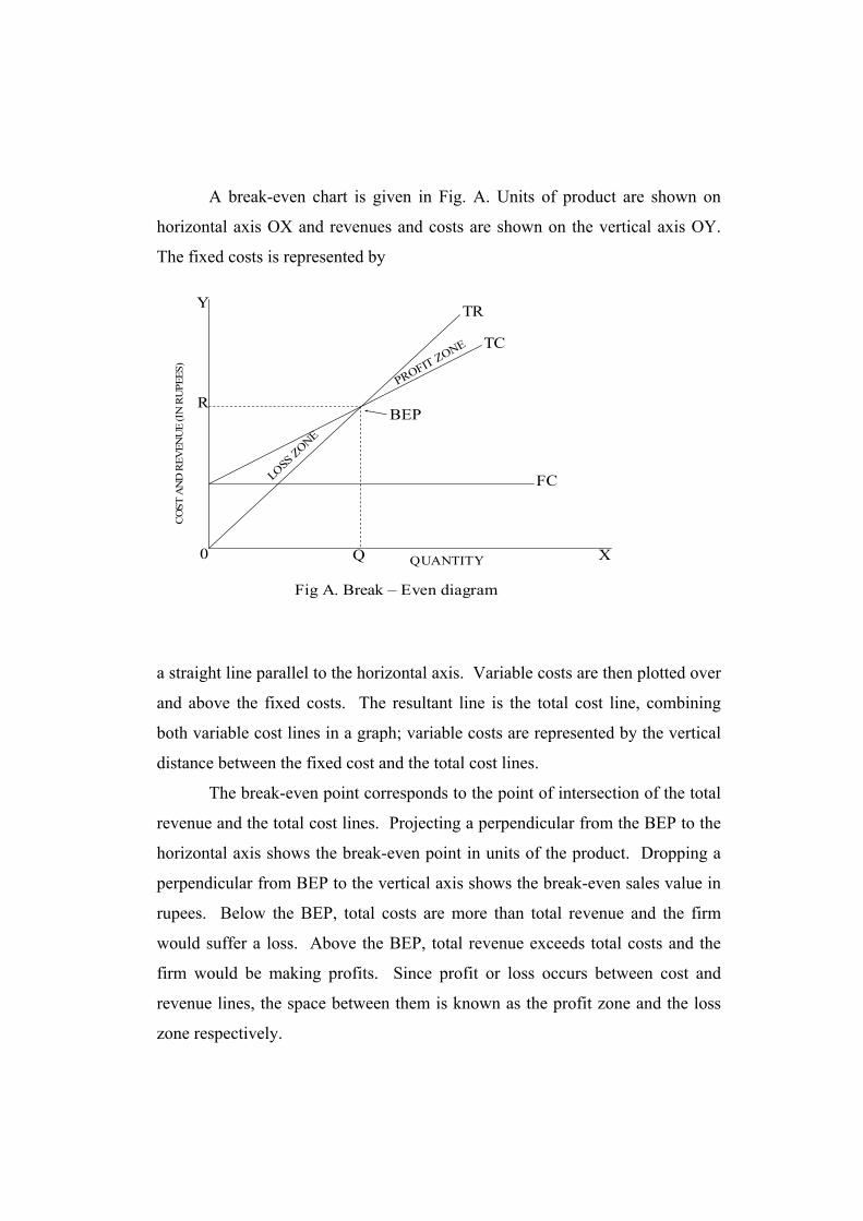
A break-even chart is given in Fig. A. Units of product are shown on

horizontal axis OX and revenues and costs are shown on the vertical axis OY.

The fixed costs is represented by

BEP

TR

TC

FC

XQ

Fig A. Break – Even diagram

0

R

CO

ST A

ND

REV

ENU

E (I

N R

UPE

ES)

Y

QUANTITY

LOSS ZONE

PROFIT ZONE

a straight line parallel to the horizontal axis. Variable costs are then plotted over

and above the fixed costs. The resultant line is the total cost line, combining

both variable cost lines in a graph; variable costs are represented by the vertical

distance between the fixed cost and the total cost lines.

The break-even point corresponds to the point of intersection of the total

revenue and the total cost lines. Projecting a perpendicular from the BEP to the

horizontal axis shows the break-even point in units of the product. Dropping a

perpendicular from BEP to the vertical axis shows the break-even sales value in

rupees. Below the BEP, total costs are more than total revenue and the firm

would suffer a loss. Above the BEP, total revenue exceeds total costs and the

firm would be making profits. Since profit or loss occurs between cost and

revenue lines, the space between them is known as the profit zone and the loss

zone respectively.

Managerial Uses of Break-even Analysis.

The main managerial uses of break-even analysis are:-

(i) It presents a microscopic picture of the profit structure of a business

enterprise.

(ii) It sharpens the focus on certain leverages which can be operated

upon to enhance its profitability.

(iii) It is possible for the management to examine the profit vulnerability

of a business firm to the possible changes in business

(iv) The analysis is immensely useful for sales prospects, changes in cost

structure, etc.

(v) It is possible to devise managerial actions to maintain and enhance

profitability of the firm.

(vi) The break-even analysis can be used for the following purposes:

(v)(a) Safety Margin: The break-even chart can help the management to know

at a glance the profits generated at the various levels of sales. The safety margin

refers to the extent to which the firm can afford a decline in sales before it starts

incurring losses. The formula for calculation of safety margin is:

(Sales – BEP) * 100

Safety Margin = ------------------------

Sales

Examples : Assume that our sales are 8,000 units and Break-even point is

6,000 units.

(8,000 – 6,000) * 100

Safety Margin = -------------------------- = 25

8,000

This means that, we can afford to lose sales up to 25 per cent of the present level

before incurring a loss. If the safety margin is dropping over a period of time, it

would mean that the firm’s resistance capacity to avoid losses has become

poorer. A margin of safety can be negative as well. In that case, it reveals the

percentage increase in sales necessary to reach the Break-even point so as to

least to avoid losses. Thus, it reveals the minimum extent of sales effort

expected of the management. Suppose in our example, sales are as low as 5,000

units. The safety margin would be:

(5,000 – 6,000) * 100

Safety Margin = --------------------------- = - 20%

5,000

In other words, the management must strive to increase sales at least by

20 per cent to avoid losses.

(v)(b) Volume Needed to Attain Target Profit. Break-even analysis may be

utilized for the purpose of determining the volume of sales necessary to achieve

a target profit. The formula is:

Fixed costs + Target profit

Target sales volume = --------------------------------

Contribution margin per unit

Example: Let desired profit is Rs. 6,000, fixed cost is Rs. 6,000 and contribution

margin is Rs. 5 per unit then the target sales volume would be calculated as

follows:

6,000 + 6,000

----------------- = 2,400 units

5

(v)(c) Change in Price. The management is often faced with a problem

whether to reduce prices or not? Before taking a decision on this question the

management will have to consider a number of points. A reduction in price

leads to a reduction in the contribution margin. This means that the volume of

sales will have to be increased even to maintain the previous level of profit. The

higher the reduction in the contribution margin, the higher is the increase in

sales needed to ensure the previous profit. The formula for determining the new

volume of sales to maintain the same profit, during the reduction in price is

given below:

FC + P

NVS = ----------

SPn – VC

Where NVS = New Volume of Sales, FC = Fixed Cost, P = Profit,

SPn = New Selling Price, and VC = Variable Cost per unit.

Example : Let Fixed cost = Rs. 10,000, Profit = Rs. 6,000, Variable cost per

unit = Rs. 2, Price reduced from Rs. 400 to Rs. 300the new sales volume needed

to maintain the previous profit of Rs. 6,000 would be

10,000 + 6,000 16,000

= ------------------ = -------- = 16,000 units

4.00 – 3.00 1.00

This would mean an increase of 11,000 units. The management can easily

decide whether this increase is feasible or not.

(v)(d) Change in Costs

A. If Variable Costs Changes. An increase in variable costs leads to a

reduction in the contribution margin. The formulae to determine the new

quantity, is given below:

(1) the new quantity will be

FC + P

NQn = ------------

SP – VCn

(2) The new selling price will be

NSP = SP + (VCn – VC) Where, NQn= New Quantity,

FC = Fixed Cost, SP= Selling Price,

NSP= New Selling Price, VC = Variable Cost, and P= Profit.

If variable cost increases from Rs. 2 to Rs. 3.50 per unit, and price is Rs. 4.00,

then

10,000 + 6,000 16,000

Qn = ------------------- = --------- = 32,000 units

4 – 3.50 0.5

Limitations

The main limitations of break-even analysis are:-

(i) A basic assumption in break-even analysis is that the cost-

revenue-volume relationship is linear and it is highly restricted.

(ii) Break-even analysis is not an effective tool for long-range use and its use

should be restricted to the short run only. The break-even analysis is limited to

the budget period of the firm normally it will be a year.

(iii) Break-even analysis assumes that profits are a function of output

ignoring the patent fact that they are also caused by other factors such as

technological change, improved management, changes in the scale of the fixed

factors of production, and so on.

(iv) A straight-line total revenue curve presumes that any quantity might be

sold at one price. This implies a horizontal demand curve and can be true only

under conditions of perfect competition. This situation is very rare in the

present world.

(v) Selling costs are difficult to handle in break-even analysis. This is due to

the fact that changes in selling costs are a cause and not a result of changes in

output and sales.

(vi) Costs in a particular period may not be caused entirely by the output in

that period. For example, maintenance expenses may be the result of past output

or a preparation for future output. So, it may, be difficult to attribute them to a

particular period.

(vii) Break-even analysis is static in character. It is based on the assumption

of given relationship between costs and revenues. Costs and revenue, may

change over time. So, making the projection based on past data is highly limited

in its use

(viii) Break-even analysis is based on accounting data, and it may suffer from

number of limitations of such data, neglect of imputed costs, arbitrary

depreciation estimates, and inappropriate allocation of overhead costs. Hence,

Break-even analysis, useful only if the firm in question maintains a good

accounting system and uses proper managerial accounting techniques and

procedures.

In view of the foregoing limitations, doubts have sometimes been raised about

the utility of break-even analysis unless it is made complex. The truth, however,

remains that break-even analysis is a device, simple, easy to understand and

inexpensive and hence quite useful to management whose primary concern is to

cut through the complexity of real world and focus attention on basic

relationships. Of course, its usefulness varies from industry to industry.

Industries suffering from frequent, volatile product-mix will not benefit much

from break-even analysis. Finally, break-even analysis should be viewed as a

guide to decision-making and not as a substitute for judgment, logical thinking

or commonsense.

IV APPRAISING PROJECT PROFITABILITY

Methods of appraising profitability

For examining the various projects under consideration, we should know

some basic information about the alternative project proposals like the initial

investment, the economic life, the scrap value, if any, the annual earnings and

the cash flow. Besides, we should consider the following factors for evaluating

a project proposal.

(i) The timing of the proceeds over the economic life of the investment

proposal, and

(ii) The duration of the proceeds: Larger the duration proceeds larger the

benefit. However, the future stream of income should be discounted

The various methods of evaluating the relative profitability of the

alternative investment projects are:

1. Pay-back Method,

2. Accounting Rate of Return,

3. Internal Rate of Return and

4. Net Present Value Index Method.

It may be noted that the pay-back period does not reveal anything about

the rates of return of different projects. The accounting Method and the Internal

Rate of return Method spells out relative rates of return of different projects.

Besides, the former method does not consider the time value of money, and the

latter consider the time value of money. Under the Net Present Value Index

Method, we proceed with our cost of capital as the base for calculating the

relative profitability of the projects. Further, the net present value method, we

also consider the time value of money.

The pay-back Method and the Accounting Method are considered as

traditional methods of investment appraisal as they are very commonly used.

The Discounted Cash Flow Method or the Internal Rate of Return and the Net

Present Value Index Method are the modern techniques as the development and

use of discounting methods is relatively new.

For purposes of illustration, we assume that there are five alternative

proposals under consideration. The details about the proposals are given in the

following table. We will examine the proposals while discussing the criteria of

project appraisal..

Proposals Initial Investment Annual Cash Flow Life in Year

Rs. Rs.

A 72,000 12,000 15

B 88,000 22,000 22

C 3,000 1,500 3

D 22,500 4,500 10

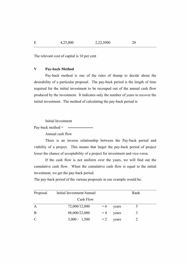
E 4,25,000 2,22,5000 20

The relevant cost of capital is 10 per cent

V Pay-back Method

Pay-back method is one of the rules of thump to decide about the

desirability of a particular proposal. The pay-back period is the length of time

required for the initial investment to be recouped out of the annual cash flow

produced by the investment. It indicates only the number of years to recover the

initial investment. The method of calculating the pay-back period is:

Initial Investment

Pay-back method = --------------------

Annual cash flow

There is an inverse relationship between the Pay-back period and

viability of a project. This means that larger the pay-back period of project

lesser the chance of acceptability of a project for investment and vice-versa.

If the cash flow is not uniform over the years, we will find out the

cumulative cash flow. When the cumulative cash flow is equal to the initial

investment, we get the pay-back period.

The pay-back period of the various proposals in our example would be:

Proposal Initial Investment/Annual Rank

Cash Flow

A 72,000/12,000 = 6 years 5

B 88,000/22,000 = 4 years 3

C 3,000 / 1,500 = 2 years 2

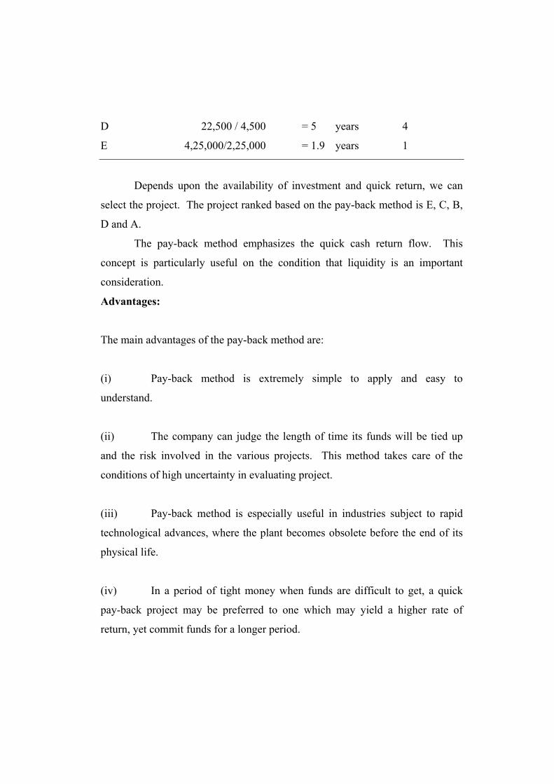
D 22,500 / 4,500 = 5 years 4

E 4,25,000/2,25,000 = 1.9 years 1

Depends upon the availability of investment and quick return, we can

select the project. The project ranked based on the pay-back method is E, C, B,

D and A.

The pay-back method emphasizes the quick cash return flow. This

concept is particularly useful on the condition that liquidity is an important

consideration.

Advantages:

The main advantages of the pay-back method are:

(i) Pay-back method is extremely simple to apply and easy to

understand.

(ii) The company can judge the length of time its funds will be tied up

and the risk involved in the various projects. This method takes care of the

conditions of high uncertainty in evaluating project.

(iii) Pay-back method is especially useful in industries subject to rapid

technological advances, where the plant becomes obsolete before the end of its

physical life.

(iv) In a period of tight money when funds are difficult to get, a quick

pay-back project may be preferred to one which may yield a higher rate of

return, yet commit funds for a longer period.

Limitations:

The main limitations of the pay-back method are:-

(i) Pay-back method over-emphasizes liquidity. Highly profitable

projects do not necessarily pay off in the initial years although large

gains may occur later.

(ii) It does little justice to a project with a long gestation period.

(iii) It also ignores long term prospects of growth.

(iv) It does not measure the rate of return.

(v) This method fails to take into account the earnings of the project after

the pay back period.

(vi) It ignores completely the time value of the money received during

and after the pay back period.

However, the pay-back method is the most widely used method for

ranking investment proposals. This is mainly due to the following reasons:

(i) In general, when the life of a project is greater than twice the pay-back

period, the reciprocal of the pay-back period is a close estimate of the

true rate of return.

(ii) Professional manager, normally employ pay-back periods as a means to

demonstrate their ability to generate a quick profit. Hence, pay-back

method is suitable to them.

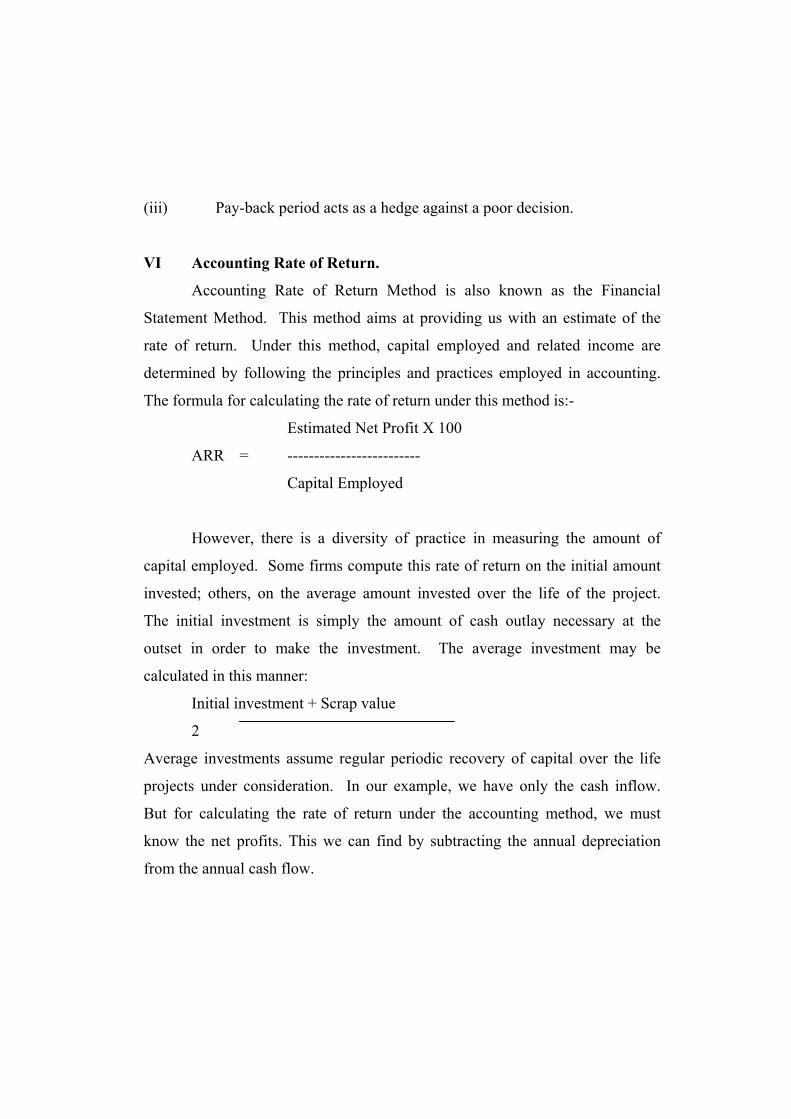
(iii) Pay-back period acts as a hedge against a poor decision.

VI Accounting Rate of Return.

Accounting Rate of Return Method is also known as the Financial

Statement Method. This method aims at providing us with an estimate of the

rate of return. Under this method, capital employed and related income are

determined by following the principles and practices employed in accounting.

The formula for calculating the rate of return under this method is:-

Estimated Net Profit X 100

ARR = -------------------------

Capital Employed

However, there is a diversity of practice in measuring the amount of

capital employed. Some firms compute this rate of return on the initial amount

invested; others, on the average amount invested over the life of the project.

The initial investment is simply the amount of cash outlay necessary at the

outset in order to make the investment. The average investment may be

calculated in this manner:

Initial investment + Scrap value

2

Average investments assume regular periodic recovery of capital over the life

projects under consideration. In our example, we have only the cash inflow.

But for calculating the rate of return under the accounting method, we must

know the net profits. This we can find by subtracting the annual depreciation

from the annual cash flow.

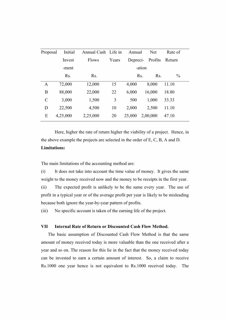
Proposal Initial Annual Cash Life in Annual Net Rate of

Invest Flows Years Depreci- Profits Return

-ment -ation

Rs. Rs. Rs. Rs. %

A 72,000 12,000 15 4,000 8,000 11.10

B 88,000 22,000 22 6,000 16,000 18.80

C 3,000 1,500 3 500 1,000 33.33

D 22,500 4,500 10 2,000 2,500 11.10

E 4,25,000 2,25,000 20 25,000 2,00,000 47.10

Here, higher the rate of return higher the viability of a project. Hence, in

the above example the projects are selected in the order of E, C, B, A and D.

Limitations:

The main limitations of the accounting method are:

(i) It does not take into account the time value of money. It gives the same

weight to the money received now and the money to be receipts in the first year.

(ii) The expected profit is unlikely to be the same every year. The use of

profit in a typical year or of the average profit per year is likely to be misleading

because both ignore the year-by-year pattern of profits.

(iii) No specific account is taken of the earning life of the project.

VII Internal Rate of Return or Discounted Cash Flow Method.

The basic assumption of Discounted Cash Flow Method is that the same

amount of money received today is more valuable than the one received after a

year and so on. The reason for this lie in the fact that the money received today

can be invested to earn a certain amount of interest. So, a claim to receive

Rs.1000 one year hence is not equivalent to Rs.1000 received today. The

present value of Rs.1000 to be received after one year is only Rs.941.8 if the rate

of interest is 6 per cent. Thus, the present value of future cash flows is less than

their face value. The later the payment is due, the lower is the present value.

This approach is neglected by the pay-back method and by the accounting

method.

The process of adjusting the face value of future cash flows to their present

value by means of an imputed interest rate is called discounting. This imputed

interest rate will be the rate of return and the rate of return calculation normally

consider, the time value of money and it is called the discounted cash flow

method.

There can be two possibilities in respect of computation of internal rate of

return they are:-

(i) The annual cash flows may be uniform over the years, and

(ii) They may be irregular or unequal.

(i) When the cash flow is uniform. The computation will involve two steps:

Initial Investment

1. Calculate the P Ratio = ----------------------

Annual Cash Flow

2. In the Present Value Table showing the present value of an annuity of

Re.1, read against the number of years of the asset’s useful life up to the interest

rate column in which the computed P ratio is located.

For example:

Proposal Initial Annual Life P Ratio Expected Rate of Return

Investment Cash flow in year

A 50,000 5,000 15 5.0 Between 15 and 20% (18.97%)

B 76,000 20,000 10 3.8 Between 25 and 30% (23.56%)

C 1,400 1,000 4 1.4 Over 40% (52.50%)

D 46,000 10,000 8 4.6 Between 15 and 20% (18.64%)

E 1,90,000 1,00,000 20 1.9 Over 40% (53.00%)

An example as to how to arrive at the rate of interest may be given here.

For proposal A, the life is 15 years. Reading against 15 years, to locate the P

Ratio, we find that the required P Ratio, of5.00 lies between 15 per cent (5.938)

and 20 per cent (4.7509). The rate can be interpolated but it would be nearer

20than 15.

The interpolation will be done by the following formula:

p – p2

r = r2 – ------- x (r2 – r1)

p1 – p2

p1 - p

or r = r1 + --------- x (r2 – r1)

p1 – p2

where p = rate of return to be determined by interpolation, r1 = lower rate of

return, r2 = higher rate of return, p1 = the P ratio at the low rate of return,

p2 = the P ratio at the higher rate of return, and v = The P ratio for which r is to

be interpolated

Applying the formula, we get

5 – 4.7509

r = 20 - ------------------- x (20 – 15)

5.9638 – 4.7509

0.2491 x 5

r = 20 - --------------- = 20 – 1.03 = 18.97

1.2129

The figures in brackets shown against the various proposals in the table

above give interpolated rates of return

For long-life projects, with constant cash flows, the pay-back reciprocal

provides a close approximation of the rate of return calculated by the discounted

cash flow method. Taking proposal A, the reciprocal of the pay-back period is

1\5 which comes to 20 per cent meaning thereby, that the approximate rate of

return on this project is 20 per cent. This is very near the rate we calculated

above.

(ii) When the Cash Flows are Unequal. Lest us assume than an

investment of Rs.1,55,000 which has a useful life of 5 years (with no scrap

value) has the following cash inflows:

1st year Rs. 30,000, 2nd year Rs. 40,000, 3rd year Rs. 60,000

4th year Rs. 50,000, 5th year Rs. 40,000

We have to calculate the rate of return through a trial-and error approach.

Accordingly, we must start by guessing at a rate interest which will discount the

future cash flows so that the total of the present values of all cash inflows proves

to be equal to the initial investment. The rate, which equates the two figures, is

the sought-for rate of return. Very often, several guesses will have to be made

before we are able to arrive at the desired rate. Let us begin with an interest rate

of 15 per cent. In this case, we have to consult Table1 which shows the present

value of Re.1 received or paid in a steady stream through out a particular year.

The present value of all cash flows comes to Rs.1,51,093 which is less than

1,55,000. This means that the rate of interest mush be less than 15 per cent.

Year Annual rate Present value Present value

factor: 15%

1 30,000 0.9286 27,858

2 40,000 0.7993 31,972

3 60,000 0.6879 41,274

4 50,000 0.5921 29,605

5 40,000 0.5096 20,384

1,51,093

Let us now try with an interest rate of 14 per cent. It will be seen that the

present value of all cash flows comes to Rs.1,54,740 which is approximation

equal to our investment. Thus we can say that the rate of return is slightly lower

than 14 per cent.

Year Annual Cash Present value Present value

flow factor: 15%

1 30,000 0.9332 27,996

2 40,000 0.8112 32,449

3 60,000 0.7050 42,318

4 50,000 0.6131 30,652

5 40,000 0.5330 21,320

1,54,737

The main merits of the internal rate of return method are:

(i) It considers the time value of money.

(ii) It considers the cash flows over the entire life of the project.

(iii) The calculation of the cost of capital is not a pre-condition for the use of

this method.

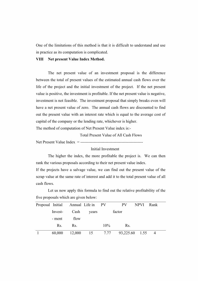
One of the limitations of this method is that it is difficult to understand and use

in practice as its computation is complicated.

VIII Net present Value Index Method.

The net present value of an investment proposal is the difference

between the total of present values of the estimated annual cash flows over the

life of the project and the initial investment of the project. If the net present

value is positive, the investment is profitable. If the net present value is negative,

investment is not feasible. The investment proposal that simply breaks even will

have a net present value of zero. The annual cash flows are discounted to find

out the present value with an interest rate which is equal to the average cost of

capital of the company or the lending rate, whichever is higher.

The method of computation of Net Present Value index is:-

Total Present Value of All Cash Flows

Net Present Value Index = -----------------------------------------------

Initial Investment

The higher the index, the more profitable the project is. We can then

rank the various proposals according to their net present value index.

If the projects have a salvage value, we can find out the present value of the

scrap value at the same rate of interest and add it to the total present value of all

cash flows.

Let us now apply this formula to find out the relative profitability of the

five proposals which are given below:

Proposal Initial Annual Life in PV PV NPVI Rank

Invest- Cash years factor

- ment flow

Rs. Rs. 10% Rs.

1 60,000 12,000 15 7.77 93,225.60 1.55 4

2 88,000 22,500 22 8.89 2,00,067.75 2.27 2

3 2,150 1,500 3 2.60 3,887.70 1.88 3

4 20,500 4,500 10 6.32 28,445.85 1.39 5

5 4,25,000 2,25,000 20 8.6466 19,45,485.00 4.58 1

There is a direct relationship between Net present value index and

acceptability of a project for investment. This means that higher the net present

value index higher the chance of acceptability of a project. Thus, in the above

example the project should be selected in the order of E, B, C, A and D.

The main merits of net present value index method are:-

(i) It considers the time value of money.

(ii) It considers the cash flows over the entire life of the project.

(iii) The calculation of the cost of capital is not a pre-condition for the use of

this method.

(iv) It avoids the problem by assuming an interest rate equivalent to the cost of

capital for finding out the present values of the cash flows. Thus, the net present

value index method has the advantage of simplicity and involves discounting of

the cash flows only once.

Other Criteria of evaluation of a project.

We have so far discussed that the projects should be ranked according to

their profitability and the various methods for finding out the relative

profitability. However, in actual business practice, managerial decisions about

investment proposals may not always be made according to their relative

profitability. There are a number of other considerations which have to be taken

into account in addition to profitability. Some of these considerations are

explained below:-

(i) Type of decision being made. The management may decide to make a

tactical decision to provide funds to a division which is making a low return to

preserve its earning power and maintain its existing market share.

(ii) Type of investment. A firm would accept a lower return on a cost

reduction programme (with relatively certain results) as against a project with a

higher but uncertain return.

(iii) Degree of certainty about cash flow. The degree of uncertainty in

relation to the estimated cash flows is an important consideration be kept in

view. Hence projects with relatively assured cash flows over with lower rates of

return are to be preferred to projects with uncertain cash flows despite high rates

of return.

(iv) Intangible factors. Very often, intangible factors such as the effect of a

course of action on company’s prestige and image. These factors cannot be

ignored and some projects may have to be accepted whether they are profitable

or not.

(v) Overall profitability. If we strictly follow the rate of return criterion, we

may be persuaded to choose a smaller investment proposal with a higher rate of

return over a large investment proposal with a lower rate of return.

(vi) Urgency of the project. Sometime, the firm may have no choice but to

make the investment irrespective of its rate of return, i.e., a roof blown by; the

cyclone should be replaced at once. Here the main point to be considered is the

cost of not doing so, i.e., the damage to merchandise and equipment which is

imminent if the roof is not immediately replaced.

IX Probability approach for Project Appraisal

We will arrive at two types of conclusions, If an experiment is repeated under

essentially homogeneous and similar conditions,. They are: - the results are

unique and the outcome can be predictable and result is not unique but may be

one of the several possible outcomes. In this context, it is better to understand

various terms pertaining to probability before examining the probability theory

pertaining to project evaluation. The main terms are explained as follows:-

(i) Random experiment:

An experiment which can be repeated under the same conditions and the

outcome cannot be predicted under any circumstances is known as random

experiment. For example: An unbiased coin is tossed. Here we are not in a

position to predict head or tail is going to occur. Hence, this type of experiment

is known as random experiment.

(ii) Sample Space

A set of possible outcomes of a random experiment is known as sample space.

For example in the case of tossing an unbiased coin twice, the possible outcomes

are HH, HT, TH and TT. This can be represented as S= ( HH, HT, TH, TT ).

(iii) An event

Any possible outcomes of a random experiment are known as an event. In the

case of tossing of an unbiased coin twice, HH is an event. An event can be

classified into two. They are: (a) Simple events, (ii) compound event. Simple

event is an event which has only one sample point in the sample space.

Compound event is an event which has more than one sample point in the

sample space. In the case of tossing of an unbiased coin twice HH is a simple

event and TH and TT are the compound events.

(iv) Complementary event

A and A’ are the complementary event if A’ consists of all those sample point

which is not included in A. For instance, an unbiased dice is thrown once. The

probability of an odd number turns up are complementary to an even number

turns up. Here, it is worth mentioning that the probability of sample space is

always is equal to one. Hence, the P(A’) = 1 - P(A).

(v) Mutually exclusive events

A and B are the two mutually exclusive events if the occurrence of A precludes

the occurrence of B. For example, in the case of tossing an unbiased coin once,

the occurrence of head precludes the occurrence of tail. Hence, head and tail are

the mutually exclusive event in the case of tossing of an unbiased coin once. If

A and B are mutually exclusive events, then the probability of occurrence of A

or B is equal to sum of their individual probabilities. Symbolically, it can be

presented as:-

P( A U B ) = P(A) + P(B)

If A and B are joint sets, then the addition theorem of probability can be stated

as:

P (A U B ) = P(A) + P(B) - P(AB)

(vi) Independent event

A and B are the two independent event if the occurrence of A does not

influence the occurrence of B. In the case of tossing an unbiased coin twice, the

occurrence of head in the first toss does not influence the occurrence of head or

tail in the second toss. Hence, these two events are called independent events.

In the case of independent event, the multiplication theorem can be stated as the

probability of A and B is the product of their individual probabilities.

Symbolically, it can be presented as:-

P(A B) = P(A) * P(B)

Addition theorem of Probability

Let A and B are the two mutually exclusive events then the probability

of A or B is equal to sum of their individual probabilities. (For detail refer

mutually exclusive events)

Multiplication theorem of Probability

Let A and B are the two independent events, then the probability of A and

B is equal to the product of their individual probabilities. ( For details refer

independent events)

Example: The odds that person X speaks the truths are 3:1 and the odds that Y

speaks the truth are 2:1. Find the probability that :-

(i) both of them speak the truth,

(ii) any one of them speak the truth, and

(iii) truth may not be told.

Solution: The probability of X speaks the truth = 1/4

The probability that X speaks lie = 3/4

The probability that Y speaks the truth = 1/3

The probability that Y speaks lie = 2/3

(i) Both of them speak truth = P(X) * P(Y)=1/4 * 1/3=1/2 (independent event)

(ii) any one of them speak truth = P(X) + P(Y) - P(X*Y)

= 1/4 + 1/3 - 1/4*1/3 = 6/12 = 1/2 ( not mutually exclusive events)

(iii) Truth may not be told = 1 – P(any one of them speak truth)

(complementary event)

= 1 – 1/2 = 1/2.

Probability distribution

Let X is discrete random variable which takes the values of x1, x2, ……….. xn

and the corresponding probabilities will be p1, p2, ……….pn. Then, X follows

the probability distribution. The two main properties of probability distribution

are :- (i) P(Xi) is always greater than or equal to zero and less than or equal to

one, and (ii) the summation of probability distribution is always equal to one.

For example tossing of an unbiased coin thrice (something needs to be added).

Then the probability of distribution is:

X ( probability of obtaining head): 0 1 2 3

P(Xi) : 1/8 3/8 3/8 1/8

Expectation of probability

Let X is discrete random variable which takes the value of x1, x2, ………… xn

then the respective probability is p1, p2, ………… pn, Then the expectation of

probability distribution is p1x1 + p2x2 + ………….. + pnxn. In the above

example, the expectation of probability distribution is

0(1/8) + 1(3/8) + 2(3/8) + 3(1/8) = 12/8 = 1.5

This indicates that on an average the probability obtaining head is 1.5 times.

Probability theory approach

A more rational method for taking into account the varying risks associated with

different investment projects is based on the probability theory. Under this

method one has to find out a range of possible cash flows, from the most

optimistic to the most pessimistic for each pertinent year, and assign

probabilities to each of the possible outcomes. The various methods of appraisal

may then be applied to each of the cash flows. Of course, the assignment of

probabilities would be subjective; depending upon each individual executive’s

beliefs and opinions. However, objectivity can be achieved by a consensus

among a team of executives or by taking an average of the probabilities assigned

by different executives to each outcome. The application of this method is

illustrated in following table

TABLE – Probability Calculation of Cash Flows

First year Second year Third year

Cash flows Proba- expec Probability Expectation Proba- Expec-

-bility tation -bility tation

Rs. Rs. Rs. Rs.

4000 0.0 - 0.0 - 0.30 1200

4500 0.0 - 0.1 450 0.30 1350

5000 0.1 500 0.1 500 0.20 1000

5500 0.2 1000 0.3 1650 0.10 550

6000 0.3 1800 0.3 1800 0.05 300

6500 0.2 1300 0.1 650 0.05 300

7000 0.1 700 0.1 700 0.0 -

7500 0.1 750 0.0 - 0.0 -

Thus, the cash flows for years 1, 2 and 3 are Rs.6050, Rs.5750, and Rs.

4725, respectively.

Questions:

1. What are the principles of decision making?

2. State the main criteria of profit

3. What are the assumptions of break-even analysis?

4. Write short note on break-even chart?

5. Explain the managerial uses of break-even analysis?

6. State the main limitations of break-even analysis

7. How for pay-back method can be used as a method of

evaluating a project proposal?

8. Write short note on accounting rate of return.

9. What are the merits and demerits of internal rate of return

method of project appraisal?

10. Explain the net present value index method by bringing out

its merits and effects?

11. critically evaluate various criteria of project evaluation.

12. Explain how uncertainty project can be evaluated?

Unit IV

Lesson Outline

I National Income

II Inflationary and Deflationary Gaps

III Economic Development

IV Technological Progress and Development

V Business and Government

Learning Objectives

After reading this lesson you should be able to understand

• The nature and scope of the concept of national income

• Models of national income determination

• Inflation and gaps

• Economic development and its indicators

• technological progress and development

• government and business enterprises

Lesson 1

National Income

Alfred Marshall defined national income (or National Dividend) as, “Labour and

capital of a country acting on its natural resources, produce annually a certain

‘net’ aggregate of commodities, material and immaterial, including services of

all kinds. The word ‘net’ means that from the gross value of the output

depreciation of capital must be deducted” According to Pigou, national income

is that part of the objective income of the community including, of course,

income derived from abroad, which can be measured in money. Prof. Fisher

based his idea of national income on consumption, rather than production. To

him, National income refers solely to services received by ultimate consumers,

whether from their material or human environment (Dewett 2005). The concept

of national income thus has three interpretations: i) receipts total, ii)

expenditure total, and iii) every expenditure is at the same time a receipt

(expenditure by one is income to another). The Keynesian concept of national

income lies between Gross National Product (G.N.P.) and Net National Product

(N.N.P.). Thus, national income of a country may be expressed in terms of three

measures:-

(a) The sum of all incomes, in cash and kind, accruing to factors of production in a

given time period, i.e., the total of income flows;

(b) The sum of net outputs arising in several sectors of the nation’s production; and

(c) The sum of consumers’ expenditure, government expenditure on goods and

services and net expenditure on capital goods.

National Income is presently defined as the aggregate factor income, arising

from the production of goods and services by a nation’s economy during a

specific period of time.

The circular flow of income may be shown using a simple two sector

model, consisting of only firms and households. Government sector and foreign

sector are ignored here, to avoid further complications arising out of their

inclusion. The economy is thus a closed economy, with no foreign trade or

external sector. Further, the model is based on the following assumptions. All

production takes place in the firms and all factors of production are owned by

the households. There is full employment. Finally, all income are spent.

Diagram-1 illustrates the real and money income flow in a two-sector model.

households firms

Commodities

expenditure on commodities

factor services

money incomeDiagram – 1 Circular flows in a two-sector economy

The firms produce goods, for which the services of factors of production are

required. The factors of production are supplied by households, for which they

receive income. With the income earned, they purchase the finished products

from the firms. This provides income to the firms, which is used for purchasing

factors of production from the households. Thus, the sales value of net

production must be equal to the sum total of payments made by the firms to the

factors of production (i.e., wages, rents, interest and profits). These incomes in

turn become the sources of expenditure of the households. Thus, income flows

from firms to households in exchange for their productive factor services, while

products flow from firms in response to the expenditure made by the

households. The flow of products in exchange for factor services is known as

the real flow, while the money income received and expenditure incurred by the

two-sector comprise the monetary flow.

The total of income flows, net outputs and final expenditures will be the same,

but the significance of each arises out of the fact that they reflect the total

operations of the nation’s economy at the level of three basic economic

functions, namely, production, distribution and expenditure.

1.1.1 Concepts of national income

There are five important concepts of national income. They are as follows:

i) Gross National Product (G.N.P.): This is the basic social accounting

measure of the total output or aggregate supply of goods and services. Gross

National Product is defined as the total market value of all final goods and

services produced in a year. The two aspects to be noted with respect to the

gross national product are:-

(a) it is a monetary measure of the market value of the output (i.e., goods and

services) produced in a year. However, to know the accurate changes in

physical output, the gross national product is adjusted for price changes by

comparing it to a base year; and

b) for the accurate computation of gross national product, the total goods and

services produced in a specific year must be accounted only once.

All finished goods go through different stages of production before being

marketed. In the process, various forms of most of the goods are purchased and

sold several times. This is likely to subject such goods to double accounting -

once in its semi-finished form, and again as the final good. In order to avoid this

problem, gross national product includes only the market values of the final

goods, and ignores the transactions of intermediate goods. Final goods are those

which are bought for final consumption and not for further processing or resale,

whereas the intermediate goods are those which are purchased for further

processing or resale. In GNP, the sales of only final goods are included and

those of the intermediate goods are excluded, because the value of final good

includes the value of intermediate goods as well. The calculation of G.N.P. also

excludes non-productive transactions, which are pure financial transactions or

transfer payments, such as old-age pensions or unemployment assistance, which

are in the nature of grants, gifts, transactions relating to existing shares, or

second-hand shares.

2) Net National Product (N.N.P.): The production process involves the use of

capital, like equipment, machinery, etc., which experience wear and tear or

depreciation in the value over time. Depreciation is known as the wear and tear

of fixed capital or fall in its value, due to its constant or continuous use during

the production process. Deducting payment for depreciation from the gross

national product constitutes net national product. N.N.P. is the market value of

all final goods and services, after deducting the depreciation charges. Hence, it

is also known as national income at market prices. That is: -

Net National Product

or

National Income at = Gross National Product + Depreciation

Market Prices

3) National Income or National Income at Factor Cost (N.I.): National

income at fixed cost differs from national income at market prices. National

income at factor cost refers to the sum total of all incomes earned by the owners

of all factors of production, resource suppliers for their contribution of land,

labour, capital, and entrepreneurial ability, during a year. Generally, it is the

national income at factor cost which is termed as ‘National Income’. The net

national product is also known as national income at market prices. The

difference between the two concepts arises from the fact that indirect taxes and

subsidies result in market prices of output, which tend to be different from the

factor incomes. For e.g., if one kg rice is sold at Rs. 20 which includes Rs. 2 of

excise and sales tax, then the market price is Rs. 20 per kg., whereas its factors

of production and distribution would receive only Rs. 18. A subsidy reduces the

market price lower than the factor cost. For e.g., if rice is subsidized at the rate

of Rs. 7 per kg and its sale price is Rs. 13, then the consumers would pay Rs.

13, whereas the factors of production and distribution would receive Rs. 20 per

kg. Thus, the value of rice at factor cost would be equal to the market price plus

the subsidies on it.

Therefore, net national product minus indirect taxes plus subsidies is

known as national income at factor cost.

National Income

or

National Income = Net National Product – Indirect Taxes +

Subsidies.

at Factor Cost

4) Personal Income (P.I.): It is the sum total of all incomes actually received by

all individuals or households during a particular year. National income is

different from personal income, because some income earned are not actually

received by households (e.g., social security contributions, corporate income

taxes and undistributed corporate profits) and some incomes received are not

currently earned (e.g., transfer payments, which include old-age pensions,

unemployment relief, other relief payments, interest payment on the public debt,

etc.). Therefore, while from national income is an indicator of income earned;

personal income is an indicator of the income actually received. Hence, these

three types of incomes which are earned but not received must be subtracted

from national income, and incomes received but not currently earned must be

added. Thus:

Personal Income = National Income – Social Security Contributions –

Corporate Income Taxes – Undistributed Corporate Profits + Transfer Payments.

5) Disposable Income (D.I.): Personal income minus the payment made to

government in the form of personal taxes, like income tax, personal property

taxes, etc., is known as disposable income. Thus,

Disposable Income = Personal Income – Personal Taxes.

This Disposable Income can be either used for consumption or saving.

Therefore, Disposable Income = Consumption + Saving.

1.1.2 National income determination models

In short-run, the level of national income is determined by aggregate demand

and aggregate supply. Supply of goods and services in a country is governed by

the productive capacity of the community, which does not change in the short-

run. However, the actual production or aggregate supply need not always be

equal to the productive capacity. But, the total output or aggregate supply will

correspond to aggregate demand. When aggregate demand rises, output will

also increase, thus raising the level of national output (i.e., national income).

Conversely, when aggregate demand decreases, the national output or national

income would also decrease, which in turn would also decrease the equilibrium

level of national income. The equilibrium level of national income is determined

by aggregate demand, as the aggregate resources of a country remain almost

constant during the short run. It is also assumed that the national output (or

income) is equal to the effective demand.

Effective demand refers to the total expenditure of the government and

the people who make expenditure on both consumption and investment goods.

Thus, effective demand consists of two components: (a) consumption demand,

i.e., demand for consumption goods, and (b) investment demand, i.e., demand

for investment goods or producers or capital goods. This may be expressed as:

Aggregate Demand = Consumption Demand + Investment Demand,

i.e., AD = C + I.

where, C = consumption demand; and I = investment demand

Consumption demand depends upon the propensity to consume (consumption

function) and income of a consumer. Given the propensity to consume, the

consumption demand increases when the increase in income. That is, there is a

positive relationship between income and consumption expenditure. Diagram-2,

shows this relationship.

Y YFX

E

E’

D F

C

C + IC + I’

Y = C + S

0

Y

Aggregate Demand

Effective Demand

Aggregate Supply

National IncomeDiagram 2: Determination of National Income

Con

sum

ptio

n an

d In

vest

men

t

G

In the diagram, the X axis represents national income and national output

(G.N.P.), and Y axis represents the consumption (C) and investment (I)

demands. A straight line of 45° from the origin represents the aggregate supply

curve. It is also called the income line. This line indicates two things: (i) total

output or aggregate supply of consumption goods and investment goods; and (ii)

national income in terms of money. Actually, the national output (G.N.P.) and

national income refer to the same thing in real and money terms respectively.

The 45° line represents equi-income-expenditure line, where the income is equal

to the expenditure.

The slope of C curve represents the propensity to consume, i.e., the change in

consumption due to a change in income. It may be observed that the C curve

starts from above the origin. It is known as the intercept or constant. It indicates

that consumption expenditure takes place even at zero income, which may be

done using past savings or borrowings. The C curve rises upwards to the right

indicating that as income increases, consumption demand also increases As the

45° line also represents national income, the distance between the curve C and

the 45° line represents saving, because a part of income after consumption is

saved. Thus,

National Income = Consumption + Saving

or, Y = C + S,

where, Y = national income, C = consumption, and S = saving.

The diagram shows the distance between the national income line Y (i.e.,

45° line ) and C ( propensity to consume) to be increasing, implying that as

income increases, the amount saved also increases. In other words, savings and

income are directly related.

The propensity to consume remains stable or constant during the short

period, because it (or the slope of curve C) depends upon the tastes and

preferences of the people, which does not change in the short run. However,

stable propensity to consume does not indicate no change in the consumption

demand. It only implies that the consumption demand which increases with an

increase in the income, does not change in the short period. Therefore, as

consumption remains more or less stable during the short run, changes in the

national income depend upon the changes in investment. Thus, investment

which is the second component of aggregate demand is an important

determinant of national income. Investment depends upon: (i) marginal

efficiency of capital, and (ii) the rate of interest. Of them, interest rate is

comparatively more stable. Therefore, the change in investment is mainly

determined by the change in marginal efficiency of capital. The marginal

efficiency of capital refers to the rate of return or expectation of profit from

investment. In other words, the expected rate of profit is known as the marginal

efficiency of capital. The marginal efficiency of capital in turn is determined by

two factors, viz., a) the replacement cost of the capital goods, and b) the

expectations of profit of the investors. Here, again, the expectations of profit are

more important determinant of investment. This implies that if a country wishes

to increase its national income or employment, then it should create an

environment wherein the profit expectations of investors and businessmen are

high.

Any time in a country, given the rate of interest and marginal efficiency

of capital, there will be a demand for investment goods. That is, entrepreneurs

would invest some amount of capital. It is assumed that investment demand

does not increase with an increase in income. On the other hand the demand for

consumption goods increases with an increase in people’s income. This in turn

raises the entrepreneur’s profit expectations, which increases the marginal

efficiency of capital, and thus results in increased investment. This clearly

indicates that the amount of investment is not directly determined by income. It

is due to this reason that diagram - 2 does not show investment demand as an

increasing function of income. Rather, it is shown combined with consumption

demand as the C+I curve.

By now it is well-known that at any given time in a country, the

entrepreneurs invest a certain amount of capital. When investment demand is

combined with the curve C, the aggregate demand curve C+1 is obtained, which

represents both consumption and investment demand. The distance between the

curve C and aggregate demand curve C+I represent investment (I). Given the

propensity to consume, higher the investment, the higher would be the aggregate

demand curve (C+I). The point at which the aggregate demand curve (C + I)

intersects the aggregate supply curve, i.e., 45° angle line, the level of national

income of a country would be determined at a given time. That is, when the

aggregate demand and aggregate supply are in equilibrium, the national income

of a country is determined at that point of time. In the diagram, the aggregate

demand curve C+I intersects the aggregate supply curve (i.e., 45° angle line) at

E. At this point, the equilibrium level of income is OY. When the income is

either more or less than OY, then the aggregate demand C+I will be more or

less, which in turn will affect the level of national income. When aggregate

demand is lower, the entire output will not be sold out. This would result in a

reduction in output, which will decrease the income. On the contrary, if income

is greater than OY, then the total output or aggregate supply will be lower than

the aggregate demand. This will lead to an increase in output, which in turn will

result in increased national income. Thus, only when income is OY, aggregate

demand and aggregate output are equal, and there will be no tendency for output

or income to decrease or increase. This is the equilibrium level of income, which

is determined by the interaction of aggregate demand and aggregate supply. At

this level, the equilibrium level of employment is also determined, because

national income, output and employment are interchangeable terms.

1.1.3 Equilibrium and full employment

It is not necessary that the equilibrium level of national income achieved

is also the point of full employment. The classicists totally opposed this view of

Keynes. The classical economists claimed that the economy would always

reach the state of full employment. Any deviation from full employment is

strictly temporary and that there is a continuous tendency in the economic

system to revert to the state of full employment. Keynes completely

contradicted this view and proved both theoretically and in reality the possibility

of under-employment equilibrium.

In the diagram - 2, assume that OYF is the full employment level of

national income. But given OY as the equilibrium level of income, it turns out

to be lower than OYF, which is the full employment level. This indicates that

the equilibrium level of income OY is at less than full employment. The

equilibrium can be achieved at full employment income, only when the saving

gap between income and consumption corresponding to full employment filled.

At OYF level of full employment income, the saving is equal to FE’. When

investment demand rises and covers this level of saving, the equilibrium level of

income will be at full employment. However, there is no guarantee that the

investment demand will be equal to saving at the full employment level of

income. This is because saving and investment are done by different sets of

people. Moreover, the factors that determine saving and investment are

different from each other. Savings are made for various purposes, like

education, construction of house, marriage, old age, future contingencies, etc.

Investment is determined by the marginal efficiency of capital and rate of

interest. Therefore, investment need not necessarily be equal to saving always at

the full employment level of national income. When investment is less than

saving, the equilibrium will be established at less than full employment.

1.1.4 Equilibrium income at equality of saving and investment

It has already been seen that the equilibrium level of national income is

achieved at the point where aggregate demand is equal to aggregate supply. The

determination of national income may also be done using the alternative method

of explaining it directly by saving and investment concepts. In diagram - 2, at

OY equilibrium level of national income, saving and investment are equal to

DE. At an income more than OY (with the aggregate demand curve C+I), the

amount of saving exceeds investment by GE’, while for income less than OY,

investment exceeds saving. This indicates that if saving and investment are not

equal, then the national income will not be in equilibrium. This is because when

at a certain level of national income the intended investment by entrepreneurs

exceeds the intended savings by people, it would indicate that aggregate demand

is greater than the aggregate supply. This would encourage firms to increase

production, which would raise the levels of employment and income. This in

turn would increase national output and thus the national income as well. Thus,

when investment is greater than saving, there will be a tendency for the national

income to increase. On the other hand, when saving is higher than investment, it

would indicate that aggregate demand is short of aggregate supply. This implies

that the entrepreneurs are unable to sell their complete output at the prevailing

price. This would lead to a decline in output, which would result in a fall in the

national income. Therefore, at a given level of national income when the

investment demand of entrepreneurs is lower than the intended savings of the

people, the national income would decrease. It will decline to the level at which

investment expenditure becomes equal to the planned savings of the community.

But, when the intended saving of the people is equal to the investment demand

at a given national income, the aggregate demand would be equal to the total

output or aggregate supply. This would result in equilibrium national income.

The determination of national income by saving and investment can

again be interpreted in yet another way. While saving comprises withdrawal of

money from the income stream, investment constitutes an injection of money

into it. When intended investment exceeds the intended saving, it would imply

that more money has been injected into the income stream than what has been

withdrawn. This would imply that the national income has increased.

Meanwhile, when investment falls short of the intended saving, it would mean

that less money has been injected into the income stream and more has been

withdrawn. As a result, the national income would decrease. On the other hand,

when investment equals saving, it would imply that the amount of money

injected has been withdrawn from the income stream. As a consequence, the

national income would neither increase nor decrease, indicating an equilibrium

condition. Thus, the equilibrium national income would be established at the

level at which the intended investment equals the intended saving.

Diagram – 3 shows the determination of national income by investment

and saving.

S

S

0

Y

XY

E II

Diagram 3: Determination of National Income by Saving and Investment

Income

Sav

ing

/ Inv

estm

ent

In the diagram, the X-axis represents income and the Y-axis represents

saving and investment. The SS curve shows intended saving and the II curve

shows the intended investment or investment demand. The SS curve is upward

sloping, indicating the intended saving to be rising at different levels of income.

The II investment curve is parallel to the X-axis, due to the assumptions that

investment does not change with income, and that entrepreneurs intend to invest

only a certain amount of money in a particular year. The SS and II curves

intersect each other at E, showing the equality between intended investment and

saving at OY level of income. This indicates that OY is the equilibrium level of

income. When the level of income is lower than OY, the amount of intended

investment exceeds the intended saving, due to which the level of income would

rise. On the other hand, when the level of income is greater than OY, the

intended saving exceeds intended investment, as a result of which the level of

income would fall. The decline in income would continue until it becomes

equal to OY. At the OY level of income, there is neither a tendency for income

to rise nor to fall, because at this level both the intended investment and

intended saving are equal. Therefore, the equilibrium level of national income is

determined by the equality in investment and saving at OY.

In sum, the equilibrium level of national income would be determined

under the fulfillment of the following two conditions:

(i) Aggregate Demand = Aggregate Supply, and

(ii) Intended Investment = Intended Saving.

Thus, the equality between aggregate demand and aggregate supply and the

equality between the intended investment and saving mean the same thing.

1.1.5 Keynesian theory of employment

During the “Great Depression” in the late 1920s, the validity of classical

economic theories completely collapsed as they failed to correct the

disequilibrium in the economic activities. Although the classical economists

advocated that demand created its own supply, savings were equal to

investment, full employment prevailed, business cycles were temporary in

nature and unemployment was a short term phenomenon, and that these

disturbances could be easily corrected by varying the interest rates or by

reducing the wage rate, nothing of the sort happened in 1919. Therefore, the

then American President Hoover introduced various policy measures to correct

the prevailing economic situations, all of which ended up being too little and too

late. As a result, he was forced to resign and President Roosevelt took over on

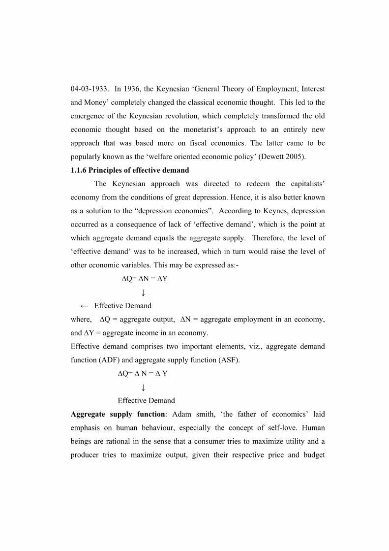
04-03-1933. In 1936, the Keynesian ‘General Theory of Employment, Interest

and Money’ completely changed the classical economic thought. This led to the

emergence of the Keynesian revolution, which completely transformed the old

economic thought based on the monetarist’s approach to an entirely new

approach that was based more on fiscal economics. The latter came to be

popularly known as the ‘welfare oriented economic policy’ (Dewett 2005).

1.1.6 Principles of effective demand

The Keynesian approach was directed to redeem the capitalists’

economy from the conditions of great depression. Hence, it is also better known

as a solution to the “depression economics”. According to Keynes, depression

occurred as a consequence of lack of ‘effective demand’, which is the point at

which aggregate demand equals the aggregate supply. Therefore, the level of

‘effective demand’ was to be increased, which in turn would raise the level of

other economic variables. This may be expressed as:-

∆Q= ∆N = ∆Y

↓

← Effective Demand

where, ∆Q = aggregate output, ∆N = aggregate employment in an economy,

and ∆Y = aggregate income in an economy.

Effective demand comprises two important elements, viz., aggregate demand

function (ADF) and aggregate supply function (ASF).

∆Q= ∆ N = ∆ Y

↓

Effective Demand

Aggregate supply function: Adam smith, ‘the father of economics’ laid

emphasis on human behaviour, especially the concept of self-love. Human

beings are rational in the sense that a consumer tries to maximize utility and a

producer tries to maximize output, given their respective price and budget

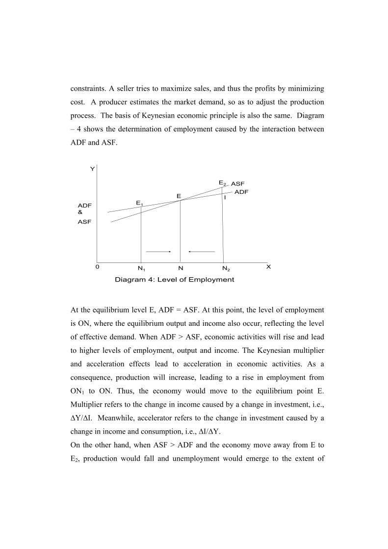
constraints. A seller tries to maximize sales, and thus the profits by minimizing

cost. A producer estimates the market demand, so as to adjust the production

process. The basis of Keynesian economic principle is also the same. Diagram

– 4 shows the determination of employment caused by the interaction between

ADF and ASF.

0

ADF &

ASF

I

Y

X

ADFE

N N2N1

E1

E2 ASF

Diagram 4: Level of Employment

At the equilibrium level E, ADF = ASF. At this point, the level of employment

is ON, where the equilibrium output and income also occur, reflecting the level

of effective demand. When ADF > ASF, economic activities will rise and lead

to higher levels of employment, output and income. The Keynesian multiplier

and acceleration effects lead to acceleration in economic activities. As a

consequence, production will increase, leading to a rise in employment from

ON1 to ON. Thus, the economy would move to the equilibrium point E.

Multiplier refers to the change in income caused by a change in investment, i.e.,

∆Y/∆I. Meanwhile, accelerator refers to the change in investment caused by a

change in income and consumption, i.e., ∆I/∆Y.

On the other hand, when ASF > ADF and the economy move away from E to

E2, production would fall and unemployment would emerge to the extent of

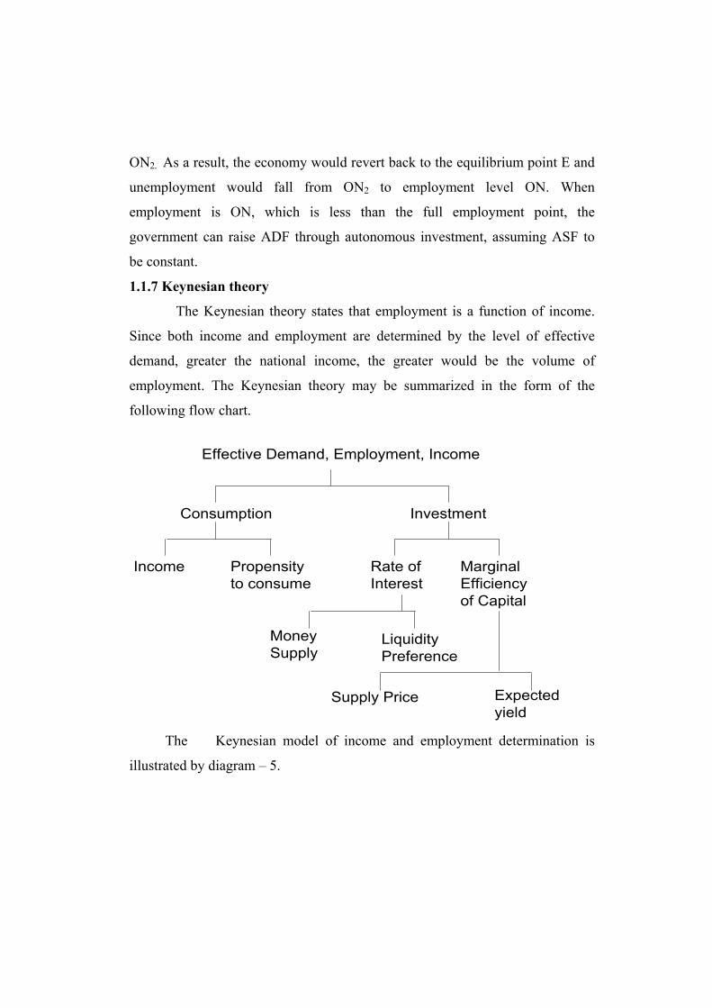
ON2. As a result, the economy would revert back to the equilibrium point E and

unemployment would fall from ON2 to employment level ON. When

employment is ON, which is less than the full employment point, the

government can raise ADF through autonomous investment, assuming ASF to

be constant.

1.1.7 Keynesian theory

The Keynesian theory states that employment is a function of income.

Since both income and employment are determined by the level of effective

demand, greater the national income, the greater would be the volume of

employment. The Keynesian theory may be summarized in the form of the

following flow chart.

Effective Demand, Employment, Income

Consumption Investment

Marginal Efficiency of Capital

Rate of Interest

Income Propensity to consume

Money Supply

Liquidity Preference

Supply Price Expected yield

The Keynesian model of income and employment determination is

illustrated by diagram – 5.

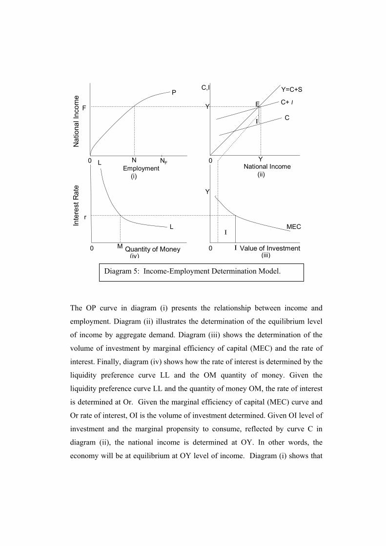
N0 L

L

Y

F

P

r

M

C

I

I0

E C+ I

Y=C+SC,I

Y

Employment National IncomeNF

(ii)(i)

Y

(iii)(iv)Quantity of Money Value of Investment0

0

Nat

iona

l Inc

ome

I

Inte

rest

Rat

e

MEC

The OP c

employme

of income

volume o

interest. F

liquidity

liquidity p

is determi

Or rate of

investmen

diagram (

economy

Diagram 5: Income-Employment Determination Model.

urve in diagram (i) presents the relationship between income and

nt. Diagram (ii) illustrates the determination of the equilibrium level

by aggregate demand. Diagram (iii) shows the determination of the

f investment by marginal efficiency of capital (MEC) and the rate of

inally, diagram (iv) shows how the rate of interest is determined by the

preference curve LL and the OM quantity of money. Given the

reference curve LL and the quantity of money OM, the rate of interest

ned at Or. Given the marginal efficiency of capital (MEC) curve and

interest, OI is the volume of investment determined. Given OI level of

t and the marginal propensity to consume, reflected by curve C in

ii), the national income is determined at OY. In other words, the

will be at equilibrium at OY level of income. Diagram (i) shows that

OY level of national income creates ON volume of employment. Assuming ONF

to be the level of full employment, the OE equilibrium represents less than full

employment level.

1.2 Inflationary and Deflationary Gaps

Inflation is the rise in price without a corresponding increase in the

supply of goods and services at a given time. In the process, the values of

commodities rise, while the value of money declines during inflation. By now it

is understood that equilibrium need not necessarily occur at the full employment

level and that it can also occur at less than full employment level. Therefore, the

equilibrium level of national income or employment has no particular feature.

For, an equilibrium level may involve both unemployment and waste of national

resources, if the investment is insufficient to ensure full employment.

Therefore, the desirable level of equilibrium is the one which is achieved at full

employment or near full employment. This level may be achieved when

investment opportunities equal full employment savings. As a result, there can

be inflationary gap or deflationary gap.

a) Inflationary gap:

When consumption and investment expenditures are greater than the full

employment GNP level, it gives rise to inflationary gap. Under this

circumstance, consumer demand for goods and services are greater than its

supply. Thus, when inflationary gap occurs, national income, output and

employment cannot increase any further. The rise in demand for goods and

services results in increased price level. In other words, inflationary gap would

occur when the scheduled investment exceeds the full employment saving.

Under such a situation, the demand for goods would be more than what the

economic system can produce. This would lead to a rise in the prices, which

would result in an inflationary situation. Thus, when the full employment

savings is lower than the scheduled investment at full employment, inflationary

gap would emerge. This situation illustrated in diagram - 6.

Inflationary Gap A E

B C+ I

C

XQQF

C+ I+ G

0

C,I,

G

Y

OutputDiagram 6: Inflationary Gap

In the diagram, C, I and, G represent consumption, investment and government

expenditures respectively. The C+I+G line represent the total expenditure in an

economy. It intersects the 45° line at E, at which the total real output is Q. QF

represents the full employment limit to real output. The real income cannot

reach Q, because at QF the total demand C+I+G exceed the total output, showing

a gap of AB. This gap AB is known as the inflationary gap in the Keynesian

sense.

b) Deflationary gap:

Deflationary gap occurs when the total aggregate demand fails to create full

employment. The Diagram - 7 shows the deflationary gap.

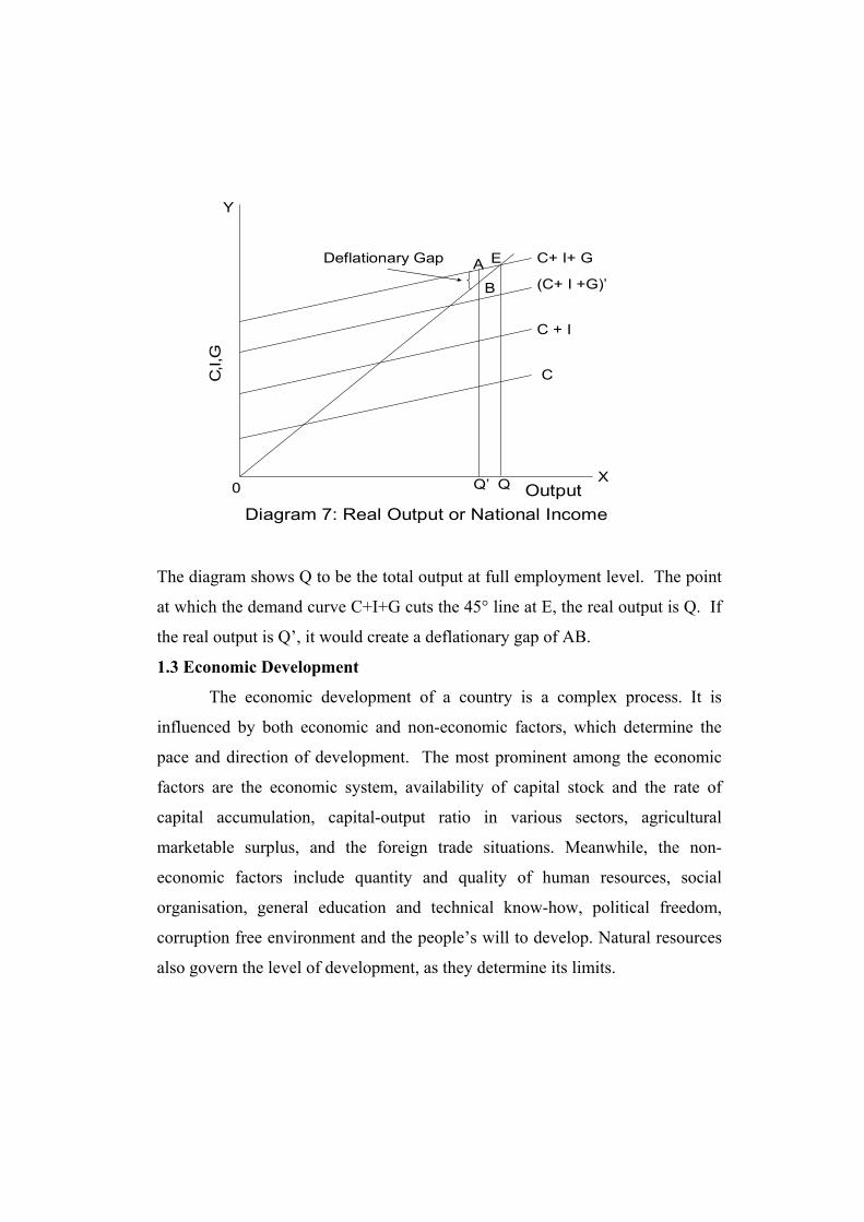
Deflationary Gap A E

B (C+ I +G)’

C + I

XQQ’

C+ I+ G

0

C,I,

GY

Output

C

Diagram 7: Real Output or National Income

The diagram shows Q to be the total output at full employment level. The point

at which the demand curve C+I+G cuts the 45° line at E, the real output is Q. If

the real output is Q’, it would create a deflationary gap of AB.

1.3 Economic Development

The economic development of a country is a complex process. It is

influenced by both economic and non-economic factors, which determine the

pace and direction of development. The most prominent among the economic

factors are the economic system, availability of capital stock and the rate of

capital accumulation, capital-output ratio in various sectors, agricultural

marketable surplus, and the foreign trade situations. Meanwhile, the non-

economic factors include quantity and quality of human resources, social

organisation, general education and technical know-how, political freedom,

corruption free environment and the people’s will to develop. Natural resources

also govern the level of development, as they determine its limits.

a) Economic factors:

Economic factors play a decisive role in a country’s economic

development. For instance, the growth of a country is generally determined by

the stock of capital and the rate of capital accumulation. The other economic

factors which influence development are the nature of economic system, the

availability of surplus food grains or food security for the people, foreign trade

situations, etc. It is important to examine the role of some of these factors in

economic development.

i) Economic system:

The historical background and economic system of a country also influences its

developmental prospects. It decides the institutional structure of a country.

Laissez faire economic system was one of its earliest forms, wherein the market

forces determined the economic progress. In today’s world, no country can

claim to be having a pure economic system, whether capitalist or socialist. With

the onset of liberalization policy, it is even more difficult to categorize countries

under clear-cut economic system. The history of economic development of any

country is inter-woven with the complex process of development, which has

helped each of them to evolve their own path of development. Thus, economic

system of a country plays a crucial role in determining the process, pace and

level of development.

ii) Capital formation:

The strategic role played by capital in increasing the level of production is

widely recognized, more so since the development of growth economics in the

post-World War II period. Capital was treated as the crucial factor of economic

growth in the Harrod-Domar growth model. At present, it is widely

acknowledged that capital accelerates the pace of growth of a country. It is

emphasized that the principal obstacle to growth is the lack of adequate capital

for investment, without which no developmental plan can be implemented

successfully. Therefore, in order to increase the level of investment, a country

has to make increased savings. This is important, as this also avoids heavy

reliance on foreign aid/capital, which can be risky.

iii) Marketable surplus of agriculture:

The excess of agricultural output produced by the sector, over and above what is

needed for the subsistence of the rural population, is known as marketable

surplus. Enhanced productivity and production in agriculture is vital for the

development of a country. These in turn should result in increased marketable

surplus of agricultural produces. Marketable surplus is particularly important in

the context of a developing country, as the rise in urban population leads to an

increase in the demand for agricultural products, mainly the food grains. These

increase in demand need to be met by adequate supplies, as scarcity of food in

urban areas would affect the process of economic growth. This is because food

shortage would force a country to import food grains, which in turn would affect

the balance of payments. India suffered a similar problem till 1976-77. Due to

inadequate marketable surplus during the period, the government of India was

compelled to import huge quantities of food grains to support the urban

population and to avert a food crisis in the country. Although this solved the

then food problem, it resulted in high foreign exchange drainage, which could

have been used for furthering the economic development of the country. To

overcome such a problem, there are countries which have embarked upon the

strategy of accelerating the pace of industrialization, so as to prevent agriculture

from lagging behind. It is for this reason that Maurice Dobb observed, “There is

reason to suppose that it will be the marketed surplus of agriculture which plays

the crucial role in the underdeveloped country in setting the limits to the

possible rate of industrialization” (Dobb 1955).

iv) Foreign trade situations:

The classical theory of trade states that international trade (particularly free

trade) benefits all the trading partners, both in terms of increased GNP and

improved welfare. Further, the theory suggests that it would benefit the less

developed countries to specialize in the production of primary products, in

which they possess a comparative production cost advantage. On the other hand,

the developed countries should specialize in the production of manufactured

goods (including machines and equipment), in which they have a comparative

cost advantage. In due course, economists like List and some of the

protectionists contradicted this idea and argued that free trade based on such

specialization would not be beneficial to a developing economy. Of late,

another school of thought has emerged under the leadership of Raul Prebisch,

who question the merits of unrestricted/free trade between developed and

underdeveloped countries on both theoretical and empirical grounds. Unlike

neo-classical economists, Prebisch argued that the relationship between trade

and development should be considered from the point of view of balance of

payments, rather than the real resource endowments. He also argued that with a

few exceptions, unrestricted trade would result in deficit balance of payments in

developing countries (Misra and Puri 2002).

b) Non-economic factors in economic development:

The non-economic factors represent the size and quality of human resources,

social organisation, general education and technical know-how, political

freedom, corruption free environment and the people’s will to develop.

i) Human resources:

Population constitutes an important factor in economic development, which is

often viewed as an obstacle to growth rather than a factor that contributes to it.

The people of a country generally make positive contributions to growth by

providing labour power for production. A country which is endowed with

efficient and skilled labour would have high productivity that would contribute

to growth. Whereas, a country with illiterate, unskilled, unhealthy and

superstitious people would generally experience low growth, as its people would

not have the capacity to contribute much to the development of its economy.

Therefore, a country that manages its manpower properly would be able to

convert its capabilities into an important factor in development. On the other

hand, if human resources remain either unutilized or underutilized due to

inefficient manpower management, the people would end up becoming a burden

to the economy rather than making positive contributions to growth. It is due to

the latter reason that in an over-populated underdeveloped country, people are

considered as a growth arresting factor.

ii) Social organisation:

People’s participation and cooperation in the development process of a country

is a pre-condition for accelerating the growth of an economy. This participation

and cooperation in development process would, however, be forthcoming only

when they are assured of the fact that the benefits of growth would be

distributed on a fair and just basis. But, experiences in numerous countries

indicate that defective social organizations have contributed to skewed

distribution of benefits of growth in society. This has resulted in some groups of

the society being benefited more than the general mass. This has resulted in

dissatisfaction among the latter class towards the development programmes of

the government, due to which the people are reluctant to participate in the

development projects initiated by the state.

India’s development experiences during the plan periods reflect such a

situation, which has led to the growth of monopolies in industries and

concentration of economic power in the hands of a few in the modern sector.

Further, the new agricultural strategy has also been more favourable to the rich

peasantry class, which has resulted in the emergence of widespread disparities in

the rural sector. This indicates that the government policies of India have also

resulted in development, which is far from being fair and just. This proves that

India’s social organisation has failed to improve along the developmental

process of the country. Therefore, although the government has been

emphasizing upon participatory development since the early plan periods, not

much success has been achieved by the country in this direction. Hence, there

has been widespread apathy towards development planning in the country,

which needs to be rectified.

iii) General education and technical know-how:

During 1909 and 1949, Robert M. Solow found the contribution of education to

be greater than that of any other factor in increasing the output per man hour in

the United States (Solow 1957). In recent times, some of the economists like

T.W. Schultz, A.K. Sen and others have stressed upon the contribution of

investment in man for economic development (Schultz 1977 and Sen 1972).

They call for development of human capabilities through human capital

investments. Although it is difficult to subject its contributions to quantitative

measurement, the results of its verifications undertaken using proxy variables

provide a tentative approximation of it.

Further, the direct impact of the level of technical know-how on the

developmental pace of a country is widely recognized today. Advancements in

the scientific and technological knowledge help man to discover more

sophisticated techniques of production that would contribute to enhanced levels

of productivity. In fact, Schumpeter attributed most of the capitalist

development to the role played by the entrepreneurial class in contributing to

technological innovations (Schumacher 1978). This recognition has led to the

consciousness towards increased investments on Research and Development for

the development of highly sophisticated technology and its further advancement.

Any country that neglects it in modern times, tends to suffer industrial

underdevelopment, low productivity and poor competitiveness in the

international market.

iv) Political freedom:

World history of modern times bears witness to the fact that the processes of

development and underdevelopment are interlinked, rather than being isolated.

It is a well known fact that the underdevelopment of past British colonies, like

Sri Lanka, India, Bangladesh, Pakistan, Kenya, Malaysia and other countries,

are all directly linked with the development of England, which indiscriminately

stripped these countries of their development and appropriated huge shares of

their economic surplus. Although these countries made a significant

contribution to Britain’s economic development, they were pushed back into

remaining backward. Another such example is that of the U.S.A.’s development

being linked with the underdevelopment of Latin American countries,

Netherlands’ development being linked with the underdevelopment of

Indonesia, France’s development being linked with the underdevelopment of

Algeria and Indo-China, and the like (Misra and Puri 2002). Hence, this

indicates that a country’s level of development cannot be clearly understood by

viewing it in isolation from that of the others with which it was historically

linked in the past.

v) Corruption:

Corruption is rampant and ailing the development process of most of the world’s

developing countries at various levels of their operations. This tends to

negatively affect their growth process and acts as a retarding factor, which slows

the pace of their development. In the process, the scarce resources allocated for

development purposes thus tend to be misappropriated, which in turn affects the

achievement of planned targets. Hence, unless corruption is rooted out of the

administrative system of these countries, it is difficult for them to grow at the

desired pace, no matter how well-formulated plan/policies they have. As a

consequence of corruption, the vested interest groups like capitalists, traders and

other powerful economic classes would continue to exploit the nation’s

resources to their personal gains. A huge chunk of the plan outlay on

development projects end up being misappropriated by the government officials

and the associated functionaries through the adoption of corrupt methods. The

regulatory system also tends to be misused quite often to obtain favours like

grant of licenses, which may not be done on the basis of merit. Tax evasion is

another major problem perfected by certain sections of the society in connivance

with some of the corrupt government officials in most of the less developed

countries, which further tends to hamper the pace of development for want of

the required revenues. However, this fact has hardly received any attention in

the literature on development and underdevelopment as a growth arresting factor

in recent years. Economist Gunnar Myrdal has been very critical about this

approach, who feels that rather unfortunately economists have deliberately

ignored the role of corruption as a retarding factor in their analysis of

development problems in the backward economies since the post-World War II

period. He identified two main reasons responsible for this: first, the presence

of diplomacy in economic research; and second, the application of Western

models which do not reflect the actual realities of the developing countries, and

have thus blurred the perspective (Myrdal 1968).

vi) Desire of the people to develop:

According to Richard T. Gill, “The point is the economic development is not a

mechanical process; it is not a simple adding up of assorted factors. Ultimately,

it is a human enterprise. And like all human enterprises, its outcome will

depend finally on the skill, quality and attitudes of the men who undertake”

(Misra and Puri 2002). This clearly indicates that development activity is not

merely a mechanical process. The pace of economic growth of any country is to

a large extent governed by the desire of its people to develop. The people of a

country who consider poverty as their fate and resign to it can never be helped,

which in turn would affect its economic growth. In the process, there would be

little hope for the development of the country.

1.4 Technological Progress and Development:

Technology refers to the knowledge about production process and machines. It

refers to the body of “skills, knowledge and procedures for making, using and

doing useful things” (Misra and Puri 2002). Thus, it includes the methods used

in the production of marketed and non-marketed commodities. “It includes the

nature and specification of what is produced, the product design, as well as how

it is produced. It encompasses managerial and marketing techniques as well as

techniques directly involved in production. Technology extends to services like

administration, education, banking and the law; besides manufacturing and

agriculture (Misra and Puri 2002). Technological progress is the change in the

technology taking place over time, in terms of process or product innovations,

which renders some earlier technologies obsolete. Process innovation results in

change in the production technique, while product innovation refers to change in

the packaging, colour, fragrance or size of the products.

Technology plays a crucial role in the economic development of a

country. Sophisticated technology has been responsible for the development of

most of the developed countries, like Japan, the United States and Western

Europe. The underdeveloped countries, which do not undertake independent

scientific research to develop their own technology suited to their own human

and natural resources, face difficulties in adopting the borrowed capital-

intensive technical know-how of the developed countries.

The technologies of production in underdeveloped countries are

backward, which determines the limits of their production capabilities, and thus

the level of development. While farmers in the developing countries, like Asia,

Latin America, and Africa, still adopt obsolete or backward cultivation

technologies, those in the developed countries, like America and Europe, adopt

mechanized cultivation technologies. In the less developed countries, machines

like tractor, harvester, etc., are being used these days, which however remain

restricted to a few selected activities, areas and section of farmers, such as the

large farmers. In recent years, nevertheless, increasingly land augmenting

technologies are being used in a number of less developed countries. Besides,

the production technologies are also fast changing in the modern large-scale

industries. For instance, in the case of industries like iron and steel, oil

refineries, heavy engineering, chemicals, and machine tools use the most

sophisticated techniques. Meanwhile, the small-scale and cottage industrial

sector, however, largely remain labour-intensive in nature or adopt intermediate

technology. Government policy, besides economic reasons are responsible for

the adoption of the labour-intensive techniques in the small-scale industrial

sector. The rationality of this policy under is to utilize the large labour force in

the country. Hence, these industries continue to use labour-intensive techniques

in the underdeveloped countries. This, however, while reflecting backwardness,

also acts as a major obstacle to the prospective economic development in these

countries.

1.4.1 Choice of techniques:

The choice of appropriate technology is a crucial issue for any underdeveloped

country. However, since all underdeveloped countries are not similar and are

experiencing different stages of development, no single technology can be

prescribed for all underdeveloped countries. This is due to the fact that a

technology which may be suitable to one country may not be equally suitable for

all the others. Therefore, the question of choice of techniques is complex and

must be analysed carefully. For this, clarity on the model of the underdeveloped

country is necessary, for which the appropriate technique is being considered.

For instance, for a country like India, which has labour as abundant factor of

production, the choice of technique should take into account the development

model of the Indian economy? Obviously, due to the huge population in the

country, labour-intensive technology is considered the most appropriate one.

This leads to the problem of making a choice between labour-intensive and

capital-intensive technology for the country. Considering the abundant labour

endowment, it is obvious that the choice should be in favour of labour intensive

technology and against the capital intensive technology, because otherwise a

large number of people would remain unemployed. The choice of technique

would then be based on the argument that this would keep the social cost low.

Hence, in countries like India, labour-intensive technology is more preferred to

the capital-intensive technology.

However, A.K. Sen is of the opinion that the problem of adopting

labour-intensive technology could be much more complex than what it appears,

because increase in labour employment would increase the wage bill, which in

turn would raise the consumption expenditure. He argued that, It is, thus,

possible that while the choice of a more labour-intensive technique will add to

output, it will add more to consumption, reducing the volume of investible

surplus. If the policy objective is the maximization of the growth rate, we may

choose more capital-intensive techniques than when it is the maximization of

immediate output per unit of investment. If our objective is something

intermediate between the maximization of immediate output and the

maximization of growth rate, we might choose techniques which are in between

these (A.K. Sen 1972).

1.4.2 Quality of labour supply:

Considering the conditions of labour supply in underdeveloped

countries, it is obvious that India and other highly populated countries should

adopt production technologies that absorb the abundant labour available in these

countries rather than capital. This implies that under the adoption of such a

production technology, a small quantity of capital per unit of labour would be

employed, which need not necessarily be true. This is because in a production

process, both fixed and variable capitals are used. If the technique involves a

greater ratio of variable capital to fixed capital, the possibility is that the

technology would be capital-intensive in nature, even though the country does

not depend much on heavy machines. However, such a situation may arise

rarely in practice. Therefore, it is quite logical to assume in the absence of

abundant capital supply, that a country would adopt labour-intensive technology

rather than a capital-intensive one.

The basic argument that a labour-intensive technology should be adopted

by highly populated underdeveloped countries is justified on two important

grounds:

a) labour supply is high, and

b) the real wage rates are very low in these countries.

Therefore, the implications of excess labour supply is that as the unemployed

labour in such countries have no opportunity cost from the social point of view,

a technology that absorbs the abundant labour in a large quantity should be

adopted. Thus, the prevailing factor abundance in India warrants that the

country goes in for the adoption of labour-intensive technology. However,

situations are different in the African and Latin American countries, which are

thinly populated. Further, in some of the underdeveloped countries where

unemployment is low, any attempt made to employ more labour by one sector

would result in their withdrawal from the other sectors. Workers under such

situations are said to possess an opportunity cost. Therefore, a labour-abundant

country should pursue a suitable policy of employing labour in such sectors,

where its productivity would be higher. This provides valid economic reasons

as to why the labour surplus underdeveloped countries should go in for the

adoption of a labour-intensive technology, even though this may not be an

appropriate strategy at higher levels of economic development. Hence, it is

sometimes argued that a rise in current output need not necessarily be the main

objective of an economic policy, because this objective may be in contradiction

with the objective of long-term economic growth. This implies that an attempt

to increase output in the short run may have an undesirable impact on the long-

term economic growth of a country. It is for this reason that some of the

developing countries take special care in choosing the technology that would

contribute to maximization of their growth rate.

1.4.3 Labour in combination with capital-intensive technology:

Labour utilization in developing countries may also create situations and

conditions that encourage the adoption of capital intensive technology. The

following need to be considered in this context:

(1) Both the price and efficiency of labour may be low in the developing

countries, due to low skill and training, malnutrition, knowledge, poor adherence

to factory discipline, or high rate of absenteeism. According to Kindleberger,

Even where nutrition is not a problem, the uneducated, undisciplined worker

will not be readily used in large-scale production with simple machinery, since

his efficiency is too low to compensate for his low wages (Kindleberger 1965)

(2) Labour also in some developing countries tends to be high-priced.

According to Kindleberger, “When the demonstration effect has extended into

the field of social services and collective bargaining, the price of labour,

including wages and benefits, will be high despite low productivity (Misra and

Puri 2002). Besides, inflation also tends to push up labour wages, while imports

of foreign capital equipments often tend to be subsidized to encourage industrial

growth in the country. Besides, government and/or labour trade unions also tend

to artificially raise up labour cost for economic or political reasons. This is the

reason why that labour need not be cheap nor capital be expensive, based on the

factor abundance or scarcity in the developing countries.

(3) Further, skilled labour and managerial expertise being in short supply in the

developing countries, it calls for an optimum combination of labour with capital

in these countries, rather than a mere maximization of labour use.

(4) Besides, Labour in some situations is less dependable and causes production

interruptions and quality maintenance problems, which encourages the use of

more capital-intensive technologies to reduce labour usage (Misra and Puri

2002).

1.4.4 Imported capital-intensive technology:

At times, a developing country ends up using capital intensive technology

despite its factor endowments favouring the adoption of labour-intensive

technology, because the technology it imported from developed country tends to

be capital-intensive. This situation arises because capital is cheap and labour

relatively scarce and expensive in the developed countries. Hence, the

technologies in the developed countries tend to have a distinct labour-saving

bias. As a consequence, the developing countries which trade from them have

to import the capital-intensive technology.

1.4.5 Labour-intensive technology:

The adoption of labour-intensive technology immediately generates increased

employment and output, when compared to the capital-intensive technology.

Hence, it is best suited for the countries with the objective of maximization of

immediate employment and output levels. Further, it is difficult to solve the

problem of unemployment in a labour abundant developing country without the

adoption of labour-intensive technologies to absorb the surplus labour supply in

it. Another important objective of the developing countries is the immediate

maximisation of output levels, which are in extremely short supply in them.

These shortages can best be taken care of by adopting labour-intensive

technology, because the gestation lag in its case is also shorter when compared

to that of the capital-intensive technologies. As a result, the former add to the

volume of output faster than the latter. Moreover, another favourable aspect of

the labour intensive technologies is that they involve no foreign exchange

requirements, whereas the capital-intensive technologies require imports of

substantial capital equipments from foreign countries and substantial

maintenance of the imports later as well. Hence, the developing countries which

lack foreign exchange resources should therefore choose labour- intensive

technologies.

1.4.6 Appropriate technology:

In recent years, the issue of appropriate technology for the developing countries

has caught the attention of the policy makers, economists and planners. This is

attributable to the fact that huge import of capital-intensive technology by the

developing countries from the developed countries over the past few decades

have also failed to yield the desired growth and development in them. Such

import of technology by them have largely resulted in the development of

certain towns and major cities, created a few employment opportunities, and left

the smaller towns and rural areas lagging behind, such that large number of their

residents continue to remain poor, unemployed and underemployed. Besides,

the cost of every additional employment created through the adoption of the

imported technology also becomes very high, which is more suited to the

advanced countries with their high per capita income, a low population growth

rate, and high saving to income ratio. However, for the developing countries

which have acute shortage of investment resources for creating infrastructure

and building industries, insufficient foreign exchange resources, and high

construction and equipment cost, such a technology tends to be inappropriate.

Given the high rate of population growth, a growth strategy based on industry-

led development using the technologies suited to developed countries only

creates poverty, unemployment and underemployment in the developing

countries. Thus, it is the responsibility of the developing countries to work out

and adopt an appropriate technology, most suited to the available natural

resources, human capital, socio-economic features, etc., which would contribute

to its growth and development.

1.4.7 Intermediate technology:

Owing to the failure of intermediate technology to generate the desired effects in

overcoming the problems of poverty and unemployment in the developing

countries, some economists have recommended the use of intermediate

technology by them. For, the gap between the technologies of developed and an

underdeveloped country is so wide, that the latter can achieve little success by

adopting the advanced technologies of the former. This is attributable to two

major reasons:

(i) Technology of the developed countries is too expensive for the

underdeveloped countries, which lack the required resources; and

(ii) The adoption of such advanced technologies would only aggravate the

already existing problems of poverty and unemployment in these countries.

According to E.F. Schumacher, it is a serious error to assume that

whatever technology is appropriate to developed countries of the West is equally

appropriate to developing countries of the Third World. Granted that the

technological backwardness is the main cause of poverty of underdeveloped

countries and their traditional techniques of production would not survive long,

nonetheless, it cannot be concluded that the most sophisticated technology of the

developed West is appropriate to the poor countries. This fact must not be

overlooked that in all those countries where mechanization has been done on a

grand scale, capital has been available in abundant supply, while labor has

been a relatively scarce factor (Schumacher 1978). This explains the increasing

adoption of automatic machines by the developed countries. On the other hand,

there is surplus labour supply in the underdeveloped countries, while the capital

stock is limited. Owing to these practical problems, it is difficult for the labour

surplus developing countries to adopt the highly sophisticated capital-intensive

technologies of the developed countries.

Meanwhile, it is undoubtedly true that the adoption of sophisticated

technology would certainly prove advantageous in some of the sectors of the

developing countries. However, Schumacher feels that such sectors would not

account for more than 15 per cent of the whole economy, while the remaining

85 per cent of the economy would have to depend upon, what he called as the

‘intermediate technology’. Schumacher emphasized that intermediate

technology was superior to the traditional technologies of the less developed

countries, which were simple and less expensive compared to those of the

developed countries.

However, the possibility of the development of intermediate technology

has frequently raised a debate on the choice of appropriate technologies, as most

often the capital-intensive technology of the developed countries is viewed as an

alternative to the traditional labour-intensive technology of the developing

countries. Despite this fact, few developing countries, including India, have

made serious attempts to identify and develop intermediate technology, which

have also proved to be quite successful when connected to the sophisticated

technologies of the developed countries. Thus, the opinion that the capital-

intensive technology suited to the developed countries would also be suitable to

all other countries is wrong. In fact, it is the specific conditions of a particular

country which determine the appropriateness of a technology for it.

1.5 Business and Government

There are several ways in which the government may influence business

operations in a country. Some of them may be discussed here.

(a) Government enterprises:

Sometimes, government may directly involve in the production of private or

marketable commodities or services, because the private sector does not supply

them in optimum amounts. Optimum level of output is the maximum output

produced at the full productive capacity of a firm at minimum cost, which is

welfare maximizing. Besides, the government may also decide to set up its own

public enterprises, and produce and sell output of natural monopoly industries.

(b) Price fixation:

The state or central government can fix the price of products; either produced by

private or public sector enterprises, or may enforce price regulation for the

welfare and protection of the consumers, or revenue generation. The prices

announced by the government for the goods produced in the public sector and/or

private sector units are known as administered prices. Depending upon the

political and economic conditions, the government may raise these prices.

Examples of such administered prices are power tariff, air fare, rail fare, postal

rates, prices of petroleum products like LPG, diesel, and petrol and prices of

rice, wheat, sugar and urea, sold through the Fair Price Shops.

The government may also regulate monopoly price. Monopolies are

those producing units, who have no close substitutes. Taking advantage of their

position, they generally tend to charge a price higher than the one charged by the

competitive firms. Therefore, the government may regulate the price of the

monopoly seller and force them to become price taker. However, the monopoly

seller is free to sell the quantity that would maximize his/her profit.

The government may also announce support prices for primary

agricultural products in the interest of farmers, particularly during the periods of

surplus production resulting from technological advancement. The purpose of

support prices is to ensure that farmers do not incur any loss, when cost of

production falls. Such prices, however, interfere with the automatic

determination of market prices through the interaction of market demand and

supply. India has placed 22 farm products under minimum support price or

statutory price categories. Besides, cereal crops like rice and wheat are

procured at previously announced prices in every crop season.

(c) Direct intervention:

Tax is one of the ways in which government makes direct intervention, which

directly increases the price of a product by adding to the cost of production.

Government may impose tax to reduce production, or reduce tax or provide tax

subsidy to encourage it. Tax relief may also be given to encourage production in

strategic industries. On the other hand, higher taxes may be imposed to

discourage production of commodities which are injurious to health. In the

process, the government may also influence the consumption level of such

commodities.

(d) Indirect intervention:

The device of allocating quotas is another important method of government

intervention in the context of business enterprises. This method is generally

adopted by the developed countries, who find it more convenient to restrict

production so as to restrain the rising burden of price support to producers.

Under this method, the producers are restricted from producing output beyond a

prescribed limit by the government. If the government directive is not followed,

they would be debarred from any government policy, benefits, including that of

the price support. Thus, production quotas tend to have an upward pressure on

the price, due to restriction imposed on output supply. In sum, the expected

change from price support should be acceptable to both the producers and

consumers, such that they may be neutral towards price support and production

quota policies. Besides, the government also controls inflation through the price

regulation mechanisms.

(e) Control of monopolies:

Monopoly enterprises are harmful to the welfare of consumers. As only one

producer controls the production under it, there is a tendency on its part to

exploit consumers by charging high prices because the product has no close

substitute. Besides, the price may also be artificially raised through under-

production. Further, monopolies also result in the concentration of economic

power in the hands of a few, which interferes with the objective of just and

equitable distribution of income and wealth. To avoid such consequences, most

governments have passed legislative acts to control their activities. The Indian

government passed the Monopoly and Restrictive Trade Practice Act in 1976 to

control them.

Thus, the government may participate in the production activities along

with the private sector in an economy, besides controlling, regulating and

governing the activities of the latter in the general interest of maximizing the

welfare of the people of the country.

References:

C.S. Barla, Managerial Economics, National Publishing House, Raipur, 2000.

Charles Kindleberger, Economic Development, McGraw Hill Book Company,

New York, 1965.

H. Craig Petersen and W. Cris Lewis, Managerial Economics, Prentice-Hall of

India, New Delhi, 2003.

K.K. Dewett, Modern Economic Theory, S. Chand and Company Ltd., New

Delhi, 2005.

Gunnar Myrdal, Asian Drama, Pantheon, 1968.

A. Koutsoyiannis, Modern Micro Economics, Macmillan Publishers Ltd.,

London, 1979.

S.K. Misra and V.K. Puri, Economics of Development and Planning, Himalaya

Publishing House, New Delhi, 2002.

Morris Dobb, “A Note on the so-called Degree of Capital-Intensity of

Investment in Underdeveloped Countries”, in On Economic Theory and

Socialism, London, 1955.

V.L. Mote, Samuel Paul and G.S. Gupta, Managerial Economics: Concepts

and Cases, Tata McGraw Hill Publishing Company Ltd., New Delhi, 2001.

Robert Solow, “Technical Change and the Aggregate Production Function”,

Review of Economics and Statistics, 1957

A.K. Sen, Choice of Techniques, Oxford University Press, 1972.

E.F. Schumacher, Small is Beautiful, Radha Krishna Prakashan, New Delhi

1978.

Theodore W Schultz, Investment in Human Capital: The Role of Education

and of Research, Free Press, New York, 1977.

Questions:

1. Define national income.

2. Illustrate the circular flow of income and expenditure using a two sector

model.

3. Explain the different concepts of national income.

4. Distinguish between national income at factor price and market price.

5. What is disposable income?

6. Define the principle of effective demand.

7. Illustrate the determination of equilibrium level of national income.

8. Does equilibrium necessarily occur at full employment level?

9. Explain the Keynesian theory of employment.

10. Illustrate the determination of equilibrium national income through the

equality of saving and investment.

11. Define marginal propensity to consume.

12. What are the determinants of investment?

13. Explain the concept of liquidity preference.

14. What is inflation?

15. Describe the concepts of inflationary and deflationary gaps.

16. Define economic development.

17. Discuss the economic and non-economic factors determining economic

development.

18. Define technology.

19. What is technological progress?

20. Examine the problem of choice of technique.

21. Distinguish between labour intensive and capital intensive technologies.

22. What do you understand by appropriate technology?

23. What is sustainable technology?

24. Write a note on government intervention and business.

Unit-V

Lesson - 1

INTER SECTORAL LINKAGES

Introduction

The three sectors of the economy are related to one another in many ways.

Agriculture depends upon industry for the supply of its inputs and implements

and Industry depends on the agriculture for the demand of its products. Services

are dependent upon both. Hence one cannot be separated from the other in the

economy.

Objectives

By studying this lesson the students will be in a position to understand the inter

linkage of one sector of the economy to the other. How agriculture is the back

bone of the industries and in return industries are facilitators of the agriculture.

Apart from all that what is the link between agriculture and industry on one hand

and Services on the other .The whole discussion in this lesson will highlight not

only the link between these sectors but also the interdependence of these sectors.

Contents

1. Agriculture as the provider of livelihood and employment in

underdeveloped economy.

2. Agriculture as the supplier of raw materials to the industry.

3. Agriculture as the placer of demand for industrial goods.

4. Industries as the absorber of the labour force shifted from

agriculture.

5. Industries as the provider of industrial and consumer goods to

the agriculture.

6. Industries as the provider of agricultural implements to agriculture.

7. Services as the consequence of the development of these two

Sectors and facilitator to them.

The Discussion

The debates have centered on the relative importance to be assigned to

agriculture versus industry. This dichotomy has very been overdrawn. Time has

shown the limitations of over emphasizing industrialization and at the same time

it is widely recognized that agricultural progress must have a vital role in the

development process. The past controversy and tussle between agriculture and

industry has been proved to be a false issue and the concern now is rather with

the interrelationships between industry and agriculture and the contribution that

each can make to the other.

In developing countries more people get engaged in agriculture for

their livelihood than in the industrial and tertiary sectors of the economy.

Agricultural growth provide food for the growing non agricultural labour force

and raw material for agro based industries, stimulates domestic demand for

industrial goods, increases savings and tax revenue to be utilized for further

development. Export of agricultural goods earns foreign exchange which is

utilized for financing imports of capital goods, intermediate goods and raw

materials for industrialization. Growth of agriculture not only helps the

development of industrialization process but also facilitates the development of

labour intensive village, medium and small scale industries in rural and urban

areas.

Development of agriculture is directly related to the increase in the

income of the rural people as about 70% of them depend upon agriculture.

Raising rural incomes have strong multiplier effects in that they increase the

demand for domestic non-agricultural goods and services which, in turn,

increase the incomes of those providing the goods and services. As rural

incomes rise due to increasing agricultural production and productivity, the

increase in the domestic demand for agricultural goods brings rapid gains for

industrialization . Apart from that, growth in the industrial output of consumer

goods needed by the rural population, the out put of fertilizers, pesticides,

agricultural tools, implements and other intermediate manufactured goods

required by the farm sector also grow. Moreover, with the diversification of

agricultural activities, a number of labour intensive village and small enterprises

are set up in the rural areas. These provide further fillip to industrialization.

While agriculture is progressing, it will provide some of the resources for

industrialization. In fact, increased agricultural productivity implies a large

marketable surplus and a redistribution of income in favor of the rural sector.

Industrialization requires the reallocation of funds towards the modern sector

along with rising agricultural incomes. Rising farm incomes are mopped up

through land taxes and betterment levis and the mobilization of rural savings

through savings drives and such financial institutions as cooperative banks, rural

banks etc. They play an important part in canalizing rural savings for

industrialization.

Development in the productivity and yield in the agriculture and thereby total

production leads to export of agricultural products which help finance large

imports of raw materials, intermediate and capital goods for industrial

production, the LDCs save the foreign exchange for industrial development.

On the other hand, industrialization helps develop agriculture in number of

ways which for the sake of better study are discussed below:-

1. Rise in demand for agricultural commodities

Industrialization leads to the rapid rise in the income of the people, which affects

rise in the demand for such agricultural commodities as milk, .vegetables, eggs,

poultry etc. Since production of such commodities is labour intensive,

agricultural production is greatly increased without enlarging farm acreage. This

in turn, provides more work to rural population and raises incomes.

2. Availability of capital

With industrialization, financial institutions develop and they finance agriculture

too and thereby availability of capital increases for the agricultural sector which

helps in modernizing agriculture and raising farm output.

3.Vast Job Opportunities

The natural consequence of industrialization is urbanization which opens

enormous job opportunities to the rural labour force that were disguisedly

unemployed in agriculture. They remit money back to the home which is

utilized for arranging inputs for agriculture and cattle raising, poultry and

fisheries etc. With the economic development and thereby urbanization,

transport sector develops and consequently market expands. Agriculturists are

facilitated by this expanded market by selling their surplus agricultural products

at remunerative prices. Many people engage in some part time job that either

live near to the town or visit the town very frequently because of nearness of the

town from the villages.

4. Change in the Attitude

When, after industrialization urbanization takes place, the air is charged in the

neighboring areas. Villagers now, have the access to the modern education,

entertainment and jobs which in turn bring a great change in their life style and

attitude.

5. Motivation to raise income

With the changed attitude, people in the villages require modern means of

comforts and luxuries as T.V, washing machines, computer, motorcycles etc.

which can be had only by raising their income. Hence, they work hard and try

their best to modernize agriculture to improve their income.

Summary

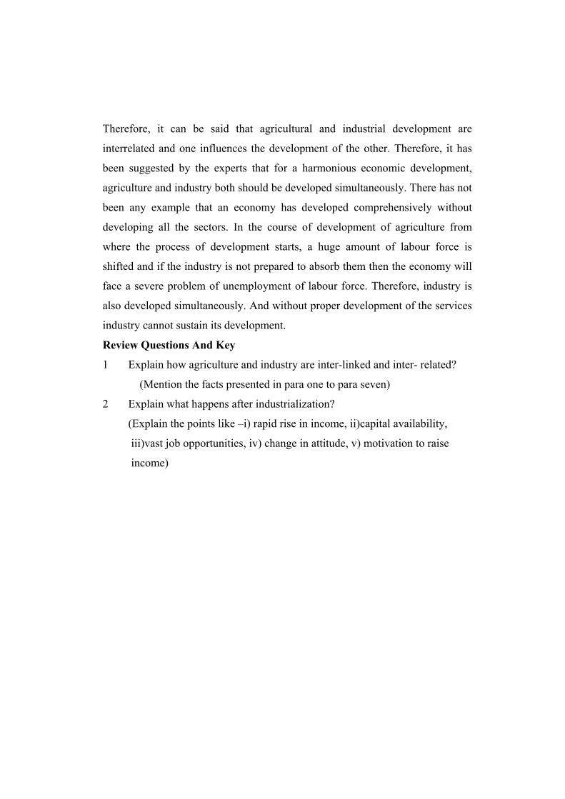
Therefore, it can be said that agricultural and industrial development are

interrelated and one influences the development of the other. Therefore, it has

been suggested by the experts that for a harmonious economic development,

agriculture and industry both should be developed simultaneously. There has not

been any example that an economy has developed comprehensively without

developing all the sectors. In the course of development of agriculture from

where the process of development starts, a huge amount of labour force is

shifted and if the industry is not prepared to absorb them then the economy will

face a severe problem of unemployment of labour force. Therefore, industry is

also developed simultaneously. And without proper development of the services

industry cannot sustain its development.

Review Questions And Key

1 Explain how agriculture and industry are inter-linked and inter- related?

(Mention the facts presented in para one to para seven)

2 Explain what happens after industrialization?

(Explain the points like –i) rapid rise in income, ii)capital availability,

iii)vast job opportunities, iv) change in attitude, v) motivation to raise

income)

Lesson – 2

NATIONAL INCOME

Introduction

Macro aggregates mean the parameters which exhibit the health of the economy.

Macro economic indicators like national income, total output, employment and

general price level etc. present the overall picture of the economy as it is in and

indicate the future direction. Hence the analysis of macro aggregates becomes

necessary to understand and assess the strengths and weaknesses of the economy

and thereby formulate the appropriate policies.

Objectives

By reading this lesson the students will be in a position to understand the macro-

economic scenario of the economy in general and individual macro-economic

sectors in particular. The performances of these sectors like national income ,

employment, general prices are the real reflector of the health of the economy

.An economy is growing of not and if growing then the fruits of development is

reaching to the people or not can be studied well by studying this lesson.

Contents

1. National income

2. Total output

3. Employment

4. General price level

1.National income

Credit goes to Prof.V.K.R.V.Rao, who was the first economist to compute the

national income of India in a scientific manner. He divided the economy into

three sectors- primary, secondary and tertiary or services.

The first scientific estimate of national income was made during 1949

with the appointment of the National Income Committee in August 1949 having

Prof. Mahalnobis, D.R.Gadgil and Prof. V.K.R.V.Rao as members. This

committee submitted its final report in February 1954in which it gave estimates

of national income for the year 1948-49. They analyzed the total national

income by industrial origin, the character of the enterprise and the net output per

employed persons in various occupations. There after, the national income

estimates of India have been prepared and published regularly by Central

Statistical Organization (CSO). The CSO follows the product and the income

methods while preparing the estimates of national income. They use product

methods for the sectors which produce commodities such as agriculture,

forestry, fishing, mining etc. and manufacturing. The income method is applied

for computing income from tertiary or services sector such as banking,

insurance, transport, trade, public services etc.

The Central Statistical Organization has revised the base year from

1980-81 to 1993-94and brought out a new series of National Accounts Statistics.

The coverage of G.D.P has been extended by including several horticultural and

floricultural crops in agriculture. In other services, estimation of income from

unorganized service activities on the basis of new NSS Employment Survey

Results, Private activities under T.V and radio, tailoring and the activities of

high value software consultancy have been included. The main purpose of

extending coverage was to reduce under reporting of G.D.P

Sectoral Share of GDP.

Table I Sectoral share of GDP

Sector 1993-94 1997-98

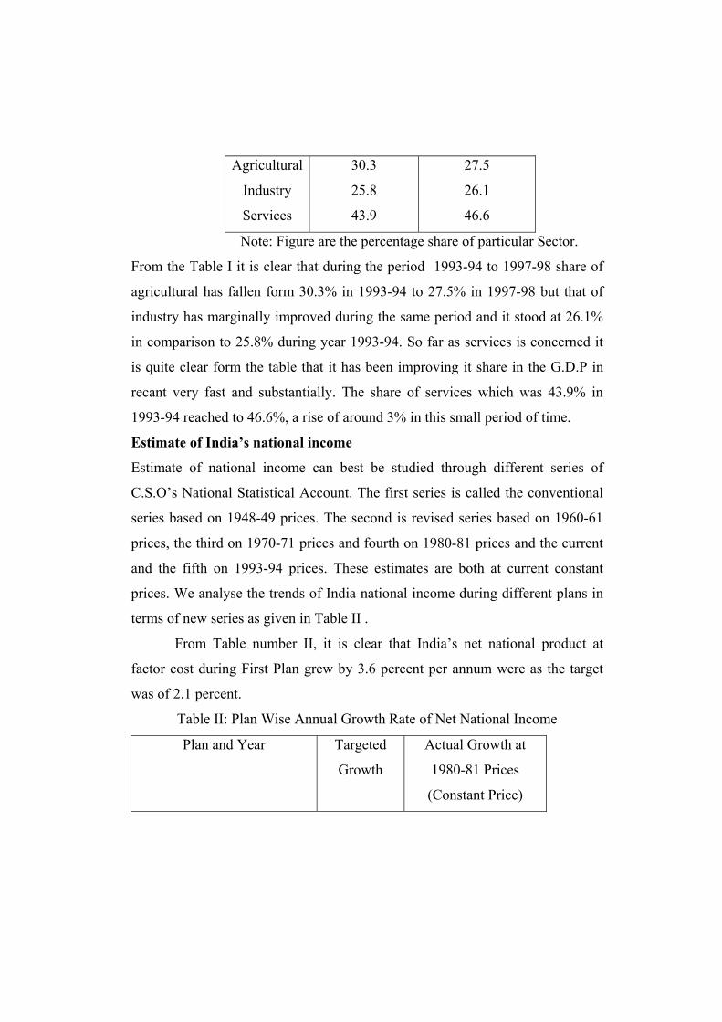
Agricultural

Industry

Services

30.3

25.8

43.9

27.5

26.1

46.6

Note: Figure are the percentage share of particular Sector.

From the Table I it is clear that during the period 1993-94 to 1997-98 share of

agricultural has fallen form 30.3% in 1993-94 to 27.5% in 1997-98 but that of

industry has marginally improved during the same period and it stood at 26.1%

in comparison to 25.8% during year 1993-94. So far as services is concerned it

is quite clear form the table that it has been improving it share in the G.D.P in

recant very fast and substantially. The share of services which was 43.9% in

1993-94 reached to 46.6%, a rise of around 3% in this small period of time.

Estimate of India’s national income

Estimate of national income can best be studied through different series of

C.S.O’s National Statistical Account. The first series is called the conventional

series based on 1948-49 prices. The second is revised series based on 1960-61

prices, the third on 1970-71 prices and fourth on 1980-81 prices and the current

and the fifth on 1993-94 prices. These estimates are both at current constant

prices. We analyse the trends of India national income during different plans in

terms of new series as given in Table II .

From Table number II, it is clear that India’s net national product at

factor cost during First Plan grew by 3.6 percent per annum were as the target

was of 2.1 percent.

Table II: Plan Wise Annual Growth Rate of Net National Income

Plan and Year Targeted

Growth

Actual Growth at

1980-81 Prices

(Constant Price)

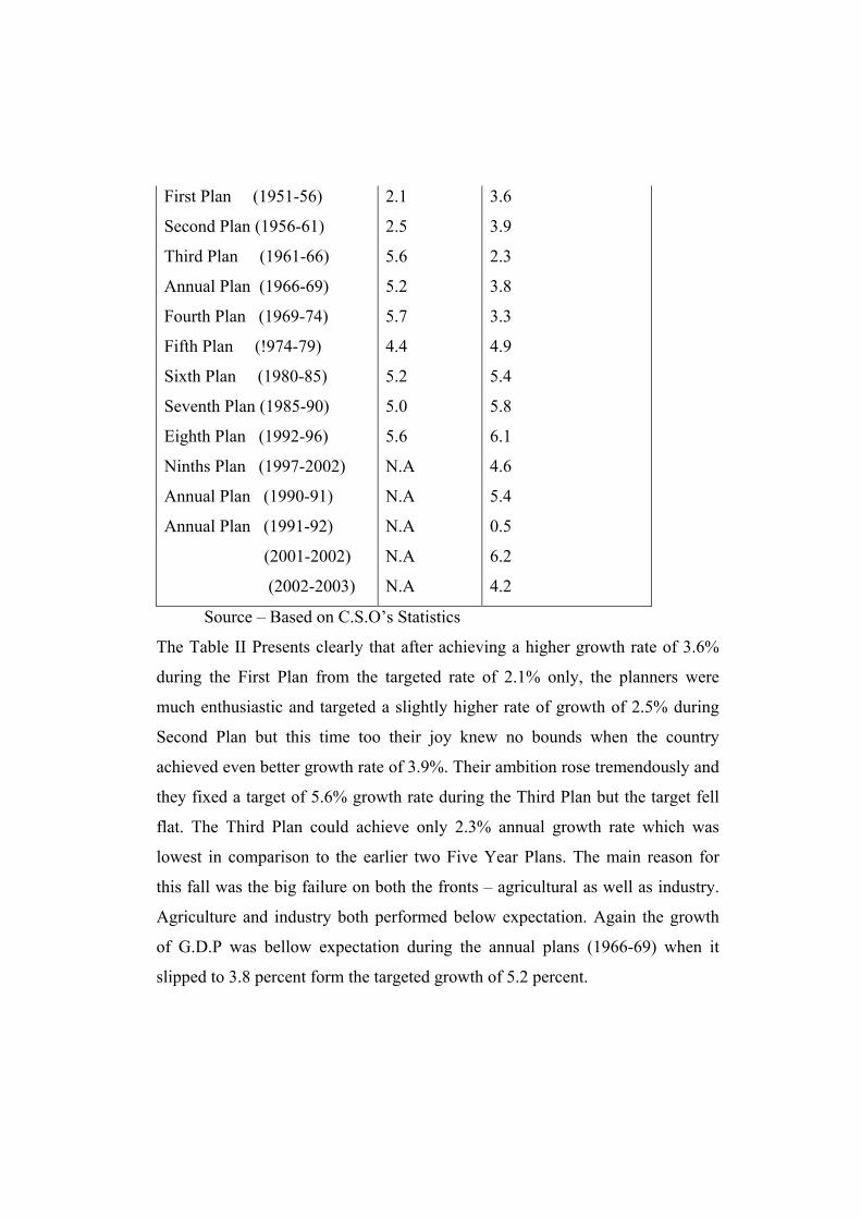
First Plan (1951-56)

Second Plan (1956-61)

Third Plan (1961-66)

Annual Plan (1966-69)

Fourth Plan (1969-74)

Fifth Plan (!974-79)

Sixth Plan (1980-85)

Seventh Plan (1985-90)

Eighth Plan (1992-96)

Ninths Plan (1997-2002)

Annual Plan (1990-91)

Annual Plan (1991-92)

(2001-2002)

(2002-2003)

2.1

2.5

5.6

5.2

5.7

4.4

5.2

5.0

5.6

N.A

N.A

N.A

N.A

N.A

3.6

3.9

2.3

3.8

3.3

4.9

5.4

5.8

6.1

4.6

5.4

0.5

6.2

4.2

Source – Based on C.S.O’s Statistics

The Table II Presents clearly that after achieving a higher growth rate of 3.6%

during the First Plan from the targeted rate of 2.1% only, the planners were

much enthusiastic and targeted a slightly higher rate of growth of 2.5% during

Second Plan but this time too their joy knew no bounds when the country

achieved even better growth rate of 3.9%. Their ambition rose tremendously and

they fixed a target of 5.6% growth rate during the Third Plan but the target fell

flat. The Third Plan could achieve only 2.3% annual growth rate which was

lowest in comparison to the earlier two Five Year Plans. The main reason for

this fall was the big failure on both the fronts – agricultural as well as industry.

Agriculture and industry both performed below expectation. Again the growth

of G.D.P was bellow expectation during the annual plans (1966-69) when it

slipped to 3.8 percent form the targeted growth of 5.2 percent.

Irrespective of a failure during annual plans, Indian planner fixed an

ambitious target of 5.7% G.D.P growth during Fourth Plan but what could be

achieved was only 3.3%, even lesser than annual plans. Therefore a close

analysis of the table reveals that except for Sixth, Seventh and the Eighth Plans,

targeted growth was never realized.

Summary

Prof. V.K.R.V.Rao was the first economist to compute India’s national income

in a scientific manner. National income committee was appointed in 1949 and it

gave estimate in 1954. The base year has been shifting. The CSO which is

responsible for publishing national income estimates follow the income and

product methods while preparing the national income estimates.

The share of different sectors in national income has been changing over

the years. The share of agriculture was 30.3 percent in 1993-94 fell down to 27.5

percent in 1997-98. During the same period the share of services in national

income increased from 43.9 percent to a high of 46.6 percent.

Except for the few years India’s national income has been growing

steadily at around 4 percent. It was highest at 6.2 percent during the years 2001-

2002 and lowest at 0.5 percent during the years 1991-92.

Review Questions and Key.

1 Point out the procedures adopted in the estimation of India’s national

income.

(Refer to I and II para of this lesson)

2 Explain the plan wise growth of India’s national income.

(Refer to the table No. II)

LESSON – 3

EMPLOYMENT

EMPLOYMENT IN ORGAINSED AND UNORGANISED SECTOR

Introduction

Employment is another indicator of the health of the economy. Employment is

directly related with the national income because a higher employment will be

followed by a higher output and thereby income. Not only that, a higher level of

employment encourages advancement in education, skill formation, human

resource development and a better physical quality of life. Hence, study of

employment helps us to estimate the real status of the economy.

Objective

Reading this lesson, students will be in a position to understand employment

potential of various sector of the economy, rise and fall of employment in

different sector income generation, performance of different Plans on

employment front etc.

Contents

* Growth rate of employment in different sectors

* Employment in organized and unorganized sector

Growth Rate Of Employment In Different Sectors

The growth rate of employment which was 2.04% per annum during the ten

year’s period of 1983 to 1993-94, declined sharply to 0.98 percent during 1993-

94 to 1999-2000. Therefore, it is told that the economic growth in this period

was of jobless variety. Sector wise growth of employment has been explained in

the table III.

Table III – Sectoral Growth of Employment 1983-2000

It is clear from the above table (No-III) that the growth of employment in the

primary sector during 1983-94 was only 1.6 percent and that during 1994-2000

become negative i.e. -0.34% The contribution of the primary sector in terms of

providing employment was very important as ever which stood at 208.99,

245.16 and 239.83 millions during the period 1983, 1993-94 and 1999-2000

respectively. So far as secondary sector is concerned it’ contribution towards

employment has been consistent at 13.8,14.8 and 16.8 percentages respectively

during the reporting period. The growth of employment in this sector during

Sector Employed Workers (million) Annual Growth

Rate(%)

1983 1993-94 1999-

2000

1983-84 1994-

2000

Primary

Secondary

Tertiary

208.99

(69)

41.66

(13.8)

52.11

(17.2)

245.16

(65.5)

55.53

(14.8)

73.76

(19.7)

239.83

(60.4)

66.91

(16.8)

90.26

(22.7)

1.16

2.90

3.53

-0.34

3.14

2.42

Total

Employment

302.76

(100.0)

374.45

(100.0)

397.00

(100.0)

2.04

0.98

1983-94 and 1994-2000 were 2.9 and 3.14 percent which can be said as

satisfactory. But remarkable was the growth of employment in the tertiary sector

where it grew from 52.11 million jobs in 1983 to 73.76 million during 1993-94

and hopping 90.26 million during 1999-2000 having the percentage of 17.2,

19.7 and 22.7 respectively.

By organized sector it is normally understood as public sector but the private

sector is also included where at least 10 or more workers work at a time.

Table IV- Total organized Sector Employment

It is evident form the table IV that over the years since 1983-2000 the volume of

employment has increased form 302.75 million to 397.00 million. Though the

growth during 1983-94 was at 1.6%, which became negative during 1994-2000;

the early liberalization era. The contribution of public sector remained almost

around 70% and that of private sector around 30%.

Employment In Organised And Unorganized Sectors

Growth Rate %

Per Annum

1983 1988 1994 1999-00 1983-94 1994-00

a) Total

Employment

302.75 324.29 374.45 397.00 2.04 0.98

b) Public

Sector

16.46

(68.6)

18.32

(71.3)

19.44

(71.0)

19.41

(69.1)

1.52

-0.03

c) Private

Sector

7.55

(31.4)

7.39

(28.7)

7.93

(29.0)

8.70

(30.9)

0.45 1.87

(B+C) 24.01 25.71 27.37 28.11 1.20 0.53

Summary

From the above discussion it becomes clear that the growth rate of employment

in recent years has fallen. While it was 2.04% during the ten years period of

1983-84 to 1993-94, declined sharply to 0.98% during 93-94 to 1999-2000. The

major contributor in employment front has been the primary sector which has

been consistent in providing employment to around 65%. Within organized

sector the Public sector has been the major provider of employment at around

19%.

Review Questions and Key

1. Explain the growth rate of employment in different sectors.

(Refer Table No. III)

Show the contribution of organized and unorganized sectors towards

employment. (Refer table no. iv)

Lesson – 4

GENERAL PRICE LEVEL

Introduction

The study of general price level is another indicator of the health of the

economy. Price level and purchasing power have inverse relationship.

Increasing prices reduce people’s purchasing power and thereby bring hardship

and fall in general welfare. Hence, every government tries to keep the rate of

inflation under acceptable level so that economic activities are also induced and

people’s parching power too remains high. Therefore, rise in real income of the

people can be analyzed through the rise in inflation.

Objective

Reading the trend of general price level will enable us to analytically reach to a

conclusion as to what had been the level of real economic development in the

country.

Contents

Price situation during 1979-80 to 1989-90. Price situation after liberalization.

Causes of price rise.

Table V. Price situation during 1979-80 to 1984-85

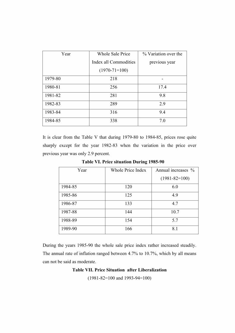
It is clear from the Table V that during 1979-80 to 1984-85, prices rose quite

sharply except for the year 1982-83 when the variation in the price over

previous year was only 2.9 percent.

Table VI. Price situation During 1985-90

Year Whole Sale Price

Index all Commodities

(1970-71=100)

% Variation over the

previous year

1979-80 218 -

1980-81 256 17.4

1981-82 281 9.8

1982-83 289 2.9

1983-84 316 9.4

1984-85 338 7.0

Year Whole Price Index Annual increases %

(1981-82=100)

1984-85 120 6.0

1985-86 125 4.9

1986-87 133 4.7

1987-88 144 10.7

1988-89 154 5.7

1989-90 166 8.1

During the years 1985-90 the whole sale price index rather increased steadily.

The annual rate of inflation ranged between 4.7% to 10.7%, which by all means

can not be said as moderate.

Table VII. Price Situation after Liberalization

(1981-82=100 and 1993-94=100)

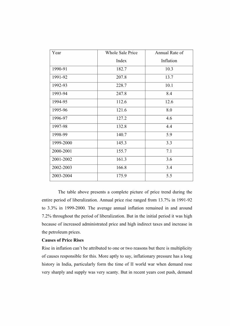
Year Whole Sale Price

Index

Annual Rate of

Inflation

1990-91 182.7 10.3

1991-92 207.8 13.7

1992-93 228.7 10.1

1993-94 247.8 8.4

1994-95 112.6 12.6

1995-96 121.6 8.0

1996-97 127.2 4.6

1997-98 132.8 4.4

1998-99 140.7 5.9

1999-2000 145.3 3.3

2000-2001 155.7 7.1

2001-2002 161.3 3.6

2002-2003 166.8 3.4

2003-2004 175.9 5.5

The table above presents a complete picture of price trend during the

entire period of liberalization. Annual price rise ranged from 13.7% in 1991-92

to 3.3% in 1999-2000. The average annual inflation remained in and around

7.2% throughout the period of liberalization. But in the initial period it was high

because of increased administrated price and high indirect taxes and increase in

the petroleum prices.

Causes of Price Rises

Rise in inflation can’t be attributed to one or two reasons but there is multiplicity

of causes responsible for this. More aptly to say, inflationary pressure has a long

history in India, particularly form the time of II world war when demand rose

very sharply and supply was very scanty. But in recent years cost push, demand

pull and structural factors have been mainly responsible for this. Expanding

demand for goods and services is due to the ever rising population of the

country, rising money incomes, expansion in money and liquidity in the

economy, rising volume of black money etc. on the other hand, supply side of

the economy is also equally responsible for this. Supply of goods and services

has not risen in the proportion as the demand. This may be due to failure of

monsoon, bottlenecks in transport, power, shortage of various inputs etc.

Summary

The study of price level indicates about the purchasing power of the people. It

also indicates about the real upliftment in the general standard of living of the

people. When we look to the rise in prices form 1979-80 to 1984-85 we find that

during the years 1980-81, general price level increased by the highest 17.4

percent. In the period between 1985-90 based on 1981-82 prices the general

price level increased by highest 10.7 percent during 1987-88. After liberalization

the general price level rose highest by 12.6 percent during the years 1994-95.

There were different causes for the rise in prices. The prominent among them

were imposition of additional taxes, financing of development projects, public

debt, deficit financing, social security burden, infrastructural development etc.

Review Question and Key

1. Explain the price situation in India during 1979-80 to 1985-90.

(Refer Table No.V and VI)

2. Explain the price situation after liberalization

( Refer Table No.VI)

3. Point out the various causes for the rise in general price level

(Mention the point I to X in the sub heading – causes for price rises).

Lesson - 5

FISCAL POLICY AND FULL EMPLOYEMNT

Introduction

Fiscal policy is a part of general economic policy of the government, which is

primarily concerned with budget receipts and the expenditure of the

government. Fiscal policy explains the tax and expenditure policy of the

government. It encompasses two separate but related decisions, public

expenditures and the level and structure of taxes. The amount of public outlay,

the incidence and effects of taxation and the relation between expenditure and

revenue exert a significant impact upon free enterprise economy.

Objectives

Attaining full employment

Leveling the gap of income distribution

Economic stabilization

Economic Growth

Contents

Fiscal policy and economic growth

Fiscal policy and full employment

Fiscal policy and Social justices

Fiscal policy and Economic stabilization

Role of fiscal policy in developing countries.

Fiscal Policy and Economic Growth

Developed economies aim at attaining full employment through long term fiscal

policy. .Keynesian analysis of fiscal policy is considered as short term view

where as post Keynesian economists like Hanson, Harrod and Domer have tried

to extend Keynesian analysis to a more comprehensive long term theory of

income and employment. Therefore, the main objective of long term fiscal

policy in developed country is conceived to be the maintenance of a steady

growth of full employment income with out inflation or deflation in order to

avoid secular stagnation or secular inflation.

According to Harrod and Domer, investment plays a vital role in the

process of economic growth. In the process of secular growth, along run

disequilibrium may occur in a mature economy. The reason behind this

disequilibrium may be the income does not grow at a rate just sufficient to

ensure full capacity use of a growing capital stock. Thus, the objective of growth

and full employment in the long run is associated with problem of enlarging

capacity through investments in capital goods sector. Therefore, in the long run,

employment is the function of the rate of growth, investment and income.

But the role of fiscal policy in a developing country is different because

this type of countries are caught in the grip of vicious circle of poverty, and

quite obviously the aim and objective of long term fiscal policy in these

countries should be breaking the vicious circle of poverty. Rapid economic

growth is the long term objective of fiscal policy in poor countries and thereby

to break the circle.

Fiscal policy aims at fulfilling following objectives while used as a

means of encouraging economic growth:

Providing revenue to public enterprises.

Imposition of additional taxes

Realizing and channelizing the potential resources into productive projects.

Direct physical control.

Increase in the rate of taxation.

Public dept.

Deficit financing.

To promote investment into socially desirable channels.

Inducing and stimulating private investment.

To change the direction and pattern of investment and production so that

general economic welfare is improved and to level the gap of the distribution of

wealth and income. (reframe the highlighted sentence)

Fiscal Policy and Full Employment

According to Keynes, public finance is a compensatory finance which should

aim at full employment and to maintain it. To attain this let us see some of the

suggestions made by Keynes-

a) Deficit budget: Budgetary policy should be designed to fight deflation and

unemployment. A deficit budget will bring about expansionary effects in a

stagnant economy.

b) Tax Policy for Stimulation: The tax policy should be designed in such way

that it stimulates consumption and investment both. To affect this, indirect taxes

should be brought to minimum so that purchasing power of the people should

increase and effective demand increases. Direct taxes should also follow the

same policy so as to step up investment

c) Compensatory Public Spending: Compensatory public expenditure and

public sector investment play a vital role in attaining full employment in the

present day public policy. Public expenditure and public works like road

construction, buildings, parks, school, colleges, hospitals, canals etc. This will

stimulate effective demand and volume of employment.

d) Public debt management: Efficient and effective public debt management

can be used for achieving full employment. This can happen when public

expenditure is partly financed through public borrowings. Government should

follow cheap money policy so that burden of public debt will not be much.

Government should borrow from the people with whom money remains idle.

Democratic governments aim at providing maximum social welfare which

can be attained through providing social justice which lie in equitable

distribution of income and wealth. Fiscal policy can serve as an effective means

of achieving this much desired objective through expenditure, tax and debt

policy. Therefore, budget policy should aim at re-distribution of wealth by

taxing more to the rich and by providing free medical, education, housing and

other social upliftment measures.

Fiscal Policy and Economic Stabilization

Economic stability is a macro- goal of the fiscal policy of a country whether

developed or developing. By economic stabilization it means -

a) Controlling recession or depression and Price stability- Checking inflation

or deflation.

Fiscal Policy and Social Justice

Anti-Depressionary Fiscal Policy

Keynes advocated the effectiveness of fiscal policy to over come depression.

According to Keynes, depression is the consequence of deficiency in effective

demand and that can be over come by a deficit budget policy.

A deficit budget policy during depression follows the following strategies-

1) Reduction in direct taxes.

2) Increases in public expenditure and

3) Repayment of public debt

Theses strategies will tend to increase the flow of total expenditure and

thereby the size of effective demand which as per Keynes, pull out a country

from the state of depression.

Expenditure could be increased through two different prescriptions-pump

priming and compensatory spending.

Pump priming refers to that initial public expenditure which helps to initiate and

revive economic activity in a depressed economy. The idea is aimed at

increasing private investment through public expenditure.

Compensatory spending on the other hand, refers to government

expenditure which is undertaken with the idea of compensating the decline in

private investment. Depression brings down the private investment because of

the low marginal efficiency of capital, whose automatic revival is not possible.

Thus, the government having no other alternative than to resort to public

investment fills the gap in private investment.

Deficit Financing

Keynes’ another suggestion to raise the effective demand is deficit financing

which means the government spends more than its revenue and thereby relying

on unbalanced budget. It rises public spending because the public have extra

purchasing power in their hand and consequently effective demand rises.

Fiscal Policy during Inflation

The economy which has initiated economic growth makes huge investment to

construct social over head capital, infrastructure of the economy and

development of heavy industries which all have a long gestation period, and

returns are not immediate, shortage of consumption goods are felt. This leads to

rise in prices. This demand pull inflation causes wages to go up and resultantly

cost push inflation is generated. This vicious circle of inflation has to be checked

through appropriate fiscal measures.

Therefore, in order to arrest the inflation, fiscal policy should aim at

curbing the flow of expenditure, particularly consumption expenditure and

reduce the demand. Hence a surplus budget policy will help which may have the

following prescriptions.

i Increases in direct taxes to squeeze the purchasing power of the people and

reduce their consumption expenditure.

ii Reduction in public expenditure and

iii Attempt to increase public debt by issuing bonds etc., to seize people’s

purchasing power.

Role of Fiscal Policy in Developing Countries

The role of fiscal policy in developing countries has to be different from that of

in developed countries for the obvious reason that the task of fiscal policy in

developing country is or ought to be rapid economic growth.

Objective of Fiscal Policy in Developing Countries

i Capital Formation: Fiscal policy in the developing countries aims at the

formation of high rate of capital. Private capital is generally shy in these

countries and so the government has to fill up this lacuna.

ii Allocation of Resources: Another objective of fiscal policy in a poor country

is to divert existing resources from unproductive sectors to productive

socially more desirable projects.

iii Social Justice: Equitable distribution of wealth and income in the society is

another important objective of the fiscal policy. Though, equitable

distribution of wealth and income and economic growth-are two paradoxical

issues. Hence difficulty arises. Equitable distribution reduces aggregate

savings as the propensity to consume of the poor people is high and the

propensity to save of the rich people reduces. Socialism brings social justice

but not growth. Hence, government has to choose between capitalistic

system suitable for high growth or socialism.

Summary

Fiscal policy is an important and integral part of modern public finance. It is

related to government spending, taxation, borrowing and management public

debt. Therefore, fiscal policy comprises, budget instruments and government

transactions designed to further general economic development and allied

objectives.

It operates through both taxation and expenditure programs of the

government. Obviously, fiscal policy relates itself with aggregative effects of

public expenditure and taxation on income, output and employment.

Review Question and Keys

1) What is fiscal policy? Explain it is objectives.

(Refer to I and II para of the lesson)

2) Explain the role of fiscal policy in developing country.

(Mention the role of fiscal policy as – capital formation, allocation of

resources and social justices)

3) Examine the role fiscal policy in attaining full employment and growth.

(Explain the sub points deficit budgetary policy, tax policy for stimulation,

compensatory public expending public debt management etc.)

4) Point out the role of fiscal policy in economic stabilization.

(Explain anti depressionary fiscal policy and mention reduction in direct

taxes, increase in public expenditure and repayment of public debt)

5) What is the role of fiscal policy in bringing social justice? Explain.

(Explain the role of fiscal policy like progressive taxation and subsidy

spending)

LESSON - 6

MONETARY POLICY

Introduction

Monetary policy plays a vital role in shaping the economy of a country because

money and credit influence tremendously the course, nature and volume of

economic activities. A keenly and appropriately weaved monetary policy can

significantly aid economic growth by adjusting the money supply according to

the needs of economic growth by directing the flow of funds into desired

channels. Apart from that, monetary policy can make available the institutional

credit to the much desired and required economic pursuit more appropriately, in

the present day management of the economy, monetary policy plays an

extremely important role of stabilizing the economy.

Meaning of the Monetary Policy

Monetary policy is an important tool in the hands of the monetary authority

(more often central bank of the country) to regulate the flow of money in the

economy according to needs at a particular point of time. Through this tool, the

monetary authority achieves many macro economic goals. The need for

monetary policy is felt because money can’t manage itself. Monetary

management itself therefore, the main issue of monetary policy.

According to Prof.Wrightsman, the deliberate effort by the central bank

to control the money supply and credit condition for the purpose of achieving

certain broad economic objectives. (something needs to be added, sentence

incomplete)

In the Indian context, monetary policy comprises those decisions of the

government and the Reserve Bank of India which directly influence the volume

and composition of money supply, the size and distribution of credit, the level

and structure of interest rates, and the direct and indirect effects of these

monetary variables upon related factors such as savings and investment and

determination of output, income and price.

Monetary policy is only a means to an end and not an end in itself.

Monetary policy has to be structured and operated within the institutional

framework of the money market of the country. Credit control measures and

decisions are the constituent elements of a monetary policy.

In a developing economy there are two factors of monetary policy-

Positive and Negative. In its positive aspect, it sets out the promotional role of

central banking in improving the savings ratio and expanding credit for

facilitating capital formation. In its negative approach, it implies a regulatory

phase of restricting credit expansion, and its allocation according to the

absorbing capacity of the economy.

1. Neutrality of Money

According to some economists like Wicks Steed, Hayek and Robertson the best

monetary system is one in which money is neutral. Money should be a passive

factor. It should not be allowed to interfere with economic forces like productive

efficiency, real cost of production and consumer preferences. Therefore,

according to them money should facilitate exchange alone. The quantity of

money should be controlled in such a way that the total output, the total

transactions and prices of goods and services being exactly what they would be

in an efficient barter economy.

It implies that the monetary authority must keep the quantity of money perfectly

stable.

The neutral money concept has been criticized severely by many economists as

follows:

It is based on the out dated concept of quantity theory of money - The critics

have discarded the concept of neutrality of money as an outdated concept which

can’t be practiced in the modern day management of the economy.

Neutrality can’t guarantee price stability - In modern economy in which

technological and scientific developments play a vital role in increasing

production and under such conditions quantity of money is kept fixed, it would

only lead to deflationary conditions.

Neutral money policy not suitable during depression- During depression when

prices are falling neutral money policy will not hold good. There is the need to

have active money policy during depression.

Contradictory and impractical - The concept of neutral monetary policy and the

very purpose for which it is suggested are not only contradictory but also

impractical. This is based on concept of laissez - faire philosophy and existence

of perfect competition, have been rejected long back in modern dynamic

economy.

Therefore, as a conclusion it can be said that a neutral money policy can’t check

the occurrence of business cycle in an economy and that money has come to stay

as an active element in a modern economy.

2. Price Stability and Control of Business Cycles

In Normal cases, capitalism has inborn characteristics of fluctuations in prices

and cyclical variations among other disadvantages of monetary system under

capitalism. Therefore according to Cassel and Keynes and others, a more

important aim of monetary policy is to achieve and maintain price stabilization

and normal business activity through regulating the credit appropriately.

Arguments in Favour of Price Stabilization

Smooth production and distribution: Price instability creates difficult problem

of production and distribution, affecting differently different sections of the

community. Precisely, there are innumerable evil aspects of inflation or

deflation.

Eliminates the Evils of Inflation and Deflation: Both inflation and deflation

brings reduction in social welfare and hardships to individuals. Inflation reduces

purchasing power and thereby reduces economic welfare, deflation brings fall in

production, employment and income and thereby hardships. Therefore, stability

of price can prevent these evils.

It eliminates socio-economic disturbances: Changes in price level cause

disturbances in economic relationships within a country and among countries as

well. This may bring dire economic and social consequences to all concerned.

Therefore, price stabilization is prescribed to eliminate these disturbances.

It Leads to Economic Stabilization: By eliminating cyclical fluctuations, price

stability leads to economic stabilization.

Apart from the above, price stabilization leads to equity in distribution and

economic welfare also.

Arguments against price stabilization

Prices stability is opposed generally following grounds

It is a Vague Policy- The concept of price stabilization is vague and thereby it is

difficult to determine the price level to be selected for stabilization.

Obstructs Economic Growth - Price stabilization as the potentials of hindering

economic development, as it will remove much of the price incentives to the

business community and as such productive activity will suffer from stagnation.

It is not suited for a dynamic economy.

It ignores the importance of relative prices and changes in working of the market

economy.

It also has the potentials to adversely affect economic relations.

It is impractical.

In fact a mild inflation of the magnitude of 2 to 3 percent is suggested for the

smooth growth and economic development of an economic.

3.Full Employment

Most economists considered attainment of full employment as for most and

ideal objective of monetary policy after the publication of “General Theory” of

Keynes. Thus, the use of monetary policy for promoting full employment is of

recent origin. Many modern economists are of the view that, economic

stabilization can be combined with the objective of having a full level of

employment. By encouraging saving and investment, monetary policy can play

an effective role in realizing its objective of full employment. Many modern

economists feel that the proper aim of a monetary policy is neither price stability

nor neutrality of money, but optimum utilization of resource full employment

level.

4. Monetary Policy and Economic Growth

Economic growth is undoubtedly the primary goal of any country.

Therefore, monetary policy is taken into help for achieving this goal. Though,

till recently many economists considered monetary policy as a short term policy

primarily aimed at full employment and mitigating cyclical fluctuations and not

concerned with economic growth .However, recreantly it has been realized by

the economists and the managers of the economy that mere achieving full

employment is not enough but the economy should aim at achieving continuous

and faster economic growth for providing a high standard of living to the people.

Some economists like Howard Ellis, are strongly opposed of the idea of the role

monetary policy is economic growth because they fear inflation. Still there are

economists like Whittlesey, who strongly support the role of monetary policy in

economic growth and argue that since economic growth is the primary aim of

the general economic policy which is a part of the general economic policy,

there is no reason why monetary policy should not be directed to achieve this

objective. Monetary policy can contribute to the achievement of economic

growth in two ways-

Management of aggregate demand and

Encouragement to saving and investment

Let us explain the above two points:-

Management of Aggregate Demand

It is expected from the monetary authority to keep the aggregate

demand for money in balance with the aggregate supply of goods and services.

For this, a flexible monetary policy is required. A tight or dear restrictive money

policy will have to be applied when there is excess demand on the economy

threatening to raise prices and create conditions of unsustainable boom.

Contrary to that are expansionary or cheep credit policy has to be followed when

there deficiency a of aggregate demand and supply is in excess casing a fall in

prices, production, employment and income.

It is argued that a tight money policy impedes while an easy money policy

promotes economic growth. But both are extremist views where as the truth lies

in the mid way. A tight money policy is not conductive to growth when it is

applied at a wrong time. In a situation when demand is deficient and resources

are unemployed, an easy money policy is most suitable. But if it is carried

beyond the limit, it will generate inflationary pressure and to control it. A tight

money policy would be need. Therefore, a flexible monetary policy has been

advocated to achieve economic growth with price stability. Precisely, monetary

policy can assist in promoting economic growth by maintaining reasonable price

stability and optimum use of economic resources in an economy.

1. Encouragement to Saving and Investment

Monetary authority can help economic development by creating a

favorable environment for saving and investment which is the back bone of the

economic growth. For this monetary policy should aim at price stabilization.

Price stability encourages saving and investment. Saving being the main source

of capital formation, when saving increases under favorable circumstances,

capital formation can also be accelerated which in turn accelerate economic

growth.

2. Exchange Rate Stability and Equilibrium in the Balance of Payments

A smooth operation of international trade depends upon exchange rate stability

and this in turn brings confidence internationally. Instability in exchange rate

might lead to undesirable effects such as weakening of the currency in the world

market, speculation and even flight of capital.

The objectives of exchange stability of a monetary policy could easily

achieve equilibrium in the balance of payments of a country under the gold

standard. Traditionally, countries that have faced disequilibrium in their balance

of payment, have used monetary policy for correcting it.

Following are the ways through which a restrictive monetary policy tends

to reduce country’s balance of payments deficit:-

It forces domestic demand downwards and thereby reduces the demand for

imports and of domestic goods.

Fall of domestic demand ease down the pressure of inflation which makes

imported article less attractive. At the same time exports become more

attractive.

Under dear money policy, higher interest rates make it less attractive for foreign

countries to borrow from the deficit country and induce them to invest there.

Summary

Monetary policy refers to all such decisions and measures of the monetary

authorities, state and central bank, influencing money supply and credit situation

in the monetary system as a whole with a view to full fill certain macro

economic goals.

Monetary policy basically deals with to aspects of credit- 1) The cost of

credit and 2) The availability of credit.

Monetary policy involves three major steps- 1) Choice of objectives 2)

Implementation of the policy and 3) Relationship between action and steps.

Major objectives of monetary policy includes–Neutrality of money, exchange

rate stability, price stability, full employment and economic growth.

Review Questions and Key

What is monetary policy?

(Explain the meaning of the monetary policy mention in the beginning of the

lesson)

Mention the different objectives of monetary policy.

(Explain the objectives of the monetary policy like economic growth, full

employment, neutrality of money, exchange rate stability and balance of

payment equilibrium prices stability and control of business cycle)

Explain monetary policy and full employment.

(Point out the different monetary steps taken for achieving full employment)

Explain the relationship between monetary policy and economic growth.

(Explain the ideas mentioned in the sub point 4 – Monetary policy and economic

growth)

How is price stability maintained through monetary policy

(Mention the views explain in sub point 2 – price stability and control of

business cycle)

Do you feel that money should be neutral? Explain

(Mention the views contained in sub point 1)

Lesson - 7

INDUSTRIAL FINANCE

Introduction

‘Finance’, in board sense refers to monetary resources needed by individuals,

industries, business houses, farmers and the government to carry out their

activities smoothly. The financial system of India is characterized by the system

of borrowing and lending of funds or the demand for and supply of funds of all

individuals, institutions, companies and the government. In India, the whole

financial system is classified into the following four categories generally.

i Agricultural Finance: Fund need by the farmers for the conduct of

agricultural and allied activities.

ii Industrial Finance: Funds required by the industries for the conduct of

industry and trade.

iii Development Finance: This include both agricultural as well as industrial

finance but the nature is basically developmental rather than operational or

maintenance, and finally,

iv Government Finance: This is required by the government and supplied to it

for meeting governmental expenditure.

With the end of II world war there was urgent need of re-construction and

development of the economies devastated by the war. Speedy industrial

expansion was needed. Though India was not an active partner of the war and so

away from devastation, but changed economic condition wanted Indian

industries to grow fast and the agencies providing finance to the industries were

either apathetic or inadequate. Therefore, the government of India set up a

number of financial institutions to provide funds to the large industrial sector.

Prominent among them were Industrial Finance Corporation of India(IFCI) in

1948, the Industrial Credit and Investment Corporation of India(ICICI)in 1955,

the Industrial Development Bank of India(IDBI) in 1964, the Indian

Reconstruction Bank of India(IRBI) in 1971, the Export and Import Bank of

India(EXAIM BANK) in 1982 etc, Not only that, at the state level also, the state

governments established - State Financial Corporation(SIFCs) and State

Industrial Development Corporations(SIDCs) to finance industries. All these

institutions have come to be known as public sector financial institutions and are

the part of the Indian Money Market.

Objective

Studying this will enable us to know the various aspects of money and capital

markets which can be listed in the following ways:-

Structure of Indian Money Market

Components of Indian Money Market

Organized and unorganized sector.

Capital market

Organization of Indian Capital Market

Characteristics of Indian Capital Market.

Composition of Indian Money Market

A well - structured and organized money market provides the base for an

effective monetary policy. A money-market is a market which performs lending

and borrowing of short-term funds, where short-term surplus investible funds of

banks and other financial institutions are demanded by borrowers like

individuals, companies and the government. Commercial bank acts as both

suppliers of funds in the money market and borrowers. The following chart

explains well the composition of Indian money market.

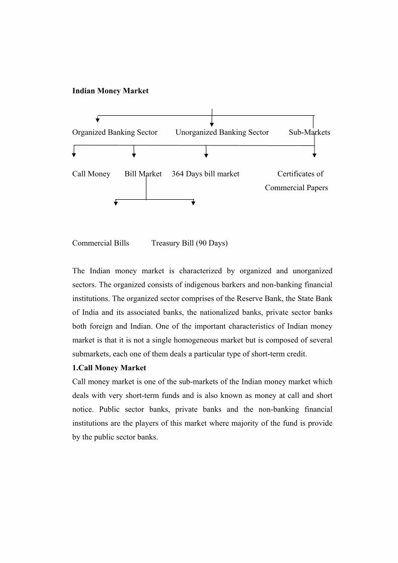
Indian Money Market

Organized Banking Sector Unorganized Banking Sector Sub-Markets

Call Money Bill Market 364 Days bill market Certificates of

Commercial Papers

Commercial Bills Treasury Bill (90 Days)

The Indian money market is characterized by organized and unorganized

sectors. The organized consists of indigenous barkers and non-banking financial

institutions. The organized sector comprises of the Reserve Bank, the State Bank

of India and its associated banks, the nationalized banks, private sector banks

both foreign and Indian. One of the important characteristics of Indian money

market is that it is not a single homogeneous market but is composed of several

submarkets, each one of them deals a particular type of short-term credit.

1.Call Money Market

Call money market is one of the sub-markets of the Indian money market which

deals with very short-term funds and is also known as money at call and short

notice. Public sector banks, private banks and the non-banking financial

institutions are the players of this market where majority of the fund is provide

by the public sector banks.

2.Bill Market in India

The bill market or the discount market is the most important component of the

money market where the short-term bills normally of 90 days are bought and

sold. The bill market is further divided into two parts namely commercial bills

and treasury bills. The government of India most often raises funds through 91

day treasury bills from the bill market.

RBI is the final authority and controller of monetary and banking conditions in

the country. It has the responsibility to guide and control the institutions of the

money market and to full fill this it is armed with both qualitative and

quantitative weapons of credit controls.

3.Features and Defects of the Indian Money Market

Presence of unorganized money market- one of the most alarming defect of the

Indian money market is the existence of the indigenous bankers, who do not

distinguish between short-term and long-term finance. They also are not guided

by the RBI guidelines and involve in all the ills of lending.

Lack of integration- A major defect of the Indian money market is the lack

of integration between different public sector, private and foreign banks. After

the passage of the Banking Regulation Act 1949 the problem of disintegration is

almost over.

Multiplicity of interest rates-Another defect of the Indian Money Market is the

existence of too many rates of interest which is due to the immobility of funds

from one section of the market to another.

Absence of the bill market- Indian Money Market did not have the bill market

whereas a well organized bill market is necessary for linking up the various

credit agency effectively to RBI.

Highly volatile call many market- This market is known for ‘money at call and

short notice’. It has in fact two segments - Call market or over night market and

short notice market. Call money market rates are determined by demand for and

supply of short term funds. Because money called for is always for urgent needs,

lending rates are always very much fluctuating ranging from 70% to 1.5% per

annum.

4. RBI and the Indian Money Market

R.B.I has been taking important measures time to time to remove the defects of

the Indian money market and it has been successful to a great extent too. The

discrimination between Indian and foreign banks does not exist now. Disparity

of interest rates from banks to banks on regional or sectional grounds does not

exist now. Through money market operations, shortages of money has also been

reduced considerably by the R.B.I.

5. The Reforms in the Indian Money Market

Recommendations of the Sukhmoy Chakravarthy Committee on the

review of the working of the Monetary system and the Narasimhan committee

report on the working on the Financial System in India,1991 have induced the

R.B.I to bring the series of money market reforms which is listed below:

Deregulation of Interest rates: R.B.I used to keep a strict control over interest

rates. But after the recommendation of Narasimham committee, interest rate

were further deregulated and financial institutions were freed to fix their rate of

interest.

R.B.I used to keep a strict control over interest rates but after the

recommendations of Narasimham committee interest rates were further

deregulated and financial institutions were freed to fix their rate of interest.

Introduction of new instruments in the money market-Previously there were

only 91 days treasury bills treaded in the money market but R.B.I introduced

new instruments like 182 days treasury bills, 364 days treasury bill, longer

maturity treasury bills, dated government securities, certificates of deposits and

commercial papers.

Traditionally 91 days Treasury bill has been an important instrument through

which the government of India raised funds for short periods and commercial

banks invested their short-term funds. There was a time when treasury bills by

commercial banks were solely governed by SLR Considerations. But the things

have changed now. They transact in the secondary market instrument also.

182 Days Treasury Bill

182 days treasury bills were variable interest bill and were sold through

fortnightly auctions. Though they were highly yield giving but they have been

replaced by 364 days Treasury Bills.

364 days Treasury Bills

Because of the success but difficult to operate 15 day treasury bill, there was

considerable scope for financial institutions to go for long-term bills. The 364

day treasury bills are important instruments of government borrowing form the

market. Financial institutions recognized the yield rate on 364 day treasury bills

as the anchor rate for floating interest rate instruments.

The R.B.I in 1997 introduced two more treasury bill that is 14 day intermediates

treasury bills and 14 day treasury bills.

Dated - Government Securities

The government of India has decided to sell dated securities that are 5 years

and 10 years maturity, on an auction basis. The purpose of which can be listed

as below:

To develop dated securities as a monetary instrument with flexible yields

For the financial instruments to suit investor’s expectations and

To meet the needs of the government directly from the markets.

Repos and Reverse Repos

Introduction of repos and reverse repos in 1992 is an interesting development in

respect of central government dated securities. Through these the R.B.I try to

bring the fluctuations in liquidity of the money market to minimum. Since 1996,

The R.B.I has introduced reverse repos that is to sell dated government

securities through auction at fixed cut of rate of interest. In the days the R.B.I is

using repos and reverse repos as a deliberate policy to influence the volume of

liquidity in the money market and also to stabilize the short term rate of interest

or the call rates. This policy of using repos and reverse repos is now called the

Liquidity Adjustment Facility (LAF) and this has emerged as a major instrument

of monetary policy since 2000-2001.

Certificates of Deposits(CDs)

The CDs are other important instruments of money market. Initially,

CDs were issued in the multiples of Rs 25 lakhs but it was reduced to Rs 1 lakhs

to increase the investors’ base. The maturity is between 3 months and one year.

They are issued at a discount rate and that is freely determined according to

market conditions. CDs are freely transferable after 45 days from the date of

issue.

Commercial Paper(CP)

The commercial papers are issued by companies of a net worth of Rs.5 crore.

This is issued in the multiples of Rs 25 lakhs subject to a maximum issue of Rs

1 crore. The maturity period subject of a commercial paper is between 3 to 6

months. They are issued at discount rate, the face value which is freely

determined. Maximum amount of CP that a company can raise is limited to 30%

of the maximum permissible bank finance. The purpose of introducing CP is to

enable high level corporate borrowers to diversify their source of short-term

borrowing on the one hand, and provide an additional instrument to the banks

and financial institutions in the money market, on the other.

Summary

Finance in broader sense, refers to monetary resources needed by individuals,

industries, business houses, farmers and government to carry out their activities

smoothly. The whole finance system in India is classified as – agricultural

finance, industrial finance, development finance and government finance. Study

of this lesson enables us to know the structure, components, organization and

characteristics of Indian money and capital market. Indian money market is

comprised of organized banking sector, unorganized banking sector and sub

markets which in itself is comprised of call money market, bill market, 364 days

bill market certificate of deposits, commercial papers. The bill market is of two

types – commercial bills and treasury bills. Indian money market has many

defects like – presence of unorganized money market, lack of integration,

multiplicity of interest rates, absences of bill market, highly volatile money

market. The Reserve Bank of India has brought many reforms in the Indian

money market.

Review Question and Keys.

Explain the meaning and structure of Indian money market.

(Refer to the introduction of this lesson and sub point 1 – composition of Indian

money market.)

Explain the reforms in Indian money market.

(Refer to sub point 5 of this lesson)

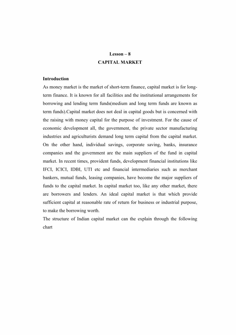
Lesson – 8

CAPITAL MARKET

Introduction

As money market is the market of short-term finance, capital market is for long-

term finance. It is known for all facilities and the institutional arrangements for

borrowing and lending term funds(medium and long term funds are known as

term funds).Capital market does not deal in capital goods but is concerned with

the raising with money capital for the purpose of investment. For the cause of

economic development all, the government, the private sector manufacturing

industries and agriculturists demand long term capital from the capital market.

On the other hand, individual savings, corporate saving, banks, insurance

companies and the government are the main suppliers of the fund in capital

market. In recent times, provident funds, development financial institutions like

IFCI, ICICI, IDBI, UTI etc and financial intermediaries such as merchant

bankers, mutual funds, leasing companies, have become the major suppliers of

funds to the capital market. In capital market too, like any other market, there

are borrowers and lenders. An ideal capital market is that which provide

sufficient capital at reasonable rate of return for business or industrial purpose,

to make the borrowing worth.

The structure of Indian capital market can the explain through the following

chart

Capital Market in India

Govt. Securities Industrial securities Development Financial Financial

(guilt edge market) Market Institutions Intermediaries

New Issue Market Old Issue Market

(Stock Exchange)

IFCI ICICI IDBI IIBI UTI

Merchant Banks Mutual Funds Leasing Companies Venture Capital Others

companies

Objectives

Study of this lesson will enable the students to know the structure, functioning,

organization and control mechanism of the Indian capital market. They will also

be in a position to make an analysis of the role of SEBI in bringing a level

playing field in the capital market.

Guilt-edge Market:

The guilt edge market is referred to the market for the government and semi

government securities, backed by Reserve Bank of India. The value of the

securities traded in this market is stable and are much sought after by banks and

other institutions.

Industrial Securities Market:

Industrial securities market refers to the market for shares and debentures of old

and new companies. This is also known as new issue market and old capital

market which means stock exchange. The new issue market also known as

primary market deals in rising of new capital in the form of shares and

debentures. The old issue market or the stock exchange deals in securities

already issued by companies.

Both the markets-primary and secondary or new issue and old issue market- are

necessary but the primary market is more important with respect to economic

development.

Development Financial Institutions

The Government of India, soon after the independence, set up a number of

financial institutions to facilitate the private sector industries for providing

finance to them as a view to speedy economic development of the country. The

first financial institution setup in this regard was IFCI(1948). Next was SFCs,

which were setup by state governments with the cooperation from the Reserve

Bank of India, to provide long and median finance to median and small scale

industries. ICICI, IDBI, UTI were established in the years 1955, 1964 and 1964

respectively. The LIC was setup in 1956 to mobilize saving from the individuals

and to invest a part of it in the capital market. Apart from these, many other

special institutions were setup for the above mentioned purpose and they are

popularly known as public sector financial institutions. The development

financial institutions provide funds to the private sector enterprise. They have

been doing a tremendous job, is evident in the manner that while in 1970-71 to

total assistance by these institutions stood at Rs.203 crores, increased up to an

unimaginable amount of Rs.1,21,350 crores in 2000-2001.

Bank and the Capital Market

Commercial banks are one of the most important organs of the Indian capital

market but they have restricted their operations to the purchase and sale of

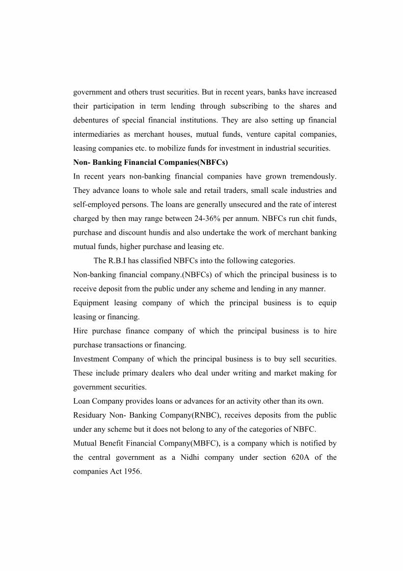
government and others trust securities. But in recent years, banks have increased

their participation in term lending through subscribing to the shares and

debentures of special financial institutions. They are also setting up financial

intermediaries as merchant houses, mutual funds, venture capital companies,

leasing companies etc. to mobilize funds for investment in industrial securities.

Non- Banking Financial Companies(NBFCs)

In recent years non-banking financial companies have grown tremendously.

They advance loans to whole sale and retail traders, small scale industries and

self-employed persons. The loans are generally unsecured and the rate of interest

charged by then may range between 24-36% per annum. NBFCs run chit funds,

purchase and discount hundis and also undertake the work of merchant banking

mutual funds, higher purchase and leasing etc.

The R.B.I has classified NBFCs into the following categories.

Non-banking financial company.(NBFCs) of which the principal business is to

receive deposit from the public under any scheme and lending in any manner.

Equipment leasing company of which the principal business is to equip

leasing or financing.

Hire purchase finance company of which the principal business is to hire

purchase transactions or financing.

Investment Company of which the principal business is to buy sell securities.

These include primary dealers who deal under writing and market making for

government securities.

Loan Company provides loans or advances for an activity other than its own.

Residuary Non- Banking Company(RNBC), receives deposits from the public

under any scheme but it does not belong to any of the categories of NBFC.

Mutual Benefit Financial Company(MBFC), is a company which is notified by

the central government as a Nidhi company under section 620A of the

companies Act 1956.

Miscellaneous Non Banking Company(MNBC) manages, conducts and

supervise chit funds.

There is no specific legislation to government the NBFCs instead they come

under there different agencies. There are-

NBFCs are governed by the companies Act 1956 because they are limited

liability companies and they don’t even come under the definition of a finance

company.

With regards to its deposit, NBFCs are governed by Non Banking Financial

Companies(Reserve Bank) Directions 1997.

Some of the NBFCs are governed by SEBI who are engaged in merchant

banking and portfolio management.

But the government of India enacted the Reserve Bank of India (Amendment)

Act, 1997, which confers wide ranging powers on R.B.I for controlling the

functioning of non banking financial companies.

Merchant Banking

The concept of merchant banking is relatively new in India in the area of

financial services. It caters to the needs of trade and industry by acting as

intermediary, consultant, financial and liaison agency initially, commercial

banks setup merchant banking divisions, which later became separate merchant

banking subsidiaries. Merchant banks in India manage and underwrite new

issue, undertake syndication of credit, they advise corporate clients on fund

raising and other financial aspects. They don’t under take banking business like

deposit banking, lending and foreign exchange services like foreign merchant

banks.

The merchant banks in India were subject to two types of authorities-

1. The SEBI( The Securities and Exchange Board of India ) sought to authorize

and regulated all merchant banks on issue activity and portfolio management of

their business and ,

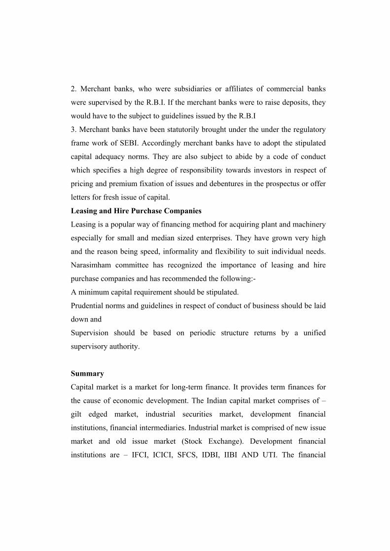
2. Merchant banks, who were subsidiaries or affiliates of commercial banks

were supervised by the R.B.I. If the merchant banks were to raise deposits, they

would have to the subject to guidelines issued by the R.B.I

3. Merchant banks have been statutorily brought under the under the regulatory

frame work of SEBI. Accordingly merchant banks have to adopt the stipulated

capital adequacy norms. They are also subject to abide by a code of conduct

which specifies a high degree of responsibility towards investors in respect of

pricing and premium fixation of issues and debentures in the prospectus or offer

letters for fresh issue of capital.

Leasing and Hire Purchase Companies

Leasing is a popular way of financing method for acquiring plant and machinery

especially for small and median sized enterprises. They have grown very high

and the reason being speed, informality and flexibility to suit individual needs.

Narasimham committee has recognized the importance of leasing and hire

purchase companies and has recommended the following:-

A minimum capital requirement should be stipulated.

Prudential norms and guidelines in respect of conduct of business should be laid

down and

Supervision should be based on periodic structure returns by a unified

supervisory authority.

Summary

Capital market is a market for long-term finance. It provides term finances for

the cause of economic development. The Indian capital market comprises of –

gilt edged market, industrial securities market, development financial

institutions, financial intermediaries. Industrial market is comprised of new issue

market and old issue market (Stock Exchange). Development financial

institutions are – IFCI, ICICI, SFCS, IDBI, IIBI AND UTI. The financial

intermediaries are like – Merchant Banks, Mutual Funds, Leasing Companies,

Venture Capital Companies and others.

Review Question and Key

1. Explain the meaning and components of Indian capital market

(Refer the introduction of this lesson)

2. Explain merchant banking and leasing and hire purchase companies

(Refer to merchant banking and leasing hire purchasing companies in this

lesson)

Lessons – 9

MUTUAL FUNDS

Introduction

The orgin of the mutual funds can be traced in Britian in the late 19th century

and early 20th century. Unit trust was the first mutual fund in India which was

set up in 1964. Mutual funds are those who represent pooled savings of investors

in divesified portfolio to obtain maximum return on investment with the

minimum risk. In recent years, mutual funds have become most important

among the newer capital market inistituions. Like unit trust of india, many

public sector banks and financial institutions have setup mutual funds on tax

saving schemes.

Objectivies of Mutual Funds

To provide investment opportunity to the small investors to participate in the

fast growing corporate securities market through indirect way.

To provide a higher return than the banks without having much risk.

To mobailize savings from the small investors and channalise than for productive

purposes.

To provide multiplicity of investment options like current return, capital appriciation,

tax benefit or a combination of all these.

To strengthen the capital market by assuring better flow of funds.

Contents

Meaning of mutual funds

Objectives of mutual funds

Registration and Trustee

Advantages of mutual funds

SEBI’s regulations

Some Major Private Mutual Funds

ICICI Ltd. Mutual Fund, IDBI Mutual Fund, Kothari Pioneer Mutual Fund, 20th

Century Mutual Fund, Alliance 1995, GIC Mutual Fund, Birla Mutual Fund, JM

Mutual Fund and ITC Mutual Fund etc.

Government allowed the entry of mutual fund in 1992 and SEBI has

cleared a number of private mutual funds. Above mentioned are a few among

them.

Registration and Trustee: Mutual funds are required by law to obtain a

certificate of registration from the SEBI. They have to apply in form A and

deposit a fee of Rs. 25000/-. A mutual fund will be constituted as a trust under a

registered trust deed and managed by a trustee or by a board of trustees.

Advantages of Mutual Funds

Safety and stable return.

Convenience in investment. Investors need not worry where to invest.

Since it is invested in different portfolios, risk factor is reduced tremendously.

Broad basing of capital and the benefit of professional and skilled fund

management.

It helps speedy formation of capital in the country.

Even small and pawn sophisticated investors are benefited by the mutual fund.

Freedom of selection from wide range of schemes having excellent liquidity.

SEBI’S Regulation

SEBI is empowered to lay guidelines and supervise and regulate the functioning

of mutual funds. The guidelines will include advertisements, disclosures and

reporting requirements. Mutual funds are under obligation to inform the

investors regarding the status of their investment in equities, debentures and

government securities. SEBI has introduced uniform regulations for the mutual

funds in the country, known as SEBI(Mutual Funds) Registration, 1993 which

comprises of the following guidelines.

Mutual funds has to be established as a trust and should be managed by a

separate asset management company(AMC). Mutual funds should be supervised

by board of trustee.

The AMC must have a minimum net worth of Rs.6 crores of which the sponsors

must contribute at least 40 percent.

Approval of SEBI must be obtained for the offer documents of scheme of

mutual funds.

SEBI prescribe the minimum amount should be raised by each scheme.

The norms of advertisement and truthful discloser by the mutual funds in

advertisements and publicity materials. (Incomplete sentence.)

Summary

Britain is the mother land of mutual fund. In India, Unit Trust was the first

mutual fund which was set up in 1964. Mutual funds are those who represent

pooled savings of investors in diversified portfolios to obtain maximum return

on investment with the minimum risk. The main objectives of the mutual funds

are like providing opportunities the small investors to participate in securities

market, to provide higher return than the banks, to mobilize savings from small

investors, to provide diversified investment portfolios and strength and capital

market. By now private mutual funds are also allowed to participate in the

capital market. Some of them are like ICICI Ltd. Mutual fund, IDBI Mutual

Fund, Kothari Pioneer Mutual Fund etc. There many advantages of mutual funds

as safety of investment, stable returns convenience, minimum risk and high

return etc. SEBI regularizes the function of mutual fund.

Review Questions and Key

1) Explain what is a mutual fund.

(Refer to the introduction of this lesson)

2) What are the objectives of mutual fund?

(Refer to the objective part of this lesson)

3) Account for the advantages of mutual funds.

( Refer to the advantages part of this lesson)

4) Explain and comment on the various guild lines of SEBI for the regulation

of mutual funds.

(Rrefer to the SEBI regulation part of this lesson)

Lesson – 10

VENTURE CAPITAL FUNDS

Introduction

There are occasions when small entrepreneur fail to convince the banks to

finance for their small enterprises and therefore they fail to get finance. In these

situations some big and giant business organization, come forward to help these

numerous small enterprises by providing seed and growth capital. OECD has

defined the venture capital in the following words Capital provided by forms

who invest along side management in young companies that is not quoted on the

stock market. The objective is high return form the investment. Value is created

by the young company in partnership with the venture capitalists money a

professional expertise. The importance of venture capital companies is to give

commercial support to new ideas and for the introduction and adaptation of new

technologies. It also involves a very high degree of risk in financing venture

capital.

Objectives

To understand the mechanism of venture capital cycle.

To know the over all scenario of venture capital in India

Contents

a) Current trends in India.

b) Venture capitalist

c) Benefits of the venture capital.

d) Narasimham committee’s views

Current Trends in India

After the Government of the India Guidelines in 1988, many new venture capital

funds were sponsored in India. ANZ Grindlays bank, an American bank, setup

the first private venture capital fund. It was called ‘India investment fund’ there

after a number of foreign and indigenous funds came in the field. Now a

situation has come where capital is pouring into private equity funds. The

average ticket size of venture capital is also increasing. The small investors or to

say the first entrants entrepreneurs are finding easier to raise fund. Many state

governments are also setting regional venture capital funds competitions in

stretching the valuation and there by V.C. firms are focusing the specific

industries.

The flow of venture capital from in the investor to a start-up company and back

passes through-

(a). Rising of venture fund,

(b).Investing in, monitoring of and adding value to firms and

(c) Existing successful companies returning capital to investors.

Venture Capitalist

A venture capitalist is that who is a wealth man and finance to start-up

companies. The start-up companies are normally new entrants or innovators who

do not get financed by the banks for his or her newly developed product.

Venture capital and private equity firms are pools of capital who are typically

organized as a limited partnership. They invest in companies that provide an

opportunity of high rate of returns within five to seven years. They will properly

investigate about the opportunities in several such firms and then invest. Venture

capitalists are not simply the passive financiers, but they foster growth in

companies through their involvement in the management, strategic marketing

and planning of their investee companies. Therefore, they are normally called as

entrepreneurs first and financiers next.

There are different size of venture capital firms from small seed

specialist firms of a few crores of rupees to several hundred and thousand of

crores of rupees.

Benefits of Venture Capital

It has been experience that companies financed and baked by venture capitalist

have grown faster than other type of companies. This became possible because

of active involvement of experienced and expert venture capitalist.

Most often it becomes a challenge for the venture capitalist to see that the

company earns profit and thus they do not leave any stone unturned.

The venture capital firms will try to increase a company’s value to its owners,

without taking day to day management control.

Venture capital firms usually work in tandem with other financiers and they may

be able to help the entrepreneurs to put a total funding package together for the

benefits of the entrepreneurs.

NARASIMHAM Committee’s Views

The Narasiham committee was of the opinion that the guidelines for

the setting up of venture capital companies were too stringent and unrealistic

and thus be relaxed. Since venture capital is associated with high rise factor, the

committee recommended a reduction in tax on capital gains made by this

companies and equality of tax treatment between venture capital companies and

mutual funds. The central government launched the National Venture Fund for

Software and IT industry (NVFSIT) to provide funds for technology

development particularly for small and medium industries. It is managed by

SIDBI( Small Industries Development Bank of India) SEBI has been made the

single point nodal agency for registration - and regulation of both domestic and

overseas capital funds.

Infrastructure Leasing and Financial Services Ltd.(IL&FS)

Infrastructure leasing and financial services Ltd. was set up in 1988,

which focuses on leasing of equipment and infrastructure development. The

company has been specially directed for structuring the finances of major

projects in the power and transportations sector since in 1994-95, IL & FS has

made a remarkable success in commercialization of infrastructure projects. In

association with the various states and central government agencies, it has

worked for developing infrastructural projects in railways, power generation,

telecommunication, water supply, water transport system etc. It is also engaged

in the fields of investment banking and undertakes merchant banking activities.

IL & FS is actively engaged in money and gilt-edge markets for trading in

government securities, bonds of public sector undertakings, corporate

debentures and units.

Summary

When the small and new entrants in the business and industries, having failed to

convenience to banks of the gains form their prospective projects some of the

wealthy people come forward to finance them with the seed and growth capital.

This is known as venture capital and those who provide finance are called

venture capitalist. After 1988 government guidelines, many new venture capital

funds were sponsored in India. ANZ Grindlays Bank was the first private

venture capital fund in India. There are many benefits of venture capital like –

venture capital finance companies grow fast, venture capitalist take it as a

challenge profit making of the companies, etc.

Review Question and Key

What is venture capital and who is a venture capitalist?

(Refer to the introduction and venture capitalist headlines of this lesson)

Explain the benefits of Venture Capital. Discuss Narasimham committee’s

views on venture capital

(Refer to the headlines - benefits of the venture capital and Narashimam

committee’s views)

Lesson – 11

CREDIT RATING

Introduction

With the development of finance market, number of institutions started

operating in a very tough competitive atmosphere and thus, many companies

came out with varied and attractive investment schemes. To invest an investor

must assure himself of all the risks involved and therefore, the need was felt to

have credit rating agencies that should work independently and rate the

companies. America is the mother of credit rating where it was introduced in

1909. Credit rating is a codified rating assigned to an issue by authorized credit

rating agencies like CRISIL, CARE and ICRA extra. These agencies have been

promoted by well established financial institutions like IDBI, ICICI, UTI etc.

Credit rating is a relative raking through a systematic analysis of the strengths

and weakness of a company based on financial statement project analysis,

credit-worthiness etc.

Objectives of Credit Rating

Credit rating has the following objectives:-

1) To provide a better information to the investors.

2) To provide the investor a sound basis for proper risk - return structure.

3) To teach the borrower a healthy discipline.

4) To assist in framing the guidelines for public policy on institutional

investment.

Contents

Credit Rating agencies in India.

Rating methodology.

1. Credit Rating agencies in India

The need for credit rating agencies has been in discussion in recent time in India

and after being convinced about its need, the first credit rating agency which

was established in India was the Credit Rating and Information Services of India

Ltd. (CRISIL) in 1987, since then, there has been a rapid growth of credit rating

agencies in India. The major credit rating agencies in India are- CRISIL,

Investment information and credit rating agencies of India Ltd.(ICRA), and

Credit Analysis and Research Ltd(CARE) etc.

2. Rating Methodology

The process of rating starts with the company approaching the rating agency for

rating. The experts are given a free hand and they collect data and information.

Then they investigate strengths and weaknesses of the business in detail. The

entire process of investigation and analysis are kept top confidential. The key

factors which are generally examined are:-

Business analysis, Economic analysis, Industry analysis, Financial

analysis, Management evaluation, Geographical analysis and Fundamental

analysis etc.

Summary

With a very high pace of development of financial market, a number of

institutions started operating in a highly competitive condition. Many companies

came with varied and attractive investment schemes. For the small investors it

became difficult to know the credit worthiness of this institution. That is why the

need for credit rating was felt. Credit rating agencies provided better information

to the investor and the borrower a healthy discipline.

Review Question and Key

Explain the objectives and importance of credit rating.

(Mention the contents in this lesson)

Lesson – 12

STOCK EXCHANGE IN INDIA

Introduction

Stock exchange or the secondary market is that where purchase and sale of

shares are affected in a free market conditions. The joint stock companies or

corporate houses issue stock and bounds and enables those who have surplus

funds to invest them profitably in either of them according to their choice. A

Stock exchange is an association of member brokers for self regulating and

protection of their interests.

The first stock exchange in India was started in Bombay in the year 1875

in the name of Native Share Stock Brokers Association and later it became

popular by the name of Bombay Stock Exchange.

Objective

By reading this lesson the students would be in a position to understand the

meaning, objectives, Features and the functioning of the stock exchange in

India.

Contents

Regulation which governs stock exchange-

Organization-

1 Role of stock exchanges-

2 Qualification for membership-

3 Process of Transaction-

4 SEBI and Capital Market Reforms.

Regulation for Governing Stock Exchange

the SC(R) Act 1956 and the securities contracts (regulation) rules 1957 regulate

certain matters of trading on stock exchanges subjects like opening and closing

of the stock exchanges, timing of trading, banks transfer regulation, bank

regulation, badla regulations, settlement, fixation of margin, market prices,

regulation of broker trading, brokerage charges, trading rules etc are governed

by the bylaws of the exchanges.

Organization

On the organization front stock exchanges in India are divided into two

categories.

Non profit making and

Profit making exchanges

Stock exchanges at Mumbai, Ahemadabad, Indore are voluntary non-

profit making associations, while Kolkata, Dehli, Banglore, etc. are joint stock

companies limited by shares. There is uniformity in their organization because

the Rules of Articles of association which defines the constitutions of the

recognized stock exchanges are approved by the Central Government.

The decision making body of the stock exchanges is a governing body which

has wide governmental and administrative powers. Subject to the approval of the

government, it can make, amend and suspend the operation of the rules, bylaws

and regulations of the exchanges. The constitution has provided it absolute

power of jurisdiction over all members, power of management and control. The

constitution also provides it the power to and admits expel members, to warn,

censure, fine and suspend, members and their partners etc. It has also the power

to determine the mode and conditions of the stock exchange business and to

supervise direct and control all matters and activities affecting the stock

exchange.

The organization of Mumbai exchange is different. The members elect

16 directors for the Governing board. The governing board elects a President, a

Vice- President and a treasurer. The governing board recommends the name of

the Executive Director to the government. There are three representatives from

the government, three from the public and one from the RBI.

Role of stock Exchanges: In a capitalistic system companies and corporate

houses depend upon stock exchanges for raising funds. For that purpose the

companies have to get listed in the stock exchanges. Stock exchanges provide

liquidity to the listed companies. Its role and function can be listed as follows:

1. This provides a market place for purchase and sale of securities. It ensures

free transfers of securities which is the essential basis for the joint stock

enterprise system. This is why the private sector companies fully depend on

stock exchange for market their securities.

2. It provides linkage between household savings and investment in the

corporate economy.

3. It also provides market quotations of the prices of shares and bonds. It makes

a stock exchange the provider of input for predicting economic trend.

4. The stock exchanges in India serve the joint sector units as also to some

extent public sector enterprises.

5. Stock exchanges in India provide a market for gilt - edge securities.

Qualification for Membership

A person should full fill the following conditions for becoming a member of a

recognized stock exchange-

i) Should be an Indian citizen.

ii) Must be of 21 years of age.

iii) Should not have compounded with creditors.

iv) Must not have been convicted for fraud or dishonesty.

v) Should be engaged as agent or broker only.

vi) Should not be a defaulter or of any other stock exchange.

vii) Should work at least for two years in any capacity as a member.

Process of Transaction: The investment transaction passes through following

four stages-

Exchange of the Order: A Clint places his order to a stock broker who is

entitled to do business in a stock exchange.

Execution of the order:- After placing the order , the broker or his clerk will

execute the order and that will appear in the stock exchange daily official list

showing the number and price of shares

Reporting the tail to the Clint:- The moment the deal is transacted, the broker

will send a contract note to the client giving details of the security bought or

sold, prices and broker’s commission etc.

Settlement of Transaction- In the case of cash transaction, payment has be made

immediately on the transfer of the securities, or within a period of one to seven

days. But in case of forward delivering contracts, the settlement is made on a

fixed day generally a fortnight.

The National Stock Exchange

India in the recent past has witnessed wide ranging changes in its economy and

its organs. Stock market is one of them. Liberalization and Globalization are the

mantras of the day. The setting of the National Stock Exchange is an important

part of the securities market reform process of the country. Though securities

trading is not a new phenomenon in India but it was not keeping pace and

standard as per the requirement of the day because securities trading in India

was experiencing multiplicity of defects as lack of trading facilities with fairness

and accessibility and dated procedures and long and uncertain settlement cycles.

1980’s is a land mark with regards to the growth of capital market in India. It

witnessed a manifold increase in the number of companies, investors, brokers,

and stock exchanges. Mr. M.J.Pherwani the Chairman of the Expert Group

recommended the establishment of the National Stock Exchange .Hence, the

National Stock Exchange came into existence in November 1992 with an equity

capital of Rs. 25 crores but started its operation in November 1994.Companies

with capital of Rs. 10 crores are eligible for listing .The NSE has been

established for providing a nation wide stock trading facility and will operate in

traditional and non traditional market for equities.

The NSE has the following objectives:-

1.To provide a nation wide trading facility for trading in equities, debt and

hybrids.

2.It provides equal access to the investors across the country.

3.To ensure fairness, efficiency and transparency in security trading.

4.To ensure shorter settlement cycles.

5.To provide international standard in the trading of securities.

Functioning of the NSE

National Stock Exchange has a nation wide network for providing trading

facilities and equal access to investors across the country. There is no trading

floor and each trading member has to have a computer in his office. This

computer will be linked to the central computer at the NSE by internet. Thus it

provides a high tech trading facility. The trading system provides a high

flexibility to trading members. They can easily exercise the various options

which are traditionally available to them on trading floor. When entering the

order a trading member is empowered to place various conditions on the order.

The system provides complete transparency. The identity of the trading

members is kept secret and revealed only on confirmation of a trade to the

respective counter parties. When securities are sold and delivery made to the

clearing system, they are transferred to a depository. Each trading member is

provided a pass book showing securities deposited by the trading member.

Every client of the trading member has to have a sub account where records of

share holding of the client will be maintained .The pass book of the trading

member is updated through electronic book entry method every time the

transaction is made.

SEBI and Capital Market Reforms

SEBI (the Securities and Exchange Board of India) was set up in 1988 as a non

statutory body to regulate the functioning of the capital market which was

suffering from the weakness like- long delays, lack of transparency and

vulnerability to price rigging and insider trading. It was made a statutory body in

1992. SEBI was authorized to regulate all merchant banks on issue activity,

regulate and supervise the working of the mutual funds and also to over see the

functioning of the stock Exchanges in India. In constitutions with the

government, SEBI has introduced a number of steps to improve the functioning

of the Stock-Exchange in India.

On the recommendation of the Narasimham committee, the

government of India abolished the post of Control of Capital Issues (CCI) and

instead, SEBI was given the power to control and regulate the new issue market

as well as the old issue market.

Primary Market Reforms

SEBI has issued various guidelines for the issue of capital. Companies now have

to disclose material facts and risks factors with their projects. And the basis of

fixing premium. Not only that, SEBI has also introduced a code of

advertisement for public issues for the purpose of fair and truthful disclosures.

For reducing cost of issue, understanding of issue has been made optional

subject to certain conditions. It has raised the minimum application size,

regulated acquisition and takeover etc. Merchant banking gas been statutorily

brought under the regularity frame work of the SEBI. Since 1992, the

government of India allowed Indian companies to access international capital

markets through Euro equity shares.

Secondary Market Reforms

Under the provision of Securities and Stock Exchange Board Act, 1992, SEBI

has started registering the intermediaries like stock brokers and sub-brokers.

While registering SEBI will adequacy, infrastructure etc. It has also notified

regulation an insider trading. It has amended the organization of the governing

body also and by now the governing body must have 5 elect members, not more

than government nominated as public representatives. The government has

allowed Foreign Institutional Investors (FIIs) to invest in the Indian capital

market provide they are registered with the SEBI. Till January 1995, as many as

286 FIIs have been registered with the SEBI. To prevent excessive speculation

and volatility in the stock market, SEBI has introduced rolling settlement from

July 2002, under which settlements has to be made every day.

Reforms in the Insurance Sector

After a wide range of reforms in the capital market it was felt necessary to bring

reforms in the insurance sector also. Accordingly in the year 1999-2000 the

Insurance Regulation and Development Authority Act was passed despite stiff

opposition from trade unions and left parties. The IRDA Act brought an end to

the monopoly of the government in the insurance sector because it aims to

promote private sector including foreign companies, in the insurance sector. It

provides priority for the utilization of the policy holder’s funds in infrastructure

development. So far the government has given the licenses to a number of

private sector companies to participate in this business.

Wide ranging powers to SEBI for better functioning of the Capital Market

In the due course the government of India felt that SEBI should be strengthened

more specially after experiencing Security Scam (Popularly known as Harsad

Mehta Scam) in early 90’s.Accordingly in January 1995, the Government of

India promulgated an ordinance to amend SEBI Act 1992 so as to empower

SEBI with additional powers for ensuring the orderly development of the capital

market and to enhance its ability to protect the interests of the investors.

Important clauses of this ordinance are:

To enable SEBI to respond quickly to market conditions and to reinforce its

authority, it can go to the courts without prior approval of the government

matters related to any dispute.

SEBI is now provided with the regulatory powers over companies in the

issuance of capital, the transfer of securities and other related matters.

SEBI can now impose monetary fine on capital market intermediaries and other

participants for a listed range of violations.

SEBI can now summon the attendance of and call for documents from all

categories of market intermediaries, including persons from the securities

market.

Summary

Stock exchange or the secondary market is that where sale and purchase of

shares are perfected in a free market condition. The joint stock companies and

corporate houses issue stock and bonds in this market. The first stock exchange

of India was started in Bombay In the year 1875 in the name of Native Share

Stock Brokers Association.

Stock exchanges of in India are divided into two categories – a) Non

profit making and b) Profit making exchanges. To become member of the stock

exchange a person has to full fill certain conditions. The process of transaction

consists of – exchange of the order, execution of the order, reporting the deal to

the client and settlement of the transaction. SEBI has brought the reforms in

both the markets – primary market and secondary market.

Review Question and Key

1. Explain the organization and role of stock exchanges in India.

(mention the sub point 2 and 3 of the lesson)

2. Explain the qualification for membership and reforms in the capital

market.(mention the contain explain under the sub points 4 and 6 of the lesson)

GLOSSARY OF WORDS

Accounting Rate of Return: It is calculated by dividing the average annual

profit by the average investment. The concept is used in project evaluation or

capital investment decisions.

Aggregate demand: It is the sum of all planned consumption, investment,

government purchases, and net exports.

Aggregate Demand Schedule: A schedule showing the inverse relationship

between the general price level and aggregate demand.

Aggregate Supply schedule: It is a schedule showing the relationships between

the general price level and the volume of real goods and services business firms

supply to the product market.

Aggregate Supply: The total volume of real final goods and services provided by

business to the market.

Appreciation: An increase in value.

Arc Elasticity of Demand: The price elasticity of demand between two points on

the demand curve.

Arc Elasticity of Supply: The price elasticity of supply between two points on

the supply curve.

Autonomous consumption: The minimum level of consumption independent of

the Level of disposable income.

Autonomous investment: Investment independent of level of income and the

state of the economy.

Average Fixed Cost (AFC): Total fixed Cost divided by output i.e. fixed cost per

unit of output.

Average Product (AP): The total product divided by the quantity of the variable

factor used.

Average propensity to consume: The fraction of income that is spent on

consumption goods.

Average propensity to save: The fraction of income that is saved.

Average revenue (AR): Total Revenue divided by the quantity sold.

Average Total Cost (ATC): Total Costs divided by output.

Average Variable Cost (AVC): Total variable Cost divided by output.

Balanced Budget: A budget in which total revenues and total expenditures are

equal.

Balance of Payments: The difference between a country's payments to foreigners

and its receipts from the foreigners.

Barter: The direct exchange of goods and services without the use of money.

Break-Even point: The point at which total revenues equal to total costs.

Business Cycles: The periodic fluctuations in economic activity.

Capital: A produced means of further production.

Consumption function: The relationship between income and consumption.

Discount rate: The rate at which cash flows are discounted.

Economic Cost: It is the explicit cost as per accounting records and the implicit

cost which is opportunity cost.

Economics: It is a branch of social science dealing with the allocation of scarce

resources among alternative uses to satisfy human wants.

Factors of Production: Those factors that are used in production like land,

labour, capital and organization.

Fiscal Policy: the financial policy of the government dealing with government

expenditure, taxes, or transfers used for stabilizing the economy.

Forecasting: Predicting future value of a variable on the basis of current and past

trend.

Gross National Product (GNP): The total market value of all final goods and

services produced by an economy in a year.

Imports: The purchase of goods produced abroad by any country.

Isocost: Different combinations of two inputs that a firm can purchase with the

same amount of money represented in a curve.

Isoquant: Different combinations of two inputs that produce the same level of

output represented in a curve.

Long Run: The time period when all inputs can be varied.

Marginal Cost: The incremental change in total cost by producing one more

unit.

Marginal Revenue: The incremental revenue in total revenue by selling one

more unit.

Merger: The combining of two or more firms under one ownership.

Monetary Policy: The policy of the Central Bank to stabilize the economy by

changes in money supply.

Monopoly: The market situation where there is only one producer or seller.

Normal Profit: The profit at total cost and total revenue are equal.

Oligopoly: A market situation in which there are only few producers or sellers.

Penetration Pricing: A pricing policy in which a lower price is charged than

economically feasible to penetrate in to the market.

Product Market: The Market in which real goods and services are bought and

sold.

Profit: The reward for entrepreneurship after payment of wages, rent and

interest.

Quota: A quantitative restriction on the value or volume of imports or exports.

Recession: A period of lower level of economic activities when unemployment

increases.

Rent: The return received for the use of real property.

Saving: The part of disposable income that is not consumed.

Short Run: A short period of time when at least one input is fixed.

Tax: A compulsory payment levied by a government without ensuring any

particular service.

Total cost: Total fixed cost plus Total variable cost.

Uncertainty: The state in which decision makers do not know the possible

outcome of their decisions.

Utility: The ability of goods to satisfy a want.

Value addition: The increment to the value of an item when it passes through

each stage of production process.

Yield: The return on an investment.

Glossary of Abbreviations

1. CSO – Central Statistical Organization.

2. ICICI – Industrial Credit and Investment Corporation of India.

3. IFCI - Industrial Finance Corporation of India.

4. IRBI - Industrial Reconstruction Bank of India.

5. EXIM-BANK – Export Import Bank

6. SFCs – State Financial Corporations

7. SIDCs - State Industrial Development Corporation.

8. IDBI - Industrial Development Bank of India.

9. UTI - Unit Trust of India.

10. NBFCs – Non- Banking Financial Companies.

11. SEBI – Securities and Exchange Board of India

12. AMC – Asset Management Committee.

13. NVFSIT- National Venture Fund for Soft Ware and Information

Technology.

14. IL & FS Ltd. Infrastructure Leasing and Financial Services Limited.