unit1: elements of digital communication...
TRANSCRIPT

Digital Communications
Unit1: Elements of digital communication system 1) Advantages of digital communication systems
Advantages and Disadvantages of Digital Communication Advantages:
1. Because of the advances in digital IC technologies and high speed computers, digital communication
systems are simpler and cheaper compared to analog systems.
2. Using data encryption, only permitted receivers can be allowed to detect the transmitted data. This is
very useful in military applications.
3. Wide dynamic range is possible since the data is converted to the digital form.
4. Using multiplexing, the speech, video and other data can be merged and transmitted over common
channel.
5. Since channel coding is used, the errors can be detected and corrected in the receivers.
Disadvantages:
1. Because of analog to digital conversion, the data rate becomes high. Hence, more transmission
bandwidth is required for digital communication
2. Sampling theorem
Statement: A continuous time signal can be represented in its samples and can be recovered back
when sampling frequency fs is greater than or equal to the twice the highest frequency component of
message signal. i. e.
Proof: Consider a continuous time signal x(t). The spectrum of x(t) is a band limited to fm Hz i.e. the
m.
s.
The output of multiplier is a discrete signal called sampled signal which is represented with y(t) in the
following diagrams:

Digital Communications
Here, you can observe that the sampled signal takes the period of impulse. The process of sampling can be
explained by the following mathematical expression:
3. PCM generation and reconstruction
Pulse-code modulation or PCM is known as a digital pulse modulation technique. In fact, the pulse-code
modulation is quite complex as compared to the analog pulse modulation techniques i.e. PAM, PWM and
PPM, in the sense that the message signal is subjected to a great number of operations.
Fig.1 shows the basic elements of a PCM system .

Digital Communications
c) : Receiver
Fig.1 : The basic elements of a PCM System
It consists of three main parts i.e. ,
Transmitter
Transmission path
Receiver
The essential operation in the transmitter of a PCM system are :
Sampling
Quantizing
Encoding
The human voice uses frequencies between 100Hz and 10,000Hz, but it has been found that most of the
energy in speech is between 300 Hertz and 3400 Hertz - a bandwidth of approximately 3100 Hertz. Before
converting the signal from analog to digital, the unwanted frequency components of the signal are filtered
out. This makes the task of converting the signal to digital form much easier, and results in an acceptable
quality of signal reproduction for voice communication. From an equipment point of viev, because the
manufacture of very precise filters would be expensive, a bandwidth of 4000 Hertz is generally used. This
bandwidth limitation also helps to reduce aliasing - aliasing happens when the number of samples is
insufficient to adequately represent the analog waveform (the same effect you can see on a computer
screen when diagonal and curved lines are displayed as a series of zigzag horizontal and vertical lines).
Sampling is the process of reading the values of the filtered analogue signal at discrete time intervals (i.e.
at a constant sampling rate, called the sampling frequency). A scientist called Harry Nyquist discovered
that the original analogue signal could be reconstructed if enough samples were taken. He found that if the
sampling frequency is at least twice the highest frequency of the input analogue signal, the signal could be
reconstructed using a low-pass filter at the destination.

Digital CommunicationsQuantization is the process of assigning a discrete value from a range of possible values to each sample
obtained. The number of possible values will depend on the number of bits used to represent each sample.
Quantization can be achieved by either rounding the signal up or down to the nears available value,
or truncating the signal to the nearest value which is lower than the actual sample. The process results in a
stepped waveform resembling the source signal. The difference between the sample and the value assigned
to it is known as the quantization noise (or quantization error).
4. Quantization noise
Quantization noise can be reduced by increasing the number of quantization intervals, because the
difference between the input signal amplitude and the quantization interval decreases as the number of
quantization intervals increases. This would, however, increase the PCM bandwidth. Uniform quantization
uses equal quantization levels throughout the entire range of an input analogue signal. The signal-to-noise
ratio (SNR), including quantization noise, is the most important factor affecting voice quality in uniform
quantization. The signal-to-noise ratio is measured in decibels (dB). The higher the signal-to-noise ratio,
the better the voice quality. Quantization noise reduces the signal-to-noise ratio of a signal, so an increase
in quantization noise degrades the quality of a voice signal. Low signals will have a small signal-to-noise
ratio and high signals will have a large signal-to-noise ratio. Because most voice signals are relatively low,
having better voice quality at higher signal levels is an inefficient way of digitizing voice signals. Uniform
quantization was therefore replaced by a non-uniform quantization process called companding (see below).
Narrowband speech is typically sampled 8000 times per second, and each sample must be quantized. If
linear quantization is used, 12 bits per sample are required, giving a bit rate of 96 Kbits per second. This
can be reduced using non-linear quantization, in which 8 bits per sample is sufficient to provide speech
quality almost indistinguishable from the original. This results in a bit rate of 64 Kbits per second. Two
non- - µ-law (mu-law) coding was the standard
developed in the United States, while A-law
widely used today.
Encoding is the process of representing the sampled values as a binary number in the range 0 to n. The
value of n is chosen as a power of 2, depending on the accuracy required. Increasing n reduces the step size
between adjacent quantization levels and hence reduces the quantization noise. The down side of this is
that the amount of digital data required representing the analogue signal increases.

Digital Communications
Stages in the analogue-to-digital conversion process
5. Companding
In telecommunication companding (occasionally called compansion) is a method of mitigating the detrimental effects of a channel with limited dynamic range. The name is a portmanteau of the words compressing and expanding. The use of companding allows signals with a large dynamic range to be transmitted over facilities that have a smaller dynamic range capability. Companding is employed in telephony and other audio applications such as professional wireless microphones and analog recording.
Working with very small signal levels (by comparison with the quantization interval) can introduce more
errors. Companding can be used to increase the accuracy of such signals. This is the process of distorting
the analogue signal in a controlled way before quantizing takes place, by compressing its larger values at
the source and then expanding them at the receiving end. There are two standards used: A-law in Europe,

Digital Communicationsand µ-law in the USA. The term Companding was created by combining the
terms compressing and expanding. Input analog signal samples are compressed into logarithmic segments.
Each segment is then quantized, and coded using uniform quantization. The compression process is
logarithmic, where the compression increases as the sample signals increase (the larger sample signals are
compressed more than the smaller sample signals, causing the quantization noise to increase as the sample
signal increases). A logarithmic increase in quantization noise throughout the dynamic range of an input
sample signal gives a signal-to-noise ratio which is almost constant over a wide range of input levels. A
rate of eight bits per sample (64 Kbits per second) gives a reconstructed signal which is very close the
original. The advantages of this system include low complexity and delay, and high-quality reproduction of
speech. The disadvantages are a relatively high bit rate and a high susceptibility to channel errors.
Similarities between A-law and µ-law:
Both are linear approximations of a logarithmic input/output relationship
Both are implemented using 8-bit code words (256 levels, one for each quantization interval).
This allows for a bit rate of 64 Kbits per second
Both break the dynamic range into 16 segments (8 positive and 8 negative) - each segment is
twice the length of the preceding one, and uniform quantization is used within each segment
Both use similar encoding techniques for the 8-bit word - the first (most significant bit)
identifies polarity, bits 2, 3 and 4 identify the segment, and the last four bits identify the
quantization level within the segment
Differences between A-law and µ-law:
Different linear approximations lead to different lengths and slopes
Numerical assignment of the bit positions in the 8-bit code word to segments and to
quantization levels within segments are different
A-law provides a greater dynamic range
µ-law provides better signal/distortion performance for low level signals
A-law requires 13 bits for a uniform PCM equivalent, whereas m-law requires 14 bits
International connections should use A-law (µ to A conversion is the responsibility of the µ-
law country)
Digital Communications
Unit2: information theory and error control codes.
1) Define line coding In telecommunication, a line code is a code chosen for use within a communications system for transmitting a digital signal down a transmission line. Line coding is often used for digital data transport. Some line codes are digital baseband modulation or digital baseband transmission methods, and these are baseband line codes that are used when the line can carry DC components. Line coding consists of representing the digital signal to be transported, by a waveform that is appropriate for the specific properties of the physical channel (and of the receiving equipment). The pattern of voltage, current or photons used to represent the digital data on a transmission link is called line encoding. The common types of line encoding are Unipolar, polar, bipolar, and Manchester encoding.
2) Information and entropy Entropy is a measure of unpredictability of the state, or equivalently, of its average information content. To get an intuitive understanding of these terms, consider the example of a political poll. Usually, such polls happen because the outcome of the poll is not already known. In other words, the outcome of the poll is relatively unpredictable, and actually performing the poll and learning the results gives some new information; these are just different ways of saying that the a priori entropy of the poll results is large. Now, consider the case that the same poll is performed a second time shortly after the first poll. Since the result of the first poll is already known, the outcome of the second poll can be predicted well and the results should not contain much new information; in this case the a priori entropy of the second poll result is small relative to that of the first.

Digital Communications
3) Conditional entropy and redundancy In information theory, the conditional entropy (or equivocation) quantifies the amount of information needed to describe the outcome of a random variable { Y} given that the value of another random variable { X} is known. Here, information is measured in Shannons, nats, or hartleys. The entropy
of {Y} conditioned on {\displaystyle X} is written as {H(Y|X)} .
In Information theory, redundancy measures the fractional difference between the entropy H(X) of an ensemble X, and its maximum possible value \log( |{A(X)|)} Informally, it is the amount of wasted "space" used to transmit certain data. Data compression is a way to reduce or eliminate unwanted

Digital Communicationsredundancy, while checksums are a way of adding desired redundancy for purposes of error detection when communicating over a noisy channel of limited capacity. In describing the redundancy of raw data, the rate of a source of information is the average entropy per symbol.
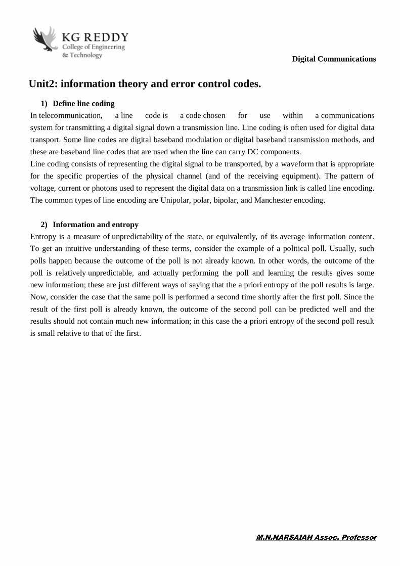
4) Define and explain Huffman code Huffman code is a particular type of optimal prefix code that is commonly used for lossless data compression. The process of finding and/or using such a code proceeds by means of Huffman coding, an algorithm developed by David A. Huffman while he was a Sc.D. student at MIT, and published in the 1952 paper "A Method for the Construction of Minimum-Redundancy Codes". The output from Huffman's algorithm can be viewed as a variable-length code table for encoding a source symbol (such as a character in a file). The algorithm derives this table from the estimated probability or frequency of occurrence (weight) for each possible value of the source symbol. As in other entropy encoding methods, more common symbols are generally represented using fewer bits than less common symbols. Huffman's method can be efficiently implemented, finding a code in time linear to the number of input weights if these weights are sorted. However, although optimal among methods encoding symbols separately, Huffman coding is not always optimal among all compression methods.
a very simple
their frequencies, into a new symbol. We do this repeatedly until we only have one symbol. The result is a
symbols {a,b,c,d,e,o, k} with differing probabilities (Figure 1). The codeword for each symbol is the sequences of left (0) and right (1) moves required to reach that symbol from the top of the tree. Notice that in this example we have 7 symbols, so the naive fixed-length code would require 3 bits per symbol ( 2 8 7 3 = ! ). The Huffman code (which is variable-length) requires on average 2.48 bits; while the entropy gives a lower bound of 2.41 bits. The fact that it is a prefix code makes it easy to decode a string symbol by symbol by starting from the top of the tree and moving down left or right every time a new bit arrives. For example, try decoding: 1010011010010100.
Digital Communications
5) Define and explain Variable length coding In coding theory a variable-length code is a code which maps source symbols to a variable number of bits. Variable-length codes can allow sources to be compressed and decompressed with zero error (lossless data compression) and still be read back symbol by symbol. With the right coding strategy an independent and identically-distributed source may be compressed almost arbitrarily close to its entropy. This is in contrast to fixed length coding methods, for which data compression is only possible for large blocks of data, and any compression beyond the logarithm of the total number of possibilities comes with a finite (though perhaps arbitrarily small) probability of failure. Some examples of well-known variable-length coding strategies are Huffman coding, Lempel Ziv coding and arithmetic coding. Codes and their extensions The extension of a code is the mapping of finite length source sequences to finite length bit strings, that is obtained by concatenating for each symbol of the source sequence the corresponding codeword produced by the original code. Using terms from formal language theory, the precise mathematical definition is as follows: Let {S} and {T} be two finite sets, called the source and target alphabets, respectively. A code {\ C:S\to
T^{*}} is a total function mapping each symbol from {S} to a sequence of symbols over {T},and the
extension of {C} to a homomorphism of {S^{*}} T^{*}}which naturally maps each sequence of source symbols to a sequence of target symbols, is referred to as its extension.

Digital CommunicationsClasses of variable-length codes[edit] Variable-length codes can be strictly nested in order of decreasing generality as non-singular codes, uniquely decodable codes and prefix codes. Prefix codes are always uniquely decodable, and these in turn are always non-singular: Non-singular codes A code is non-singular if each source symbol is mapped to a different non-empty bit string, i.e. the mapping from source symbols to bit strings is injective. For example the mapping is not non-singular because both "a" and "b" map to the same bit string "0" ; any extension of this mapping will generate a lossy (non-lossless) coding. Such singular coding may still be useful when some loss of information is acceptable (for example when such code is used in audio or video compression, where a lossy coding becomes equivalent to source quantization). However, the mapping is non-singular ; its extension will generate a lossless coding, which will be useful for general data transmission (but this feature is not always required). Note that it is not necessary for the non-singular code to be more compact than the source (and in many applications, a larger code is useful, for example as a way to detect and/or recover from encoding or transmission errors, or in security applications to protect a source from undetectable tampering). Uniquely decodable codes A code is uniquely decodable if its extension is non-singular (see above). Whether a given code is uniquely decodable can be decided with the Sardinas Patterson algorithm. The mapping is uniquely decodable (this can be demonstrated by looking at the follow-set after each target bit string in the map, because each bit string is terminated as soon as we see a 0 bit which cannot follow any existing code to create a longer valid code in the map, but unambiguously starts a new code). Consider again the code from the previous section. This code, which is based on an example found in,[1] is not uniquely decodable, since the string 011101110011 can be interpreted as the sequence of
01110 1110 011 1 011 10011. Two possible decoding of this encoded string are thus given by cdb and babe. However, such a code is useful when the set of all possible source symbols is completely known and finite, or when there are restrictions (for example a formal syntax) that determine if source elements of this extension are acceptable. Such restrictions permit the decoding of the original message by checking which of the possible source symbols mapped to the same symbol are valid under those restrictions. Main article: Prefix code A code is a prefix code if no target bit string in the mapping is a prefix of the target bit string of a different source symbol in the same mapping. This means that symbols can be decoded instantaneously after their entire codeword is received. Other commonly used names for this concept are prefix-free code, instantaneous code, or context-free code.

Digital CommunicationsThe example mapping M_{3} in the previous paragraph is not a prefix code because we don't know after reading the bit string "0" if it encodes an "a" source symbol, or if it is the prefix of the encodings of the "b" or "c" symbols. An example of a prefix code is shown below.
Symbol Codeword
a 0
b 10
c 110
d 111
Example of encoding and decoding:
A special case of prefix codes are block codesare not very useful in the context of source coding, but often serve as error correcting codes in the context of channel coding. Another special case of prefix codes are variable-length quantity codes, which encode arbitrarily large integers as a sequence of octets -- i.e., every codeword is a multiple of 8 bits. Advantages The advantage of a variable-length code is that unlikely source symbols can be assigned longer codewords
expected codeword length.

Digital Communications Unit3: Baseband pulse and pass-band transmission
1) Digital subscriber line
Digital subscriber line (DSL; originally digital subscriber loop) is a family of technologies that are used
to transmit digital data over telephone lines. In telecommunications marketing, the term DSL is widely
understood to mean asymmetric digital subscriber line(ADSL), the most commonly installed DSL
technology, for Internet access. DSL service can be delivered simultaneously with wired telephone
service on the same telephone line since DSL uses higher frequency bands for data. On the customer
premises, a DSL filteron each non-DSL outlet blocks any high-frequency interference to enable
simultaneous use of the voice and DSL services.
The bit rate of consumer DSL services typically ranges from 256 kbit/s to over 100 Mbit/s in the direction
to the customer (downstream), depending on DSL technology, line conditions, and service-level
implementation. Bit rates of 1 Gbit/s have been reached in trials,[1] but most homes are likely to be limited
to 500-800 Mbit/s. In ADSL, the data throughput in the upstream direction (the direction to the service
provider) is lower, hence the designation of asymmetric service. In symmetric digital subscriber
line (SDSL) services, the downstream and upstream data rates are equal. Researchers at Bell Labs have
reached speeds of 10 Gbit/s, while delivering 1 Gbit/s symmetrical broadband access services using
traditional copper telephone lines.
2) BASEBAND M-ARY PAM TRANSMISSION
Partial response signalling (PRS), also known as correlative coding, was introduced for the first time in
1960s for high data rate communication [lender, 1960]. From a practical point of view, the background of
this technique is related to the Nyquist criterion.
Assume a Pulse Amplitude Modulation (PAM), according to the Nyquist criterion, the highest possible
transmission rate without Inter-symbol-interference (ISI) at the receiver over a channel with a bandwidth of
W (Hz) is 2W symbols/sec.
3) BASEBAND M-ARY PAM TRANSMISSION
Up to now for binary systems the pulses have two possible amplitude levels. In a baseband M-ary PAM
system, the pulse amplitude modulator produces M possible amplitude levels with M>2. In an M-ary
system, the information source emits a sequence of symbols from an alphabet that consists of M symbols.
Each amplitude level at the PAM modulator output corresponds to a distinct symbol. The symbol duration
T is also called as the signaling rate of the system, which is expressed as symbols per second or bauds.

Digital Communications
consists of two bits.
The symbol duration T of the M-ary system is related to the bit duration Tb of the equivalent binary PAM
system as For a given channel bandwidth, using M-ary PAM system, log2M times more information is
transmitted than binary PAM system. T = Tb log2 M transmitted than binary PAM system. The price we
paid is the increased bit error rate compared binary PAM system. To achieve the same probability of error
as the binary PAM system, the transmit power in <-ary PAM system must be increased.
For M much larger than 2 and an average probability of symbol error small compared to 1, the transmitted
power must be increased by a factor of M2/log2M compared to binary PAM system. The M-ary PAM
transmitter and receiver is similar to the binary PAM transmitter and receiver. In transmitter, the M-ary
pulse train is shaped by a transmit filter and transmitted through a channel which corrupts the signal with
noise and ISI. The received signal is passed through a receive filter and sampled at an appropriate rate in
synchronism with the transmitter. Each sample is compared with preset threshold values and a decision is
made as to which symbol was transmitted. Obviously, in M-ary system there is an M-1 threshold level
which makes the system complicated.
4) Explain Adaptive equalization
An adaptive equalizer is an equalizer that automatically adapts to time-varying properties of
the communication channel. It is frequently used with coherent modulations such as phase shift keying,
mitigating the effects of multipath propagation and Doppler spreading.
Many adaptation strategies exist. They include:
Note that the receiver does not have access to the transmitted signal x when it is not in
training mode. If the probability that the equalizer makes a mistake is sufficiently small, the symbol
decisions d(n) made by the equalizer may be substituted for x
A well-known example is the , a filter that uses feedback of detected in
addition to conventional equalization of future symbols. Some systems use predefined training sequences
to provide reference points for the adaptation process.
5) Explain Matched filter
In signal processing, a matched filter is obtained by correlating a known signal, or template, with an
unknown signal to detect the presence of the template in the unknown signal.[1][2] This is equivalent to
convolving the unknown signal with a conjugated time-reversed version of the template. The matched filter
is the optimal linear filter for maximizing the signal to noise ratio (SNR) in the presence of additive
stochastic noise. Matched filters are commonly used in radar, in which a known signal is sent out, and the

Digital Communicationsreflected signal is examined for common elements of the out-going signal. Pulse compression is an
example of matched filtering. It is so called because impulse response is matched to input pulse signals.
Two-dimensional matched filters are commonly used in image processing, e.g., to improve SNR for X-ray.
Matched filtering is a demodulation technique with LTI (linear time invariant) filters to maximize SNR.[3]
It was originally also known as a North filter.
MATCHED FILTER
Since each of t
the interval 0<t<T. we can design a linear filter with impulse response hj(t), with the received signal x(t)
the fitter output is given by the convolution integral
where xj is the j th correlator output produced by the received signal x(t).
A filter whose impulse response is time-reversed and delayed version of the input signal is said to be
matched. Correspondingly , the optimum receiver based on this is referred as the matched filter receiver.
For a matched filter operating in real time to be physically realizable, it must be causal. For causal system

Digital Communications
h(t) = impulse response W(t) =white noise
The impulse response of the matched filter is time-reversed and delayed version of the input signal.

Digital Communications
Unit4: digital modulation techniques. 1) Explain Coherent and non coherent ASK detector
Amplitude-shift keying (ASK) is a form of amplitude modulation that represents digital data as
variations in the amplitude of a carrier wave. In an ASK system, the binary symbol 1 is represented by
transmitting a fixed-amplitude carrier wave and fixed frequency for a bit duration of T seconds. If the
signal value is 1 then the carrier signal will be transmitted; otherwise, a signal value of 0 will be
transmitted.
Any digital modulation scheme uses a finite number of distinct signals to represent digital data. ASK uses
a finite number of amplitudes, each assigned a unique pattern of binary digits. Usually, each amplitude
encodes an equal number of bits. Each pattern of bits forms the symbol that is represented by the
particular amplitude. The demodulator, which is designed specifically for the symbol-set used by the
modulator, determines the amplitude of the received signal and maps it back to the symbol it represents,
thus recovering the original data. Frequency and phase of the carrier are kept constant.
In transmitter the binary data sequence is given to an on- ff enc der. This gives an output Eb volts
for symbol 1 and 0 volt for symbol 0. The resulting binary wave [in Unipolar form] and sinusoidal carrier
1 (t) are applied to a product modulator. The desired BASK wave is obtained at the modulator output.
In demodulator, the received noisy BASK signal x(t) is apply to correlator with coherent reference signal
1 (t) as shown in fig. (b). he correlator output x is compared with

Digital Communications
2) Define QPSK.
In QPSK two successive bits in the data sequence are grouped together. This combination of two bits
forms four distinct symbols. When the symbol is changed to next symbol the phase of the carrier is
Because of combination of two bits there will be four symbols. Hence
QPSK reduces amplitude variations and required transmission bandwidth.
3) Explain ASK Modulator
Amplitude-shift keying (ASK) is a form of amplitude modulation that represents digital data as variations
in the amplitude of a carrier wave. In an ASK system, the binary symbol 1 is represented by transmitting a
fixed-amplitude carrier wave and fixed frequency for a bit duration of T seconds. If the signal value is 1
then the carrier signal will be transmitted; otherwise, a signal value of 0 will be transmitted.
Any digital modulation scheme uses a finite number of distinct signals to represent digital data. ASK uses
a finite number of amplitudes, each assigned a unique pattern of binary digits. Usually, each amplitude
encodes an equal number of bits. Each pattern of bits forms the symbol that is represented by the
particular amplitude. The demodulator, which is designed specifically for the symbol-set used by the
modulator, determines the amplitude of the received signal and maps it back to the symbol it represents,
thus recovering the original data. Frequency and phase of the carrier are kept constant.
4) Define FSK

Digital CommunicationsFrequency-shift keying (FSK) is a frequency modulation scheme in which digital information is
transmitted through discrete frequency changes of a carrier signal.[1] The technology is used for
communication systems such as amateur radio, caller ID and emergency broadcasts. The simplest FSK
is binary FSK (BFSK). BFSK uses a pair of discrete frequencies to transmit binary (0s and 1s)
information.[2] With this scheme, the "1" is called the mark frequency and the "0" is called the space
frequency.
5) Explain Frequency spectrum of FSK

Digital Communications

Digital Communications
Unit5: Spread Spectrum Modulation 1) Applications of SSM
The SS Communications are widely used today for Military, Industrial, Avionics, Scientific, and Civil uses. The applications include the following:
1. Jam-resistant communication systems 2. CDMA radios: It is useful in multiple access communications wherein many users communicate
over a shared channel. Here the assignment of a unique spread spectrum sequence to each user allows him to simultaneously transmit over a common channel with minimal mutual interference. Such access technique often simplifies the network control requirements considerably.
3. High Resolution Ranging: SS Communications is often used in high resolution ranging. It is possible to locate an object with good accuracy using SS techniques. One example where it could be used is Global Positioning System (GPS). Here an object can use signals from several satellites transmitting SS signals according to a predefined format to determine its own position accurately on the globe.
4. WLAN: Wireless LAN (Local Area Networks) widely use spread spectrum communications. IEEE 802.11 is a standard that is developed for mobile communication, and widely implemented throughout the world. The standard defines three types of Physical Layer communications. These are:
a. Infrared (IR) Communications b. Direct Sequence Spread Spectrum Communications c. Frequency Hopping Spread Spectrum Communications.
Among the three, DSSS, and FHSS are widely used.
5. Cordless Phones: Several manufacturers implement Spread Spectrum in Cordless phones. The advantages of using spread spectrum in cordless phone include the following:
a. Security: Inherently, a ss communication is coded. b. Immunity to Noise: SS modulation is immune to noise when compared with other
modulation schemes such as AM and FM. c. Longer Range: Due to noise immunity, it is possible to achieve a longer range of
communications, for a very small transmitted power. 6. Long-range wireless phones for home and industry 7. Cellular base stations interconnection.
2) Frequency hoping spread spectrum (FHSS)

Digital CommunicationsHere the transmitted signal appears as a data modulated carrier which is hopping from one frequency to next, and therefore, it is called frequency hopping spread spectrum (FH-SS). FH systems work by driving a frequency synthesizer with pseudorandom sequence of numbers that result in the synthesizer hopping different frequencies at different points, and thus achieving signal spread. At the receiver end, the same principle works. A synthesizer is driven by a matching code to achieve maximum threshold detection of received signals. A simplified block schematic of a FH SS system is shown below: 1. FH-SS Transmitter: The transmitter consists of a baseband modulator followed by frequency synthesizer. The frequency synthesizer is driven by a PN generator. A PN generator may be built internal to the synthesizer.
2. FH-SS Receiver: A FH-SS receiver consists of a down converter followed by a demodulator. A synthesizer, driven by a matching PN generator is used to down convert the received signals. A maximum received signal threshold signifies locking.
c. Time Hopping (TH) SS Systems:
Time hopping is not used as frequency as DSSS and FHSS. Time Hopping to spread the carrier is achieved by randomly spacing narrow transmitted pulses. The multiplicity factor is given by: Multiplicity factor = (average pulse spacing) / (pulse width). d. Recovery of Spread Spectrum Signals: Important Timing Signals In all cases of SS receivers, faithful recovery of the transmitted signals requires the following:
Digital Communicationsa. Correlation Interval Synchronization: Receiving bits is achieved by proper correlator (or integrator) timing. Proper start/stop times for correlator are required for minimizing the received bit errors. b. SS Generator Synchronization: Timing signals are required to control the SS wave form generator signals. Direct Sequence systems employ a clock ticking at the chip rate 1/tc, and FH systems have a clock operating at the hopping rate. c. Carrier Synchronization: Faithful reproduction of the transmitted signals to baseband requires down-conversion, and demodulation. This can be achieved only if the locally generated frequency and phase are in sync with the received carrier frequency.
3. Comparison of DSSS & FHSS
FHSS vs DSSS
Spread spectrum is a group of techniques that utilizes a much larger bandwidth in transmitting information than would otherwise occupy a fraction of the bandwidth used. This is done to achieve a certain effect. FHSS and DSSS, which stand for Frequency Hopping Spread Spectrum and Direct Sequence Spread Spectrum, are two spread spectrum techniques. The main difference is in how they spread the data into the wider bandwidth. FHSS utilizes frequency hopping while DSSS utilizes pseudo noise to modify the phase of the signal.
Frequency hopping is achieved by dividing the large bandwidth into smaller channels that would fit the data. The signal would then be sent pseudo-randomly into a different channel. Because only one of the channels is in use at any given time, you are actually wasting bandwidth equivalent to the data bandwidth multiplied by the number of channels minus one. DSSS spreads the information across the band in a very different manner. It does so by introducing pseudo-random noise into the signal to change its phase at any given time. This results in an output that closely resembles static noise and would appear as just that to
- om the noise as long as the pseudo-random sequence is known.
In order for the receiver to decode the transmitted information, it must be synchronized with the transmitter. For FHSS it is relatively easy as the transmitter simply waits on one of the channels and waits for a decodable transmission. Once it finds that out, it can then follow the sequence being used to follow the transmitter which jumps across the different channels. With DSSS, it is not as simple. A timing search algorithm needs to be employed for the receiver to correctly establish synchronization.

Digital Communications
4) Define Pseudo noise (PN) sequence
In cryptography, pseudorandom noise (PRN) is a signal similar to noise which satisfies one or more of the standard tests for statistical randomness. Although it seems to lack any definite pattern, pseudorandom noise consists of a deterministic sequence of pulses that will repeat itself after its period. In cryptographic devices, the pseudorandom noise pattern is determined by a key and the repetition period can be very long, even millions of digits. Pseudorandom noise is used in some electronic musical instruments, either by itself or as an input to subtractive synthesis, and in many white noise machines. In spread-spectrum systems, the receiver correlates a locally generated signal with the received signal. Such spread-spectrum systems require a set of one or more "codes" or "sequences" such that
Like random noise, the local sequence has a very low correlation with any other sequence in the set, or with the same sequence at a significantly different time offset, or with narrow band interference, or with thermal noise.
Unlike random noise, it must be easy to generate exactly the same sequence at both the transmitter and the receiver, so the receiver's locally generated sequence has a very high correlation with the transmitted sequence.

Digital Communications5) What is Code Division Multiple Access (CDMA) CDMA employs analog-to-digital conversion (ADC) in combination with spectrum technology. Audio input is first digitized into binary elements. The frequency of the transmitted signal is then made to vary according to a defined pattern (code), so it can be intercepted only by a receiver whose frequency response is programmed with the same code, so it follows exactly along with the transmitter frequency. There are trillions of possible frequency-sequencing codes, which enhance privacy and makes cloning difficult.

Digital Communications 15) TUTORIAL TOPICS
UNIT I:
1) Advantages of Digital communication over Analog communication 2) Elements of Digital Communication 3) Sampling theorem 4) Errors in Delta modulation
UNIT II:
1) Entropy 2) Shannon fano coding 3) Huffman coding 4) Linear block codes 5) Cyclic code 6) Convolution codes
UNIT III:
1) Matched Filter Receiver 2) Probability of errors 3) Eye pattern
UNIT IV:
1) Digital modulation techniques like ASK, PSK, FSK 2) Quadrature phase shift keying (QPSK) 3) Binary phase shift keying (BPSK)
UNIT V:
1) Direct sequence spread spectrum (DSSS) 2) Frequency hopping spread spectrum (FHSS) 3) Generation and character tics of PN sequence
Digital Communications16) Unit Wise Question Bank:
Unit1 1. Two marks questions with answer
1) What is communication (or Telecommunication) Ans- The term communication (or telecommunication) means the transfer of some form of information from one place (known as the source of information) to another place (known as the destination of information) using some system to do this function (known as a communication system)
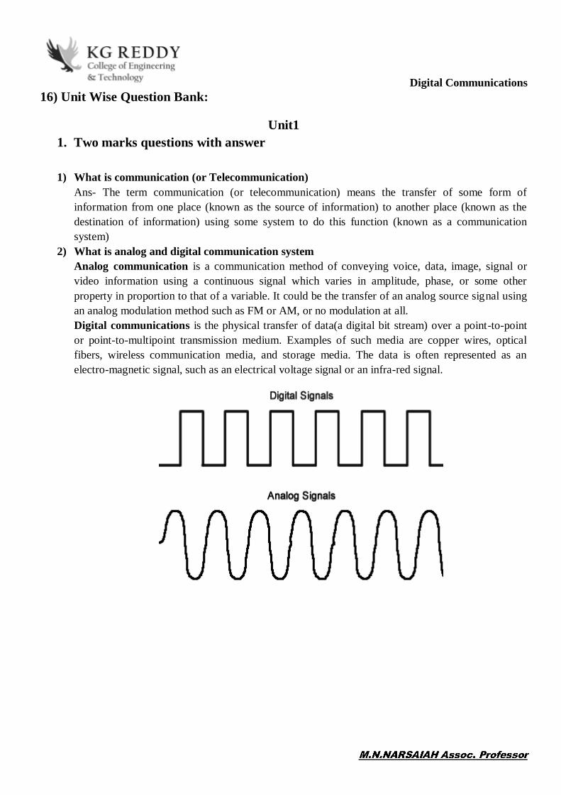
2) What is analog and digital communication system Analog communication is a communication method of conveying voice, data, image, signal or video information using a continuous signal which varies in amplitude, phase, or some other property in proportion to that of a variable. It could be the transfer of an analog source signal using an analog modulation method such as FM or AM, or no modulation at all. Digital communications is the physical transfer of data(a digital bit stream) over a point-to-point or point-to-multipoint transmission medium. Examples of such media are copper wires, optical fibers, wireless communication media, and storage media. The data is often represented as an electro-magnetic signal, such as an electrical voltage signal or an infra-red signal.

Digital Communications
3) What is Quantization Noise
process introduces an error defined as the difference between the input signal, x (t) and the output signal, y ( q(t) = x(t) y(t) Quantization noise is produced in the transmitter end of a PCM system by rounding off sample values of an analog base-band signal to the nearest permissible representation levels of the quantizer. As such quantization noise differs from channel noise in that it is signal dependent.
4) What is Companding
In telecommunication companding (occasionally called compansion) is a method of mitigating the detrimental effects of a channel with limited dynamic range. The name is a portmanteau of the words compressing and expanding. The use of companding allows signals with a large dynamic range to be transmitted over facilities that have a smaller dynamic range capability. Companding is employed in telephony and other audio applications such as professional wireless microphones and analog recording.

Digital Communications
5) Define noises in PCM &DM The two sources of noise in delta modulation are "slope overload", when step size is too small to track the original waveform, and "granularity", when step size is too large.
2. THREE MARKS QUESTIONS WITH ANSWER
Advantages of digital communication system Ans - The digital communication has mostly common structure of encoding a signal so devices
used are mostly similar. The Digital Communication's main advantage is that it provides us added security to our
information signal. The digital Communication system has more immunity to noise and external interference. Digital information can be saved and retrieved when necessary while it is not possible in analog. Digital Communication is cheaper than Analog Communication.
Digital Communications The configuring process of digital communication system is simple as compared to analog
communication system. Although, they are complex. In Digital Communication System, the error correction and detection techniques can be
implemented easily.
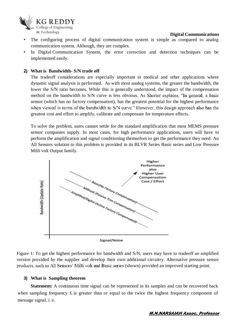
What is Bandwidth- S/N trade off The tradeoff considerations are especially important in medical and other applications where dynamic signal analysis is performed. As with most analog systems, the greater the bandwidth, the lower the S/N ratio becomes. While this is generally understood, the impact of the compensation method on the bandwidth to S/N curve is less obvious. As sensor (which has no factory compensation), has the greatest potential for the highest performance
greatest cost and effort to amplify, calibrate and compensate for temperature effects. To solve the problem, users cannot settle for the standard amplification that most MEMS pressure sensor companies supply. In most cases, for high performance applications, users will have to perform the amplification and signal conditioning themselves to get the performance they need. An All Sensors solution to this problem is provided in its BLVR Series Basic series and Low Pressure Milli volt Output family.
Figure 1: To get the highest performance for bandwidth and S/N, users may have to tradeoff an amplified version provided by the supplier and develop their own additional circuitry. Alternative pressure sensor
(shown) provided an improved starting point.
What is Sampling theorem
Statement: A continuous time signal can be represented in its samples and can be recovered back when sampling frequency fs is greater than or equal to the twice the highest frequency component of message signal. i. e.

Digital Communications
Proof: Consider a continuous time signal x(t). The spectrum of x(t) is a band limited to fm Hz i.e. the m.
s. The output of multiplier is a discrete signal called sampled signal which is represented with y(t) in the following diagrams:
Here, you can observe that the sampled signal takes the period of impulse. The process of sampling can be explained by the following mathematical expression:
What is Hartley shanon law
the Shannon Hartley theorem tells the maximum rate at which information can be transmitted over a communications channel of a specified bandwidth in the presence of noise. It is an application of the noisy-channel coding theorem to the archetypal case of a continuous-time analog communications channel subject to Gaussian noise. The theorem establishes Shannon's channel capacity for such a communication link, a bound on the maximum amount of error-free information per time unit that can be transmitted with a specified bandwidth in the presence of the noise interference, assuming that the signal power is bounded, and that the Gaussian noise process is characterized by a known power or power spectral density. The law is named after Claude Shannon and Ralph Hartley. Formulated as
Where C is the channel capacity in bits per second, a theoretical upper bound on the net bit rate (information rate, sometimes denoted I) excluding error-correction codes; B is the bandwidth of the channel in hertz (pass band bandwidth in case of a band pass signal);
Digital CommunicationsS is the average received signal power over the bandwidth (in case of a carrier-modulated pass band transmission, often denoted C), measured in watts (or volts squared); N is the average power of the noise and interference over the bandwidth, measured in watts (or volts squared); and S/N is the signal-to-noise ratio (SNR) or the carrier-to-noise ratio (CNR) of the communication signal to the noise and interference at the receiver (expressed as a linear power ratio, not as logarithmic decibels).
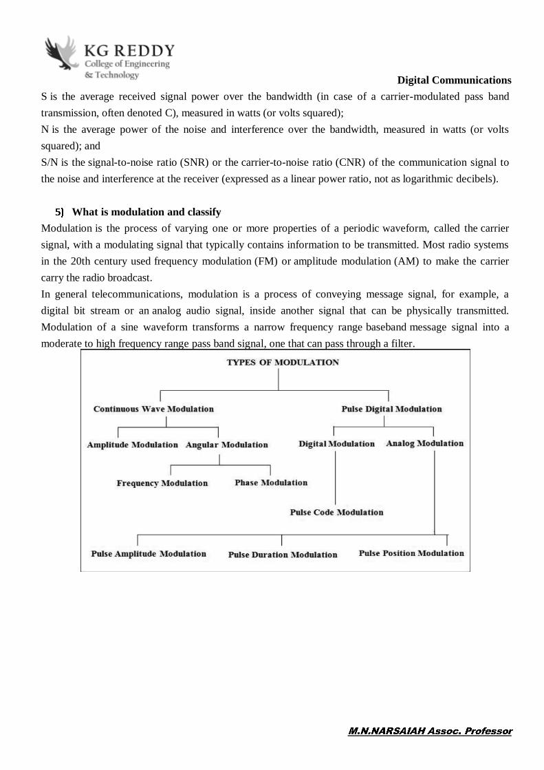
What is modulation and classify Modulation is the process of varying one or more properties of a periodic waveform, called the carrier signal, with a modulating signal that typically contains information to be transmitted. Most radio systems in the 20th century used frequency modulation (FM) or amplitude modulation (AM) to make the carrier carry the radio broadcast. In general telecommunications, modulation is a process of conveying message signal, for example, a digital bit stream or an analog audio signal, inside another signal that can be physically transmitted. Modulation of a sine waveform transforms a narrow frequency range baseband message signal into a moderate to high frequency range pass band signal, one that can pass through a filter.

Digital Communications3. FIVE MARKS QUESTIONS WITH ANSWER
1) Write a note on PCM generation and reconstruction
Pulse-code modulation or PCM is known as a digital pulse modulation technique. In fact, the pulse-code modulation is quite complex as compared to the analog pulse modulation techniques i.e. PAM, PWM and PPM, in the sense that the message signal is subjected to a great number of operations. Fig.1 shows the basic elements of a PCM system .
c) : Receiver Fig.1 : The basic elements of a PCM System It consists of three main parts i.e. , Transmitter Transmission path Receiver The essential operation in the transmitter of a PCM system are : Sampling Quantizing Encoding This is shown in fig.2.

Digital CommunicationsThe human voice uses frequencies between 100Hz and 10,000Hz, but it has been found that most of the energy in speech is between 300 Hertz and 3400 Hertz - a bandwidth of approximately 3100 Hertz. Before converting the signal from analog to digital, the unwanted frequency components of the signal are filtered out. This makes the task of converting the signal to digital form much easier, and results in an acceptable quality of signal reproduction for voice communication. From an equipment point of viev, because the manufacture of very precise filters would be expensive, a bandwidth of 4000 Hertz is generally used. This bandwidth limitation also helps to reduce aliasing - aliasing happens when the number of samples is insufficient to adequately represent the analog waveform (the same effect you can see on a computer screen when diagonal and curved lines are displayed as a series of zigzag horizontal and vertical lines).
Sampling is the process of reading the values of the filtered analogue signal at discrete time intervals (i.e. at a constant sampling rate, called the sampling frequency). A scientist called Harry Nyquist discovered that the original analogue signal could be reconstructed if enough samples were taken. He found that if the sampling frequency is at least twice the highest frequency of the input analogue signal, the signal could be reconstructed using a low-pass filter at the destination.
Quantization is the process of assigning a discrete value from a range of possible values to each sample obtained. The number of possible values will depend on the number of bits used to represent each sample. Quantization can be achieved by either rounding the signal up or down to the nears available value, or truncating the signal to the nearest value which is lower than the actual sample. The process results in a stepped waveform resembling the source signal. The difference between the sample and the value assigned to it is known as the quantization noise (or quantization error).
Quantization noise can be reduced by increasing the number of quantization intervals, because the difference between the input signal amplitude and the quantization interval decreases as the number of quantization intervals increases. This would, however, increase the PCM bandwidth. Uniform quantization uses equal quantization levels throughout the entire range of an input analogue signal. The signal-to-noise ratio (SNR), including quantization noise, is the most important factor affecting voice quality in uniform quantization. The signal-to-noise ratio is measured in decibels (dB). The higher the signal-to-noise ratio, the better the voice quality. Quantization noise reduces the signal-to-noise ratio of a signal, so an increase in quantization noise degrades the quality of a voice signal. Low signals will have a small signal-to-noise ratio and high signals will have a large signal-to-noise ratio. Because most voice signals are relatively low, having better voice quality at higher signal levels is an inefficient way of digitizing voice signals. Uniform quantization was therefore replaced by a non-uniform quantization process called companding (see below). Narrowband speech is typically sampled 8000 times per second, and each sample must be quantized. If linear quantization is used, 12 bits per sample are required, giving a bit rate of 96 Kbits per second. This

Digital Communicationscan be reduced using non-linear quantization, in which 8 bits per sample is sufficient to provide speech quality almost indistinguishable from the original. This results in a bit rate of 64 Kbits per second. Two non-linear PCM were standardized in the 1960s - µ-law (mu-law) coding was the standard developed in the United States, while A-law compression was used in Europe. These are still widely used today. Encoding is the process of representing the sampled values as a binary number in the range 0 to n. The value of n is chosen as a power of 2, depending on the accuracy required. Increasing n reduces the step size between adjacent quantization levels and hence reduces the quantization noise. The down side of this is that the amount of digital data required representing the analogue signal increases.
Stages in the analogue-to-digital conversion process
Companding
Working with very small signal levels (by comparison with the quantization interval) can introduce more errors. Companding can be used to increase the accuracy of such signals. This is the process of distorting the analogue signal in a controlled way before quantizing takes place, by compressing its larger values at the source and then expanding them at the receiving end. There are two standards used: A-law in Europe, and µ-law in the USA. The term Companding was created by combining the terms compressing and expanding. Input analog signal samples are compressed into logarithmic segments. Each segment is then quantized, and coded using uniform quantization. The compression process is logarithmic, where the compression increases as the sample signals increase (the larger sample signals are compressed more than the smaller sample signals, causing the quantization noise to increase as the sample signal increases). A logarithmic increase in quantization noise throughout the dynamic range of an input sample signal gives a signal-to-noise ratio which is almost constant over a wide range of input levels. A rate of eight bits per sample (64 Kbits per second) gives a reconstructed signal which is very close the original. The advantages of this system include low complexity and delay, and high-quality reproduction of speech. The disadvantages are a relatively high bit rate and a high susceptibility to channel errors.

Digital CommunicationsSimilarities between A-law and µ-law:
6) Both are linear approximations of a logarithmic input/output relationship
7) Both are implemented using 8-bit code words (256 levels, one for each quantization interval).
This allows for a bit rate of 64 Kbits per second
8) Both break the dynamic range into 16 segments (8 positive and 8 negative) - each segment is
twice the length of the preceding one, and uniform quantization is used within each segment
9) Both use similar encoding techniques for the 8-bit word - the first (most significant bit)
identifies polarity, bits 2, 3 and 4 identify the segment, and the last four bits identify the
quantization level within the segment
Differences between A-law and µ-law:
10) Different linear approximations lead to different lengths and slopes
11) Numerical assignment of the bit positions in the 8-bit code word to segments and to
quantization levels within segments are different
12) A-law provides a greater dynamic range
13) µ-law provides better signal/distortion performance for low level signals
14) A-law requires 13 bits for a uniform PCM equivalent, whereas m-law requires 14 bits
15) International connections should use A-law (µ to A conversion is the responsibility of the µ-
law country)
2) Explain Differential pulse code modulation (DPCM)
Differential pulse code modulation (DPCM) is a procedure of converting an analog into a digital signal in which an analog signal is sampled and then the difference between the actual sample value and its predicted value (predicted value is based on previous sample or samples) is quantized and then encoded forming a digital value. DPCM code words represent differences between samples unlike PCM where code words represented a sample value. Basic concept of DPCM - coding a difference, is based on the fact that most source signals show significant correlation between successive samples so encoding uses redundancy in sample values which implies lower bit rate. Realization of basic concept (described above) is based on a technique in which we have to predict current sample value based upon previous samples (or sample) and we have to encode the difference between actual value of sample and predicted value (the difference between samples can be interpreted as prediction error).Because it's necessary to predict sample value DPCM is form of predictive coding.

Digital CommunicationsDPCM compression depends on the prediction technique, well-conducted prediction techniques lead to good compression rates, in other cases DPCM could mean expansion comparing to regular PCM encoding.
Fig 1. DPCM encoder (transmitter)
3) Write a note on Adaptive differential pulse-code modulation (ADPCM)
Adaptive differential pulse-code modulation (ADPCM) is a variant of differential pulse-code modulation (DPCM) that varies the size of the quantization step, to allow further reduction of the required data bandwidth for a given signal-to-noise ratio. Typically, the adaptation to signal statistics in ADPCM consists simply of an adaptive scale factor before quantizing the difference in the DPCM encoder.
In telephony, a standard audio signal for a single phone call is encoded as 8000 analog samples per second, of 8 bits each, giving a 64 Kbit/s digital signal known as DS0. The default signal compression encoding on a DS0 is either -law (mu-law) PCM (North America and Japan) or A-law PCM (Europe and most of the rest of the world). These are logarithmic compression systems where a 13 or 14 bit linear PCM sample number is mapped into an 8 bit value. This system is described by international standard G.711. Where circuit costs are high and loss of voice quality is acceptable, it sometimes makes sense to compress the voice signal even further. An ADPCM algorithm is used to map a series of 8 bit µ-law (or a-law) PCM samples into a series of 4 bit ADPCM samples. In this way, the capacity of the line is doubled. The technique is detailed in the G.726 standard. Some ADPCM techniques are used in Voice over IP communications. ADPCM was also used by Interactive Multimedia Association for development of legacy audio codec known as ADPCM DVI, IMA ADPCM or DVI4, in the early 1990s.[3] Split-band or sub band ADPCM G.722[4] is an ITU-T standard wideband speech codec operating at 48, 56 and 64 kbit/s, based on sub band coding with two channels and ADPCM coding of each.[5] Before the digitization process, it catches the analog signal and divides it in frequency bands with QMF filters (quadrature mirror filters) to get two sub bands of the signal. When the ADPCM bit stream of each sub band is obtained, the results are

Digital Communicationsmultiplexed and the next step is storage or transmission of the data. The decoder has to perform the reverse process, that is, demultiplex and decode each sub band of the bit stream and recombine them.
Referring to the coding process, in some applications as voice coding, the sub band that includes the voice is coded with more bits than the others. It is a way to reduce the file size.
4) Define and explain Delta modulation
A delta modulation -modulation) is an analog-to-digital and digital-to-analog signal conversion technique used for transmission of voice information where quality is not of primary importance. DM is the simplest form of differential pulse-code modulation (DPCM) where the difference between successive samples is encoded into n-bit data streams. In delta modulation, the transmitted data are reduced to a 1-bit data stream. Its main features are: The analog signal is approximated with a series of segments. Each segment of the approximated signal is compared of successive bits is determined by this comparison. Only the change of information is sent, that is, only an increase or decrease of the signal amplitude from the previous sample is sent whereas a no-change condition causes the modulated signal to remain at the same 0 or 1 state of the previous sample. To achieve high signal-to-noise ratio, delta modulation must use oversampling techniques, that is, the analog signal is sampled at a rate several times higher than the Nyquist rate. Derived forms of delta modulation are continuously variable slope delta modulation, delta-sigma modulation, and differential modulation. Differential pulse-code modulation is the superset of DM. Rather than quantizing the absolute value of the input analog waveform, delta modulation quantizes the difference between the current and the previous step, as shown in the block diagram in Fig. 1.
Fig. 1 Block diagram of a -modulator/demodulator The modulator is made by a Quantizer which converts the difference between the input signal and the average of the previous steps. In its simplest form, the Quantizer can be realized with a comparator referenced to 0 (two levels Quantizer), whose output is 1 or 0 if the input signals is positive or negative. It

Digital Communicationsis also a bit-Quantizer as it quantizes only a bit at a time. The demodulator is simply an integrator (like the one in the feedback loop) whose output rises or falls with each 1 or 0 received. The integrator itself constitutes a low-pass filter.
5) Define and explain Adaptive DM
Adaptive delta modulation (ADM) was first published by Dr. John E. Abate (AT&T Bell Laboratories Fellow) in his doctoral thesis at NJ Institute Of Technology in 1968. ADM was later selected as the standard for all NASA communications between mission control and space-craft. Adaptive delta modulation or [continuously (CVSD) is a modification of DM in which the step size is not fixed. Rather, when several consecutive bits have the same direction value, the encoder and decoder assume that slope overload is occurring, and the step size becomes progressively larger. Otherwise, the step size becomes gradually smaller over time. ADM reduces slope error, at the expense of increasing quantizing error. This error can be reduced by using a low-pass filter. ADM provides robust performance in the presence of bit errors meaning error detection and correction are not typically used in an ADM radio design, it is very useful technique this allows fortive-delta-modulation The performance of a delta modulator can be improved significantly by making the step size of the modulator assume a time-varying form. In particular, during a steep segment of the input signal the step size is increased. Conversely, when the input signal is varying slowly, the step size is reduced. In this way, the size is adapted to the level of the input signal. The resulting method is called adaptive delta modulation (ADM). There are several types of ADM, depending on the type of scheme used for adjusting the step size. In this ADM, a discrete set of values is provided for the step size. Fig.3.17 shows the block diagram of the transmitter and receiver of an ADM System. In practical implementations of the system, the step size

Digital Communications

Digital Communications
4. OBJECTIVE QUESTIONS WITH ANSWERS
1) The modulation techniques used to convert analog signal into digital signal are a) Pulse code modulation b) Delta modulation c) Adaptive delta modulation d) All of the above
ANSWER: d) All of the above 2) The sequence of operations in which PCM is done is a) Sampling, quantizing, encoding b) Quantizing, encoding, sampling c) Quantizing, sampling, encoding d) None of the above ANSWER: a) Sampling, quantizing, encoding 3) In PCM, the parameter varied in accordance with the amplitude of the modulating signal is a) Amplitude b) Frequency c) Phase d) None of the above
ANSWER: d) None of the above

Digital Communications 4) One of the disadvantages of PCM is a) It requires large bandwidth b) Very high noise c) Cannot be decoded easily d) All of the above ANSWER: a) It requires large bandwidth 5) The expression for bandwidth BW of a PCM system, where v is the number of bits per sample and fm is the modulating frequency, is given by a) BW> = vfm b) BW< = vfm c) BW> = 2 vfm d) BW> = 1/2vfm ANSWER: a) BW> = vfm Q6. The error probability of a PCM is a) Calculated using noise and inter symbol interference b) Gaussian noise + error component due to inter symbol interference c) Calculated using power spectral density d) All of the above
ANSWER: d) All of the above Q7. In Delta modulation, a) One bit per sample is transmitted b) All the coded bits used for sampling are transmitted c) The step size is fixed d) Both a) and c) are correct
ANSWER: d) Both a) and c) are correct Q8. In digital transmission, the modulation technique that requires minimum bandwidth is a) Delta modulation b) PCM

Digital Communicationsc) DPCM d) PAM
ANSWER: a) Delta modulation Q9. In Delta Modulation, the bit rate is a) N times the sampling frequency b) N times the modulating frequency c) N times the nyquist criteria d) None of the above ANSWER: a) N times the sampling frequency Q10) In Differential Pulse Code Modulation techniques, the decoding is performed by a) Accumulator b) Sampler c) PLL d) Quantizer
ANSWER: a) Accumulator
Digital Communications
5. FILL IN THE BLANK QUESTIONS WITH ANSWERS
Unit1: 1) ------------ transmission occupies lower part of the frequency spectrum. 2) In digital communication system, the information signal is a ------------ message. 3) ----------- is a process of approximation or rounding off. 4) Communication can be kept ------ and -------- 5) Source coding is that it reduces the ----------- requirement. 6) In digital communication, --------- is used for multiplexing. 7) ---------- is non uniform quantization. 8) In ----------- difference between present sample value and previous sample value is transmitted. 9) -------- modulation transmits only one bit per sample instead of N bits transmitted in PCM. 10) --------- & ----------- noise present in Delta modulation.
Ans: 1) Baseband 2) Discrete 3) Quantization 4) Private and secure 5) Bandwidth 6) TDM 7) Companding 8) DPCM 9) Delta 10) Slope overload error and granular

Digital CommunicationsUnit 2
1. TWO MARKS QUESTION WITH ANSWERS 1) Define line coding
In telecommunication, a line code is a code chosen for use within a communications system for transmitting a digital signal down a transmission line. Line coding is often used for digital data transport. Some line codes are digital baseband modulation or digital baseband transmission methods, and these are baseband line codes that are used when the line can carry DC components. Line coding consists of representing the digital signal to be transported, by a waveform that is appropriate for the specific properties of the physical channel (and of the receiving equipment). The pattern of voltage, current or photons used to represent the digital data on a transmission link is called line encoding. The common types of line encoding are Unipolar, polar, bipolar, and Manchester encoding.
2) Give classification of line coding
3) Properties of line coding Transmission Bandwidth: as small as possible Power Efficiency: As small as possible for given BW and probability of error Error Detection and Correction capability: Ex: Bipolar Favorable power spectral density: dc=0 Adequate timing content: Extract timing from pulses Transparency: Prevent long strings of 0s or 1s

Digital Communications4) Define cyclic code
In coding theory, a cyclic code is a block code, where the circular shifts of each codeword gives another word that belongs to the code. They are error-correcting codes that have algebraic properties that are convenient for efficient error detection and correction.
Let{C} be a linear code over a finite field (also called Galois field) {GF(q)} of block length n. {C} is called a cyclic code if, for every codeword c=(c1,...,cn) from C, the word (cn,c1,...,cn-1) in {GF(q)^{n}} obtained by a cyclic right shift of components is again a codeword. Because one cyclic right shift is equal to n 1 cyclic left shifts, a cyclic code may also be defined via cyclic left shifts. Therefore the linear code {C} is cyclic precisely when it is invariant under all cyclic shifts. Cyclic Codes have some additional structural constraint on the codes. They are based on Galois fields and because of their structural properties they are very useful for error controls. Their structure is strongly related to Galois fields because of which the encoding and decoding algorithms for cyclic codes are computationally efficient.
5) Define convolution code In telecommunication, a convolution code is a type of error-correcting code that generates parity symbols via the sliding application of a Boolean polynomial function to a data stream. The sliding application represents the 'convolution' of the encoder over the data, which gives rise to the term 'convolution coding.' The sliding nature of the convolution codes facilitates trellis decoding using a time-invariant trellis. Time invariant trellis decoding allows convolution codes to be maximum-likelihood soft-decision decoded with reasonable complexity. The ability to perform economical maximum likelihood soft decision decoding is one of the major benefits of convolution codes. This is in contrast to classic block codes, which are generally represented by a time-variant trellis and therefore are typically hard-decision decoded. Convolution codes are often characterized by the base code rate and the depth (or memory) of the encoder [n,k,K]. 2. THREE MARKS QUESTION WITH ANSWERS
1) Information and entropy Entropy is a measure of unpredictability of the state, or equivalently, of its average information content. To get an intuitive understanding of these terms, consider the example of a political poll. Usually, such polls happen because the outcome of the poll is not already known. In other words, the outcome of the poll is relatively unpredictable, and actually performing the poll and learning the results gives some new information; these are just different ways of saying that the a priori entropy of the poll results is large. Now, consider the case that the same poll is performed a second time shortly after the first poll. Since the result of the first poll is already known, the outcome of the second poll can be predicted well and the

Digital Communicationsresults should not contain much new information; in this case the a priori entropy of the second poll result is small relative to that of the first.
2) Conditional entropy and redundancy In information theory, the conditional entropy (or equivocation) quantifies the amount of information needed to describe the outcome of a random variable { Y} given that the value of another random variable { X} is known. Here, information is measured in Shannons, nats, or hartleys. The entropy
of {Y} conditioned on {\displaystyle X} is written as {H(Y|X)} .
In Information theory, redundancy measures the fractional difference between the entropy H(X) of an ensemble X, and its maximum possible value \log( |{A(X)|)} Informally, it is the amount of wasted
Digital Communications"space" used to transmit certain data. Data compression is a way to reduce or eliminate unwanted redundancy, while checksums are a way of adding desired redundancy for purposes of error detection when communicating over a noisy channel of limited capacity. In describing the redundancy of raw data, the rate of a source of information is the average entropy per symbol.
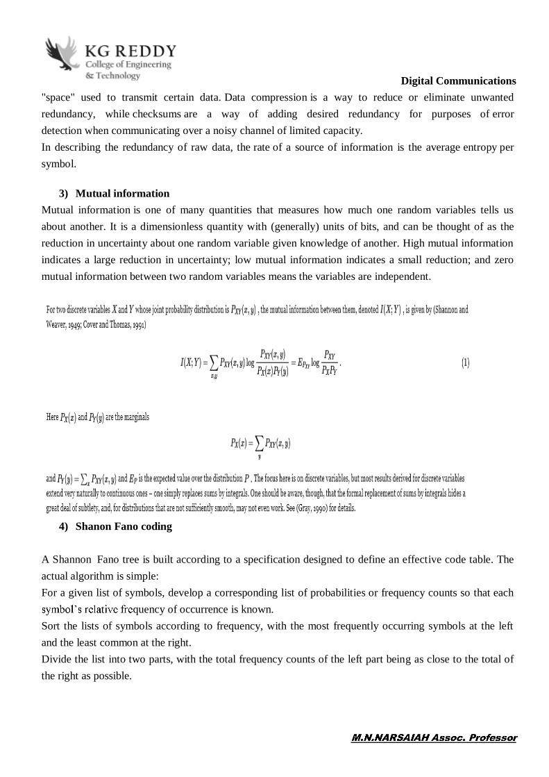
3) Mutual information Mutual information is one of many quantities that measures how much one random variables tells us about another. It is a dimensionless quantity with (generally) units of bits, and can be thought of as the reduction in uncertainty about one random variable given knowledge of another. High mutual information indicates a large reduction in uncertainty; low mutual information indicates a small reduction; and zero mutual information between two random variables means the variables are independent.
4) Shanon Fano coding
A Shannon Fano tree is built according to a specification designed to define an effective code table. The actual algorithm is simple: For a given list of symbols, develop a corresponding list of probabilities or frequency counts so that each
quency of occurrence is known. Sort the lists of symbols according to frequency, with the most frequently occurring symbols at the left and the least common at the right. Divide the list into two parts, with the total frequency counts of the left part being as close to the total of the right as possible.

Digital CommunicationsThe left part of the list is assigned the binary digit 0, and the right part is assigned the digit 1. This means that the codes for the symbols in the first part will all start with 0, and the codes in the second part will all start with 1. Recursively apply the steps 3 and 4 to each of the two halves, subdividing groups and adding bits to the codes until each symbol has become a corresponding code leaf on the tree. Example[edit]
Shannon Fano Algorithm The example shows the construction of the Shannon code for a small alphabet. The five symbols which can be coded have the following frequency:
Symbol A B C D E
Count 15 7 6 6 5
Probabilities 0.38461538 0.17948718 0.15384615 0.15384615 0.12820513
All symbols are sorted by frequency, from left to right (shown in Figure a). Putting the dividing line between symbols B and C results in a total of 22 in the left group and a total of 17 in the right group. This minimizes the difference in totals between the two groups. With this division, A and B will each have a code that starts with a 0 bit, and the C, D, and E codes will all start with a 1, as shown in Figure b. Subsequently, the left half of the tree gets a new division between A and B, which puts A on a leaf with code 00 and B on a leaf with code 01.

Digital CommunicationsAfter four division procedures, a tree of codes results. In the final tree, the three symbols with the highest frequencies have all been assigned 2-bit codes, and two symbols with lower counts have 3-bit codes as shown table below:
Symbol A B C D E
Code 00 01 10 110 111
Results in 2 bits for A, B and C and per 3 bits for D and E an average bit number of { {\ {2{bits}}\* (15+7+6)+3\,{bits}}\cdot (6+5)}{39\,{\text{symbols}}}}\=2.28{bits per symbol.}}}
5) Information loss due to noise Let P(message)=P('i') (i.e. the a priori probability).Information transmitted =log2 (1/P('i')) bits Assume noisy channel where P('i'| V) denotes the a posteriori (reception) probability. Then to account for lost information due to incorrect decisions we say that the information received
If there is no noise then P('i'| v) = 1 and information received equals information transmitted, i.e. for no noise there is no loss of information. If noise is present then P('i'I v) is less than 1 and information is lost.
3. FIVE MARKS QUESTION WITH ANSWERS
1) Define and explain Huffman code Huffman code is a particular type of optimal prefix code that is commonly used for lossless data compression. The process of finding and/or using such a code proceeds by means of Huffman coding, an algorithm developed by David A. Huffman while he was a Sc.D. student at MIT, and published in the 1952 paper "A Method for the Construction of Minimum-Redundancy Codes". The output from Huffman's algorithm can be viewed as a variable-length code table for encoding a source symbol (such as a character in a file). The algorithm derives this table from the estimated probability or frequency of occurrence (weight) for each possible value of the source symbol. As in other entropy encoding methods, more common symbols are generally represented using fewer bits than less common symbols. Huffman's method can be efficiently implemented, finding a code in time linear to the number of input weights if these weights are sorted. However, although optimal among methods encoding symbols separately, Huffman coding is not always optimal among all compression methods.

Digital Communications a very simple
their frequencies, into a new symbol. We do this repeatedly until we only have one symbol. The result is a
symbols {a,b,c,d,e,o, k} with differing probabilities (Figure 1). The codeword for each symbol is the sequences of left (0) and right (1) moves required to reach that symbol from the top of the tree. Notice that in this example we have 7 symbols, so the naive fixed-length code would require 3 bits per symbol ( 2 8 7 3 = ! ). The Huffman code (which is variable-length) requires on average 2.48 bits; while the entropy gives a lower bound of 2.41 bits. The fact that it is a prefix code makes it easy to decode a string symbol by symbol by starting from the top of the tree and moving down left or right every time a new bit arrives. For example, try decoding: 1010011010010100.
2) Define and explain Variable length coding In coding theory a variable-length code is a code which maps source symbols to a variable number of bits. Variable-length codes can allow sources to be compressed and decompressed with zero error (lossless data compression) and still be read back symbol by symbol. With the right coding strategy an independent and identically-distributed source may be compressed almost arbitrarily close to its entropy. This is in contrast to fixed length coding methods, for which data compression is only possible for large blocks of

Digital Communicationsdata, and any compression beyond the logarithm of the total number of possibilities comes with a finite (though perhaps arbitrarily small) probability of failure. Some examples of well-known variable-length coding strategies are Huffman coding, Lempel Ziv coding and arithmetic coding. Codes and their extensions The extension of a code is the mapping of finite length source sequences to finite length bit strings, that is obtained by concatenating for each symbol of the source sequence the corresponding codeword produced by the original code. Using terms from formal language theory, the precise mathematical definition is as follows: Let {S} and {T} be two finite sets, called the source and target alphabets, respectively. A code {\ C:S\to
T^{*}} is a total function mapping each symbol from {S} to a sequence of symbols over {T},and the
extension of {C} to a homomorphism of {S^{*}} T^{*}}which naturally maps each sequence of source symbols to a sequence of target symbols, is referred to as its extension. Classes of variable-length codes[edit] Variable-length codes can be strictly nested in order of decreasing generality as non-singular codes, uniquely decodable codes and prefix codes. Prefix codes are always uniquely decodable, and these in turn are always non-singular: Non-singular codes A code is non-singular if each source symbol is mapped to a different non-empty bit string, i.e. the mapping from source symbols to bit strings is injective. For example the mapping is not non-singular because both "a" and "b" map to the same bit string "0" ; any extension of this mapping will generate a lossy (non-lossless) coding. Such singular coding may still be useful when some loss of information is acceptable (for example when such code is used in audio or video compression, where a lossy coding becomes equivalent to source quantization). However, the mapping is non-singular ; its extension will generate a lossless coding, which will be useful for general data transmission (but this feature is not always required). Note that it is not necessary for the non-singular code to be more compact than the source (and in many applications, a larger code is useful, for example as a way to detect and/or recover from encoding or transmission errors, or in security applications to protect a source from undetectable tampering). Uniquely decodable codes A code is uniquely decodable if its extension is non-singular (see above). Whether a given code is uniquely decodable can be decided with the Sardinas Patterson algorithm. The mapping is uniquely decodable (this can be demonstrated by looking at the follow-set after each target bit string in the map, because each bit string is terminated as soon as we see a 0 bit which cannot follow any existing code to create a longer valid code in the map, but unambiguously starts a new code). Consider again the code from the previous section. This code, which is based on an example found in,[1] is not uniquely decodable, since the string 011101110011 can be interpreted as the sequence of

Digital Communications 01110 1110 011 1 011 10011. Two
possible decoding of this encoded string are thus given by cdb and babe. However, such a code is useful when the set of all possible source symbols is completely known and finite, or when there are restrictions (for example a formal syntax) that determine if source elements of this extension are acceptable. Such restrictions permit the decoding of the original message by checking which of the possible source symbols mapped to the same symbol are valid under those restrictions. Main article: Prefix code A code is a prefix code if no target bit string in the mapping is a prefix of the target bit string of a different source symbol in the same mapping. This means that symbols can be decoded instantaneously after their entire codeword is received. Other commonly used names for this concept are prefix-free code, instantaneous code, or context-free code. The example mapping M_{3} in the previous paragraph is not a prefix code because we don't know after reading the bit string "0" if it encodes an "a" source symbol, or if it is the prefix of the encodings of the "b" or "c" symbols. An example of a prefix code is shown below.
Symbol Codeword
a 0
b 10
c 110
d 111
Example of encoding and decoding:
A special case of prefix codes are block codesare not very useful in the context of source coding, but often serve as error correcting codes in the context of channel coding. Another special case of prefix codes are variable-length quantity codes, which encode arbitrarily large integers as a sequence of octets -- i.e., every codeword is a multiple of 8 bits. Advantages The advantage of a variable-length code is that unlikely source symbols can be assigned longer codewords
expected codeword length.
3) Define and explain Lossy source coding Sometimes it might be too expensive to reconstruct the source in a lossless way. Sometimes it is impossible to reconstruct the source losslessly. For example, if the source is continuous-valued, the entropy rate of the source is usually infinite! Lossy source coding has wide range of applications, including quantization/digitization of continuous-valued signals, image/video/audio compression, etc. In

Digital Communicationsthis lecture, we first focus on discrete memory less sources (DMS). Then, we employ the discretization technique to extend the coding theorems from the discrete-source case to the continuous-source case. In particular, Gaussian sources will be our main focus.

Digital Communications

Digital Communications
4) Define and explain Source coding to increase average information Introduction: · An important problem in communications is the efficient representation of data generated by a discrete source. The process by which this representation is accomplished is called source encoding. The device that performs the representation is called a source encoder. · For the source encoder to be efficient, we require knowledge of the statistics of the source. In particular, if some source symbols are known to be more probable than others, then we may exploit this feature in the generation of a source code by assigning short code words to frequent source symbols, and long code words to rare source symbols. · We refer to such a source code as a variable-length code. The Morse code is an example of a variable_ length code. In the Morse code, the letters of the alphabet and numerals are encoded into streams of marks and spaces, denoted as dots "." and dashes "-" , respectively. · Our primary interest is in the development of an efficient source encoder that satisfies two functional requirements: 1. The code words produced by the encoder are in binary form. 2. The source code is uniquely decodable, so that the original source sequence can be reconstructed perfectly from the encoded binary sequence. · Source coding does not change or alter the source entropy, i.e. the average number of information bits per source symbol. In this sense source entropy is a fundamental property of the source. Source coding, however, alter (usually increase) the entropy of the source coded symbols. It may also reduce fluctuations in the information rate from the source and avoid symbol 'surges' which could overload the channel when the message sequence contains many high probability (i.e. frequently occurring, low entropy) symbols.

Digital Communications
For a set of symbols represented by binary code words with lengths lm (binary) digits, an overall code length, L, can be defined as the average codeword length, i.e

Digital Communications4. OBJECTIVE QUESTIONS WITH ANSWERS
Q1. For a (7, 4) block code, 7 is the total number of bits and 4 is the number of a) Information bits b) Redundant bits c) Total bits- information bits d) None of the above
ANSWER: a) Information bits Q2. Interleaving process permits a burst of B bits, with l as consecutive code bits and t errors when a) B <= 2tl b) B >= tl c) B <= tl/2 d) B <= tl
ANSWER: d) B <= tl
Q3. The code in convolution coding is generated using a) EX-OR logic b) AND logic c) OR logic d) None of the above
ANSWER: a) EX-OR logic Q4. For decoding in convolution coding, in a code tree, a) Diverge upward when a bit is 0 and diverge downward when the bit is 1 b) Diverge downward when a bit is 0 and diverge upward when the bit is 1 c) Diverge left when a bit is 0 and diverge right when the bit is 1 d) Diverge right when a bit is 0 and diverge left when the bit is 1 ANSWER: a) Diverge upward when a bit is 0 and diverge downward when the bit is 1
Digital Communications Q5. A linear code a) Sum of code words is also a code word b) All- zero code word is a code word c) Minimum hamming distance between two code words is equal to weight of any non zero code word d) All of the above
ANSWER: d) All of the above Q6. Graphical representation of linear block code is known as a) Pi graph b) Matrix c) Tanner graph d) None of the above ANSWER: c) Tanner graph
Q7. Orthogonality of two codes means a) The integrated product of two different code words is zero b) The integrated product of two different code words is one c) The integrated product of two same code words is zero d) None of the above Q8. The Golay code (23,12) is a codeword of length 23 which may correct a) 2 errors b) 3 errors c) 5 errors d) 8 errors ANSWER: b) 3 errors Q9. The minimum distance for unextended Golay code is a) 8 b) 9 c) 7 d) 6 ANSWER: c) 7

Digital Communications Q10. The prefix code is also known as a) Instantaneous code b) Block code c) Convolution code d) Parity bit
ANSWER: a) Instantaneous code Q11. Run Length Encoding is used for a) Reducing the repeated string of characters b) Bit error correction c) Correction of error in multiple bits d) All of the above ANSWER: a) Reducing the repeated string of characters
5. FILL IN THE BLANK QUESTIONS WITH ANSWERS
1) ------------ aims at developing methods for coding to check the correctness of the bit stream transmitted.
2) -------------, a code is linear if two codes are added using modulo-2 arithmetic produces a third codeword in the code.
3) All error patterns that differ by a codeword have the same ---------. 4) ---------, d (c1, c2) between two code words c1 and c2 is defined as the number of bits in which
they differ. 5) Cyclic property: Any cyclic shift of a codeword in the code is also a --------. 6) ---------- code is a type of error-correcting code that generates parity symbols via the sliding
application of a boolean polynomial function to a data stream 7) A convolution encoder is a ------ machine. 8) ------- is a block code , where the circular shifts of each codeword gives another word that belongs
to the code. They are error-correcting codes that have algebraic properties that are convenient for efficient error detection and correction.
9) ---------- is an error-correcting code for which any linear combination of code words is also a codeword.
10) --------- is a dynamic programming algorithm for finding the most likely sequence of hidden states called the Viterbi path that results in a sequence of observed events, especially in the context of Markov information sources and hidden Markov models.
Ans: 1) Error control coding

Digital Communications2) Linear block code 3) Syndrome 4) Hamming distance 5) Codeword 6) convolution code 7) finite state 8) cyclic code 9) linear code 10) The Viterbi algorithm

Digital CommunicationsUNIT3
1. TWO MARKS QUESTION WITH ANSWERS
1) Define Probability of error In statistics, the term "error" arises in two ways. Firstly, it arises in the context of decision making, where the probability of error may be considered as being the probability of making a wrong decision and which would have a different value for each type of error. Secondly, it arises in the context of statistical modelling (for example regression) where the model's predicted value may be in error regarding the observed outcome and where the term probability of error may refer to the probabilities of various amounts of error occurring.
2) Define Optimum receiver A receiver is said to be optimum if it yields the minimum probability of error Pe . We assume that additive white Gaussian noise (AWGN) is the only system perturbance, and that the bandwidth is not constrained; that is, an infinite bandwidth inter symbol-interference-free transmission channel is available. The derivation that follows and the suggested implementation methods apply to baseband and to coherent binary modulated systems in general.
3) Define Pulse shaping of optimum transmission In electronics and telecommunications, pulse shaping is the process of changing the waveform of transmitted pulses. Its purpose is to make the transmitted signal better suited to its purpose or the communication channel, typically by limiting the effective bandwidth of the transmission. By filtering the transmitted pulses this way, the intersymbol interference caused by the channel can be kept in control. In RF communication, pulse shaping is essential for making the signal fit in its frequency band. Typically pulse shaping occurs after line coding and modulation.
4) Draw EYE diagram for ASK, FSK,PSK

Digital Communications
5) Define Intersymbol interference: Intersymbol interference (ISI) is a form of distortion of a signal in which one symbol interferes with
subsequent symbols. This is an unwanted phenomenon as the previous symbols have similar effect
as noise, thus making the communication less reliable. The spreading of the pulse beyond its allotted time
interval causes it to interfere with neighboring pulses.[1] ISI is usually caused by multipath propagation or
the inherent linear or non-linear frequency response of a communication channel causing successive
symbols to "blur" together.
The presence of ISI in the system introduces errors in the decision device at the receiver output. Therefore,
in the design of the transmitting and receiving filters, the objective is to minimize the effects of ISI, and
thereby deliver the digital data to its destination with the smallest error rate possible.
Ways to alleviate intersymbol interference include adaptive equalization and error correcting codes.
2. THREE MARKS QUESTION WITH ANSWERS
1) Explain Eye pattern Eye Pattern:
In telecommunication, an eye pattern, also known as an eye diagram, is an oscilloscope display in which a digital signal from a receiver is repetitively sampled and applied to the vertical input, while the data rate is used to trigger the horizontal sweep. It is so called because, for several types of coding, the pattern looks like a series of eyes between a pair of rails. It is a tool for the evaluation of the combined effects of channel noise and intersymbol interference on the performance of a baseband pulse-transmission system. It is the synchronized superposition of all possible realizations of the signal of interest viewed within a particular signaling interval. Several system performance measures can be derived by analyzing the display. If the signals are too long, too short, poorly synchronized with the system clock, too high, too low, too noisy, or too slow to change, or have too much undershoot or overshoot, this can be observed from the eye diagram. An open eye pattern corresponds to minimal signal distortion. Distortion of the signal waveform due to intersymbol interference and noise appears as closure of the eye pattern
Example
The eye diagram of a binary PSK system

Digital Communications
The eye diagram of the same system with multipath interference(MI) effects added
Eye diagram of a 4 level PAM signal
Measurements
There are many measurements that can be obtained from an eye diagram:[4]
Amplitude measurements
Eye amplitude Eye crossing amplitude Eye crossing percentage Eye height Eye level Eye signal-to-noise ratio Quality factor Vertical eye opening
Time measurements
Deterministic jitter Eye crossing time Eye delay Eye fall time Eye rise time Eye width Horizontal eye opening Peak-to-peak jitter Random jitter RMS jitter CRC jitter Total jitter
Interpreting measurements
Eye-diagram feature What it measures

Digital Communications
Eye opening (height, peak to peak) Additive noise in the signal
Eye overshoot/undershoot Peak distortion due to interruptions in the signal path
Eye width Timing synchronization & jitter effects
Eye closure Intersymbol interference, additive noise
2) Explain Nyquist criterion for baseband transmission:

Digital Communications
3) Explain Digital subscriber line
Digital subscriber line (DSL; originally digital subscriber loop) is a family of technologies that are used
to transmit digital data over telephone lines. In telecommunications marketing, the term DSL is widely
understood to mean asymmetric digital subscriber line(ADSL), the most commonly installed DSL
technology, for Internet access. DSL service can be delivered simultaneously with wired telephone
service on the same telephone line since DSL uses higher frequency bands for data. On the customer
premises, a DSL filteron each non-DSL outlet blocks any high-frequency interference to enable
simultaneous use of the voice and DSL services.
The bit rate of consumer DSL services typically ranges from 256 kbit/s to over 100 Mbit/s in the direction
to the customer (downstream), depending on DSL technology, line conditions, and service-level
implementation. Bit rates of 1 Gbit/s have been reached in trials,[1] but most homes are likely to be limited
to 500-800 Mbit/s. In ADSL, the data throughput in the upstream direction (the direction to the service
provider) is lower, hence the designation of asymmetric service. In symmetric digital subscriber

Digital Communicationsline (SDSL) services, the downstream and upstream data rates are equal. Researchers at Bell Labs have
reached speeds of 10 Gbit/s, while delivering 1 Gbit/s symmetrical broadband access services using
traditional copper telephone lines.
4) Explain Optimal line receiver
5) Explain Adaptive equalization
An adaptive equalizer is an equalizer that automatically adapts to time-varying properties of the communication channel. It is frequently used with coherent modulations such as phase shift keying, mitigating the effects of multipath propagation and Doppler spreading.
Many adaptation strategies exist. They include:
LMS Note that the receiver does not have access to the transmitted signal x when it is not in training mode. If the probability that the equalizer makes a mistake is sufficiently small, the symbol decisions d(n) made by the equalizer may be substituted for x
RLS
A well-known example is the decision feedback equalizer, a filter that uses feedback of detected symbols in addition to conventional equalization of future symbols. Some systems use predefined training sequences to provide reference points for the adaptation process.

Digital Communications
3. FIVE MARKS QUESTION WITH ANSWERS
1) Explain BASEBAND M-ARY PAM TRANSMISSION
Partial response signalling (PRS), also known as correlative coding, was introduced for the first time in
1960s for high data rate communication [lender, 1960]. From a practical point of view, the background of
this technique is related to the Nyquist criterion.
Assume a Pulse Amplitude Modulation (PAM), according to the Nyquist criterion, the highest possible
transmission rate without Inter-symbol-interference (ISI) at the receiver over a channel with a bandwidth of
W (Hz) is 2W symbols/sec.
BASEBAND M-ARY PAM TRANSMISSION
Up to now for binary systems the pulses have two possible amplitude levels. In a baseband M-ary PAM
system, the pulse amplitude modulator produces M possible amplitude levels with M>2. In an M-ary
system, the information source emits a sequence of symbols from an alphabet that consists of M symbols.
Each amplitude level at the PAM modulator output corresponds to a distinct symbol. The symbol duration
T is also called as the signaling rate of the system, which is expressed as symbols per second or bauds.
consists of two bits.
The symbol duration T of the M-ary system is related to the bit duration Tb of the equivalent binary PAM
system as For a given channel bandwidth, using M-ary PAM system, log2M times more information is
transmitted than binary PAM system. T = Tb log2 M transmitted than binary PAM system. The price we
paid is the increased bit error rate compared binary PAM system. To achieve the same probability of error
as the binary PAM system, the transmit power in <-ary PAM system must be increased.
For M much larger than 2 and an average probability of symbol error small compared to 1, the transmitted
power must be increased by a factor of M2/log2M compared to binary PAM system. The M-ary PAM
transmitter and receiver is similar to the binary PAM transmitter and receiver. In transmitter, the M-ary
pulse train is shaped by a transmit filter and transmitted through a channel which corrupts the signal with
noise and ISI. The received signal is passed through a receive filter and sampled at an appropriate rate in
synchronism with the transmitter. Each sample is compared with preset threshold values and a decision is
made as to which symbol was transmitted. Obviously, in M-ary system there are M-1 threshold levels
which makes the system complicated.
2) Explain Gram-Schmidt orthogonalization procedure
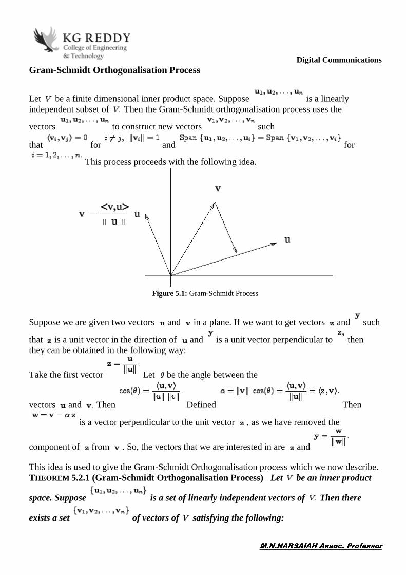
Digital CommunicationsGram-Schmidt Orthogonalisation Process
Let be a finite dimensional inner product space. Suppose is a linearly independent subset of Then the Gram-Schmidt orthogonalisation process uses the
vectors to construct new vectors such
that for and for
This process proceeds with the following idea.
Figure 5.1: Gram-Schmidt Process
Suppose we are given two vectors and in a plane. If we want to get vectors and such
that is a unit vector in the direction of and is a unit vector perpendicular to then they can be obtained in the following way:
Take the first vector Let be the angle between the
vectors and Then Defined Then
is a vector perpendicular to the unit vector , as we have removed the
component of from . So, the vectors that we are interested in are and
This idea is used to give the Gram-Schmidt Orthogonalisation process which we now describe. THEOREM 5.2.1 (Gram-Schmidt Orthogonalisation Process) Let be an inner product
space. Suppose is a set of linearly independent vectors of Then there
exists a set of vectors of satisfying the following:

Digital Communications
1. for
2. for and
3. for
Proof. We successively define the vectors as follows.
Calculate and let
Obtain and let
In general, if are already obtained, we compute
(5.2.1)
and define
We prove the theorem by induction on the number of linearly independent vectors.
For we have Since and
Hence, the result holds for
Let the result hold for all That is, suppose we are given any set
of linearly independent vectors of Then by the inductive
assumption, there exists a set of vectors satisfying the following:
1. for
2. for and

Digital Communications
3. for
Now, let us assume that we are given a set of linearly independent
vectors of Then by the inductive assumption, we already have
vectors satisfying
1. for
2. for and
3. for Using (5.2.1), we define
(5.2.2)
We first show that . This will also imply that and
hence is well defined.
On the contrary, assume that Then there exist
scalars such that
So, by (5.2.2)
Thus, by the third induction assumption,
This gives a contradiction to the given assumption that the set of vectors is linear independent.
So, . Define . Then . Also, it can be easily verified
that for . Hence, by the principle of mathematical induction, the proof of the theorem is complete. height6pt width 6pt depth 0pt

Digital CommunicationsWe illustrate the Gram-Schmidt process by the following example.
Let be a linearly independent set in Find an
orthonormal set such that
Solution: Let Define Let Then
Hence, Let Then
and
1. Let be any basis of a -dimensional subspace of Then by Gram-Schmidt orthogonalisation process, we get an orthonormal
set with and for
2. Suppose we are given a set of vectors, of that are linearly
dependent. Then by Corollary 3.2.5, there exists a smallest such that
We claim that in this case,
Since, we have chosen the smallest satisfying

Digital Communications
for the set is linearly independent (use Corollary 3.2.5).
So, by Theorem 5.2.1, there exists an orthonormal set such that
As by Remark 5.1.15
So, by definition of
Therefore, in this case, we can continue with the Gram-Schmidt process by
replacing by
3. Let be a countably infinite set of linearly independent vectors. Then one can apply the Gram-Schmidt process to get a countably infinite orthonormal set.
4. Let be an orthonormal subset of Let be the standard ordered basis of Then there exist real
numbers such that
Let Then in the ordered basis we have
is an matrix.

Digital Communications
Also, observe that the conditions and for implies that
(5.2.3)
Note that,
Or using (5.2.3), in the language of matrices, we get
Perhaps the readers must have noticed that the inverse of is its transpose. Such matrices are called orthogonal matrices and they have a special role to play.
DEFINITION 5.2.4 (Orthogonal Matrix) A real matrix is said to be an orthogonal
matrix if
It is worthwhile to solve the following exercises. EXERCISE 5.2.5

Digital Communications1. Let and be two n*n orthogonal matrices. Then prove that and are both
orthogonal matrices.
2. Let be an orthogonal matrix. Then prove that 1. the rows of form an orthonormal basis of 2. the columns of form an orthonormal basis of
3. for any two vectors
4. for any vector
3. Let be an orthonormal basis of Let be the
standard basis of Construct an matrix by
where
Prove that Hence deduce that is an orthogonal matrix.
4. Let be an upper triangular matrix. If is also an orthogonal matrix, then
prove that THEOREM 5.2.6 (QR Decomposition) Let be a square matrix of order Then there
exist matrices and such that is orthogonal and is upper triangular with
In case, is non-singular, the diagonal entries of can be chosen to be positive. Also, in this case, the decomposition is unique. Proof. We prove the theorem when is non-singular. The proof for the singular case is left as an exercise.

Digital Communications
Let the columns of be The Gram-Schmidt orthogonalisation process applied
to the vectors gives the vectors satisfying
(5.2.4)
Now, consider the ordered basis From (5.2.4), for we
have So, we can find scalars such that
(5.2.5)
Let Then by Exercise 5.2.5.3, is an orthogonal matrix. We now define
an upper triangular matrix by
By using (5.2.5), we get
Thus, we see that where is an orthogonal matrix (see Remark 5.2.3.4) and is an upper triangular matrix.

Digital Communications
The proof doesn't guarantee that for is positive. But this can be achieved by
replacing the vector by whenever is negative.
Uniqueness: suppose then Observe the following properties of upper triangular matrices.
1. The inverse of an upper triangular matrix is also an upper triangular matrix, and 2. product of upper triangular matrices is also upper triangular.
Thus the matrix is an upper triangular matrix. Also, by Exercise 5.2.5.1, the
matrix is an orthogonal matrix. Hence, by
Exercise 5.2.5.4, So, and therefore height6pt width 6pt depth 0pt
Suppose we have matrix of dimension with Then by Remark 5.2.3.2, the application of the Gram-Schmidt orthogonalisation process yields a
set of orthonormal vectors of In this case, for each we have
Hence, proceeding on the lines of the above theorem, we have the following result.
THEOREM 5.2.7 (Generalised QR Decomposition) Let be an matrix of
rank Then where
1. is an matrix with That is, the columns of form an orthonormal set,
2. If then and
3. is an matrix with
3) Explain Matched filter

Digital CommunicationsIn signal processing, a matched filter is obtained by correlating a known signal, or template, with an
unknown signal to detect the presence of the template in the unknown signal.[1][2] This is equivalent to
convolving the unknown signal with a conjugated time-reversed version of the template. The matched filter
is the optimal linear filter for maximizing the signal to noise ratio (SNR) in the presence of additive
stochastic noise. Matched filters are commonly used in radar, in which a known signal is sent out, and the
reflected signal is examined for common elements of the out-going signal. Pulse compression is an
example of matched filtering. It is so called because impulse response is matched to input pulse signals.
Two-dimensional matched filters are commonly used in image processing, e.g., to improve SNR for X-ray.
Matched filtering is a demodulation technique with LTI (linear time invariant) filters to maximize SNR.[3]
It was originally also known as a North filter.
MATCHED FILTER
the interval 0<t<T. we can design a linear filter with impulse response hj(t), with the received signal x(t)
the fitter output is given by the convolution integral
where xj is the j th correlator output produced by the received signal x(t).
A filter whose impulse response is time-reversed and delayed version of the input signal is said to be
matched. Correspondingly , the optimum receiver based on this is referred as the matched filter receiver.
For a matched filter operating in real time to be physically realizable, it must be causal. For causal system

Digital Communications
h(t) = impulse response W(t) =white noise
The impulse response of the matched filter is time-reversed and delayed version of the input signal.
4) Explain Geometric interpretation of signals

Digital Communications
Basis Vectors The set of basis vectors {e1, e en} of a space are chosen such that: Should be complete or span the vector space: any vector a can be expressed as a linear combination of these vectors. Each basis vector should be orthogonal to all others · Each basis vector should be normalized: · A set of basis vectors satisfying these properties is also said to be a complete orthonormal basis · In an n-dim space, we can have at most n basis vectors
Signal Space Basic Idea: If a signal can be represented by n-tuple, then it can be treated in much the same way as a n-dim vector.
n signals Consider a signal x(t) and suppose that If every signal can be written as above ~ ~ basisfunctions and we have a n-dim signal space

Digital CommunicationsOrthonormal Basis
orthogonal set if
Then, we can express each of these waveforms as weighted linear combination of orthonormal signals
Let, for a convenient set of {
Now, we can represent a signal si(t) as a column vector whose elements are the scalar coefficients
These M energy signals or vectors can be viewed as a set of M points in an N dimensional
Sig .Signal Constellation is the collection of M signals points (or messages) on the signal space
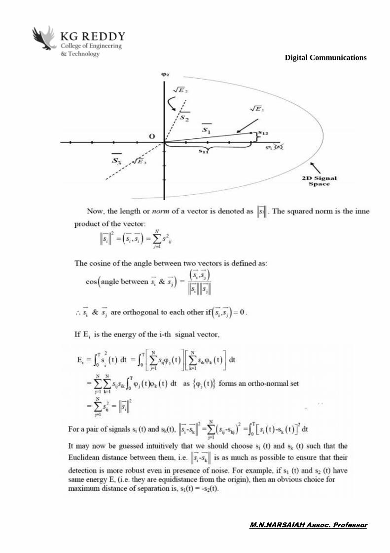
Digital Communications

Digital Communications5) Explain Probability of error
In a binary PCM system, binary digits may be represented by two pulse levels. If these levels are chosen to
be 0 and A, the signal is termed an on-off binary signal. If the level switches between -A=2 and+ A=2 it is
called a polar binary signal. Suppose we are transmitting digital information, and decide to do this using
Two-level pulses each with

Digital Communications

Digital Communications

Digital Communications

Digital Communications4. OBJECTIVE QUESTIONS WITH ANSWERS
1)In discrete memory less source, the current letter produced by a source is statistically independent of _____
a. Past output b. Future output c. Both a & b d. None of the above ANSWER: Both a and b
2)Which coding terminology deals with the inverse operation of assigned words of second language corresponding to the words in the first language? a. Enciphering b. Deciphering c. Codeword d. Codebook ANSWER: Deciphering
3)Huffman coding technique is adopted for constructing the source code with ________ redundancy. a. Maximum b. Constant c. Minimum d. Unpredictable ANSWER: Minimum 4) Which bitmap file format/s support/s the Run Length Encoding (RLE)? a. TIFF b. BMP c. PCX d. All of the above
ANSWER: All of the above
5) In dictionary techniques for data compaction, which approach of building dictionary is used for the prior knowledge of probability of the frequently occurring patterns?
a. Static Dictionary

Digital Communicationsb. Adaptive Dictionary c. Both a & b d. None of the above ANSWER: Static Dictionary
6) Which type of channel does not represent any correlation between input and output Symbols?
a. Noiseless Channel b. Lossless Channel c. Useless Channel d. Deterministic Channel ANSWER: Useless Channel
7) In digital communication system, smaller the code rate, _________are the redundant bits. a. less b. more c. equal d. unpredictable ANSWER: more
8) In channel coding theorem, channel capacity decides the _________permissible rate at which error free transmission is possible.
a. Maximum b. Minimum c. Constant d. None of the above ANSWER: Maximum
9) If the channel is bandlimited to 6 kHz & signal to noise ratio is 16, what would be the capacity of channel?
a. 15.15 kbps b. 24.74 kbps c. 30.12 kbps d. 52.18 kbps ANSWER: 24.74 kbps

Digital Communications10) According to Shannon's second theorem, it is not feasible to transmit information
over the channel with ______error probability, although by using any coding technique. a. small b. large c. stable d. unpredictable answer : small
4. FILL IN THE BLANK QUESTIONS WITH ANSWERS 1) ------------- studies the quantification, storage, and communication of information. 2) A key measure in information theory is "-----------" 3) Information theory is based on ------------ and ---------. 4) The ----------- of two discrete random variables X and Y is merely the entropy of their
pairing: (X, Y). this implies that if X and Y are independent, then their joint entropy is the sum of their individual entropies.
5) -------------- measures the amount of information that can be obtained about one random variable by observing another. It is important in communication where it can be used to maximize the amount of information shared between sent and received signals.
6) ------------- is one of the most important and direct applications of information theory. 7) ------------ is the process of converting binary data, a sequence of bits to a digital signal. 8) ------- involves transmission of extra bits along with the data bits. 9) ----------- is a particular type of optimal prefix code that is commonly used for lossless data
compression. 10) ------------ , the symbols are arranged in order from most probable to least probable, and then
divided into two sets whose total probabilities are as close as possible to being equal.
Ans: 1) Information theory 2) Entropy 3) Probability theory and statistics. 4) The joint entropy 5) Mutual information 6) Coding theory 7) Line code 8) Redundancy 9) Huffman code 10) In Shannon Fano coding

Digital CommunicationsUNIT 4
2 marks 5 questions with answer 1) What is meant by coherent detection system? In coherent ASK, correlation receiver is used to detect the signal. Locally generated carrier is correlated with incoming Ask signal. The locally generated carrier is in exact phase either transmitted carrier. Coherent Ask is also called synchronous ASK. 2) Why is PSK always preferable over ASK in coherent detection? ASK is on-off signaling where as the modulated carrier is continuously transmitted in PSK. Hence peak power requirement is more in ASK, where it is reduces in PSK. 3) Differentiate between coherent and non-coherent detection In coherent detection the local carrier generated at the receiver is phase locked with the carrier at the transmitter. Hence it is also called synchronous detection. In non coherent detection the local carrier generated at the receiver not be phase locked with the carrier at the transmitter. It is simple, but it has higher probability of error. 4) What are the drawbacks of binary PSK system? It is difficult to detect +b(t) and b(t) because of squaring in the receiver Problem, of ISI and inter channel interference are present. 5) What is the average bit error probability? A BPSK system makes errors at the average rate of 1000 errors per delay. Data rate is 1 kbps the single-sided noise power spectral density is 10-20 W/Hz. Assuming the system to be wide sense stationary, 24*60*60=86400sec 86.4*106 Bit error probability Pe=100/86.4*106 =1.1157*10-6
3. THREE MARKS QUESTIONS WITH ANSWER 1) What is meant by DPSK? In DPSK, the input sequence is modified. Let input sequence be d(t) and output Sequence be b(t). Sequence b(t) changes level at the beginning of each interval in which d(t)=1 and it does not changes level when d(t)=0. When b(t) changes level, phase of the carrier is changed. And as stated above, b(t) changes t=its level only when d(t) =1. This means phase of the carrier is changed only if d(t)=1. Hence the technique is called Differential PSK.

Digital Communications2) Define QPSK. In QPSK two successive bits in the data sequence are grouped together. This combination of two bits forms four distinct symbols. When the symbol is changed to next symbol the phase of the carrier is
Because of combination of two bits there will be four symbols. Hence
QPSK reduces amplitude variations and required transmission bandwidth.
3) Explain ASK Modulator Amplitude-shift keying (ASK) is a form of amplitude modulation that represents digital data as variations in the amplitude of a carrier wave. In an ASK system, the binary symbol 1 is represented by transmitting a fixed-amplitude carrier wave and fixed frequency for a bit duration of T seconds. If the signal value is 1 then the carrier signal will be transmitted; otherwise, a signal value of 0 will be transmitted. Any digital modulation scheme uses a finite number of distinct signals to represent digital data. ASK uses a finite number of amplitudes, each assigned a unique pattern of binary digits. Usually, each amplitude encodes an equal number of bits. Each pattern of bits forms the symbol that is represented by the particular amplitude. The demodulator, which is designed specifically for the symbol-set used by the modulator, determines the amplitude of the received signal and maps it back to the symbol it represents, thus recovering the original data. Frequency and phase of the carrier are kept constant.
4) Define FSK Frequency-shift keying (FSK) is a frequency modulation scheme in which digital information is transmitted through discrete frequency changes of a carrier signal.[1] The technology is used for communication systems such as amateur radio, caller ID and emergency broadcasts. The simplest FSK is binary FSK (BFSK). BFSK uses a pair of discrete frequencies to transmit binary (0s and 1s) information.[2] With this scheme, the "1" is called the mark frequency and the "0" is called the space frequency. 5) Explain Frequency spectrum of FSK
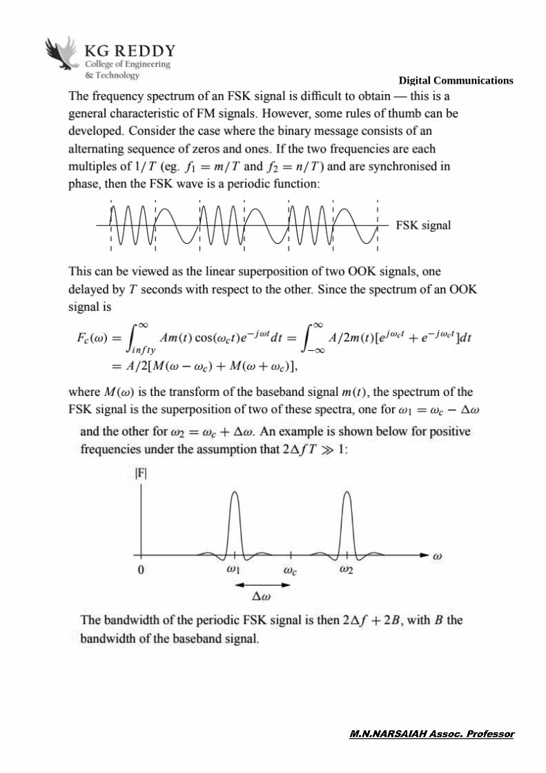
Digital Communications

Digital Communications3. FIVE MARKS QUESTIONS WITH ANSWER
1) Explain Coherent and non coherent ASK detector Amplitude-shift keying (ASK) is a form of amplitude modulation that represents digital data as variations in the amplitude of a carrier wave. In an ASK system, the binary symbol 1 is represented by transmitting a fixed-amplitude carrier wave and fixed frequency for a bit duration of T seconds. If the signal value is 1 then the carrier signal will be transmitted; otherwise, a signal value of 0 will be transmitted. Any digital modulation scheme uses a finite number of distinct signals to represent digital data. ASK uses a finite number of amplitudes, each assigned a unique pattern of binary digits. Usually, each amplitude encodes an equal number of bits. Each pattern of bits forms the symbol that is represented by the particular amplitude. The demodulator, which is designed specifically for the symbol-set used by the modulator, determines the amplitude of the received signal and maps it back to the symbol it represents, thus recovering the original data. Frequency and phase of the carrier are kept constant.
In transmitter the binary data sequence is given to an on- ff enc der. This gives an output Eb volts for symbol 1 and 0 volt for symbol 0. The resulting binary wave [in Unipolar form] and sinusoidal carrier
1 (t) are applied to a product modulator. The desired BASK wave is obtained at the modulator output.
In demodulator, the received noisy BASK signal x(t) is apply to correlator with coherent reference signal

Digital Communications
2) Explain Coherent and non coherent FSK detector
Coherent Binary FSK In a binary FSK system, symbols 1 and 0 are distinguished from each other by transmitting one of two sinusoidal waves that differ in frequency by a fixed amount. A typical pair of sinusoidal waves is described by where i = 1, 2, and Eb is the transmitted signal energy per bit, and the transmitted frequency equals Thus symbol 1 is represented by s1(t), and symbol 0 by s2(t). From Eq 4.9 we observe directly that the signals s1(t) and s2(t) are orthogonal, but not normalized to have unit energy. We therefore deduce that the moss useful form for the set of orthonormal basis functions is where i = 1, 2. Correspondingly, the coefficient sij for i = 1, 2, and j = 1, 2. is definers by 4.9 4.10 4.11 7 Thus a coherent binary FSK system is characterized by having a signal space that is two-dimensional (i.e., N = 2) with two message points (i.e., M = 2), as in Figure 4-3. The two message points are defined by the signal vectors: FIGURE 4-3 Signal space diagram for coherent binary between the two message points is equal to 2Eb The observation vector x has two elements, x1 and x2 , that are defined by, respectively where x(t) is the received signal, the form of which depends on which symbo
e receiver decides in favor of symbol 1 if the received signal point represented by the observation vector x falls inside region Z1. This occurs when x1 > x2. If, on the other hand, we have x1 < x2, the received signal point falls inside region Z2, and the receiver decides in favor of symbol 0. The decision boundary, separating region Z1 from region Z2 , is defined by x1 = x2. 4.14 4.13 4.15 4.16 9 The average probability of symbol error for coherent binary
se the scheme shown in Figure 4-

Digital Communicationsbinary sequence is represented in its on off form, with symbol 1 represented by a constant amplitude of
-4a we in effect make sure that when we have symbol 1 at the input, the oscillator with frequency f1 in the upper channel is switched on while the oscillator with frequency f2 in the lower channel is switched off, with the result that frequency f1 is transoscillator in the upper channel is switched off, and the oscillator in the lower channel is switched on, with the result that frequency f2 is transmitted. The two frequencies f1 and f2 are chosen to equal integer
-4a, we assume that the two oscillators are
vely, we may use a single keyed (voltage-controlled) oscillator. In either case, the frequency of the modulated wave is shifted with a continuous phase, in accordance with the input binary
d, including the inter-bit switching times. We refer to this form of digital modulation as continuous-phase frequency-shift keying (CPFSK). FIGURE 4-order to detect the original binary sequence given the noisy received wave x(t), we may use the receiver shown in Figure 4-
one from the other, and the resulting difference, l, is compared with a threshold of zero volts. If l > 0, the receiver decides in favor of 1. On the other hand, if l < 0, it decides in favor of 0.
3) Explain FSK detection using PLL
FSK demodulator using NE-SE 565 IC
fsk demodulator
A very useful application of the 565 PLL is as a FSK demodulator. In the 565 PLL the frequency shift is usually accomplished by driving a VCO with the binary data signal so that the two resulting frequencies correspond to the logic 0 and logic 1 states of the binary data signal. The frequencies corresponding to

Digital Communicationslogic 1 and logic 0 states are commonly called the mark and space frequencies. Several standards are used to set the mark and space frequencies. An FSK signal demodulator can be built as illustrated in figure. The demodulator receives a signal at one of the two distinct carrier frequencies, 1,270 Hz or 1,070 Hz representing the RS-232 C logic levels of mark (- 5 V) or space (+ 14 V), respectively. Capacitance coupling is used at the input to remove a dc level. As the signal appears at the input of 565 PLL, the PLL locks to the input frequency and tracks it between the two possible frequencies with a corresponding dc shift at the output. Resistor R1 and capacitor C1 determine the free-running frequency of the VCO. Capacitor C2 is a loop filter capacitor that establishes the dynamic characteristics of the demodulator. Capacitor C2 is chosen smaller than usual one to eliminate overshoot on the output pulse. A three-stage RC ladder filter is employed for removing the sum frequency component from the output. The VCO frequency is adjusted with R1 so that the dc voltage level at the output (pin 7) is the same as that at pin 6. An input at frequency 1,070 Hz drives the demodulator output voltage to a more positive voltage level, driving the digital output to the high level (space or + 14 V). An input at 1,270 Hz correspondingly drives the 565 dc output less positive with the digital output, which then drops to the low level (mark or 5 V).
PLL LM565 The LM565 is a general purpose phase locked loop (PLL) containing a stable, highly linear voltage controlled oscillator (VCO) and a double balanced phase detector with good carrier suppression. This device can be used in several kinds of applications: data synchronization, FSK or FM demodulation, coherent demodulation, frequency synthesizers, frequency multiplication, etc. Both the VCO free-running operation frequency and the filter bandwidth can be adjusted by using external resistors and capacitors.
500 kHz Sensitivity KO 4.1 fO rad/sec·V (fO, VCO freq.) Locked loop Loop gain KOKD 2.8·fO Hz (Supply voltage ± 6V) The VCO free-running frequency is approximately given by: 0 0 0 0,3 R C f (1) where R0 and C0 are the external resistor and capacitor which are connected to pins 8 and 9 of the integrated circuit. Therefore, the gain loop is given by: C D V f K K 0 0 33,6 = (2) being VC the total supply voltage. The range of frequencies that the loop remains in lock after being initially locked (hold-in range) is PRACTICE 5: FSK DEMODULATOR WITH PLL 2/5 MSc in Electronic Technologies and

Digital Communications
5.3. Practical development 5.3.1. FSK modulator In figure 1, we show a practical circuit for generating the FSK modulated signal by using a timer NE555. The circuit operation is the following: a) When the digital
charging, this is performed -level duration W2
R C (4) b) When the modulation signal is at high logic level, the capacitor charging is carried out through
s of the circuit but it is clear to understand that the charging will be slower, and then the output high-level duration will be larger than before. AC B
the -level duration will be the
same. Therefore, by using this simple circuit we can generate a FSK modulated signal (with digital carrier) whose operation frequencies are about 1 kHz and 1.2 kHz for low and high level, respectively. 1.
output frequencies at both logic levels. Compare the obtained experimental results with the theoretical ones given by equations (4) and (5). PRACTICE 5: FSK DEMODULATOR WITH PLL 3/5 MSc in Electronic Technologies and Communications DIGITAL COMMUNICATIONS SYSTEMS Figure 1. FSK modulator 5.3.2. FSK demodulator with PLL In figure 2 is shown the scheme of the FSK demodulation which uses a PLL for recovering the modulation signal. Figure 2. FSK demodulator 1. Implement the circuit of figure 2 and disconnect pins 4 and 5 of the PLL (short-circuited with a wire). Observe the free-running frequency of the VCO in pin 4. Modify the potentiometer resistance (R0) to make this frequency about 1 kHz or slightly superior. 2. Connect pins 4 and 5 again. Observe the phase comparator output (after amplifier) in pins 6 and 7. Compare each of these signals with the demodulated signal in the output pin of the comparator (pin 7 of integrated circuit LM311). PRACTICE 5: FSK DEMODULATOR WITH PLL 4/5 MSc in Electronic Technologies and Communications DIGITAL COMMUNICATIONS SYSTEMS 3. Compare the output signals of the VCO with the FSK signal at the PLL input. Finally, compare the retrieved modulation signal (at the comparator output) with the original modulation signal of the signal generator.
4) Explain BPSK (i) Generation To generate the BPSK signal, we build on the fact that the BPSK signal is a special case of DSB-SC modulation. Specifically, we use a product modulator consisting of two components.

Digital Communications(i) Non-return-to-zero level encoder, whereby the input binary data sequence is encoded in polar form with symbols 1 and 0 represented by the constant-amplitude. (ii) Product modulator, which multiplies the level encoded binary wave by the sinusoidal carrier of amplitude to produce the BPSK signal. The timing pulses used to generate the level encoded binary wave and the sinusoidal carrier wave are usually, but not necessarily, extracted from a common master clock. (ii) Detection To detect the original binary sequence of 1s and 0s, the BPSK signal at the channel output is applied to a receiver that consists of four sections (a) Product modulator, which is also supplied with a locally generated reference signal that is a replica of the carrier wave (b) Low-pass filter, designed to remove the double-frequency components of the product modulator output (i.e., the components centered on) and pass the zero-frequency components. (c) Sampler, which uniformly samples the output of the low-pass filter at where; the local clock governing the operation of the sampler is synchronized with the clock responsible for bit-timing in the transmitter. (d) Decision-making device, which compares te sampled value of the low-pass filters output to an externally supplied threshold, every second. If the threshold is exceeded, the device decides in favor of symbol 1; otherwise, it decides in favor of symbol 0 Levels.

Digital Communications
5. Explain QPSK QUADRATURE PHASE - SHIFT KEYING (QPSK) In a sense, QPSK is an expanded version from binary PSK where in a symbol consists of two bits and two
possible. Each symbol carries same energy. Let, E: Energy per Symbol and T: Symbol duration = 2.* Tb, where Tb: duration of 1 bit.

Digital Communications

Digital Communications
In QPSK system the information carried by the transmitted signal is contained in the phase. QPSK Receiver:- The QPSK receiver consists of a pair of correlator with a
x2 produced in response to the received signal x(t) are each compared with a threshold value of zero. The in-phase channel output: If x1> 0 a decision is made in favour of symbol 1 x1< 0 a decision is made in favour of symbol 0. Similarly quadrature channel output: If x2>0 a decision is made in favour of symbol 1 and x2<0 a decision is made in favor of symbol 0 Finally these two binary sequences at the in phase and quadrature channel outputs are combined in a multiplexer (Parallel to Serial) to reproduce the original binary sequence

Digital CommunicationsProbability of error:- A QPSK system is in fact equivalent to two coherent binary PSK systems working in parallel and using carriers that are in-phase and quadrature. The in-phase channel output x1 and the Q-channel output x2 may be viewed as the individual outputs of the two coherent binary PSK systems. Thus the two binary PSK systems may be characterized as follows. - The signal energy per bit - The noise spectral density is N0/2 The bit errors in the I-channel and Q-channel of the QPSK system are statistically independent .The I-channel makes a decision on one of the two bits constituting a symbol (di bit) of the QPSK signal and the Q-channel takes care of the other bit.
4. OBJECTIVE QUESTIONS WITH ANSWERS
Q`1) Minimum shift keying is similar to a) Continuous phase frequency shift keying b) Binary phase shift keying c) Binary frequency shift keying d) QPSK ANSWER: a) Continuous phase frequency shift keying Q2. In MSK, the difference between the higher and lower frequency is a) Same as the bit rate b) Half of the bit rate c) Twice of the bit rate d) Four time the bit rate ANSWER: b) Half of the bit rate Q3. The technique that may be used to reduce the side band power is a) MSK b) BPSK c) Gaussian minimum shift keying d) BFSK
ANSWER: c) Gaussian minimum shift keying
Q4) In DPSK technique, the technique used to encode bits is a) AMI
Digital Communicationsb) Differential code c) Unipolar RZ format d) Manchester format ANSWER: b) Differential code Q5. Synchronization of signals is done using a) Pilot clock b) Extracting timing information from the received signal c) Transmitter and receiver connected to master timing source d) All of the above ANSWER: d) All of the above Q6. In coherent detection of signals, a) Local carrier is generated b) Carrier of frequency and phase as same as transmitted carrier is generated c) The carrier is in synchronization with modulated carrier d) All of the above ANSWER: d) All of the above Q7) Impulse noise is caused due to a) Switching transients b) Lightening strikes c) Power line load switching d) All of the above ANSWER: d) All of the above Q8. Probability density function defines a) Amplitudes of random noise b) Density of signal c) Probability of error d) All of the above
ANSWER: a) Amplitudes of random noise Q9. Timing jitter is a) Change in amplitude b) Change in frequency c) Deviation in location of the pulses

Digital Communicationsd) All of the above
ANSWER: c) Deviation in location of the pulses Q10. ISI may be removed by using a) Differential coding b) Manchester coding c) Polar NRZ d) None of the above
ANSWER: a) differential coding Q11. Overhead bits are a) Framing and synchronizing bits b) Data due to noise c) Encoded bits d) None of the above ANSWER: a) Framing and synchronizing bits

Digital Communications
5. FILL IN THE BLANK QUESTIONS WITH ANSWERS
1) Due to use of -------- modulation the bandwidth requirement is reduced. 2) -------- is the number of bits transmitted in one second. 3) ------- is a unit of signaling speed or modulation rate or rate of symbol transmission. 4) -------- is the digital carrier modulation in which the amplitude of sinusoidal carrier will take one of
the two predetermined values in response to 0 or 1 value of digital input signal. 5) -------- is the digital carrier modulation in which the frequency of sinusoidal carrier will take one of
the two predetermined values in response to 0 or 1 value of digital input signal. 6) -------- is the digital carrier modulation in which the phase of sinusoidal carrier will take one of the
two Predetermined values in response to 0 or 1 value of digital input signal.
7) The differential phase shift keying can be treated as the -------- version of PSK 8) DPSK is a modification of ------- 9) QPSK is a ------ level modulation. 10) ------- is a type of PSK in which phase shift of analog carrier can take one of the four different
values such as 90,180,270 and 360 to represent four different input symbols.
Ans:
1) CW 2) Bit rate 3) Baud 4) ASK 5) FSK 6) PSK 7) Noncoherent 8) BPSK 9) Four
10) QPSK

Digital CommunicationsUNIT5
1.TWO MARKS QUESTIONS WITH ANSWER
How is the SS signal different from normal signal This signal occupies a larger bandwidth than that of normal signal. The spread spectrum signal invariably uses some kind of coding. The spectrum spreading at the
transmitter and dispreading at the receiver is obtained with the help of this codeword. The codeword associated with an SS signal is independent of the information carried by the signal. The most important point is that SS signal is pseudorandom in nature. This makes it appear like random noise. The normal receiver can not demodulate SS signal. Only a specially designed receiver can demodulate it to recover the information.
Write the Classification of Spread Spectrum Modulation techniques(SSM)
2) Explain Applications of SSM
The SS Communications are widely used today for Military, Industrial, Avionics, Scientific, and Civil uses. The applications include the following:

Digital Communications8. Jam-resistant communication systems 9. CDMA radios: It is useful in multiple access communications wherein many users communicate
over a shared channel. Here the assignment of a unique spread spectrum sequence to each user allows him to simultaneously transmit over a common channel with minimal mutual interference. Such access technique often simplifies the network control requirements considerably.
10. High Resolution Ranging: SS Communications is often used in high resolution ranging. It is possible to locate an object with good accuracy using SS techniques. One example where it could be used is Global Positioning System (GPS). Here an object can use signals from several satellites transmitting SS signals according to a predefined format to determine its own position accurately on the globe.
11. WLAN: Wireless LAN (Local Area Networks) widely use spread spectrum communications. IEEE 802.11 is a standard that is developed for mobile communication, and widely implemented throughout the world. The standard defines three types of Physical Layer communications. These are:
a. Infrared (IR) Communications b. Direct Sequence Spread Spectrum Communications c. Frequency Hopping Spread Spectrum Communications.
Among the three, DSSS, and FHSS are widely used.
12. Cordless Phones: Several manufacturers implement Spread Spectrum in Cordless phones. The advantages of using spread spectrum in cordless phone include the following:
a. Security: Inherently, a ss communication is coded. b. Immunity to Noise: SS modulation is immune to noise when compared with other
modulation schemes such as AM and FM. c. Longer Range: Due to noise immunity, it is possible to achieve a longer range of
communications, for a very small transmitted power. 13. Long-range wireless phones for home and industry 14. Cellular base stations interconnection.
3) Define Pseudo noise (PN) sequence
In cryptography, pseudorandom noise (PRN) is a signal similar to noise which satisfies one or more of the standard tests for statistical randomness. Although it seems to lack any definite pattern, pseudorandom noise consists of a deterministic sequence of pulses that will repeat itself after its period. In cryptographic devices, the pseudorandom noise pattern is determined by a key and the repetition period can be very long, even millions of digits.
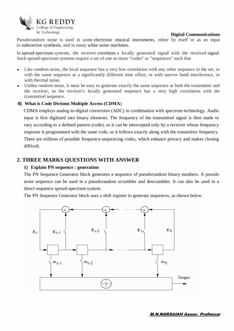
Digital CommunicationsPseudorandom noise is used in some electronic musical instruments, either by itself or as an input to subtractive synthesis, and in many white noise machines.
In spread-spectrum systems, the receiver correlates a locally generated signal with the received signal. Such spread-spectrum systems require a set of one or more "codes" or "sequences" such that
Like random noise, the local sequence has a very low correlation with any other sequence in the set, or with the same sequence at a significantly different time offset, or with narrow band interference, or with thermal noise.
Unlike random noise, it must be easy to generate exactly the same sequence at both the transmitter and the receiver, so the receiver's locally generated sequence has a very high correlation with the transmitted sequence.
4) What is Code Division Multiple Access (CDMA) CDMA employs analog-to-digital conversion (ADC) in combination with spectrum technology. Audio input is first digitized into binary elements. The frequency of the transmitted signal is then made to vary according to a defined pattern (code), so it can be intercepted only by a receiver whose frequency response is programmed with the same code, so it follows exactly along with the transmitter frequency. There are trillions of possible frequency-sequencing codes, which enhance privacy and makes cloning difficult.
2. THREE MARKS QUESTIONS WITH ANSWER
1) Explain PN sequence : generation The PN Sequence Generator block generates a sequence of pseudorandom binary numbers. A pseudo noise sequence can be used in a pseudorandom scrambler and descrambler. It can also be used in a direct-sequence spread-spectrum system. The PN Sequence Generator block uses a shift register to generate sequences, as shown below.

Digital CommunicationsAll r registers in the generator update their values at each time step according to the value of the incoming arrow to the shift register. The adders perform addition modulo 2. The shift register is described by the Generator Polynomial parameter, which is a primitive binary polynomial in z,
. The coefficient is 1 if there is a connection from
the kth register, as labeled in the preceding diagram, to the adder. The leading term and the
constant term of the Generator Polynomial parameter must be 1. You can specify the Generator polynomial parameter using either of these formats: A vector that lists the coefficients of the polynomial in descending order of powers. The first and last entries must be 1. Note that the length of this vector is one more than the degree of the generator polynomial. A vector containing the exponents of z for the nonzero terms of the polynomial in descending order of powers. The last entry must be 0.
For example, [1 0 0 0 0 0 1 0 1] and [8 2 0] represent the same polynomial, . The Initial states parameter is a vector specifying the initial values of the registers. The Initial states parameter must satisfy these criteria: All elements of the Initial states vector must be binary numbers. The length of the Initial states vector must equal the degree of the generator polynomial.
Note At least one element of the Initial states vector must be nonzero in order for the block to generate a nonzero sequence. That is, the initial state of at least one of the registers must be nonzero.
For example, the following table indicates two sets of parameter values that correspond to a generator
polynomial of .
Quantity Example 1 Example 2
Generator polynomial g1 = [1 0 0 0 0 0 1 0 1] g2 = [8 2 0]
Degree of generator polynomial 8, which is length(g1)-1 8
Initial states [1 0 0 0 0 0 1 0] [1 0 0 0 0 0 1 0]
The Shift parameter shifts the starting point of the output sequence. With the default setting for this parameter, the only connection is along the arrow labeled m0, which corresponds to a shift of 0. The parameter is described in greater detail below. You can shift the starting point of the PN sequence with the Shift parameter. You can specify the parameter in either of two ways:

Digital CommunicationsAn integer representing the length of the shift A binary vector, called the mask vector, whose length is equal to the degree of the generator polynomial The difference between the block's outputs when you set Shift (or mask) to 0, versus a positive integer d, is shown in the following table.
T = 0 T = 1 T = 2
T = d T = d+1
Shift = 0 x0 x1 x2
xd xd+1
Shift = d xd xd+1 xd+2
x2d x2d+1
Alternatively, you can set the Shift parameter to a binary vector, corresponding to a polynomial in z,
, of degree at most r - 1. The mask vector
corresponding to a shift of d is the vector that represents modulo g(z), where g(z) is the generator polynomial. For example, if the degree of the generator polynomial is 4, then the mask
vector corresponding to d = 2 is [0 1 0 0], which represents the polynomial . The preceding schematic diagram shows how the Shift (or mask) parameter is implemented when you specify it as a mask vector. The default setting for the Shift (or mask) parameter is [0 0 0 1], which corresponds to d = 0. You can calculate the mask vector using the Communications Toolbox function shift2mask. You can use an external signal to reset the values of the internal shift register to the initial state by selecting the Reset on nonzero input check box. This creates an input port for the external signal in the PN Sequence Generator block. The way the block resets the internal shift register depends on whether its output signal and the reset signal are sample-based or frame-based. The following example demonstrates the possible alternatives. 2) Explain Processing gain of SSM In a spread-spectrum system, the process gain (or "processing gain") is the ratio of the spread (or RF) bandwidth to the unspread (or baseband) bandwidth. It is usually expressed in decibels (dB). For example, if a 1 kHz signal is spread to 100 kHz, the process gain expressed as a numerical ratio would be 100000/1000 dB. Note that process gain does not reduce the effects of wideband thermal noise. It can be shown that a direct-sequence spread-spectrum (DSSS) system has exactly the same bit error behavior as a non-spread-spectrum system with the same modulation format. Thus, on an additive white Gaussian

Digital Communicationsnoise (AWGN) channel without interference, a spread system requires the same transmitter power as an unspread system, all other things being equal. Unlike a conventional communication system, however, a DSSS system does have a certain resistance against narrowband interference, as the interference is not subject to the process gain of the DSSS signal, and hence the signal-to-interference ratio is improved. In frequency modulation (FM), the processing gain can be expressed as
where: Gp is the processing gain, Bn is the noise bandwidth,
is the peak frequency deviation, W is the sinusoidal modulating frequency. 3) Draw model of spread spectrum digital communication system
4) Explain Code Division Multiple Access (CDMA) Code Division Multiple Access (CDMA) is a sort of multiplexing that facilitates various signals to occupy a single transmission channel. It optimizes the use of available bandwidth. The technology is commonly used in ultra-high-frequency (UHF) cellular telephone systems, bands ranging between the 800-MHz and 1.9-GHz. CDMA Overview

Digital CommunicationsCode Division Multiple Access system is very different from time and frequency multiplexing. In this system, a user has access to the whole bandwidth for the entire duration. The basic principle is that different CDMA codes are used to distinguish among the different users. Techniques generally used are direct sequence spread spectrum modulation (DS-CDMA), frequency hopping or mixed CDMA detection (JDCDMA). Here, a signal is generated which extends over a wide bandwidth. A code called spreading code is used to perform this action. Using a group of codes, which are orthogonal to each other, it is possible to select a signal with a given code in the presence of many other signals with different orthogonal codes. How Does CDMA Work? CDMA allows up to 61 concurrent users in a 1.2288 MHz channel by processing each voice packet with two PN codes. There are 64 Walsh codes available to differentiate between calls and theoretical limits. Operational limits and quality issues will reduce the maximum number of calls somewhat lower than this value. In fact, many different "signals" baseband with different spreading codes can be modulated on the same carrier to allow many different users to be supported. Using different orthogonal codes, interference between the signals is minimal. Conversely, when signals are received from several mobile stations, the base station is capable of isolating each as they have different orthogonal spreading codes. The following figure shows the technicality of the CDMA system. During the propagation, we mixed the signals of all users, but by that you use the same code as the code that was used at the time of sending the receiving side. You can take out only the signal of each user.
5) Define & Explain DSSS

Digital CommunicationsIn telecommunications, direct-sequence spread spectrum (DSSS) is a spread spectrum modulation technique used to reduce overall signal interference. The spreading of this signal makes the resulting wideband channel more noisy, allowing for greater resistance to unintentional and intentional interference. A method of achieving the spreading of a given signal is provided by the modulation scheme. With DSSS, the message signal is used to modulate a bit sequence known as a Pseudo Noise (PN) code; this PN code consists of a radio pulse that is much shorter in duration (larger bandwidth) than the original message signal. This modulation of the message signal scrambles and spreads the pieces of data, and thereby resulting in a bandwidth size nearly identical to that of the PN sequence.[1] In this context, the duration of the radio pulse for the PN code is referred to as the chip duration. The smaller this duration, the larger the bandwidth of the resulting DSSS signals; more bandwidth multiplexed to the message signal results in better resistance against interference.
3. FIVE MARKS QUESTIONS WITH ANSWER 1) Explain Direct sequence spread spectrum (DSSS) Bandwidth spreading by direct modulation of signals by a wideband spread signal (also called code) is called direct sequence spread spectrum (DS SS). The DSSS signal is then modulated by a carrier before final transmission. In DSSS, the base band signals are usually called bits, and the code bits are called chips. Typically, the baseband signal bandwidth is multiplies several times by the spreading signals. In other words, the chip rate is much higher than the bit rate. The spreading signal sequence is unique for a transmitter, and the same chip sequence is used at the receiver to re-construct the signals (data bits). A mechanism, by name correlation is used to synchronize the received spread signals (that contain data) with the locally generated code. At maximum received signal strength, correlation said to have occurred. The receiver then enters the tracking mode, such that the spread signal modulated signals are received without interruption. A simple DSSS system is described below: 1. DSSS Transmitter:
Where, d(t) is the input data bits c(t) is the code bits

Digital Communicationsx(t) is the frequency converted signal, ready for transmission. A note about why frequency up conversion is required for radio transmission: Base band, and very low frequencies are susceptible to heavy attenuation during transmission. In addition, imagine every transmitter transmitting in the base band frequencies. It is practically impossible for everyone to transmit in base band frequencies (A base band frequency is the frequency spectrum that is occupied by the unmodulated signals). Hence up-conversion of frequency is normally done to comply with the transmission requirements. In the DSSS transmitter, a code generator is a pseudo random generator that generates a known pseudo noise code sequence. Normally, the code has finite length (say 1024 chips), and repeats periodically. The requirements for a good PN code is discussed in a later section. An XOR gate can be used for spreading the data bits. The input, code, and the resulting output are displayed in the figure below:
In the figure shown above, each data bit is coded with 8 chips. In practice, this would be much higher, of the order of 1024 or even more. Higher the number of chips per bit, higher will be the processing gain. Processing gain is defined below: Processing Gain: One important parameter of DS SS receiver is the processing gain. Consider a data rate of 10KBPS, and Chip rate of 1MBPS. The processing gain is given by 10 log [rc/rb], where rc is the chip rate, and rb is the data rate. For a chip rate of 1MBPS, and a data rate of 1KBPS, the processing gain is 10log[1000] or 30dB. The processing gain is a measure of immunity to noise, and jamming signals. Higher the processing gain, more the band spread of the signals. Higher processing gain results in greater immunity to noise, and interfering signals. After spreading, the signals are unconverted and transmitted. 2. DSSS receiver: A simplified DS SS receiver block diagram is shown below.
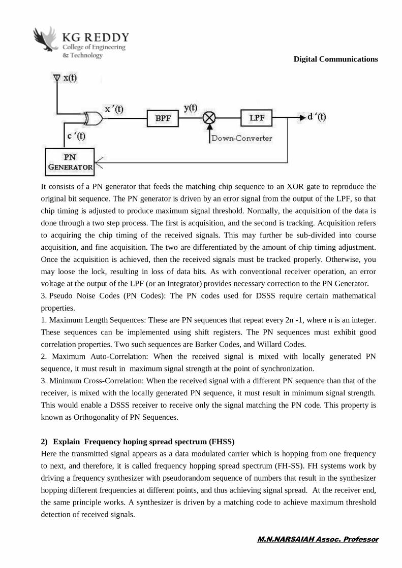
Digital Communications
It consists of a PN generator that feeds the matching chip sequence to an XOR gate to reproduce the original bit sequence. The PN generator is driven by an error signal from the output of the LPF, so that chip timing is adjusted to produce maximum signal threshold. Normally, the acquisition of the data is done through a two step process. The first is acquisition, and the second is tracking. Acquisition refers to acquiring the chip timing of the received signals. This may further be sub-divided into course acquisition, and fine acquisition. The two are differentiated by the amount of chip timing adjustment. Once the acquisition is achieved, then the received signals must be tracked properly. Otherwise, you may loose the lock, resulting in loss of data bits. As with conventional receiver operation, an error voltage at the output of the LPF (or an Integrator) provides necessary correction to the PN Generator. 3. Pseudo Noise Codes (PN Codes): The PN codes used for DSSS require certain mathematical properties. 1. Maximum Length Sequences: These are PN sequences that repeat every 2n -1, where n is an integer. These sequences can be implemented using shift registers. The PN sequences must exhibit good correlation properties. Two such sequences are Barker Codes, and Willard Codes. 2. Maximum Auto-Correlation: When the received signal is mixed with locally generated PN sequence, it must result in maximum signal strength at the point of synchronization. 3. Minimum Cross-Correlation: When the received signal with a different PN sequence than that of the receiver, is mixed with the locally generated PN sequence, it must result in minimum signal strength. This would enable a DSSS receiver to receive only the signal matching the PN code. This property is known as Orthogonality of PN Sequences. 2) Explain Frequency hoping spread spectrum (FHSS) Here the transmitted signal appears as a data modulated carrier which is hopping from one frequency to next, and therefore, it is called frequency hopping spread spectrum (FH-SS). FH systems work by driving a frequency synthesizer with pseudorandom sequence of numbers that result in the synthesizer hopping different frequencies at different points, and thus achieving signal spread. At the receiver end, the same principle works. A synthesizer is driven by a matching code to achieve maximum threshold detection of received signals.

Digital CommunicationsA simplified block schematic of a FH SS system is shown below: 1. FH-SS Transmitter: The transmitter consists of a baseband modulator followed by frequency synthesizer. The frequency synthesizer is driven by a PN generator. A PN generator may be built internal to the synthesizer.
2. FH-SS Receiver: A FH-SS receiver consists of a down converter followed by a demodulator. A synthesizer, driven by a matching PN generator is used to down convert the received signals. A maximum received signal threshold signifies locking.
c. Time Hopping (TH) SS Systems: Time hopping is not used as frequency as DSSS and FHSS. Time Hopping to spread the carrier is achieved by randomly spacing narrow transmitted pulses. The multiplicity factor is given by: Multiplicity factor = (average pulse spacing) / (pulse width). d. Recovery of Spread Spectrum Signals: Important Timing Signals In all cases of SS receivers, faithful recovery of the transmitted signals requires the following: a. Correlation Interval Synchronization: Receiving bits is achieved by proper correlator (or integrator) timing. Proper start/stop times for correlator are required for minimizing the received bit errors. b. SS Generator Synchronization: Timing signals are required to control the SS wave form generator signals. Direct Sequence systems employ a clock ticking at the chip rate 1/tc, and FH systems have a clock operating at the hopping rate.

Digital Communicationsc. Carrier Synchronization: Faithful reproduction of the transmitted signals to baseband requires down-conversion, and demodulation. This can be achieved only if the locally generated frequency and phase are in sync with the received carrier frequency. 3) Explain CDMA performance parameter and merits and demerits
CDMA Capacity
Processing Gain Signal to Noise Ratio Voice Activity Factor Frequency Reuse Efficiency
Capacity in CDMA is soft, CDMA has all users on each frequency and users are separated by code. This means, CDMA operates in the presence of noise and interference. In addition, neighboring cells use the same frequencies, which means no re-use. So, CDMA capacity calculations should be very simple. No code channel in a cell, multiplied by no cell. But it is not that simple. Although not available code channels are 64, it may not be possible to use a single time, since the CDMA frequency is the same.
Centralized Methods
The band used in CDMA is 824 MHz to 894 MHz (50 MHz + 20 MHz separation). Frequency channel is divided into code channels. 1.25 MHz of FDMA channel is divided into 64 code channels.
Processing Gain CDMA is a spread spectrum technique. Each data bit is spread by a code sequence. This means, energy per bit is also increased. This means that we get a gain of this. P (gain) = 10log (W/R) W is Spread Rate R is Data Rate For CDMA P (gain) = 10 log (1228800/9600) = 21dB This is a gain factor and the actual data propagation rate. On an average, a typical transmission condition requires a signal to the noise ratio of 7 dB for the adequate quality of voice. Translated into a ratio, signal must be five times stronger than noise. Actual processing gain = P (gain) - SNR = 21 7 = 14dB CDMA uses variable rate coder The Voice Activity Factor of 0.4 is considered = -4dB.

Digital CommunicationsHence, CDMA has 100% frequency reuse. Use of same frequency in surrounding cells causes some additional interference. In CDMA frequency, reuse efficiency is 0.67 (70% eff.) = -1.73dB
Advantages of CDMA CDMA has a soft capacity. The greater the number of codes, the more the number of users. It has the
CDMA requires a tight power control, as it suffers from near-far effect. In other words, a user near
the base station transmitting with the same power will drown the signal latter. All signals must have more or less equal power at the receiver
Rake receivers can be used to improve signal reception. Delayed versions of time (a chip or later) of the signal (multipath signals) can be collected and used to make decisions at the bit level.
Flexible transfer may be used. Mobile base stations can switch without changing operator. Two base stations receive mobile signal and the mobile receives signals from the two base stations.
Disadvantages of CDMA
The code length must be carefully selected. A large code length can induce delay or may cause interference.
Time synchronization is required. Gradual transfer increases the use of radio resources and may reduce capacity. As the sum of the power received and transmitted from a base station needs constant tight power
control. This can result in several handovers.

Digital Communications4) Explain the Use of spread spectrum
The SS Communications are widely used today for Military, Industrial, Avionics, Scientific, and Civil uses. The applications include the following:
1. Jam-resistant communication systems 2. CDMA radios: It is useful in multiple access communications wherein many users communicate
over a shared channel. Here the assignment of a unique spread spectrum sequence to each user allows him to simultaneously transmit over a common channel with minimal mutual interference. Such access technique often simplifies the network control requirements considerably.
3. High Resolution Ranging: SS Communications is often used in high resolution ranging. It is possible to locate an object with good accuracy using SS techniques. One example where it could be used is Global Positioning System (GPS). Here an object can use signals from several satellites transmitting SS signals according to a predefined format to determine its own position accurately on the globe.
4. WLAN: Wireless LAN (Local Area Networks) widely use spread spectrum communications. IEEE 802.11 is a standard that is developed for mobile communication, and widely implemented throughout the world. The standard defines three types of Physical Layer communications. These are:
a. Infrared (IR) Communications b. Direct Sequence Spread Spectrum Communications c. Frequency Hopping Spread Spectrum Communications.
Among the three, DSSS, and FHSS are widely used.
5. Cordless Phones: Several manufacturers implement Spread Spectrum in Cordless phones. The advantages of using spread spectrum in cordless phone include the following:
a. Security: Inherently, a ss communication is coded. b. Immunity to Noise: SS modulation is immune to noise when compared with other
modulation schemes such as AM and FM. c. Longer Range: Due to noise immunity, it is possible to achieve a longer range of
communications, for a very small transmitted power. 6. Long-range wireless phones for home and industry 7. Cellular base stations interconnection. 5) Explain the Comparison of DSSS & FHSS
FHSS vs DSSS

Digital CommunicationsSpread spectrum is a group of techniques that utilizes a much larger bandwidth in transmitting information than would otherwise occupy a fraction of the bandwidth used. This is done to achieve a certain effect. FHSS and DSSS, which stand for Frequency Hopping Spread Spectrum and Direct Sequence Spread Spectrum, are two spread spectrum techniques. The main difference is in how they spread the data into the wider bandwidth. FHSS utilizes frequency hopping while DSSS utilizes pseudo noise to modify the phase of the signal.
Frequency hopping is achieved by dividing the large bandwidth into smaller channels that would fit the data. The signal would then be sent pseudo-randomly into a different channel. Because only one of the channels is in use at any given time, you are actually wasting bandwidth equivalent to the data bandwidth multiplied by the number of channels minus one. DSSS spreads the information across the band in a very different manner. It does so by introducing pseudo-random noise into the signal to change its phase at any given time. This results in an output that closely resembles static noise and would appear as just that to
- be extracted from the noise as long as the pseudo-random sequence is known.
In order for the receiver to decode the transmitted information, it must be synchronized with the transmitter. For FHSS it is relatively easy as the transmitter simply waits on one of the channels and waits for a decodable transmission. Once it finds that out, it can then follow the sequence being used to follow the transmitter which jumps across the different channels. With DSSS, it is not as simple. A timing search algorithm needs to be employed for the receiver to correctly establish synchronization.

Digital Communications4.OBJECTIVE QUESTIONS WITH ANSWERS
1. Some advantages of spread spectrum are a) Low susceptibility b) Immunity to jamming c) Reduced interference d) All of the mentioned Answer: d Explanation: Advantages of spread spectrum are low susceptibility, reduced interference, immunity to jamming and co existence of multi path system. 2. Processing gain is the ratio of message bandwidth to signal bandwidth. a) True b) False Answer: b Explanation: Processing gain is the ratio of signal bandwidth to message bandwidth. 3. Which is better for avoiding jamming? a) Direct sequence spread spectrum b) Frequency hopping spread spectrum c) Time hopping spread spectrum d) None of the mentioned Answer: b Explanation: Frequency hopping spread spectrum is better for avoiding jamming. 4. Which is more bandwidth efficient? a) Direct sequence spread spectrum b) Frequency hopping spread spectrum c) Time hopping spread spectrum d) None of the mentioned Answer: c Explanation: Time hopping spread spectrum is more bandwidth efficient. 5. Which is simpler to implement? a) Direct sequence spread spectrum b) Frequency hopping spread spectrum c) Time hopping spread spectrum d) None of the mentioned

Digital CommunicationsAnswer: a Explanation: Direct sequence spread spectrum is more simpler to implement. 6. Which uses orthogonal codes? a) Synchronous CDMA b) Asynchronous CDMA c) Synchronous & Asynchronous CDMA d) None of the mentioned Answer: c Explanation: Synchronous CDMA uses orthogonal codes and asynchronous CDMA uses pseudorandom codes. 7. Which is more suitable when large number of transmitters is used? a) Synchronous CDMA b) Asynchronous CDMA c) Synchronous & Asynchronous CDMA d) None of the mentioned Answer: b Explanation: Asynchronous CDMA is more suitable for large number of transmitters. 8. CDMA rejects a) Narrow band interference b) Wide band interference c) Narrow & Wide band interference d) None of the mentioned Answer: a Explanation: CDMA effectively rejects narrow band interference. 9. Frequency planning is very essential in a) FDMA b) TDMA c) FDMA & TDMA d) None of the mentioned Answer: c Explanation: Frequency planning is necessary for both TDMA and FDMA. 10. CDMA uses a) Hard hand off b) Soft hand off c) Hard & Soft hand off d) None of the mentioned Answer: b Explanation: CDMA uses soft hand off which provides more reliable communication.

Digital Communications 5. FILL IN THE BLANK QUESTIONS WITH ANSWERS
1) ---------- techniques are methods by which a signal (e.g., an electrical, electromagnetic, or acoustic signal) generated with a particular bandwidth is deliberately spread in the frequency domain, resulting in a signal with a wider bandwidth.
2) Spread-spectrum telecommunications is a signal structuring technique that employs ----------, or a hybrid of these, which can be used for multiple access and/or multiple functions.
3) This makes it appear like --------. 4) The spread spectrum signal is used in -------. 5) --------- is defined as a coded sequence of 1s and 0s with certain auto-correlation properties. 6) -------- of a DS-SS system represents the gain achieved by processing a spread spectrum signal over
an unspread signal.
7) --------- is defined as ratio of average interference power J and the signal power Ps. 8) Depending on the rate of frequency hopping FHSS systems are classified into ---- and ------
frequency hopping. 9) In FHSS the ---------- is not greatly dependent on the distance. 10) In --------, more than one frequency hops are required to transmit one symbol.
Ans: 1) spread-spectrum 2) direct sequence, frequency hopping 3) Random noise 4) Jamming 5) A pseudo- noise (PN) sequence 6) The processing gain 7) Jamming margin 8) Slow and fast 9) Synchronization 10) Fast frequency hopping.

Digital Communications17. Beyond syllabus Topics with material
1) Additive White Gaussian Noise (AWGN)
The performance of a digital communication system is quantified by the probability of bit detection errors in the presence of thermal noise. In the context of wireless communications, the main source of thermal noise is addition of random signals arising from the vibration of atoms in the receiver electronics. It is called additive white Gaussian noise (AWGN) due to the following reasons: [Additive] The noise is additive, i.e., the received signal is equal to the transmitted signal plus noise. This gives the most widely used equality in communication systems, and is shown in Figure below. Remember that the below equation is highly simplified due to neglecting every single imperfection a Tx signal encounters, except the noise itself.
Moreover, this noise is statistically independent of the signal. [White] Just like the white color which is composed of all frequencies in the visible spectrum, white noise refers to the idea that it has uniform power across the whole frequency band. As a consequence, the spectral density of white noise is ideally flat for all frequencies ranging from to .

Digital Communications[Gaussian] The probability distribution of the noise samples is Gaussian, i.e., in time domain, the samples can acquire both positive and negative values and in addition, the values close to zero have a higher chance of occurrence while the values far away from zero are less likely to appear. This is shown in Figure below.
As a result, the time domain average of a large number of noise samples is zero. We will use this attribute over and over again throughout the system design.
Nyquist investigated the properties of thermal noise and showed that its power spectral density is equal to, where is a constant and is the temperature in Kelvin. As a consequence, the noise power is directly proportional to the equivalent temperature and hence the name thermal noise. Historically, this constant value indicated in noise spectral density Figure is denoted as Watts/Hz. When we view the constant spectral density as a rectangular sequence (we do not discuss random sequences here, so this discussion is just for a general understanding), its IDFT must be a unit impulse. Furthermore, in the article on correlation, we saw that the IDFT of the spectral density is the auto-correlation function of the signal. Combining these two facts, an implication of a constant spectral density is that the autocorrelation of the noise in time domain is a unit impulse, i.e., it is zero for all non-zero time shifts. In words, each noise sample in a sequence is uncorrelated with every other noise sample in the same sequence. In reality, the ideal flat spectrum from to is true for frequencies of interest in wireless communications (a few kHz to hundreds of GHz) but not for higher frequencies. Nevertheless, every wireless communication system involves filtering that removes most of the noise energy outside the spectral band occupied by our desired signal. Consequently after filtering, it is not possible to distinguish whether the spectrum was ideally flat or partially flat outside the band of interest. To help in mathematical analysis of the underlying waveforms resulting in closed-form expressions a holy grail of communication theory it can be assumed flat before filtering as shown in noise spectral density Figure. For a discrete signal with sampling rate, the sampling theorem dictates that the bandwidth is constrained by an above mentioned low pass filter within the range to avoid aliasing. This filter is an ideal low pass filter with the resulting in-band power is shown in red in Figure below, while the rest is filtered out.

Digital Communications
As with all densities, the value No is the amount of noise power Pw per unit bandwidth No=Pw/B Plugging B=Fs/2 in the above equation, the noise power in a sampled bandlimited system is given as Pw=No.Fs/2 Fooling the Randomness As we will see in our discussions about communication systems, a communication signal has a lot of structure in its construction. However, due to Gaussian nature of noise acquiring both positive and negative values, the result of adding a large number of noise-only samples tends to zero. Therefore, when a noisy signal is received, the Rx exploits this structure through correlating with what is expected. In the process, it estimates various unknown parameters and detects the actual message while averaging over a large number of observations. This correlation brings order out and averaging mitigates the harsh effects of noise. An AWGN channel is the most basic model of a communication system. Even simple practical systems suffer from various kinds of imperfections in addition to AWGN. Examples of systems operating largely in AWGN conditions are space communications with highly directional antennas and some point-to-point microwave links
2) Multiplexing In telecommunications and computer networks, multiplexing (sometimes contracted to muxing) is a method by which multiple analog or digital signals are combined into one signal over a shared medium. The aim is to share a scarce resource. For example, in telecommunications, several telephone calls may be carried using one wire. Multiplexing originated in telegraphy in the 1870s, and is now widely applied in communications. In telephony, George Owen Squire is credited with the development of telephone carrier multiplexing in 1910. The multiplexed signal is transmitted over a communication channel such as a cable. The multiplexing divides the capacity of the communication channel into several logical channels, one for each message signal or data stream to be transferred. A reverse process, known as demultiplexing, extracts the original channels on the receiver end. A device that performs the multiplexing is called a multiplexer (MUX), and a device that performs the reverse process is called a demultiplex (DEMUX or DMX).

Digital CommunicationsInverse multiplexing (IMUX) has the opposite aim as multiplexing, namely to break one data stream into several streams, transfer them simultaneously over several communication channels, and recreate the original data stream. Types :
Multiple variable bit rate digital bit streams may be transferred efficiently over a single mixed bandwidth channel by means of statistical multiplexing. This is an asynchronous mode time-domain multiplexing which is a form of time-division multiplexing. Digital bit streams can be transferred over an analog channel by means of code-division multiplexing techniques such as frequency-hopping spread spectrum (FHSS) and direct-sequence spread spectrum (DSSS).
In wireless communications, multiplexing can also be accomplished through alternating polarization (horizontal/vertical or clockwise/counterclockwise) on each adjacent channel and satellite, or through phased multi-antenna array combined with a multiple-input multiple-output communications (MIMO) scheme. Space-division multiplexing In wired communication, space-division multiplexing, also known as Space-division multiple access is the use of separate point-to-point electrical conductors for each transmitted channel. Examples include an analogue stereo audio cable, with one pair of wires for the left channel and another for the right channel, and a multi-pair telephone cable, a switched star network such as a telephone access network, a switched Ethernet network, and a mesh network.
In wireless communication, space-division multiplexing is achieved with multiple antenna elements forming a phased array antenna. Examples are multiple-input and multiple-output(MIMO), single-input and multiple-output (SIMO) and multiple-input and single-output (MISO) multiplexing. An IEEE 802.11n wireless router with k antennas makes it in principle possible to communicate with k multiplexed channels, each with a peak bit rate of 54 Mbit/s, thus increasing the total peak bit rate by the factor k. Different antennas would give different multi-path propagation (echo) signatures, making it possible for digital signal processing techniques to separate different signals from each other. These techniques may also be utilized for space diversity (improved robustness to fading) or beam forming (improved selectivity) rather than multiplexing Frequency-division multiplexing
Frequency-division multiplexing (FDM): The spectrum of each input signal is shifted to a distinct frequency range. Frequency-division multiplexing (FDM) is inherently an analog technology. FDM achieves the combining of several signals into one medium by sending signals in several distinct frequency ranges over a single medium. In FDM the signals are electrical signals. One of the most common applications for FDM is traditional radio and television broadcasting from terrestrial, mobile or satellite stations, or cable television.

Digital CommunicationsOnly one cable reaches a customer's residential area, but the service provider can send multiple television channels or signals simultaneously over that cable to all subscribers without interference. Receivers must tune to the appropriate frequency (channel) to access the desired signal. A variant technology, called wavelength-division multiplexing (WDM) is used in optical communications. Time-division multiplexing
Time-division multiplexing (TDM). Time-division multiplexing (TDM) is a digital (or in rare cases, analog) technology which uses time, instead of space or frequency, to separate the different data streams. TDM involves sequencing groups of a few bits or bytes from each individual input stream, one after the other, and in such a way that they can be associated with the appropriate receiver. If done sufficiently quickly, the receiving devices will not detect that some of the circuit time was used to serve another logical communication path. Consider an application requiring four terminals at an airport to reach a central computer. Each terminal communicated at 2400 baud, so rather than acquire four individual circuits to carry such a low-speed transmission; the airline has installed a pair of multiplexers. A pair of 9600 baud modems and one dedicated analog communications circuit from the airport ticket desk back to the airline data center are also installed.[1] Some web proxy servers (e.g. polipo) use TDM in HTTP pipelining of multiple HTTP transactions onto the same TCP/IP connection
Carrier sense multiple access and multi drop communication methods are similar to time-division multiplexing in that multiple data streams are separated by time on the same medium, but because the signals have separate origins instead of being combined into a single signal, are best viewed as channel access methods, rather than a form of multiplexing. Polarization-division multiplexing Polarization-division multiplexing uses the polarization of electromagnetic radiation to separate orthogonal channels. It is in practical use in both radio and optical communications, particularly in 100 Gbit/s per channel fiber optic transmission systems. Orbital angular momentum multiplexing Orbital angular momentum multiplexing is a relatively new and experimental technique for multiplexing multiple channels of signals carried using electromagnetic radiation over a single path.[3] It can potentially be used in addition to other physical multiplexing methods to greatly expand the transmission capacity of such systems. As of 2012 it is still in its early research phase, with small-scale laboratory demonstrations of bandwidths of up to 2.5 Tbit/s over a single light path.[4] This is a controversial subject in the academic community, with many claiming it is not a new method of multiplexing, but rather a special case of space-division multiplexing. Code-division multiplexing Code division multiplexing (CDM), Code division multiple access (CDMA) or spread spectrum is a class of techniques where several channels simultaneously share the same frequency spectrum, and this spectral

Digital Communicationsbandwidth is much higher than the bit rate or symbol rate. One form is frequency hopping; another is direct sequence spread spectrum. In the latter case, each channel transmits its bits as a coded channel-specific sequence of pulses called chips. Number of chips per bit, or chips per symbol, is the spreading factor. This coded transmission typically is accomplished by transmitting a unique time-dependent series of short pulses, which are placed within chip times within the larger bit time. All channels, each with a different code, can be transmitted on the same fiber or radio channel or other medium, and asynchronously demultiplexed. Advantages over conventional techniques are that variable bandwidth is possible (just as in statistical multiplexing), that the wide bandwidth allows poor signal-to-noise ratio according to Shannon-Hartley theorem, and that multi-path propagation in wireless communication can be combated by rake receivers.
A significant application of CDMA is the Global Positioning System (GPS).
Telecommunication multiplexing Multiple access method
A multiplexing technique may be further extended into a multiple access method or channel access method, for example, TDM into time-division multiple access (TDMA) and statistical multiplexing into carrier-sense multiple access (CSMA). A multiple access method makes it possible for several transmitters connected to the same physical medium to share its capacity.
Multiplexing is provided by the Physical Layer of the OSI model, while multiple access also involves a media access control protocol, which is part of the Data Link Layer.
The Transport layer in the OSI model, as well as TCP/IP model, provides statistical multiplexing of several application layer data flows to/from the same computer.
Code-division multiplexing (CDM) is a technique in which each channel transmits its bits as a coded channel-specific sequence of pulses. This coded transmission typically is accomplished by transmitting a unique time-dependent series of short pulses, which are placed within chip times within the larger bit time. All channels, each with a different code, can be transmitted on the same fiber and asynchronously demultiplexed. Other widely used multiple access techniques are time-division multiple access (TDMA) and frequency-division multiple access (FDMA). Code-division multiplex techniques are used as an access technology, namely code-division multiple access (CDMA), in Universal Mobile Telecommunications System (UMTS) standard for the third-generation (3G) mobile communication identified by the ITU.
Application areas Telegraphy The earliest communication technology using electrical wires, and therefore sharing an interest in the economies afforded by multiplexing, was the electric telegraph. Early experiments allowed two separate messages to travel in opposite directions simultaneously, first using an electric battery at both ends, then at only one end.

Digital Communications Émile Baudot developed a time-multiplexing system of multiple Hughes machines in the 1870s. In 1874, the quadruplex telegraph developed by Thomas Edison transmitted two messages in each
direction simultaneously, for a total of four messages transiting the same wire at the same time. Several workers were investigating acoustic telegraphy, a frequency-division multiplexing technique,
which led to the invention of the telephone. Telephony In telephony, a customer's telephone line now typically ends at the remote concentrator box, where it is multiplexed along with other telephone lines for that neighborhood or other similar area. The multiplexed signal is then carried to the central switching office on significantly fewer wires and for much further distances than a customer's line can practically go. This is likewise also true for digital subscriber lines (DSL). Fiber in the loop (FITL) is a common method of multiplexing, which uses optical fiber as the backbone. It not only connects POTS phone lines with the rest of the PSTN, but also replaces DSL by connecting directly to Ethernet wired into the home. Asynchronous Transfer Model is often the communications protocol used. Because all the phone (and data) lines have been clumped together, none of them can be accessed except through a demultiplexer. Where such demultiplexers are uncommon, this provides for more-secure communications, though the connections are not typically encrypted.
Cable TV has long carried multiplexed television channels, and late in the 20th century began offering the same services as telephone companies. IPTV also depends on multiplexing. Video processing Main article: Demultiplexer (media file)
In video editing and processing systems, multiplexing refers to the process of interleaving audio and video into one coherent data stream. In digital video, such a transport stream is normally a feature of a container format which may include metadata and other information, such as subtitles. The audio and video streams may have variable bit rate. Software that produces such a transport stream and/or container is commonly called a statistical multiplexer or muxer. A demuxer is software that extracts or otherwise makes available for separate processing the components of such a stream or container. Digital broadcasting In digital television and digital radio systems, several variable bit-rate data streams are multiplexed together to a fixed bit rate transport stream by means of statistical multiplexing. This makes it possible to transfer several video and audio channels simultaneously over the same frequency channel, together with various services. In the digital television systems, this may involve several standard definition television (SDTV) programmers (particularly on DVB-T, DVB-S2, ISDB and ATSC-C), or one HDTV, possibly with a single SDTV companion channel over one 6 to 8 MHz-wide TV channel. The device that accomplishes this is called a statistical multiplexer. In several of these systems, the multiplexing results in an MPEG transport stream. The newer DVB standards DVB-S2 and DVB-T2 have the capacity to carry several HDTV channels in one multiplex. Even the original DVB standards can carry more HDTV channels in a multiplex if the most advanced MPEG-4 compressions hardware is used.
On communications satellites which carry broadcast television networks and radio networks, this is known as multiple channels per carrier or MCPC. Where multiplexing is not practical (such as where there are different sources using a single transponder), single channel per carrier mode is used.

Digital CommunicationsSignal multiplexing of satellite TV and radio channels is typically carried out in a central signal playout and uplink centre, such as SES Platform Services in Germany, which provides playout, digital archiving, encryption, and satellite uplinks, as well as multiplexing, for hundreds of digital TV and radio channels.
In digital radio, both the Digital Audio Broadcasting (DAB) Eureka 147 system of digital audio broadcasting and the in-band on-channel HD Radio, FMeXtra, and Digital Radio Mondi ale systems can multiplex channels. This is essentially required with DAB-type transmissions (where a multiplex is called a DAB ensemble), but is entirely optional with IBOC systems. Analog broadcasting In FM broadcasting and other analog radio media, multiplexing is a term commonly given to the process of adding subcarriers to the audio signal before it enters the transmitter, where modulation occurs. (In fact, the stereo multiplex signal can be generated using time-division multiplexing, by switching between the two (left channel and right channel) input signals at an ultrasonic rate (the subcarrier), and then filtering out the higher harmonics.) Multiplexing in this sense is sometimes known as MPX, which in turn is also an old term for stereophonic FM, seen on stereo systems since the 1960s.

Digital Communications17. Topics beyond the syllabus with material OSI model
The Open Systems Interconnection model (OSI model) is a conceptual model that characterizes and standardizes the communication functions of a telecommunication or computing system without regard to its underlying internal structure and technology. Its goal is the interoperability of diverse communication systems with standard protocols. The model partitions a communication system into abstraction layer. The original version of the model defined seven layers. A layer serves the layer above it and is served by the layer below it. For example, a layer that provides error-free communications across a network provides the path needed by applications above it, while it calls the next lower layer to send and receive packets that comprise the contents of that path. Two instances at the same layer are visualized as connected by a horizontal connection in that layer. The model is a product of the Open Systems Interconnection project at the International Organization for Standardization (ISO), maintained by the identification ISO/IEC 7498-1.
Communication in the OSI-Model (example with layers 3 to 5)

Digital CommunicationsHistory In the late 1970s, one project was administered by the International Organization for Standardization (ISO), while another was undertaken by the International Telegraph and Telephone Consultative Committee (CCITT, from French: Comité Consultatif International Téléphonique et Télégraphique). These two international standards bodies each developed a document that defined similar networking models.
In 1983, these two documents were merged to form a standard called The Basic Reference Model for Open Systems Interconnection. The standard is usually referred to as the Open Systems Interconnection Reference Model, the OSI Reference Model, or simply the OSI model. It was published in 1984 by both the ISO, as standard ISO 7498, and the renamed CCITT (now called the Telecommunications Standardization Sector of the International Telecommunication Union or ITU-T) as standard X.200. OSI had two major components, an abstract model of networking, called the Basic Reference Model or seven-layer model, and a set of specific protocols. The concept of a seven-layer model was provided by the work of Charles Bachman at Honeywell Information Services. Various aspects of OSI design evolved from experiences with the ARPANET, NPLNET, EIN, CYCLADES network and the work in IFIP WG6.1. The new design was documented in ISO 7498 and its various addenda. In this model, a networking system was divided into layers. Within each layer, one or more entities implement its functionality. Each entity interacted directly only with the layer immediately beneath it, and provided facilities for use by the layer above it. Protocols enable an entity in one host to interact with a corresponding entity at the same layer in another host. Service definitions abstractly described the functionality provided to an (N)-layer by an (N-1) layer, where N was one of the seven layers of protocols operating in the local host. The OSI standards documents are available from the ITU-T as the X.200-series of recommendations.[1] Some of the protocol specifications were also available as part of the ITU-T X series. The equivalent ISO and ISO/IEC standards for the OSI model were available from ISO. Not all are free of charge.
Description of OSI layers The recommendation X.200 describes seven layers, labeled 1 to 7. Layer 1 is the lowest layer in this model.
OSI Model
Layer Protocol data unit (PDU) Function[3]
Host layers
7. Application
Data
High-level APIs, including resource sharing, remote file access
6. Presentation Translation of data between a networking service and an application; includingcharacter encoding, data compression and encryption/decryption
5. Session Managing communication sessions, i.e. continuous exchange of information in the form of multiple back-and-forth transmissions between two nodes
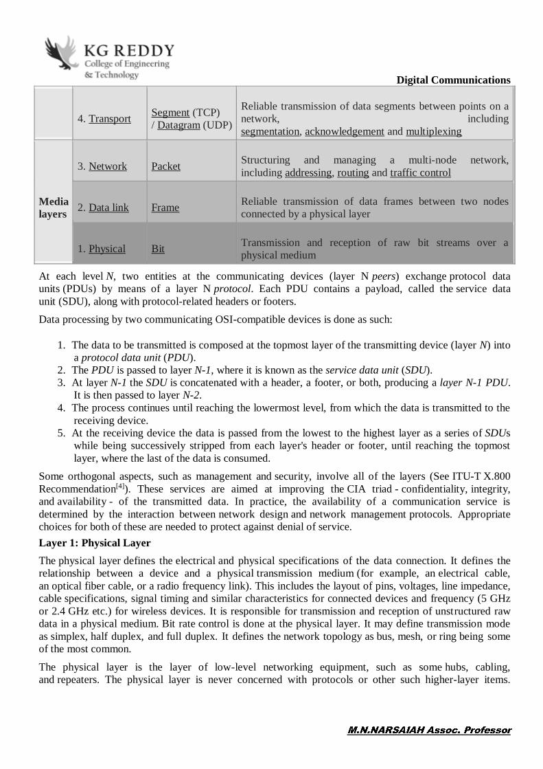
Digital Communications
4. Transport Segment (TCP) / Datagram (UDP)
Reliable transmission of data segments between points on a network, including segmentation, acknowledgement and multiplexing
Media layers
3. Network Packet
Structuring and managing a multi-node network, including addressing, routing and traffic control
2. Data link Frame
Reliable transmission of data frames between two nodes connected by a physical layer
1. Physical Bit
Transmission and reception of raw bit streams over a physical medium
At each level N, two entities at the communicating devices (layer N peers) exchange protocol data units (PDUs) by means of a layer N protocol. Each PDU contains a payload, called the service data unit (SDU), along with protocol-related headers or footers. Data processing by two communicating OSI-compatible devices is done as such:
1. The data to be transmitted is composed at the topmost layer of the transmitting device (layer N) into a protocol data unit (PDU).
2. The PDU is passed to layer N-1, where it is known as the service data unit (SDU). 3. At layer N-1 the SDU is concatenated with a header, a footer, or both, producing a layer N-1 PDU.
It is then passed to layer N-2. 4. The process continues until reaching the lowermost level, from which the data is transmitted to the
receiving device. 5. At the receiving device the data is passed from the lowest to the highest layer as a series of SDUs
while being successively stripped from each layer's header or footer, until reaching the topmost layer, where the last of the data is consumed.
Some orthogonal aspects, such as management and security, involve all of the layers (See ITU-T X.800 Recommendation[4]). These services are aimed at improving the CIA triad - confidentiality, integrity, and availability - of the transmitted data. In practice, the availability of a communication service is determined by the interaction between network design and network management protocols. Appropriate choices for both of these are needed to protect against denial of service. Layer 1: Physical Layer The physical layer defines the electrical and physical specifications of the data connection. It defines the relationship between a device and a physical transmission medium (for example, an electrical cable, an optical fiber cable, or a radio frequency link). This includes the layout of pins, voltages, line impedance, cable specifications, signal timing and similar characteristics for connected devices and frequency (5 GHz or 2.4 GHz etc.) for wireless devices. It is responsible for transmission and reception of unstructured raw data in a physical medium. Bit rate control is done at the physical layer. It may define transmission mode as simplex, half duplex, and full duplex. It defines the network topology as bus, mesh, or ring being some of the most common.
The physical layer is the layer of low-level networking equipment, such as some hubs, cabling, and repeaters. The physical layer is never concerned with protocols or other such higher-layer items.
Digital CommunicationsExamples of hardware in this layer are network adapters, repeaters, network hubs, modems, and fiber media converters. Layer 2: Data Link Layer The data link layer provides node-to-node data transfer a link between two directly connected nodes. It detects and possibly corrects errors that may occur in the physical layer. It defines the protocol to establish and terminate a connection between two physically connected devices. It also defines the protocol for flow control between them. IEEE 802 divides the data link layer into two sub layers:[5]
Medium access control (MAC) layer responsible for controlling how devices in a network gain access to a medium and permission to transmit data.
Logical link control (LLC) layer responsible for identifying and encapsulating network layer protocols, and controls error checking and frame synchronization.
The MAC and LLC layers of IEEE 802 networks such as 802.3 Ethernet, 802.11 Wi-Fi, and 802.15.4 ZigBee operate at the data link layer.
The Point-to-Point Protocol (PPP) is a data link layer protocol that can operate over several different physical layers, such as synchronous and asynchronous serial lines. The ITU-T G.hn standard, which provides high-speed local area networking over existing wires (power lines, phone lines and coaxial cables), includes a complete data link layer that provides both error correction and flow control by means of a selective-repeat sliding-window protocol. Layer 3: Network Layer The network layer provides the functional and procedural means of transferring variable length data sequences (called datagrams) from one node to another connected in "different networks". A network is a medium to which many nodes can be connected, on which every node has an address and which permits nodes connected to it to transfer messages to other nodes connected to it by merely providing the content of a message and the address of the destination node and letting the network find the way to deliver the message to the destination node, possibly routing it through intermediate nodes. If the message is too large to be transmitted from one node to another on the data link layer between those nodes, the network may implement message delivery by splitting the message into several fragments at one node, sending the fragments independently, and reassembling the fragments at another node. It may, but does not need to, report delivery errors.
Message delivery at the network layer is not necessarily guaranteed to be reliable; a network layer protocol may provide reliable message delivery, but it need not do so.
A number of layer-management protocols, a function defined in the management annex, ISO 7498/4, belong to the network layer. These include routing protocols, multicast group management, network-layer information and error, and network-layer address assignment. It is the function of the payload that makes these belong to the network layer, not the protocol that carries them.[6] Layer 4: Transport Layer The transport layer provides the functional and procedural means of transferring variable-length data sequences from a source to a destination host via one or more networks, while maintaining the quality of service functions.
An example of a transport-layer protocol in the standard Internet stack is Transmission Control Protocol (TCP), usually built on top of the Internet Protocol (IP).
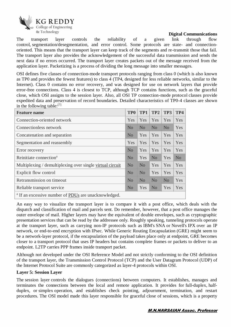
Digital CommunicationsThe transport layer controls the reliability of a given link through flow control, segmentation/desegmentation, and error control. Some protocols are state- and connection-oriented. This means that the transport layer can keep track of the segments and re-transmit those that fail. The transport layer also provides the acknowledgement of the successful data transmission and sends the next data if no errors occurred. The transport layer creates packets out of the message received from the application layer. Packetizing is a process of dividing the long message into smaller messages.
OSI defines five classes of connection-mode transport protocols ranging from class 0 (which is also known as TP0 and provides the fewest features) to class 4 (TP4, designed for less reliable networks, similar to the Internet). Class 0 contains no error recovery, and was designed for use on network layers that provide error-free connections. Class 4 is closest to TCP, although TCP contains functions, such as the graceful close, which OSI assigns to the session layer. Also, all OSI TP connection-mode protocol classes provide expedited data and preservation of record boundaries. Detailed characteristics of TP0-4 classes are shown in the following table:[7] Feature name TP0 TP1 TP2 TP3 TP4 Connection-oriented network Yes Yes Yes Yes Yes Connectionless network No No No No Yes Concatenation and separation No Yes Yes Yes Yes Segmentation and reassembly Yes Yes Yes Yes Yes Error recovery No Yes Yes Yes Yes Reinitiate connectiona No Yes No Yes No Multiplexing / demultiplexing over single virtual circuit No No Yes Yes Yes Explicit flow control No No Yes Yes Yes Retransmission on timeout No No No No Yes Reliable transport service No Yes No Yes Yes a If an excessive number of PDUs are unacknowledged.
An easy way to visualize the transport layer is to compare it with a post office, which deals with the dispatch and classification of mail and parcels sent. Do remember, however, that a post office manages the outer envelope of mail. Higher layers may have the equivalent of double envelopes, such as cryptographic presentation services that can be read by the addressee only. Roughly speaking, tunneling protocols operate at the transport layer, such as carrying non-IP protocols such as IBM's SNA or Novell's IPX over an IP network, or end-to-end encryption with IPsec. While Generic Routing Encapsulation (GRE) might seem to be a network-layer protocol, if the encapsulation of the payload takes place only at endpoint, GRE becomes closer to a transport protocol that uses IP headers but contains complete frames or packets to deliver to an endpoint. L2TP carries PPP frames inside transport packet. Although not developed under the OSI Reference Model and not strictly conforming to the OSI definition of the transport layer, the Transmission Control Protocol (TCP) and the User Datagram Protocol (UDP) of the Internet Protocol Suite are commonly categorized as layer-4 protocols within OSI. Layer 5: Session Layer The session layer controls the dialogues (connections) between computers. It establishes, manages and terminates the connections between the local and remote application. It provides for full-duplex, half-duplex, or simplex operation, and establishes check pointing, adjournment, termination, and restart procedures. The OSI model made this layer responsible for graceful close of sessions, which is a property

Digital Communicationsof the Transmission Control Protocol, and also for session check pointing and recovery, which is not usually used in the Internet Protocol Suite. The session layer is commonly implemented explicitly in application environments that use remote procedure calls. Layer 6: Presentation Layer The presentation layer establishes context between application-layer entities, in which the application-layer entities may use different syntax and semantics if the presentation service provides a mapping between them. If a mapping is available, presentation service data units are encapsulated into session protocol data units and passed down the protocol stack.
This layer provides independence from data representation by translating between application and network formats. The presentation layer transforms data into the form that the application accepts. This layer formats data to be sent across a network. It is sometimes called the syntax layer.[8] The presentation layer can include compression functions.[9] The Presentation Layer negotiates the Transfer Syntax.
The original presentation structure used the Basic Encoding Rules of Abstract Syntax Notation One (ASN.1), with capabilities such as converting an EBCDIC-coded text file to an ASCII-coded file, or serialization of objects and other data structures from and to XML. ASN.1 effectively makes an application protocol invariant with respect to syntax. Layer 7: Application Layer The application layer is the OSI layer closest to the end user, which means both the OSI application layer and the user interact directly with the software application. This layer interacts with software applications that implement a communicating component. Such application programs fall outside the scope of the OSI model. Application-layer functions typically include identifying communication partners, determining resource availability, and synchronizing communication. When identifying communication partners, the application layer determines the identity and availability of communication partners for an application with data to transmit. The most important distinction in the application layer is the distinction between the application-entity and the application. For example, a reservation website might have two application-entities: one using HTTP to communicate with its users, and one for a remote database protocol to record reservations. Neither of these protocols have anything to do with reservations. That logic is in the application itself. The application layer per se has no means to determine the availability of resources in the network.
Cross-layer functions
Cross-layer functions are services that are not tied to a given layer, but may affect more than one layer. Examples include the following:
Security service (telecommunication)[4] as defined by ITU-T X.800 recommendation. Management functions, i.e. functions that permit to configure, instantiate, monitor, terminate the
communications of two or more entities: there is a specific application-layer protocol, common management information protocol (CMIP) and its corresponding service, common management information service (CMIS), they need to interact with every layer in order to deal with their instances.
Multiprotocol Label Switching (MPLS) MPLS, ATM, and X.25 are 3a protocols. OSI divides the Network Layer into 3 roles: 3a) Subnetwork Access, 3b) Subnetwork Dependent Convergence and 3c) Subnetwork Independent Convergence. It was designed to provide a unified data-carrying service for both circuit-based clients and packet-switching clients which provide a datagram-based service model. It can be used to carry many different kinds of traffic, including IP packets, as well as native ATM, SONET, and Ethernet frames. Sometimes one sees reference to a Layer 2.5. This is a fiction create by

Digital Communicationsthose who are unfamiliar with the OSI Model and ISO 8648, Internal Organization of the Network Layer in particular.
ARP determines the mapping of an IPv4 address to the underlying MAC address. This is not a translation function. If it were IPv4 and the MAC address would be at the same layer. The implementation of the MAC protocol decodes the MAC PDU and delivers the User-Data to the IP-layer. Because Ethernet is a multi-access media, a device sending a PDU on an Ethernet segment needs to know what IP address maps to what MAC address.
DHCP, DHCP assigns IPv4 addresses to new systems joining a network. There is no means to derive or obtain an IPv4 address from an Ethernet address.
Domain Name Service is an Application Layer service which is used to look up the IP address of a given domain name. Once a reply is received from the DNS server, it is then possible to form a Layer 4 connection or flow to the desired host. There are no connections at Layer 3.
Cross MAC and PHY Scheduling is essential in wireless networks because of the time varying nature of wireless channels. By scheduling packet transmission only in favorable channel conditions, which requires the MAC layer to obtain channel state information from the PHY layer, network throughput can be significantly improved and energy waste can be avoided.
Interfaces: Neither the OSI Reference Model nor OSI protocols specify any programming interfaces, other than deliberately abstract service specifications. Protocol specifications precisely define the interfaces between different computers, but the software interfaces inside computers, known as network sockets are implementation-specific. For example, Microsoft Windows' Winsock, and Unix's Berkeley sockets and System V Transport Layer Interface, are interfaces between applications (layer 5 and above) and the transport (layer 4). NDIS and ODI are interfaces between the media (layer 2) and the network protocol (layer 3).
Interface standards, except for the physical layer to media, are approximate implementations of OSI service specifications.

Digital Communications
Introduction to Fading
About Fading
A transmitted signal undergoes changes while traveling through the propagation path to the receiver. The effect of these changes is commonly called fading. In free-space, a signal follows one path and arrives at the receiver with little attenuation. This is not the case for a signal that encounters obstacles in the propagation path. Instead, the signal is reflected, diffracted, and scattered from objects that are present in the path. Each path can have a different amount of attenuation, delay, and fading type. The combination of these different paths is termed multipath fading or multipath propagation. Simulating different numbers of paths with different fading configurations is essential for thoroughly testing receiver performance. At the receiver, the signals can add constructively or destructively, causing random and rapid fluctuations in the received amplitude when the receiver or the transmitter is moving. Due to the Doppler effect, this situation also causes the signal to be spread in the frequency domain. The fading phenomena can be classified into two main groups known as large scale fading and small scale fading. The large scale fading is used to describe the signal level at the receiver after traveling over a large area (hundreds of wavelengths). Small scale fading is used to describe the signal level at the receiver after encountering obstacles near (several wavelengths to fractions of wavelengths) the receiver.
Large-scale fading is the result of signal attenuation due to signal propagation over large distances and diffraction around large objects in the propagation path. Relative Path Loss (loss due to distance) In free-space, the attenuation of a signal due to distance follows the 1/d2 law, where d is the distance between the transmitter and the receiver. This is the case for line-of-sight (LOS) signals (path B). In the case of non-line-of-sight (NLOS) signals (path A), the attenuation is more likely to be anywhere from 1/d3 to 1/d6. This additional loss of power in propagation channels occurs when part of the reflected signal is lost. Shadowing Log normal shadowing is the result of the signal being blocked by large objects in the propagation path (path D). These are typically distant objects in the environment such as mountains, hills, or large buildings. The length of time it takes for a moving receiver to pass through the "shadow" of these obstacles brings about the term "slow fading". The statistical model used to describe shadowing is the log-normal distribution of the mean signal power.
Rayleigh Fading

Digital CommunicationsRayleigh fading is used to simulate the rapid amplitude fluctuations where there is no direct ray component. Because there is no direct ray component, Rayleigh fading is often classified as the worst case fading type. Using a one ray model, this small scale distribution simulates the effects of rapid amplitude fluctuations when the receiver travels a distance of a few wavelengths. The one ray is scattered near the receiver resulting in a large number of rays arriving at the receiver from all directions (path C). The signals add in and out of phase giving rise to amplitude fluctuations that vary at a rate that is dependent on the speed of the receiver. The statistical model used to describe the amplitude variations is the Rayleigh probability distribution function. The receiver movement also produces a spreading of the signal in the frequency domain due to the Doppler effect.
Rician Fading The Rician model adds a line-of-sight component to the Rayleigh model. The angle of arrival of the LOS component can be adjusted. In effect, this adds a bias to the Rayleigh probability distribution function. The ratio of signal power in the LOS component to the (local-mean) scattered power of the Rayleigh modulated component is defined as the K-factor. This model is often used to simulate a rural environment. Suzuki Fading Suzuki fading superimposes the log normal distribution onto the Rayleigh distribution. This is often used to simulate the effects of a dense urban environment with the average received power level fluctuating slowly due to shadowing effects. The log normal distribution is defined by the standard deviation of the average signal power level and a decorrelation length, which determines the rate at which the average power level changes. The decorrelation length determines the size of the shadow the receiver is moving through. The decorrelation length along with the vehicle speed determines the actual rate at which the average signal power level changes at the receiver. The following equation relates the decorrelation length to the log normal fading rate:
Pure Doppler Doppler shift is the frequency shift of the signal due to the relative motion between the transmitter and receiver. The frequency shift is calculated based on the speed of the mobile, the direction of motion and the angle of arrival of the signal. This applies to the direct ray case (no local reflectors).
MIMO technologies hold the promise of higher data rates and increased spectral efficiency by taking advantage of the richness of a multipath environment. Ideally, MIMO systems provide dramatic channel capacity gain through increased spatial diversity. However, this capacity is greatly reduced if the fading characteristic among various channels is correlated.
Digital CommunicationsSpatial Correlation Traditional methods for modeling wireless channels, such as Power Delay Profile and Doppler spectrum can accurately represent the multipath effects is a single-input, single-output (SISO) system. However, they do not typically include the spatial characteristics that may introduce correlation between the channels of a MIMO system. These spatial effects include: the power azimuth spectrum, antenna position and polarization within the multipath environment, and the gain pattern of the individual antenna elements. As MIMO operation requires low channel-to-channel correlation, it is important to understand how the contribution of each of these spatial characteristics may affect system performance. Spatial Characteristics The power azimuth spectrum characterizes the angle spread associated with angles that may be different for the signal paths connecting transmit/receive antenna pairs. Systems operating with a narrow range of angular spread may require antennas physically placed far apart in order to achieve low spatial correlation. In applications where antenna spacing is limited, "cross" polarized antennas coupled with antenna spacing, may help reduce the spatial correlation. Additionally, selecting the antenna pattern of the individual antenna elements, such as omni-directional or directive, can provide an optimal gain pattern for the antenna array depending on the multipath environment.