united nations - wltp.readthedocs.io€¦ · web view(a)type of internal combustion engine: fuel...
TRANSCRIPT

Economic Commission for EuropeInland Transport Committee World Forum for Harmonization of Vehicle Regulations
Working Party on Pollution and Energy
Sixty-seventh session Geneva, 14 November 2013 Item 2 of the provisional agendaWorldwide harmonized Light vehicles Test Procedures (WLTP)
Proposal for a new UN Global Technical Regulation on Worldwide harmonized Light vehicles Test Procedures (WLTP)
Submitted by the experts from the European Commission and Japan*, ****
The text reproduced below was prepared by the experts from the European Commission and Japan, building on the work of the informal working group on Worldwide harmonized Light vehicles Test Procedures (WLTP) and its sub-groups. It follows the proposal to develop a new global technical regulation on worldwide harmonized light vehicle test procedures (ECE/TRANS/WP.29/AC.3/26 and 26/Add.1).
* * In accordance with the programme of work of the Inland Transport Committee for 2010–2014 (ECE/TRANS/208, para. 106 and ECE/TRANS/2010/8, programme activity 02.4), the World Forum will develop, harmonize and update Regulations in order to enhance the performance of vehicles. The present document is submitted in conformity with that mandate.
** ** This document was submitted late due to its complexity, due to late inputs from other sources, and in order to include the information on the latest progress on this work.
GE.
United Nations ECE/TRANS/WP.29/GRPE/2013/13
Economic and Social Council Distr.: General17 September 2013
Original: English

ECE/TRANS/WP.29/GRPE/2013/13
Draft UN Global Technical Regulation on Worldwide harmonized Light vehicle Test Procedures (WLTP)
I. Statement of technical rationale and justification
A. Introduction
1. The compliance with emission standards is a central issue of vehicle certification worldwide. Emissions comprise criteria pollutants having a direct (mainly local) negative impact on health and environment, as well as pollutants having a negative environmental impact on a global scale. Regulatory emission standards typically are complex documents, describing measurement procedures under a variety of well-defined conditions, setting limit values for emissions, but also defining other elements such as the durability and on-board monitoring of emission control devices.
2. Most manufacturers produce vehicles for a global clientele or at least for several regions. Albeit vehicles are not identical worldwide since vehicle types and models tend to cater to local tastes and living conditions, the compliance with different emission standards in each region creates high burdens from an administrative and vehicle design point of view. Vehicle manufacturers therefore have a strong interest in harmonising vehicle emission test procedures and performance requirements as much as possible on a global scale. Regulators also have an interest in global harmonization since it offers more efficient development and adaptation to technical progress, potential collaboration at market surveillance and facilitates the exchange of information between authorities.
3. As a consequence stakeholders launched the work for this UN Global Technical Regulation (GTR) on worldwide harmonized light vehicle test procedures (WLTP) that aims at harmonising emission related test procedures for light duty vehicles to the extent this is possible. Vehicle test procedures need to represent real driving conditions as much as possible to make the performance of vehicles at certification and in real life comparable. Unfortunately, this aspect puts some limitations on the level of harmonization to be achieved, since for instance, ambient temperatures vary widely on a global scale. In addition, due to the different levels of development, different population densities and the costs associated with emission control technology, the regulatory stringency of legislation is expected to be different from region to region for the foreseeable future. Therefore, for instance, the setting of emission limit values is not part of this GTR for the time being.
4. The purpose of a GTR is its implementation into regional legislation by as many Contracting Parties as possible. However, the scope of regional legislations in terms of vehicle categories concerned depends on regional conditions and cannot be predicted for the time being. On the other hand, according to the rules of the 1998 UNECE agreement, Contracting Parties implementing a GTR must include all equipment falling into the formal GTR scope. Care must be taken, so that an unduly large formal scope of the GTR does not prevent its regional implementation. Therefore the formal scope of this GTR is kept to the core of light duty vehicles. However, this limitation of the formal GTR scope does not indicate that it could not be applied to a larger group of vehicle categories by regional legislation. In fact, Contracting Parties are encouraged to extend the scope of regional implementations of this GTR if this is technically, economically and administratively appropriate.
5. This first version of the WLTP GTR, in particular, does not contain any specific test requirements for dual fuel vehicles and hybrid vehicles not based on a combination of an
2

ECE/TRANS/WP.29/GRPE/2013/13
internal combustion engine and an electric machine. For example, specific requirements for hybrids using fuel cells or compressed gases as energy storage are not covered. Therefore these vehicles are not included in the scope of the WLTP GTR. Contracting Parties may however apply the WLTP GTR provisions to such vehicles to the extent it is possible and complement them by additional provisions, e.g. emission testing with different fuel grades and types, in regional legislation.
B. Procedural background and future development of the WLTP
6. In its November 2007 session, WP.29 decided to set up an informal WLTP group under GRPE to prepare a roadmap for the development of the WLTP. After various meetings and intense discussions, WLTP presented in June 2009 a first road map consisting of 3 phases, which was subsequently revised a number of times and contains the following main tasks:
(a) Phase 1 (2009 – 2014): development of the worldwide harmonised light duty driving cycle and associated test procedure for the common measurement of criteria compounds, CO2, fuel and energy consumption.
(b) Phase 2 (2014 – 2018): low temperature/high altitude test procedure, durability, in-service conformity, technical requirements for on-board diagnostics (OBD), mobile air-conditioning (MAC) system energy efficiency, off-cycle/real driving emissions.
(c) Phase 3 (2018 - …): emission limit values and OBD threshold limits, definition of reference fuels, comparison with regional requirements.
7. It should be noted that since the beginning of the WLTP process the European Union had a strong political objective set by its own legislation (Regulations (EC) 443/2009 and 510/2011) to implement a new and more realistic test cycle by 2014, which was a major political driving factor for setting the time frame of phase 1.
8. For the work of phase 1 the following working groups and sub-groups were established:
(a) Development of harmonised cycle (DHC): construction of a new Worldwide Light-duty Test Cycle (WLTC), i.e. the driving curve of the WLTP, based on the statistical analysis of real driving data.
The DHC group started working in September 2009, launched the collection of driving data in 2010 and proposed a first version of the driving cycle by mid-2011, which was revised a number of times to take into consideration technical issues such as driveability and better representativeness of driving conditions after a first validation.
(b) Development of test procedures (DTP): development of test procedures with the following specific expert groups,
(i) PM-PN: Particle mass (PM) and particle number (PN) measurements.
(ii) APM: Additional pollutant measurements, i.e. measurement procedures for exhaust substances which are not regulated yet
as compounds but may be regulated in the near future, such as NO2, ethanol, aldehydes, and ammonia.
(iii) LabProcICE: test conditions and measurement procedures of existing regulated compounds for vehicles equipped with internal combustion engines (other than PM and PN).
3

ECE/TRANS/WP.29/GRPE/2013/13
(iv) EV-HEV: specific test conditions and measurement procedures for electric and hybrid-electric vehicles.
(v) REF-FUEL: definition of reference fuels.
The DTP group started working in April 2010.
9. This first version of the GTR will only contain results of phase 1. During the work of the DTP group it became clear that a number of issues, in particular but not only in relation to electric and hybrid-electric vehicles, could not be resolved in time for an adoption of the first version of the WLTP GTR by WP.29 in March 2014. Therefore it was agreed that these elements would be further developed by the existing expert groups and should be adopted as a "phase 1b" amendment to the WLTP GTR within an appropriate time frame. Without claiming completeness "phase 1b" should address the following work items:
(a) LabProcICE:
(i) normalization methods, drive trace index;
(ii) energy economy rating and absolute speed change rating for speed trace violations;
(iii) wind tunnel as alternative method for road load determination;
(iv) supplemental test with representative regional temperature and soak period.
(b) EV-HEV:
(i) calculation method of each phase range for pure electric vehicles (PEVs);
(ii) shortened test procedure for PEV range test;
(iii) combined CO2 (fuel consumption) of each phase for off-vehicle charging hybrid electric vehicles (OVC-HEVs);
(iv) hybrid Electric Vehicle (HEV)/PEV power and maximum speed;
(v) combined test approach for OVC-HEVs and PEVs;
(vi) fuel cell vehicles;
(vii) utility factors;
(viii) preconditioning;
(ix) predominant mode.
(c) APM:
measurement method for ammonia, ethanol and aldehydes.
(d) DHC:
(i) speed violation criteria;
(ii) further downscaling in wide open throttle (WOT) operation;
(iii) sailing and gear shifting.
4

ECE/TRANS/WP.29/GRPE/2013/13
C. Background on driving cycles and test procedures
10. The development of the worldwide harmonised light duty vehicle driving cycle was based on experience gained from work on the world-wide heavy-duty certification procedure (WHDC), world-wide motorcycle test cycle (WMTC) and other national cycles.
11. The WLTC is a transient cycle by design. For constructing the WLTC, driving data from all participating Contracting Parties were collected and weighted according to the relative contribution of regions to the globally driven mileage and data collected for WLTP purpose.
12. The resulting driving data were subsequently cut into idling periods and "short trips" (i.e. driving events between two idling periods). By randomised combinations of these segments, a large number of "draft cycles" were generated. From the latter "draft cycle" family, the cycle best fitting certain dynamic properties of the original WLTP database was selected as a first "raw WLTC". In the subsequent work the "raw WLTC" was further processed, in particular with respect to its driveability and better representativeness, to obtain the final WLTC.
13. The driveability of the WLTC was assessed extensively during the development process and is supported by three distinct validation phases. Specific cycle versions for certain vehicles with limited driving capabilities due to a low power/mass ratio or limited maximum vehicle speed have been introduced. In addition, the drive trace to be followed by a test vehicle will be downscaled according to a mathematically prescribed method if the vehicle would have to encounter an unduly high proportion of "full throttle" driving in order to follow the original drive trace . Gear shift points are determined according to a mathematical procedure that is based on the characteristics of individual vehicles, what also enhances the driveability of the WLTC.
14. For the development of the test procedures, the DTP sub-group took into account existing emissions and energy consumption legislation, in particular those of the 1958 and 1998 Agreements, those of Japan and the United States Environmental Protection Agency (US EPA) Standard Part 1066. These test procedures were critically reviewed, compared to each other, updated to technical progress and complemented by new elements where necessary.
D. Technical feasibility, anticipated costs and benefits
15. At the design and validation of the WLTP strong emphasis has been put on its practicability, which is ensured by a number of measures explained above.
16. While in general the WLTP has been defined on the basis of the best technology available at the moment of its drafting, the practical facilitation of the WLTP procedures on a global scale has been kept in mind as well. The latter had some impact e.g. on the definition of set values and tolerances for several test parameters, such as the test temperature or deviations from the drive trace . Also, facilities without the most recent technical equipment should be able to perform WLTP certifications, leading to higher tolerances than those which would have been required just by best performing facilities.
17. The replacement of a regional test cycle by the WLTP initially will bear some costs for vehicle manufacturers, technical services and authorities, at least considered on a local scale, since some test equipment and procedures have to be upgraded. However, these costs should be limited since such upgrades are done regularly as adaptations to the technical progress. Related costs would have to be quantified on a regional level since they largely depend on the local conditions.
5

ECE/TRANS/WP.29/GRPE/2013/13
18. As pointed out in the technical rationale and justification, the principle of a globally harmonised light duty vehicle test procedure offers potential cost reductions for vehicle manufacturers. The design of vehicles can be better unified on a global scale and administrative procedures may be simplified. The monetary quantification of these benefits depends largely on the extent and timing of implementations of the WLTP in regional legislation.
19. The WLTP provides a higher representation of real driving conditions when compared to the previous regional driving cycles. Therefore, benefits are expected from the resulting consumer information about fuel and energy consumption. In addition the more representative WLTP will set proper incentives for implementing those CO 2 saving vehicle technologies that are also the most effective in real driving. The effectiveness of technology cost relative to the real driving CO2 saving will therefore be improved with respect to existing less representative driving cycles.
6

ECE/TRANS/WP.29/GRPE/2013/13
II. Text of the Global Technical Regulation
1. Purpose
This Global Technical Regulation (GTR) aims at providing a worldwide harmonised method to determine the levels of gaseous, particulate matter, particle number and CO2 emissions, fuel consumption, electric energy consumption and electric range from light-duty vehicles in a repeatable and reproducible manner designed to be representative of real world vehicle operation. The results will provide the basis for the regulation of these vehicles within regional type approval and certification procedures.
2. Scope and application
This GTR applies to vehicles of categories 1-2 and 2, both having a technically permissible maximum laden not exceeding 3,500 kg, and to all vehicles of category 1-1.
3. Definitions
3.1. Test equipment
3.1.1. "Accuracy" means the difference between a measured value and a reference value, traceable to a national standard and describes the correctness of a result. See Figure 1.
3.1.2. "Calibration" means the process of setting a measurement system's response so that its output agrees with a range of reference signals. Contrast with "verification".
3.1.3. "Calibration gas" means a gas mixture used to calibrate gas analysers.
3.1.4. "Double dilution method" means the process of separating a part of the diluted exhaust flow and mixing it with an appropriate amount of dilution air prior to the particulate sampling filter.
3.1.5. "Full-flow exhaust dilution system" means the continuous dilution of the total vehicle exhaust with ambient air in a controlled manner using a constant volume sampler (CVS).
3.1.6. "Linearization" means the application of a range of concentrations or materials to establish a mathematical relationship between concentration and system response.
3.1.7. "Non-methane hydrocarbons" (NMHC) is the total hydrocarbons (THC) minus the methane (CH4) contribution.
3.1.8. "Precision" means the degree to which repeated measurements under unchanged conditions show the same results (Figure 1). In this GTR, precision requirements always refer to one standard deviation.
3.1.9. "Reference value" means a value traceable to a national standard. See Figure 1.
7

value
precision
accuracy
reference value
probability density
ECE/TRANS/WP.29/GRPE/2013/13
3.1.10. "Set point" means the target value a control system aims to reach.
3.1.11. "Span" means to adjust an instrument so that it gives a proper response to a calibration standard that represents between 75 per cent and 100 per cent of the maximum value in the instrument range or expected range of use.
3.1.12. "Total hydrocarbons" (THC) means all volatile compounds measurable by a flame ionization detector (FID).
3.1.13. "Verification" means to evaluate whether or not a measurement system's output agrees with applied reference signals within one or more predetermined thresholds for acceptance.
3.1.14. "Zero gas" means a gas containing no analyte, which is used to set a zero response on an analyser.
Figure 1Definition of accuracy, precision and reference value
3.2. Road and dynamometer load
3.2.1. "Aerodynamic drag" means the force that opposes a vehicle’s forward motion through air.
3.2.2. "Aerodynamic stagnation point" means the point on the surface of a vehicle where wind velocity is equal to zero.
3.2.3. "Anemometry blockage" means the effect on the anemometer measurement due to the presence of the vehicle where the apparent air speed is different than the vehicle speed. By using an appropriate anemometer calibration procedure, this effect can be minimized.
3.2.4. "Constrained analysis" means the vehicle’s frontal area and aerodynamic drag coefficient have been independently determined and those values shall be used in the equation of motion.
3.2.5. "Mass in running order" means the mass of the vehicle, with its fuel tank(s) filled to at least 90 per cent of its or their capacity/capacities, including the mass of the driver, of the fuel and liquids, fitted with the standard equipment in accordance with the manufacturer’s specifications and, where they are fitted, the mass of the bodywork, the cabin, the coupling and the spare wheel(s) as well as the tools when they are fitted.
8

ECE/TRANS/WP.29/GRPE/2013/13
3.2.6. "Unladen mass" (UM) means the mass of the vehicle in running order minus the mass of the driver.
3.2.7. "Mass of the driver" means a mass rated at 75 kg located at the driver’s seating reference point.
3.2.8. "Technically permissible maximum laden mass" (LM) means the maximum mass allocated to a vehicle on the basis of its construction features and its design performances, and declared by the manufacturer.
3.2.9. "Mass of optional equipment" means the mass of the equipment which may be fitted by the manufacturer to the vehicle in addition to the standard equipment, in accordance with the manufacturer’s specifications.
3.2.10. "Payload" means the difference between the technically permissible maximum laden mass and the mass in running order increased by the mass of the passengers and the mass of the optional equipment.
3.2.11. "Reference atmospheric conditions (regarding road load measurements)" means the atmospheric conditions to which these measurement results are corrected:
(a) atmospheric pressure: p0 = 100 kPa, unless otherwise specified by regulations;
(b) atmospheric temperature: T0 = 293 K, unless otherwise specified by regulations;
(c) dry air density: ρ0 = 1,189 kg/m3, unless otherwise specified by regulations;
(d) wind speed: 0 m/s.
3.2.12. "Reference speed" means the vehicle speed at which road load is determined or chassis dynamometer load is verified. Reference speeds may be continuous speed points covering the complete test cycle speed range.
3.2.13. "Road load" means the opposition to the movement of a vehicle. It is the total resistance if using the coastdown method or the running resistance if using the torque meter method.
3.2.14. "Rolling resistance" means the forces of the tyres opposing the motion of a vehicle.
3.2.15. "Running resistance" means the torque resisting the forward motion of a vehicle, measured by torque meters installed at the driven wheels of a vehicle.
3.2.16. "Simulated road load" means the road load calculated from measured coastdown data.
3.2.17. "Speed range" means the range of speed considered for road load determination which is between the maximum speed of the worldwide light-duty test cycle (WLTC) for the class of test vehicle and minimum speed selected by the manufacturer which shall not be greater than 20 km/h.
3.2.18. "Stationary anemometry" means measurement of wind speed and direction with an anemometer at a location and height above road level alongside the test road where the most representative wind conditions will be experienced.
3.2.19. "Standard equipment" means the basic configuration of a vehicle equipped with all the features required under the regulatory acts of the Contracting
9

ECE/TRANS/WP.29/GRPE/2013/13
Party including all features fitted without giving rise to any further specifications on configuration or equipment level
3.2.20. "Target road load" means the road load to be reproduced on the chassis dynamometer.
3.2.21. "Total resistance" means the total force resisting movement of a vehicle, including the frictional forces in the drivetrain.
3.2.22. "Vehicle coastdown mode" means a mode of operation enabling an accurate and repeatable determination of total resistance and an accurate dynamometer setting.
3.2.23. "Wind correction" means correction of the effect of wind on road load based on input of the stationary or on-board anemometry.
3.2.24. "Optional equipment" means all the features not included in the standard equipment which are fitted to a vehicle under the responsibility of the manufacturer, and that can be ordered by the customer.
3.3. Pure electric vehicles and hybrid electric vehicles
3.3.1. "All-electric range" (AER) in the case of an off-vehicle charging hybrid electric vehicle (OVC-HEV) means the total distance travelled from the beginning of the charge-depleting test over a number of complete WLTCs to the point in time during the test when the combustion engine starts to consume fuel.
3.3.2. "All-electric range" (AER) in the case of a pure electric vehicle (PEV) means the total distance travelled from the beginning of the charge-depleting test over a number of WLTCs until the break-off criteria is reached.
3.3.3. "Charge-depleting actual range" ) (RCDA) means the distance travelled in a series of cycles in charge-depleting operation condition until the rechargeable electric energy storage system (REESS) is depleted.
3.3.4. "Charge-depleting cycle range" ) (RCDC) means the distance from the beginning of the charge-depleting test to the end of the last cycle prior to the cycle or cycles satisfying the break-off criteria, including the transition cycle where the vehicle may have operated in both depleting and sustaining modes.
3.3.5. "Charge-depleting operation condition" means an operating condition in which the energy stored in the REESS may fluctuate but, on average, decreases while the vehicle is driven until transition to charge-sustaining operation.
3.3.6. "Charge-depleting break-off criteria" is determined based on absolute net energy change.
3.3.7. "Charge-sustaining operation condition" means an operating condition in which the energy stored in the REESS may fluctuate but, on average, is maintained at a neutral charging balance level while the vehicle is driven.
3.3.8. "Electric machine" (EM) means an energy converter transforming electric energy into mechanical energy or vice versa.
3.3.9. "Electrified vehicle" (EV) means a vehicle using at least one electric machine for the purpose of vehicle propulsion.
3.3.10. "Energy converter" means the part of the powertrain converting one form of energy into a different one.
10

ECE/TRANS/WP.29/GRPE/2013/13
3.3.11. "Energy storage system" means the part of the powertrain on board a vehicle that can store chemical, electrical or mechanical energy and which can be refilled or recharged externally and/or internally.
3.3.12. "Equivalent all-electric range" (EAER) means that portion of the total charge-depleting actual range (RCDA) attributable to the use of electricity from the REESS over the charge-depleting range test.
3.3.13. "Highest fuel consuming mode" means the mode with the highest fuel consumption of all driver-selectable modes.
3.3.14. "Hybrid electric vehicle" (HEV) means a vehicle using at least one fuel consuming machine and one electric machine for the purpose of vehicle propulsion.
3.3.15. "Hybrid vehicle" (HV) means a vehicle with a powertrain containing at least two different types of energy converters and two different types of energy storage systems.
3.3.16. "Net energy change" means the ratio of the REESS energy change divided by the cycle energy demand of the test vehicle .
3.3.17. "Not off-vehicle charging" (NOVC) means that the REESS cannot be charged externally. This is also known as not externally chargeable.
3.3.18. "Not off-vehicle chargeable hybrid electric vehicle" (NOVC-HEV) means a hybrid electric vehicle that cannot be charged externally.
3.3.19. "Off-vehicle charging" (OVC)" means that the REESS can be charged externally. This is a REESS also known as externally chargeable.
3.3.20. "Off-vehicle charging hybrid electric vehicle" (OVC-HEV) identifies a hybrid electric vehicle that can be charged externally.
3.3.21. "Pure electric mode" means operation by an electric machine only using electric energy from a REESS without fuel being consumed under any condition.
3.3.22. "Pure electric vehicle" (PEV) means a vehicle where all energy converters used for propulsion are electric machines and no other energy converter contributes to the generation of energy to be used for vehicle propulsion.
3.3.23. "Recharged energy" (EAC) means the AC electric energy which is recharged from the grid at the mains socket.
3.3.24. "REESS charge balance" (RCB) means the charge balance of the REESS measured in Ah.
3.3.25. "" "REESS correction criteria" means the RCB value (Ah) which determines if and when correction of the CO2 emissions and/or fuel consumption value in charge sustaining (CS) operation condition is necessary.
3.4. Powertrain
3.4.1. "Semi-automatic transmission" means a transmission shifted manually without the use of a clutch.
3.4.2. "Manual transmission" means a transmission where gears are shifted by hand in conjunction with a manual disengagement of the clutch.
11

ECE/TRANS/WP.29/GRPE/2013/13
3.5. General
3.5.1. "Auxiliaries" means additional equipment and/or devices not required for vehicle operation.
3.5.2. "Category 1 vehicle" means a power driven vehicle with four or more wheels designed and constructed primarily for the carriage of one or more persons.
3.5.3. "Category 1-1 vehicle" means a category 1 vehicle comprising not more than eight seating positions in addition to the driver’s seating position. A category 1-1 vehicle may have standing passengers.
3.5.4. "Category 1-2 vehicle" means a category 1 vehicle designed for the carriage of more than eight passengers, whether seated or standing, in addition to the driver.
3.5.5. "Category 2 vehicle" means a power driven vehicle with four or more wheels designed and constructed primarily for the carriage of goods. This category shall also include:
(a) tractive units;
(b) chassis designed specifically to be equipped with special equipment.
3.5.6. "Cycle energy demand" means the calculated positive energy required by the vehicle to drive the prescribed cycle.
3.5.7. "Defeat device" means any element of design which senses temperature, vehicle speed, engine rotational speed, drive gear, manifold vacuum or any other parameter for the purpose of activating, modulating, delaying or deactivating the operation of any part of the emission control system that reduces the effectiveness of the emission control system under conditions which may reasonably be expected to be encountered in normal vehicle operation and use. Such an element of design may not be considered a defeat device if:
(a) the need for the device is justified in terms of protecting the engine against damage or accident and for safe operation of the vehicle; or
(b) the device does not function beyond the requirements of engine starting; or
(c) conditions are substantially included in the Type 1 test procedures.
3.5.8. . "Mode" means a distinct driver-selectable condition which could affect emissions, and fuel and energy consumption.
3.5.9. . "Multi-mode" means that more than one operating mode can be selected by the driver or automatically set.
3.5.10. . "Predominant mode" for the purposes of this GTR means a single mode that is always selected when the vehicle is switched on regardless of the operating mode selected when the vehicle was previously shut down. The predominant mode must not be able to be redefined. The switch of the predominant mode to another available mode after the vehicle being switched on shall only be possible by an intentional action of the driver.
3.5.11. . "Reference conditions (with regards to calculating mass emissions)" means the conditions upon which gas densities are based, namely 101.325 kPa and 273.15 K.
12

ECE/TRANS/WP.29/GRPE/2013/13
3.5.12. . "Exhaust emissions" means the emission of gaseous compounds, particulate matter and particle number at the tailpipe of a vehicle.
3.5.13. . "Type 1 test" means a test used to measure a vehicle's cold start gaseous, particulate matter, particle number and CO2 emissions, fuel consumption, electric energy consumption and electric range at ambient conditions.
3.6. PM/PN
3.6.1. "Particle number" (PN) means the total number of solid particles emitted from the vehicle exhaust and as specified in this GTR.
3.6.2. "Particulate matter" (PM) means any material collected on the filter media from diluted vehicle exhaust as specified in this GTR.
3.7. WLTC
3.7.1. "Rated engine power" (Prated) means maximum engine power in kW as per the certification procedure based on current regional regulation. In the absence of a definition, the rated engine power shall be declared by the manufacturer according to Regulation No. 85.
3.7.2. "Maximum speed" (vmax) means the maximum speed of a vehicle as defined by the Contracting Party. In the absence of a definition, the maximum speed shall be declared by the manufacturer according to Regulation No. 68.
3.7.3. "Rated engine speed" means the range of rotational speed at which an engine develops maximum power.
3.7.4. "WLTC city cycle" means a low phase followed by a medium phase.
3.8. Procedure
3.8.1. "Periodically regenerating system" means an exhaust emissions control device (e.g. catalytic converter, particulate trap) that requires a periodical regeneration process in less than 4,000 km of normal vehicle operation. During cycles where regeneration occurs, emission standards can be exceeded. If a regeneration of an anti-pollution device occurs at least once during vehicle preparation cycle, it will be considered as a continuously regenerating system which does not require a special test procedure.
4. Abbreviations
4.1. General abbreviations
CFV Critical flow venturi
CFO Critical flow orifice
CLD Chemiluminescent detector
CLA Chemiluminescent analyser
CVS Constant volume sampler
deNOx NOx after-treatment system
ECD Electron capture detector
ET Evaporation tube
13

ECE/TRANS/WP.29/GRPE/2013/13
Extra High2 WLTC extra high speed phase for class 2 vehicles
Extra High3 WLTC extra high speed phase for class 3 vehicles
FID Flame ionization detector
FTIR Fourier transform infrared analyser
GC Gas chromatograph
HEPA High efficiency particulate air (filter)
HFID Heated flame ionization detector
High2 WLTC high speed phase for class 2 vehicles
High3-1 WLTC high speed phase for class 3 vehicles with vmax<120 km/h
High3-2 WLTC high speed phase for class 3 vehicles with vmax ≥120 km/h
LoD Limit of detection
LoQ Limit of quantification
Low1 WLTC low speed phase for class 1 vehicles
Low2 WLTC low speed phase for class 2 vehicles
Low3 WLTC low speed phase for class 3 vehicles
Medium1 WLTC medium speed phase for class 1 vehicles
Medium2 WLTC medium speed phase for class 2 vehicles
Medium3-1 WLTC medium speed phase for class 3 vehicles with vmax<120 km/h
Medium3-2 WLTC medium speed phase for class 3 vehicles with vmax ≥120 km/h
LPG Liquefied petroleum gas
NDIR Non-dispersive infrared (analyser)
NMC Non-methane cutter
NOVC-HEV Not off-vehicle chargeable hybrid electric vehicle
PAO Poly-alpha-olefin
PCF Particle pre-classifier
PCRF Particle concentration reduction factor
PDP Positive displacement pump
Per cent FS Per cent of full scale
PM Particulate matter
PN Particle number
PNC Particle number counter
PND1 First particle number dilution device
14

ECE/TRANS/WP.29/GRPE/2013/13
PND2 Second particle number dilution device
PTS Particle transfer system
PTT Particle transfer tube
QCL-IR Infrared quantum cascade laser
Rcda Charge-depleting actual range
REESS Rechargeable electric energy storage system
SSV Subsonic venturi
USFM Ultrasonic flow meter
VPR Volatile particle remover
WLTC Worldwide light-duty test cycle
4.2. Chemical symbols and abbreviations
C1 Carbon 1 equivalent hydrocarbon
CH4 Methane
C2H6 Ethane
C2H5OH Ethanol
C3H8 Propane
CO Carbon monoxide
CO2 Carbon dioxide
DOP Di-octylphthalate
THC Total hydrocarbons (all compounds measurable by an FID)
H2O Water
NMHC Non-methane hydrocarbons
NOx Oxides of nitrogen
NO Nitric oxide
NO2 Nitrogen dioxide
N2O Nitrous oxide
5. General requirements
5.1. The vehicle and its components liable to affect the emissions of gaseous compounds, particulate matter and particle number shall be so designed, constructed and assembled as to enable the vehicle in normal use and under normal conditions of use such as humidity, rain, snow, heat, cold, sand, dirt,
15

ECE/TRANS/WP.29/GRPE/2013/13
vibrations, wear, etc. to comply with the provisions of this GTR during its useful life.
5.1.1. This shall include the security of all hoses, joints and connections used within the emission control systems.
5.2. The test vehicle shall be representative in terms of its emissions-related components and functionality of the intended production series to be covered by the approval. The manufacturer and the responsible authority shall agree which vehicle test model is representative.
5.3. Vehicle testing condition
5.3.1. The types and amounts of lubricants and coolant for emissions testing shall be as specified for normal vehicle operation by the manufacturer.
5.3.2. The type of fuel for emissions testing shall be as specified of Annex 3 to this GTR.
5.3.3. All emissions controlling systems shall be in working order.
5.3.4. The use of any defeat device is prohibited.
5.3.5. The engine shall be designed to avoid crankcase emissions.
5.3.6. The tyres used for emissions testing shall be as defined in paragraph 1.2.4.5. of Annex 6 to this GTR.
5.4. Petrol tank inlet orifices
5.4.1. Subject to paragraph 5.4.2. below, the inlet orifice of the petrol or ethanol tank shall be so designed as to prevent the tank from being filled from a fuel pump delivery nozzle which has an external diameter of 23.6 mm or greater.
5.4.2. Paragraph 5.4.1. shall not apply to a vehicle in respect of which both of the following conditions are satisfied:
(a) the vehicle is so designed and constructed that no device designed to control the emission of gaseous and particulate compounds shall be adversely affected by leaded petrol; and
(b) the vehicle is conspicuously, legibly and indelibly marked with the symbol for unleaded petrol, specified in ISO 2575:2010 "Road vehicles -- Symbols for controls, indicators and tell-tales", in a position immediately visible to a person filling the petrol tank. Additional markings are permitted.
5.5. Provisions for electronic system security
5.5.1. Any vehicle with an emission control computer shall include features to deter modification, except as authorised by the manufacturer. The manufacturer shall authorise modifications if these modifications are necessary for the diagnosis, servicing, inspection, retrofitting or repair of the vehicle. Any reprogrammable computer codes or operating parameters shall be resistant to tampering and afford a level of protection at least as good as the provisions in ISO 15031-7 (March 15, 2001). Any removable calibration memory chips shall be potted, encased in a sealed container or protected by electronic algorithms and shall not be changeable without the use of specialised tools and procedures.
16

ECE/TRANS/WP.29/GRPE/2013/13
5.5.2. Computer-coded engine operating parameters shall not be changeable without the use of specialised tools and procedures (e. g. soldered or potted computer components or sealed (or soldered) enclosures).
5.5.3. Manufacturers may seek approval from the responsible authority for an exemption to one of these requirements for those vehicles which are unlikely to require protection. The criteria that the responsible authority will evaluate in considering an exemption will include, but are not limited to, the current availability of performance chips, the high-performance capability of the vehicle and the projected sales volume of the vehicle.
5.5.4. Manufacturers using programmable computer code systems shall deter unauthorised reprogramming. Manufacturers shall include enhanced tamper protection strategies and write-protect features requiring electronic access to an off-site computer maintained by the manufacturer. Methods giving an adequate level of tamper protection will be approved by the responsible authority.
5.6. CO2 vehicle family
5.6.1. Unless vehicles are identical with respect to the following vehicle/powertrain/transmission characteristics, they shall not be considered to be part of the same CO2 vehicle family:
(a) type of internal combustion engine: fuel type, combustion type, engine displacement, full-load characteristics, engine technology, and charging system shall be identical, but also other engine subsystems or characteristics that have a non-negligible influence on CO2 under WLTP conditions;
(b) operation strategy of all CO2-influencing components within the powertrain;
(c) transmission type (e.g. manual, automatic, CVT);
(d) the n/v ratios (engine rotational speed divided by vehicle speed) are within 8 per cent;
(e) number of powered axles;
(f) [RESERVED: family criteria for EVs].
6. Performance requirements
6.1. Limit values
When implementing the test procedure contained in this GTR as part of their national legislation, Contracting Parties to the 1998 Agreement are encouraged to use limit values which represent at least the same level of severity as their existing regulations; pending the development of harmonised limit values, by the Executive Committee (AC.3) of the 1998 Agreement, for inclusion in the GTR at a later date.
6.2. Testing
Testing shall be performed according to:
(a) the WLTCs as described of Annex 1;
17

ECE/TRANS/WP.29/GRPE/2013/13
(b) the gear selection and shift point determination as described of Annex 2;
(c) the appropriate fuel as described of Annex 3;
(d) the road and dynamometer load as described of Annex 4;
(e) the test equipment as described of Annex 5;
(f) the test procedures as described of Annexes 6 and 8;
(g) the methods of calculation as described of Annexes 7 and 8.
18

ECE/TRANS/WP.29/GRPE/2013/13
Annex 1
Worldwide light-duty test cycles (WLTC)
1. General requirements
1.1. The cycle to be driven is dependent on the test vehicle’s rated power to unladen mass ratio, W/kg, and its maximum velocity, vmax.
1.2. vmax is defined in section 3 and not that which may be artificially restricted.
2. Vehicle classifications
2.1. Class 1 vehicles have a power to unladen mass ratio (Pmr)≤ 22 W/kg.
2.2. Class 2 vehicles have a power to unladen mass ratio > 22 but ≤ 34 W/kg.
2.3. Class 3 vehicles have a power to unladen mass ratio > 34 W/kg.
2.3.1. All vehicles tested according to Annex 8 shall be considered to be Class 3 vehicles.
3. Test cycles
3.1. Class 1 vehicles
3.1.1. A complete cycle for class 1 vehicles shall consist of a low phase (Low1), a medium phase (Medium1) and an additional low phase (Low1).
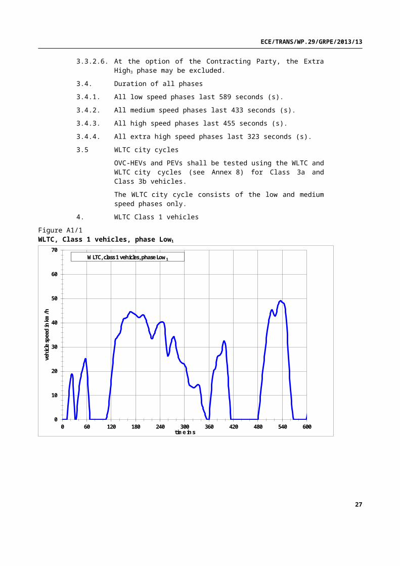
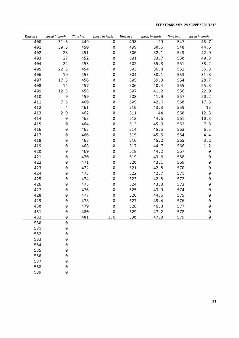
3.1.2. The Low1 phase is described in Figure A1/1 and Table A1/1.
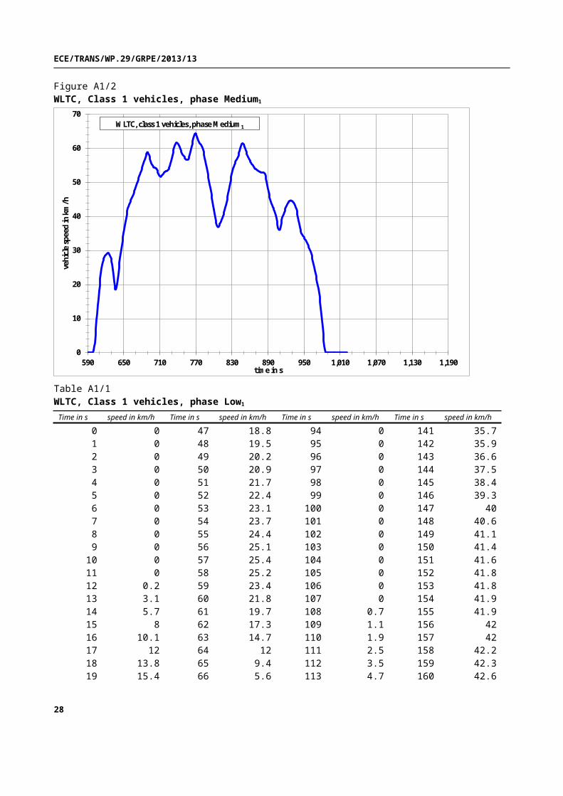
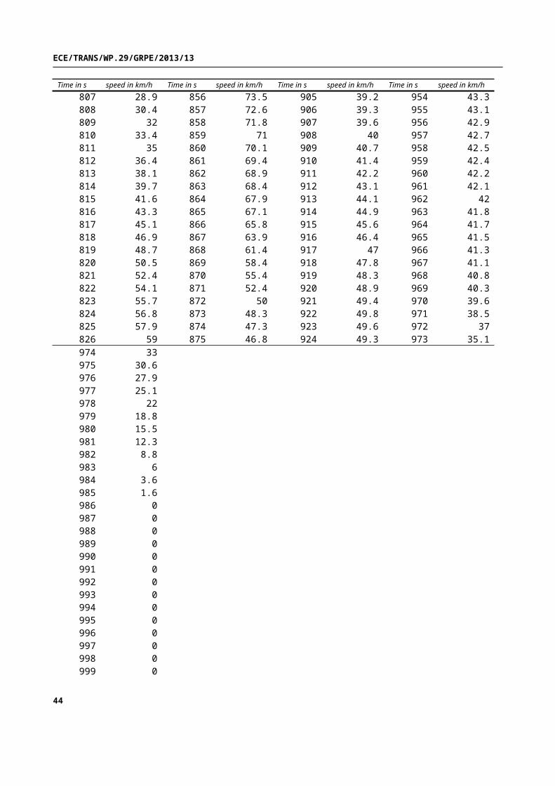
3.1.3. The Medium1 phase is described in Figure A1/2 and Table A1/2.
3.2. Class 2 vehicles
3.2.1. A complete cycle for class 2 vehicles shall consist of a low phase (Low2), a medium phase (Medium2), a high phase (High2) and an extra high phase (Extra High2).
3.2.2. The Low2 phase is described in Figure A1/3 and Table A1/3.
3.2.3. The Medium2 phase is described in Figure A1/4 and Table A1/4.
3.2.4. The High2 phase is described in Figure A1/5 and Table A1/5.
3.2.5. The Extra High2 phase is described in Figure A1/6 and Table A1/6.
3.2.6. At the option of the Contracting Party, the Extra High2 phase may be excluded.
3.3. Class 3 vehicles
Class 3 vehicles are divided into 2 subclasses according to their maximum speed, vmax.
3.3.1. Class 3a vehicles with vmax<120 km/h
3.3.1.1. A complete cycle shall consist of a low phase (Low3) , a medium phase (Medium3-1), a high phase (High3-1) and an extra high phase (Extra High3).
19

ECE/TRANS/WP.29/GRPE/2013/13
3.3.1.2. The Low3 phase is described in Figure A1/7 and Table A1/7.
3.3.1.3. The Medium3-1 phase is described in Figure A1/8 and Table A1/8.
3.3.1.4. The High3-1 phase is described in Figure A1/10 and Table A1/10.
3.3.1.5. The Extra High3 phase is described in Figure A1/12 and Table A1/12.
3.3.1.6. At the option of the Contracting Party, the Extra High3 phase may be excluded.
3.3.2. Class 3b vehicles with vmax ≥120 km/h
3.3.2.1. A complete cycle shall consist of a low phase (Low3) phase, a medium phase (Medium3-2), a high phase (High3-2) and an extra high phase (Extra High3).
3.3.2.2. The Low3 phase is described in Figure A1/7 and Table A1/7.
3.3.2.3. The Medium3-2 phase is described in Figure A1/9 and Table A1/9.
3.3.2.4. The High3-2 phase is described in Figure A1/11 and Table A1/11.
3.3.2.5. The Extra High3 phase is described in Figure A1/12 and Table A1/12.
3.3.2.6. At the option of the Contracting Party, the Extra High3 phase may be excluded.
3.4. Duration of all phases
3.4.1. All low speed phases last 589 seconds (s).
3.4.2. All medium speed phases last 433 seconds (s).
3.4.3. All high speed phases last 455 seconds (s).
3.4.4. All extra high speed phases last 323 seconds (s).
3.5 WLTC city cycles
OVC-HEVs and PEVs shall be tested using the WLTC and WLTC city cycles (see Annex 8) for Class 3a and Class 3b vehicles.
The WLTC city cycle consists of the low and medium speed phases only.
20

ECE/TRANS/WP.29/GRPE/2013/13
4. WLTC Class 1 vehicles
Figure A1/1WLTC, Class 1 vehicles, phase Low1
0
10
20
30
40
50
60
70
0 60 120 180 240 300 360 420 480 540 600
vehi
cle
spee
d in
km
/h
time in s
WLTC, class 1 vehicles, phase Low1
Figure A1/2WLTC, Class 1 vehicles, phase Medium1
0
10
20
30
40
50
60
70
590 650 710 770 830 890 950 1,010 1,070 1,130 1,190
vehi
cle
spee
d in
km
/h
time in s
WLTC, class 1 vehicles, phase Medium1
21

ECE/TRANS/WP.29/GRPE/2013/13
Table A1/1WLTC, Class 1 vehicles, phase Low1
Time in s speed in km/h Time in s speed in km/h Time in s speed in km/h Time in s speed in km/h
0 0 47 18.8 94 0 141 35.71 0 48 19.5 95 0 142 35.92 0 49 20.2 96 0 143 36.63 0 50 20.9 97 0 144 37.54 0 51 21.7 98 0 145 38.45 0 52 22.4 99 0 146 39.36 0 53 23.1 100 0 147 407 0 54 23.7 101 0 148 40.68 0 55 24.4 102 0 149 41.19 0 56 25.1 103 0 150 41.4
10 0 57 25.4 104 0 151 41.611 0 58 25.2 105 0 152 41.812 0.2 59 23.4 106 0 153 41.813 3.1 60 21.8 107 0 154 41.914 5.7 61 19.7 108 0.7 155 41.915 8 62 17.3 109 1.1 156 4216 10.1 63 14.7 110 1.9 157 4217 12 64 12 111 2.5 158 42.218 13.8 65 9.4 112 3.5 159 42.319 15.4 66 5.6 113 4.7 160 42.620 16.7 67 3.1 114 6.1 161 4321 17.7 68 0 115 7.5 162 43.322 18.3 69 0 116 9.4 163 43.723 18.8 70 0 117 11 164 4424 18.9 71 0 118 12.9 165 44.325 18.4 72 0 119 14.5 166 44.526 16.9 73 0 120 16.4 167 44.627 14.3 74 0 121 18 168 44.628 10.8 75 0 122 20 169 44.529 7.1 76 0 123 21.5 170 44.430 4 77 0 124 23.5 171 44.331 0 78 0 125 25 172 44.232 0 79 0 126 26.8 173 44.133 0 80 0 127 28.2 174 4434 0 81 0 128 30 175 43.935 1.5 82 0 129 31.4 176 43.836 3.8 83 0 130 32.5 177 43.737 5.6 84 0 131 33.2 178 43.638 7.5 85 0 132 33.4 179 43.539 9.2 86 0 133 33.7 180 43.440 10.8 87 0 134 33.9 181 43.341 12.4 88 0 135 34.2 182 43.142 13.8 89 0 136 34.4 183 42.943 15.2 90 0 137 34.7 184 42.744 16.3 91 0 138 34.9 185 42.545 17.3 92 0 139 35.2 186 42.346 18 93 0 140 35.4 187 42.2
22

ECE/TRANS/WP.29/GRPE/2013/13
Time in s speed in km/h Time in s speed in km/h Time in s speed in km/h Time in s speed in km/h
188 42.2 237 39.7 286 25.3 335 14.3189 42.2 238 39.9 287 24.9 336 14.3190 42.3 239 40 288 24.5 337 14191 42.4 240 40.1 289 24.2 338 13192 42.5 241 40.2 290 24 339 11.4193 42.7 242 40.3 291 23.8 340 10.2194 42.9 243 40.4 292 23.6 341 8195 43.1 244 40.5 293 23.5 342 7196 43.2 245 40.5 294 23.4 343 6197 43.3 246 40.4 295 23.3 344 5.5198 43.4 247 40.3 296 23.3 345 5199 43.4 248 40.2 297 23.2 346 4.5200 43.2 249 40.1 298 23.1 347 4201 42.9 250 39.7 299 23 348 3.5202 42.6 251 38.8 300 22.8 349 3203 42.2 252 37.4 301 22.5 350 2.5204 41.9 253 35.6 302 22.1 351 2205 41.5 254 33.4 303 21.7 352 1.5206 41 255 31.2 304 21.1 353 1207 40.5 256 29.1 305 20.4 354 0.5208 39.9 257 27.6 306 19.5 355 0209 39.3 258 26.6 307 18.5 356 0210 38.7 259 26.2 308 17.6 357 0211 38.1 260 26.3 309 16.6 358 0212 37.5 261 26.7 310 15.7 359 0213 36.9 262 27.5 311 14.9 360 0214 36.3 263 28.4 312 14.3 361 2.2215 35.7 264 29.4 313 14.1 362 4.5216 35.1 265 30.4 314 14 363 6.6217 34.5 266 31.2 315 13.9 364 8.6218 33.9 267 31.9 316 13.8 365 10.6219 33.6 268 32.5 317 13.7 366 12.5220 33.5 269 33 318 13.6 367 14.4221 33.6 270 33.4 319 13.5 368 16.3222 33.9 271 33.8 320 13.4 369 17.9223 34.3 272 34.1 321 13.3 370 19.1224 34.7 273 34.3 322 13.2 371 19.9225 35.1 274 34.3 323 13.2 372 20.3226 35.5 275 33.9 324 13.2 373 20.5227 35.9 276 33.3 325 13.4 374 20.7228 36.4 277 32.6 326 13.5 375 21229 36.9 278 31.8 327 13.7 376 21.6230 37.4 279 30.7 328 13.8 377 22.6231 37.9 280 29.6 329 14 378 23.7232 38.3 281 28.6 330 14.1 379 24.8233 38.7 282 27.8 331 14.3 380 25.7234 39.1 283 27 332 14.4 381 26.2235 39.3 284 26.4 333 14.4 382 26.4236 39.5 285 25.8 334 14.4 383 26.4
23

ECE/TRANS/WP.29/GRPE/2013/13
Time in s speed in km/h Time in s speed in km/h Time in s speed in km/h Time in s speed in km/h
384 26.4 433 0 482 3.1 531 48.2385 26.5 434 0 483 4.6 532 48.5386 26.6 435 0 484 6.1 533 48.7387 26.8 436 0 485 7.8 534 48.9388 26.9 437 0 486 9.5 535 49.1389 27.2 438 0 487 11.3 536 49.1390 27.5 439 0 488 13.2 537 49391 28 440 0 489 15 538 48.8392 28.8 441 0 490 16.8 539 48.6393 29.9 442 0 491 18.4 540 48.5394 31 443 0 492 20.1 541 48.4395 31.9 444 0 493 21.6 542 48.3396 32.5 445 0 494 23.1 543 48.2397 32.6 446 0 495 24.6 544 48.1398 32.4 447 0 496 26 545 47.5399 32 448 0 497 27.5 546 46.7400 31.3 449 0 498 29 547 45.7401 30.3 450 0 499 30.6 548 44.6402 28 451 0 500 32.1 549 42.9403 27 452 0 501 33.7 550 40.8404 24 453 0 502 35.3 551 38.2405 22.5 454 0 503 36.8 552 35.3406 19 455 0 504 38.1 553 31.8407 17.5 456 0 505 39.3 554 28.7408 14 457 0 506 40.4 555 25.8409 12.5 458 0 507 41.2 556 22.9410 9 459 0 508 41.9 557 20.2411 7.5 460 0 509 42.6 558 17.3412 4 461 0 510 43.3 559 15413 2.9 462 0 511 44 560 12.3414 0 463 0 512 44.6 561 10.3415 0 464 0 513 45.3 562 7.8416 0 465 0 514 45.5 563 6.5417 0 466 0 515 45.5 564 4.4418 0 467 0 516 45.2 565 3.2419 0 468 0 517 44.7 566 1.2420 0 469 0 518 44.2 567 0421 0 470 0 519 43.6 568 0422 0 471 0 520 43.1 569 0423 0 472 0 521 42.8 570 0424 0 473 0 522 42.7 571 0425 0 474 0 523 42.8 572 0426 0 475 0 524 43.3 573 0427 0 476 0 525 43.9 574 0428 0 477 0 526 44.6 575 0429 0 478 0 527 45.4 576 0430 0 479 0 528 46.3 577 0431 0 480 0 529 47.2 578 0432 0 481 1.6 530 47.8 579 0
24

ECE/TRANS/WP.29/GRPE/2013/13
Time in s speed in km/h Time in s speed in km/h Time in s speed in km/h Time in s speed in km/h
580 0581 0582 0583 0584 0585 0586 0587 0588 0589 0
25

ECE/TRANS/WP.29/GRPE/2013/13
Table A1/2WLTC, Class 1 vehicles, phase Medium1
Time in s speed in km/h Time in s speed in km/h Time in s speed in km/h Time in s speed in km/h
590 0 637 18.4 684 56.2 731 57.9591 0 638 19 685 56.7 732 58.8592 0 639 20.1 686 57.3 733 59.6593 0 640 21.5 687 57.9 734 60.3594 0 641 23.1 688 58.4 735 60.9595 0 642 24.9 689 58.8 736 61.3596 0 643 26.4 690 58.9 737 61.7597 0 644 27.9 691 58.4 738 61.8598 0 645 29.2 692 58.1 739 61.8599 0 646 30.4 693 57.6 740 61.6600 0.6 647 31.6 694 56.9 741 61.2601 1.9 648 32.8 695 56.3 742 60.8602 2.7 649 34 696 55.7 743 60.4603 5.2 650 35.1 697 55.3 744 59.9604 7 651 36.3 698 55 745 59.4605 9.6 652 37.4 699 54.7 746 58.9606 11.4 653 38.6 700 54.5 747 58.6607 14.1 654 39.6 701 54.4 748 58.2608 15.8 655 40.6 702 54.3 749 57.9609 18.2 656 41.6 703 54.2 750 57.7610 19.7 657 42.4 704 54.1 751 57.5611 21.8 658 43 705 53.8 752 57.2612 23.2 659 43.6 706 53.5 753 57613 24.7 660 44 707 53 754 56.8614 25.8 661 44.4 708 52.6 755 56.6615 26.7 662 44.8 709 52.2 756 56.6616 27.2 663 45.2 710 51.9 757 56.7617 27.7 664 45.6 711 51.7 758 57.1618 28.1 665 46 712 51.7 759 57.6619 28.4 666 46.5 713 51.8 760 58.2620 28.7 667 47 714 52 761 59621 29 668 47.5 715 52.3 762 59.8622 29.2 669 48 716 52.6 763 60.6623 29.4 670 48.6 717 52.9 764 61.4624 29.4 671 49.1 718 53.1 765 62.2625 29.3 672 49.7 719 53.2 766 62.9626 28.9 673 50.2 720 53.3 767 63.5627 28.5 674 50.8 721 53.3 768 64.2628 28.1 675 51.3 722 53.4 769 64.4629 27.6 676 51.8 723 53.5 770 64.4630 26.9 677 52.3 724 53.7 771 64631 26 678 52.9 725 54 772 63.5632 24.6 679 53.4 726 54.4 773 62.9633 22.8 680 54 727 54.9 774 62.4634 21 681 54.5 728 55.6 775 62635 19.5 682 55.1 729 56.3 776 61.6636 18.6 683 55.6 730 57.1 777 61.4
26
ECE/TRANS/WP.29/GRPE/2013/13
Time in s speed in km/h Time in s speed in km/h Time in s speed in km/h Time in s speed in km/h
778 61.2 827 49.7 876 53.2 925 44.4779 61 828 50.6 877 53.1 926 44.5780 60.7 829 51.6 878 53 927 44.6781 60.2 830 52.5 879 53 928 44.7782 59.6 831 53.3 880 53 929 44.6783 58.9 832 54.1 881 53 930 44.5784 58.1 833 54.7 882 53 931 44.4785 57.2 834 55.3 883 53 932 44.2786 56.3 835 55.7 884 52.8 933 44.1787 55.3 836 56.1 885 52.5 934 43.7788 54.4 837 56.4 886 51.9 935 43.3789 53.4 838 56.7 887 51.1 936 42.8790 52.4 839 57.1 888 50.2 937 42.3791 51.4 840 57.5 889 49.2 938 41.6792 50.4 841 58 890 48.2 939 40.7793 49.4 842 58.7 891 47.3 940 39.8794 48.5 843 59.3 892 46.4 941 38.8795 47.5 844 60 893 45.6 942 37.8796 46.5 845 60.6 894 45 943 36.9797 45.4 846 61.3 895 44.3 944 36.1798 44.3 847 61.5 896 43.8 945 35.5799 43.1 848 61.5 897 43.3 946 35800 42 849 61.4 898 42.8 947 34.7801 40.8 850 61.2 899 42.4 948 34.4802 39.7 851 60.5 900 42 949 34.1803 38.8 852 60 901 41.6 950 33.9804 38.1 853 59.5 902 41.1 951 33.6805 37.4 854 58.9 903 40.3 952 33.3806 37.1 855 58.4 904 39.5 953 33807 36.9 856 57.9 905 38.6 954 32.7808 37 857 57.5 906 37.7 955 32.3809 37.5 858 57.1 907 36.7 956 31.9810 37.8 859 56.7 908 36.2 957 31.5811 38.2 860 56.4 909 36 958 31812 38.6 861 56.1 910 36.2 959 30.6813 39.1 862 55.8 911 37 960 30.2814 39.6 863 55.5 912 38 961 29.7815 40.1 864 55.3 913 39 962 29.1816 40.7 865 55 914 39.7 963 28.4817 41.3 866 54.7 915 40.2 964 27.6818 41.9 867 54.4 916 40.7 965 26.8819 42.7 868 54.2 917 41.2 966 26820 43.4 869 54 918 41.7 967 25.1821 44.2 870 53.9 919 42.2 968 24.2822 45 871 53.7 920 42.7 969 23.3823 45.9 872 53.6 921 43.2 970 22.4824 46.8 873 53.5 922 43.6 971 21.5825 47.7 874 53.4 923 44 972 20.6826 48.7 875 53.3 924 44.2 973 19.7
27
ECE/TRANS/WP.29/GRPE/2013/13
Time in s speed in km/h Time in s speed in km/h Time in s speed in km/h Time in s speed in km/h
974 18.8975 17.7976 16.4977 14.9978 13.2979 11.3980 9.4981 7.5982 5.6983 3.7984 1.9985 1986 0987 0988 0989 0990 0991 0992 0993 0994 0995 0996 0997 0998 0999 0
1000 01001 01002 01003 01004 01005 01006 01007 01008 01009 01010 01011 01012 01013 01014 01015 01016 01017 01018 01019 01020 01021 01022 0
28

ECE/TRANS/WP.29/GRPE/2013/13
5. WLTC for Class 2 vehicles
Figure A1/3WLTC, Class 2 vehicles, phase Low2
0
10
20
30
40
50
60
70
80
90
100
110
120
130
0 60 120 180 240 300 360 420 480 540 600
vehi
cle
spee
d in
km
/h
time in s
WLTC, class2 vehicles, phase Low2
Figure A1/4WLTC, Class 2 vehicles, phase Medium2
0
10
20
30
40
50
60
70
80
90
100
110
120
130
580 640 700 760 820 880 940 1,000
vehi
cle
spee
d in
km
/h
time in s
WLTC, class 2 vehicles, phase Medium2
29

ECE/TRANS/WP.29/GRPE/2013/13
Figure A1/5WLTC, Class 2 vehicles, phase High2
0
10
20
30
40
50
60
70
80
90
100
110
120
130
1,020 1,080 1,140 1,200 1,260 1,320 1,380 1,440 1,500
vehi
cle
spee
d in
km
/h
time in s
WLTC, class2 vehicles, phase High2
Figure A1/6WLTC, Class 2 vehicles, phase Extra High2
0
10
20
30
40
50
60
70
80
90
100
110
120
130
1,470 1,530 1,590 1,650 1,710 1,770 1,830
vehi
cle
spee
d in
km
/h
time in s
WLTC, class 2 vehicles, phase Extra High2
30
ECE/TRANS/WP.29/GRPE/2013/13
Table A1/3WLTC, Class 2 vehicles, phase Low2
Time in s speed in km/h Time in s speed in km/h Time in s speed in km/h Time in s speed in km/h
0 0 47 11.6 94 0 141 36.81 0 48 12.4 95 0 142 35.12 0 49 13.2 96 0 143 32.23 0 50 14.2 97 0 144 31.14 0 51 14.8 98 0 145 30.85 0 52 14.7 99 0 146 29.76 0 53 14.4 100 0 147 29.47 0 54 14.1 101 0 148 298 0 55 13.6 102 0 149 28.59 0 56 13 103 0 150 26
10 0 57 12.4 104 0 151 23.411 0 58 11.8 105 0 152 20.712 0 59 11.2 106 0 153 17.413 1.2 60 10.6 107 0.8 154 15.214 2.6 61 9.9 108 1.4 155 13.515 4.9 62 9 109 2.3 156 1316 7.3 63 8.2 110 3.5 157 12.417 9.4 64 7 111 4.7 158 12.318 11.4 65 4.8 112 5.9 159 12.219 12.7 66 2.3 113 7.4 160 12.320 13.3 67 0 114 9.2 161 12.421 13.4 68 0 115 11.7 162 12.522 13.3 69 0 116 13.5 163 12.723 13.1 70 0 117 15 164 12.824 12.5 71 0 118 16.2 165 13.225 11.1 72 0 119 16.8 166 14.326 8.9 73 0 120 17.5 167 16.527 6.2 74 0 121 18.8 168 19.428 3.8 75 0 122 20.3 169 21.729 1.8 76 0 123 22 170 23.130 0 77 0 124 23.6 171 23.531 0 78 0 125 24.8 172 24.232 0 79 0 126 25.6 173 24.833 0 80 0 127 26.3 174 25.434 1.5 81 0 128 27.2 175 25.835 2.8 82 0 129 28.3 176 26.536 3.6 83 0 130 29.6 177 27.237 4.5 84 0 131 30.9 178 28.338 5.3 85 0 132 32.2 179 29.939 6 86 0 133 33.4 180 32.440 6.6 87 0 134 35.1 181 35.141 7.3 88 0 135 37.2 182 37.542 7.9 89 0 136 38.7 183 39.243 8.6 90 0 137 39 184 40.544 9.3 91 0 138 40.1 185 41.445 10 92 0 139 40.4 186 4246 10.8 93 0 140 39.7 187 42.5
31

ECE/TRANS/WP.29/GRPE/2013/13
Time in s speed in km/h Time in s speed in km/h Time in s speed in km/h Time in s speed in km/h
188 43.2 237 33.5 286 32.5 335 25189 44.4 238 35.8 287 30.9 336 24.6190 45.9 239 37.6 288 28.6 337 23.9191 47.6 240 38.8 289 25.9 338 23192 49 241 39.6 290 23.1 339 21.8193 50 242 40.1 291 20.1 340 20.7194 50.2 243 40.9 292 17.3 341 19.6195 50.1 244 41.8 293 15.1 342 18.7196 49.8 245 43.3 294 13.7 343 18.1197 49.4 246 44.7 295 13.4 344 17.5198 48.9 247 46.4 296 13.9 345 16.7199 48.5 248 47.9 297 15 346 15.4200 48.3 249 49.6 298 16.3 347 13.6201 48.2 250 49.6 299 17.4 348 11.2202 47.9 251 48.8 300 18.2 349 8.6203 47.1 252 48 301 18.6 350 6204 45.5 253 47.5 302 19 351 3.1205 43.2 254 47.1 303 19.4 352 1.2206 40.6 255 46.9 304 19.8 353 0207 38.5 256 45.8 305 20.1 354 0208 36.9 257 45.8 306 20.5 355 0209 35.9 258 45.8 307 20.2 356 0210 35.3 259 45.9 308 18.6 357 0211 34.8 260 46.2 309 16.5 358 0212 34.5 261 46.4 310 14.4 359 0213 34.2 262 46.6 311 13.4 360 1.4214 34 263 46.8 312 12.9 361 3.2215 33.8 264 47 313 12.7 362 5.6216 33.6 265 47.3 314 12.4 363 8.1217 33.5 266 47.5 315 12.4 364 10.3218 33.5 267 47.9 316 12.8 365 12.1219 33.4 268 48.3 317 14.1 366 12.6220 33.3 269 48.3 318 16.2 367 13.6221 33.3 270 48.2 319 18.8 368 14.5222 33.2 271 48 320 21.9 369 15.6223 33.1 272 47.7 321 25 370 16.8224 33 273 47.2 322 28.4 371 18.2225 32.9 274 46.5 323 31.3 372 19.6226 32.8 275 45.2 324 34 373 20.9227 32.7 276 43.7 325 34.6 374 22.3228 32.5 277 42 326 33.9 375 23.8229 32.3 278 40.4 327 31.9 376 25.4230 31.8 279 39 328 30 377 27231 31.4 280 37.7 329 29 378 28.6232 30.9 281 36.4 330 27.9 379 30.2233 30.6 282 35.2 331 27.1 380 31.2234 30.6 283 34.3 332 26.4 381 31.2235 30.7 284 33.8 333 25.9 382 30.7236 32 285 33.3 334 25.5 383 29.5
32

ECE/TRANS/WP.29/GRPE/2013/13
Time in s speed in km/h Time in s speed in km/h Time in s speed in km/h Time in s speed in km/h
384 28.6 433 0 482 2.5 531 26385 27.7 434 0 483 5.2 532 26.5386 26.9 435 0 484 7.9 533 26.9387 26.1 436 0 485 10.3 534 27.3388 25.4 437 0 486 12.7 535 27.9389 24.6 438 0 487 15 536 30.3390 23.6 439 0 488 17.4 537 33.2391 22.6 440 0 489 19.7 538 35.4392 21.7 441 0 490 21.9 539 38393 20.7 442 0 491 24.1 540 40.1394 19.8 443 0 492 26.2 541 42.7395 18.8 444 0 493 28.1 542 44.5396 17.7 445 0 494 29.7 543 46.3397 16.6 446 0 495 31.3 544 47.6398 15.6 447 0 496 33 545 48.8399 14.8 448 0 497 34.7 546 49.7400 14.3 449 0 498 36.3 547 50.6401 13.8 450 0 499 38.1 548 51.4402 13.4 451 0 500 39.4 549 51.4403 13.1 452 0 501 40.4 550 50.2404 12.8 453 0 502 41.2 551 47.1405 12.3 454 0 503 42.1 552 44.5406 11.6 455 0 504 43.2 553 41.5407 10.5 456 0 505 44.3 554 38.5408 9 457 0 506 45.7 555 35.5409 7.2 458 0 507 45.4 556 32.5410 5.2 459 0 508 44.5 557 29.5411 2.9 460 0 509 42.5 558 26.5412 1.2 461 0 510 39.5 559 23.5413 0 462 0 511 36.5 560 20.4414 0 463 0 512 33.5 561 17.5415 0 464 0 513 30.4 562 14.5416 0 465 0 514 27 563 11.5417 0 466 0 515 23.6 564 8.5418 0 467 0 516 21 565 5.6419 0 468 0 517 19.5 566 2.6420 0 469 0 518 17.6 567 0421 0 470 0 519 16.1 568 0422 0 471 0 520 14.5 569 0423 0 472 0 521 13.5 570 0424 0 473 0 522 13.7 571 0425 0 474 0 523 16 572 0426 0 475 0 524 18.1 573 0427 0 476 0 525 20.8 574 0428 0 477 0 526 21.5 575 0429 0 478 0 527 22.5 576 0430 0 479 0 528 23.4 577 0431 0 480 0 529 24.5 578 0432 0 481 1.4 530 25.6 579 0
33

ECE/TRANS/WP.29/GRPE/2013/13
Time in s speed in km/h Time in s speed in km/h Time in s speed in km/h Time in s speed in km/h
580 0581 0582 0583 0584 0585 0586 0587 0588 0589 0
34

ECE/TRANS/WP.29/GRPE/2013/13
Table A1/4WLTC, Class 2 vehicles, phase Medium2
Time in s speed in km/h Time in s speed in km/h Time in s speed in km/h Time in s speed in km/h
590 0 637 38.6 684 59.3 731 55.3591 0 638 39.8 685 60.2 732 55.1592 0 639 40.6 686 61.3 733 54.8593 0 640 41.1 687 62.4 734 54.6594 0 641 41.9 688 63.4 735 54.5595 0 642 42.8 689 64.4 736 54.3596 0 643 44.3 690 65.4 737 53.9597 0 644 45.7 691 66.3 738 53.4598 0 645 47.4 692 67.2 739 52.6599 0 646 48.9 693 68 740 51.5600 0 647 50.6 694 68.8 741 50.2601 1.6 648 52 695 69.5 742 48.7602 3.6 649 53.7 696 70.1 743 47603 6.3 650 55 697 70.6 744 45.1604 9 651 56.8 698 71 745 43605 11.8 652 58 699 71.6 746 40.6606 14.2 653 59.8 700 72.2 747 38.1607 16.6 654 61.1 701 72.8 748 35.4608 18.5 655 62.4 702 73.5 749 32.7609 20.8 656 63 703 74.1 750 30610 23.4 657 63.5 704 74.3 751 27.5611 26.9 658 63 705 74.3 752 25.3612 30.3 659 62 706 73.7 753 23.4613 32.8 660 60.4 707 71.9 754 22614 34.1 661 58.6 708 70.5 755 20.8615 34.2 662 56.7 709 68.9 756 19.8616 33.6 663 55 710 67.4 757 18.9617 32.1 664 53.7 711 66 758 18618 30 665 52.7 712 64.7 759 17619 27.5 666 51.9 713 63.7 760 16.1620 25.1 667 51.4 714 62.9 761 15.5621 22.8 668 51 715 62.2 762 14.4622 20.5 669 50.7 716 61.7 763 14.9623 17.9 670 50.6 717 61.2 764 15.9624 15.1 671 50.8 718 60.7 765 17.1625 13.4 672 51.2 719 60.3 766 18.3626 12.8 673 51.7 720 59.9 767 19.4627 13.7 674 52.3 721 59.6 768 20.4628 16 675 53.1 722 59.3 769 21.2629 18.1 676 53.8 723 59 770 21.9630 20.8 677 54.5 724 58.6 771 22.7631 23.7 678 55.1 725 58 772 23.4632 26.5 679 55.9 726 57.5 773 24.2633 29.3 680 56.5 727 56.9 774 24.3634 32 681 57.1 728 56.3 775 24.2635 34.5 682 57.8 729 55.9 776 24.1636 36.8 683 58.5 730 55.6 777 23.8
35

ECE/TRANS/WP.29/GRPE/2013/13
Time in s speed in km/h Time in s speed in km/h Time in s speed in km/h Time in s speed in km/h
778 23 827 59.9 876 46.9 925 49779 22.6 828 60.7 877 47.1 926 48.5780 21.7 829 61.4 878 47.5 927 48781 21.3 830 62 879 47.8 928 47.5782 20.3 831 62.5 880 48.3 929 47783 19.1 832 62.9 881 48.8 930 46.9784 18.1 833 63.2 882 49.5 931 46.8785 16.9 834 63.4 883 50.2 932 46.8786 16 835 63.7 884 50.8 933 46.8787 14.8 836 64 885 51.4 934 46.9788 14.5 837 64.4 886 51.8 935 46.9789 13.7 838 64.9 887 51.9 936 46.9790 13.5 839 65.5 888 51.7 937 46.9791 12.9 840 66.2 889 51.2 938 46.9792 12.7 841 67 890 50.4 939 46.8793 12.5 842 67.8 891 49.2 940 46.6794 12.5 843 68.6 892 47.7 941 46.4795 12.6 844 69.4 893 46.3 942 46796 13 845 70.1 894 45.1 943 45.5797 13.6 846 70.9 895 44.2 944 45798 14.6 847 71.7 896 43.7 945 44.5799 15.7 848 72.5 897 43.4 946 44.2800 17.1 849 73.2 898 43.1 947 43.9801 18.7 850 73.8 899 42.5 948 43.7802 20.2 851 74.4 900 41.8 949 43.6803 21.9 852 74.7 901 41.1 950 43.6804 23.6 853 74.7 902 40.3 951 43.5805 25.4 854 74.6 903 39.7 952 43.5806 27.1 855 74.2 904 39.3 953 43.4807 28.9 856 73.5 905 39.2 954 43.3808 30.4 857 72.6 906 39.3 955 43.1809 32 858 71.8 907 39.6 956 42.9810 33.4 859 71 908 40 957 42.7811 35 860 70.1 909 40.7 958 42.5812 36.4 861 69.4 910 41.4 959 42.4813 38.1 862 68.9 911 42.2 960 42.2814 39.7 863 68.4 912 43.1 961 42.1815 41.6 864 67.9 913 44.1 962 42816 43.3 865 67.1 914 44.9 963 41.8817 45.1 866 65.8 915 45.6 964 41.7818 46.9 867 63.9 916 46.4 965 41.5819 48.7 868 61.4 917 47 966 41.3820 50.5 869 58.4 918 47.8 967 41.1821 52.4 870 55.4 919 48.3 968 40.8822 54.1 871 52.4 920 48.9 969 40.3823 55.7 872 50 921 49.4 970 39.6824 56.8 873 48.3 922 49.8 971 38.5825 57.9 874 47.3 923 49.6 972 37826 59 875 46.8 924 49.3 973 35.1
36

ECE/TRANS/WP.29/GRPE/2013/13
Time in s speed in km/h Time in s speed in km/h Time in s speed in km/h Time in s speed in km/h
974 33975 30.6976 27.9977 25.1978 22979 18.8980 15.5981 12.3982 8.8983 6984 3.6985 1.6986 0987 0988 0989 0990 0991 0992 0993 0994 0995 0996 0997 0998 0999 0
1000 01001 01002 01003 01004 01005 01006 01007 01008 01009 01010 01011 01012 01013 01014 01015 01016 01017 01018 01019 01020 01021 01022 0
37

ECE/TRANS/WP.29/GRPE/2013/13
Table A1/5WLTC, Class 2 vehicles, phase High2
Time in s speed in km/h Time in s speed in km/h Time in s speed in km/h Time in s speed in km/h
1023 0 1070 46 1117 73.9 1164 71.71024 0 1071 46.4 1118 74.9 1165 69.91025 0 1072 47 1119 75.7 1166 67.91026 0 1073 47.4 1120 76.4 1167 65.71027 1.1 1074 48 1121 77.1 1168 63.51028 3 1075 48.4 1122 77.6 1169 61.21029 5.7 1076 49 1123 78 1170 591030 8.4 1077 49.4 1124 78.2 1171 56.81031 11.1 1078 50 1125 78.4 1172 54.71032 14 1079 50.4 1126 78.5 1173 52.71033 17 1080 50.8 1127 78.5 1174 50.91034 20.1 1081 51.1 1128 78.6 1175 49.41035 22.7 1082 51.3 1129 78.7 1176 48.11036 23.6 1083 51.3 1130 78.9 1177 47.11037 24.5 1084 51.3 1131 79.1 1178 46.51038 24.8 1085 51.3 1132 79.4 1179 46.31039 25.1 1086 51.3 1133 79.8 1180 46.51040 25.3 1087 51.3 1134 80.1 1181 47.21041 25.5 1088 51.3 1135 80.5 1182 48.31042 25.7 1089 51.4 1136 80.8 1183 49.71043 25.8 1090 51.6 1137 81 1184 51.31044 25.9 1091 51.8 1138 81.2 1185 531045 26 1092 52.1 1139 81.3 1186 54.91046 26.1 1093 52.3 1140 81.2 1187 56.71047 26.3 1094 52.6 1141 81 1188 58.61048 26.5 1095 52.8 1142 80.6 1189 60.21049 26.8 1096 52.9 1143 80 1190 61.61050 27.1 1097 53 1144 79.1 1191 62.21051 27.5 1098 53 1145 78 1192 62.51052 28 1099 53 1146 76.8 1193 62.81053 28.6 1100 53.1 1147 75.5 1194 62.91054 29.3 1101 53.2 1148 74.1 1195 631055 30.4 1102 53.3 1149 72.9 1196 631056 31.8 1103 53.4 1150 71.9 1197 63.11057 33.7 1104 53.5 1151 71.2 1198 63.21058 35.8 1105 53.7 1152 70.9 1199 63.31059 37.8 1106 55 1153 71 1200 63.51060 39.5 1107 56.8 1154 71.5 1201 63.71061 40.8 1108 58.8 1155 72.3 1202 63.91062 41.8 1109 60.9 1156 73.2 1203 64.11063 42.4 1110 63 1157 74.1 1204 64.31064 43 1111 65 1158 74.9 1205 66.11065 43.4 1112 66.9 1159 75.4 1206 67.91066 44 1113 68.6 1160 75.5 1207 69.71067 44.4 1114 70.1 1161 75.2 1208 71.41068 45 1115 71.5 1162 74.5 1209 73.11069 45.4 1116 72.8 1163 73.3 1210 74.7
38

ECE/TRANS/WP.29/GRPE/2013/13
Time in s speed in km/h Time in s speed in km/h Time in s speed in km/h Time in s speed in km/h
1211 76.2 1260 35.4 1309 72.3 1358 70.81212 77.5 1261 32.7 1310 71.9 1359 70.81213 78.6 1262 30 1311 71.3 1360 70.91214 79.7 1263 29.9 1312 70.9 1361 70.91215 80.6 1264 30 1313 70.5 1362 70.91216 81.5 1265 30.2 1314 70 1363 70.91217 82.2 1266 30.4 1315 69.6 1364 711218 83 1267 30.6 1316 69.2 1365 711219 83.7 1268 31.6 1317 68.8 1366 71.11220 84.4 1269 33 1318 68.4 1367 71.21221 84.9 1270 33.9 1319 67.9 1368 71.31222 85.1 1271 34.8 1320 67.5 1369 71.41223 85.2 1272 35.7 1321 67.2 1370 71.51224 84.9 1273 36.6 1322 66.8 1371 71.71225 84.4 1274 37.5 1323 65.6 1372 71.81226 83.6 1275 38.4 1324 63.3 1373 71.91227 82.7 1276 39.3 1325 60.2 1374 71.91228 81.5 1277 40.2 1326 56.2 1375 71.91229 80.1 1278 40.8 1327 52.2 1376 71.91230 78.7 1279 41.7 1328 48.4 1377 71.91231 77.4 1280 42.4 1329 45 1378 71.91232 76.2 1281 43.1 1330 41.6 1379 71.91233 75.4 1282 43.6 1331 38.6 1380 721234 74.8 1283 44.2 1332 36.4 1381 72.11235 74.3 1284 44.8 1333 34.8 1382 72.41236 73.8 1285 45.5 1334 34.2 1383 72.71237 73.2 1286 46.3 1335 34.7 1384 73.11238 72.4 1287 47.2 1336 36.3 1385 73.41239 71.6 1288 48.1 1337 38.5 1386 73.81240 70.8 1289 49.1 1338 41 1387 741241 69.9 1290 50 1339 43.7 1388 74.11242 67.9 1291 51 1340 46.5 1389 741243 65.7 1292 51.9 1341 49.1 1390 731244 63.5 1293 52.7 1342 51.6 1391 721245 61.2 1294 53.7 1343 53.9 1392 711246 59 1295 55 1344 56 1393 701247 56.8 1296 56.8 1345 57.9 1394 691248 54.7 1297 58.8 1346 59.7 1395 681249 52.7 1298 60.9 1347 61.2 1396 67.71250 50.9 1299 63 1348 62.5 1397 66.71251 49.4 1300 65 1349 63.5 1398 66.61252 48.1 1301 66.9 1350 64.3 1399 66.71253 47.1 1302 68.6 1351 65.3 1400 66.81254 46.5 1303 70.1 1352 66.3 1401 66.91255 46.3 1304 71 1353 67.3 1402 66.91256 45.1 1305 71.8 1354 68.3 1403 66.91257 43 1306 72.8 1355 69.3 1404 66.91258 40.6 1307 72.9 1356 70.3 1405 66.91259 38.1 1308 73 1357 70.8 1406 66.9
39

ECE/TRANS/WP.29/GRPE/2013/13
Time in s speed in km/h Time in s speed in km/h Time in s speed in km/h Time in s speed in km/h
1407 66.9 1456 01408 67 1457 01409 67.1 1458 01410 67.3 1459 01411 67.5 1460 01412 67.8 1461 01413 68.2 1462 01414 68.6 1463 01415 69 1464 01416 69.3 1465 01417 69.3 1466 01418 69.2 1467 01419 68.8 1468 01420 68.2 1469 01421 67.6 1470 01422 67.4 1471 01423 67.2 1472 01424 66.9 1473 01425 66.3 1474 01426 65.4 1475 01427 64 1476 01428 62.4 1477 01429 60.61430 58.61431 56.71432 54.81433 531434 51.31435 49.61436 47.81437 45.51438 42.81439 39.81440 36.51441 331442 29.51443 25.81444 22.11445 18.61446 15.31447 12.41448 9.61449 6.61450 3.81451 1.61452 01453 01454 01455 0
40

ECE/TRANS/WP.29/GRPE/2013/13
Table A1/6WLTC, Class 2 vehicles, phase Extra High2
Time in s speed in km/h Time in s speed in km/h Time in s speed in km/h Time in s speed in km/h
1478 0 1525 63.4 1572 107.4 1619 113.71479 1.1 1526 64.5 1573 108.7 1620 114.11480 2.3 1527 65.7 1574 109.9 1621 114.41481 4.6 1528 66.9 1575 111.2 1622 114.61482 6.5 1529 68.1 1576 112.3 1623 114.71483 8.9 1530 69.1 1577 113.4 1624 114.71484 10.9 1531 70 1578 114.4 1625 114.71485 13.5 1532 70.9 1579 115.3 1626 114.61486 15.2 1533 71.8 1580 116.1 1627 114.51487 17.6 1534 72.6 1581 116.8 1628 114.51488 19.3 1535 73.4 1582 117.4 1629 114.51489 21.4 1536 74 1583 117.7 1630 114.71490 23 1537 74.7 1584 118.2 1631 1151491 25 1538 75.2 1585 118.1 1632 115.61492 26.5 1539 75.7 1586 117.7 1633 116.41493 28.4 1540 76.4 1587 117 1634 117.31494 29.8 1541 77.2 1588 116.1 1635 118.21495 31.7 1542 78.2 1589 115.2 1636 118.81496 33.7 1543 78.9 1590 114.4 1637 119.31497 35.8 1544 79.9 1591 113.6 1638 119.61498 38.1 1545 81.1 1592 113 1639 119.71499 40.5 1546 82.4 1593 112.6 1640 119.51500 42.2 1547 83.7 1594 112.2 1641 119.31501 43.5 1548 85.4 1595 111.9 1642 119.21502 44.5 1549 87 1596 111.6 1643 1191503 45.2 1550 88.3 1597 111.2 1644 118.81504 45.8 1551 89.5 1598 110.7 1645 118.81505 46.6 1552 90.5 1599 110.1 1646 118.81506 47.4 1553 91.3 1600 109.3 1647 118.81507 48.5 1554 92.2 1601 108.4 1648 118.81508 49.7 1555 93 1602 107.4 1649 118.91509 51.3 1556 93.8 1603 106.7 1650 1191510 52.9 1557 94.6 1604 106.3 1651 1191511 54.3 1558 95.3 1605 106.2 1652 119.11512 55.6 1559 95.9 1606 106.4 1653 119.21513 56.8 1560 96.6 1607 107 1654 119.41514 57.9 1561 97.4 1608 107.5 1655 119.61515 58.9 1562 98.1 1609 107.9 1656 119.91516 59.7 1563 98.7 1610 108.4 1657 120.11517 60.3 1564 99.5 1611 108.9 1658 120.31518 60.7 1565 100.3 1612 109.5 1659 120.41519 60.9 1566 101.1 1613 110.2 1660 120.51520 61 1567 101.9 1614 110.9 1661 120.51521 61.1 1568 102.8 1615 111.6 1662 120.51522 61.4 1569 103.8 1616 112.2 1663 120.51523 61.8 1570 105 1617 112.8 1664 120.41524 62.5 1571 106.1 1618 113.3 1665 120.3
41

ECE/TRANS/WP.29/GRPE/2013/13
Time in s speed in km/h Time in s speed in km/h Time in s speed in km/h Time in s speed in km/h
1666 120.1 1715 120.4 1764 82.61667 119.9 1716 120.8 1765 81.91668 119.6 1717 121.1 1766 81.11669 119.5 1718 121.6 1767 801670 119.4 1719 121.8 1768 78.71671 119.3 1720 122.1 1769 76.91672 119.3 1721 122.4 1770 74.61673 119.4 1722 122.7 1771 721674 119.5 1723 122.8 1772 691675 119.5 1724 123.1 1773 65.61676 119.6 1725 123.1 1774 62.11677 119.6 1726 122.8 1775 58.51678 119.6 1727 122.3 1776 54.71679 119.4 1728 121.3 1777 50.91680 119.3 1729 119.9 1778 47.31681 119 1730 118.1 1779 43.81682 118.8 1731 115.9 1780 40.41683 118.7 1732 113.5 1781 37.41684 118.8 1733 111.1 1782 34.31685 119 1734 108.6 1783 31.31686 119.2 1735 106.2 1784 28.31687 119.6 1736 104 1785 25.21688 120 1737 101.1 1786 221689 120.3 1738 98.3 1787 18.91690 120.5 1739 95.7 1788 16.11691 120.7 1740 93.5 1789 13.41692 120.9 1741 91.5 1790 11.11693 121 1742 90.7 1791 8.91694 121.1 1743 90.4 1792 6.91695 121.2 1744 90.2 1793 4.91696 121.3 1745 90.2 1794 2.81697 121.4 1746 90.1 1795 01698 121.5 1747 90 1796 01699 121.5 1748 89.8 1797 01700 121.5 1749 89.6 1798 01701 121.4 1750 89.4 1799 01702 121.3 1751 89.2 1800 01703 121.1 1752 88.91704 120.9 1753 88.51705 120.6 1754 88.11706 120.4 1755 87.61707 120.2 1756 87.11708 120.1 1757 86.61709 119.9 1758 86.11710 119.8 1759 85.51711 119.8 1760 851712 119.9 1761 84.41713 120 1762 83.81714 120.2 1763 83.2
42

ECE/TRANS/WP.29/GRPE/2013/13
6. WLTC for Class 3 vehicles
Figure A1/7WLTC, Class 3 vehicles, phase Low3
0
20
40
60
80
100
120
140
0 60 120 180 240 300 360 420 480 540 600
vehi
cle
spee
d in
km
/h
time in s
WLTC,class 3 vehicles, phase Low3
Figure A1/8WLTC, Class 3 vehicles, phase Medium3-1
0
20
40
60
80
100
120
140
600 660 720 780 840 900 960 1020
vehi
cle
spee
d in
km
/h
time in s
WLTC, class 3 vehicles, phase Medium3-1
43
ECE/TRANS/WP.29/GRPE/2013/13
Figure A1/9WLTC, Class 3 vehicles, phase Medium3-2
0
20
40
60
80
100
120
140
600 660 720 780 840 900 960 1020
vehi
cle
spee
d in
km
/h
time in s
WLTC, class 3 vehicles, phase Medium3-2
Figure A1/10WLTC, Class 3 vehicles, phase High3-1
0
20
40
60
80
100
120
140
1000 1060 1120 1180 1240 1300 1360 1420 1480
vehi
cle
spee
d in
km
/h
time in s
WLTC, class 3 vehicles, phase High3-1
44

ECE/TRANS/WP.29/GRPE/2013/13
Figure A1/11WLTC, Class 3 vehicles, phase High3-2
0
20
40
60
80
100
120
140
1000 1060 1120 1180 1240 1300 1360 1420 1480
vehi
cle
spee
d in
km
/h
time in s
WLTC, class 3 vehicles, phase High3-2
Figure A1/12WLTC, Class 3 vehicles, phase Extra High3
0
20
40
60
80
100
120
140
1460 1520 1580 1640 1700 1760
vehi
cle
spee
d in
km
/h
time in s
WLTC, class 3 vehicles, phase Extra High3
45

ECE/TRANS/WP.29/GRPE/2013/13
Table A1/7WLTC, Class 3 vehicles, phase Low3
Time in s speed in km/h Time in s speed in km/h Time in s speed in km/h Time in s speed in km/h
0 0 47 19.5 94 12 141 11.71 0 48 18.4 95 9.1 142 16.42 0 49 17.8 96 5.8 143 18.93 0 50 17.8 97 3.6 144 19.94 0 51 17.4 98 2.2 145 20.85 0 52 15.7 99 0 146 22.86 0 53 13.1 100 0 147 25.47 0 54 12.1 101 0 148 27.78 0 55 12 102 0 149 29.29 0 56 12 103 0 150 29.8
10 0 57 12 104 0 151 29.411 0 58 12.3 105 0 152 27.212 0.2 59 12.6 106 0 153 22.613 1.7 60 14.7 107 0 154 17.314 5.4 61 15.3 108 0 155 13.315 9.9 62 15.9 109 0 156 1216 13.1 63 16.2 110 0 157 12.617 16.9 64 17.1 111 0 158 14.118 21.7 65 17.8 112 0 159 17.219 26 66 18.1 113 0 160 20.120 27.5 67 18.4 114 0 161 23.421 28.1 68 20.3 115 0 162 25.522 28.3 69 23.2 116 0 163 27.623 28.8 70 26.5 117 0 164 29.524 29.1 71 29.8 118 0 165 31.125 30.8 72 32.6 119 0 166 32.126 31.9 73 34.4 120 0 167 33.227 34.1 74 35.5 121 0 168 35.228 36.6 75 36.4 122 0 169 37.229 39.1 76 37.4 123 0 170 3830 41.3 77 38.5 124 0 171 37.431 42.5 78 39.3 125 0 172 35.132 43.3 79 39.5 126 0 173 3133 43.9 80 39 127 0 174 27.134 44.4 81 38.5 128 0 175 25.335 44.5 82 37.3 129 0 176 25.136 44.2 83 37 130 0 177 25.937 42.7 84 36.7 131 0 178 27.838 39.9 85 35.9 132 0 179 29.239 37 86 35.3 133 0 180 29.640 34.6 87 34.6 134 0 181 29.541 32.3 88 34.2 135 0 182 29.242 29 89 31.9 136 0 183 28.343 25.1 90 27.3 137 0 184 26.144 22.2 91 22 138 0.2 185 23.645 20.9 92 17 139 1.9 186 2146 20.4 93 14.2 140 6.1 187 18.9
46

ECE/TRANS/WP.29/GRPE/2013/13
Time in s speed in km/h Time in s speed in km/h Time in s speed in km/h Time in s speed in km/h
188 17.1 237 49.2 286 37.4 335 15189 15.7 238 48.4 287 40.7 336 14.5190 14.5 239 46.9 288 44 337 14.3191 13.7 240 44.3 289 47.3 338 14.5192 12.9 241 41.5 290 49.2 339 15.4193 12.5 242 39.5 291 49.8 340 17.8194 12.2 243 37 292 49.2 341 21.1195 12 244 34.6 293 48.1 342 24.1196 12 245 32.3 294 47.3 343 25197 12 246 29 295 46.8 344 25.3198 12 247 25.1 296 46.7 345 25.5199 12.5 248 22.2 297 46.8 346 26.4200 13 249 20.9 298 47.1 347 26.6201 14 250 20.4 299 47.3 348 27.1202 15 251 19.5 300 47.3 349 27.7203 16.5 252 18.4 301 47.1 350 28.1204 19 253 17.8 302 46.6 351 28.2205 21.2 254 17.8 303 45.8 352 28.1206 23.8 255 17.4 304 44.8 353 28207 26.9 256 15.7 305 43.3 354 27.9208 29.6 257 14.5 306 41.8 355 27.9209 32 258 15.4 307 40.8 356 28.1210 35.2 259 17.9 308 40.3 357 28.2211 37.5 260 20.6 309 40.1 358 28212 39.2 261 23.2 310 39.7 359 26.9213 40.5 262 25.7 311 39.2 360 25214 41.6 263 28.7 312 38.5 361 23.2215 43.1 264 32.5 313 37.4 362 21.9216 45 265 36.1 314 36 363 21.1217 47.1 266 39 315 34.4 364 20.7218 49 267 40.8 316 33 365 20.7219 50.6 268 42.9 317 31.7 366 20.8220 51.8 269 44.4 318 30 367 21.2221 52.7 270 45.9 319 28 368 22.1222 53.1 271 46 320 26.1 369 23.5223 53.5 272 45.6 321 25.6 370 24.3224 53.8 273 45.3 322 24.9 371 24.5225 54.2 274 43.7 323 24.9 372 23.8226 54.8 275 40.8 324 24.3 373 21.3227 55.3 276 38 325 23.9 374 17.7228 55.8 277 34.4 326 23.9 375 14.4229 56.2 278 30.9 327 23.6 376 11.9230 56.5 279 25.5 328 23.3 377 10.2231 56.5 280 21.4 329 20.5 378 8.9232 56.2 281 20.2 330 17.5 379 8233 54.9 282 22.9 331 16.9 380 7.2234 52.9 283 26.6 332 16.7 381 6.1235 51 284 30.2 333 15.9 382 4.9236 49.8 285 34.1 334 15.6 383 3.7
47

ECE/TRANS/WP.29/GRPE/2013/13
Time in s speed in km/h Time in s speed in km/h Time in s speed in km/h Time in s speed in km/h
384 2.3 433 31.3 482 0 531 0385 0.9 434 31.1 483 0 532 0386 0 435 30.6 484 0 533 0.2387 0 436 29.2 485 0 534 1.2388 0 437 26.7 486 0 535 3.2389 0 438 23 487 0 536 5.2390 0 439 18.2 488 0 537 8.2391 0 440 12.9 489 0 538 13392 0.5 441 7.7 490 0 539 18.8393 2.1 442 3.8 491 0 540 23.1394 4.8 443 1.3 492 0 541 24.5395 8.3 444 0.2 493 0 542 24.5396 12.3 445 0 494 0 543 24.3397 16.6 446 0 495 0 544 23.6398 20.9 447 0 496 0 545 22.3399 24.2 448 0 497 0 546 20.1400 25.6 449 0 498 0 547 18.5401 25.6 450 0 499 0 548 17.2402 24.9 451 0 500 0 549 16.3403 23.3 452 0 501 0 550 15.4404 21.6 453 0 502 0 551 14.7405 20.2 454 0 503 0 552 14.3406 18.7 455 0 504 0 553 13.7407 17 456 0 505 0 554 13.3408 15.3 457 0 506 0 555 13.1409 14.2 458 0 507 0 556 13.1410 13.9 459 0 508 0 557 13.3411 14 460 0 509 0 558 13.8412 14.2 461 0 510 0 559 14.5413 14.5 462 0 511 0 560 16.5414 14.9 463 0 512 0.5 561 17415 15.9 464 0 513 2.5 562 17416 17.4 465 0 514 6.6 563 17417 18.7 466 0 515 11.8 564 15.4418 19.1 467 0 516 16.8 565 10.1419 18.8 468 0 517 20.5 566 4.8420 17.6 469 0 518 21.9 567 0421 16.6 470 0 519 21.9 568 0422 16.2 471 0 520 21.3 569 0423 16.4 472 0 521 20.3 570 0424 17.2 473 0 522 19.2 571 0425 19.1 474 0 523 17.8 572 0426 22.6 475 0 524 15.5 573 0427 27.4 476 0 525 11.9 574 0428 31.6 477 0 526 7.6 575 0429 33.4 478 0 527 4 576 0430 33.5 479 0 528 2 577 0431 32.8 480 0 529 1 578 0432 31.9 481 0 530 0 579 0
48

ECE/TRANS/WP.29/GRPE/2013/13
Time in s speed in km/h Time in s speed in km/h Time in s speed in km/h Time in s speed in km/h
580 0581 0582 0583 0584 0585 0586 0587 0588 0589 0
49

ECE/TRANS/WP.29/GRPE/2013/13
Table A1/8WLTC, Class 3 vehicles, phase Medium3-1
Time in s speed in km/h Time in s speed in km/h Time in s speed in km/h Time in s speed in km/h
590 0 637 53 684 18.9 731 41.9591 0 638 53 685 18.9 732 42592 0 639 52.9 686 21.3 733 42.2593 0 640 52.7 687 23.9 734 42.4594 0 641 52.6 688 25.9 735 42.7595 0 642 53.1 689 28.4 736 43.1596 0 643 54.3 690 30.3 737 43.7597 0 644 55.2 691 30.9 738 44598 0 645 55.5 692 31.1 739 44.1599 0 646 55.9 693 31.8 740 45.3600 0 647 56.3 694 32.7 741 46.4601 1 648 56.7 695 33.2 742 47.2602 2.1 649 56.9 696 32.4 743 47.3603 5.2 650 56.8 697 28.3 744 47.4604 9.2 651 56 698 25.8 745 47.4605 13.5 652 54.2 699 23.1 746 47.5606 18.1 653 52.1 700 21.8 747 47.9607 22.3 654 50.1 701 21.2 748 48.6608 26 655 47.2 702 21 749 49.4609 29.3 656 43.2 703 21 750 49.8610 32.8 657 39.2 704 20.9 751 49.8611 36 658 36.5 705 19.9 752 49.7612 39.2 659 34.3 706 17.9 753 49.3613 42.5 660 31 707 15.1 754 48.5614 45.7 661 26 708 12.8 755 47.6615 48.2 662 20.7 709 12 756 46.3616 48.4 663 15.4 710 13.2 757 43.7617 48.2 664 13.1 711 17.1 758 39.3618 47.8 665 12 712 21.1 759 34.1619 47 666 12.5 713 21.8 760 29620 45.9 667 14 714 21.2 761 23.7621 44.9 668 19 715 18.5 762 18.4622 44.4 669 23.2 716 13.9 763 14.3623 44.3 670 28 717 12 764 12624 44.5 671 32 718 12 765 12.8625 45.1 672 34 719 13 766 16626 45.7 673 36 720 16.3 767 20.4627 46 674 38 721 20.5 768 24628 46 675 40 722 23.9 769 29629 46 676 40.3 723 26 770 32.2630 46.1 677 40.5 724 28 771 36.8631 46.7 678 39 725 31.5 772 39.4632 47.7 679 35.7 726 33.4 773 43.2633 48.9 680 31.8 727 36 774 45.8634 50.3 681 27.1 728 37.8 775 49.2635 51.6 682 22.8 729 40.2 776 51.4636 52.6 683 21.1 730 41.6 777 54.2
50

ECE/TRANS/WP.29/GRPE/2013/13
Time in s speed in km/h Time in s speed in km/h Time in s speed in km/h Time in s speed in km/h
778 56 827 37.1 876 75.8 925 62.3779 58.3 828 38.9 877 76.6 926 62.7780 59.8 829 41.4 878 76.5 927 62781 61.7 830 44 879 76.2 928 61.3782 62.7 831 46.3 880 75.8 929 60.9783 63.3 832 47.7 881 75.4 930 60.5784 63.6 833 48.2 882 74.8 931 60.2785 64 834 48.7 883 73.9 932 59.8786 64.7 835 49.3 884 72.7 933 59.4787 65.2 836 49.8 885 71.3 934 58.6788 65.3 837 50.2 886 70.4 935 57.5789 65.3 838 50.9 887 70 936 56.6790 65.4 839 51.8 888 70 937 56791 65.7 840 52.5 889 69 938 55.5792 66 841 53.3 890 68 939 55793 65.6 842 54.5 891 67.3 940 54.4794 63.5 843 55.7 892 66.2 941 54.1795 59.7 844 56.5 893 64.8 942 54796 54.6 845 56.8 894 63.6 943 53.9797 49.3 846 57 895 62.6 944 53.9798 44.9 847 57.2 896 62.1 945 54799 42.3 848 57.7 897 61.9 946 54.2800 41.4 849 58.7 898 61.9 947 55801 41.3 850 60.1 899 61.8 948 55.8802 43 851 61.1 900 61.5 949 56.2803 45 852 61.7 901 60.9 950 56.1804 46.5 853 62.3 902 59.7 951 55.1805 48.3 854 62.9 903 54.6 952 52.7806 49.5 855 63.3 904 49.3 953 48.4807 51.2 856 63.4 905 44.9 954 43.1808 52.2 857 63.5 906 42.3 955 37.8809 51.6 858 63.9 907 41.4 956 32.5810 49.7 859 64.4 908 41.3 957 27.2811 47.4 860 65 909 42.1 958 25.1812 43.7 861 65.6 910 44.7 959 27813 39.7 862 66.6 911 46 960 29.8814 35.5 863 67.4 912 48.8 961 33.8815 31.1 864 68.2 913 50.1 962 37816 26.3 865 69.1 914 51.3 963 40.7817 21.9 866 70 915 54.1 964 43818 18 867 70.8 916 55.2 965 45.6819 17 868 71.5 917 56.2 966 46.9820 18 869 72.4 918 56.1 967 47821 21.4 870 73 919 56.1 968 46.9822 24.8 871 73.7 920 56.5 969 46.5823 27.9 872 74.4 921 57.5 970 45.8824 30.8 873 74.9 922 59.2 971 44.3825 33 874 75.3 923 60.7 972 41.3826 35.1 875 75.6 924 61.8 973 36.5
51
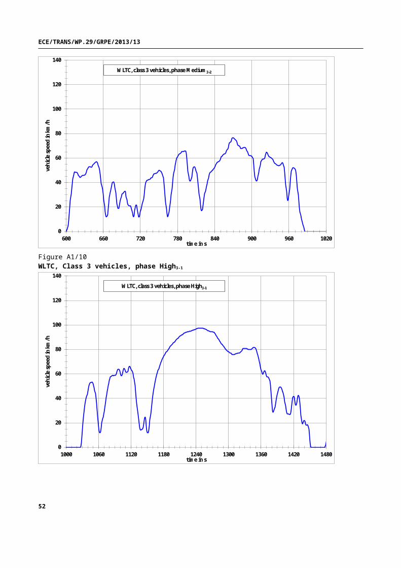
ECE/TRANS/WP.29/GRPE/2013/13
Time in s speed in km/h Time in s speed in km/h Time in s speed in km/h Time in s speed in km/h
974 31.7975 27976 24.7977 19.3978 16979 13.2980 10.7981 8.8982 7.2983 5.5984 3.2985 1.1986 0987 0988 0989 0990 0991 0992 0993 0994 0995 0996 0997 0998 0999 0
1000 01001 01002 01003 01004 01005 01006 01007 01008 01009 01010 01011 01012 01013 01014 01015 01016 01017 01018 01019 01020 01021 01022 0
52

ECE/TRANS/WP.29/GRPE/2013/13
Table A1/9WLTC, Class 3 vehicles, phase Medium3-2
Time in s speed in km/h Time in s speed in km/h Time in s speed in km/h Time in s speed in km/h
590 0 637 53 684 18.9 731 41.9591 0 638 53 685 18.9 732 42592 0 639 52.9 686 21.3 733 42.2593 0 640 52.7 687 23.9 734 42.4594 0 641 52.6 688 25.9 735 42.7595 0 642 53.1 689 28.4 736 43.1596 0 643 54.3 690 30.3 737 43.7597 0 644 55.2 691 30.9 738 44598 0 645 55.5 692 31.1 739 44.1599 0 646 55.9 693 31.8 740 45.3600 0 647 56.3 694 32.7 741 46.4601 1 648 56.7 695 33.2 742 47.2602 2.1 649 56.9 696 32.4 743 47.3603 4.8 650 56.8 697 28.3 744 47.4604 9.1 651 56 698 25.8 745 47.4605 14.2 652 54.2 699 23.1 746 47.5606 19.8 653 52.1 700 21.8 747 47.9607 25.5 654 50.1 701 21.2 748 48.6608 30.5 655 47.2 702 21 749 49.4609 34.8 656 43.2 703 21 750 49.8610 38.8 657 39.2 704 20.9 751 49.8611 42.9 658 36.5 705 19.9 752 49.7612 46.4 659 34.3 706 17.9 753 49.3613 48.3 660 31 707 15.1 754 48.5614 48.7 661 26 708 12.8 755 47.6615 48.5 662 20.7 709 12 756 46.3616 48.4 663 15.4 710 13.2 757 43.7617 48.2 664 13.1 711 17.1 758 39.3618 47.8 665 12 712 21.1 759 34.1619 47 666 12.5 713 21.8 760 29620 45.9 667 14 714 21.2 761 23.7621 44.9 668 19 715 18.5 762 18.4622 44.4 669 23.2 716 13.9 763 14.3623 44.3 670 28 717 12 764 12624 44.5 671 32 718 12 765 12.8625 45.1 672 34 719 13 766 16626 45.7 673 36 720 16 767 19.1627 46 674 38 721 18.5 768 22.4628 46 675 40 722 20.6 769 25.6629 46 676 40.3 723 22.5 770 30.1630 46.1 677 40.5 724 24 771 35.3631 46.7 678 39 725 26.6 772 39.9632 47.7 679 35.7 726 29.9 773 44.5633 48.9 680 31.8 727 34.8 774 47.5634 50.3 681 27.1 728 37.8 775 50.9635 51.6 682 22.8 729 40.2 776 54.1636 52.6 683 21.1 730 41.6 777 56.3
53

ECE/TRANS/WP.29/GRPE/2013/13
Time in s speed in km/h Time in s speed in km/h Time in s speed in km/h Time in s speed in km/h
778 58.1 827 37.1 876 72.7 925 64.1779 59.8 828 38.9 877 71.3 926 62.7780 61.1 829 41.4 878 70.4 927 62781 62.1 830 44 879 70 928 61.3782 62.8 831 46.3 880 70 929 60.9783 63.3 832 47.7 881 69 930 60.5784 63.6 833 48.2 882 68 931 60.2785 64 834 48.7 883 68 932 59.8786 64.7 835 49.3 884 68 933 59.4787 65.2 836 49.8 885 68.1 934 58.6788 65.3 837 50.2 886 68.4 935 57.5789 65.3 838 50.9 887 68.6 936 56.6790 65.4 839 51.8 888 68.7 937 56791 65.7 840 52.5 889 68.5 938 55.5792 66 841 53.3 890 68.1 939 55793 65.6 842 54.5 891 67.3 940 54.4794 63.5 843 55.7 892 66.2 941 54.1795 59.7 844 56.5 893 64.8 942 54796 54.6 845 56.8 894 63.6 943 53.9797 49.3 846 57 895 62.6 944 53.9798 44.9 847 57.2 896 62.1 945 54799 42.3 848 57.7 897 61.9 946 54.2800 41.4 849 58.7 898 61.9 947 55801 41.3 850 60.1 899 61.8 948 55.8802 42.1 851 61.1 900 61.5 949 56.2803 44.7 852 61.7 901 60.9 950 56.1804 48.4 853 62.3 902 59.7 951 55.1805 51.4 854 62.9 903 54.6 952 52.7806 52.7 855 63.3 904 49.3 953 48.4807 53 856 63.4 905 44.9 954 43.1808 52.5 857 63.5 906 42.3 955 37.8809 51.3 858 64.5 907 41.4 956 32.5810 49.7 859 65.8 908 41.3 957 27.2811 47.4 860 66.8 909 42.1 958 25.1812 43.7 861 67.4 910 44.7 959 26813 39.7 862 68.8 911 48.4 960 29.3814 35.5 863 71.1 912 51.4 961 34.6815 31.1 864 72.3 913 52.7 962 40.4816 26.3 865 72.8 914 54 963 45.3817 21.9 866 73.4 915 57 964 49818 18 867 74.6 916 58.1 965 51.1819 17 868 76 917 59.2 966 52.1820 18 869 76.6 918 59 967 52.2821 21.4 870 76.5 919 59.1 968 52.1822 24.8 871 76.2 920 59.5 969 51.7823 27.9 872 75.8 921 60.5 970 50.9824 30.8 873 75.4 922 62.3 971 49.2825 33 874 74.8 923 63.9 972 45.9826 35.1 875 73.9 924 65.1 973 40.6
54

ECE/TRANS/WP.29/GRPE/2013/13
Time in s speed in km/h Time in s speed in km/h Time in s speed in km/h Time in s speed in km/h
974 35.3975 30976 24.7977 19.3978 16979 13.2980 10.7981 8.8982 7.2983 5.5984 3.2985 1.1986 0987 0988 0989 0990 0991 0992 0993 0994 0995 0996 0997 0998 0999 0
1000 01001 01002 01003 01004 01005 01006 01007 01008 01009 01010 01011 01012 01013 01014 01015 01016 01017 01018 01019 01020 01021 01022 0
55

ECE/TRANS/WP.29/GRPE/2013/13
Table A1/10WLTC, Class 3 vehicles, phase High3-1
Time in s speed in km/h Time in s speed in km/h Time in s speed in km/h Time in s speed in km/h
1023 0 1070 29 1117 66.2 1164 52.61024 0 1071 32 1118 65.8 1165 54.51025 0 1072 34.8 1119 64.7 1166 56.61026 0 1073 37.7 1120 63.6 1167 58.31027 0.8 1074 40.8 1121 62.9 1168 601028 3.6 1075 43.2 1122 62.4 1169 61.51029 8.6 1076 46 1123 61.7 1170 63.11030 14.6 1077 48 1124 60.1 1171 64.31031 20 1078 50.7 1125 57.3 1172 65.71032 24.4 1079 52 1126 55.8 1173 67.11033 28.2 1080 54.5 1127 50.5 1174 68.31034 31.7 1081 55.9 1128 45.2 1175 69.71035 35 1082 57.4 1129 40.1 1176 70.61036 37.6 1083 58.1 1130 36.2 1177 71.61037 39.7 1084 58.4 1131 32.9 1178 72.61038 41.5 1085 58.8 1132 29.8 1179 73.51039 43.6 1086 58.8 1133 26.6 1180 74.21040 46 1087 58.6 1134 23 1181 74.91041 48.4 1088 58.7 1135 19.4 1182 75.61042 50.5 1089 58.8 1136 16.3 1183 76.31043 51.9 1090 58.8 1137 14.6 1184 77.11044 52.6 1091 58.8 1138 14.2 1185 77.91045 52.8 1092 59.1 1139 14.3 1186 78.51046 52.9 1093 60.1 1140 14.6 1187 791047 53.1 1094 61.7 1141 15.1 1188 79.71048 53.3 1095 63 1142 16.4 1189 80.31049 53.1 1096 63.7 1143 19.1 1190 811050 52.3 1097 63.9 1144 22.5 1191 81.61051 50.7 1098 63.5 1145 24.4 1192 82.41052 48.8 1099 62.3 1146 24.8 1193 82.91053 46.5 1100 60.3 1147 22.7 1194 83.41054 43.8 1101 58.9 1148 17.4 1195 83.81055 40.3 1102 58.4 1149 13.8 1196 84.21056 36 1103 58.8 1150 12 1197 84.71057 30.7 1104 60.2 1151 12 1198 85.21058 25.4 1105 62.3 1152 12 1199 85.61059 21 1106 63.9 1153 13.9 1200 86.31060 16.7 1107 64.5 1154 17.7 1201 86.81061 13.4 1108 64.4 1155 22.8 1202 87.41062 12 1109 63.5 1156 27.3 1203 881063 12.1 1110 62 1157 31.2 1204 88.31064 12.8 1111 61.2 1158 35.2 1205 88.71065 15.6 1112 61.3 1159 39.4 1206 891066 19.9 1113 61.7 1160 42.5 1207 89.31067 23.4 1114 62 1161 45.4 1208 89.81068 24.6 1115 64.6 1162 48.2 1209 90.21069 27 1116 66 1163 50.3 1210 90.6
56

ECE/TRANS/WP.29/GRPE/2013/13
Time in s speed in km/h Time in s speed in km/h Time in s speed in km/h Time in s speed in km/h
1211 91 1260 95.7 1309 75.9 1358 68.21212 91.3 1261 95.5 1310 76 1359 66.11213 91.6 1262 95.3 1311 76 1360 63.81214 91.9 1263 95.2 1312 76.1 1361 61.61215 92.2 1264 95 1313 76.3 1362 60.21216 92.8 1265 94.9 1314 76.5 1363 59.81217 93.1 1266 94.7 1315 76.6 1364 60.41218 93.3 1267 94.5 1316 76.8 1365 61.81219 93.5 1268 94.4 1317 77.1 1366 62.61220 93.7 1269 94.4 1318 77.1 1367 62.71221 93.9 1270 94.3 1319 77.2 1368 61.91222 94 1271 94.3 1320 77.2 1369 601223 94.1 1272 94.1 1321 77.6 1370 58.41224 94.3 1273 93.9 1322 78 1371 57.81225 94.4 1274 93.4 1323 78.4 1372 57.81226 94.6 1275 92.8 1324 78.8 1373 57.81227 94.7 1276 92 1325 79.2 1374 57.31228 94.8 1277 91.3 1326 80.3 1375 56.21229 95 1278 90.6 1327 80.8 1376 54.31230 95.1 1279 90 1328 81 1377 50.81231 95.3 1280 89.3 1329 81 1378 45.51232 95.4 1281 88.7 1330 81 1379 40.21233 95.6 1282 88.1 1331 81 1380 34.91234 95.7 1283 87.4 1332 81 1381 29.61235 95.8 1284 86.7 1333 80.9 1382 28.71236 96 1285 86 1334 80.6 1383 29.31237 96.1 1286 85.3 1335 80.3 1384 30.51238 96.3 1287 84.7 1336 80 1385 31.71239 96.4 1288 84.1 1337 79.9 1386 32.91240 96.6 1289 83.5 1338 79.8 1387 351241 96.8 1290 82.9 1339 79.8 1388 381242 97 1291 82.3 1340 79.8 1389 40.51243 97.2 1292 81.7 1341 79.9 1390 42.71244 97.3 1293 81.1 1342 80 1391 45.81245 97.4 1294 80.5 1343 80.4 1392 47.51246 97.4 1295 79.9 1344 80.8 1393 48.91247 97.4 1296 79.4 1345 81.2 1394 49.41248 97.4 1297 79.1 1346 81.5 1395 49.41249 97.3 1298 78.8 1347 81.6 1396 49.21250 97.3 1299 78.5 1348 81.6 1397 48.71251 97.3 1300 78.2 1349 81.4 1398 47.91252 97.3 1301 77.9 1350 80.7 1399 46.91253 97.2 1302 77.6 1351 79.6 1400 45.61254 97.1 1303 77.3 1352 78.2 1401 44.21255 97 1304 77 1353 76.8 1402 42.71256 96.9 1305 76.7 1354 75.3 1403 40.71257 96.7 1306 76 1355 73.8 1404 37.11258 96.4 1307 76 1356 72.1 1405 33.91259 96.1 1308 76 1357 70.2 1406 30.6
57

ECE/TRANS/WP.29/GRPE/2013/13
Time in s speed in km/h Time in s speed in km/h Time in s speed in km/h Time in s speed in km/h
1407 28.6 1456 01408 27.3 1457 01409 27.2 1458 01410 27.5 1459 01411 27.4 1460 01412 27.1 1461 01413 26.7 1462 01414 26.8 1463 01415 28.2 1464 01416 31.1 1465 01417 34.8 1466 01418 38.4 1467 01419 40.9 1468 01420 41.7 1469 01421 40.9 1470 01422 38.3 1471 01423 35.3 1472 01424 34.3 1473 01425 34.6 1474 01426 36.3 1475 01427 39.5 1476 01428 41.8 1477 01429 42.51430 41.91431 40.11432 36.61433 31.31434 261435 20.61436 19.11437 19.71438 21.11439 221440 22.11441 21.41442 19.61443 18.31444 181445 18.31446 18.51447 17.91448 151449 9.91450 4.61451 1.21452 01453 01454 01455 0
58

ECE/TRANS/WP.29/GRPE/2013/13
Table A1/11WLTC, Class 3 vehicles, phase High3-2
Time in s speed in km/h Time in s speed in km/h Time in s speed in km/h Time in s speed in km/h
1023 0 1070 26.4 1117 69.7 1164 52.61024 0 1071 28.8 1118 69.3 1165 54.51025 0 1072 31.8 1119 68.1 1166 56.61026 0 1073 35.3 1120 66.9 1167 58.31027 0.8 1074 39.5 1121 66.2 1168 601028 3.6 1075 44.5 1122 65.7 1169 61.51029 8.6 1076 49.3 1123 64.9 1170 63.11030 14.6 1077 53.3 1124 63.2 1171 64.31031 20 1078 56.4 1125 60.3 1172 65.71032 24.4 1079 58.9 1126 55.8 1173 67.11033 28.2 1080 61.2 1127 50.5 1174 68.31034 31.7 1081 62.6 1128 45.2 1175 69.71035 35 1082 63 1129 40.1 1176 70.61036 37.6 1083 62.5 1130 36.2 1177 71.61037 39.7 1084 60.9 1131 32.9 1178 72.61038 41.5 1085 59.3 1132 29.8 1179 73.51039 43.6 1086 58.6 1133 26.6 1180 74.21040 46 1087 58.6 1134 23 1181 74.91041 48.4 1088 58.7 1135 19.4 1182 75.61042 50.5 1089 58.8 1136 16.3 1183 76.31043 51.9 1090 58.8 1137 14.6 1184 77.11044 52.6 1091 58.8 1138 14.2 1185 77.91045 52.8 1092 59.1 1139 14.3 1186 78.51046 52.9 1093 60.1 1140 14.6 1187 791047 53.1 1094 61.7 1141 15.1 1188 79.71048 53.3 1095 63 1142 16.4 1189 80.31049 53.1 1096 63.7 1143 19.1 1190 811050 52.3 1097 63.9 1144 22.5 1191 81.61051 50.7 1098 63.5 1145 24.4 1192 82.41052 48.8 1099 62.3 1146 24.8 1193 82.91053 46.5 1100 60.3 1147 22.7 1194 83.41054 43.8 1101 58.9 1148 17.4 1195 83.81055 40.3 1102 58.4 1149 13.8 1196 84.21056 36 1103 58.8 1150 12 1197 84.71057 30.7 1104 60.2 1151 12 1198 85.21058 25.4 1105 62.3 1152 12 1199 85.61059 21 1106 63.9 1153 13.9 1200 86.31060 16.7 1107 64.5 1154 17.7 1201 86.81061 13.4 1108 64.4 1155 22.8 1202 87.41062 12 1109 63.5 1156 27.3 1203 881063 12.1 1110 62 1157 31.2 1204 88.31064 12.8 1111 61.2 1158 35.2 1205 88.71065 15.6 1112 61.3 1159 39.4 1206 891066 19.9 1113 62.6 1160 42.5 1207 89.31067 23.4 1114 65.3 1161 45.4 1208 89.81068 24.6 1115 68 1162 48.2 1209 90.21069 25.2 1116 69.4 1163 50.3 1210 90.6
59

ECE/TRANS/WP.29/GRPE/2013/13
Time in s speed in km/h Time in s speed in km/h Time in s speed in km/h Time in s speed in km/h
1211 91 1260 95.7 1309 75.9 1358 68.21212 91.3 1261 95.5 1310 75.9 1359 66.11213 91.6 1262 95.3 1311 75.8 1360 63.81214 91.9 1263 95.2 1312 75.7 1361 61.61215 92.2 1264 95 1313 75.5 1362 60.21216 92.8 1265 94.9 1314 75.2 1363 59.81217 93.1 1266 94.7 1315 75 1364 60.41218 93.3 1267 94.5 1316 74.7 1365 61.81219 93.5 1268 94.4 1317 74.1 1366 62.61220 93.7 1269 94.4 1318 73.7 1367 62.71221 93.9 1270 94.3 1319 73.3 1368 61.91222 94 1271 94.3 1320 73.5 1369 601223 94.1 1272 94.1 1321 74 1370 58.41224 94.3 1273 93.9 1322 74.9 1371 57.81225 94.4 1274 93.4 1323 76.1 1372 57.81226 94.6 1275 92.8 1324 77.7 1373 57.81227 94.7 1276 92 1325 79.2 1374 57.31228 94.8 1277 91.3 1326 80.3 1375 56.21229 95 1278 90.6 1327 80.8 1376 54.31230 95.1 1279 90 1328 81 1377 50.81231 95.3 1280 89.3 1329 81 1378 45.51232 95.4 1281 88.7 1330 81 1379 40.21233 95.6 1282 88.1 1331 81 1380 34.91234 95.7 1283 87.4 1332 81 1381 29.61235 95.8 1284 86.7 1333 80.9 1382 27.31236 96 1285 86 1334 80.6 1383 29.31237 96.1 1286 85.3 1335 80.3 1384 32.91238 96.3 1287 84.7 1336 80 1385 35.61239 96.4 1288 84.1 1337 79.9 1386 36.71240 96.6 1289 83.5 1338 79.8 1387 37.61241 96.8 1290 82.9 1339 79.8 1388 39.41242 97 1291 82.3 1340 79.8 1389 42.51243 97.2 1292 81.7 1341 79.9 1390 46.51244 97.3 1293 81.1 1342 80 1391 50.21245 97.4 1294 80.5 1343 80.4 1392 52.81246 97.4 1295 79.9 1344 80.8 1393 54.31247 97.4 1296 79.4 1345 81.2 1394 54.91248 97.4 1297 79.1 1346 81.5 1395 54.91249 97.3 1298 78.8 1347 81.6 1396 54.71250 97.3 1299 78.5 1348 81.6 1397 54.11251 97.3 1300 78.2 1349 81.4 1398 53.21252 97.3 1301 77.9 1350 80.7 1399 52.11253 97.2 1302 77.6 1351 79.6 1400 50.71254 97.1 1303 77.3 1352 78.2 1401 49.11255 97 1304 77 1353 76.8 1402 47.41256 96.9 1305 76.7 1354 75.3 1403 45.21257 96.7 1306 76 1355 73.8 1404 41.81258 96.4 1307 76 1356 72.1 1405 36.51259 96.1 1308 76 1357 70.2 1406 31.2
60

ECE/TRANS/WP.29/GRPE/2013/13
Time in s speed in km/h Time in s speed in km/h Time in s speed in km/h Time in s speed in km/h
1407 27.6 1456 01408 26.9 1457 01409 27.3 1458 01410 27.5 1459 01411 27.4 1460 01412 27.1 1461 01413 26.7 1462 01414 26.8 1463 01415 28.2 1464 01416 31.1 1465 01417 34.8 1466 01418 38.4 1467 01419 40.9 1468 01420 41.7 1469 01421 40.9 1470 01422 38.3 1471 01423 35.3 1472 01424 34.3 1473 01425 34.6 1474 01426 36.3 1475 01427 39.5 1476 01428 41.8 1477 01429 42.51430 41.91431 40.11432 36.61433 31.31434 261435 20.61436 19.11437 19.71438 21.11439 221440 22.11441 21.41442 19.61443 18.31444 181445 18.31446 18.51447 17.91448 151449 9.91450 4.61451 1.21452 01453 01454 01455 0
61

ECE/TRANS/WP.29/GRPE/2013/13
Table A1/12WLTC, Class 3 vehicles, phase Extra High3
Time in s speed in km/h Time in s speed in km/h Time in s speed in km/h Time in s speed in km/h
1478 0 1525 72.5 1572 120.7 1619 1131479 2.2 1526 70.8 1573 121.8 1620 114.11480 4.4 1527 68.6 1574 122.6 1621 115.11481 6.3 1528 66.2 1575 123.2 1622 115.91482 7.9 1529 64 1576 123.6 1623 116.51483 9.2 1530 62.2 1577 123.7 1624 116.71484 10.4 1531 60.9 1578 123.6 1625 116.61485 11.5 1532 60.2 1579 123.3 1626 116.21486 12.9 1533 60 1580 123 1627 115.21487 14.7 1534 60.4 1581 122.5 1628 113.81488 17 1535 61.4 1582 122.1 1629 1121489 19.8 1536 63.2 1583 121.5 1630 110.11490 23.1 1537 65.6 1584 120.8 1631 108.31491 26.7 1538 68.4 1585 120 1632 1071492 30.5 1539 71.6 1586 119.1 1633 106.11493 34.1 1540 74.9 1587 118.1 1634 105.81494 37.5 1541 78.4 1588 117.1 1635 105.71495 40.6 1542 81.8 1589 116.2 1636 105.71496 43.3 1543 84.9 1590 115.5 1637 105.61497 45.7 1544 87.4 1591 114.9 1638 105.31498 47.7 1545 89 1592 114.5 1639 104.91499 49.3 1546 90 1593 114.1 1640 104.41500 50.5 1547 90.6 1594 113.9 1641 1041501 51.3 1548 91 1595 113.7 1642 103.81502 52.1 1549 91.5 1596 113.3 1643 103.91503 52.7 1550 92 1597 112.9 1644 104.41504 53.4 1551 92.7 1598 112.2 1645 105.11505 54 1552 93.4 1599 111.4 1646 106.11506 54.5 1553 94.2 1600 110.5 1647 107.21507 55 1554 94.9 1601 109.5 1648 108.51508 55.6 1555 95.7 1602 108.5 1649 109.91509 56.3 1556 96.6 1603 107.7 1650 111.31510 57.2 1557 97.7 1604 107.1 1651 112.71511 58.5 1558 98.9 1605 106.6 1652 113.91512 60.2 1559 100.4 1606 106.4 1653 1151513 62.3 1560 102 1607 106.2 1654 1161514 64.7 1561 103.6 1608 106.2 1655 116.81515 67.1 1562 105.2 1609 106.2 1656 117.61516 69.2 1563 106.8 1610 106.4 1657 118.41517 70.7 1564 108.5 1611 106.5 1658 119.21518 71.9 1565 110.2 1612 106.8 1659 1201519 72.7 1566 111.9 1613 107.2 1660 120.81520 73.4 1567 113.7 1614 107.8 1661 121.61521 73.8 1568 115.3 1615 108.5 1662 122.31522 74.1 1569 116.8 1616 109.4 1663 123.11523 74 1570 118.2 1617 110.5 1664 123.81524 73.6 1571 119.5 1618 111.7 1665 124.4
62

ECE/TRANS/WP.29/GRPE/2013/13
Time in s speed in km/h Time in s speed in km/h Time in s speed in km/h Time in s speed in km/h
1666 125 1715 127.7 1764 821667 125.4 1716 128.1 1765 81.31668 125.8 1717 128.5 1766 80.41669 126.1 1718 129 1767 79.11670 126.4 1719 129.5 1768 77.41671 126.6 1720 130.1 1769 75.11672 126.7 1721 130.6 1770 72.31673 126.8 1722 131 1771 69.11674 126.9 1723 131.2 1772 65.91675 126.9 1724 131.3 1773 62.71676 126.9 1725 131.2 1774 59.71677 126.8 1726 130.7 1775 571678 126.6 1727 129.8 1776 54.61679 126.3 1728 128.4 1777 52.21680 126 1729 126.5 1778 49.71681 125.7 1730 124.1 1779 46.81682 125.6 1731 121.6 1780 43.51683 125.6 1732 119 1781 39.91684 125.8 1733 116.5 1782 36.41685 126.2 1734 114.1 1783 33.21686 126.6 1735 111.8 1784 30.51687 127 1736 109.5 1785 28.31688 127.4 1737 107.1 1786 26.31689 127.6 1738 104.8 1787 24.41690 127.8 1739 102.5 1788 22.51691 127.9 1740 100.4 1789 20.51692 128 1741 98.6 1790 18.21693 128.1 1742 97.2 1791 15.51694 128.2 1743 95.9 1792 12.31695 128.3 1744 94.8 1793 8.71696 128.4 1745 93.8 1794 5.21697 128.5 1746 92.8 1795 01698 128.6 1747 91.8 1796 01699 128.6 1748 91 1797 01700 128.5 1749 90.2 1798 01701 128.3 1750 89.6 1799 01702 128.1 1751 89.1 1800 01703 127.9 1752 88.61704 127.6 1753 88.11705 127.4 1754 87.61706 127.2 1755 87.11707 127 1756 86.61708 126.9 1757 86.11709 126.8 1758 85.51710 126.7 1759 851711 126.8 1760 84.41712 126.9 1761 83.81713 127.1 1762 83.21714 127.4 1763 82.6
63

ECE/TRANS/WP.29/GRPE/2013/13
7. Cycle modification
7.1. General remarks
The cycle to be driven shall depend on the test vehicle’s rated power to unladen mass ratio, W/kg, and its maximum velocity, vmax.
Driveability problems may occur for vehicles with power to mass ratios close to the borderlines between Class 2 and Class 3 vehicles or very low powered vehicles in Class 1.
Since these problems are related mainly to cycle phases with a combination of high vehicle speed and high accelerations rather than to the maximum speed of the cycle, the downscaling procedure shall be applied to improve driveability.
This section shall not apply to vehicles tested according to Annex 8.
7.2. This section describes the method to modify the cycle profile using the downscaling procedure.
7.2.1. Downscaling procedure for class 1 vehicles
Figure A1/13Downscaled medium speed phase of the class 1 WLTC
0
10
20
30
40
50
60
70
590 650 710 770 830 890 950 1010
vehi
cle
spee
d in
km
/h
time in s
WLTC class 1, phase Medium1
v_downscaled
Downscaling example, DSC_factor = 0.25
For the class 1 cycle, the downscaling period is the time period between second 651 and second 906. Within this time period, the acceleration for the original cycle shall be calculated using the following equation:
aorigi=
v i+1−v i
3.6(1)
where:
64

ECE/TRANS/WP.29/GRPE/2013/13
vi is the vehicle speed, km/h;
i is the time between 651 and 906 s.
The downscaling shall be first applied in the time period between second 651 and 848. The downscaled speed trace shall then be calculated using the following equation:
vdsc i+1=vdsci
+aorigi× (1−dscfactor )× 3.6 (2)
with i=651¿847
For i=651, vdsci=v origi
.
In order to meet the original vehicle speed at second 907, a correction factor for the deceleration shall be calculated using the following equation:
f corrdec=
vdsc¿
vorig¿
(3)
where 36.7 km/h is the original vehicle speed at second 907.
The downscaled vehicle speed between 849 and 906 s shall then be calculated using the following equation:
vdsci=v dsci−1
+aorigi−1× f corrdec
×3.6 (4)
With i=849 ¿906.
7.2.2. Downscaling procedure for class 2 vehicles
Since the driveability problems are exclusively related to the extra high speed phases of the class 2 and class 3 cycles, the downscaling is related to those sections of the extra high speed phases where the driveability problems occur (see Figure A1/14).
Figure A1/14Downscaled extra high speed phase of the class 2 WLTC
65

ECE/TRANS/WP.29/GRPE/2013/13
0
20
40
60
80
100
120
140
1440 1500 1560 1620 1680 1740 1800
vehi
cle
spee
d in
km
/h
time in s
WLTC, class 2, phase Extra High2
v_downscaled
For the class 2 cycle, the downscaling period is the time period between second 1520 and second 1742. Within this time period, the acceleration for the original cycle shall be calculated using the following equation:
aorigi=
v i+1−v i
3.6(5)
where:
vi is the vehicle speed, km/h;
i is the time between 1520 and 1742 s.
The downscaling shall be applied first in the time period between second 1520 and 1725. Second 1725 is the time where the maximum speed of the extra high speed phase is reached. The downscaled speed trace shall then be calculated using the following equation:
vdsci+1=vdsci
+aorigi× (1−dsc factor ) ×3.6 (6)
with i=1520 ¿1725.
For i=1520, vdsci=v origi
.
In order to meet the original vehicle speed at second 1743, a correction factor for the deceleration shall be calculated using the following equation:
f corrdec=
vdsc¿
vorig¿
(7)
90.4 km/h is the original vehicle speed at second 1743.
66

ECE/TRANS/WP.29/GRPE/2013/13
The downscaled vehicle speed between 1726 and 1742 s shall be calculated using the following equation:
vdsci=v dsci−1
+aorigi−1× f corrdec
×3.6 (8)
with i=1726 ¿1742.
7.2.3. Downscaling procedure for class 3 vehicles
Figure A1/15 shows an example for a downscaled extra high speed phase of the class 3 WLTC.
Figure A1/15Downscaled extra high speed phase of the class 3 WLTC
0
20
40
60
80
100
120
140
1440 1500 1560 1620 1680 1740 1800
vehi
cle
spee
d in
km
/h
time in s
WLTC class 3, phase Extra High3
v_downscaled
For the class 3 cycle, this is the period between second 1533 and second 1762. Within this time period the acceleration for the original cycle shall be calculated using the following equation:
aorigi=
v i+1−v i
3.6(9)
where:
vi is the vehicle speed, km/h;
i is the time between 1533 and 1762 s.
The downscaling shall be applied first in the time period between second 1533 and 1724. Second 1724 is the time where the maximum speed of the extra high speed phase is reached. The downscaled speed trace shall then be calculated using the following equation:
vdsci+1=vdsci
+aorigi× (1−dsc factor ) ×3.6 (10)
67

ECE/TRANS/WP.29/GRPE/2013/13
with i=1533 ¿1723.
For i=1533, vdsci=v origi
.
In order to meet the original vehicle speed at second 1763, a correction factor for the deceleration is calculated using the following equation:
f corrdec=
vdsc¿
vorig¿
(11)
82.6 km/h is the original vehicle speed at second 1763.
The downscaled vehicle speed between 1725 and 1762 s shall then be calculated using the following equation:
vdsci=v dsci−1
+aorigi−1× f corrdec
×3.6 (12)
with i=1725 ¿1762.
7.3. Determination of the downscaling factor
The downscaling factor f dsc is a function of the ratio, rmax, between the maximum required power of the cycle phases where the downscaling is to be applied and the rated power of the vehicle (Prated).
The maximum required power, Preq ,max ,i in kW, is related to a specific time i in the cycle trace and is calculated from the driving resistance coefficients f 0, f1, f2 and the test mass TM as follows:
Preq ,max ,i=( (f 0× v i )+( f 1× v i
2 )+( f 2× v i3 )+(1.1 ×TM × v i ×a i) )
3600(13)
with f 0 in N, f 1 in N/(km/h) and f 2 in N/(km/h)2, TM in kg.
The cycle time i, at which maximum power or power values close to maximum power is required, is: 764 s for class 1, 1574 s for class 2 and 1566 s for class 3.
The corresponding vehicle speed values vi and acceleration values a i are as follows:
vi=61.4 km/h, a i=0.22 m/s² for class 1,
vi=109.9 km/h, a i=0.36 m/s² for class 2,
vi=111.9 km/h, a i=0.50 m/s² for class 3.
The driving resistance coefficients f 0, f 1 and f 2 shall be determined by coastdown measurements or an equivalent method.
rmax is calculated using the following equation:
rmax=Preq ,max, i
Prated(14)
The downscaling factor f dsc is calculated using the following equations:
if rmax <r0, then f dsc=0
68

ECE/TRANS/WP.29/GRPE/2013/13
if rmax ≥ r0, then f dsc=a1× rmax+b1 (15)
The calculation parameter/coefficients r0, a1 and b1 are as follows:
Class 1 r0=1.0, a1=0.54, b1=−0.54
Class 2 for vehicles with vmax>105 km/h, r0=1.0, a1=0.6, b1=−0.6. No downscaling shall be applied for vehicles with vmax ≤105 km/h
Class 3 for vehicles with vmax>112 km/h, r0=1.0, a1=0.65, b1=−0.65; for vehicles with vmax ≤112 km/h, r0=1.3, a1=0.65, b1=−0.65.
The resulting f dsc is mathematically rounded to one digit behind the comma and is only applied if it exceeds one per cent.
7.4. Additional requirements
If a vehicle is tested under different configurations in terms of test mass and driving resistance coefficients, vehicle L as defined in section 4.2.1. of Annex 4 shall be used for the determination of the downscaling factor and the resulting downscaled cycle shall be used for all measurements.
If the maximum speed of the vehicle is lower than the maximum speed of the downscaled cycle, the vehicle shall be driven with its maximum speed in those cycle periods where the cycle speed is higher than the maximum speed of the vehicle.
If the vehicle cannot follow the speed trace of the downscaled cycle within the tolerance for specific periods, it shall be driven with the accelerator control fully activated during these periods. During such periods of operation, driving trace violations shall be ignored.
69

ECE/TRANS/WP.29/GRPE/2013/13
Annex 2
Gear selection and shift point determination for vehicles equipped with manual transmissions
1. General approach
1.1. The shifting procedures described in this Annex shall apply to vehicles equipped with manual and semi-automatic transmissions.
1.2. The prescribed gears and shifting points are based on the balance between the power required to overcome driving resistance and acceleration, and the power provided by the engine in all possible gears at a specific cycle phase.
1.3. The calculation to determine the gears to use shall be based on normalised engine speeds (normalised to the span between idling speed and rated engine speed) and normalised full load power curves (normalised to rated power) versus normalised engine speed.
1.4. This annex shall not apply to vehicles tested according to Annex 8..
2. Required data
The following data is required to calculate the gears to be used when driving the cycle on a chassis dynamometer:
(a) Prated , the maximum rated engine power as declared by the manufacturer;
(b) s, the rated engine speed at which an engine develops its maximum power. If the maximum power is developed over an engine speed range, s is determined by the mean of this range;
(c) nidle, idling speed as defined of Annex 1;
(d) ngmax, the number of forward gears;
(e) nmin drive, minimum engine speed for gears i>2 when the vehicle is in
motion. The minimum value is determined by the following equation:
nmindrive=nidle+0.125 × (s−n idle) (1)
Higher values may be used if requested by the manufacturer;
(f) ndv i, the ratio obtained by dividing n in min-1 by v in km/h for each gear i, i=1 to ngmax;
(g) TM , test mass of the vehicle in kg;
(h) f 0, f 1, f 2, driving resistance coefficients as defined of Annex 4 in N, N/(km/h), and N/(km/h)² respectively;
70

ECE/TRANS/WP.29/GRPE/2013/13
(i)Pwot(nnorm)
Prated is the full load power curve, normalised to rated power
and (rated engine speed – idling speed), where nnorm=n−nidle
s−nidle.
3. Calculations of required power, engine speeds, available power, and possible gear to be used
3.1. Calculation of required power
For every second j of the cycle trace, the power required to overcome driving resistance and to accelerate shall be calculated using the following equation:
Prequired , j=( f 0 × v j+f 1 × v j2+ f 2 × v j
3
3600 )+ kr × a j× v j ×TM3600
(2)
where:
f 0 is the road load coefficient, N;
f 1 is the road load parameter dependent on velocity, N/(km/h);
f 2 is the road load parameter based on the square of velocity, N/(km/h)²;
Prequired , j is the required power in kW at second j;
v j is the vehicle speed at second j, km/h;
a j is the vehicle acceleration at second j, m/s²,
a j=(v j+1−v j)
3.6;
TM is the vehicle test mass, kg;
kr is a factor taking the inertial resistances of the drivetrain during acceleration into account and is set to 1.1.
3.2. Determination of engine speeds
For each v j≤ 1 km/h, the engine speed is set to nidle and the gear lever is placed in neutral with the clutch engaged.
For each v j≥ 1 km/h of the cycle trace and each gear i, i=1 to ngmax, the engine speed ni , j is calculated using the following equation:
ni , j=ndvi × v j (3)
All gears i for which nmin ≤ni , j ≤ nmax are possible gears to be used for driving the cycle trace at v j.
ifi>2,
nmax=1.2 × ( s−nidle )+nidle
nmin=nmindrive;
71

ECE/TRANS/WP.29/GRPE/2013/13
if i=2 and ndv2 ×v j≥ 0.9 ×n idle,
nmin=max (1.15× nidle ,0.03 × (s−n idle)+nidle);
if ndv2 ×v j<max (1.15 ×n idle ,0.03 × ( s−nidle )+nidle ), the clutch shall be disengaged.
if i=1,
nmin=nidle .
3.3. Calculation of available power
The available power for each possible gear i and each vehicle speed value of the cycle trace vi shall be calculated using the following equation:
Pavailablei , j=Pnormwot(nnormi . j ) × P rated × SM (4)
where:
nnor mi , j=(ndv i ) × v j−nidle
s−nidle
and:
Prated is the rated power, kW;
Pnormwotis the percentage of rated power available at nnorm i . j at full load condition from the normalised full load power curve;
SM is a safety margin accounting for the difference between stationary full load condition power curve and the power available during transition conditions. SM is set to 0.9;
nidle is the idling speed, min-1;
s is the rated engine speed.
3.4. Determination of possible gears to be used
The possible gears to be used are determined by the following conditions:
(a) nmin ≤ni , j ≤ nmax;
(b) Pavailablei , j≥ Prequired , j
The initial gear to be used for each second j of the cycle trace is the highest final possible gear imax. When starting from standstill, only the first gear shall be used.
4. Additional requirements for corrections and/or modifications of gear use
The initial gear selection shall be checked and modified in order to avoid too frequent gearshifts and to ensure driveability and practicality.
Corrections and/or modifications shall be made according to the following requirements:
72

ECE/TRANS/WP.29/GRPE/2013/13
(a) First gear shall be selected one second before beginning an acceleration phase from standstill with the clutch disengaged. Vehicle speeds below 1 km/h imply that the vehicle is standing still;
(b) Gears shall not be skipped during acceleration phases. Gears used during accelerations and decelerations must be used for a period of at least three seconds (e.g. a gear sequence 1, 1, 2, 2, 3, 3, 3, 3, 3 shall be replaced by 1, 1, 1, 2, 2, 2, 3, 3, 3);
(c) Gears may be skipped during deceleration phases. For the last phase of a deceleration to a stop, the clutch may be either disengaged or the gear lever placed in neutral and the clutch left engaged;
(d) There shall be no gearshift during transition from an acceleration phase to a deceleration phase. E.g., if v j<v j+1>v j+2 and the gear for the time sequence j and j+1 is i, gear i is also kept for the time j+2, even if the initial gear for j+2 would be i+1;
(e) If a gear i is used for a time sequence of 1 to 5 s and the gear before this sequence is the same as the gear after this sequence, e.g. i−1, the gear use for this sequence shall be corrected to i−1.
Example:
(i) a gear sequence i−1, i, i−1 is replaced by i−1, i−1, i−1;
(ii) a gear sequence i−1, i, i, i−1 is replaced by i−1, i−1, i−1, i−1;
(iii) a gear sequence i−1, i, i, i, i−1 is replaced by i−1, i−1, i−1, i−1, i−1;
(iv) a gear sequence i−1, i,i, i, i, i−1 is replaced by i−1, i−1, i−1, i−1, i−1, i−1;
(v) a gear sequence i−1, i,i,i, i, i, i−1 is replaced by i−1, i−1, i−1, i−1, i−1, i−1, i−1.
For all cases (i) to (v), gmin≤ i must be fulfilled;
(f) a gear sequence i i−1, i, shall be replaced by i, i, i, if the following conditions are fulfilled:
(i) engine speed does not drop below nmin; and
(ii) the sequence does not occur more often than four times each for the low, medium and high speed cycle phases and not more than three times for the extra high speed phase.
Requirement (ii) is necessary as the available power will drop below the required power when the gear i−1, is replaced by i;
(g) If, during an acceleration phase, a lower gear is required at a higher vehicle speed for at least 2 seconds, the higher gears before shall be corrected to the lower gear.
Example: v j<v j+1<v j+2<v j+3<v j+4<v j+5<v j+6. The originally calculated gear use is 2, 3, 3, 3, 2, 2, 3. In this case the gear use will be corrected to 2, 2, 2, 2, 2, 2, 2, 3.
73
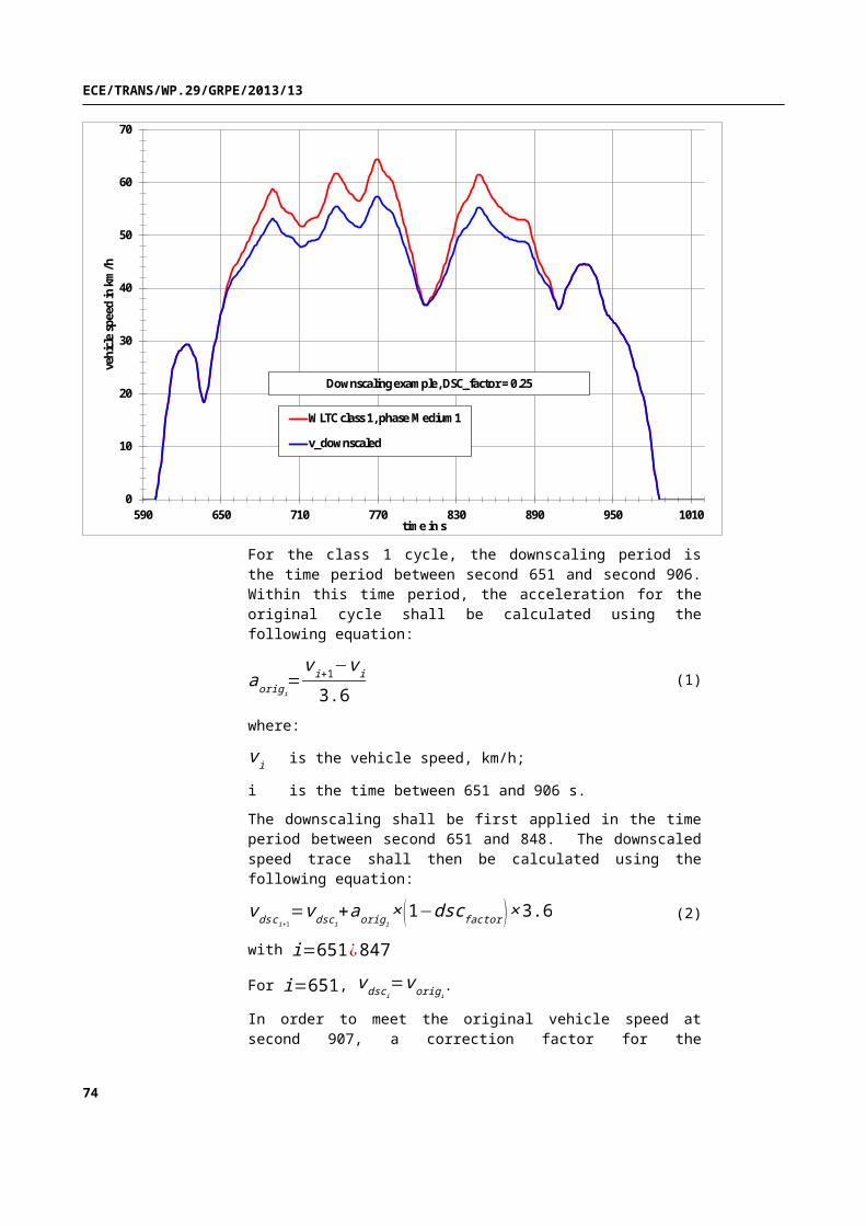
ECE/TRANS/WP.29/GRPE/2013/13
Since the above modifications may create new gear use sequences which are in conflict with these requirements, the gear sequences shall be checked twice.
74

ECE/TRANS/WP.29/GRPE/2013/13
Annex 3
Reference fuels
1. As there are regional differences in the market specifications of fuels, regionally different reference fuels need to be recognised. Example reference fuels are however required in this GTR for the calculation of hydrocarbon emissions and fuel consumption. Reference fuels are therefore given as examples for such illustrative purposes.
2. It is recommended that Contracting Parties select their reference fuels from this Annex and bring any regionally agreed amendments or alternatives into this GTR by amendment. This does not however limit the right of Contracting Parties to define individual reference fuels to reflect local market fuel specifications.
75

ECE/TRANS/WP.29/GRPE/2013/13
3. Liquid fuels for positive ignition engines
3.1. Gasoline/Petrol (nominal 90 RON, E0)
Table A3/1Gasoline/Petrol (nominal 90 RON, E0)Fuel Property or Substance Name Unit Standard Test method
Minimum MaximumResearch octane number, RON 90 92 JIS K2280Motor octane number, MON 80 82 JIS K2280Density g/cm³ 0.720 0.734 JIS K2249Vapour pressure kPa 56 60 JIS K2258Distillation:— 10 % distillation temperature K (°C) 318 (45) 328 (55) JIS K2254— 50 % distillation temperature K (°C) 363 (90) 373 (100) JIS K2254— 90 % distillation temperature K (°C) 413 (140) 443 (170) JIS K2254— final boiling point K (°C) 488 (215) JIS K2254
— olefins vol % 15 25 JIS K2536-1JIS K2536-2
— aromatics vol % 20 45JIS K2536-1JIS K2536-2JIS K2536-3
— benzene vol % 1.0JIS K2536-2JIS K2536-3JIS K2536-4
Oxygen content not to be detectedJIS K2536-2JIS K2536-4JIS K2536-6
Existent gum mg/100ml 5 JIS K2261
Sulphur content Wt ppm 10
JIS K2541-1JIS K2541-2JIS K2541-6JIS K2541-7
Lead content not to be detected JIS K2255
Ethanol not to be detectedJIS K2536-2JIS K2536-4JIS K2536-6
Methanol not to be detected
JIS K2536-2JIS K2536-4JIS K2536-5JIS K2536-6
MTBE not to be detected
JIS K2536-2JIS K2536-4JIS K2536-5JIS K2536-6
Kerosene not to be detected JIS K2536-2JIS K2536-4
76
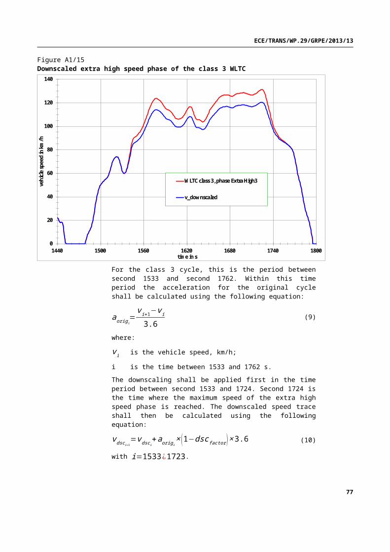
ECE/TRANS/WP.29/GRPE/2013/13
3.2. Gasoline/petrol (nominal 91 RON, E0)
Table A3/2Gasoline/petrol (nominal 91 RON, E0)Fuel Property or Substance Name
Unit Standard Test method
Minimum MaximumResearch octane number, RON 91 94 KS M 2039
Vapour pressure kPa Summer 44 60 KS M ISO 3007Winter 44 96Distillation:— 10 % distillation temperature °C - 70 ASTM D86
— 50 % distillation temperature °C - 125 ASTM D86
— 90 % distillation temperature °C - 170 ASTM D86
— final boiling point °C - 225 ASTM D86Residue % v/v - 2.0 ASTM D86Water content vol % - 0.01 KS M 2115
— olefins(1) vol % - 16 to 19 KS M 2085, ASTM D6296,D6293,D6839
— aromatics(2) vol % - 21 or 24 KS M 2407, ASTM D3606, D5580,D6293,D6839,PIONA
— benzene vol % - 0.7 KS M 2407, ASTM D3606, D5580,D6293,D6839,PIONA
Oxygen content wt % - 2.3 KS M 2408, ASTM D4815, D6839
Unwashed gum mg/100ml - 5 KS M 2041Sulphur content wt ppm - 10 KS M 2027, ASTM D5453Lead content mg/L - 13 KS M 2402, ASTM D3237Phosphorus content mg/L - 1.3 KS M 2403, ASTM D3231Methanol wt % - 0.01 KS M 2408Oxidation stability min 480 - KS M 2043Copper corrosion 50℃, 3h - 1 KS M 2018Colour Yellow - - Sensory test(1) The sum of the olefins and aromatics shall not exceed 40%.(2) The sum of the olefins and aromatics shall not exceed 40%.
77

ECE/TRANS/WP.29/GRPE/2013/13
3.3. Gasoline/petrol (nominal 100 RON, E0)
Table A3/3Gasoline/petrol (nominal 100 RON, E0)Fuel Property or Substance Name Unit Standard Test method
Minimum MaximumResearch octane number, RON 99 101 JIS K2280Motor octane number, MON 86 88 JIS K2280Density g/cm³ 0.740 0.754 JIS K2249Vapour pressure kPa 56 60 JIS K2258Distillation:— 10 % distillation temperature K (°C) 318 (45) 328 (55) JIS K2254— 50 % distillation temperature K (°C) 363 (90) 373 (100) JIS K2254— 90 % distillation temperature K (°C) 413 (140) 443 (170) JIS K2254— final boiling point K (°C) 488 (215) JIS K2254
— olefins vol % 15 25 JIS K2536-1JIS K2536-2
— aromatics vol % 20 45JIS K2536-1JIS K2536-2JIS K2536-3
— benzene vol % 1.0JIS K2536-2JIS K2536-3JIS K2536-4
Oxygen content not to be detectedJIS K2536-2JIS K2536-4JIS K2536-6
Existent gum mg/100ml 5 JIS K2261
Sulphur content Wt ppm 10
JIS K2541-1JIS K2541-2JIS K2541-6JIS K2541-7
Lead content not to be detected JIS K2255
Ethanol not to be detectedJIS K2536-2JIS K2536-4JIS K2536-6
Methanol not to be detected
JIS K2536-2JIS K2536-4JIS K2536-5JIS K2536-6
MTBE not to be detected
JIS K2536-2JIS K2536-4JIS K2536-5JIS K2536-6
Kerosene not to be detected JIS K2536-2JIS K2536-4
78

ECE/TRANS/WP.29/GRPE/2013/13
3.4. Gasoline/petrol (nominal 94 RON, E0)
Table A3/4Gasoline/petrol (nominal 94 RON, E0)Fuel Property or Substance Name Unit Standard Test method
Minimum Maximum
Research octane number, RON 94 - KS M 2039
Vapour pressure kPa Summer 44 60 KS M ISO 3007Winter 44 96Distillation:— 10 % distillation temperature °C - 70 ASTM D86— 50 % distillation temperature °C - 125 ASTM D86— 90 % distillation temperature °C - 170 ASTM D86— final boiling point °C - 225 ASTM D86Residue % v/v 2.0 ASTM D86Water content vol % 0.01 KS M 2115
— olefins(1) vol % 16 to 19 KS M 2085, ASTM D6296,D6293,D6839
— aromatics(2) vol % 21 to 24 KS M 2407, ASTM D3606, D5580,D6293,D6839,PIONA
— benzene vol % 0.7 KS M 2407, ASTM D3606, D5580,D6293,D6839,PIONA
Oxygen content wt % 2.3 KS M 2408, ASTM D4815, D6839
Unwashed gum mg/100ml 5 KS M 2041Sulphur content wt ppm 10 KS M 2027, ASTM D5453Lead content mg/L 13 KS M 2402, ASTM D3237Phosphorus content mg/L 1.3 KS M 2403, ASTM D3231Methanol wt % 0.01 KS M 2408Oxidation stability min 480 - KS M 2043Copper corrosion 50℃, 3h 1 KS M 2018Colour Green - - Sensory Test(1) The sum of the olefins and aromatics shall not exceed 40%.(2) The sum of the olefins and aromatics shall not exceed 40%.
79

ECE/TRANS/WP.29/GRPE/2013/13
3.5. Gasoline/petrol (nominal 95 RON, E5)
Table A3/5Gasoline/petrol (nominal 95 RON, E5)Parameter Unit Limits (1) Test method
Minimum Maximum
Research octane number, RON 95.0 EN 25164prEN ISO 5164
Motor octane number, MON 85.0 EN 25163prEN ISO 5163
Density at 15 °C kg/m3 743 756 EN ISO 3675EN ISO 12185
Vapour pressure kPa 56.0 60.0 EN ISO 13016-1 (DVPE)Water content % v/v 0.015 ASTM E 1064Distillation:— evaporated at 70 °C % v/v 24.0 44.0 EN-ISO 3405— evaporated at 100 °C % v/v 48.0 60.0 EN-ISO 3405— evaporated at 150 °C % v/v 82.0 90.0 EN-ISO 3405— final boiling point °C 190 210 EN-ISO 3405Residue % v/v 2.0 EN-ISO 3405Hydrocarbon analysis:— olefins % v/v 3.0 13.0 ASTM D 1319— aromatics % v/v 29.0 35.0 ASTM D 1319— benzene % v/v 1.0 EN 12177— saturates % v/v To be recorded ASTM 1319Carbon/hydrogen ratio To be recordedCarbon/oxygen ratio To be recordedInduction period (2) minutes 480 EN-ISO 7536Oxygen content (3) % m/m To be recorded EN 1601Existent gum mg/ml 0.04 EN-ISO 6246
Sulphur content (4) mg/kg 10 EN ISO 20846EN ISO 20884
Copper corrosion Class 1 EN-ISO 2160Lead content mg/l 5 EN 237Phosphorus content (5) mg/l 1.3 ASTM D 3231
Ethanol (3) % v/v 4.7 5.3 EN 1601EN 13132
(1) The values quoted in the specifications are ‘true values’. In establishment of their limit values the terms of ISO 4259 "Petroleum products — Determination and application of precision data in relation to methods of test" have been applied and in fixing a minimum value, a minimum difference of 2R above zero has been taken into account; in fixing a maximum and minimum value, the minimum difference is 4R (R = reproducibility). Notwithstanding this measure, which is necessary for technical reasons, the manufacturer of fuels shall nevertheless aim at a zero value where the stipulated maximum value is 2R and at the mean value in the case of quotations of maximum and minimum limits. Should it be necessary to clarify whether a fuel meets the requirements of the specifications, the terms of ISO 4259 shall be applied.
(2) The fuel may contain oxidation inhibitors and metal deactivators normally used to stabilise refinery gasoline streams, but detergent/dispersive additives and solvent oils shall not be added.
(3) Ethanol meeting the specification of EN 15376 is the only oxygenate that shall be intentionally added to the reference fuel.(4) The actual sulphur content of the fuel used for the Type 1 test shall be recorded .(5) There shall be no intentional addition of compounds containing phosphorus, iron, manganese, or lead to this reference
fuel.
80

ECE/TRANS/WP.29/GRPE/2013/13
3.6. Gasoline/petrol (nominal 95 RON, E10)
Table A3/6Gasoline/petrol (nominal 95 RON, E10)Parameter Unit Limits (1) Test method(2)
Minimum Maximum
Research octane number, RON (3) 95.0 98.0 EN ISO 5164Motor octane number, MON (3) 85.0 EN ISO 5163Density at 15 °C kg/m3 743 756 EN ISO 12185Vapour pressure kPa 56.0 60.0 EN 13016-1Water content % v/v max 0.05
Appearance at -7°C: clear and brightEN 12937
Distillation:— evaporated at 70 °C % v/v 34.0 44.0 EN-ISO 3405— evaporated at 100 °C % v/v 54.0 60.0 EN-ISO 3405— evaporated at 150 °C % v/v 86.0 90.0 EN-ISO 3405— final boiling point °C 170 210 EN-ISO 3405Residue % v/v 2.0 EN-ISO 3405Hydrocarbon analysis:— olefins % v/v 6.0 13.0— aromatics % v/v 25.0 35.0 EN 22854— benzene % v/v 1.0 EN 22854
EN 238— saturates % v/v To be recorded EN 22854Carbon/hydrogen ratio To be recordedCarbon/oxygen ratio To be recordedInduction period (4) minutes 480 EN-ISO 7536Oxygen content (5) % m/m 3.3 3.7 EN 22854Solvent washed gum(Existent gum content)
mg/100ml 4 EN-ISO 6246
Sulphur content (6) mg/kg 10 EN ISO 20846EN ISO 20884
Copper corrosion Class 1 EN-ISO 2160Lead content mg/l 5 EN 237Phosphorus content (7) mg/l 1.3 ASTM D 3231Ethanol (5) % v/v 9.0 10.0 EN 22854
(1) The values quoted in the specifications are ‘true values’. In establishment of their limit values the terms of ISO 4259 "Petroleum products - Determination and application of precision data in relation to methods of test" have been applied and in fixing a minimum value, a minimum difference of 2R above zero has been taken into account; in fixing a maximum and minimum value, the minimum difference is 4R (R = reproducibility).Notwithstanding this measure, which is necessary for technical reasons, the manufacturer of fuels shall nevertheless aim at a zero value where the stipulated maximum value is 2R and at the mean value in the case of quotations of maximum and minimum limits. Should it be necessary to clarify whether a fuel meets the requirements of the specifications, the terms of ISO 4259 shall be applied.
(2) Equivalent EN/ISO methods will be adopted when issued for properties listed above.(3) A correction factor of 0.2 for MON and RON shall be subtracted for the calculation of the final result in accordance with
EN 228:2008.(4) The fuel may contain oxidation inhibitors and metal deactivators normally used to stabilise refinery gasoline streams, but
detergent/dispersive additives and solvent oils shall not be added.(5) Ethanol is the only oxygenate that shall be intentionally added to the reference fuel. The Ethanol used shall conform to
EN 15376.(6) The actual sulphur content of the fuel used for the Type 1 test shall be recorded .(7) There shall be no intentional addition of compounds containing phosphorus, iron, manganese, or lead to this reference
fuel.
81

ECE/TRANS/WP.29/GRPE/2013/13
3.7. Ethanol (nominal 95 RON, E85)
Table A3/7Ethanol (nominal 95 RON, E85)Parameter Unit Limits (1) Test method(2)
Minimum MaximumResearch octane number, RON 95.0 EN ISO 5164Motor octane number, MON 85 EN ISO 5163Density at 15 °C kg/m3 To be recorded ISO 3675Vapour pressure kPa 40 60 EN ISO 13016-1 (DVPE)
Sulphur content (3) (4) mg/kg 10 EN ISO 20846 EN ISO20884
Oxidation stability minutes 360 EN ISO 7536Existent gum content (solvent washed) mg/100ml 5 EN-ISO 6246Appearance: This shall be determined at ambient temperature or 15 °C whichever is higher.
Clear and bright, visibly free of suspended or precipitated contaminants
Visual inspection
Ethanol and higher alcohols (7) % (V/V) 83 85EN 1601EN 13132EN 14517
Higher alcohols (C3-C8) % (V/V) 2Methanol % (V/V) 0.5Petrol (5) % (V/V) Balance EN 228Phosphorus mg/l 0.3 (6) ASTM D 3231Water content % (V/V) 0.3 ASTM E 1064Inorganic chloride content mg/l 1 ISO 6227pHe 6.5 9 ASTM D 6423Copper strip corrosion (3h at 50 °C) Rating Class 1 EN ISO 2160
Acidity, (as acetic acid CH3COOH) % (m/m)(mg/l) 0.005-40 ASTM D 1613
Carbon/hydrogen ratio RecordCarbon/oxygen ratio Record(1) The values quoted in the specifications are ‘true values’. In establishment of their limit values the terms of ISO 4259
"Petroleum products — Determination and application of precision data in relation to methods of test" have been applied and in fixing a minimum value, a minimum difference of 2R above zero has been taken into account; in fixing a maximum and minimum value, the minimum difference is 4R (R = reproducibility). Notwithstanding this measure, which is necessary for technical reasons, the manufacturer of fuels shall nevertheless aim at a zero value where the stipulated maximum value is 2R and at the mean value in the case of quotations of maximum and minimum limits. Should it be necessary to clarify whether a fuel meets the requirements of the specifications, the terms of ISO 4259 shall be applied.
(2) In cases of dispute, the procedures for resolving the dispute and interpretation of the results based on test method precision, described in EN ISO 4259 shall be used.
(3) In cases of national dispute concerning sulphur content, either EN ISO 20846 or EN ISO 20884 shall be called up similar to the reference in the national Annex of EN 228.
(4) The actual sulphur content of the fuel used for the Type 1 test shall be recorded .(5) The unleaded petrol content can be determined as 100 minus the sum of the percentage content of water and alcohols(6) There shall be no intentional addition of compounds containing phosphorus, iron, manganese, or lead to this reference
fuel.(7) Ethanol to meet specification of EN 15376 is the only oxygenate that shall be intentionally added to this reference fuel.
82

ECE/TRANS/WP.29/GRPE/2013/13
4. Gaseous fuels for positive ignition engines
4.1. LPG (A and B)
Table A3/8LPG (A and B)Parameter Unit Fuel A Fuel B Fuel J Fuel K Test methodComposition: ISO 7941
C3-content % vol 30 ± 2 85 ± 2
Winter:min 15,max 35Summer:max 10
KS M ISO 7941
Propane & Propylene content
% mole Min 20,max 30 JIS K2240
C4-content % vol Balance
Winter:min 60,Summer:min 85
KS M ISO 7941
Butane & Butylene content Min 70,max 80 JIS K2240
Butadiene max 0.5 KS M ISO 7941< C3, > C4 % vol Max 2 Max 2Olefins % vol Max 12 Max 15Evaporation residue mg/kg Max 50 Max 50 prEN 15470Evaporation residue (100ml) ml - 0.05 ASTM D2158Water at 0°C Free prEN 15469
Total sulphur content
mg/kg Max 10 Max 10 ASTM 6667
Max 40KS M 2150, ASTM D4486,ASTM D5504
Hydrogen sulphide None None ISO 8819Copper strip corrosion rating Class 1 Class 1 ISO 6251 (1)
Copper corrosion 40℃, 1h - 1 KS M ISO 6251
Odour Characteristic
Motor octane number Min 89 Min 89 EN 589Annex B
Vapour pressure(40℃) MPa - 1.27 KS M ISO 4256KS M ISO 8973
Density(15℃) kg/m³ 500 620KS M 2150,KS M ISO 3993KS M ISO 8973
(1) This method may not accurately determine the presence of corrosive materials if the sample contains corrosion inhibitors or other chemicals which diminish the corrosivity of the sample to the copper strip. Therefore, the addition of such compounds for the sole purpose of biasing the test method is prohibited.
83

ECE/TRANS/WP.29/GRPE/2013/13
4.2. NG/biomethane
4.2.1. "G20" "High Gas" (nominal 100 % Methane)
Table A3/9"G20" "High Gas" (nominal 100 per cent Methane)Characteristics Units Basis Limits Test method
Minimum MaximumComposition:Methane % mole 100 99 100 ISO 6974Balance (1) % mole — — 1 ISO 6974N2 % mole ISO 6974Sulphur content mg/m3 (2) — — 10 ISO 6326-5Wobbe Index (net) MJ/m3 (3) 48.2 47.2 49.2
(1) Inerts (different from N2) + C2 + C2+.(2) Value to be determined at 293.2 K (20°C) and 101.3 kPa.(3) Value to be determined at 273.2 K (0°C) and 101.3 kPa.
4.2.2. "K-Gas" (nominal 88 % Methane)
Table A3/10"K-Gas" (nominal 88 per cent Methane)
Characteristics Units Limits Test methodMinimum Maximum
Methane vol% 88.0 -
KS M ISO 6974, ASTM D1946, ASTM D1945-81,JIS K 0114
Ethane vol% - 7.0
KS M ISO 6974, ASTM D1946, ASTM D1945-81,JIS K 0114
C3 + hydrocarbon vol% - 5.0
KS M ISO 6974, ASTM D1946, ASTM D1945-81,JIS K 0114
C6 + hydrocarbon vol% - 0.2
KS M ISO 6974, ASTM D1946, ASTM D1945-81,JIS K 0114
Sulphur content ppm - 40
KS M ISO 6326-1,KS M ISO 19739,ASTM D5504,JIS K 0127
Inert gas(CO2, N2 , etc.) vol% - 4.5
KS M ISO 6974, ASTM D1946, ASTM D1945-81,JIS K 0114
84

ECE/TRANS/WP.29/GRPE/2013/13
4.2.3. "G25" "Low Gas" (nominal 86 % Methane)
Table A3/11
"G25" "Low Gas" (nominal 86 per cent Methane)
Characteristics Units Basis Limits Test methodMinimum Maximum
Composition:Methane % mole 86 84 88 ISO 6974Balance (1) % mole — — 1 ISO 6974N2 % mole 14 12 16 ISO 6974Sulphur content mg/m3 (2) — — 10 ISO 6326-5Wobbe Index (net) MJ/m3 (3) 39.4 38.2 40.6
(1) Inerts (different from N2) + C2 + C2+.(2) Value to be determined at 293.2 K (20°C) and 101.3 kPa.(3) Value to be determined at 273.2 K (0°C) and 101.3 kPa.
4.2.4. "J-Gas" (nominal 85 % Methane)
Table A3/12"J-Gas" (nominal 85 per cent Methane)
Characteristics Units LimitsMinimum Maximum
Methane % mole 85Ethane % mole 10Propane % mole 6Butane % mole 4HC of C3+C4 % mole 8HC of C5 or more % mole 0.1Other gases (H2+O2+N2+CO+CO2) % mole 1.0Sulphur content mg/Nm3 10Wobbe Index WI 13.260 13.730Gross Calorific value kcal/Nm3 10.410 11.050Maximum combustion speed MCP 36.8 37.5
85

ECE/TRANS/WP.29/GRPE/2013/13
5. Liquid fuels for compression ignition engines
5.1. J-Diesel (nominal 53 Cetane, B0)
Table A3/13J-Diesel (nominal 53 Cetane, B0)
Fuel Property or Substance Name Units Specification Test methodMinimum Maximum
Cetane number 53 57 JIS K2280Density g/cm³ 0.824 0.840 JIS K2249Distillation:— 50 % distillation temperature K (°C) 528 (255) 568 (295) JIS K2254— 90 % distillation temperature K (°C) 573 (300) 618 (345) JIS K2254— final boiling point K (°C) 643 (370) JIS K2254Flash point K (°C) 331(58) JIS K2265–3Kinematic Viscosity at 30 °C mm2/s 3.0 4.5 JIS K2283All aromatic series vol % 25 JIS Method HPLCPolycyclic aromatic hydrocarbons vol % 5.0 JIS Method HPLC
Sulphur content Wt ppm 10
JIS K2541-1JIS K2541-2JIS K2541-6JIS K2541-7
FAME % 0.1Method prescribed in the Concentration measurement procedure announcement
Triglyceride % 0.01Method prescribed in the Concentration measurement procedure announcement
86

ECE/TRANS/WP.29/GRPE/2013/13
5.2. E-Diesel (nominal 52 Cetane, B5)
Table A3/14E-Diesel (nominal 52 Cetane, B5)
Parameter Unit Limits (1) Test methodMinimum Maximum
Cetane number (2) 52.0 54.0 EN-ISO 5165Density at 15 °C kg/m3 833 837 EN-ISO 3675Distillation:— 50 % point °C 245 — EN-ISO 3405— 95 % point °C 345 350 EN-ISO 3405— final boiling point °C — 370 EN-ISO 3405Flash point °C 55 — EN 22719CFPP °C — –5 EN 116Viscosity at 40 °C mm2/s 2.3 3.3 EN-ISO 3104Polycyclic aromatic hydrocarbons % m/m 2.0 6.0 EN 12916Sulphur content (3) mg/kg — 10 EN ISO 20846/
EN ISO 20884Copper corrosion — Class 1 EN-ISO 2160Conradson carbon residue (10 % DR) % m/m — 0.2 EN-ISO10370Ash content % m/m — 0.01 EN-ISO 6245Water content % m/m — 0.02 EN-ISO12937Neutralization (strong acid) number mg KOH/g — 0.02 ASTM D 974Oxidation stability (4) mg/ml — 0.025 EN-ISO12205Lubricity (HFRR wear scan diameter at 60 °C)
μm — 400 EN ISO 12156
Oxidation stability at 110 °C (4) (6) h 20.0 EN 14112FAME (5) % v/v 4.5 5.5 EN 14078
(1) The values quoted in the specifications are ‘true values’. In establishment of their limit values the terms of ISO 4259 Petroleum products — Determination and application of precision data in relation to methods of test have been applied and in fixing a minimum value, a minimum difference of 2R above zero has been taken into account; in fixing a maximum and minimum value, the minimum difference is 4R (R = reproducibility). Notwithstanding this measure, which is necessary for technical reasons, the manufacturer of fuels shall nevertheless aim at a zero value where the stipulated maximum value is 2R and at the mean value in the case of quotations of maximum and minimum limits. Should it be necessary to clarify whether a fuel meets the requirements of the specifications, the terms of ISO 4259 shall be applied.
(2) The range for cetane number is not in accordance with the requirements of a minimum range of 4R. However, in the case of a dispute between fuel supplier and fuel user, the terms of ISO 4259 may be used to resolve such disputes provided replicate measurements, of sufficient number to archive the necessary precision, are made in preference to single determinations.
(3) The actual sulphur content of the fuel used for the Type 1 test shall be recorded .(4) Even though oxidation stability is controlled, it is likely that shelf life will be limited. Advice shall be sought from the
supplier as to storage conditions and life.(5) FAME content to meet the specification of EN 14214.(6) Oxidation stability can be demonstrated by EN-ISO12205 or by EN 14112. This requirement shall be reviewed based on
CEN/TC19 evaluations of oxidative stability performance and test limits.
87

ECE/TRANS/WP.29/GRPE/2013/13
5.3. K-Diesel (nominal 52 Cetane, B5)
Table A3/15K-Diesel (nominal 52 Cetane, B5)
Fuel Property or Substance Name Units Specification Test methodMinimum Maximum
Pour point ℃ -0.0(winter:-17.5℃)
ASTM D6749
Flash point ℃ 40 - KS M ISO 2719Kinematic Viscosity at 40 ℃ mm2/s 1.9 5.5 KS M 201490% distillation temperature ℃ - 360 ASTM D86
10% carbon residue wt% - 0.15 KS M 2017, ISO 4262,IP 14, ASTM D524
Water content vol% - 0.02 KS M 2115Sulphur content mg/kg - 10 KS M 2027, ASTM D5453Ash wt% - 0.02 KS M ISO 6245Cetane number 52 - KS M 2610,Copper corrosion 100℃, 3h - 1 KS M 2018Lubricity(60℃, micron)(HFRR) - 400 CFC F-06-A, ASTM D6079Density(15℃) kg/cm³ 815 835 KS M 2002, ASTM D4052Polycyclic aromatic hydrocarbons wt% - 5 KS M 2456All aromatic series wt% - 30 IP 391, ASTM D5186Fatty acid methyl esters content vol% - 5 EN 14078
88

ECE/TRANS/WP.29/GRPE/2013/13
5.4. E-Diesel (nominal 52 Cetane, B7)
Table A3/16E-Diesel (nominal 52 Cetane, B7)
Parameter Unit Limits (1) Test methodMinimum Maximum
Cetane Index 46.0 EN-ISO 4264Cetane number (2) 52.0 56.0 EN-ISO 5165Density at 15 °C kg/m3 833.0 837.0 EN-ISO 3675Distillation:— 50 % point °C 245.0 — EN-ISO 3405— 95 % point °C 345.0 360.0 EN-ISO 3405— final boiling point °C — 370.0 EN-ISO 3405Flash point °C 55 — EN 22719Cloud point °C — -10 EN 116Viscosity at 40 °C mm2/s 2.30 3.30 EN-ISO 3104Polycyclic aromatic hydrocarbons % m/m 2.0 4.0 EN 12916Sulphur content mg/kg — 10.0 EN ISO 20846/
EN ISO 20884Copper corrosion — Class 1 EN-ISO 2160Conradson carbon residue (10 % DR) % m/m — 0.20 EN-ISO10370Ash content % m/m — 0.010 EN-ISO 6245Total contamination mg/kg 24Water content mg/kg — 200 EN-ISO12937Acid number mg KOH/g — 0.10 ASTM D 974Lubricity (HFRR wear scan diameter at 60 °C)
μm — 400 EN ISO 12156
Oxidation stability at 110 °C (3) h 20.0 EN 14112FAME (4) % v/v 6.0 7.0 EN 14078
(1) The values quoted in the specifications are ‘true values’. In establishment of their limit values the terms of ISO 4259 Petroleum products – Determination and application of precision data in relation to methods of test have been applied and in fixing a minimum value, a minimum difference of 2R above zero has been taken into account; in fixing a maximum and minimum value, the minimum difference is 4R (R = reproducibility).Notwithstanding this measure, which is necessary for technical reasons, the manufacturer of fuels shall nevertheless aim at a zero value where the stipulated maximum value is 2R and at the mean value in the case of quotations of maximum and minimum limits. Should it be necessary to clarify whether a fuel meets the requirements of the specifications, the terms of ISO 4259 shall be applied.
(2) The range for cetane number is not in accordance with the requirements of a minimum range of 4R. However, in the case of a dispute between fuel supplier and fuel user, the terms of ISO 4259 may be used to resolve such disputes provided replicate measurements, of sufficient number to archive the necessary precision, are made in preference to single determinations.
(3) Even though oxidation stability is controlled, it is likely that shelf life will be limited. Advice shall be sought from the supplier as to storage conditions and life.
(4) FAME content to meet the specification of EN 14214.
89
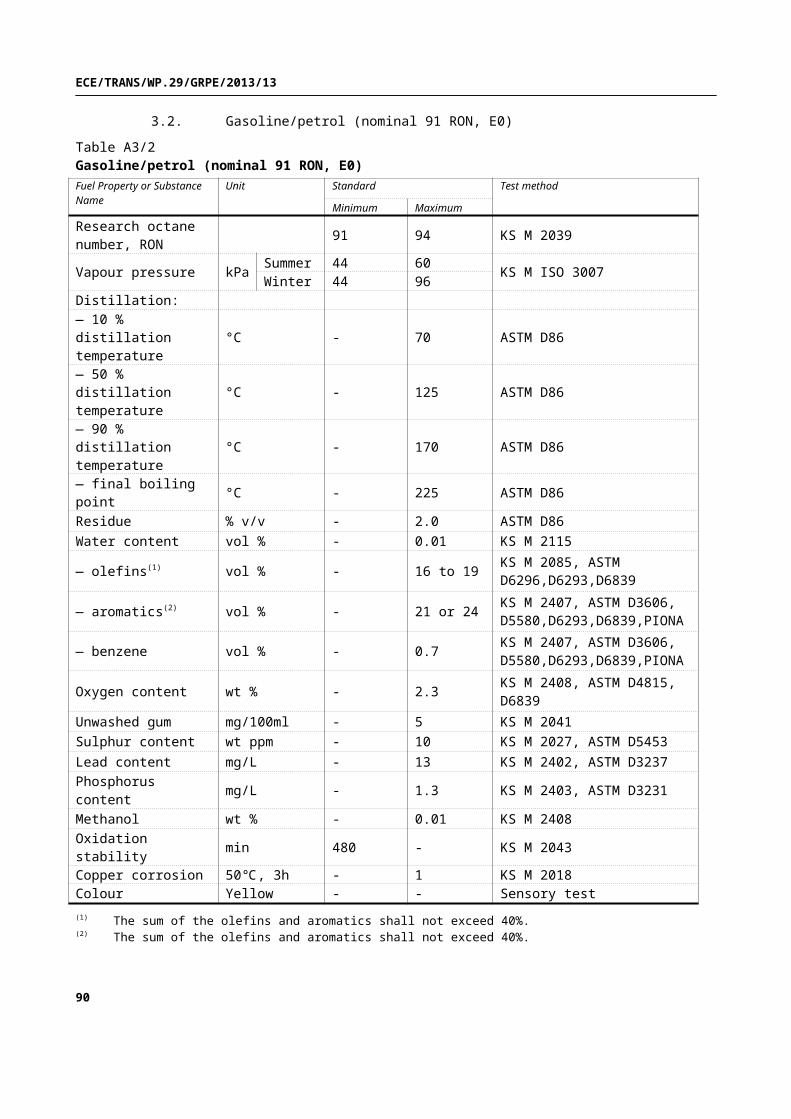
ECE/TRANS/WP.29/GRPE/2013/13
Annex 4
Road load and dynamometer setting
1. Scope
This Annex describes the determination of the road load of a test vehicle and the transfer of that road load to a chassis dynamometer.
2. Terms and definitions
For the purpose of this document, the terms and definitions given in ISO 3833 and in section 3. of this GTR apply.
3. Measurement criteria
3.1. Required overall measurement accuracy
The required overall measurement accuracy shall be as follows:
(a) vehicle speed: ± 0.5 km/h or ± 1 per cent, whichever is greater;
(b) time accuracy: min. ± 10 ms; time resolution: min. ± 0.01 s;
(c) wheel torque (per torque meter): ± 3 Nm or ± 0.5 per cent of the maximum measured torque, whichever is greater;
(d) wind speed: ± 0.3 m/s;
(e) wind direction: ± 3°;
(f) atmospheric temperature: ± 1 K;
(g) atmospheric pressure: ± 0.3 kPa;
(h) vehicle mass: ± 10 kg; (± 20 kg for vehicles > 4,000 kg)
(i) tyre pressure: ± 5 kPa;
(j) product of aerodynamic drag coefficient and frontal projected area (A f × Cd): ± 2 per cent;
(k) chassis dynamometer roller speed: ± 0.5 km/h or ± 1 per cent, whichever is greater;
(l) chassis dynamometer force: ± 10 N or ± 0.1 per cent of full scale, whichever is greater.
[3.2. Wind tunnel criteria
The wind tunnel used for the determination of the product of aerodynamic drag coefficient Cd and frontal area A f within the road load vehicle family shall meet the criteria in this section.
3.2.1. Wind velocity
The wind velocity during a measurement shall remain within ± 2 km/h at the center of the test section. The possible wind velocity shall be at least 140 km/h.
3.2.2. Air temperature
90

ECE/TRANS/WP.29/GRPE/2013/13
The air temperature during a measurement shall remain within ± 2 K at the center of the test section. The air temperature distribution at the nozzle outlet shall remain within ± 3K.
3.2.3. Turbulence
For an equally spaced 3 by 3 grid over the entire nozzle outlet, , the turbulence intensity, Tu, shall not exceed one per cent. See Figure A4/1.
Figure A4/1Turbulence intensity
Tu= u'
U ∞
where:
Tu is turbulence intensity;
u' is turbulent velocity fluctuation, m/s;
U∞ is free flow velocity, m/s.
3.2.4. Solid blockage
The vehicle blockage fraction, ε sb, expressed as the quotient of the vehicle frontal area and the area of the nozzle outlet as shown in the following equation, shall not exceed 35 per cent.
ε sb=A f
Anozzle× 100
where:
ε sb is vehicle blockage in per cent;
A f is frontal area of vehicle in m²;
Anozzle is the area of nozzle outlet in m².
3.2.5. Rotating wheels
To determine the aerodynamic influence of the wheels properly, the wheels of the test vehicle shall rotate at such a speed that the resulting vehicle velocity is within a ± 3 km/h tolerance of the wind velocity.
3.2.6. Moving belt
91
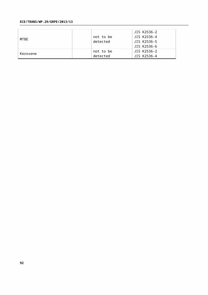
ECE/TRANS/WP.29/GRPE/2013/13
To simulate the fluid flow at the underbody of the test vehicle, the wind tunnel shall have a moving belt extending from the front to the rear of the vehicle. The velocity of the moving belt shall be within ± 3 km/h of the wind velocity.
3.2.7. Fluid flow angle
At 9 equally distributed points over the nozzle area, the root mean square deviation of both angles (Y-, Z-plane) α and β at the nozzle outlet shall not exceed 1°.
3.2.8. Air pressure
At 9 equally distributed points over the nozzle area, the root mean square deviation of the total pressure at the nozzle outlet shall not exceed
two per cent. σ Pt(∆ Pt
q )≤2 per cent
where:
σ Pt is the standard deviation of the total pressure;
∆ Pt is the variation of total pressure between the measurement points;
q is the dynamic pressure.
The pressure coefficient cp over a distance from 2 m ahead and 2 m behind the vehicle shall not deviate more than ± 1 per cent.
ε cp=cpx=2m
cpx=−2 m× 100
where:
cp is the pressure coefficient, N/m².
3.2.9. Boundary layer thickness
At x=0 (balance center point), the wind velocity shall have at least 99 per cent of the inflow velocity 30 mm above the wind tunnel floor.
δ 99 ( x=0 m) ≤ 30 mm
where:
δ 99 is the distance perpendicular to the road, where 99 per cent of free stream velocity is reached (boundary layer thickness).
3.2.10. Restraint system
The restraint system mounting shall not be in front of the vehicle. The relative blockage fraction for the restraint system, ε restr, shall not exceed 10 per cent of the vehicle frontal area.
ε restr=A restr
A f×100
where:
ε restr is the relative blockage of the restraint system;
92

ECE/TRANS/WP.29/GRPE/2013/13
Arestr is the frontal area of the restraint system projected on the nozzle face, m²;
A f is the frontal area of the vehicle in m².
3.2.11. Measurement accuracy in x-direction
At a velocity of 140 km/h, the inaccuracy of the resulting force in the x-direction shall not exceed ± 5 N. The resolution of the measured force shall be within ± 3 N.
3.2.12. Measurement repeatability
The repeatability of the measured force shall be within ± 3 N].
4. Road load measurement on road
4.1. Requirements for road test
4.1.1. Atmospheric conditions for road test
4.1.1.1. Permissible wind conditions
The maximum permissible wind conditions for road load determination are described in 4.1.1.1.1. and 4.1.1.1.2.
In order to determine the applicability of the anemometry type to be used, the average wind speed shall be determined by continuous wind speed measurement, using a recognized meteorological instrument, at a location and height above the road level alongside the test road where the most representative wind conditions will be experienced.
If tests in opposite directions cannot be performed at the same part of the test track (e.g. on an oval test track with an obligatory driving direction), wind speed and direction at each part of the test track shall be measured. In this case the higher measured value determines the type of anemometry to be used and the lower value the criteria for the allowance of waiving of wind correction.
4.1.1.1.1. Permissible wind conditions when using stationary anemometry
Stationary anemometry shall be used only when wind speeds average less than 5 m/s and peak wind speeds are less than 8 m/s. In addition, the vector component of the wind speed across the test road shall be less than 2 m/s. The wind correction shall be conducted as given in 4.5.3. Wind correction may be waived when the lowest average wind speed is 3 m/s or less.
4.1.1.1.2. Permissible wind conditions when using on-board anemometry
A device as described in section 4.3.2. of this Annex shall be used. The overall average wind speed during the test over the test road shall be less than [7] m/s with peak wind speeds of less than [10] m/s. In addition, the vector component of the wind speed across the road shall be less than [4] m/s.
4.1.1.2. Atmospheric temperature
The atmospheric temperature should be within the range of 278 up to and including 313 K.
Contracting Parties may deviate from the upper range by ± 5 K on regional level.
93

ECE/TRANS/WP.29/GRPE/2013/13
At its option, a manufacturer may choose to perform coastdowns between 274 and 278 K.
4.1.2. Test road
The road surface shall be flat, clean, dry and free of obstacles or wind barriers that might impede the measurement of the running resistance, and its texture and composition shall be representative of current urban and highway road surfaces. The test road longitudinal slope shall not exceed 1 per cent. The local slope between any points 3 m apart shall not deviate more than 0.5 per cent from this longitudinal slope. If tests in opposite directions cannot be performed at the same part of the test track (e.g. on an oval test track with an obligatory driving direction), the sum of the longitudinal slopes of the parallel test track segments shall be between 0 and an upward slope of 0.1 per cent. The maximum camber of the test road shall be 1.5 per cent.
4.2. Preparation
4.2.1. Test vehicle
A test vehicle (vehicle H) shall be selected from the CO2 vehicle family (see section 5.6. of the GTR) with the combination of road load relevant characteristics (e.g. mass, aerodynamic drag and tyre rolling resistance) producing the highest cycle energy demand .
At the request of the manufacturer, the CO2 interpolation method may be applied for individual vehicles in the CO2 vehicle family (see paragraph 1.2.3.1. of Annex 6 and section 3.2.3.2. of Annex 7). In that case, the road load shall also be determined on a test vehicle (vehicle L) having a combination of road load relevant characteristics producing the lowest cycle energy demand .
Each test vehicle shall conform in all its components with the production series, or, if the vehicle is different from that, a full description shall be recorded. If the manufacturer requests to use the CO2 interpolation method, the increase or decrease in the product of the aerodynamic drag coefficient (Cd) and frontal area ( A f ), m2, expressed as ∆ f 2 for all of the optional equipment in the CO2 vehicle family having an influence on the aerodynamic drag of the vehicle shall be recorded.
4.2.1.1. Movable aerodynamic body parts
Movable aerodynamic body parts on test vehicles shall operate during road load determination as intended under WLTP Type 1 test conditions (test temperature, speed and acceleration range, engine load, etc.).
Appropriate requirements shall be added here if future vehicles are equipped with movable aerodynamic options whose influence on aerodynamic drag justify the need for further requirements.
4.2.1.2 Wheels
If the manufacturer is not able to measure the aerodynamic drag of individual rotating wheels, the wheel with the highest expected aerodynamic drag shall be selected for test vehicles H and L.
As a guideline, the highest aerodynamic drag may be expected for a wheel rim with a) the largest width, b) the largest diameter, and c) the most open structure design (in that order of importance).
94

ECE/TRANS/WP.29/GRPE/2013/13
4.2.1.3. Weighing
Before and after the road load determination procedure, the selected vehicle shall be weighed, including the test driver and equipment, to determine the average mass mav. The mass of the vehicle shall be equal to or higher than the target test mass (TM H or TM L, calculated according to paragraph 4.2.1.3.1. below) at the start of the road load determination procedure.
For the test mass correction factor determination in section 4.5.4. of this Annex, the actual test masses TM H , actual and TM L ,actual will be used, i.e. the average mass mav for the respective test masses.
4.2.1.3.1. Vehicle test mass
The maximum and minimum values of test mass TM for vehicle H and vehicle L of the CO2 vehicle family shall be calculated as follows:
TM H shall be the sum of the mass in running order, the mass of the optional equipment, 25 kg, and the mass representative of the payload.
TM L shall be the sum of the mass in running order, 25 kg, and the mass representative of the payload.
The mass representative of the payload shall be 15per cent (for category 1 vehicles) and 28 per cent (for category 2 vehicles) of the difference between the technically permissible maximum laden mass (LM) and the sum of the mass in running order, 25 kg, and the mass of the optional equipment for vehicle H .
4.2.1.4. Test vehicle configuration
The test vehicle configuration shall be recorded and shall be used for any subsequent testing.
4.2.1.5. Test vehicle condition
4.2.1.5.1. Run-in
The test vehicle shall be suitably run-in for the purpose of the subsequent test for at least 10,000 but no more than 80,000 km.
4.2.1.5.1.1. At the request of the manufacturer, a vehicle with a minimum of 3,000 km may be used.
4.2.1.5.2. Manufacturer's specifications
The vehicle shall conform to the manufacturer’s intended production vehicle specifications regarding tyre pressures (paragraph 4.2.2.3. below), wheel alignment, ground clearance, vehicle height, drivetrain and wheel bearing lubricants, and brake adjustment to avoid unrepresentative parasitic drag.
4.2.1.5.3. Alignment
If an alignment parameter is adjustable (track, camber, caster), it shall be set to the nominal value of the manufacturer’s intended production vehicle. In absence of a nominal value, it shall be set to the mean of the values recommended by the manufacturer.
Such adjustable parameter(s) and set value shall be recorded.
95

ECE/TRANS/WP.29/GRPE/2013/13
4.2.1.5.4. Closed panels
During the road test, the engine bonnet, manually-operated moveable panels and all windows shall be closed.
4.2.1.5.5. Coastdown mode
If the determination of dynamometer settings cannot meet the criteria described in sections 8.1.3. or 8.2.3. of this Annex due to non-reproducible forces, the vehicle shall be equipped with a vehicle coastdown mode. The coastdown mode shall be approved and recorded by the responsible authority.
4.2.1.5.5.1. If a vehicle is equipped with a vehicle coastdown mode, it shall be engaged both during road load determination and on the chassis dynamometer.
4.2.2. Tyres
4.2.2.1. Tyre selection
The selection of tyres shall be based on their rolling resistances measured according to Regulation No. 117-02, or a similar internationally-accepted equivalent and the rolling resistance coefficients shall be aligned according to the respective regional procedures (e.g. EU 1235/2011), and categorised according to the rolling resistance classes in Table 2. If tyres from multiple categories are offered for the CO2 vehicle family, a tyre shall be selected from the class having the highest RRC class value. See Table A4/1.
Table A4/1Classes of rolling resistance coefficients (RRC) for tyre categories C1, C2 and C3, kg/tonne
Class C1 range C2 range C3 range
1 RRC ≤ 6.5 RRC ≤ 5.5 RRC ≤ 4.0
2 6.5 < RRC ≤ 7.7 5.5 < RRC ≤ 6.7 4.0 < RRC ≤ 5.0
3 7.7 < RRC ≤ 9.0 6.7 < RRC ≤ 8.0 5.0 < RRC ≤ 6.0
4 9.0 < RRC ≤ 10.5 8.0 < RRC ≤ 9.2 6.0 < RRC ≤ 7.0
5 10.5 < RRC ≤ 12.0 9.2 < RRC ≤ 10.5 7.0 < RRC ≤ 8.0
6 RRC > 12.0 RRC > 10.5 RRC > 8.0
Class C1 class value C2 class value C3 class value
1 RRC = 5.9 RRC = 4.9 RRC = 3.5
2 RRC = 7.1 RRC = 6.1 RRC = 4.5
3 RRC = 8.4 RRC = 7.4 RRC = 5.5
4 RRC = 9.8 RRC = 8.6 RRC = 6.5
5 RRC = 11.3 RRC = 9.9 RRC = 7.5
6 RRC = 12.9 RRC = 11.2 RRC = 8.5
The actual rolling resistances values for the tyres fitted to the test vehicles shall be used as input for the calculation procedure of the CO2 interpolation method in section 3.2.3.2 of Annex 7. For individual vehicles in the CO2
vehicle family, the CO2 interpolation method shall be based on the RRC class value for the tyres fitted to the individual vehicle.
96

ECE/TRANS/WP.29/GRPE/2013/13
4.2.2.2. Tyre condition
Tyres used for the test shall:
(a) not be older than 2 years after production date;
(b) not be specially conditioned or treated (e.g. heated or artificially aged), with the exception of grinding in the original shape of the tread;
(c) be run-in on a road for at least 200 km before road load determination;
(d) have a constant tread depth before the test between 100 and 80 per cent of the original tread depth over the full tread width of the tyre.
4.2.2.2.1. After measurement of tread depth, driving distance shall be limited to 500 km. If 500 km are exceeded, tread depth shall be measured again.
4.2.2.2.2. Tread depth shall be measured before performing another road load determination with the same tyres but on another vehicle.
4.2.2.3. Tyre pressure
The front and rear tyres shall be inflated to the lower limit of the tyre pressure range for the selected tyre at the coastdown test mass, as specified by the vehicle manufacturer.
4.2.2.3.1. Tyre-pressure adjustment
If the difference between ambient and soak temperature is more than 5 K, the tyre pressure shall be adjusted as follows:
(a) the tyres shall be soaked for more than 1 h at 10 per cent above the target pressure;
(b) prior to testing, the tyre pressure shall be reduced to the inflation pressure as specified in 4.2.2.3., adjusted for difference between the soaking environment temperature and the ambient test temperature at a rate of 0.8 kPa per 1 K using the following equation:
∆ pt=0.8 × ( T soak−T amb )where:
∆ pt is the tyre pressure adjustment added to the tyre pressure defined in paragraph 4.2.2.3. of this Annex, kPa;
0.8 is the pressure adjustment factor, kPa/K;
T soak is the tyre soaking temperature, degrees Kelvin (K);
T amb is the test ambient temperature, degrees Kelvin (K);
(c) between the pressure adjustment and the vehicle warm-up, the tyres shall be shielded from external heat sources including sun radiation.
4.2.3. Instrumentation
Any instruments, especially those installed outside the vehicle, shall be installed on the vehicle in such a manner as to minimise effects on the aerodynamic characteristics of the vehicle.
4.2.4. Vehicle warm-up
97

ECE/TRANS/WP.29/GRPE/2013/13
4.2.4.1. On the road
Warming up shall be performed by driving the vehicle only.
4.2.4.1.1. Before warm-up, the vehicle shall be decelerated with the clutch disengaged or an automatic transmission in neutral by moderate braking from 80 to 20 km/h within five to ten seconds. After this braking, there shall be no further manual adjustment of the braking system.
4.2.4.1.2. Warming up and stabilization
All vehicles shall be driven at 90 per cent of the maximum speed of the applicable WLTC. The vehicle may be driven at 90 per cent of the maximum speed of the next higher phase (see Table A4/2) if this phase is added to the applicable WLTC warm-up procedure as defined in section 7.3.4. of this Annex. The vehicle shall be warmed up for at least 20 min until stable conditions are reached.
Table A4/2Warming up and stabilization across phases
Vehicle class Applicable WLTC90 per cent of maximum
speed Next higher phase
Class1 Low1 & Medium1 58 km/h NA
Class2 Low2 & Medium2 & High2
& Extra High2 111 km/h NA
Low2 & Medium2 & High2 77 km/h Extra high(111 km/h)
Class3 Low3 & Medium3 & High3
& Extra High3 118 km/h NA
Low3 & Medium3 & High3 88 km/h Extra high(118 km/h)
4.2.4.1.3. Criteria for stable condition
Refer to paragraph 4.3.1.4.2. of this Annex.
4.3. Measurement and calculation of total resistance by the coastdown method
The total resistance shall be determined by using the multi-segment (section 4.3.1. of this Annex) or on-board anemometer (section 4.3.2. of this Annex) method.
4.3.1. Multi-segment method with stationary anemometry
4.3.1.1. Selection of reference speeds for road load curve determination
In order to obtain a road load curve as a function of vehicle speed, a minimum of six reference speeds v j ( j=1, j=2, etc.) shall be selected. The highest reference speed shall not be lower than the highest speed of the speed range, and the lowest speed point shall not be higher than the lowest speed of the speed range. The interval between each speed point shall not be greater than 20 km/h.
4.3.1.2. Data collection
During the test, elapsed time and vehicle speed shall be measured and recorded at a minimum rate of 5 Hz.
4.3.1.3. Vehicle coastdown procedure
98

ECE/TRANS/WP.29/GRPE/2013/13
4.3.1.3.1. Following the vehicle warm-up procedure (section 4.2.4. of this Annex), and immediately prior to each test measurement, the vehicle may be driven at the highest reference speed up to a maximum of one minute. The vehicle shall be accelerated to at least 5 km/h above the speed at which the coastdown time measurement begins (vi+v) and the coastdown shall be started immediately.
4.3.1.3.2. During coastdown, the transmission shall be in neutral, and the engine shall run at idle. Steering wheel movement shall be avoided as much as possible, and the vehicle brakes shall not be operated until the speed drops below (v j - ∆v).
4.3.1.3.3. The test shall be repeated until the coastdown data satisfy the statistical accuracy requirements as specified in paragraph 4.3.1.4.2..
4.3.1.3.4. Although it is recommended that each coastdown run be performed without interruption, split runs are permitted if data cannot be collected in a continuous way for the entire speed range. For split runs, care shall be taken so that vehicle conditions remain as stable as possible at each split point.
4.3.1.4. Determination of total resistance by coastdown time measurement
4.3.1.4.1. The coastdown time corresponding to the velocity v j as the elapsed time from the vehicle velocity (vi+v) to (vi−v) shall be measured. It is recommended that v=5 km/h with the option of v=10 km/h when the vehicle velocity is more than 60 km/h. .
4.3.1.4.2. These measurements shall be carried out in both directions until a minimum of three consecutive pairs of figures have been obtained which satisfy the statistical accuracy p, in per cent, defined below.
p=h × σ√n
× 100∆ t j
≤ 3 per cent
where:
p is the statistical accuracy;
n is the number of pairs of measurements;
∆ t j is the mean coastdown time at velocity vi, seconds, given by the
equation ∆ t j=1n∑i=1
n
∆ t ji, where ∆ t ji is the harmonised average
coastdown time of the ith pair of measurements at velocity vi,
seconds (s), given by the equation: ∆ t ji=
2
( 1∆t jai )+( 1
∆ t jbi ) . ∆ t jai
and ∆ t jbi are the coastdown times of the ith measurement at speed vi, seconds (s), in each direction, respectively;
σ is the standard deviation, expressed in seconds (s), defined by:
σ=√ 1n−1∑i=1
n
(∆ t ji−∆ t j) ²
h is a coefficient given in Table A4/3.
99

ECE/TRANS/WP.29/GRPE/2013/13
Table A4/3Coefficient h as function of nn h h/√n n h h/√n3 4.3 2.48 10 2.2 0.73
4 3.2 1.60 11 2.2 0.66
5 2.8 1.25 12 2.2 0.64
6 2.6 1.06 13 2.2 0.61
7 2.5 0.94 14 2.2 0.59
8 2.4 0.85 15 2.2 0.57
9 2.3 0.77
4.3.1.4.3. If during a measurement in one direction any external factor or driver action occurs which influences the road load test, that measurement and the corresponding measurement in the opposite direction shall be rejected.
4.3.1.4.4. The total resistances, F ja and F jb at velocity vi in directions a and b, in Newton (N), are determined by the equations:
F ja=−13.6
× (mav+mr ) × 2× ∆ v∆ t ja
and
F jb=−13.6
× (mav+mr )× 2× ∆ v∆t jb
where:
F ja is the total resistance at velocity (j) in direction a, in Newton (N);
F jb is the total resistance at velocity (j) in direction b, in Newton (N);
mav is the average of the test vehicle masses at the beginning and end of road load determination, kg;
mr is the equivalent effective mass of all the wheels and vehicle components rotating with the wheels during coastdowns on the road, in kilograms (kg); mr shall be measured or calculated using an appropriate technique agreed by the responsible authority. Alternatively, mr may be estimated to be three per cent of the unladen vehicle mass in running order + 25 kg for the CO2 vehicle family;
∆ t ja and ∆ t jb are the mean coastdown times in directions a and b, respectively,corresponding to velocity vi, seconds (s), given by
the equations ∆ t ja=1n∑i=1
n
∆ t jai and ∆ t jb=1n∑i=1
n
∆ t jbi.
100

ECE/TRANS/WP.29/GRPE/2013/13
4.3.1.4.5. The following equation shall be used to compute the average total resistance, where the harmonised average of the alternate coastdown time shall be used .
F j=−13.6
× (mav+mr ) × 2× ∆ v∆ t j
where:
∆ t j is the harmonised average of alternate coastdown time measurements
at velocity vi, seconds (s), given by ∆ t j=
21
∆ t ja+ 1
∆t jb
where ∆ t ja
and ∆ t jb are the coastdown times at velocity vi, seconds (s), in each direction, respectively;
mav is the average of the test vehicle masses at the beginning and end of road load determination, kg;
mr is the equivalent effective mass of all the wheels and vehicle components rotating with the wheels during coastdowns on the road, in kilograms (kg); mr shall be measured or calculated using an appropriate technique. Alternatively, mr may be estimated to be three
per cent of the unladen vehicle mass (UM ) for the vehicle family.
The coefficients f 0, f 1 and f 2 in the total resistance equation shall be calculated with a least-squares regression analysis.
4.3.2. On-board anemometer-based coastdown method
The vehicle shall be warmed up and stabilised according to section 4.2.4. of this Annex. Calibration of instrumentation will take place during this time.
4.3.2.1. Additional instrumentation for on-board anemometry
The anemometer shall be calibrated by means of operation on the test vehicle where such calibration occurs during the warm-up for the test.
4.3.2.1.1. Relative wind speed shall be measured to an accuracy of 0.3 m/s and shall be recorded at a minimum rate of 1 Hz. Calibration of the anemometer shall include corrections for vehicle blockage.
4.3.2.1.2. Wind direction shall be relative to the direction of the vehicle. Relative wind direction (yaw) shall be measured to an accuracy of 3 degrees and recorded to a resolution of 1 degree; the "dead band" of the instrument shall not exceed 10 degrees and shall be directed toward the rear of the vehicle.
4.3.2.1.3. Before the coastdown, the anemometer shall be calibrated for speed and yaw offset as specified in IS0 10521 Annex A.
4.3.2.1.4. Anemometer blockage shall be corrected for in the calibration procedure as described in ISO 10521-1:2006(E) Annex A.
4.3.2.2. Selection of speed range for road load curve determination
The test speed range as specified in paragraph 4.3.1.1. above shall be selected.
101

ECE/TRANS/WP.29/GRPE/2013/13
4.3.2.3. Data collection
Various data shall be measured and recorded during the procedure. Elapsed time, vehicle speed, and air velocity (speed, direction) relative to the vehicle, shall be measured at 5 Hz. Ambient temperature shall be synchronised and sampled at a minimum of 1 Hz.
4.3.2.4. Vehicle coastdown procedure
Vehicle coastdown shall be conducted as specified in paragraphs 4.3.1.3.1. to 4.3.1.3.4. above with an on-board anemometer installed on the vehicle. A minimum of ten runs shall be made in alternating directions; five runs in each direction. Wind-corrected coastdown data must satisfy the statistical accuracy requirements as specified in paragraph 4.3.1.4.2. above. The anemometer shall be installed in a position such that the effect on the operating characteristics of the vehicle is minimised.
The anemometer shall be installed according to (a) or (b) below:
(a) using a boom approximately 2 m in front of the vehicle’s forward aerodynamic stagnation point.
(b) on the roof of the vehicle at its centreline. If possible, the anemometer shall be mounted within 15 cm. from the top of the windshield.
In the event that position (b) is used, the coastdown results shall be analytically adjusted for the additional aerodynamic drag induced by the anemometer. The adjustment shall be made by testing the coastdown vehicle in a wind tunnel both with and without the anemometer installed (same position as used on the track), where the calculated difference will be the incremental drag coefficient (Cd), which combined with the frontal area can be used to correct the coastdown results.
4.3.2.5. Determination of the equation of motion
Symbols used in the on-board anemometer equations of motion are listed in Table A4/4.
102

ECE/TRANS/WP.29/GRPE/2013/13
Table A4/4Symbols used in the on-board anemometer equations of motion
Symbol
Unit Description
A f frontal areaa0…
coefficients for aerodynamic drag, as a function of yaw angle
Am coefficient of mechanical dragBm
(kmcoefficient of mechanical drag
Cm(km
coefficient of mechanical drag
Baro barometric pressureCd (Y ) coefficient of aerodynamic drag at yaw angle YD dragDaero aerodynamic dragDf front axle drag (including driveline)D grav gravitational dragDmech mechanical dragDr rear axle drag (including driveline)Dtire tyre rolling resistance(dv /dt ) acceleration
g gravitational constant
m mass of vehicleme effective vehicle mass (including rotating components)ρ air density
t timeT temperaturev vehicle speedvr apparent wind speed relative to vehicleY yaw angle of apparent wind relative to direction of vehicle
4.3.2.5.1. General form
The general form of the equation of motion can be written as shown in the equation below:
me ( dvdt )=Dmech+ Daero
where:
Dmech=Dtyre+Df +D r;
Daero=(12 ) ρ Cd (Y ) A vr
2;
me=¿effective vehicle mass.
4.3.2.5.2. Mechanical drag modelling
Although mechanical drag consists of separate components representing tire (Dtire), front and rear axle frictional losses (Df and Dr, including transmissions losses), it can be modelled as a three-term polynomial with respect to speed (v), as in the equation below:
103

ECE/TRANS/WP.29/GRPE/2013/13
Dmech=Am+Bm v+Cm v2
where:
Am, Bm, and Cm are determined in the data analysis using the least-squares method. These constants reflect the combined driveline and tyre drag.
4.3.2.5.3. Aerodynamic drag modelling
The aerodynamic drag coefficient, Cd(Y), is modelled as a four-term polynomial with respect to yaw angle (Y , deg), as in the equation below:
Cd (Y )=a0+a1 Y +a2 Y 2+a3 Y 3+a4 Y 4
where a0 to a4 are constant coefficients whose values are determined in the data analysis. The aerodynamic drag coefficient is combined with the vehicle frontal area ( A f ), and the relative wind velocity (vr) to determine the aerodynamic drag (Daero) according to the following two equations:
Daero=( 12 ) ρ A f vr
2Cd(Y )
Daero=( 12 ) ρ A f vr
2(a0+a1Y +a2Y 2+a3Y 3+a4 Y 4)
4.3.2.5.4. Substituting, the final form of the equation of motion becomes:
me ( dvdt )=¿
¿ Am+Bm v+Cm v2+( 12 ) ρ Avr
2(a0+a1 Y +a2 Y 2+a3 Y 3+a4 Y 4)
4.3.2.6. Data reduction
Techniques for analysing coastdown data shall be employed in the determination of the coefficients used to describe the road load force. A three term equation shall be generated to describe the road load force as a function of velocity, F=A+Bv+C v2, corrected to standard ambient temperature and pressure conditions, and still air.
4.3.2.6.1. Determining calibration coefficients
If not previously determined, calibration factors to correct for vehicle blockage shall be determined for relative wind speed and yaw angle. Vehicle speed (v), relative wind velocity (vr¿and yaw (Y ) measurements during the warm-up phase of the test procedure shall be recorded. Paired runs in alternate directions on the test track at a constant velocity of 80 km/h shall be performed, and averages for v, vr and Y for each run shall be determined. Calibration factors that minimize the total errors in head and cross winds over all the run pairs, i.e. the sum of (hea di – head i+1 )2, etc., shall be selected where headi and headi+1 refer to wind speed and wind direction from the paired test runs in opposing directions during the vehicle warm-up/stabilisation prior to testing..
104

ECE/TRANS/WP.29/GRPE/2013/13
4.3.2.6.2. Deriving second by second observations
From the periodic data collected during the coastdown runs, values for v,
( dvdt ), vr
2, and Y shall be determined by applying calibration factors and data
filtering to adjust samples to 1 Hz.
4.3.2.6.3. Preliminary analysis
Using a linear least-squares regression technique, all data points shall be analysed at once. Am , Bm , Cm , a0 , a1, a2 , a3 ,and a4 given
M e ,( dvdt ), v , vr ,andρ shall be determined.
4.3.2.6.4. Identifying "outliers"
For each data point, a predicted force, me ( dvdt ), shall be calculated and
compared to that observed. Data points with excessive deviations, e.g., over three standard deviations, shall be flagged.
4.3.2.6.5. Data filtering
If desired, appropriate data filtering techniques may be employed. Remaining data points shall be smoothed out.
4.3.2.6.6. Elimination of extreme data points
Data points with yaw angles greater than ± 20 degrees from the direction of vehicle travel shall be flagged. Data points with relative winds less than + 5 km/h (to avoid backwind conditions) shall also be flagged. Data analysis shall be restricted to vehicle speeds from 115 to 15 km/h.
4.3.2.6.7. Final data analysis
All data which has not been flagged shall be analysed using a linear least-
squares regression technique. Given M e ,( dvdt ), v , vr ,andρ, Am , Bm , Cm ,
a0 , a1 , a2 , a3 ,and a4 shall be determined.
4.3.2.6.8. Constrained analysis option
In a constrained analysis, the vehicle frontal area ( A) and the drag coefficient (Cd) are fixed at values which have been previously determined.
4.3.2.6.9. Correction to reference conditions
Equations of motion shall be corrected for reference conditions as specified in section 4.5. of this Annex.
4.4. Measurement of running resistance using the torque meter method
As an alternative to the coastdown methods, the torque meter method may also be used in which the running resistance is determined by measuring wheel torque on the driven wheels at various constant speeds with time periods of at least five seconds.
4.4.1. Installation of torque meter
105

ECE/TRANS/WP.29/GRPE/2013/13
Wheel torque meters shall be installed between the wheel hub and the rim of each driven wheel, measuring the required torque to keep the vehicle at a constant speed.
4.4.2. Procedure and data sampling
4.4.2.1. Speed selection
The range of selected reference speeds v j ( j=1, j=2, etc.) where the running resistance is to be measured shall start at 15 km/h and cover the entire speed range of the applicable test cycle, while the difference between v j and v j+1 is 20 km/h or less.
4.4.2.2. Start of data collection
Data collection shall be started after a vehicle warm-up according to section . 4.2.4. of this Annex.
The reference speeds will be measured in a descending order. Upon the request of the manufacturer, stabilization periods are allowed between measurements but the stabilization speed shall not exceed the speed of the next reference speed.
4.4.2.3. Data collection
Data sets consisting of actual speed v ji, actual torque C ji and time over a period of at least 5 s shall be recorded for every v j at a sampling frequency of at least 10 Hz. The data sets collected over one time period for a reference speed v j will be referred to as one measurement.
4.4.2.4. Velocity deviation
The velocity deviation v ji from the mean velocity v jm (section 4.4.3. of this Annex) shall be within the values in Table A4/5.
Table A4/5Velocity deviation
Time period, seconds Velocity deviation, km/h
5 - 10 ± 0.2
10 - 15 ± 0.4
15 - 20 ± 0.6
20 - 25 ± 0.8
25 - 30 ± 1.0
≥ 30 ± 1.2
4.4.3. Calculation of mean velocity and mean torque
4.4.3.1. Calculation process
Mean velocity v jm, (km/h) and mean torque C jm, (Nm) over a time period, shall be calculated from the data sets collected in paragraph 4.4.2.3. above as follows:
106
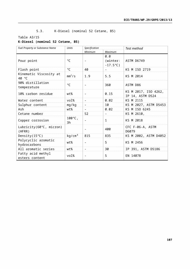
ECE/TRANS/WP.29/GRPE/2013/13
v jm=1k ∑i=1
k
v ji
and
C jm=1k ∑i=1
k
C ji−C js
where:
v ji is vehicle speed of the ith data set, km/h;
k is the number of data sets;
C ji is torque of the ith data set, Nm;
C js is the compensation term for speed drift, Nm, given by the following equation C js=(mav+mr ) ×α j r j.
C js shall be no greater than five per cent of the mean torque before compensation, and may be neglected if α j is not greater than ± 0.005 m/s2.
mav and mr are the average test vehicle mass and the equivalent effective mass, in kg, , respectively, defined in paragraph 4.3.1.4.4. above.
r 'is the dynamic radius of the tyre, in meters (m), given by the
equation r '= 13.6
×v jm
2 × πN, where N is the rotational frequency of
the driven tyre, in s-1;
α j is the mean acceleration, in metres per second squared (m/s2), which shall be calculated by the equation
∝ j=1
3.6×
k∑i=1
k
ti v ji−∑i=1
k
t i∑i=1
k
v ji
k×∑i=1
k
t i2−[∑i=1
k
t i]2 , where t iis the time at which
the ith data set was sampled, seconds (s).
4.4.3.2. Accuracy of measurement
These measurements shall be carried out in opposite directions until a minimum of four consecutive figures at each vi and in both directions (a and b) have been obtained, for which C j satisfies the accuracy ρ, in per cent, according to the equation:
ρ=t × s√n
× 100C j
≤ 3 per cent
where:
n is the number pairs of measurements for C jm;
107

ECE/TRANS/WP.29/GRPE/2013/13
C j is the running resistance at the speed v j, expressed in Nm, given by
the equation C j=1n∑i=1
n
C jmi, where C jmi is the average torque of the
ith pair of measurements at speed v j, expressed in Nm and given by
C jmi=12
× (C jmai+C jmbi )¿where C jmai and C jmbi are the mean
torques of the ith measurement at speed v j determined in paragraph 4.4.3.1. above for each direction, a and b respectively, expressed in Nm);
s is the standard deviation, expressed in Nm, defined by the equation
s=√ 1k−1∑i=1
k
(C jmi−C j )2;
t is a coefficient from Table A4/3 in paragraph 4.3.1.4.2. above.
4.4.3.3. Validity of the measured average speed
The average speed v jmi, shall not deviate from its mean, v j by more than ± 1 km/h or two per cent of the average speed v jmi, whichever is greater. The values of v jmi and v j shall be calculated as follows:
v j=1n∑i=1
n
v jmi
v jmi=12
× ( v jmai+v jmbi )
where v jmai and v jmai are the mean speeds of the ith pair of measurements at velocity v j determined in paragraph 4.4.3.1. above for each direction, a and b respectively, expressed in km/h.
4.4.4. Running resistance curve determination
The following least-squares regression curves for each direction a and b shall be fitted using the least squares method to all the data pairs (v jm, C jma) and (v jm,, C jmb) at all at all reference speeds v j, ( j=1, j=2, etc.) described in paragraph 4.3.1.1. above to determine the coefficients c0 a, c0 b, c1a, c1b, c2 a and c2 b:
Ca=c0 a+c1 a v+c2 b v2
Cb=c0 b+c1 b v+c2 b v2
where:
Ca and Cb are the running resistances in directions a and b, Nm;
c0 a and c0 b are constant terms in directions a and b, Nm;
c1 a and c1 b are the coefficients of the first-order term in directions a and b, Nm (h/km);
108

ECE/TRANS/WP.29/GRPE/2013/13
c2 a and c2 b are the coefficients of the second-order term in directions a and b, Nm (h/km)2;
v is vehicle velocity, km/h.
The average total torque equation is calculated by the following equation:
Cavg=c0+c1 v+c2 v2
where the average coefficients c0, c1 and c2 shall be calculated using the following equations:
c0=c0 a+c0 b
2
c1=c1 a+c1 b
2
c2=c2 a+c2 b
2
The coefficient c1 may be assumed to be zero if the value of c1× v is no greater than three per cent of C at the reference speed(s); in this case, the coefficients c0 and c2 shall be recalculated according to the least squares method.
The coefficients c0, c1 and c2 as well as the coastdown times measured at the chassis dynamometer (see paragraph 8.2.3.3. of this Annex) shall be recorded.
4.5. Correction to reference conditions
4.5.1. Air resistance correction factor
The correction factor for air resistance K2 shall be determined as follows:
K 2=T
293× 100
Pwhere:
T is the mean atmospheric temperature, degrees Kelvin (K);
P is the mean atmospheric pressure, in kPa.
4.5.2. Rolling resistance correction factor
The correction factor, K 0, for rolling resistance, in Kelvin-1 (K-1), may be determined based on empirical data and approved by the responsible authority for the particular vehicle and tyre test, or may be assumed as follows:
K 0=8.6 ×10⁻³
4.5.3. Wind correction with stationary anemometry
4.5.3.1. Wind correction, for absolute wind speed alongside the test road, shall be made by subtracting the difference that cannot be cancelled by alternate runs from the constant term f 0 given in paragraph 4.3.1.4.5. above, or from c0
109

ECE/TRANS/WP.29/GRPE/2013/13
given in paragraph 4.4.4. above. The wind correction shall not apply to the on-board anemometer-based coastdown method.
4.5.3.2. The wind correction resistance w1 for the coastdown method or w2 for the torque meter method shall be calculated by the equations:
w1=3.62 × f 2× vw2 or w2=3.62 ×c2 ×v w
2
where:
w1 is the wind correction resistance for the coastdown method, N;
f 2 is the coefficient of the aerodynamic term determined in section 4.3.1.4.5. of this Annex;
vw is the lower average wind speed of both directions alongside the test road during the test, m/s;
w2 is the wind correction resistance for the torque meter method, Nm;
c2 is the coefficient of the aerodynamic term determined in paragraph 4.4.4. of this Annex.
4.5.4. Test mass correction factor
4.5.4.1. Test vehicle H
The correction factor K 1 for the test mass of test vehicle H shall be determined as follows:
K 1=f 0 ×(1−TM H
TM H ,actual)
where:
f 0 is a constant term, N;
TM H is test mass of the test vehicle H, kg;
TM H , actual is the actual test mass of test vehicle H (the average mass mav; (see paragraph 4.3.1.4.4. of this Annex), kg.
4.5.4.2. Test vehicle L
The correction factor K 1 for the test mass of test vehicle L shall be determined as follows:
K 1=f 0 ×(1−TM L
TM L, actual)
where:
f 0 is a constant term, N;
TM L is test mass of test vehicle L, kg;
TM L ,actual is the actual test mass of the test vehicle L (the average mass mav, see paragraph 4.3.1.4.4. of this Annex), kg.
110

ECE/TRANS/WP.29/GRPE/2013/13
4.5.5. Road load curve correction
4.5.5.1. The curve determined in section 4.3.1.4.5. of this Annex shall be corrected to reference conditions as follows and shall be used as the target coefficients in paragraph 8.1.1.:
F ¿=( (f 0−w1−K1 )+ f 1 v )× (1+K0 (T−293 ) )+K 2 f 2 v2
where:
F ¿ is the corrected total resistance, N;
f 0 is the constant term, N;
f 1 is the coefficient of the first-order term, N (h/km);
f 2 is the coefficient of the second-order term, N (h/km)2;
K 0 is the correction factor for rolling resistance as defined in paragraph 4.5.2. of this Annex;
K 1 is the test mass correction as defined in section 4.5.4. of this Annex;
K 2 is the correction factor for air resistance as defined in paragraph 4.5.1. of this Annex;
v is vehicle velocity, km/h;
w1 is the wind resistance correction as defined in section 4.5.3. of this Annex.
4.5.5.2. The curve determined in paragraph 4.4.4. above shall be corrected to reference conditions as follows:
C ¿=( (c0−w2−K1 )+c1 v )× (1+K0 (T−293 ) )+K2 c2 v ²
where:
C ¿ is the corrected total running resistance, Nm;
c0 is the constant term, Nm;
c1 is the coefficient of the first-order term, Nm (h/km);
c2 is the coefficient of the second-order term, Nm (h/km)2;
K 0 is the correction factor for rolling resistance as defined in paragraph 4.5.2. of this Annex;
K 1 is the test mass correction as defined in section 4.5.4.;
K 2 is the correction factor for air resistance as defined in paragraph 4.5.1. of this Annex;
v is vehicle velocity, km/h;
w2 is the wind correction resistance as defined in section 4.5.3. of this Annex.
5. Method for the calculation of default road load based on vehicle parameters
111

ECE/TRANS/WP.29/GRPE/2013/13
5.1. As an alternative for determining the road load with the coastdown or torque meter method, a calculation method for default road load may be used.
For the calculation of a default road load several parameters such as test mass, width and height from the vehicle shall be used. The default road load (F c) for several speeds v, in km/h , shall be calculated. Reference speeds shall be selected according to § 4.3.1.1 and the default road load (Fc), in N, for these reference speeds vj, in km/h, shall be calculated. The results of the calculated default road load values shall be used for the setting of the chassis dynamometer. A coastdown test on a chassis dynamometer shall be conducted to ensure the correct settings of the chassis dynamometer.
5.2. The default road load force shall be calculated using the following equation:
F c=(0.140 × ( 1+0.00002× v2 ) ×TM )+¿
+( 0.0170× width× height × v2 )where:
F c is the calculated default road load force for a given vehicle velocity v, and it is expressed in Newton (N);
v is vehicle velocity, km/h;
TM test mass, kg;
width vehicle width, m,as defined in 6.2 of Standard ISO 612:1978;
height vehicle height, m, as defined in 6.3 of Standard ISO 612:1978.
6. [RESERVED: Road load measurement using a combination of a wind tunnel and chassis dynamometer]
7. Transferring road load to a chassis dynamometer
7.1. Preparation for chassis dynamometer test
7.1.1. Laboratory condition
7.1.1.1. Roller
The chassis dynamometer roller(s) shall be clean, dry and free from foreign material which might cause tyre slippage. For chassis dynamometers with multiple rollers, the dynamometer shall be run in the same coupled or uncoupled state as the subsequent Type 1 test. Chassis dynamometer speed shall be measured from the roller coupled to the power-absorption unit.
7.1.1.1.1. Tyre slip
Additional weight may be placed on or in the vehicle to eliminate tyre slip. The manufacturer shall perform the load setting on the chassis dynamometer with the additional weight. The additional weight shall be present for both load setting and the emissions tests. The use of any additional weight shall be recorded.
7.1.1.2. Room temperature
112
ECE/TRANS/WP.29/GRPE/2013/13
The laboratory atmospheric temperature shall be at a set point of 296 K and shall not deviate by more than ± 5 K during the test as the standard condition, unless otherwise required by the subsequent test(s).
7.2. Preparation of chassis dynamometer
7.2.1. Inertia mass setting
The equivalent inertia mass of the chassis dynamometer shall be set to the test mass used at the corresponding road load determination if a dual-axis chassis dynamometer is used. In case a single-axis chassis dynamometer is used, the equivalent inertia mass shall be increased by the inertia of the wheels and connected vehicle parts which are not rotating. If m r is estimated at 3 per cent of the mass in running order + 25 kg, UM , the mass added to the inertia setting shall be 1.5 per cent of UM . If the chassis dynamometer is not capable to meet the inertia setting exactly, the next higher inertia setting shall be applied with a maximum increase of 10 kg.
7.2.2. Chassis dynamometer warm-up
The chassis dynamometer shall be warmed up in accordance with the dynamometer manufacturer’s recommendations, or as appropriate, so that friction losses of the dynamometer can be stabilised.
7.3. Vehicle preparation
7.3.1. Tyre pressure adjustment
The tyre pressure at the soak temperature of a type 1 test shall be set to no more than 50 per cent (see section 4.2.2.3. of this Annex) above the lower limit of the tyre pressure range for the selected tyre, as specified by the vehicle manufacturer, and shall be recorded.
7.3.2. If the determination of dynamometer settings cannot meet the criteria described in section 8.1.3. of this Annex due to non-reproducible forces, the vehicle shall be equipped with a vehicle coastdown mode. The coasting mode shall be approved and recorded by the responsible authority.
7.3.2.1. If a vehicle is equipped with a vehicle coastdown mode, it shall be engaged both during road load determination and on the chassis dynamometer.
7.3.3. Vehicle setting
The tested vehicle shall be installed on the chassis dynamometer roller in a straight position and restrained in a safe manner. In case of a single roller, the tyre contact point shall be within ± 25 mm or ± 2 per cent of the roller diameter, whichever is smaller, measured from the top of the roller.
7.3.4. Vehicle warm-up
7.3.4.1. The vehicle shall be warmed up with the applicable WLTC. In case the vehicle was warmed up at 90 per cent of the maximum speed of next higher phase during the procedure defined in paragraph 4.2.4.1.2. of this Annex, this higher phase shall be added to the applicable WLTC.
Table A4/6Vehicle warm-up
Vehicle class Applicable WLTC Adopt next higher phase Warm-up cycle
Class 1 Low1 & Medium1 NA Low1 & Medium1
113

ECE/TRANS/WP.29/GRPE/2013/13
Vehicle class Applicable WLTC Adopt next higher phase Warm-up cycle
Class 2 Low2 & Medium2 & High2 & Extra High2 NA
Low2 & Medium2 & High2 & Extra High2
Low2 & Medium2 & High2 Yes (Extra High2)
NoLow2 & Medium2 &
High2
Class 3 Low3 & Medium3 & High3 & Extra High3
Low3 & Medium3 & High3 & Extra High3
Low3 & Medium3 & High3 & Extra High3
Low3 & Medium3 & High3 Yes(Extra High3)
NoLow3 & Medium3 &
High3
7.3.4.2. If the vehicle is already warmed up, the WLTC phase applied in paragraph 7.3.4.1. above, with the highest speed, shall be driven.
[RESERVED: alternative warm-up procedure]
8. Chassis dynamometer load setting
8.1. Chassis dynamometer setting by coastdown method
This method is applicable when the road load is determined using the coastdown method as specified in section 4.3. of this Annex.
8.1.1. Initial load setting
For a chassis dynamometer with coefficient control, the chassis dynamometer power-absorption unit shall be adjusted with the arbitrary initial coefficients, Ad , Bd and Cd, of the following equation:
Fd=Ad+Bd v+Cd v2
where:
Fd is the chassis dynamometer setting load, N;
v is the speed of the chassis dynamometer roller, km/h.
The following are recommended coefficients to be used for the initial load setting:
(a) Ad=0.5 × A t , Bd=0.2 × Bt ,Cd=C t for single-axis chassis dynamometers, or Ad=0.1 × A t ,Bd=0.2 × Bt , Cd=C t for dual-axis chassis dynamometers, where At , Bt and C t are the target road load coefficients;
(b) empirical values, such as those used for the setting for a similar type of vehicle.
For a chassis dynamometer of polygonal control, adequate load values at each speed point shall be set to the chassis dynamometer power-absorption unit.
8.1.2. Coastdown
114

ECE/TRANS/WP.29/GRPE/2013/13
The coastdown test on the chassis dynamometer shall be performed with the procedure given in paragraphs 4.3.1.3.1. and 4.3.1.3.2. of this Annex.
8.1.3. Verification
8.1.3.1. The target road load value shall be calculated using the target road load coefficient At , Bt and C t for each reference speed v j:
F tj=A t+Bt v j+C t v j2
where:
F tj is the target road load at reference speed v j, N;
v j is the jth reference speed, km/h.
8.1.3.2. For dynamometer load setting, two different methods may be used. If the vehicle is accelerated by the dynamometer, the methods described in paragraphs 8.1.3.2.1. shall be used. If the vehicle is accelerated under its own power, the methods in paragraphs 8.1.3.2.1. or 8.1.3.2.2. shall be used. The acceleration multiplied by speed shall be approximately 6 m²/sec³..
8.1.3.2.1. Fixed run method
For the fixed-run procedure, the dynamometer software shall automatically run three coastdowns adjusting the set coefficients for each run using the difference between the previous run's measured and target coefficients. The final set coefficients shall be calculated by subtracting the average of the vehicle coefficients obtained from the last two runs from the target coefficients. Optionally, a single stabilization coastdown may be performed before beginning the 2 run averaging sequence.
8.1.3.2.2. Iterative method
The calculated forces in the specified speed ranges shall be within a tolerance of ± 10 N after a least-squares regression of the forces for two consecutive coastdowns.
If an error at any reference speed does not satisfy the criteria of the method described in this paragraph, paragraph 8.1.4. below shall be used to adjust the chassis dynamometer load setting.
8.1.4. Adjustment
Adjust the chassis dynamometer setting load in accordance with the procedure specified in Appendix 2 to this Annex, section 1. Paragraphs 8.1.2. and 8.1.3. above (including subparagraphs) shall be repeated.
8.2. Chassis dynamometer load setting using torque meter method
This method is applicable when the road load is determined using the torque meter method, as specified in section 4.4. of this Annex.
8.2.1. Initial load setting
For a chassis dynamometer of coefficient control, the chassis dynamometer power absorption unit shall be adjusted with the arbitrary initial coefficients, Ad , Bd and Cd, of the following equation:
Fd=Ad+Bd v+Cd v2
115

ECE/TRANS/WP.29/GRPE/2013/13
where:
Fd is the chassis dynamometer setting load, N;
v is the speed of the chassis dynamometer roller, km/h.
The following coefficients are recommended for the initial load setting:
(a) Ad=0.5 ×a t
r ' , Bd=0.2×bt
r ' ,Cd=ct
r ' for single-axis chassis
dynamometers, or Ad=0.1 ×at
r ' , Bd=0.2×b t
r ' , Cd=c t
r ' for dual-
axis chassis dynamometers, where: a t, b t and c t are the coefficients for the target torque; r ' is the dynamic radius of the tyre on the chassis dynamometer, m, obtained by averaging the r j
' values calculated in Appendix 1 to this Annex, section 2.1;
(b) empirical values, such as those used for the setting for a similar type of vehicle.
For a chassis dynamometer of polygonal control, adequate load values at each speed point shall be set for the chassis dynamometer power-absorption unit.
8.2.2. Wheel torque measurement
The torque measurement test on the chassis dynamometer shall be performed with the procedure defined in 4.4.2. The torque meter(s) shall be identical with the one(s) used in the preceding road test.
8.2.3. Verification
8.2.3.1. The target road load value shall be calculated using the target torque coefficients a t, b t and c t for each reference speed v j.
F tj=at+b t∗v j+ct∗v j
2
r '
where:
F tj is the target road load at reference speed v j, N;
v j is the jth reference speed, km/h;
r ' is the dynamic radius of the tyre on the chassis dynamometer, m, obtained by averaging the r j
' values calculated in Appendix 1 to this Annex, section 2.1.
8.2.3.2. The error, ε j, in per cent of the simulated road load F sj shall be calculated. F sj is determined according to the method specified in Appendix 1 to this Annex, section 2, for target road load F tj at each reference speed v j.
ε j=F sj−Ftj
Ftj× 100
116

ECE/TRANS/WP.29/GRPE/2013/13
C jm
r ' obtained in Appendix 1 to this Annex, section 2.1 and section 8.2.3.,
respectively, may be used in the above equation instead of F sj.
Verify whether errors at all reference speeds satisfy the following error criteria in two consecutive coastdown runs, unless otherwise specified by regulations.
ε j ≤3 per cent for v j≥ 50 km/h
ε j ≤5 per cent for 20 km/h ¿ v j<50 km/h
ε j ≤10 per cent for v j=20 km/h
8.2.3.3. Adjustment
The chassis dynamometer setting load shall be adjusted according to the procedure specified in Appendix 2 to Annex 4, section 2. Paragraphs 8.2.2. and 8.2.3. shall be repeated.
Once the chassis dynamometer has been set within the specified tolerances, a vehicle coastdown shall be performed on the chassis dynamometer as outlined in paragraph 4.3.1.3. . The coastdown times shall be recorded.
117

ECE/TRANS/WP.29/GRPE/2013/13
Annex 4 - Appendix 1
Calculation of road load for the dynamometer test
1. Calculation of simulated road load using the coastdown method
When the road load is measured by the coastdown method as specified in 4.3. of this Annex, calculation of the simulated road load F sj for each reference speed v j, in km per hour, shall be conducted as described in 1.1. to 1.3. of this Appendix.
1.1. The measured road load shall be calculated using the following equation:
Fmj=1
3.6× (md+mr
' )× 2 × ∆ v∆ t j
where
Fmj is the measured road load for each reference speed v j, N;
md is the equivalent inertia-mass of the chassis dynamometer, kg;
mr' is the equivalent effective mass of drive wheels and vehicle
components rotating with the wheels during coastdown on the dynamometer, kg; m′r may be measured or calculated by an appropriate technique. As an alternative, m′r may be estimated as 3 per cent of the unladen vehicle mass.;
∆ t j is the coastdown time corresponding to speed v j, s.
1.2. The coefficients As, Bs and Cs of the following approximate equation shall be determined using a least-square regression using the calculated Fmj:
F s=A s+B s v+C s v2
1.3. The simulated road load for each reference speed v j shall be determined using the following equation, using the calculated A s, Bs and C s:
F sj=A s+B s v j+C s v j2
2. Calculation of simulated road load using the torque meter method
When the road load is measured by the torque meter method as specified in section 4.4. of Annex 4, calculation of the simulated road load F sj for each reference speed v j, in km per hour, shall be conducted as described in paragraphs 2.1. to 2.3. of this Appendix.
2.1. The mean speed v jm, in km per hour, and the mean torque C jm, in Nm, for each reference speed v j shall be calculated using the following equations:
v jm=1k ∑i=1
k
v ji
and
118

ECE/TRANS/WP.29/GRPE/2013/13
C jm=1k ∑i=1
k
C ji−C jc
where:
v ji is the vehicle speed of the ith data set, km/h;
k is the number of data sets;
C ji is the torque of the ith data set, Nm;
C jc is the compensation term for the speed drift, Nm, given by the following equation:
C jc=(md+mr' )α j r j
'
C jc shall be no greater than five per cent of the mean torque before compensation, and may be neglected if |α j| is no greater than 0.005 m/s2.
md is the equivalent inertia mass of the chassis dynamometer, kg;
mr' is the equivalent effective mass of drive wheels and vehicle
components rotating with the wheels during coastdown on the dynamometer, kg; mr
' may be measured or calculated by an
appropriate technique. As an alternative, mr'
may be estimated as three per cent of the unladen vehicle mass for a permanent four-wheel-drive vehicle, and 1.5 per cent of the unladen vehicle mass for a two-wheel drive vehicle;
α j is the mean acceleration, in metres per second squared (m/s2), which shall be calculated by the equation:
α j=1
3.6×
k∑i=1
k
ti v ji−∑i=1
k
t i∑i=1
k
v ji
k∑i=1
k
t i2−(k∑
i=1
k
t i)2
where t i is the time at which the ith data set was sampled, seconds (s);
r j' is the dynamic radius of the tyre, m, given by the equation:
r j' = 1
3.6×
v jm
2 × πNwhere N is the rotational frequency of the driven tyre, s-1.
2.2. The coefficients as, bs and cs of the following approximate equation shall be determined by the least-square regression using the calculated v jm and the C jm.
119

ECE/TRANS/WP.29/GRPE/2013/13
F s=f s
r ' =as+bs v+cs v2
r '
2.3. The simulated road load for each reference speed v j shall be determined using the following equation and the calculated as, bs and cs:
F sj=f sj
r ' =as+bs v j+cs v j
2
r '
120

ECE/TRANS/WP.29/GRPE/2013/13
Annex 4 - Appendix 2
Adjustment of chassis dynamometer load setting
1. Adjustment of chassis dynamometer load setting using the coastdown method
The chassis dynamometer load setting shall be adjusted using the following equations:
Fdj¿ =Fdj−F j=Fdj−F sj+F tj=¿
¿ ( Ad+Bd v j+Cd v j2 )−( As+B s v j+C s v j
2 )+( A t+Bt v j+Ct v j2 )=¿
¿ ( Ad+A t−As )+ (Bd+Bt−Bs ) v j+(Cd+C t−C s ) v j2
Therefore:
Ad¿=Ad+A t−As
Bd¿=Bd+Bt−B s
Cd¿=Cd+C t−C s
The parameters used in these equations are the following:
Fdi is the initial chassis dynamometer setting load, N
Fdj¿ is the adjusted chassis dynamometer setting load, N;
F j is the adjustment road load, which is equal to F si−Fti, N;
F sj is the simulated road load at reference speed v j, N;
F tj is the target road load at reference speed v j, N;
Ad¿ , Bd
¿ and Cd¿ are the new chassis dynamometer setting coefficients.
2. Adjustment of chassis dynamometer load setting using the torque meter method
The chassis dynamometer load setting shall be adjusted using the following equation:
Fdj¿ =Fdj−
Fej
r ' =Fdj−F sj
r ' +F tj
r ' =¿
¿ ( Ad+Bd v j+Cd v j2 )− (as+bs v j+cs v j
2 )r ' +
(at+bt v j+c t v j2 )
r ' =¿
¿ {Ad+(a t−as )
r ' }+{Bd+(b t−bt )
r ' }v j+{Cd+(c t−cs )
r ' }v j2
Therefore:
121

ECE/TRANS/WP.29/GRPE/2013/13
Ad¿=Ad+
at−as
r '
Bd¿=Bd+
bt−bs
r '
Cd¿=Cd+
c t−cs
r '
The parameters used in these equations are the following:
Fdj¿ is the new chassis dynamometer setting load, N;
F ej is the adjustment road load, which is equal to F sj−F tj, Nm;
F sj is the simulated road load at reference speed v j, Nm;
F tj is the target road load at reference speed v j, Nm;
Ad¿ , Bd
¿ and Cd¿ are the new chassis dynamometer setting coefficients;
r ' is the dynamic radius of the tyre on the chassis dynamometer, m, that is obtained by averaging the ri
' values calculated in Appendix 1 to Annex 4, section 2.1.
122

ECE/TRANS/WP.29/GRPE/2013/13
Annex 5
Test equipment and calibrations
1. Test bench specifications and settings
1.1. Cooling fan specifications
1.1.1. A current of air of variable speed shall be blown towards the vehicle. The set point of the linear velocity of the air at the blower outlet shall be equal to the corresponding roller speed above roller speeds of 5 km/h. The deviation of the linear velocity of the air at the blower outlet shall remain within ± 5 km/h or ± 10 per cent of the corresponding roller speed, whichever is greater.
1.1.2. The above-mentioned air velocity shall be determined as an averaged value of a number of measuring points which:
(a) for fans with rectangular outlets, are located at the centre of each rectangle dividing the whole of the fan outlet into 9 areas (dividing both horizontal and vertical sides of the fan outlet into 3 equal parts). The centre area shall not be measured (as shown in Figure A5/1);
Figure A5/1Fan with rectangular outlet
(b) for circular fan outlets, the outlet shall be divided into 8 equal sections by vertical, horizontal and 45° lines. The measurement points lie on the radial centre line of each arc (22.5°) at two thirds of the radius(as shown in Figure A5/2).
Figure A5/2Fan with circular outlet
123

ECE/TRANS/WP.29/GRPE/2013/13
These measurements shall be made with no vehicle or other obstruction in front of the fan. The device used to measure the linear velocity of the air shall be located between 0 and 20 cm from the air outlet.
1.1.3. The final selection of the fan shall have the following characteristics:
(a) an area of at least 0.3 m2, and,
(b) a width/diameter of at least 0.8 m.
1.1.4. The position of the fan shall be as follows:
(a) height of the lower edge above ground: approximately 20 cm;
(b) distance from the front of the vehicle: approximately 30 cm.
1.1.5. The height and lateral position of the cooling fan may be modified at the request of the manufacturer and if considered appropriate by the responsible authority.
1.1.6. In the cases described above, the cooling fan position (height and distance) shall be recorded and shall be used for any subsequent testing.
2. Chassis dynamometer
2.1. General requirements
2.1.1. The dynamometer shall be capable of simulating road load with at least three road load parameters that can be adjusted to shape the load curve.
2.1.2. The chassis dynamometer may have one or two rollers. In the case of twin-roll dynamometers, the rollers shall be permanently coupled or the front roller shall drive, directly or indirectly, any inertial masses and the power absorption device.
2.2. Specific requirements
The following specific requirements relate to the dynamometer manufacturer's specifications.
2.2.1. The roll run-out shall be less than 0.25 mm at all measured locations.
2.2.2. The roller diameter shall be within ± 1.0 mm of the specified nominal value at all measurement locations.
2.2.3. The dynamometer shall have a time measurement system for use in determining acceleration rates and for measuring vehicle/dynamometer coastdown times. This time measurement system shall have an accuracy of ± 0.001 per cent or better. This shall be verified upon initial installation.
2.2.4. The dynamometer shall have a speed measurement system with an accuracy of ± 0.080 km/h or better. This shall be verified upon initial installation.
2.2.5. The dynamometer shall have a response time (90 per cent response to a tractive effort step change) of less than 100 ms with instantaneous accelerations which are at least 3m/s2. This shall be verified upon initial installation and after major maintenance.
2.2.6. The base inertia weight of the dynamometer shall be stated by the dynamometer manufacturer, and must be confirmed to within ± 0.5 per cent for each measured base inertia and ± 0.2 per cent relative to any mean value
124

ECE/TRANS/WP.29/GRPE/2013/13
by dynamic derivation from trials at constant acceleration, deceleration and force.
2.2.7. Roller speed shall be recorded at a frequency of not less than 1 Hz.
2.3. Additional specific requirements for chassis dynamometers for vehicles to be tested in four wheel drive (4WD) mode
2.3.1. The 4WD control system shall be designed such that the following requirements are met when tested with a vehicle driven over the WLTC.
2.3.1.1. Road load simulation shall be applied such that operation in 4WD mode reproduces the same proportioning of forces as would be encountered when driving the vehicle on a smooth, dry, level road surface.
2.3.1.2. The difference in distance covered by the front and rear rolls shall be less than 0.1 m in any 200 ms time period. If it can be demonstrated that this criteria is met, the speed synchronization requirement in paragraph . 2.3.1.3. below is not required. This must be checked for new dynamometer instalments and after major repairs or maintenance.
2.3.1.3. All roll speeds shall be synchronous to within ± 0.16 km/h. This may be assessed by applying a 1s moving average filter to roll speed data acquired at a minimum of 20 Hz. This must be checked for new dynamometer instalments and after major repairs or maintenance.
2.3.1.4. The difference in distance covered by the front and rear rolls shall be less than 0.2 per cent of the driven distance over the WLTC. The absolute number shall be integrated for the calculation of the total difference in distance over the WLTC.
2.4. Chassis dynamometer calibration
2.4.1. Force measurement system
The accuracy and linearity of the force transducer shall be at least ± 10 N for all measured increments. This shall be verified upon initial installation, after major maintenance and within 370 days before testing.
2.4.2. Dynamometer parasitic loss calibration
The dynamometer's parasitic losses shall be measured and updated if any measured value differs from the current loss curve by more than 2.5 N. This shall be verified upon initial installation, after major maintenance and within 35 days before testing.
2.4.3. Verification of road load simulation without a vehicle
The dynamometer performance shall be verified by performing an unloaded coastdown test upon initial installation, after major maintenance, and within 7 days before testing. The average coastdown force error shall be less than 10 N or 2 per cent, whichever is greater, at each measured point (10 km/h speed intervals) in the speed range. .
3. Exhaust gas dilution system
3.1. System specification
3.1.1. Overview
3.1.1.1. A full-flow exhaust dilution system shall be used. The total vehicle exhaust shall be continuously diluted with ambient air under controlled conditions
125

ECE/TRANS/WP.29/GRPE/2013/13
using a constant volume sampler. A critical flow venturi (CFV) or multiple critical flow venturis arranged in parallel, a positive displacement pump (PDP), a subsonic venturi (SSV), or an ultrasonic flow meter (USM) may be used. The total volume of the mixture of exhaust and dilution air shall be measured and a continuously proportional sample of the volume shall be collected for analysis. The quantities of exhaust gas compounds are determined from the sample concentrations, corrected for their respective content of the dilution air and the totalised flow over the test period.
3.1.1.2. The exhaust dilution system shall consist of a connecting tube, a mixing device and dilution tunnel, dilution air conditioning, a suction device and a flow measurement device. Sampling probes shall be fitted in the dilution tunnel as specified in sections 4.1., 4.2. and 4.3. of this Annex.
3.1.1.3. The mixing device described in paragraph 3.1.1.2. shall be a vessel such as that illustrated in Figure A5/3 in which vehicle exhaust gases and the dilution air are combined so as to produce a homogeneous mixture at the sampling position.
3.2. General requirements
3.2.1. The vehicle exhaust gases shall be diluted with a sufficient amount of ambient air to prevent any water condensation in the sampling and measuring system at all conditions which may occur during a test.
3.2.2. The mixture of air and exhaust gases shall be homogeneous at the point where the sampling probes are located (section 3.3.3. below). The sampling probes shall extract representative samples of the diluted exhaust gas.
3.2.3. The system shall enable the total volume of the diluted exhaust gases to be measured.
3.2.4. The sampling system shall be gas-tight. The design of the variable-dilution sampling system and the materials used in its construction shall be such that they do not affect the compound concentration in the diluted exhaust gases. If any component in the system (heat exchanger, cyclone separator, suction device, etc.) changes the concentration of any of the exhaust gas compounds in the diluted exhaust gases and the systematic error cannot be corrected, sampling for that compound shall be carried out upstream from that component.
3.2.5. All parts of the dilution system in contact with raw or diluted exhaust gas shall be designed to minimise deposition or alteration of the particulates or particles. All parts shall be made of electrically conductive materials that do not react with exhaust gas components, and shall be electrically grounded to prevent electrostatic effects.
3.2.6. If the vehicle being tested is equipped with an exhaust pipe comprising several branches, the connecting tubes shall be connected as near as possible to the vehicle without adversely affecting its operation.
3.3. Specific requirements
3.3.1. Connection to vehicle exhaust
3.3.1.1. The start of the connecting tube is the exit of the tailpipe. The end of the connecting tube is the first point of dilution. For multiple tailpipe configurations where all the tailpipes are combined, the start of the
126
ECE/TRANS/WP.29/GRPE/2013/13
connecting tube may be taken at the last joint of where all the tailpipes are combined.
3.3.1.2. The connecting tube between the vehicle and dilution system shall be designed so as to minimize heat loss.
3.3.1.3. The connecting tube shall satisfy the following requirements:
(a) be less than 3.6 m long, or less than 6.1 m long if heat-insulated. Its internal diameter shall not exceed 105 mm; the insulating materials shall have a thickness of at least 25 mm and thermal conductivity not exceeding 0.1 W/m-1K-1 at 400°C. Optionally, the tube may be heated to a temperature above the dew point. This may be assumed to be achieved if the tube is heated to 70 °C;
(b) not cause the static pressure at the exhaust outlets on the vehicle being tested to differ by more than 0.75 kPa at 50 km/h, or more than 1.25 kPa for the duration of the test from the static pressures recorded when nothing is connected to the vehicle exhaust pipes . The pressure shall be measured in the exhaust outlet or in an extension having the same diameter, as near as possible to the end of the tailpipe. Sampling systems capable of maintaining the static pressure to within 0.25 kPa may be used if a written request from a manufacturer to the responsible authority substantiates the need for the closer tolerance;
(c) no component of the connecting tube shall be of a material which might affect the gaseous or solid composition of the exhaust gas. To avoid generation of any particles from elastomer connectors, elastomers employed shall be as thermally stable as possible and have minimum exposure to the exhaust gas. It is recommended not to use elastomer connectors to bridge the connection between the vehicle exhaust and the connecting tube.
3.3.2. Dilution air conditioning
3.3.2.1. The dilution air used for the primary dilution of the exhaust in the CVS tunnel shall be passed through a medium capable of reducing particles of the most penetrating particle size in the filter material by ≤ 99.95 per cent, or through a filter of at least class H13 of EN 1822:2009. This represents the specification of High Efficiency Particulate Air (HEPA) filters. The dilution air may optionally be charcoal scrubbed before being passed to the HEPA filter. It is recommended that an additional coarse particle filter be situated before the HEPA filter and after the charcoal scrubber, if used.
3.3.2.2. At the vehicle manufacturer's request, the dilution air may be sampled according to good engineering practice to determine the tunnel contribution to background particulate mass and particle number levels, which can then be subtracted from the values measured in the diluted exhaust. See section 1.2.1.3. of Annex 6.
3.3.3. Dilution tunnel
3.3.3.1. Provision shall be made for the vehicle exhaust gases and the dilution air to be mixed. A mixing device may be used.
3.3.3.2. The homogeneity of the mixture in any cross-section at the location of the sampling probe shall not vary by more than ± 2 per cent from the average of
127

ECE/TRANS/WP.29/GRPE/2013/13
the values obtained for at least five points located at equal intervals on the diameter of the gas stream.
3.3.3.4. For particulate and particle emissions sampling, a dilution tunnel shall be used which:
(a) consists of a straight tube of electrically-conductive material, which shall be grounded.
(b) shall cause turbulent flow (Reynolds number 4,000) and be of sufficient length to cause complete mixing of the exhaust and dilution air;
(c) shall be at least 200 mm in diameter;
(d) may be insulated and/or heated.
3.3.4. Suction device
3.3.4.1. This device may have a range of fixed speeds to ensure sufficient flow to prevent any water condensation. This result is obtained if the flow is either:
(a) twice as high as the maximum flow of exhaust gas produced by accelerations of the driving cycle; or
(b) sufficient to ensure that the CO2 concentration in the dilute exhaust sample bag is less than 3 per cent by volume for petrol and diesel, less than 2.2 per cent by volume for LPG and less than 1.5 per cent by volume for NG/biomethane.
3.3.4.2. Compliance with the above requirements may not be necessary if the CVS system is designed to inhibit condensation by such techniques, or combination of techniques, as:
(a) reducing water content in the dilution air (dilution air dehumidification);
(b) heating of the CVS dilution air and of all components up to the diluted exhaust flow measurement device, and optionally, the bag sampling system including the sample bags and also the system for the measurement of the bag concentrations.
In such cases, the selection of the CVS flow rate for the test shall be justified by showing that condensation of water cannot occur at any point within the CVS, bag sampling or analytical system.
3.3.5. Volume measurement in the primary dilution system
3.3.5.1. The method of measuring total dilute exhaust volume incorporated in the constant volume sampler shall be such that measurement is accurate to ± 2 per cent under all operating conditions. If the device cannot compensate for variations in the temperature of the mixture of exhaust gases and dilution air at the measuring point, a heat exchanger shall be used to maintain the temperature to within ± 6 K of the specified operating temperature for a PDP-CVS, ± 11 K for a CFV CVS, ± 6 K for a USM CVS, and ± 11 K for an SSV CVS.
3.3.5.2. If necessary, some form of protection for the volume measuring device may be used e.g. a cyclone separator, bulk stream filter, etc.
3.3.5.3. A temperature sensor shall be installed immediately before the volume measuring device. This temperature sensor shall have an accuracy and a
128

ECE/TRANS/WP.29/GRPE/2013/13
precision of ± 1 K and a response time of 0.1 s at 62 per cent of a given temperature variation (value measured in silicone oil).
3.3.5.4. Measurement of the pressure difference from atmospheric pressure shall be taken upstream from and, if necessary, downstream from the volume measuring device.
3.3.5.5. The pressure measurements shall have a precision and an accuracy of ± 0.4 kPa during the test.
3.3.6. Recommended system description
Figure A5/3 is a schematic drawing of exhaust dilution systems which meet the requirements of this Annex.
The following components are recommended:
(a) a dilution air filter, which can be preheated if necessary. This filter shall consist of the following filters in sequence: an optional activated charcoal filter (inlet side), and a HEPA filter (outlet side). It is recommended that an additional coarse particle filter is situated before the HEPA filter and after the charcoal filter, if used. The purpose of the charcoal filter is to reduce and stabilize the hydrocarbon concentrations of ambient emissions in the dilution air;
(b) a connecting tube by which vehicle exhaust is admitted into a dilution tunnel;
(c) an optional heat exchanger as described in paragraph 3.3.5.1. above;
(d) a mixing device in which exhaust gas and dilution air are mixed homogeneously, and which may be located close to the vehicle so that the length of the connecting tube is minimized;
(e) a dilution tunnel from which particulates and particles are sampled;
(f) some form of protection for the measurement system may be used e.g. a cyclone separator, bulk stream filter, etc.;
(g) a suction device of sufficient capacity to handle the total volume of diluted exhaust gas.
Since various configurations can produce accurate results, exact conformity with these figures is not essential. Additional components such as instruments, valves, solenoids and switches may be used to provide additional information and co-ordinate the functions of the component system.
129

Dilution airfilters
Vehicleexhaust
Dilution tunnel
Heat exchanger(optional)
VentMC Flow meter and suction device
Mixing device
Dilution air
PDP, CFV, SSV, UFM
Connecting tube
ECE/TRANS/WP.29/GRPE/2013/13
Figure A5/3Exhaust Dilution System
3.3.6.1. Positive displacement pump (PDP)
3.3.6.1.1. A positive displacement pump (PDP) full flow dilution system satisfies the requirements of this Annex by metering the flow of gas through the pump at constant temperature and pressure. The total volume is measured by counting the revolutions made by the calibrated positive displacement pump. The proportional sample is achieved by sampling with pump, flow meter and flow control valve at a constant flow rate.
3.3.6.2. Critical flow venturi (CFV)
3.3.6.2.1. The use of a critical flow venturi (CFV) for the full-flow dilution system is based on the principles of flow mechanics for critical flow. The variable mixture flow rate of dilution and exhaust gas is maintained at sonic velocity which is directly proportional to the square root of the gas temperature. Flow is continually monitored, computed and integrated throughout the test.
3.3.6.2.2. The use of an additional critical flow sampling venturi ensures the proportionality of the gas samples taken from the dilution tunnel. As both pressure and temperature are equal at the two venturi inlets, the volume of the gas flow diverted for sampling is proportional to the total volume of diluted exhaust-gas mixture produced, and thus the requirements of this Annex are met.
3.3.6.2.3. A measuring critical flow venturi (CFV) tube shall measure the flow volume of the diluted exhaust gas.
3.3.6.3. Subsonic flow venturi (SSV)
3.3.6.3.1. The use of a subsonic venturi (SSV) for a full-flow dilution system is based on the principles of flow mechanics. The variable mixture flow rate of dilution and exhaust gas is maintained at a subsonic velocity which is calculated from the physical dimensions of the subsonic venturi and
130
ECE/TRANS/WP.29/GRPE/2013/13
measurement of the absolute temperature and pressure at the venturi inlet and the pressure in the throat of the venturi. Flow is continually monitored, computed and integrated throughout the test.
3.3.6.3.2. A measuring SSV shall measure the flow volume of the diluted exhaust gas.
Figure A5/4Schematic of a supersonic venture tube (SSV)
3.3.6.4. Ultrasonic flow meter (USM)
3.3.6.4.1. A USM measures the velocity of the diluted exhaust gas using ultra-sonic transmitters/detectors as in Figure A5/5. The gas velocity is converted to standard volumetric flow using a calibration factor for the tube diameter with real time corrections for the diluted exhaust temperature and absolute pressure.
3.3.6.4.2. Components of the system include:
(a) a suction device fitted with speed control, flow valve or other method for setting the CVS flow rate and also for maintaining constant volumetric flow at standard conditions;
(b) a USM;
(c) temperature (T) and pressure (P) measurement devices required for flow correction;
(d) an optional heat exchanger for controlling the temperature of the diluted exhaust to the USM. If installed, the heat exchanger should be capable of controlling the temperature of the diluted exhaust to that specified in paragraph 3.3.5.1. above. Throughout the test, the temperature of the air/exhaust gas mixture measured at a point immediately upstream of the suction device shall be within ± 6 K of the average operating temperature during the test.
Figure A5/5Schematic of an ultrasonic flow meter (USM)
HeatExchanger
(option)
UltrasonicFlow Meter
Suction Blower
PT
131

ECE/TRANS/WP.29/GRPE/2013/13
3.3.6.4.3. The following conditions shall apply to the design and use of the USM type CVS:
(a) the velocity of the diluted exhaust gas shall provide a Reynolds number higher than 4,000 in order to maintain a consistent turbulent flow before the ultrasonic flow meter;
(b) an ultrasonic flow meter shall be installed in a pipe of constant diameter with a length of 10 times the internal diameter upstream and 5 times the diameter downstream;
(c) a temperature sensor for the diluted exhaust shall be installed immediately before the ultrasonic flow meter. This sensor shall have an accuracy and a precision of ± 1 K and a response time of 0.1 s at 62 per cent of a given temperature variation (value measured in silicone oil);
(d) the absolute pressure of the diluted exhaust shall be measured immediately before the ultrasonic flow meter to an accuracy of less than ± 0.3 kPa;
(e) if a heat exchanger is not installed upstream of the ultrasonic flow meter, the flow rate of the diluted exhaust, corrected to standard conditions shall be maintained at a constant level during the test. This may be achieved by control of the suction device, flow valve or other method.
3.4. CVS calibration procedure
3.4.1. General requirements
3.4.1.1. The CVS system shall be calibrated by using an accurate flow meter and a restricting device. The flow through the system shall be measured at various pressure readings and the control parameters of the system measured and related to the flows. The flow metering device (e.g. calibrated venturi, laminar flow element, calibrated turbine meter) shall be dynamic and suitable for the high flow rate encountered in constant volume sampler testing. The device shall be of certified accuracy traceable to an approved national or international standard.
3.4.1.1.1. . The following paragraphs give details of methods of calibrating PDP, CFV, SSV and UFM units, using a laminar flow meter, which gives the required accuracy, together with a statistical check on the calibration validity.
3.4.2. Calibration of a positive displacement pump (PDP)
3.4.2.1. The following calibration procedure outlines the equipment, the test configuration and the various parameters that are measured to establish the flow rate of the CVS pump. All the parameters related to the pump are simultaneously measured with the parameters related to the flow meter which is connected in series with the pump. The calculated flow rate (given in m3/min at pump inlet, the measured absolute pressure and temperature) can subsequently be plotted versus a correlation function that includes the relevant pump parameters. The linear equation that relates the pump flow and the correlation function shall then be determined. In the event that a CVS has a multiple speed drive, a calibration for each range used shall be performed.
132

ECE/TRANS/WP.29/GRPE/2013/13
3.4.2.2. This calibration procedure is based on the measurement of the absolute values of the pump and flow meter parameters that relate the flow rate at each point. The following conditions shall be maintained to ensure the accuracy and integrity of the calibration curve.
3.4.2.2.1. The pump pressures shall be measured at tappings on the pump rather than at the external piping on the pump inlet and outlet. Pressure taps that are mounted at the top centre and bottom centre of the pump drive head plate are exposed to the actual pump cavity pressures, and therefore reflect the absolute pressure differentials.
3.4.2.2.2. Temperature stability shall be maintained during the calibration. The laminar flow meter is sensitive to inlet temperature oscillations which cause
the data points to be scattered. Gradual changes of ± 1 K in temperature are acceptable as long as they occur over a period of several minutes.
3.4.2.2.3. All connections between the flow meter and the CVS pump shall be free of any leakage.
3.4.2.3. During an exhaust emission test, the measured pump parameters shall be used to calculate the flow rate from the calibration equation.
3.4.2.4. Figure A5/6 of this Annex shows one possible test set-up. Variations are permissible, provided that the responsible authority approves them as being of comparable accuracy. If the set-up shown in Figure A5/6 is used, the following data shall be found within the limits of accuracy given:
Barometric pressure (corrected) (Pb) ± 0.03 kPa
Ambient temperature (T ) ± 0.2 K
Air temperature at LFE (ETI) ± 0.15 K
Pressure depression upstream of LFE (EPI) ± 0.01 kPa
Pressure drop across the LFE matrix (EDP) ± 0.0015 kPa
Air temperature at CVS pump inlet (PTI) ± 0.2 K
Air temperature at CVS pump outlet (PTO) ± 0.2 K
Pressure depression at CVS pump inlet (PPI) ± 0.22 kPa
Pressure head at CVS pump outlet (PPO) ± 0.22 kPa
Pump revolutions during test period (n) ± 1 min-1
Elapsed time for period (minimum 250 s) (t) ± 0.1 s
133

Manometer
Surge control valve (scrubber)
PPI
PPO
RevolutionsElapsed time
n
t
Temperature indicator
PTI
PTO
Variable-flow restrictor
Laminar flow element, LFE
ETI
ECE/TRANS/WP.29/GRPE/2013/13
Figure A5/6PDP Calibration Configuration
3.4.2.5. After the system has been connected as shown in Figure A5/6 of this Annex, the variable restrictor shall be set in the wide-open position and the CVS pump shall run for 20 minutes before starting the calibration.
3.4.2.5.1. The restrictor valve shall be reset to a more restricted condition in an increment of pump inlet depression (about 1 kPa) that will yield a minimum of six data points for the total calibration. The system shall be allowed to stabilize for three minutes and before the data acquisition is repeated.
3.4.2.5.2. The air flow rate (Qs) at each test point shall be calculated in standard m3/min from the flow meter data using the manufacturer's prescribed method.
3.4.2.5.3. The air flow rate shall then be converted to pump flow (V 0) in m3/rev at absolute pump inlet temperature and pressure.
V 0=Qs
n×
T p
273.15× 101.325
Pp
where:
V 0 is the pump flow rate at T p and Pp, m3/rev;
Qs is the air flow at 101.325 kPa and 273.15 K, m3/min;
T p is the pump inlet temperature, degrees Kelvin (K);
Pp is the absolute pump inlet pressure, kPa;
n is the pump speed, min-1.
3.4.2.5.4. To compensate for the interaction of pump speed pressure variations at the pump and the pump slip rate, the correlation function (x0) between the pump
134

ECE/TRANS/WP.29/GRPE/2013/13
speed (n), the pressure differential from pump inlet to pump outlet and the absolute pump outlet pressure shall be calculated as follows:
x0=1n √∆ Pp
Pe
where:
x0 is the correlation function;
∆ Pp is the pressure differential from pump inlet to pump outlet, kPa;
Pe absolute outlet pressure (PPO+Pb), kPa.
A linear least-square fit is performed to generate the calibration equations which having the following equations :
V 0=D0−M × x0
n=A−B × ∆ P p
D0, M , A and B are the slopes and intercepts describing the lines.
3.4.2.6. A CVS system having multiple speeds shall be calibrated at each speed used. The calibration curves generated for the ranges shall be approximately parallel and the intercept values (D0) shall increase as the pump flow range decreases.
3.4.2.7. The calculated values from the equation shall be within 0.5 per cent of the measured value of V 0. Values of M will vary from one pump to another. A calibration shall be performed at pump start-up and after major maintenance.
3.4.3. Calibration of a critical flow venturi (CFV)
3.4.3.1. Calibration of the CFV is based upon the flow equation for a critical venturi:
Qs=K v P√T
where:
Qs is the flow, m³/min;
K v is the calibration coefficient;
P is the absolute pressure, kPa;
T is the absolute temperature, degrees Kelvin (K).
Gas flow is a function of inlet pressure and temperature.
The calibration procedure described below establishes the value of the calibration coefficient at measured values of pressure, temperature and air flow.
3.4.3.2. The manufacturer's recommended procedure shall be followed for calibrating electronic portions of the CFV.
3.4.3.3. Measurements for flow calibration of the critical flow venturi are required and the following data shall be found within the limits of precision given:
135

Manometer
Surge control valve
Vacuum gauge
Variable-flow restrictor
LFE
Thermometer
ETI
Filter
ECE/TRANS/WP.29/GRPE/2013/13
Barometric pressure (corrected) (Pb) ± 0.03 kPa,
LFE air temperature, flow meter (ETI) ± 0.15 K,
Pressure depression upstream of LFE (EPI) ± 0.01 kPa,
Pressure drop across LFE matrix (EDP) ± 0.0015 kPa,
Air flow (Qs) ± 0.5 per cent,
CFV inlet depression (PPI) ± 0.02 kPa,
Temperature at venturi inlet (T v) ± 0.2 K.
3.4.3.4. The equipment shall be set up as shown in Figure A5/7 and checked for leaks. Any leaks between the flow-measuring device and the critical flow venturi will seriously affect the accuracy of the calibration.
Figure A5/7CFV Calibration Configuration
3.4.3.4.1. The variable-flow restrictor shall be set to the open position, the suction device shall be started and the system stabilized. Data from all instruments shall be recorded.
3.4.3.4.2. The flow restrictor shall be varied and at least eight readings across the critical flow range of the venturi shall be made.
3.4.3.4.3. The data recorded during the calibration shall be used in the following calculation:
3.4.3.4.3.1. The air flow rate (Qs) at each test point shall be calculated from the flow meter data using the manufacturer's prescribed method.
Calculate values of the calibration coefficient for each test point:
136

ECE/TRANS/WP.29/GRPE/2013/13
K v=Q s√T v
Pv
where:
Qs is the flow rate, m3/min at 273.15 K and 101.325, kPa;
T v is the temperature at the venturi inlet, degrees Kelvin (K);
Pv is the absolute pressure at the venturi inlet, kPa.
3.4.3.4.3.2. K v shall be plotted as a function of venturi inlet pressure. For sonic flow, K v will have a relatively constant value. As pressure decreases (vacuum increases), the venturi becomes unchoked and K v decreases. The resultant K v changes are not permissible.
3.4.3.4.3.3. For a minimum of eight points in the critical region, an average K v and the standard deviation shall be calculated.
3.4.3.4.3.4. If the standard deviation exceeds 0.3 per cent of the average K v , corrective action must be taken.
3.4.4. Calibration of a subsonic venturi (SSV)
3.4.4.1. Calibration of the SSV is based upon the flow equation for a subsonic venturi. Gas flow is a function of inlet pressure and temperature, and the pressure drop between the SSV inlet and throat.
3.4.4.2. Data analysis
3.4.4.2.1. The airflow rate (QSSV ) at each restriction setting (minimum 16 settings) shall be calculated in standard m3/s from the flow meter data using the manufacturer's prescribed method. The discharge coefficient, Cd, shall be calculated from the calibration data for each setting as follows:
Cd=QSSV
dV2 × pp ×√{ 1
T× (r p
1.426−r p1.713)×( 1
1−r D4 ×r p
1.426 )}where:
QSSV is the airflow rate at standard conditions (101.325 kPa, 273.15 K), m3/s;
T is the temperature at the venturi inlet, degrees Kelvin (K);
dV is the diameter of the SSV throat, m;
r p is the ratio of the SSV throat to inlet absolute static pressure, 1−∆ ppp
;
r D is the ratio of the SSV throat diameter, dV, to the inlet pipe inner diameter D,
Cd is the discharge coefficient of the SSV
pp is the absolute pressure at venturi inlet, kPa
137

ECE/TRANS/WP.29/GRPE/2013/13
To determine the range of subsonic flow, Cd shall be plotted as a function of Reynolds number ℜ, at the SSV throat. The Re at the SSV throat shall be calculated with the following equation:
ℜ=A1 ×QSSV
dV × μ
where:
μ=b× T1.5
S+T
A1 is 25.55152 in SI, ( 1m3 )( min
s )(mmm );
QSSV is the airflow rate at standard conditions (101.325 kPa, 273.15 K), m3/s;
dV is the diameter of the SSV throat, m;
μ is the absolute or dynamic viscosity of the gas, kg/ms;
b is 1.458 ×10⁶ (empirical constant), kg/ms K0.5;
S is 110.4 (empirical constant), degrees Kelvin (K).
3.4.4.2.2. Because QSSV is an input to the Re equation, the calculations must be started with an initial guess for QSSV or Cd of the calibration venturi, and repeated until QSSV converges. The convergence method shall be accurate to 0.1 per cent of point or better.
3.4.4.2.3. For a minimum of sixteen points in the region of subsonic flow, the calculated values of Cd from the resulting calibration curve fit equation must be within ± 0.5 per cent of the measured Cd for each calibration point.
3.4.5. Calibration of an ultrasonic flow meter (UFM)
3.4.5.1. The UFM must be calibrated against a suitable reference flow meter.
3.4.5.2. The UFM must be calibrated in the CVS configuration as it will be used in the test cell (diluted exhaust piping, suction device) and checked for leaks. See Figure A5/8.
3.4.5.3. A heater shall be installed to condition the calibration flow in the event that the UFM system does not include a heat exchanger.
3.4.5.4. For each CVS flow setting that will be used, the calibration shall be performed at temperatures from room temperature to the maximum that will be experienced during vehicle testing.
3.4.5.5. The manufacturer's recommended procedure shall be followed for calibrating the electronic portions of the UFM.
3.4.5.6. Measurements for flow calibration of the ultrasonic flow meter are required and the following data (in the case of the use of a laminar flow element) shall be found within the limits of precision given:
Barometric pressure (corrected) (Pb) ± 0.03 kPa,
LFE air temperature, flow meter (ETI) ± 0.15 K,
138

Calibration flow meter (LFE, SSV)
Heater UFM Suction device
Including the necessary
temperature and pressure sensors
P T
Flow valve
The flow rate through the UFM can be set and controlled by speed control of the flow and/or flow valve
ECE/TRANS/WP.29/GRPE/2013/13
Pressure depression upstream of LFE (EPI) ± 0.01 kPa,
Pressure drop across (EDP) LFE matrix ± 0.0015 kPa,
Air flow (Qs) ± 0.5 per cent,
UFM inlet depression (Pact) ± 0.02 kPa,
Temperature at UFM inlet (T act) ± 0.2 K.
3.4.5.7. Procedure
3.4.5.7.1. The equipment shall be set up as shown in Figure A5/8 and checked for leaks. Any leaks between the flow-measuring device and the UFM will seriously affect the accuracy of the calibration.
Figure A5/8USM Calibration Configuration
3.4.5.7.2. The suction device shall be started. The suction device speed and/or the flow valve should be adjusted to provide the set flow for the validation and the system stabilised. Data from all instruments shall be recorded.
3.4.5.7.3. For UFM systems without heat exchanger, the heater shall be operated to increase the temperature of the calibration air, allowed to stabilise and data from all the instruments recorded. The temperature shall be increased in reasonable steps until the maximum expected diluted exhaust temperature expected during the emissions test is reached.
3.4.5.7.4. The heater shall then be turned off and the suction device speed and/or flow valve then be adjusted to the next flow setting that might be used for vehicle emissions testing and the calibration sequence repeated.
3.4.5.8. The data recorded during the calibration shall be used in the following calculations. The air flow rate (Qs) at each test point is calculated from the flow meter data using the manufacturer's prescribed method.
K v=Qreference
Qs
where:
Qs is the air flow rate at standard conditions (101.325 kPa, 273.15 K), m3/s;
Qreference is the air flow rate of the calibration flow meter at standard conditions (101.325 kPa, 273.15 K), m3/s;
K v is the calibration coefficient.
139

ECE/TRANS/WP.29/GRPE/2013/13
For UFM systems without a heat exchanger, K v shall be plotted as a function of Tact.
The maximum variation in K v shall not exceed 0.3 per cent of the mean K v value of all the measurements taken at the different temperatures.
3.5. System verification procedure
3.5.1. General requirements
3.5.1.1. The total accuracy of the CVS sampling system and analytical system shall be determined by introducing a known mass of an emissions gas compound into the system whilst it is being operated as if during a normal test and subsequently analysing and calculating the emission gas compounds according to the equations of Annex 7 except that the density of propane shall be taken as 1.967 grams per litre at standard conditions. The CFO (section 3.5.1.1.1. of this Annex) and gravimetric methods (section 3.5.1.1.2. of this Annex) are known to give sufficient accuracy.
The maximum permissible deviation between the quantity of gas introduced and the quantity of gas measured is 2 per cent.
3.5.1.1.1. Critical flow orifice (CFO) method
The CFO method meters a constant flow of pure gas (CO, CO2, or C3H8) using a critical flow orifice device.
3.5.1.1.1.1. A known quantity of pure gas (CO, CO2 or C3H8) shall be fed into the CVS system through the calibrated critical orifice. If the inlet pressure is high enough, the flow rate (q), which is restricted by means of the critical flow orifice, is independent of orifice outlet pressure (critical flow). If deviations exceed 2 per cent, the cause of the malfunction shall be determined and corrected. The CVS system shall be operated as in a normal exhaust emission test and enough time shall be allowed for subsequent analysis . The gas collected in the sampling bag is analysed by the usual equipment and the results compared to the concentration of the gas samples which was known beforehand.
3.5.1.1.2. Gravimetric method
The gravimetric method weighs a limited quantity of pure gas (CO, CO2, or C3H8).
3.5.1.1.2.1. The weight of a small cylinder filled with either pure carbon monoxide, carbon dioxide or propane shall be determined with a precision of ± 0.01 g. The CVS system shall operate as in a normal exhaust emission test while the pure gas is injected into the system for a time sufficient for subsequent analysis. The quantity of pure gas involved shall be determined by means of differential weighing. The gas accumulated in the bag shall be analysed by means of the equipment normally used for exhaust gas analysis. The results shall then be compared to the concentration figures computed previously.
4. Emissions measurement equipment
4.1. Gaseous emissions measurement equipment
4.1.1. System overview
4.1.1.1. A continuously proportional sample of the diluted exhaust gases and the dilution air shall be collected for analysis.
140

ECE/TRANS/WP.29/GRPE/2013/13
4.1.1.2. Mass of gaseous emissions shall be determined from the proportional sample concentrations and the total volume measured during the test. The sample concentrations shall be corrected to take into account the respective compound concentrations in dilution air.
4.1.2. Sampling system requirements
4.1.2.1. The sample of dilute exhaust gases shall be taken upstream from the suction device.
4.1.2.1.1. With the exception of section 4.1.3.1. (hydrocarbon sampling system), section 4.2. (particulate mass emissions measurement equipment) and section 4.3. (particulate number emissions measurement equipment) of this Annex, the dilute exhaust gas sample may be taken downstream of the conditioning devices (if any).
4.1.2.2. The bag sampling flow rate shall be set to provide sufficient volumes of dilution air and diluted exhaust in the CVS bags to allow concentration measurement and shall not exceed 0.3 per cent of the flow rate of the dilute exhaust gases, unless the diluted exhaust bag fill volume is added to the integrated CVS volume.
4.1.2.3. A sample of the dilution air shall be taken near the dilution air inlet (after the filter if one is fitted).
4.1.2.4. The dilution air sample shall not be contaminated by exhaust gases from the mixing area.
4.1.2.5. The sampling rate for the dilution air shall be comparable to that used for the dilute exhaust gases.
4.1.2.6. The materials used for the sampling operations shall be such as not to change the concentration of the emissions compounds.
4.1.2.7. Filters may be used in order to extract the solid particles from the sample.
4.1.2.8. Any valve used to direct the exhaust gases shall be of a quick-adjustment, quick-acting type.
4.1.2.9. Quick-fastening, gas-tight connections may be used between three-way valves and the sampling bags, the connections sealing themselves automatically on the bag side. Other systems may be used for conveying the samples to the analyser (three-way stop valves, for example).
4.1.2.10. Sample storage
4.1.2.10.1. The gas samples shall be collected in sampling bags of sufficient capacity not to impede the sample flow.
4.1.2.10.2. The bag material shall be such as to affect neither the measurements themselves nor the chemical composition of the gas samples by more than ± 2 per cent after 30 minutes (e.g.: laminated polyethylene/polyamide films, or fluorinated polyhydrocarbons).
4.1.3. Sampling systems
4.1.3.1. Hydrocarbon sampling system (heated flame ionisation detector (HFID))
4.1.3.1.1. The hydrocarbon sampling system shall consist of a heated sampling probe, line, filter and pump. The sample shall be taken upstream of the heat exchanger (if fitted). The sampling probe shall be installed at the same distance from the exhaust gas inlet as the particulate sampling probe, in such
141

ECE/TRANS/WP.29/GRPE/2013/13
a way that neither interferes with samples taken by the other. It shall have a minimum internal diameter of 4 mm.
4.1.3.1.2. All heated parts shall be maintained at a temperature of 463 K (190 °C) ± 10 K by the heating system.
4.1.3.1.3. The average concentration of the measured hydrocarbons shall be determined by integration of the second-by-second data divided by the phase or test duration.
4.1.3.1.4. The heated sampling line shall be fitted with a heated filter (FH) 99 per cent efficient with particles ≥ 0.3 μm to extract any solid particles from the continuous flow of gas required for analysis.
4.1.3.1.5. The sampling system delay time (from the probe to the analyser inlet) shall be no more than 4 seconds.
4.1.3.1.6. The HFID shall be used with a constant mass flow (heat exchanger) system to ensure a representative sample, unless compensation for varying CFV or CFO flow is made.
4.1.3.2. NO or NO2 sampling system (if applicable)
4.1.3.2.1. A continuous sample flow of diluted exhaust gas shall be supplied to the analyser.
4.1.3.2.2. The average concentration of the NO or NO2 shall be determined by integration of the second-by-second data divided by the phase or test duration..
4.1.3.2.3. The continuous NO or NO2 measurement shall be used with a constant flow (heat exchanger) system to ensure a representative sample, unless compensation for varying CFV or CFO flow is made.
4.1.4. Analysers
4.1.4.1. General requirements for gas analysis
4.1.4.1.1. The analysers shall have a measuring range compatible with the accuracy required to measure the concentrations of the exhaust gas sample compounds.
4.1.4.1.2. If not defined otherwise, measurement errors shall not exceed ± 2 per cent (intrinsic error of analyser) disregarding the reference value for the calibration gases.
4.1.4.1.3. The ambient air sample shall be measured on the same analyser with the same range.
4.1.4.1.4. No gas drying device shall be used before the analysers unless shown to have no effect on the content of the compound in the gas stream.
4.1.4.2. Carbon monoxide (CO) and carbon dioxide (CO2) analysis
4.1.4.2.1. Analysers shall be of the non-dispersive infrared (NDIR) absorption type.
4.1.4.3. Hydrocarbons (HC) analysis for all fuels other than diesel fuel
4.1.4.3.1. The analyser shall be of the flame ionization (FID) type calibrated with propane gas expressed equivalent to carbon atoms (C1).
4.1.4.4. Hydrocarbons (HC) analysis for diesel fuel and optionally for other fuels
142

ECE/TRANS/WP.29/GRPE/2013/13
4.1.4.4.1. The analyser shall be of the heated flame ionization type with detector, valves, pipework, etc., heated to 463 K (190 °C) 10 K. It shall be calibrated with propane gas expressed equivalent to carbon atoms (C1).
4.1.4.5. Methane (CH4) analysis
4.1.4.5.1. The analyser shall be either a gas chromatograph combined with a flame ionization detector (FID), or a flame ionization detector (FID) with a non-methane cutter , calibrated with methane or propane gas expressed equivalent to carbon atoms (C1).
4.1.4.6. Nitrogen oxide (NOx) analysis
4.1.4.6.1. The analysers shall be of chemiluminescent (CLA) or non-dispersive ultra-violet resonance absorption (NDUV) types.
4.1.4.7. Nitrogen oxide (NO) analysis (where applicable)
4.1.4.7.1. The analysers shall be of chemiluminescent (CLA) or non-dispersive ultra-violet resonance absorption (NDUV) types.
4.1.4.8. Nitrogen dioxide (NO2) analysis (where applicable)
4.1.4.8.1. Measurement of NO from continuous dilute
4.1.4.8.1.1. A CLA analyser may be used to measure the NO concentration continuously from diluted exhaust.
4.1.4.8.1.2. The CLA analyser shall be calibrated (zero/ calibrated) in the NO mode using the NO certified concentration in the calibration gas cylinder with the NOx
converter bypassed (if installed).
4.1.4.8.1.3. The NO2 concentration shall be determined by subtracting the NO concentration from the NOx concentration in the CVS sample bags.
4.1.4.8.2. Measurement of NO2 from continuous dilute
4.1.4.8.2.1. A specific NO2 analyser (NDUV, QCL) may be used to measure the NO2
concentration continuously from diluted exhaust.
4.1.4.8.1.2. The analyser shall be calibrated (zero/ calibrated) in the NO2 mode using the NO2 certified concentration in the calibration gas cylinder.
4.1.4.9. Nitrous oxide (N2O) analysis with GC ECD (where applicable)
4.1.4.9.1. A gas chromatograph with an electron-capture detector (GC–ECD) may be used to measure N2O concentrations of diluted exhaust by batch sampling from exhaust and ambient bags. Refer to section 7.2. of this Annex.
4.1.4.10. Nitrous oxide (N2O) analysis with IR-absorption spectrometry (where applicable)
The analyser shall be a laser infrared spectrometer defined as modulated high resolution narrow band infrared analyser. An NDIR or FTIR may also be used but water, CO and CO2 interference must be taken into consideration.
4.1.4.10.1. If the analyser shows interference to compounds present in the sample, this interference can be corrected. Analysers must have combined interference that is within 0.0 ± 0.1 ppm.
4.1.5. Recommended system descriptions
4.1.5.1. Figure A5/9 is a schematic drawing of the gaseous emissions sampling system.
143

Dilution air filters
Dilution air sample to:- CVS bags- PM sampling (optional)- other devices
Vehicle exhaust
Dilution tunnel
HFID
Heat exchanger (optional)
Vent
- CVS bag sampling- other sampling systems
MC Flow meter and suction device
Mixing device
Dilution air
PN
PDP, CFV, SSV, UFM
- continuous diluted exhaust analysers- other sampling systems- CVS bag sample (optional)
PM
ECE/TRANS/WP.29/GRPE/2013/13
Figure A5/9Full Flow Dilution System Schematic
4.1.5.2. Examples of system components are as listed in the subparagraphs below.
4.1.5.2.1. Two sampling probes for continuous sampling of the dilution air and of the diluted exhaust gas/air mixture.
4.1.5.2.2. A filter to extract solid particles from the flows of gas collected for analysis.
4.1.5.2.3. Pumps and flow controller to ensure a constant uniform flow of diluted exhaust gas and dilution air samples taken during the course of the test from sampling probes and flow of the gas samples shall be such that, at the end of each test, the quantity of the samples is sufficient for analysis.
4.1.5.2.4. . Quick-acting valves to divert a constant flow of gas samples into the sampling bags or to the outside vent.
4.1.5.2.5. . Gas-tight, quick-lock coupling elements between the quick-acting valves and the sampling bags; the coupling shall close automatically on the sampling-bag side; as an alternative, other ways of transporting the samples to the analyser may be used (three-way stopcocks, for instance).
4.1.5.2.6. . Bags for collecting samples of the diluted exhaust gas and of the dilution air during the test.
4.1.5.2.7. . A sampling critical flow venturi to take proportional samples of the diluted exhaust gas (CFV-CVS only).
4.1.5.3. Additional components required for hydrocarbon sampling using a heated flame ionization detector (HFID) as shown in Figure A5/10 below.
4.1.5.3.1. Heated sample probe in the dilution tunnel located in the same vertical plane as the PM and PN sample probes.
4.1.5.3.2. Heated filter located after the sampling point and before the HFID.
4.1.5.3.3. Heated selection valves between the zero/calibration gas supplies and the HFID.
144

ECE/TRANS/WP.29/GRPE/2013/13
4.1.5.3.4. Means of integrating and recording instantaneous hydrocarbon concentrations.
4.1.5.3.5. Heated sampling lines and heated components from the heated probe to the HFID.
Figure A5/10Components required for hydrocarbon sampling using an HFID
4.2. Particulate mass emissions measurement equipment
4.2.1. Specification
4.2.1.1. System overview
4.2.1.1.1. The particulate sampling unit shall consist of a sampling probe (PSP) located in the dilution tunnel, a particle transfer tube (PTT), a filter holder(s) (FH), pump(s), flow rate regulators and measuring units.
4.2.1.1.2. A particle size pre-classifier (PCF) (e.g. cyclone or impactor) may be used. In such case, it is recommended that it be employed upstream of the filter holder. However, a sampling probe, acting as an appropriate size-classification device such as that shown in Figure A5/13, is acceptable.
4.2.1.2. General requirements
4.2.1.2.1. The sampling probe for the test gas flow for particulates shall be so arranged within the dilution tunnel that a representative sample gas flow can be taken from the homogeneous air/exhaust mixture and shall be upstream of a heat exchanger (if any).
4.2.1.2.2. The particulate sample flow rate shall be proportional to the total mass flow of diluted exhaust gas in the dilution tunnel to within a tolerance of ± 5 per cent of the particulate sample flow rate. The verification of the proportionality of the PM sampling should be made during the commissioning of the system and as required by the responsible authority.
4.2.1.2.3. The sampled dilute exhaust gas shall be maintained at a temperature above 293 K (20° C) and below 325 K (52° C) within 20 cm upstream or
145

ECE/TRANS/WP.29/GRPE/2013/13
downstream of the particulate filter face. Heating or insulation of components of the PM sampling system to achieve this is permissible.
In the event that the 52° C limit is exceeded during a test where periodic regeneration event does not occur, the CVS flow rate should be increased or double dilution should be applied (assuming that the CVS flow rate is already sufficient so as not to cause condensation within the CVS, sample bags or analytical system).
4.2.1.2.4. The particulate sample shall be collected on a single filter mounted within a holder in the sampled dilute exhaust gas flow.
4.2.1.2.5. All parts of the dilution system and the sampling system from the exhaust pipe up to the filter holder, which are in contact with raw and diluted exhaust gas, shall be designed to minimise deposition or alteration of the particulates. All parts shall be made of electrically conductive materials that do not react with exhaust gas components, and shall be electrically grounded to prevent electrostatic effects.
4.2.1.2.6. If it is not possible to compensate for variations in the flow rate, provision shall be made for a heat exchanger and a temperature control device as specified in paragraphs 3.3.5.1. or 3.3.6.4.2. above, so as to ensure that the flow rate in the system is constant and the sampling rate accordingly proportional.
4.2.1.2.7. Temperatures required for the PM mass measurement should be measured with an accuracy of ± 1 °C and a response time (t 10 – t 90) of fifteen seconds or less.
4.2.1.2.8. The PM sample flow from the dilution tunnel should be measured with an accuracy of ± 2.5 per cent of reading or ± 1.5 per cent full scale, whichever is the least.
The above accuracy of the PM sample flow from the CVS tunnel is also applicable where double dilution is used. Consequently, the measurement and control of the secondary dilution air flow and diluted exhaust flow rates through the PM filter must be of a higher accuracy.
4.2.1.2.9. All data channels required for the PM mass measurement shall be logged at a frequency of 1 Hz or faster. Typically these would include:
(a) diluted exhaust temperature at the PM filter;
(b) PM sampling flow rate;
(c) PM secondary dilution air flow rate (if secondary dilution is used);
(d) PM secondary dilution air temperature (if secondary dilution is used).
4.2.1.2.10. For double dilution systems, the accuracy of the diluted exhaust transferred from the dilution tunnel, V ep in the equation is not measured directly but determined by differential flow measurement:
V ep=V set−V ssd
where:
V ep is the volume of diluted exhaust gas flowing through particulate filter under standard conditions;
146

ECE/TRANS/WP.29/GRPE/2013/13
V set is the volume of the double diluted exhaust gas passing through the particulate collection filters;
V ssd is the volume of secondary dilution air.
The accuracy of the flow meters used for the measurement and control of the double diluted exhaust passing through the particulate collection filters and for the measurement/control of secondary dilution air shall be sufficient so that the differential volume (V ep) shall meet the accuracy and proportional sampling requirements specified for single dilution.
The requirement that no condensation of the exhaust gas should occur in the CVS dilution tunnel, diluted exhaust flow rate measurement system, CVS bag collection or analysis systems shall also apply in the case of double dilution systems.
4.2.1.2.11. Each flow meter used in a particulate sampling and double dilution system shall be subjected to a linearity verification as required by the instrument manufacturer.
Figure A5/11Particulate Sampling System
147

ECE/TRANS/WP.29/GRPE/2013/13
Figure A5/12Double Dilution Particulate Sampling System
4.2.1.3. Specific requirements
4.2.1.3.1. PM sampling probe
4.2.1.3.1.1. The sample probe shall deliver the particle-size classification performance described in paragraph 4.2.1.3.1.4. below. It is recommended that this performance be achieved by the use of a sharp-edged, open-ended probe facing directly into the direction of flow plus a preclassifier (cyclone impactor, etc.). An appropriate sampling probe, such as that indicated in Figure A5/13, may alternatively be used provided it achieves the preclassification performance described in paragraph 4.2.1.3.1.4. below.
148

ECE/TRANS/WP.29/GRPE/2013/13
Figure A5/13Alternative particulate sampling probe configuration
4.2.1.3.1.2. The sample probe shall be installed at least 10 tunnel diameters downstream of the exhaust gas inlet to the tunnel and have an internal diameter of at least 8 mm.
If more than one simultaneous sample is drawn from a single sample probe, the flow drawn from that probe shall be split into identical sub-flows to avoid sampling artifacts.
If multiple probes are used, each probe shall be sharp-edged, open-ended and facing directly into the direction of flow. Probes shall be equally spaced around the central longitudinal axis of the dilution tunnel, with the spacing between probes at least 5 cm.
4.2.1.3.1.3. The distance from the sampling tip to the filter mount shall be at least five probe diameters, but shall not exceed 2,000 mm.
4.2.1.3.1.4. The pre-classifier (e.g. cyclone, impactor, etc.) shall be located upstream of the filter holder assembly. The pre-classifier 50 per cent cut point particle diameter shall be between 2.5 μm and 10 μm at the volumetric flow rate selected for sampling particulate mass emissions. The pre-classifier shall allow at least 99 per cent of the mass concentration of 1 μm particles entering the pre-classifier to pass through the exit of the pre-classifier at the volumetric flow rate selected for sampling particulate mass emissions. However, a sampling probe, acting as an appropriate size-classification device, such as that shown in Figure A5/13, is acceptable as an alternative to a separate preclassifier.
4.2.1.3.2. Particle transfer tube (PTT)
4.2.1.3.2.1. Any bends in the PTT shall be smooth and have the largest possible curvature radii.
4.2.1.3.3. Secondary dilution
4.2.1.3.3.1. As an option, the sample extracted from the CVS for the purpose of PM measurement may be diluted at a second stage, subject to the following requirements:
4.2.1.3.3.1.1. Secondary dilution air shall be filtered through a medium capable of reducing particles in the most penetrating particle size of the filter material by ≥ 99.95 per cent, or through a HEPA filter of at least class H13 of EN 1822:2009. The dilution air may optionally be charcoal scrubbed before
149

ECE/TRANS/WP.29/GRPE/2013/13
being passed to the HEPA filter. It is recommended that an additional coarse particle filter is situated before the HEPA filter and after the charcoal scrubber, if used.
4.2.1.3.3.1.2. The secondary dilution air should be injected into the PTT as close to the outlet of the diluted exhaust from the dilution tunnel as possible.
4.2.1.3.3.1.3. The residence time from the point of secondary diluted air injection to the filter face shall be at least 0.25 seconds (s), but no longer than five seconds.
4.2.1.3.3.1.4. The diluted exhaust flow extracted from the dilution tunnel shall remain proportional to the CVS flow rate, as required for the single dilution method.
4.2.1.3.3.1.5. If the double diluted PM sample is returned to the CVS, the location of the sample return shall be selected so that it does not interfere with the extraction of other samples from the CVS.
4.2.1.3.4. Sample pump and flow meter
4.2.1.3.4.1. The sample gas flow measurement unit shall consist of pumps, gas flow regulators and flow measuring units.
4.2.1.3.4.2. The temperature of the gas flow in the flow meter may not fluctuate by more than ± 3 K except:
(a) when the PM sampling flow meter has real time monitoring and flow control operating at 1 Hz or faster;
(b) during regeneration tests on vehicles equipped with periodically regenerating after-treatment devices.
In addition, the sample mass flow rate shall remain proportional to the total flow of diluted exhaust gas to within a tolerance of ± 5 per cent of the particulate sample mass flow rate. Should the volume of flow change unacceptably as a result of excessive filter loading, the test shall be invalidated. When it is repeated, the rate of flow shall be decreased.
4.2.1.3.5. Filter and filter holder
4.2.1.3.5.1. A valve shall be located downstream of the filter in the direction of flow. The valve shall open and close within 1 s of the start and end of test.
4.2.1.3.5.3. For a given test, the gas filter face velocity shall be set to a single value within the range 20 cm/s to 105 cm/s and should be set at the start of the test so that 105 cm/s will not be exceeded when the dilution system is being operated with sampling flow proportional to CVS flow rate.4.2.1.3.5.4. Fluorocarbon coated glass fibre filters or fluorocarbon membrane filters are required.
All filter types shall have a 0.3 μm DOP (di-octylphthalate) or PAO (poly-alpha-olefin) CS 68649-12-7 or CS 68037-01-4 collection efficiency of at least 99 per cent at a gas filter face velocity of 5.33cm/s measured according to one of the following standards:
(a) U.S.A. Department of Defense Test Method Standard, MIL-STD-282 method 102.8: DOP-Smoke Penetration of Aerosol-Filter Element
(b) U.S.A. Department of Defense Test Method Standard, MIL-STD-282 method 502.1.1: DOP-Smoke Penetration of Gas-Mask Canisters
(c) Institute of Environmental Sciences and Technology, IEST-RP-CC021: Testing HEPA and ULPA Filter Media.
150

ECE/TRANS/WP.29/GRPE/2013/13
4.2.1.3.5.5. The filter holder assembly shall be of a design that provides an even flow distribution across the filter stain area. The filter shall be round and have a stain area of at least 1075 mm2.
4.2.2. Weighing chamber and analytical balance specifications
4.2.2.1. Weighing chamber conditions
(a) The temperature of the chamber (or room) in which the particulate filters are conditioned and weighed shall be maintained to within 295 K ± 2 K (22 °C ± 2 °C, 22 °C ± 1 °C if possible) during all filter conditioning and weighing.
(b) Humidity shall be maintained to a dew point of less than 283.5 K (10.5 °C) and a relative humidity of 45 per cent ± 8 per cent.
(c) The levels of ambient contaminants in the chamber (or room) environment that would settle on the particulate filters during their stabilization shall be minimised. Limited deviations from weighing room temperature and humidity specifications will be allowed provided their total duration does not exceed 30 minutes in any one filter conditioning period.
(d) During the weighing operation no deviations from the specified conditions are permitted.
4.2.2.2. Analytical balance
The analytical balance used to determine the filter weight shall meet the linearity verification criterion of Table A5/1 below. This implies a precision (standard deviation) of at least 2 µg and a resolution of at least 1 µg (1 digit = 1 µg).
Table A5/1Analytical balance verification criteria
Measurement system Intercept b Slope m Standard error SEECoefficient of determ-
ination r2
PM Balance ≤ 1per cent max 0.99 – 1.01 ≤ 1per cent max ≥ 0.998
4.2.2.3. Elimination of static electricity effects
The effects of static electricity shall be nullified. This may be achieved by grounding the balance through placement upon an antistatic mat and neutralization of the particulate filters prior to weighing using a polonium neutraliser or a device of similar effect. Alternatively nullification of static effects may be achieved through equalization of the static charge.
4.2.2.4. Buoyancy correction
The sample and reference filter weights shall be corrected for their buoyancy in air. The buoyancy correction is a function of sampling filter density, air density and the density of the balance calibration weight, and does not account for the buoyancy of the PM itself.
If the density of the filter material is not known, the following densities shall be used:
(a) PTFE coated glass fiber filter: 2,300 kg/m3;
(b) PTFE membrane filter: 2,144 kg/m3;
151

ECE/TRANS/WP.29/GRPE/2013/13
(c) PTFE membrane filter with polymethylpentene support ring: 920 kg/m3.
For stainless steel calibration weights, a density of 8,000 kg/m³ shall be used. If the material of the calibration weight is different, its density must be known. International Recommendation OIML R 111-1 Edition 2004(E) from International Organization of Legal Metrology on calibration weights should be followed.
The following equation shall be used:
mf =muncorr ×(1−ρa
ρw
1−ρa
ρf)
where:
mf is the corrected particulate sample mass, mg;
muncorr is the uncorrected particulate sample mass, mg;
ρa is the density of the air, kg/m3;
ρw is the density of balance calibration weight, kg/m3;
ρ f is the density of the particulate sampling filter, kg/m3.
The density of the air ρa shall be calculated as follows:
ρa=pb ×28.8368.3144 ×T a
pb is the total atmospheric pressure, kPa;
T a is the air temperature in the balance environment, Kelvin (K).
4.3. Particle number emissions measurement equipment
4.3.1. Specification
4.3.1.1. System overview
4.3.1.1.1. The particle sampling system shall consist of a probe or sampling point extracting a sample from a homogenously mixed flow in a dilution system, a volatile particle remover (VPR) upstream of a particle number counter (PNC) and suitable transfer tubing.
4.3.1.1.2. It is recommended that a particle size pre-classifier (e.g. cyclone, impactor, etc.) be located prior to the inlet of the VPR. However, a sample probe acting as an appropriate size-classification device, such as that shown in Figure A5/13, is an acceptable alternative to the use of a particle size pre-classifier.
4.3.1.2. General requirements
152

ECE/TRANS/WP.29/GRPE/2013/13
4.3.1.2.1. The particle sampling point shall be located within a dilution system. In the case of double dilution systems, the particle sampling point shall be located within the primary dilution system.
4.3.1.2.1.1. The sampling probe tip or particle sampling point (PSP) and particle transfer tube (PTT) together comprise the particle transfer system (PTS). The PTS conducts the sample from the dilution tunnel to the entrance of the VPR. The PTS shall meet the following conditions:
(a) the sampling probe shall be installed at least 10 tunnel diameters downstream of the exhaust gas inlet, facing upstream into the tunnel gas flow with its axis at the tip parallel to that of the dilution tunnel;
(b) the sampling probe shall be upstream of any conditioning device (e.g. heat exchanger);
(c) the sampling probe shall be positioned within the dilution tunnel so that the sample is taken from a homogeneous diluent/exhaust mixture.
4.3.1.2.1.2. Sample gas drawn through the PTS shall meet the following conditions:
(a) in the case of full flow dilution systems, it shall have a flow Reynolds number, Re, lower than 1700;
(b) in the case of double dilution systems, it shall have a flow Reynolds number (Re) lower than 1700 in the PTT i.e. downstream of the sampling probe or point;
(c) shall have a residence time ≤ 3 seconds (s).
4.3.1.2.1.3. Any other sampling configuration for the PTS for which equivalent particle penetration at 30 nm can be demonstrated will be considered acceptable.
4.3.1.2.1.4. The outlet tube (OT) conducting the diluted sample from the VPR to the inlet of the PNC shall have the following properties:
(a) an internal diameter ≥ 4mm;
(b) a sample gas flow residence time of ≤ 0.8 seconds (s).
4.3.1.2.1.5. Any other sampling configuration for the OT for which equivalent particle penetration at 30 nm can be demonstrated will be considered acceptable.
4.3.1.2.2. The VPR shall include devices for sample dilution and for volatile particle removal.
4.3.1.2.3. All parts of the dilution system and the sampling system from the exhaust pipe up to the PNC, which are in contact with raw and diluted exhaust gas, shall be designed to minimize deposition of the particles. All parts shall be made of electrically conductive materials that do not react with exhaust gas components, and shall be electrically grounded to prevent electrostatic effects.
4.3.1.2.4. The particle sampling system shall incorporate good aerosol sampling practice that includes the avoidance of sharp bends and abrupt changes in cross-section, the use of smooth internal surfaces and the minimization of the length of the sampling line. Gradual changes in the cross-section are permissible.
4.3.1.3. Specific requirements
153

ECE/TRANS/WP.29/GRPE/2013/13
4.3.1.3.1. The particle sample shall not pass through a pump before passing through the PNC.
4.3.1.3.2. A sample pre-classifier is recommended.
4.3.1.3.3. The sample preconditioning unit shall:
(a) be capable of diluting the sample in one or more stages to achieve a particle number concentration below the upper threshold of the single particle count mode of the PNC and a gas temperature below 35 °C at the inlet to the PNC;
(b) include an initial heated dilution stage which outputs a sample at a temperature of 150 °C and ≤ 350 ± 10 °C, and dilutes by a factor of at least ten;
(c) control heated stages to constant nominal operating temperatures, within the range ≥ 150 °C and ≤ 400 °C, to a tolerance of ± 10 °C;
(d) provide an indication of whether or not heated stages are at their correct operating temperatures;
(e) be designed to achieve a solid particle penetration efficiency of at least [70 per cent] for particles of 100 nm electrical mobility diameter;
(f) achieve a particle concentration reduction factor ((f r (d i )), as calculated below, for particles of 30 nm and 50 nm electrical mobility diameters, that is no more than 30 per cent and 20 per cent respectively higher, and no more than 5 per cent lower than that for particles of 100 nm electrical mobility diameter for the VPR as a whole;
The particle concentration reduction factor at each particle size (f r (d i )) shall be calculated as follows:
f r (d i ) = N ¿ (d i )
N out ( d i )where:
N ¿ ( di ) is the upstream particle number concentration for particles of diameter d i;
N out (d i ) is the downstream particle number concentration for particles of diameter d i;
d i is the particle electrical mobility diameter (30, 50 or 100 nm).
N ¿ ( di ) and N out (d i ) shall be corrected to the same conditions.
The mean particle concentration reduction, f r, at a given dilution setting shall be calculated as follows:
f r=f r (30 nm)+ f r (50 nm )+ f r (100 nm )
3
154

ECE/TRANS/WP.29/GRPE/2013/13
It is recommended that the VPR is calibrated and validated as a complete unit;
(g) be designed according to good engineering practice to ensure particle concentration reduction factors are stable across a test;
(h) also achieve > 99.0 per cent vaporization of 30 nm tetracontane (CH3(CH2)38CH3) particles, with an inlet concentration of ≥ 10,000 cm-
3, by means of heating and reduction of partial pressures of the tetracontane.
4.3.1.3.4. The PNC shall:
(a) operate under full flow operating conditions;
(b) have a counting accuracy of ± 10 per cent across the range 1 cm-3 to the upper threshold of the single particle count mode of the PNC against a traceable standard. At concentrations below 100 cm-3
measurements averaged over extended sampling periods may be required to demonstrate the accuracy of the PNC with a high degree of statistical confidence;
(c) have a readability of at least 0.1 particles cm -3 at concentrations below 100 cm-3;
(d) have a linear response to particle concentrations over the full measurement range in single particle count mode;
(e) have a data reporting frequency equal to or greater than 0.5 Hz;
(f) have a t90 response time over the measured concentration range of less than 5 s;
(g) incorporate a coincidence correction function up to a maximum 10 per cent correction, and may make use of an internal calibration factor as determined in section 5.7.1.3. of this Annex but shall not make use of any other algorithm to correct for or define the counting efficiency;
(h) have counting efficiencies at the different particle sized as specified in Table A5/1.
Table A5/1Condensation Particle Counter (CPC) counting efficiency
Particle size electrical mobility diameter (nm) Condensation Particle Counter (CPC) counting effi-ciency (per cent)
23 ± 1 50 ± 12
41 ± 1 > 90
4.3.1.3.5. If the PNC makes use of a working liquid, it shall be replaced at the frequency specified by the instrument manufacturer.
4.3.1.3.6. Where they are not held at a known constant level at the point at which PNC flow rate is controlled, the pressure and/or temperature at inlet to the PNC shall be measured and recorded for the purposes of correcting particle concentration measurements to standard conditions.
4.3.1.3.7. The sum of the residence time of the PTS, VPR and OT plus the t90 response time of the PNC shall be no greater than 20 s.
155

ECE/TRANS/WP.29/GRPE/2013/13
4.3.1.4. Recommended system description
The following paragraph contains the recommended practice for measurement of particle number. However, systems meeting the performance specifications in sections 4.3.1.2. and 4.3.1.3. of this Annex are acceptable.
Figure A5/14A recommended particle sampling system
4.3.1.4.1. Sampling system description
4.3.1.4.1.1. The particle sampling system shall consist of a sampling probe tip or particle sampling point in the dilution system, a particle transfer tube (PTT), a particle pre-classifier (PCF) and a volatile particle remover (VPR) upstream of the particle number counter (PNC) unit.
4.3.1.4.1.2. The VPR shall include devices for sample dilution (particle number diluters: PND1 and PND2) and particle evaporation (evaporation tube, ET).
4.3.1.4.1.3. The sampling probe or sampling point for the test gas flow shall be so arranged within the dilution tunnel that a representative sample gas flow is taken from a homogeneous diluent/exhaust mixture.
4.3.1.4.1.4. The sum of the residence time of the system plus the t90 response time of the PNC shall be no greater than 20 s.
4.3.1.4.2. Particle transfer system (PTS)
The PTS shall fulfil the requirements of paragraph 4.3.1.2.1.1. of this Annex.
4.3.1.4.3. Particle pre-classifier (PCF)
4.3.1.4.3.1. The recommended particle pre-classifier shall be located upstream of the VPR.
4.3.1.4.3.2. The pre-classifier 50 per cent cut point particle diameter shall be between 2.5 µm and 10 µm at the volumetric flow rate selected for sampling particle number emissions.
4.3.1.4.3.3. The pre-classifier shall allow at least 99 per cent of the mass concentration of 1 µm particles entering the pre-classifier to pass through the exit of the pre-classifier at the volumetric flow rate selected for sampling particle number emissions.
156
OT

ECE/TRANS/WP.29/GRPE/2013/13
4.3.1.4.4. Volatile particle remover (VPR)
4.3.1.4.4.1. The VPR shall comprise one particle number diluter (PND1), an evaporation tube and a second diluter (PND2) in series. This dilution function is to reduce the number concentration of the sample entering the particle concentration measurement unit to less than the upper threshold of the single particle count mode of the PNC and to suppress nucleation within the sample.
4.3.1.4.4.2. The VPR shall provide an indication of whether or not PND1 and the evaporation tube are at their correct operating temperatures.
4.3.1.4.4.3. The VPR shall achieve > 99.0 per cent vaporization of 30 nm tetracontane (CH3(CH2)38CH3) particles, with an inlet concentration of ≥ 10,000 cm-3, by means of heating and reduction of partial pressures of the tetracontane.
4.3.1.4.4.4. The VPR shall be designed to achieve a solid particle penetration efficiency of at least [70 per cent] for particles of 100 nm electrical mobility diameter.
4.3.1.4.4.5. The VPR shall also achieve a particle concentration reduction factor (fr) for particles of 30 nm and 50 nm electrical mobility diameters, that is no more than 30 per cent and 20 per cent respectively higher, and no more than 5 per cent lower than that for particles of 100 nm electrical mobility diameter for the VPR as a whole. It shall be designed according to good engineering practice to ensure particle concentration reduction factors are stable across a test.
4.3.1.4.5. First particle number dilution device (PND1)
4.3.1.4.5.1. The first particle number dilution device shall be specifically designed to dilute particle number concentration and operate at a (wall) temperature of 150 °C to 350 °C.
4.3.1.4.5.1.1. The wall temperature set point should be held at a constant nominal operating temperature, within this range, to a tolerance of ± 10 °C and not exceed the wall temperature of the ET described in section 4.3.1.4.6. of this Annex.
4.3.1.4.5.1.2. The diluter should be supplied with HEPA filtered dilution air and be capable of a dilution factor of 10 to 200 times.
4.3.1.4.6. Evaporation tube (ET)
4.3.1.4.6.1. The entire length of the ET shall be controlled to a wall temperature greater than or equal to that of the first particle number dilution device and the wall temperature held at a fixed nominal operating temperature of 350 °C, to a tolerance of ± 10 °C.
4.3.1.4.6.2. The residence time within the ET shall be in the range 0.25 - 0.4 seconds (s).
4.3.1.4.7. Second particle number dilution device (PND2)
4.3.1.4.7.1. PND2 shall be specifically designed to dilute particle number concentration. The diluter shall be supplied with HEPA filtered dilution air and be capable of maintaining a single dilution factor within a range of 10 to 30 times.
4.3.1.4.7.2. The dilution factor of PND2 shall be selected in the range between 10 and 15 such that particle number concentration downstream of the second diluter is less than the upper threshold of the single particle count mode of the PNC and the gas temperature prior to entry to the PNC is < 35 °C.
5. Calibration intervals and procedures
5.1. Calibration intervals
157

ECE/TRANS/WP.29/GRPE/2013/13
Table A5/2Instrument calibration intervalsInstrument checks Interval Criteria
Linearization (calibration) Every 6 months ± 2 per cent of readingMid span Every 6 months ± 2 per cent
CO NDIR:CO2/H2O interference
Monthly -1 to 3 ppm
NOx converter check Monthly > 95 per cent
CH4 cutter check Yearly 98per cent of EthaneFID CH4 response Yearly See 5.4.3.
FID air/fuel flow At major maintenance According to instrument mfr.
NO/NO2 NDUV:H2O, HC interference
At major maintenance According to instrument mfr.
Laser infrared spectrometers (modulated high resolution narrow band infrared analys-ers): interference check
Yearly or at major mainten-ance
According to instrument mfr.
GC methods See 7.2. . See 7.2. .
FTIR: linearity verification Within 370 days before test-ing and after major mainten-ance
See 7.1.
Microgram balance linearity Yearly or at major mainten-ance
See 4.2.2.2.
PNC (particle number counter)
See 5.7.1.1. See 5.7.1.3.
VPR (volatile particle re-mover)
See 5.7.2.1. See 5.7.2.
Table A5/3
Constant volume sampler (CVS) calibration intervals
CVS Interval Criteria
CVS flow After overhaul ± 2 per cent
Dilution flow Yearly ± 2 per cent
Temperature sensor Yearly ± 1 °C
Pressure sensor Yearly ± 0.4 kPa
Injection check Weekly ± 2 per cent
158

ECE/TRANS/WP.29/GRPE/2013/13
Table A5/4
Environmental data calibration intervalsClimate Interval Criteria
Temperature Yearly ± 1 °CMoisture dew Yearly ± 5 per cent RH
Ambient pressure Yearly ± 0.4 kPaCooling fan After overhaul According to paragraph 1.1.1.
5.2. Analyser calibration procedures
5.2.1. Each analyser shall be calibrated as specified by the instrument manufacturer or at least as often as described in Table A5/2.
5.2.2. Each normally used operating range shall be linearized by the following procedure:
5.2.2.1. The analyser linearization curve shall be established by at least five calibration points spaced as uniformly as possible. The nominal concentration of the calibration gas of the highest concentration shall be not less than 80 per cent of the full scale.
5.2.2.2. The calibration gas concentration required may be obtained by means of a gas divider, diluting with purified N2 or with purified synthetic air.
5.2.2.3. The linearization curve shall be calculated by the least squares method. If the resulting polynomial degree is greater than 3, the number of calibration points shall be at least equal to this polynomial degree plus 2.
5.2.2.4. The linearization curve shall not differ by more than ± 2 per cent from the nominal value of each calibration gas.
5.2.2.5. From the trace of the linearization curve and the linearization points, it is possible to verify that the calibration has been carried out correctly. The different characteristic parameters of the analyser shall be indicated, particularly:
(a) scale;
(b) sensitivity;
(c) zero point;
(d) date of the linearization.
5.2.2.6. If it can be shown to the satisfaction of the responsible authority that alternative technologies (e.g. computer, electronically controlled range switch, etc.) can give equivalent accuracy, these alternatives may be used.
5.3. Analyser zero and calibration verification procedure
5.3.1. Each normally used operating range shall be checked prior to each analysis in accordance with the following subparagraphs.
5.3.1.1. The calibration shall be checked by use of a zero gas and by use of a calibration gas according to Annex 6, paragraph 1.2.14.2.3..
5.3.1.2. After testing, zero gas and the same calibration gas shall be used for re-checking according to Annex 6, paragraph 1.2.14.2.4..
5.4. FID hydrocarbon response check procedure
159

ECE/TRANS/WP.29/GRPE/2013/13
5.4.1. Detector response optimization
The FID shall be adjusted as specified by the instrument manufacturer. Propane in air should be used on the most common operating range.
5.4.2. Calibration of the HC analyser
5.4.2.1. The analyser shall be calibrated using propane in air and purified synthetic air.
5.4.2.2. A calibration curve as described in section 5.2.2. of this Annex shall be established.
5.4.3. Response factors of different hydrocarbons and recommended limits
5.4.3.1. The response factor (R f), for a particular hydrocarbon compound is the ratio of the FID C1 reading to the gas cylinder concentration, expressed as ppm C1.
The concentration of the test gas shall be at a level to give a response of approximately 80 per cent of full-scale deflection, for the operating range. The concentration shall be known to an accuracy of ± 2 per cent in reference to a gravimetric standard expressed in volume. In addition, the gas cylinder shall be pre-conditioned for 24 hours at a temperature between 293 K and 303 K (20 and 30 °C).
5.4.3.2. Response factors shall be determined when introducing an analyser into service and at major service intervals thereafter. The test gases to be used and the recommended response factors are:
Methane and purified air: 1.00<R f <1.15
Propylene and purified air: 0.90<R f <1.10
Toluene and purified air: 0.90<R f <1.10
These are relative to a response factor (R f) of 1.00 for propane and purified air.
5.5. NOx converter efficiency test procedure
5.5.1. Using the test set up as shown in Figure A5/15 and procedure described below, the efficiency of converters for the conversion of NO2 into NO shall be tested by means of an ozonator as follows:
5.5.1.1. The analyser shall be calibrated in the most common operating range following the manufacturer's specifications using zero and calibration gas (the NO content of which shall amount to approximately 80 per cent of the operating range and the NO2 concentration of the gas mixture shall be less than 5 per cent of the NO concentration). The NOx analyser shall be in the NO mode so that the calibration gas does not pass through the converter. The indicated concentration shall be recorded.
5.5.1.2. Via a T-fitting, oxygen or synthetic air shall be added continuously to the calibration gas flow until the concentration indicated is approximately 10 per cent less than the indicated calibration concentration given in paragraph 5.5.1.1. above. The indicated concentration (c) shall be recorded. The ozonator shall be kept deactivated throughout this process.
5.5.1.3. The ozonator shall now be activated to generate enough ozone to bring the NO concentration down to 20 per cent (minimum 10 per cent) of the
160

ECE/TRANS/WP.29/GRPE/2013/13
calibration concentration given in paragraph 5.5.1.1. above. The indicated concentration (d) shall be recorded.
5.5.1.4. The NOx analyser shall then be switched to the NOx mode, whereby the gas mixture (consisting of NO, NO2, O2 and N2) now passes through the converter. The indicated concentration (a) shall be recorded.
5.5.1.5. The ozonator shall now be deactivated. The mixture of gases described in paragraph 5.5.1.2. above shall pass through the converter into the detector. The indicated concentration (b) shall be recorded.
Figure A5/15NOx converter efficiency test configuration
5.5.1.6. With the ozonator deactivated, the flow of oxygen or synthetic air shall be shut off. The NO2 reading of the analyser shall then be no more than 5 per cent above the figure given in paragraph 5.5.1.1. above.
5.5.1.7. The efficiency of the NOx converter shall be calculated as follows:
Efficiency ( per cent )=(1+ a−bc−d )×100
5.5.1.7.1. The efficiency of the converter shall not be less than 95 per cent. The efficiency of the converter shall be tested in the frequency defined in Table A5/2.
5.6. Calibration of the microgram balance
5.6.1. The calibration of the microgram balance used for particulate filter weighing shall be traceable to a national or international standard. The balance shall comply with the linearity requirements given in paragraph 4.2.2.2. of this Annex. The linearity verification shall be performed at least every 12 months or whenever a system repair or change is made that could influence the calibration.
5.7. Calibration and validation of the particle sampling system
161

ECE/TRANS/WP.29/GRPE/2013/13
Examples of calibration/validation methods are available at:
http://www.unece.org/trans/main/wp29/wp29wgs/wp29grpe/pmpFCP.html.
5.7.1. Calibration of the particle number counter
5.7.1.1. The responsible authority shall ensure the existence of a calibration certificate for the PNC demonstrating compliance with a traceable standard within a 13-month period prior to the emissions test. Between calibrations either the counting efficiency of the PNC should be monitored for deterioration or the PNC wick should be routinely changed every 6 months. See Figures A5/16 and A5/17 below. PNC counting efficiency may be monitored against a reference PNC or against at least two other measurement PNCs. If the PNC reports particle concentrations within ± 10 per cent of the average of the concentrations from the reference PNC, or group of two or more PNCs, then the PNC shall be considered stable, otherwise maintenance of the PNC is required. Where the PNC is monitored against two or more other measurement PNCs it is permissible to use a reference vehicle running sequentially in different test cells each with its own PNC.
Figure A5/16Nominal PNC Annual Sequence
Figure A5/17Extended PNC annual sequence (in the case where full PNC calibration is delayed)
5.7.1.2. The PNC shall also be recalibrated and a new calibration certificate issued following any major maintenance.
5.7.1.3. Calibration shall be traceable to a standard calibration method by comparing the response of the PNC under calibration with that of:
(a) a calibrated aerosol electrometer when simultaneously sampling electrostatically classified calibration particles; or
(b) a second PNC which has been directly calibrated by the above method.
162

ECE/TRANS/WP.29/GRPE/2013/13
5.7.1.3.1. In paragraph 5.7.1.3.(a) above, calibration shall be undertaken using at least six standard concentrations spaced as uniformly as possible across the PNC’s measurement range.
5.7.1.3.2. In case paragraph 5.7.1.3.(b) above , calibration shall be undertaken using at least six standard concentrations across the PNC’s measurement range. At least 3 points shall be at concentrations below 1,000 cm-3, the remaining concentrations shall be linearly spaced between 1,000 cm -3 and the maximum of the PNC’s range in single particle count mode.
5.7.1.3.3. In cases of paragraphs 5.7.1.3. (a) and 5.7.1.3. (b) above, the selected points shall include a nominal zero concentration point produced by attaching HEPA filters of at least class H13 of EN 1822:2008, or equivalent performance, to the inlet of each instrument. With no calibration factor applied to the PNC under calibration, measured concentrations shall be within ± 10 per cent of the standard concentration for each concentration, with the exception of the zero point, otherwise the PNC under calibration shall be rejected. The gradient from a linear least-squares regression of the two data sets shall be calculated and recorded. A calibration factor equal to the reciprocal of the gradient shall be applied to the PNC under calibration. Linearity of response is calculated as the square of the Pearson product moment correlation coefficient (R2) of the two data sets and shall be equal to or greater than 0.97. In calculating both the gradient and R2, the linear regression shall be forced through the origin (zero concentration on both instruments).
5.7.1.4. Calibration shall also include a check, according to the requirements in paragraph 4.3.1.3.4.(h) of this Annex, on the PNC’s detection efficiency with particles of 23 nm electrical mobility diameter. A check of the counting efficiency with 41 nm particles is not required.
5.7.2. Calibration/validation of the volatile particle remover
5.7.2.1. Calibration of the VPR’s particle concentration reduction factors across its full range of dilution settings, at the instrument’s fixed nominal operating temperatures, shall be required when the unit is new and following any major maintenance. The periodic validation requirement for the VPR’s particle concentration reduction factor is limited to a check at a single setting, typical of that used for measurement on particulate filter-equipped vehicles. The responsible authority shall ensure the existence of a calibration or validation certificate for the volatile particle remover within a 6-month period prior to the emissions test. If the volatile particle remover incorporates temperature monitoring alarms, a 13 month validation interval shall be permissible.
It is recommended that the VPR is calibrated and validated as a complete unit.
The VPR shall be characterised for particle concentration reduction factor with solid particles of 30 nm, 50 nm and 100 nm electrical mobility diameter. Particle concentration reduction factors ( f r(d )) for particles of 30 nm and 50 nm electrical mobility diameters shall be no more than 30 per cent and 20 per cent higher respectively, and no more than 5 per cent lower than that for particles of 100 nm electrical mobility diameter. For the purposes of validation, the mean particle concentration reduction factor shall be within ± 10 per cent of the mean particle concentration reduction factor ( f r) determined during the primary calibration of the VPR.
163

ECE/TRANS/WP.29/GRPE/2013/13
5.7.2.2. The test aerosol for these measurements shall be solid particles of 30, 50 and 100 nm electrical mobility diameter and a minimum concentration of 5,000 particles cm-3 at the VPR inlet. As an option, a polydisperse aerosol with an electrical mobility median diameter of 50 nm may be used for validation. The test aerosol shall be thermally stable at the VPR operating temperatures. Particle concentrations shall be measured upstream and downstream of the components.
The particle concentration reduction factor for each monodisperse particle size (f r (d i )) shall be calculated as follows:
f r (d i )=N ¿ ( d i )Nout (d i )
where:
N ¿ ( di ) is the upstream particle number concentration for particles of diameter d i;
N out (d i ) is the downstream particle number concentration for particles of diameter d i;
d i is the particle electrical mobility diameter (30, 50 or 100 nm).
N ¿ ( di ) and N out (d i ) shall be corrected to the same conditions.
The mean particle concentration reduction factor, f r, at a given dilution setting shall be calculated as follows:
f r=f r (30 nm)+ f r (50 nm )+ f r (100 nm )
3Where a polydisperse 50 nm aerosol is used for validation, the mean particle concentration reduction factor (f v) at the dilution setting used for validation shall be calculated as follows:
f v=N ¿
N out
where:
N ¿ is the upstream particle number concentration;
N out is the downstream particle number concentration.
5.7.2.3. A validation certificate for the VPR demonstrating effective volatile particle removal efficiency within a 6 month period prior to the emissions test shall be presented upon request. If the volatile particle remover incorporates temperature monitoring alarms, a 13 month validation interval shall be permissible.
5.7.2.3.1. The VPR shall demonstrate greater than 99.0 per cent removal of tetracontane (CH3(CH2)38CH3) particles of at least 30 nm electrical mobility diameter with an inlet concentration ≥ 10,000 cm-3 when operated at its minimum dilution setting and manufacturers recommended operating temperature.
164

ECE/TRANS/WP.29/GRPE/2013/13
5.7.3. Particle number system check procedures
5.7.3.1. On a monthly basis, the flow into the particle counter shall report a measured value within 5 per cent of the particle counter nominal flow rate when checked with a calibrated flow meter.
5.8. Accuracy of the mixing device
If a gas divider is used to perform the calibrations as defined in § 5.2, the accuracy of the mixing device shall be such that the concentrations of the diluted calibration gases may be determined to within ±2 per cent. A calibration curve must be verified by a mid-span check as described in 5.3. A calibration gas with a concentration below 50 % of the analyser range shall be within 2% of its certified concentration
6. Reference gases
6.1. Pure gases
6.1.1. All values in ppm mean V-ppm (vpm)
6.1.2. The following pure gases shall be available, if necessary, for calibration and operation:
6.1.2.1. Nitrogen: (purity: ≤ 1 ppm C, ≤1 ppm CO, ≤ 400 ppm CO2, ≤ 0.1 ppm NO, <0.1 ppm NO2, <0.1 ppm N2O, <0.1 ppm NH3)
6.1.2.2. Synthetic air: (purity: ≤1 ppm C, ≤1 ppm CO, ≤400 ppm CO2, ≤0.1 ppm NO); oxygen content between 18 and 21 per cent volume;
6.1.2.3. Oxygen: (purity: > 99.5 per cent vol. O2);
6.1.2.4. Hydrogen (and mixture containing helium or nitrogen): (purity: ≤ 1 ppm C, ≤ 400 ppm CO2);
6.1.2.5. Carbon monoxide: (minimum purity 99.5 per cent);
6.1.2.6. Propane: (minimum purity 99.5 per cent).
6.2. Calibration gases
6.2.1. The true concentration of a calibration gas shall be within 1 per cent of the stated figure or as given below.
Mixtures of gases having the following compositions shall be available with a bulk gas specifications according to paragraphs 6.1.2.1. or 6.1.2.2. of this Annex:
(a) C3H8 in synthetic air (see paragraph 6.1.2.2. above);
(b) CO in nitrogen;
(c) CO2 in nitrogen;
(d) CH4 in synthetic air;
(e) NO in nitrogen (the amount of NO2 contained in this calibration gas shall not exceed 5 per cent of the NO content);
(f) NO2 in nitrogen (tolerance ± 2 per cent);
(g) N2O in nitrogen (tolerance ± 2 per cent);
(h) C2H5OH in synthetic air or nitrogen (tolerance ± 2 per cent).
7. Additional sampling and analysis methods
165

ECE/TRANS/WP.29/GRPE/2013/13
7.1. Fourier transform infrared (FTIR) analyser
7.1.1. Measurement principle
7.1.1.1. An FTIR employs the broad waveband infrared spectroscopy principle. It allows simultaneous measurement of exhaust components whose standardized spectra are available in the instrument. The absorption spectrum (intensity/wavelength) is calculated from the measured interferogram (intensity/time) by means of the Fourier transform method.
7.1.1.2. The internal analyser sample stream up to the measurement cell and the cell itself shall be heated to the same temperature condition..
7.1.1.3. Measurement cross interference
7.1.1.3.1. The spectral resolution of the target wavelength shall be within 0.5 cm-1 in order to minimize cross interference from other gases present in the exhaust gas.
7.1.1.3.2. Analyser response should not exceed ± 2 ppm at the maximum CO2 and H2O concentration expected during the vehicle test.
7.2. Sampling and analysis methods for N2O
7.2.1. Gas chromatographic method
7.2.1.1. General description
Followed by the gas chromatographic separation, N2O shall be analysed by an appropriate detector. This shall be an electron-capture detector (ECD).
7.2.1.2. Sampling
From each phase of the test, a gas sample shall be taken from the corresponding diluted exhaust bag and dilution air bag for analysis. A single composite dilution background sample can be analysed instead (not possible for phase weighing).
7.2.1.2.1. Sample transfer
Secondary sample storage media may be used to transfer samples from the test cell to the GC lab. Good engineering judgement shall be used to avoid additional dilution when transferring the sample from sample bags to secondary sample bags.
7.2.1.2.1.1. Secondary sample storage media.
Gas volumes shall be stored in sufficiently clean containers that minimally off-gas or allow permeation of gases. Good engineering judgment shall be used to determine acceptable thresholds of storage media cleanliness and permeation. In order to clean a container, it may be repeatedly purged, evacuated and heated.
7.2.1.2.2. Sample storage
Secondary sample storage bags must be analysed within 24 hours and must be stored at room temperature.
7.2.1.3. Instrumentation and apparatus
7.2.1.3.1. A gas chromatograph with an electron-capture detector (GC-ECD) may be used to measure N2O concentrations of diluted exhaust for batch sampling.
166

ECE/TRANS/WP.29/GRPE/2013/13
7.2.1.3.2. The sample may be injected directly into the GC or an appropriate preconcentrator may be used. In case of preconcentration, this must be used for all necessary verifications and quality checks.
7.2.1.3.3. A packed or porous layer open tubular (PLOT) column phase of suitable polarity and length may be used to achieve adequate resolution of the N2O peak for analysis.
7.2.1.3.4. Column temperature profile and carrier gas selection must be taken into consideration when setting up the method to achieve adequate N2O peak resolution. Whenever possible, the operator must aim for baseline separated peaks.
7.2.1.3.5. Good engineering judgement shall be used to zero the instrument and to correct for drift.
Example: A calibration gas measurement may be performed before and after sample analysis without zeroing and using the average area counts of the pre-calibration and post-calibration measurements to generate a response factor (area counts/ calibration gas concentration), which is then multiplied by the area counts from the sample to generate the sample concentration.
7.2.1.4. Reagents and material
All reagents, carrier and make up gases shall be of 99.995per cent purity. Make up gas shall be N2 or Ar/CH4
7.2.1.5. Peak integration procedure
7.2.1.5.1. Peak integrations are corrected as necessary in the data system. Any misplaced baseline segments are corrected in the reconstructed chromatogram.
7.2.1.5.2. Peak identifications provided by a computer shall be checked and corrected if necessary.
7.2.1.5.3. Peak areas shall be used for all evaluations. Peak heights may be used alternatively with approval of the responsible authority.
7.2.1.6. Linearity
A multipoint calibration to confirm instrument linearity shall be performed for the target compound:
(a) for new instruments;
(b) after doing instrument modifications that can affect linearity, and
(c) at least once per year.
7.2.1.6.1. The multipoint calibration consists of at least 3 concentrations, each above the limit of detection (LoD), distributed over the range of expected sample concentration.
7.2.1.6.2. Each concentration level is measured at least twice.
7.2.1.6.3. A linear least-squares regression analysis is performed using concentration and average area counts to determine the regression correlation coefficient (r). The regression correlation coefficient must be greater than 0.995 to be considered linear for one point calibrations.
If the weekly check of the instrument response indicates that the linearity may have changed, a multipoint calibration must be done.
167

ECE/TRANS/WP.29/GRPE/2013/13
7.2.1.7. Quality control
7.2.1.7.1. The calibration standard shall be analysed each day of analysis to generate the response factors used to quantify the sample concentrations.
7.2.1.7.2. A quality control standard shall be analysed within 24 hours before the analysis of the sample.
7.2.1.8. Calculations
Conc . N2O=PeakAreasample × ResponseFactor sample
ResponseFactor sample=Concentrationstandard (ppb)
PeakAreastandard
7.2.1.9. Limit of detection, limit of quantification
The detection limit is based on the noise measurement close to the retention time of N2O (reference DIN 32645, 01.11.2008):
Limit of Detection: LoD=avg . (noise )+3× std . dev .
where std . dev . is considered to be equal to noise.
Limit of Quantification: LoQ=3× LoDFor the purpose of calculating the mass of N2O, the concentration below LoD is considered to be zero.
7.2.1.10. Interference verification.
Interference is any component present in the sample with a retention time similar to that of the target compound described in this method. To reduce interference error, proof of chemical identity may require periodic confirmations using an alternate method or instrumentation.
168

ECE/TRANS/WP.29/GRPE/2013/13
Annex 6
Type 1 test procedure and test conditions
1. Test procedures and test conditions
1.1 Description of tests
1.1.1. The tests verify the emissions of gaseous compounds, particulate matter, particle number, CO2 emissions, and fuel consumption, in a characteristic driving cycle.
1.1.1.1. The tests shall be carried out by the method described in section 1.2. of this Annex. Gases, particulate matter and particle number shall be sampled and analysed by the prescribed methods.
1.1.1.2. The number of tests shall be determined as shown in Figure A6/1. Ri1 to Ri3
describe the final measurement results of three tests to determine gaseous compounds, particulate matter, particle number, CO2 emissions, and fuel consumption where applicable. L are limit values as defined by the Contracting Parties. If a vehicle configuration must be driven more than once to show compliance with regional limits (as defined in Figure A6/1), the average CO2 value must be calculated for type approval.
169
ECE/TRANS/WP.29/GRPE/2013/13
Figure A6/1Flowchart for the number of Type 1 tests
First Test
Ri1 ≤ 0,7*L yes
no
accepted
Ri1 > 1,1*Lyes
no
Second Test
Ri1 ≤ 0,85*Land Ri2 < L
and Ri1 + Ri2 < 1,7*L
yesaccepted
no
Ri2 > 1,1*Lor Ri1 ≥ L
and Ri2 ≥ L
yes
no
Third Test
Ri1 < Land Ri2 < Land Ri3 < L
yesaccepted
no
Ri1 > 1,1*Lyes
no
Ri3 ≥ Land Ri2 ≥ Lor Ri1 ≥ L
yes
no
(Ri1 + Ri2 + Ri3)/3 < L
no
yesaccepted
rejected
1.2. Type 1 test conditions
1.2.1. Overview
1.2.1.1. The Type 1 test shall consist of prescribed sequences of dynamometer preparation, fuelling, soaking, and operating conditions.
1.2.1.2. The Type 1 test shall consist of engine start-ups and vehicle operation on a chassis dynamometer through a specified driving cycle. A proportional part of the diluted exhaust emissions shall be collected continuously for subsequent analysis using a constant volume sampler.
1.2.3.1. Background concentrations shall be measured for all compounds for which dilute mass emissions measurements are conducted. For exhaust testing, this requires sampling and analysis of the dilution air.
1.2.1.3.1. Background particulate mass measurement
1.2.1.3.1.1. . Where the manufacturer requests and the Contracting Party permits subtraction of either dilution air or dilution tunnel particulate matter
170

ECE/TRANS/WP.29/GRPE/2013/13
background from emissions measurements, these background levels shall be determined according to the procedures listed in the following subparagraphs.
1.2.1.3.1.1.1. . The maximum permissible background correction shall be a mass on the filter equivalent to 1 mg/km at the flow rate of the test.
1.2.1.3.1.1.2. . If the background exceeds this level, the default figure of 1 mg/km shall be subtracted.
1.2.1.3.1.1.3. Where subtraction of the background contribution gives a negative result, the particulate mass result shall be considered to be zero.
1.2.1.3.1.2. . Dilution air particulate matter background level shall be determined by passing filtered dilution air through the particulate filter. This shall be drawn from a point immediately downstream of the dilution air filters. Background levels in g/m3 shall be determined as a rolling average of at least 14 measurements with at least one measurement per week.
1.2.1.3.1.3. . Dilution tunnel particulate matter background level shall be determined by passing filtered dilution air through the particulate filter. This shall be drawn from the same point as the particulate matter sample. Where secondary dilution is used for the test the secondary dilution system should be active for the purposes of background measurement. One measurement may be performed on the day of test, either prior to or after the test.
1.2.1.3.2. . Background particle number determination
1.2.1.3.2.1. . Where the Contracting Party permits subtraction of either dilution air or dilution tunnel particle number background from emissions measurements or a manufacturer requests a background correction, these background levels shall be determined as follows:
1.2.1.3.2.1.1. . The background value can be calculated or measured. The maximum permissible background correction shall be related to the maximum allowable leak rate of the particle number measurement system (0,5 #/cm3 ) scaled from the particle concentration reduction factor (PCRF) and the CVS flow rate used in the actual test;
1.2.1.3.2.1.2. .Either the Contracting Party or the manufacturer can request that actual background measurements are used instead of calculated ones.
1.2.1.3.2.1.3. . Where subtraction of the background contribution gives a negative result, the particle number result shall be considered to be zero.
1.2.1.3.2.2. . Dilution air particle number background level shall be determined by sampling filtered dilution air. This shall be drawn from a point immediately downstream of the dilution air filters into the particle number measurement system. Background levels in #/cm3 shall be determined as a rolling average of least 14 measurements with at least one measurement per week.
1.2.1.3.2.3. . Dilution tunnel particle number background level shall be determined by sampling filtered dilution air. This shall be drawn from the same point as the particle number sample. Where secondary dilution is used for the test the secondary dilution system should be active for the purposes of background measurement. One measurement may be performed on the day of test, either prior to or after the test using the actual PCRF and the CVS flow rate utilised during the test..
171

ECE/TRANS/WP.29/GRPE/2013/13
1.2.2. General test cell equipment
1.2.2.1. Parameters to be measured
1.2.2.1.1. The following temperatures shall be measured with an accuracy of ± 1.5 K:
(a) test cell ambient air
(b) dilution and sampling system temperatures as required for emissions measurement systems defined of Annex 5.
1.2.2.1.2. Atmospheric pressure shall be measurable to within 0.1 kPa.
1.2.2.1.3. Absolute humidity (Ha) shall be measurable to within 1 g H2O/kg dry air.
1.2.2.2. Test cell and soak area
1.2.2.2.1. Test cell
1.2.2.2.1.1. The test cell shall have a temperature set point of 296 K. The tolerance of the actual value shall be within ± 3 K. The air temperature and humidity shall be measured at the vehicle cooling fan outlet at a minimum of 1 Hz.
1.2.2.2.1.2. The absolute humidity (Ha) of either the air in the test cell or the intake air of the engine shall be such that:
5.5 ≤ H a≤ 12.2 (g H2O/kg dry air)
1.2.2.2.1.3. Humidity shall be measured continuously at a minimum of 1 Hz.
1.2.2.2.2. Soak area
The soak area shall have a temperature set point of 296 K and the tolerance of the actual value shall be within ± 3 K on a 5 minute running average and shall not show a systematic deviation from the set point. The temperature shall be measured continuously at a minimum of 1 Hz.
1.2.3. Test vehicle
1.2.3.1. General
The test vehicle shall conform in all its components with the production series, or, if the vehicle is different from the production series, a full description shall be recorded. In selecting the test vehicle, the manufacturer and responsible technical authority shall agree which vehicle model is representative for the CO2 vehicle family. For the measurement of emissions the road load as determined with test vehicle H shall be applied. If at the request of the manufacturer the CO2 interpolation method is used (see section 3.2.3.2 of Annex 7), an additional measurement of emissions is performed with the road load as determined at test vehicle L. Both vehicle H and L shall be tested with the shortest final transmission ratio within the CO 2
vehicle family. The CO2 interpolation method shall only be applied on those road load relevant characteristics that were chosen to be different between test vehicle L and test vehicles H; for the other road load relevant characteristic(s), the value of test vehicle H shall be applied in the CO 2
interpolation method. The manufacturer may also choose not to apply the interpolation method for road load relevant characteristics that are chosen different between test vehicles L and H; in that case the value of the test vehicle H shall be applied in the CO2 interpolation method.
1.2.3.2. CO2 interpolation range
172

ECE/TRANS/WP.29/GRPE/2013/13
The CO2 interpolation method shall only be used if the difference in CO2
between test vehicles L and H is between a minimum of 5 and a maximum of 30 g/km or 20 per cent of the CO2 for vehicle H, whichever value is the lower.
At the request of the manufacturer, and with approval of the responsible authority, the CO2 interpolation line may be extrapolated to a maximum of 3 g/km above the CO2 emission of vehicle H or below the CO2 emission of vehicle L, to include future options in the type approval. This extension is only valid within the absolute boundaries of the above specified interpolation range.
1.2.3.3. Run-in
The vehicle must be presented in good technical condition. It must have been run-in and driven between 3,000 and 15,000 km before the test. The engine, transmission and vehicle shall be run-in in accordance with the manufacturer’s recommendations.
1.2.4. Settings
1.2.4.1. Dynamometer settings and verification shall be done according to Annex 4.
1.2.4.2. Dynamometer operation mode
1.2.4.2.1. Dynamometer operation mode can be activated at the manufacturer’s request.
1.2.4.2.2. A dynamometer operation mode, if any, shall be activated by using the manufacturer's instruction (e.g. using vehicle steering wheel buttons in a special sequence pressing order, using the manufacturer’s workshop tester, or by removing a fuse).
The manufacturer shall provide the responsible authority a list of the deactivated devices and justification of the deactivation.
Auxiliaries shall be switched off or deactivated during dynamometer operation.
1.2.4.2.3. Dynamometer operation mode shall not activate, modulate, delay or deactivate the operation of any part that affects the emissions and fuel consumption under the test conditions. Any device that affects the operation on a chassis dynamometer shall be set to ensure a proper operation.
Activation or deactivation of the mode shall be recorded.
1.2.4.3. The vehicle’s exhaust system shall not exhibit any leak likely to reduce the quantity of gas collected.
1.2.4.4. The settings of the engine and of the vehicle's controls shall be those prescribed by the manufacturer.
1.2.4.5. Tyres shall be of a type specified as original equipment by the vehicle manufacturer. Tyre pressure may be increased by up to 50 per cent above the pressure specified in section 4.2.2.3. of Annex 4. The same tyre pressure shall be used for the setting of the dynamometer and for all subsequent testing. The tyre pressure used shall be recorded.
1.2.4.6. Reference fuel
1.2.4.6.1. The appropriate reference fuel as defined of Annex 3 (reference fuels) shall be used for testing.
173

ECE/TRANS/WP.29/GRPE/2013/13
1.2.4.7. Test vehicle preparation
1.2.4.7.1. The vehicle shall be approximately horizontal during the test so as to avoid any abnormal distribution of the fuel.
1.2.4.7.2. If necessary, the manufacturer shall provide additional fittings and adapters, as required to accommodate a fuel drain at the lowest point possible in the tank(s) as installed on the vehicle, and to provide for exhaust sample collection.
1.2.5. Preliminary testing cycles
1.2.5.1. Preliminary testing cycles may be carried out if requested by the manufacturer to follow the speed trace within the prescribed limits.
1.2.6. Test vehicle preconditioning
1.2.6.1. The fuel tank or fuel tanks shall be filled with the specified test fuel. If the existing fuel in the fuel tank or fuel tanks does not meet the specifications contained in section 1.2.4.6. above, the existing fuel shall be drained prior to the fuel fill. For the above operations, the evaporative emission control system shall neither be abnormally purged nor abnormally loaded.
1.2.6.2. Battery charging
Before the preconditioning test cycle, the batteries shall be fully charged. At the request of the manufacturer charging may be omitted before preconditioning. The batteries shall not be charged again before official testing.
1.2.6.3. The test vehicle shall be moved to the test cell and the operations listed in the following subparagraphs shall be performed.
1.2.6.3.1. The test vehicle shall be placed, either by being driven or pushed, on a dynamometer and operated through the applicable test cycles. The vehicle need not be cold, and may be used to set dynamometer load.
1.2.6.3.2. The dynamometer load shall be set according to Annex 4.
1.2.6.3.3. During preconditioning, the test cell temperature shall be the same as defined for the Type 1 test (section 1.2.2.2.1. of this Annex).
1.2.6.3.4. The drive-wheel tyre pressure shall be set in accordance with paragraph 1.2.4.5. of this Annex.
1.2.6.3.5. Between the tests on the first gaseous reference fuel and the second gaseous reference fuel, for positive ignition-engined vehicles fuelled with LPG or NG/biomethane or so equipped that they can be fuelled with either petrol or LPG or NG/biomethane, the vehicle shall be preconditioned again before the test on the second reference fuel.
1.2.6.3.6. For preconditioning, the applicable WLTC shall be driven. Starting the engine and driving shall be performed according to section 1.2.6.4.
The dynamometer setting shall be indicated as in paragraph 1.2.4.1. above.
1.2.6.3.7.
At request of the manufacturer or responsible authority, additional WLTCs cycles can be performed in order to bring the vehicle and its control systems to a stabilised condition.
174

ECE/TRANS/WP.29/GRPE/2013/13
1.2.6.3.8. The extent of such additional preconditioning shall be recorded by the responsible authority.
1.2.6.3.9. In a test facility in which there may be possible contamination of a low particulate emitting vehicle test with residue from a previous test on a high particulate emitting vehicle, it is recommended, for the purpose of sampling equipment pre-conditioning, that a 120 km/h steady state drive cycle of 20 minutes duration be driven by a low particulate emitting vehicle. Longer and/or higher speed running is permissible for sampling equipment pre-conditioning if required. Dilution tunnel background measurements, where applicable, shall be taken after the tunnel pre-conditioning running, and prior to any subsequent vehicle testing.
1.2.6.4. The engine shall be started up by means of the devices provided for this purpose according to the manufacturer's instructions.
The switch of the predominant mode to another available mode after the vehicle has been started shall only be possible by an intentional action of the driver having no impact on any other functionality of the vehicle.
1.2.6.4.1. If the vehicle does not start, the test is void, preconditioning tests must be repeated and a new test must be driven.
1.2.6.4.2. The cycle starts on the initiation of the engine start-up procedure.
1.2.6.4.3. In cases where LPG or NG/biomethane is used as a fuel, it is permissible that the engine is started on petrol and switched automatically to LPG or NG/biomethane after a predetermined period of time which cannot be changed by the driver.
1.2.6.4.4. During stationary/idling vehicle phases, the brakes shall be applied with appropriate force to prevent the drive wheels from turning.
1.2.6.4.5. During the test, speed shall be recorded against time or collected by the data acquisition system at a rate of no less than 1 Hz so that the driven speed can be assessed.
1.2.6.4.6. The distance actually driven by the vehicle shall be recorded for each phase.
1.2.6.5. Use of the transmission
1.2.6.5.1. Manual shift transmission
The gear shift prescriptions described of Annex 2 shall be followed.
Vehicles which cannot attain the acceleration and maximum speed values required in the driving cycle shall be operated with the accelerator control fully activated until they once again reach the required driving curve. Speed trace violations under these circumstances shall not void a test. Deviations from the operating cycle shall be recorded.
1.2.6.5.1.1. The tolerances given in paragraph 1.2.6.6. below shall apply.
1.2.6.5.1.2. The gear change must be started and completed within ± 1.0 s of the prescribed gear shift point.
1.2.6.5.1.3. The clutch must be depressed within ± 1.0 s of the prescribed clutch operating point.
175

ECE/TRANS/WP.29/GRPE/2013/13
1.2.6.5.2. . Automatic-shift transmission 1.2.6.5.2.1. Vehicles equipped with automatic-shift transmissions shall be tested in the predominant drive mode. The accelerator control shall be used in such a way as to accurately follow the speed trace.1.2.6.5.2.2. Vehicles equipped with automatic-shift transmissions with driver-selectable modes shall fulfil the emissions limits in all automatic shift modes. Manufacturer shall give evidence to the responsible authority. Provided the manufacturer can provide technical evidence and the responsible authority is in agreement, dedicated driver-selectable modes for very special limited purposes shall not be considered (e.g. maintenance mode, crawler mode).
1.2.6.5.2.3. The manufacturer shall give evidence to the responsible authority of the existence of a predominant mode that fulfils the requirements of 3.5.10. in section B of this GTR. With the agreement of the responsible authority, the predominant mode fulfilling the requirements of paragraph 1.2.6.5.2.2. above
may be used as the only mode for the determination of criteria emissions, CO2 emissions, and fuel consumption .
1.2.6.5.2.4. If the vehicle has no predominant mode or the requested predominant mode is not accepted by the responsible authority as a predominant mode, the vehicle shall be tested in the best case mode and worst case mode for criteria emissions, CO2, and fuel consumption. Based on CO2 and fuel consumption data and measurements in all modes provided by the manufacturer, the manufacturer and responsible authority shall identify the best and worst case modes. CO2 emissions and fuel consumption shall be the average of the test results in both modes. Test results for both modes shall be recorded.
The tolerances given in paragraph 1.2.6.6. below shall apply.
After initial engagement, the selector shall not be operated at any time during the test.
1.2.6.5.3. . Use of multi-mode transmissions
1.2.6.5.3.1. . In the case of emissions testing, emission standards shall be fulfilled in all modes.
1.2.6.5.3.2. In the case of CO2/fuel consumption testing, the vehicle shall be tested in the predominant mode.
If the vehicle has no predominant mode, the vehicle shall be tested in the best case mode and worst case mode, and the CO2 and fuel consumption results shall be the average of both modes.
Vehicles with an automatic transmission with a manual mode shall be tested according paragraph 1.2.6.5.2. . of this Annex.
1.2.6.6. Speed trace tolerances
The following tolerances shall be allowed between the indicated speed and the theoretical speed of the respective WLTC:
(a) the upper limit is 2.0 km/h higher than the highest point of the trace within ± 1.0 s of the given point in time;
(b) the lower limit is 2.0 km/h lower than the lowest point of the trace within ± 1.0 s of the given time.
Speed tolerances greater than those prescribed shall be accepted provided the tolerances are never exceeded for more than 1 s on any one occasion.
176

ECE/TRANS/WP.29/GRPE/2013/13
There shall be no more than 10 such deviations per test.
Figure A6/2Speed trace tolerances
1.2.6.7. Accelerations
The vehicle shall be operated with the appropriate accelerator control movement necessary to accurately follow the speed trace.
The vehicle shall be operated smoothly, following representative shift speeds and procedures.
For manual transmissions, the accelerator controller shall be released during each shift and accomplish the shift in minimum time.
If the vehicle cannot follow the speed trace, it shall be operated at maximum available power until the vehicle speed reaches the value prescribed for that time in the driving schedule.
1.2.6.8. Decelerations
1.2.6.8.1. During decelerations of the cycle, the driver shall deactivate the accelerator control but shall not manually disengage the clutch until the point described of Annex 2, paragraph 4 (c).
1.2.6.8.1.1. If the vehicle decelerates quicker than prescribed by the drive trace, the accelerator control shall be operated such that the vehicle accurately follows the speed trace.
1.2.6.8.1.2. If the vehicle decelerates too slowly to follow the intended deceleration, the brakes shall be applied such, that is possible to accurately follow the speed trace.
1.2.6.9. Unexpected engine stop
177
ECE/TRANS/WP.29/GRPE/2013/13
1.2.6.9.1. If the engine stops unexpectedly, the preconditioning or test shall be declared void.
1.2.6.10. After completion of the cycle, the engine shall be switched off.
1.2.7. Soaking
1.2.7.1. After preconditioning, and before testing, vehicles shall be kept in an area in with ambient conditions as described in paragraph 1.2.2.2.2.
1.2.7.2. The vehicle shall be soaked for a minimum of 6 hours and a maximum of 36 hours with the bonnet opened or closed until the engine oil temperature and coolant temperature, if any, are within ± 2 K of the set point. If not excluded by specific provisions for a particular vehicle, cooling may be accomplished by forced cooling down to within ± 2 K of the set point temperature. If cooling is accelerated by fans, the fans shall be placed so that the maximum cooling of the drive train, engine and exhaust after-treatment system is achieved in a homogeneous manner.
1.2.8. Emissions test (Type 1 test)
1.2.8.1. The test cell temperature at the start of the test shall be 296 K ± 3 K measured at a frequency of 1 Hz.
1.2.8.2. The test vehicle shall be pushed onto a dynamometer.
1.2.8.2.1. The drive wheels of the vehicle shall be placed on the dynamometer without starting the engine.
1.2.8.2.2. The drive-wheel tyre pressures shall be set in accordance with the provisions of paragraph 1.2.6.3.4. above.
1.2.8.2.3. The bonnet shall be closed.
1.2.8.2.4. An exhaust connecting tube shall be attached to the vehicle tailpipe(s) immediately before starting the engine.
1.2.8.3. Engine starting and driving
1.2.8.3.1. The engine shall be started up by means of the devices provided for this purpose according to the manufacturer's instructions.
1.2.8.3.2. The vehicle shall be driven as described in section 1.2.6.4. of this Annex, up to and including paragraph 1.2.6.10., over the applicable WLTC, as described of Annex 1.
1.2.8.6. RCB data shall be recorded for each phase as defined in Appendix 2 to this Annex.
1.2.9. Gaseous sampling
Gaseous samples shall be collected in bags and the compounds analysed at the end of the test, or the compounds may be analysed continuously and integrated over the cycle.
1.2.9.1. The steps listed in the following paragraphs shall be taken prior to each test.
1.2.9.1.1. The purged, evacuated sample bags shall be connected to the dilute exhaust and dilution air sample collection systems.
1.2.9.1.2. Measuring instruments shall be started according to the instrument manufacturers’ instructions.
178

ECE/TRANS/WP.29/GRPE/2013/13
1.2.9.1.3. The CVS heat exchanger (if installed) shall be pre-heated or pre-cooled to within its operating test temperature tolerance as specified in paragraph 3.3.5.1. of Annex 5.
1.2.9.1.4. Components such as sample lines, filters, chillers and pumps shall be heated or cooled as required until stabilised operating temperatures are reached.
1.2.9.1.5. CVS flow rates shall be set according to section 3.3.4. of Annex 5, and sample flow rates shall be set to the appropriate levels.
1.2.9.1.6. Any electronic integrating device shall be zeroed and may be re-zeroed before the start of any cycle phase.
1.2.9.1.7. For all continuous gas analysers, the appropriate ranges shall be selected. These may be switched during a test only if switching is performed by changing the calibration over which the digital resolution of the instrument is applied. The gains of an analyser’s analogue operational amplifiers may not be switched during a test.
1.2.9.1.8. All continuous gas analysers shall be zeroed and calibrated using gases fulfilling the requirements of section 6. of Annex 5.
1.2.10. Particulate mass sampling
1.2.10.1. The following steps shall be taken prior to each test.
1.2.10.1.1. Filter selection
1.2.10.1.1.1. A single particulate filter without back-up shall be employed for the complete applicable test cycle. In order to accommodate regional cycle variations, a single filter may be employed for the first three phases and a separate filter for the fourth phase.
1.2.10.1.2. Filter preparation
1.2.10.1.2.1. At least one hour before the test, the filter shall be placed in a petri dish protecting against dust contamination and allowing air exchange, and placed in a weighing chamber for stabilization.
At the end of the stabilization period, the filter shall be weighed and its weight shall be recorded. The filter shall then be stored in a closed petri dish or sealed filter holder until needed for testing. The filter shall be used within eight hours of its removal from the weighing chamber.
The filter shall be returned to the stabilization room within one hour after the test and shall be conditioned for at least one hour before weighing.
1.2.10.1.2.2. The particulate sample filter shall be carefully installed into the filter holder. The filter shall be handled only with forceps or tongs. Rough or abrasive filter handling will result in erroneous weight determination. The filter holder assembly shall be placed in a sample line through which there is no flow.
1.2.10.1.2.3. It is recommended that the microbalance be checked at the start of each weighing session within 24 hours of the sample weighing by weighing one reference weight of approximately 100 mg. This weight shall be weighed three times and the average result recorded. If the average result of the weighings is ± 5 μg of the result from the previous weighing session then the weighing session and balance are considered valid.
1.2.11. Particle number sampling
1.2.11.1. The following steps shall be taken prior to each test:
179

ECE/TRANS/WP.29/GRPE/2013/13
1.2.11.1.1. The particle specific dilution system and measurement equipment shall be started and made ready for sampling;
1.2.11.1.2. The correct function of the particle counter and volatile particle remover elements of the particle sampling system shall be confirmed according to the procedures listed in the following subparagraphs.
1.2.11.1.2.1. A leak check, using a filter of appropriate performance attached to the inlet of the entire particle number measurement system (VPR and PNC), shall report a measured concentration of less than 0.5 particles cm-3.
1.2.11.1.2.2. Each day, a zero check on the particle counter, using a filter of appropriate performance at the counter inlet, shall report a concentration of ≤ 0.2 particles cm-3. Upon removal of the filter, the particle counter shall show an increase in measured concentration to at least 100 particles cm-3 when sampling ambient air and a return to ≤ 0.2 particles cm-3 on replacement of the filter.
1.2.11.1.2.3. It shall be confirmed that the measurement system indicates that the evaporation tube, where featured in the system, has reached its correct operating temperature.
1.2.11.1.2.4. It shall be confirmed that the measurement system indicates that the diluter PND1 has reached its correct operating temperature.
1.2.12. Sampling during the test
1.2.12.1. The dilution system, sample pumps and data collection system shall be started.
1.2.12.2. The particulate mass and particle number sampling systems shall be started.
1.2.12.3. Particle number shall be measured continuously. The average concentrations shall be determined by integrating the analyser signals over each phase.
1.2. 12.4. Sampling shall begin before or at the initiation of the engine start up procedure and end on conclusion of the cycle.
1.2.12.5. Sample switching
1.2.12.5.1. Gaseous emissions
1.2.12.5.1.1. Sampling from the diluted exhaust and dilution air shall be switched from one pair of sample bags to subsequent bag pairs, if necessary, at the end of each phase of the applicable cycle to be driven.
1.2.12.5.2. Particulate matter
1.2.12.5.2.1. A single particulate filter without back-up shall be employed for the complete applicable test cycle. In order to accommodate regional cycle variations, a single filter may be employed for the first three phases and a separate filter for the fourth phase.
.
1.2.12.6. Dynamometer distance shall be recorded for each phase.
1.2.13. Ending the test
1.2.13.1. The engine shall be turned off immediately after the end of the last part of the test.
180

ECE/TRANS/WP.29/GRPE/2013/13
1.2.13.2. The constant volume sampler (CVS) or other suction device shall be turned off, or the exhaust tube from the tailpipe or tailpipes of the vehicle shall be disconnected.
1.2.13.3. The vehicle may be removed from the dynamometer.
1.2.14. Post-test procedures
1.2.14.1. Gas analyser check
1.2.14.1.1. Zero and calibration gas reading of the analysers used for continuous diluted measurement shall be checked. The test shall be considered acceptable if the difference between the pre-test and post-test results is less than 2 per cent of the calibration gas value.
1.2.14.2. Bag analysis
1.2.14.2.1. Exhaust gases and dilution air contained in the bags shall be analysed as soon as possible and exhaust gases in any event not later than 30 minutes after the end of the cycle phase.
The gas reactivity time for compounds in the bag shall be respected .
1.2.14.2.2. As soon as practical prior to analysis, the analyser range to be used for each compound shall be set to zero with the appropriate zero gas.
1.2.14.2.3. The calibration curves of the analysers shall be set by means of calibration gases of nominal concentrations of 70 to 100 per cent of the range.
1.2.14.2.4. The analysers zero settings shall then be rechecked: if any reading differs by more than 2 per cent of the range from that set in paragraph 1.2.14.2.2. above, the procedure shall be repeated for that analyser.
1.2.14.2.5. The samples shall then be analysed.
1.2.14.2.6. After the analysis, zero and calibration points shall be rechecked using the same gases. If these rechecks are within ± 2 per cent of those in paragraph 1.2.14.2.2. above, the analysis shall be considered acceptable.
1.2.14.2.7. At all points in section 1.2.14.2., the flow rates and pressures of the various gases through analysers shall be the same as those used during calibration of the analysers.
1.2.14.2.8. The figure adopted for the content of the gases in each of the compounds measured shall be that read off after stabilization of the measuring device.
1.2.14.2.9. The mass and number of all emissions, where applicable, shall be calculated according to Annex 7.
1.2.14.3. Particulate filter weighing
1.2.14.3.1. The particulate filter shall be returned to the weighing chamber no later than one hour after completion of the test. It shall be conditioned in a petri dish, which is protected against dust contamination and allows air exchange, for at least [one hour], and then weighed. The gross weight of the filter shall be recorded.
1.2.14.3.2. At least two unused reference filters shall be weighed within 8 hours of, but preferably at the same time as, the sample filter weighings. Reference filters shall be of the same size and material as the sample filter.
181

ECE/TRANS/WP.29/GRPE/2013/13
1.2.14.3.3. If the specific weight of any reference filter changes by more than ± 5μg between sample filter weighings, then the sample filter and reference filters shall be reconditioned in the weighing room and then reweighed.
1.2.14.3.4. The comparison of reference filter weighings shall be made between the specific weights and the rolling average of that reference filter's specific weights. The rolling average shall be calculated from the specific weights collected in the period since the reference filters were placed in the weighing room. The averaging period shall be at least one day but not exceed 15 days.
1.2.14.3.5. Multiple reconditionings and reweighings of the sample and reference filters are permissible until a period of 80 h has elapsed following the measurement of gases from the emissions test. If, prior to or at the 80 h point, more than half the number of reference filters meet the ± 5 μg criterion, then the sample filter weighing can be considered valid. If, at the 80 h point, two reference filters are employed and one filter fails the ± 5 μg criterion, the sample filter weighing can be considered valid under the condition that the sum of the absolute differences between specific and rolling averages from the two reference filters must be less than or equal to 10 μg.
1.2.14.3.6. In case less than half of the reference filters meet the ± 5 μg criterion, the sample filter shall be discarded, and the emissions test repeated. All reference filters must be discarded and replaced within 48 hours. In all other cases, reference filters must be replaced at least every 30 days and in such a manner that no sample filter is weighed without comparison to a reference filter that has been present in the weighing room for at least one day.
1.2.14.3.7. If the weighing room stability criteria outlined in paragraph 4.2.2.1. of Annex 5 are not met, but the reference filter weighings meet the above criteria, the vehicle manufacturer has the option of accepting the sample filter weights or voiding the tests, fixing the weighing room control system and re-running the test.
182

ECE/TRANS/WP.29/GRPE/2013/13
Annex 6 - Appendix 1
Emissions test procedure for all vehicles equipped with periodically regenerating systems
1. General
1.1. This Appendix defines the specific provisions regarding testing a vehicle equipped with periodically regenerating systems.
1.2. During cycles where regeneration occurs, emission standards can be exceeded. If a periodic regeneration occurs at least once per Type 1 test and has already regenerated at least once during vehicle preparation cycle, it will be considered as a continuously regenerating system which does not require a special test procedure. Annex 6, Appendix 1 does not apply to continuously regenerating systems.
1.3. At the request of the manufacturer, and subject to the agreement of the responsible technical authority, the test procedure specific to periodically regenerating systems will not apply to a regenerative device if the manufacturer provides data demonstrating that, during cycles where regeneration occurs, emissions remain below the emissions limits applied by the Contracting Party for the relevant vehicle category.
1.4. At the option of the Contracting Party, the Extra High2 phase may be excluded for Class 2 vehicles.
1.5. At the option of the Contracting Party, the Extra High3 phase may be excluded for Class 3 vehicles.
2. Test Procedure
The test vehicle shall be capable of inhibiting or permitting the regeneration process provided that this operation has no effect on original engine calibrations. Prevention of regeneration shall only be permitted during loading of the regeneration system and during the pre-conditioning cycles. It shall not be permitted during the measurement of emissions during the regeneration phase. The emission test shall be carried out with the unchanged original equipment manufacturer's (OEM) control unit.
2.1. Exhaust emission measurement between two cycles where regenerative phases occur
2.1.1. Average emissions between regeneration phases and during loading of the regenerative device shall be determined from the arithmetic mean of several approximately equidistant (if more than 2) WLTCs or equivalent engine test bench cycles. As an alternative, the manufacturer may provide data to show that the emissions remain constant (± 15 per cent) between regeneration phases. In this case, the emissions measured during the Type 1 test may be used. In any other case emissions measurement for at least two Type 1 operating cycles or equivalent engine test bench cycles must be completed: one immediately after regeneration (before new loading) and one as close as possible prior to a regeneration phase. All emissions measurements shall be carried out according to this Annex and all calculations shall be carried out according to Annex 7.
183

ECE/TRANS/WP.29/GRPE/2013/13
2.1.2. The loading process and K i determination shall be made during the Type 1 operating cycle on a chassis dynamometer or on an engine test bench using an equivalent test cycle. These cycles may be run continuously (i.e. without the need to switch the engine off between cycles). After any number of completed cycles, the vehicle may be removed from the chassis dynamometer and the test continued at a later time.
2.1.3. The number of cycles (D) between two cycles where regeneration phases occur, the number of cycles over which emissions measurements are made (n), and each emissions measurement (M sij
' ) shall be recorded.
2.2. Measurement of emissions during regeneration
2.2.1. Preparation of the vehicle, if required, for the emissions test during a regeneration phase, may be completed using the preconditioning cycles in section 1.2.6. of this Annex or equivalent engine test bench cycles, depending on the loading procedure chosen in paragraph 2.1.2. above.
2.2.2. The test and vehicle conditions for the Type 1 test described of Annex 6 apply before the first valid emission test is carried out.
2.2.3. Regeneration must not occur during the preparation of the vehicle. This may be ensured by one of the following methods:
2.2.3.1. A "dummy" regenerating system or partial system may be fitted for the pre-conditioning cycles.
2.2.3.2. Any other method agreed between the manufacturer and the responsible authority.
2.2.4. A cold start exhaust emission test including a regeneration process shall be performed according to the applicable WLTC or equivalent engine test bench cycle. If the emissions tests between two cycles where regeneration phases occur are carried out on an engine test bench, the emissions test including a regeneration phase shall also be carried out on an engine test bench.
2.2.5. If the regeneration process requires more than one operating cycle, subsequent test cycle or cycles shall be driven immediately, without switching the engine off, until complete regeneration has been achieved (each cycle shall be completed). The time necessary to set up a new test should be as short as possible (e.g. particulate matter filter change). The engine must be switched off during this period. Use of a single particulate matter filter for multiple cycles required to complete regeneration is permissible.
2.2.6. The emission values during regeneration (M ri) shall be calculated according to Annex 7. The number of operating cycles (d ) measured for complete regeneration shall be recorded.
3. Calculations
3.1. Calculation of the combined exhaust emissions of a single regenerative system
M si=∑j=1
n
M sij'
nfor n ≥ 2
(1)
184
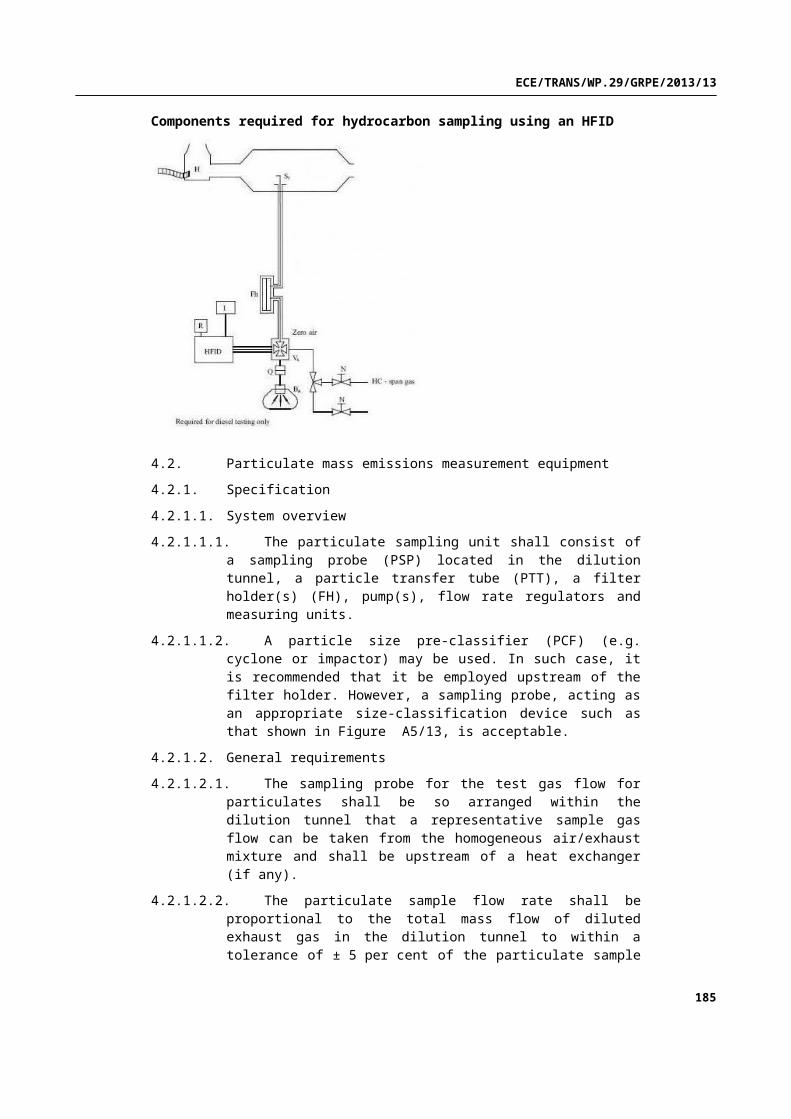
ECE/TRANS/WP.29/GRPE/2013/13
M ri=∑j=1
d
Mrij'
d(2)
M pi={M si × D+M ri× dD+d } (3)
where for each compound (i) considered:
M sij' are the mass emissions of compound (i) over one operating cycle (or
equivalent engine test bench cycle) without regeneration, g/km;
M rij' are the mass emissions of compound (i) over one operating cycle (or
an equivalent engine test bench cycle) during regeneration. (if d>1, the first WLTC test is run cold, and subsequent cycles are hot), g/km;
M si are the mean mass emissions of compound (i) without regeneration, g/km;
M ri are the mean mass emissions of compound (i) during regeneration, g/km;
M pi are the mean mass emissions of compound (i), g/km;
n is the number of test points at which emissions measurements (WLTC operating cycles or equivalent engine test bench cycles) made between two cycles where regenerative phases occur, 2;
d is the number of operating cycles required for regeneration;
D is the number of operating cycles between two cycles where regenerative phases occur.
Figure A6.App1/1Parameters measured during emissions test during and between cycles where regeneration occurs (schematic example, the emissions during D may increase or decrease)
185

ECE/TRANS/WP.29/GRPE/2013/13
3.1.1. Calculation of the regeneration factor K for each compound (i) considered.
The manufacturer may elect to determine for each compound independently either additive offsets or multiplicative factors.
K i factor: K i=M pi
M si
K i offset: K i=M pi−M si
M si, M pi and K i results, and the manufacturer’s choice of type of factor shall be recorded.
K i may be determined following the completion of a single sequence.
3.2. Calculation of combined exhaust emissions of multiple periodic regenerating systems
M sik=∑j=1
nk
M sik , j'
nk
for n j≥ 2 (4)
M rik=∑j=1
dk
M rik , j'
dk
(5)
M si=∑k=1
x
M sik × Dk
∑k=1
x
Dk
(6)
186
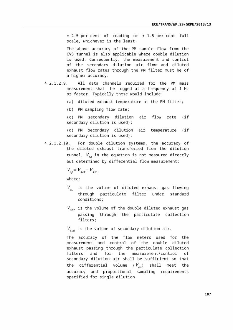
ECE/TRANS/WP.29/GRPE/2013/13
M ri=∑k=1
x
Mrik × dk
∑k=1
x
dk
(7)
M pi=M si ×∑
k=1
x
D k+M ri ×∑k=1
x
dk
∑k=1
x
( Dk+dk )(8)
M pi=∑k=1
x
( M sik × Dk+M rik × dk )
∑k=1
x
( Dk+dk )(9)
K i factor: K i=M pi
M si
K i offset: K i=M pi−M si
where:
M si are the mean mass emissions of all events k of compound (i), without regeneration, g/km;
M ri are the mean mass emissions of all events k of compound (i) during regeneration, g/km;
M pi are the mean mass emission of all events k of compound (i), g/km;
M sik are the mean mass emissions of event k of compound (i), without regeneration, g/km;
M rik are the mean mass emissions of event k of compound (i) during regeneration, g/km;
M sik , j'
are the mass emissions of event k of compound (i) in g/km over one Type 1 operating cycle (or equivalent engine test bench cycle) without regeneration measured at point j; 1 ≤ j≤ nk , g/km;
M rik , j' are the mass emissions of event k of compound (i) over one Type 1
operating cycle (or equivalent engine test bench cycle) during regeneration (when j>1, the first Type 1 test is run cold, and subsequent cycles are hot) measured at operating cycle j where 1≤ j≤ dk, g/km;
nk are the number of test points of event k at which emissions measurements (Type 1 operating cycles or equivalent engine test bench cycles) are made between two cycles where regenerative phases occur, 2;
187
ECE/TRANS/WP.29/GRPE/2013/13
dk is the number of operating cycles of event k required for regeneration;
Dk is the number of operating cycles of event k between two cycles where regenerative phases occur;
x is the event number.
188

ECE/TRANS/WP.29/GRPE/2013/13
Figure A6.App1/2Parameters measured during emissions test during and between cycles where regeneration occurs (schematic example)
An example of a system consisting of a particulate trap (DPF) and a NOx
storage trap (DeNOx) is shown below.
DPF: regenerative, equidistant events, similar emissions (± 15per cent) from event to event
189

ECE/TRANS/WP.29/GRPE/2013/13
Dk=Dk+1=D1
dk=dk+1=d1
M rik−M sik=M rik −1−M sik+1
nk=n
DeNOx: A desulphurization (SO2 removal) event is initiated before an influence of sulphur on emissions is detectable (± 15 per cent of measured emissions) and in this example for exothermic reason together with the last DPF regeneration event performed.
M sik , j=1' =constant
M sik=M sik+1=M si 2
M rik=Mrik+1=M ri 2
For SO2 removal event:
M ri2 , M si2 , d2 , D2 , n2=1
For a complete DPF + DeNOx system:
M si=n × M si 1× D 1+M si 2× D2
n × D 1+D2
M ri=n× M ri1 ×d1+M ri2 ×d2
n ×d1+d2
M pi=M si+M ri
n× ( D1+d1 )+D2+d2
=n× ( M si1 × D1+M ri1 × d1 )+M si2× D2+M ri2 ×d2
n× ( D1+d1 )+D2+d2
The calculation of K i for multiple periodic regenerating systems is only possible after a certain number of regeneration phases for each system.
After performing the complete procedure (A to B, see Figure A6.App1/2), the original starting conditions A should be reached again.
190

ECE/TRANS/WP.29/GRPE/2013/13
Annex 6 - Appendix 2
Test procedure for electric power supply system monitoring
1. General
This Appendix defines the specific provisions regarding the correction of test results for fuel consumption (l/100 km) and CO2 emissions (g/km) as a function of the energy balance ΔE REESS for the vehicle batteries.
The corrected values for fuel consumption and CO2 emissions should correspond to a zero energy balance (ΔE REESS=0), and are calculated using a correction coefficient determined as defined below.
2. Measurement equipment and instrumentation
2.1. Current transducer
2.1.1. The battery current shall be measured during the tests using a clamp-on or closed type current transducer. The current transducer (i.e. a current sensor without data acquisition equipment) shall have a minimum accuracy of 0.5 per cent of the measured value (in A) or 0.1 per cent of full scale deflection.
2.1.2. The current transducer shall be fitted on one of the cables connected directly to the battery. In order to easily measure battery current using external measuring equipment, manufacturers should preferably integrate appropriate, safe and accessible connection points in the vehicle. If this is not feasible, the manufacturer shall support the responsible authority by providing the means to connect a current transducer to the battery cables in the above described manner.
2.1.3. Current transducer output shall be sampled with a minimum frequency of 5 Hz. The measured current shall be integrated over time, yielding the measured value of Q, expressed in ampere-hours (Ah).
2.2. Vehicle on-board data
2.2.1. Alternatively during the tests the battery current shall be determined using vehicle- based data. In order to use this measurement method, the following information shall be accessible from the test vehicle:
(a) integrated charging balance value since last ignition run in Ah;
(b) integrated on-board data charging balance value calculated with a minimum sample frequency of 5 Hz;
(c) the charging balance value via an OBD connector as described in SAE J1962.
2.2.2. The accuracy of the vehicle on-board battery charging and discharging data shall be demonstrated by the manufacturer.
The manufacturer may create a vehicle family to prove that the vehicle on-board battery charging and discharging data are correct. The accuracy of the data shall be demonstrated on a representative vehicle.
The following family criteria shall be valid:
191

ECE/TRANS/WP.29/GRPE/2013/13
(a) identical combustion processes;
(b) identical charge and/or recuperation strategy (software battery data module);
(c) on-board data availability;
(d) identical charging balance measured by battery data module;
(e) identical on-board charging balance simulation.
3. Measurement procedure
3.1. External battery charging
Before the preconditioning test cycle, the battery shall be fully charged. The battery shall not be charged again before the official testing according to paragraph 1.2.6.2. of this Annex.
3.2. Measurement of the battery current shall start at the same time as the test starts and shall end immediately after the vehicle has driven the complete driving cycle.
3.3. The electricity balance, Q, measured in the electric power supply system, is used as a measure of the difference in the vehicle REESS’s energy content at the end of the cycle compared to the beginning of the cycle. The electricity balance is to be determined for the total WLTC for the applicable vehicle class.
3.4. Separate values of Qphase shall be logged over the cycle phases required to be driven for the applicable vehicle class.
3.5. Test results CO2 ,CS and FCCS are corrected as a function of the REESS energy balance RCB.
3.6. The test results shall be the uncorrected measured values of CO2 ,CS and FCCS in case any of the following applies:
(a) the manufacturer can prove that there is no relation between the energy balance and fuel consumption;
(b) ΔE REESS as calculated from the test result corresponds to REESS charging;
(c) ΔE REESS as calculated from the test result corresponds to REESS charging and discharging. ΔE REESS, expressed as a percentage of the energy content of the fuel consumed over the cycle, is calculated in the equation below:
ΔE REESS=0.0036 × RCB × UREESS
EFuel×100
where:
ΔE REESS is the change in the REESS energy content, per cent;
U REESS is the nominal REESS voltage, V;
RCB is REESS charging balance over the whole cycle, Ah;
192

ECE/TRANS/WP.29/GRPE/2013/13
EFuel is the energy content of the consumed fuel, Wh.
ΔE REESS is lower than the RCB correction criteria, according to the equation below and Table 1:
ΔE REESS ≤ RCB correctioncriteria
Table A6.App2/1RCB correction criteria
CycleWLTC city (low + me-dium)
WLTC (low + medium + high)
WLTC (low + medium + high + extra high)
RCB correction criteria (%)
1.5 1 0.5
4. Correction Method
4.1. To apply the correction function, the electric power to the battery must be calculated from the measured current and the nominal voltage value for each phase of the WLTC test:
∆ E el− phase(i)=U REESS × ∫0
t−end
I (t )phase(i )× dt
where:
∆ Eel−phase( i) is the change in the electrical REESS energy content of phase i, MJ;
U REESS is the nominal REESS voltage, V;
I (t)phase(i) is the electric current in phase (i), A;
t−end is the time at the end of phase (i), seconds (s).
4.2. For correction of fuel consumption, l/100 km, and CO2 emissions, g/km, test results as a function of the energy balance of the electric power supply system battery, combustion process-dependent Willans factors from Table A6.App2/2 (paragraph 4.8. below) must be used.
4.3. The resulting fuel consumption difference of the engine for each WLTC phase due to load behaviour of the alternator for charging a battery shall be calculated as shown below:
∆ FC phase(i )=∆ Eel−phase(i)×1
ηalternator× Willansfactor
where:
∆ FC phase(i ) is the resulting fuel consumption difference of phase (i), l;
∆ Eel−phase( i) is the change in the electrical REESS energy content of phase (i), MJ;
ηalternator is the efficiency of the alternator;
Willans factor is the combustion process specific Willans factor.
193

ECE/TRANS/WP.29/GRPE/2013/13
4.4. The resulting CO2 emissions difference of the engine for each WLTC phase due to load behaviour of the alternator for charging a battery shall be calculated as shown below:
∆ CO2 , phase(i)=∆ Eel−phase (i )×1
ηalternator×Willans factor
where:
∆ CO2 , phase(i) is the resulting CO2-emission difference of phase (i), g;
∆ Eel−phase( i) is the change in the electrical REESS energy content of phase (i), MJ;
ηalternator is the efficiency of the alternator;
Willans factor is the combustion process specific Willans factor.
4.5. For this specific calculation, a fixed electric power supply system alternator efficiency shall be used:
ηalternator=0.67 for electric power supply systembattery alternators
4.6. The consumption difference of the engine for the WLTC test is the sum over the (i) single phases as shown below:
∆ FC cycle=∑i=1
n
∆ FC phase(i )
where:
∆ FC cycle is the change in consumption over the whole cycle, l.
4.7. The CO2 emissions difference of the engine for the WLTC test is the sum over the (i) single phases as shown below:
∆ CO2 ,cycle=∑i=1
n
∆ CO2 , phase(i)
where:
∆ CO2 ,cycle is the change in CO2-emission over the whole cycle, g.
4.8. For correction of the fuel consumption, l/100 km, and CO2 emission, g/km, the values contained in Table A6.App2/2 shall be used.
Table A6.App2/2Correction of the fuel consumption and CO2 emission
Self-induced
Charged
Posit-ive ig-
Ga
l/k
0.
0.
194

ECE/TRANS/WP.29/GRPE/2013/13
Self-induced
Charged
nition sol-ine (E0)
Wh
264
28
gCO2/kWh
630
668
Gasol-ine (E5)
l/kWh
0.268
0.284
gCO2/kWh
628
666
CNG (G20)
m³/kWh
0.259
0.275
gCO2/kWh
465
493
LPG
l/kWh
0.342
0.363
gCO2/k
557
591
195

ECE/TRANS/WP.29/GRPE/2013/13
Self-induced
Charged
Wh
E85
l/kWh
0.367
0.389
gCO2/kWh
608
645
Com-pres-sion igni-tion
Diesel (B0)
l/kWh
0.22
0.22
gCO2/kWh
581
581
Diesel (B5)
l/kWh
0.22
0.22
gCO2/kWh
581
581
196

ECE/TRANS/WP.29/GRPE/2013/13
Annex 7
Calculations
1. General requirements
1.1. Calculations related specifically to hybrid and pure electric vehicles are described of Annex 8.
1.2. The calculations described in this Annex shall be used for vehicles using combustion engines.
1.3. . The final test result shall be rounded in one step to the number of places to the right of the decimal point indicated by the applicable emission standard plus one additional significant figure. Intermediate steps in the calculations shall not be rounded.
1.4. . The NOx correction factor, KH , shall be rounded to 2 decimal places.
1.5. . The dilution factor, DF , shall be rounded to 2 decimal places.
1.6. . For information not related to standards, good engineering judgement shall be used.
2. Determination of diluted exhaust gas volume
2.1. Diluted exhaust volume calculation for a variable dilution device capable of operating at a constant or variable flow rate.
2.1.1. The parameters showing the volumetric flow shall be recorded continuously. The total volume shall be recorded for the duration of the test.
2.2. Volume calculation for a variable dilution device using a positive displacement pump
2.2.1. The volume shall be calculated using the following equation:
V=V 0× N (1)
where:
V is the volume of the diluted gas, in litres per test (prior to correction);
V 0 is the volume of gas delivered by the positive displacement pump in testing conditions, N-1;
N is the number of revolutions per test.
2.2.1.1. Correcting the volume to standard conditions
2.2.1.1.1. The diluted exhaust gas volume is corrected to standard conditions according to the following equation:
V mix=V × K1×( PB−P1
T p) (2)
where:
197

ECE/TRANS/WP.29/GRPE/2013/13
K 1=273.15(K )
101.325(kPa)=2.6961
PB is the test room barometric pressure, kPa;
P1 is the vacuum at the inlet to the positive displacement pump relative to the ambient barometric pressure, kPa;
T p is the average temperature of the diluted exhaust gas entering the positive displacement pump during the test, degrees Kelvin (K).
3. Mass emissions
3.1. General requirements
3.1.1. Assuming no compressibility effects, all gases involved in the engine intake/combustion/exhaust process can be considered to be ideal according to Avogadro’s hypothesis.
3.1.2. The mass M of gaseous compounds emitted by the vehicle during the test shall be determined by obtaining the product of the volumetric concentration of the gas in question and the volume of the diluted exhaust gas with due regard for the following densities under the reference conditions of 101.325 kPa and 273.15 K:
Carbon monoxide (CO) ρ=1.25 g/l
Carbon dioxide (CO2) ρ=1.964 g/l
Hydrocarbons:
for petrol (E0) (C1H1.85) ρ=0.619 g/1
for petrol (E5) (C1H1.89O0.016) ρ=0.631 g/1
for diesel (B0) (C1Hl.86) ρ=0.619 g/1
for diesel (B5) (C1Hl.86O0.005) ρ=0.622 g/1
for LPG (CH2.525) ρ=0.649 g/l
for NG/biomethane (C1H4) ρ=0.714 g/l
for ethanol (E85) (C1H2,74O0.385) ρ=0.932 g/l
Nitrogen oxides (NOx) ρ=2.05 g/1
Nitrogen dioxide (NO2) ρ=2.05 g/1
Nitrous oxide (N2O) ρ=1.964 g/1
The density for NMHC mass calculations shall be equal to that of total hydrocarbons at 273.15 K and 101.325 kPa and is fuel dependent.
3.2. Mass emissions calculation
3.2.1. Mass emissions of gaseous compounds shall be calculated using the following equation:
198

ECE/TRANS/WP.29/GRPE/2013/13
M i=V mix × ρi × KH × Ci ×10−6
d(3)
where:
M i is the mass emissions of compound (i), g/km;
V mix is the volume of the diluted exhaust gas expressed in litres per test and corrected to standard conditions (273.15 K and 101.325 kPa);
ρi is the density of compound (i) in grams per litre at normal temperature and pressure (273.15 K and 101.325 kPa);
KH is a humidity correction factor applicable only to the mass emissions of oxides of nitrogen (NO2 and NOx);
C i is the concentration of compound (i) in the diluted exhaust gas expressed in ppm and corrected by the amount of the compound (i) contained in the dilution air;
d is the distance driven over the corresponding WLTC , km.
3.2.1.1. The concentration of a gaseous compound in the diluted exhaust gas shall be corrected by the amount of the gaseous compound in the dilution air as follows:
C i=C e−Cd ×(1− 1DF ) (4)
where:
C i is the concentration of gaseous compound (i) in the diluted exhaust gas corrected by the amount of (i) contained in the dilution air, ppm;
C e is the measured concentration of gaseous compound (i) in the diluted exhaust gas, ppm;
Cd is the concentration of gaseous compound (i) in the air used for dilution, ppm;
DF is the dilution factor.
3.2.1.1.1. The dilution factor, DF , is calculated as follows:
DF= 13.4CCO2+(CHC+CCO) × 10−4 for petrol (E5)
(5a)
DF= 13.5CCO2+(CHC+CCO) × 10−4 for diesel (B5)
(5b)
DF= 11.9CCO2+(CHC+CCO) × 10−4 for LPG
(5c)
199

ECE/TRANS/WP.29/GRPE/2013/13
DF= 9.5CCO2+(CHC+CCO) × 10−4 for NG/biomethane
(5d)
DF= 12.5CCO2+(CHC+CCO) × 10−4 for ethanol (E85)
(5e)
3.2.1.1.2. General equation for the dilution factor (DF) for each reference fuel with an average composition of CxHyOz is:
DF= XCCO2+(CHC+CCO) × 10−4 (6)
X=100 × x
x+ y2+3.76 (x+ y
4− z
2 )where:
CCO2 is the concentration of CO2 in the diluted exhaust gas contained in the sampling bag, per cent volume;
CHC is the concentration of HC in the diluted exhaust gas contained in the sampling bag, ppm carbon equivalent;
CCO is the concentration of CO in the diluted exhaust gas contained in the sampling bag, ppm.
3.2.1.1.3. Methane measurement3.2.1.1.3.1. For methane measurement using a GC-FID, NMHC is
calculated as follows:CNMHC=CTHC−( Rf CH 4 ×CCH 4 ) (7)where:CNMHC is the corrected concentration of NMHC in the
diluted exhaust gas, ppm carbon equivalent;CTHC is the concentration of THC in the diluted exhaust
gas, ppm carbon equivalent and corrected by the amount of THC contained in the dilution air;
CCH 4 is the concentration of CH4 in the diluted exhaust gas, ppm carbon equivalent and corrected by the amount of CH4 contained in the dilution air;
Rf CH 4 is the FID response factor to methane as defined in paragraph 5.4.3.2. of Annex 5.
3.2.1.1.3.2. For methane measurement using a NMC-FID, the calculation of NMHC depends on the calibration gas/method used for the zero/calibration adjustment.
200

ECE/TRANS/WP.29/GRPE/2013/13
The FID used for the THC measurement (without NMC) shall be calibrated with propane/air in the normal manner.
For the calibration of the FID in series with NMC, the following methods are permitted :
(a) the calibration gas consisting of propane/air bypasses the NMC;
(b) the calibration gas consisting of methane/air passes through the NMC.
It is strongly recommended to calibrate the methane FID with methane/air through the NMC.
In case (a), the concentration of CH4 and NMHC shall be calculated as follows:
CCH 4=CHC ( w/NMC )−CHC ( w/oNMC ) × (1−EE )
r h× ( EE−EM )(8)
CNMHC=C HC ( w/oNMC ) × ( 1−EM )−CHC ( w/NMC )
EE−EM
(9)
In case (b), the concentration of CH4 and NMHC shall be calculated as follows:
CCH 4=CHC ( w/NMC ) × rh × (1−EM )−CHC (w /oNMC ) × (1−EE )
rh× ( EE−EM )(10)
CNMHC=C HC ( w/oNMC ) × ( 1−EM )−CHC ( w/NMC ) ×rh × (1−EM )
EE−EM
(11)
where:
CHC ( w/NMC ) is the HC concentration with sample gas flowing through the NMC, ppm C;
CHC ( w/oNMC ) is the HC concentration with sample gas bypassing the NMC, ppm C;
rh is the methane response factor as determined per paragraph 5.4.3.2 of Annex 5;
EM is the methane efficiency as determined per paragraph 3.2.1.1.3.3.1. . below;
EE is the ethane efficiency as determined per paragraph 3.2.1.1.3.3.2. . below.
If rh < 1.05, it may be omitted in equations 8, 10 and 11.
3.2.1.1.3.3. Conversion efficiencies of the non-methane cutter (NMC)
The NMC is used for the removal of the non-methane hydrocarbons from the sample gas by oxidizing all hydrocarbons except methane. Ideally, the conversion for methane is 0 per cent, and for the other hydrocarbons represented by ethane is 100 per cent. For the accurate measurement of
201

ECE/TRANS/WP.29/GRPE/2013/13
NMHC, the two efficiencies shall be determined and used for the calculation of the NMHC emission.
3.2.1.1.3.3.1. . Methane conversion efficiency
The methane/air calibration gas shall be flowed to the FID through the NMC and bypassing the NMC and the two concentrations recorded. The efficiency shall be determined as follows:
EM=1−C HC ( w/NMC )
CHC ( w/oNMC )(12)
where:
CHC ( w/NMC ) is the HC concentration with CH4 flowing through the NMC, ppm C;
CHC ( w/oNMC ) is the HC concentration with CH4 bypassing the NMC, ppm C.
3.2.1.1.3.3.2. . Ethane conversion efficiency
The ethane/air calibration gas shall be flowed to the FID through the NMC and bypassing the NMC and the two concentrations recorded. The efficiency shall be determined as follows:
EE=1−CHC (w /NMC )
C HC ( w/oNMC )(13)
where:
CHC ( w/NMC ) is the HC concentration with C2H6 flowing through the NMC, ppm C;
CHC ( w/oNMC ) is the HC concentration with C2H6 bypassing the NMC in ppm C.
If the ethane conversion efficiency of the NMC is 0.98 or above, EE shall be set to 1 for any subsequent calculation.
3.2.1.1.3.4. If the methane FID is calibrated through the cutter, then EM is 0.
Equation (10) from above becomes:
CCH 4=CHC (w /NMC ) (14)
Equation (11) from above becomes:
CNMHC=CHC (w /oNMC )−CHC ( w/ NMC ) ×rh (15)
The density used for NMHC mass calculations shall be equal to that of total hydrocarbons at 273.15 K and 101.325 kPa and is fuel dependent.
3.2.1.1.4. Flow weighted average concentration calculation
When the CVS flow rate qVCVS over the test varies more than ± 3 per cent of the average flow rate, a flow weighted average shall be used for all continuous diluted measurements including PN:
202

ECE/TRANS/WP.29/GRPE/2013/13
C e=∑i=1
n
qVCVS(i)× ∆ t × C(i)
V(16)
where:
C e is the flow-weighted average concentration;
qVCVS(i) is the CVS flow rate at time t=i× ∆ t , m³/min;
C (i) is the concentration at time t=i× ∆ t , ppm;
∆ t sampling interval, seconds (s);
V total CVS volume, m³.
3.2.1.2. Calculation of the NOx humidity correction factor
In order to correct the influence of humidity on the results of oxides of nitrogen, the following calculations apply:
KH= 11−0.0329 × ( H a−10.71 ) (17)
where:
H a=6.211× Ra× Pd
PB−Pd × Ra× 10−2 (18)
and:
H a is the absolute humidity, grams of water per kilogram of dry air;
Ra is the relative humidity of the ambient air, per cent;
Pd is the saturation vapour pressure at ambient temperature, kPa;
PB is the atmospheric pressure in the room, kPa.
The KH factor shall be calculated for each phase of the test cycle.
The ambient temperature and relative humidity shall be defined as the average of the continuously measured values during each phase.
3.2.1.3. Determination of NO2 concentration from NO and NOx
NO2 is determined by the difference between NOx concentration from the bag corrected for dilution air concentration and NO concentration from continuous measurement corrected for dilution air concentration
3.2.1.3.1. NO concentrations
3.2.1.3.1.1. NO concentrations shall be calculated from the integrated NO analyser reading, corrected for varying flow if necessary.
3.2.1.3.1.2. The average NO concentration is calculated as follows:
203

ECE/TRANS/WP.29/GRPE/2013/13
C e=∫t1
t2
CNO . dt
t2−t 1
(19)
where:
∫t1
t2
CNO dt is the integral of the recording of the modal NO analyser over
the test (t2-t1);
C e is the concentration of NO measured in the diluted exhaust, ppm;
3.2.1.3.1.3. Dilution air concentration of NO is determined from the dilution air bag. Correction is carried out according to section 3.2.1.1. of this Annex.
3.2.1.3.2. NO2 concentrations
3.2.1.3.2.1. Determination NO2 concentration from direct diluted measurement
3.2.1.3.2.2. NO2 concentrations shall be calculated from the integrated NO2 analyser reading, corrected for varying flow if necessary.
3.2.1.3.2.3. The average NO2 concentration is calculated as follows:
C e=∫t1
t2
CNO2.dt
t 2−t 1
(20)
where:
∫t1
t2
CNO2. dt
is the integral of the recording of the modal NO2 analyser over
the test (t2-t1);
C e is the concentration of NO2 measured in the diluted exhaust, ppm.
3.2.1.3.2.4. Dilution air concentration of NO2 is determined from the dilution air bags. Correction is carried out according to section 3.2.1.1. of this Annex.
3.2.2. Determination of the HC mass emissions from compression-ignition engines
3.2.2.1. To calculate HC mass emission for compression-ignition engines, the average HC concentration is calculated as follows:
C e=∫t1
t2
CHC . dt
t2−t1
(21)
where:
204

ECE/TRANS/WP.29/GRPE/2013/13
∫t1
t2
CHC is the integral of the recording of the heated FID over the test
(t1 to t2);
C e is the concentration of HC measured in the diluted exhaust in ppm of C i and is substituted for CHC in all relevant equations.
3.2.2.1.1. Dilution air concentration of HC shall be determined from the dilution air bags. Correction shall be carried out according to section 3.2.1.1. of this Annex.
3.2.3. CO2 calculation for individual vehicles in a CO2 vehicle family
3.2.3.1. CO2 emissions without using the interpolation method
If the road load and emissions have been not been measured on test vehicle L in addition to test vehicle H, the value M CO2
, as calculated in section 3.2.1. above, shall be attributed to all individual vehicles in the CO 2 vehicle family and the CO2 interpolation method is not applicable.
3.2.3.2. CO2 emissions using the interpolation method
If the road load and emissions are measured on test vehicles L and H, the CO2
emission for each individual vehicle in the CO2 vehicle family may be calculated according to the CO2 interpolation method outlined in the following paragraphs.
3.2.3.2.1. Determination of CO2 emissions test vehicles L and H
The mass of CO2 emissions, M CO2, for test vehicles L and H shall be
determined according to the calculation in section 3.2.1. above for the individual cycle phases p applicable for the class of the CO2 vehicle family. and are referred to as M CO2−L, p and M CO2−H , p respectively.
3.2.3.2.2. Road load calculation for an individual vehicle
3.2.3.2.2.1. Mass of the individual vehicle
The selected test masses TML and TMH as determined in paragraph 4.2.1.3.1. of Annex 4 shall be used as input for the interpolation method.
The mass of the optional equipment mo shall be calculated for the individual vehicle according to the following equation:
mo=∑i=1
n
∆ mi (22)
where:
mo is the difference in mass between the individual vehicle and TM L;
∆ mi is the mass of an individual option i on the vehicle (∆ mi is positive for an option that adds mass with respect to TM L and vice versa);
n is the number of options that are different between the individual vehicle and test vehicle L.
205

ECE/TRANS/WP.29/GRPE/2013/13
The value of mo for test vehicle H shall be the same as the difference between TM H and TM L.
The mass of the individual vehicle is calculated according to the following equation:
TM ind=TM L+mo (23)
where TM ind is the mass of the individual vehicle used as input for the CO 2
interpolation method.
If the same test mass was used for test vehicles L and H, the value of TM ind shall be set to TM H for the interpolation method.
3.2.3.2.2.2. Rolling resistance of the individual vehicle
According to paragraph 4.2.2.1. of Annex 4, the actual rolling resistance values for the selected tyres on test vehicle L, RRL, and test vehicle H, RRH, shall be used as input for the interpolation method.
For the tyres fitted to the individual vehicle, the value of the rolling resistance RRind shall be set to the class value of the applicable tyre rolling resistance class, according to Table A4/1 of Annex 4.
If the same tyres were fitted to test vehicles L and H, the value of RRind for the interpolation method shall be set to RR H
3.2.3.2.2.3 Aerodynamic drag of the individual vehicle
The aerodynamic drag shall be measured for each of the drag influencing options at a certified wind tunnel fulfilling the requirements of section 3.2. of Annex 4.
The aerodynamic drag of options on the exterior of the individual vehicle shall be calculated according to the following equation:
∆ [Cd × A f ]ind=∑i=1
n
∆ [Cd × A f ]i (24)
where:
Cd is the aerodynamic drag coefficient;
A f is the frontal area of the vehicle, m2;
∆ [Cd × A f ]ind is the difference in aerodynamic drag between the individual vehicle and the test vehicle L, due to options on the vehicle that differ from those installed on the test vehicle L, m2;
∆ [Cd × A f ]i is the aerodynamic drag difference by an individual feature i on
the vehicle (∆ [Cd × A f ]i is positive for an option that adds aerodynamic drag with respect to test vehicle L and vice versa), m2;
n is the number of options on the vehicle that are different between the individual and the test vehicle L.
206

ECE/TRANS/WP.29/GRPE/2013/13
The sum of all ∆ [Cd × A f ]i between options installed on the test vehicles L and H shall correspond to the total difference between the Cd × A f values for the test vehicles L and H, referred to as ∆ [Cd × A f ] LH.
The sum of all ∆ [Cd × A f ]i, expressed as Δf 2, between options installed on the test vehicles L and H shall correspond to the difference in f 2 between the test vehicles L and H.
If the same options on the vehicle were also installed on test vehicles L and H, the value of ∆ [Cd × A f ]ind for the interpolation method shall be set to zero.
3.2.3.2.2.4. Calculation of road load for individual vehicles in the CO2 vehicle family
The road load coefficients f 0, f 1 and f 2 (as defined of Annex 4) for the test vehicles H and L are referred to as f 0 , H, f 1 ,H and f 2 , H and f 0 , L, f 1 ,L and f 2 , L respectively. An adjusted road load curve for the test vehicle L is defined as follows:
FL (v )=f 0 , L¿ + f 1 , H . v+ f 2 , L
¿ . v2 (25)
Applying the least squares regression method, adjusted road load coefficients f 0 , L
¿ and f 2 , L¿ shall be determined for FL (v ) with the linear coefficient f 1 ,L
¿ set to f 1 ,H . The road load coefficients f 0 ,ind, f 1 ,ind and f 2 ,ind for the individual vehicle in the CO2 vehicle family are calculated as follows:
f 0 ,ind=f 0 , H−∆ f 0 ×(TM H × RRH −TM ind × RRind )
(TM H × RRH−TM L× RR L)(26)
or, if (TM H × RR H−TM L × RRL) = 0,
f 0 ,ind=f 0 , H−∆ f 0 (27)
f 1 ,ind=f 1 , H (28)
f 2 ,∈d= f 2 , H−∆ f 2(∆ [Cd× Af ]LH−∆ [Cd × A f ]ind )
(∆ [Cd × A f ]LH )(29)
or, if ∆ [Cd × A f ] LH = 0,
f 2 ,ind=f 2 , H−∆ f 2 (30)
where:
∆ f 0= f 0 , H−f 0 , L¿ (31)
∆ f 2= f 2 , H− f 2 ,L¿ (32)
3.2.3.2.2.5. Calculation of cycle energy per phase
The cycle energy demand Ek , p and distance dc , p per cycle phase p applicable for that vehicle shall be calculated according to the procedure in section 5. of this Annex, for the following sets k of road load coefficients and masses:
207

ECE/TRANS/WP.29/GRPE/2013/13
k=1: f 0=f 0 , L¿ , f 1=f 1 , H , f 2=f 2 , L
¿ ,m=TM L (33)
(test vehicle L)
k=2: f 0= f 0 , H¿ , f 1= f 1 , H , f 2=f 2 , H
¿ , m=TM H (34)
(test vehicle H)
k=3: f 0=f 0 ,ind , f 1=f 1 , H , f 2=f 2 ,ind¿ ,m=TM ind (35)
(individual vehicle in the CO2 vehicle family)
3.2.3.2.2.6. Calculation of the CO2 value for an individual vehicle by the CO2
interpolation method
For each cycle phase p applicable for that class vehicle in a CO2 vehicle family, the contribution to the total mass of CO2 for the individual vehicle shall be calculated as follows:
M CO2 −ind , p=M CO2−L, p+( E3 , p−E1 , p
E2 , p−E1 , p)× ( M CO2−H , p−M CO2−L , p ) (36)
The CO2 mass emissions attributed to the individual vehicle of the CO2
vehicle family MCO2-ind shall be calculated by the following equation:
M CO2−ind=∑
pM CO2−ind , p× dc , p
∑p
dc , p
(37)
for all of the applicable cycle phases p.
3.3. Mass of particulate emissions
3.3.1. Particulate emission M p (g/km) is calculated as follows:
M p=(V mix+V ep) × Pe
V ep × d(38)
where exhaust gases are vented outside tunnel;
and:
M p=V mix × Pe
V ep ×d(39)
where exhaust gases are returned to the tunnel;
where:
V mix is the volume of diluted exhaust gases (see section 2. of this Annex), under standard conditions;
V ep is the volume of diluted exhaust gas flowing through the particulate filter under standard conditions;
Pe is the particulate mass collected by one or more filters;
d distance corresponding to the operating cycle, km;
208

ECE/TRANS/WP.29/GRPE/2013/13
M p is the particulate emission, g/km.
3.3.1.1. Where correction for the particulate background level from the dilution system has been used, this shall be determined in accordance with section 1.2.1.3.1. of Annex 6. In this case, the particulate mass (g/km) shall be calculated as follows:
M p={ P e
V ep−[ Pa
V ap×(1− 1
DF )]}×(V mix+V ep)
d (40)
in the case where exhaust gases are vented outside tunnel;
M p={ P e
V ep−[ Pa
V ap×(1− 1
DF )]}×(V mix )
d(41)
in the case where exhaust gases are returned to the tunnel;
where:
V ap is the volume of tunnel air flowing through the background particulate filter under standard conditions;
Pa is the rolling average of the particulate mass collected from the dilution tunnel as specified in this GTR up to a maximum equivalent of 1mg/km at the equivalent CVS and particulate sampling flow rates;
DF is the dilution factor determined in paragraph 3.2.1.1.1. of this Annex.
Where application of a background correction results in a negative particulate mass (in g/km), the result shall be considered to be zero g/km particulate mass.
3.3.2. Calculation of particulate mass emissions using the double dilution method
V ep=V set−V ssd (42)
where:
V ep is the volume of diluted exhaust gas flowing through the particulate filter under standard conditions;
V set is the volume of the double diluted exhaust gas passing through the particulate collection filters;
V ssd is the volume of the secondary dilution air.
Where the secondary diluted PM sample gas is not returned to the tunnel, the CVS volume shall be calculated as in single dilution, i.e.:
V mix=V mix indicated+V ep (43)
where V mix indicated is the measured volume of diluted exhaust gas in the dilution system following extraction of particulate sample under standard conditions.
4. Determination of particle numbers
4.1. Number emission of particles shall be calculated by means of the following equation:
209
ECE/TRANS/WP.29/GRPE/2013/13
N=V ×k × (C s× f r−Cb× f rb ) ×103
d(44)
where:
N is the particle number emission, particles per kilometre;
V is the volume of the diluted exhaust gas in litres per test (after primary dilution only in the case of double dilution) and corrected to standard conditions (273.15 K and 101.325 kPa);
k is a calibration factor to correct the particle number counter measurements to the level of the reference instrument where this is not applied internally within the particle number counter. Where the calibration factor is applied internally within the particle number counter, the calibration factor shall be 1;
C s is the corrected concentration of particles from the diluted exhaust gas expressed as the average number of particles per cubic centimetre figure from the emissions test including the full duration of the drive cycle. If the volumetric mean concentration results (C) from the particle number counter are not output at standard conditions
(273.15 K and 101.325 kPa), the concentrations shall be corrected to those conditions (C s);
Cb is either the dilution air or the dilution tunnel background particle concentration, as permitted by the responsible authority, in
particles per cubic centimeter, corrected for coincidence and to standard conditions (273.15 K and 101.325 kPa);
f r is the mean particle concentration reduction factor of the volatile particle remover at the dilution setting used for the test;
f rb is the mean particle concentration reduction factor of the volatile particle remover at the dilution setting used for the background measurement;
d is the distance corresponding to the operating cycle, km
C shall be calculated from the following equation:
C=∑i=1
n
Ci
n(45)
where:
C i is a discrete measurement of particle concentration in the diluted gas exhaust from the particle counter; particles per cubic centimetre and corrected for coincidence;
n is the total number of discrete particle concentration measurements made during the operating cycle and shall be calculated using the following equation:
210

ECE/TRANS/WP.29/GRPE/2013/13
n=T × f (46)
where:
T is the time duration of the operating cycle, s;
f is the data logging frequency of the particle counter, Hz.
5. Calculation of cycle energy demand
Basis of the calculation is the target speed trace given in discrete time sample points t i between t start and t end. In case of the class 2 and class 3 cycles t start=0 s and t end=1800 s. For a specific cycle phase, t start and t end shall be taken from Annex 1.
For the calculation, each time sample point is interpreted as time period. The duration ∆t of these periods depends on the sampling frequency (1 s for 1 Hz, 0.5 s for 2 Hz or 0.1 s for 10 Hz).
The total energy demand E for the whole cycle or a specific cycle phase shall be calculated by summing Ei over the corresponding cycle time between tstart
and tend.
Ei=F i ×d i if F i>0 (47a)
Ei=0 if F i≤ 0 (47b)
where:
Ei is the energy demand during time period (i-1) to (i), Ws;
F i is the driving force during time period (i-1) to (i), N;
d i is the distance travelled during time period (i-1) to (i), m.
F i=f 0+ f 1 ×( v i+v i−1
2 )+f 2×( v i+v i−1 )2
4 +(1.03 ×TM )× ai (48)
where:
F i is the driving force during time period (i-1) to (i), N;
vi is the target velocity at time ti km/h;
TM is the test mass, kg;
a i is the acceleration during time period (i-1) to (i), m/s²;
f 0, f 1, f 2 are the road load coefficients for the test mass under consideration (TM L, TM H or TM ind) in N, N/km/h and in N/(km/h)² respectively.
d i=( v i+v i−1 )2×3.6
× ( ti−t i−1 ) (49)
where:
d i is the distance travelled in time period (i-1) to (i), m;
211

ECE/TRANS/WP.29/GRPE/2013/13
vi is the target velocity at time t i, km/h;
t i is time, s.
a i=vi−v i−1
3.6 × (ti−ti−1 )(50)
where:
a i is the acceleration during time period (i-1) to (i), m/s²;
vi is the target velocity at time t i, km/h;
t i is time, s.
6. Calculation of fuel consumption
6.1. The fuel characteristics required for the calculation of fuel consumption values shall be taken from Annex 3 in this Regulation.
6.2. The fuel consumption values shall be calculated from the emissions of hydrocarbons, carbon monoxide, and carbon dioxide determined from the measurement results using the provisions defined in this Regulation.
6.3. For a vehicle with a positive ignition engine fuelled with petrol (E5)
FC=( 0.118ρ )× [ (0.848 × HC )+(0.429 ×CO )+(0.273 ×CO2 ) ]
6.4. For a vehicle with a positive ignition engine fuelled with LPGFCnorm=( 0.1212
0.538 )× [ (0.825 × HC )+(0.429 ×CO )+(0.273 ×CO2 ) ]
6.4.1. If the composition of the fuel used for the test differs from the com-position that is assumed for the calculation of the normalised consumption, on the manufacturer's request a correction factor cf may be applied, as follows:
FCnorm=( 0.12120.538 )× (cf ) × [ (0.825 × HC )+ (0.429× CO )+( 0.273× CO2 ) ]
The correction factor cf, which may be applied, is determined as follows:cf =0.825+0.0693 × nactualwhere:nactual is the actual H/C ratio of the fuel used
6.5. For a vehicle with a positive ignition engine fuelled with NG/biomethane
FCnorm=( 0.13360.654 )× [ (0.749 × HC )+(0.429 × CO )+(0.273 ×CO2 ) ]
6.6. For a vehicle with a compression engine fuelled with diesel (B5)
212
ECE/TRANS/WP.29/GRPE/2013/13
FC=( 0.116ρ )× [ (0.861 × HC )+(0.429 ×CO )+(0.273 ×CO2 ) ]
6.7. For a vehicle with a positive ignition engine fuelled with ethanol (E85)
FC=( 0.1742ρ )× [ (0.574 × HC )+(0.429 ×CO )+(0.273 ×CO2 )]
where for all equations in section 6:FC is fuel consumption in l/100 km (or m³ per km in the case of natural gas)HC are the measured emissions of hydrocarbons, g/kmCO are the measured emissions of carbon monoxide, g/kmCO2 are the measured emissions of carbon dioxide, g/kmρ is the density of the test fuel
213

ECE/TRANS/WP.29/GRPE/2013/13
Annex 8
Pure and hybrid electric vehicles
1. General requirements
In the case of testing NOVC-HEV and OVC-HEV vehicles, Appendix 3 to this Annex replaces Appendix 2 of Annex 6.
1.1. Energy balance
The energy balance shall be the sum of the changes in the energy content of all systems storing electric energy (∆ EREESS).
1.2. Electric energy consumption and range testing
Parameters, units and accuracy of measurements shall be as in Table A8/1.
Table A8/1Parameters, units and accuracy of measurements
Parameter Units Accuracy Resolution
Electrical energy (1) Wh ± 1 per cent 0.001 Wh (2)
Electrical current A ± 0.3 per cent FSD or ± 1 per cent of reading (3,4)
0.01 A
(1) Equipment: static meter for active energy.(2) AC watt-hour meter, Class 1 according to IEC 62053-21 or equivalent.(3) Whichever is greater.(4) Current integration frequency 10 Hz or more.
1.3. Emission and fuel consumption testing
Parameters, units and accuracy of measurements shall be the same as those required for conventional combustion engine-powered vehicles as found of Annex 5 (test equipment and calibrations).
1.4. Measurement units and presentation of results
The accuracy of measurement units and the presentation of the results shall follow the indications given in Table A8/2.
Table A8/2Accuracy of measurement units and presentation of the results
Parameter Units Communication of test result
AER, AERcity km Rounded to nearest whole number
EAER, EAERcity km Rounded to nearest whole number
RCDA, RCDAcity km Rounded to nearest whole number
RCDC, RCDCcity km Rounded to nearest whole number
Distance km Rounded to nearest whole number;
214

ECE/TRANS/WP.29/GRPE/2013/13
Parameter Units Communication of test result
for calculation purposes: 0.1 km
Electric energy consump-tion
Wh/km Rounded to nearest whole number
NEC Wh Rounded to first decimal place
NEC ratio per cent Rounded to first decimal place
EAC recharge E Wh Rounded to nearest whole number
FC correction factor l/100 km/(Wh/km) Rounded to 4 significant digits
CO2 correction factor g/km/(Wh/km) Rounded to 4 significant digits
Utility factor Rounded to 3 decimal places
1.5. Type 1 test cycles to be driven
1.5.1. Class 3a vehicles shall drive a cycle consisting of a low phase (Low 3), a medium phase (Medium3-1), a high phase (High3-1) and an extra high phase (Extra High3).
1.5.1.1. At the option of the Contracting Party, the Extra High3 phase may be excluded.
1.5.2. Class 3b vehicles shall drive a cycle consisting of a low phase (Low 3) phase, a medium phase (Medium3-2), a high phase (High3-2) and an extra high phase (Extra High3).
1.5.2.1. At the option of the Contracting Party, the Extra High3 phase may be excluded.
1.6. Range tests for OVC-HEVs and PEVs
1.6.1. Class 3a vehicles shall drive a cycle consisting of a low phase (Low3) and a medium phase (Medium3-1).
1.6.2. Class 3b vehicles shall drive a cycle consisting of a low phase (Low 3) and a medium phase (Medium3-2).
1.7. Hybrid and PEVs with manual transmissions shall be driven according to the manufacturer’s instructions, as incorporated in the manufacturer's handbook of production vehicles and indicated by a technical gear shift instrument.
2. REESS Preparation
2.1. For all OVC-HEVs, NOVC-HEVs, and PEVs with and without driver-selectable operating modes, the following shall apply:
(a) the vehicles tested to this annex must have been driven at least 300 km with those batteries installed in the test vehicle,
(b) if the batteries are operated above the ambient temperature, the operator shall follow the procedure recommended by the car manufacturer in order to keep the temperature of the REESS in its normal operating range. The manufacturer's agent shall be in a position to attest that the thermal management system of the REESS is neither disabled nor reduced.
3. Test procedure
215
ECE/TRANS/WP.29/GRPE/2013/13
3.1. General requirements
3.1.1. For all OVC-HEVs, NOVC-HEVs, and PEVs with and without driver-selectable operating modes, the following shall apply where applicable:
3.1.1.1. Vehicles shall be conditioned, soaked and tested according to the test procedures applicable to vehicles powered solely by a combustion engine described of Annex 6 to this GTR unless modified by this Annex.
3.1.1.2. The vehicles shall be classified as Class 3 vehicles. For both Class 3a and Class 3b vehicles, at the option of the Contracting Party, the Extra High3
phase may be excluded during the Type 1 test.
3.1.1.2.1. Class 3a and 3b vehicles shall drive the applicable WLTC and WLTC city phases in both charge-sustaining and in charge-depleting mode.
3.1.1.2.2. If the vehicles cannot follow the trace, the acceleration control shall be fully activated until the required speed trace is reached again. Power to mass calculation and classification methods shall not apply to these vehicle types.
3.1.1.3. The vehicle shall be started by the means provided for normal use to the driver.
3.1.1.4. Exhaust emission sampling and electricity measuring shall begin for each test cycle before or at the initiation of the vehicle start up procedure and end on conclusion of the final vehicle standstill of each test cycle.
3.1.1.5. Emissions compounds shall be sampled and analysed for each individual WLTC phase when the combustion engine starts consuming fuel.
3.1.1.6. Breaks for the driver and/or operator shall be permitted only between test cycles as described in Table A8/3.
Table A8/3Breaks for the driver and/or test operator
Distance driven, km Maximum total break time, min
Up to 100 10
Up to 150 20
Up to 200 30
Up to 300 60
More than 300 Shall be based on the manufacturer’s recom-mendation
During a break, the propulsion system switch shall be in the "OFF" position to guarantee continuity of the control system of the vehicle.
3.1.2. Forced cooling as per paragraph 1.2.7.2. of Annex 6 shall apply only for the charge-sustaining test and for the testing of NOVC-HEVs.
3.2. OVC-HEV, with and without driver-selectable operating modes
3.2.1. Vehicles shall be tested under charge-depleting (CD) and charge-sustaining (CS) conditions.
3.2.2. Vehicles may be tested according to four possible test sequences:
216

ECE/TRANS/WP.29/GRPE/2013/13
3.2.2.1. Option 1: charge-depleting test with a subsequent charge-sustaining test (CD + CS test).
3.2.2.2. Option 2: charge-sustaining test with a subsequent charge-depleting test (CS + CD test).
3.2.2.3. Option 3: charge-depleting test with no subsequent charge-sustaining test (CD test).
3.2.2.4. Option 4: charge-sustaining test with no subsequent charge-depleting test (CS test).
Figure A8/1Possible test sequences in case of OVC-HEV testing
3.2.3. The driver selectable operating mode switch shall be set according to the test conditions.
3.2.4. Charge-depleting (CD) test with no subsequent charge-sustaining (CS) test
3.2.4.1. Preconditioning
The vehicle shall be prepared according to the procedures in Appendix 4, section 2.2. of this Annex.
3.2.4.2. Test conditions
217
Option 1CD + CS
At least 1 precon.cycle
Charging, soak
CD test
Soak
CS test
Charging EACeAC
Option 2CS + CD
Discharging
At least 1 precon.cycle
Soak
CS test
Charging EACeAC
CD test
Charging EACeAC
Option 3CD
At least 1 precon.cycle
Charging, soak
CD test
Charging EACeAC
Option 4CS
Discharging
At least 1 precon.cycle
Soak
CS test

ECE/TRANS/WP.29/GRPE/2013/13
3.2.4.2.1. The test shall be carried out with a fully charged REESS according the charging requirements as described in 2.2.5. of Appendix 4 to this Annex.
3.2.4.2.2. Operation mode selection
3.2.4.2.2.1. The charge depletion test shall be performed by using the most electric energy consuming mode that best matches the driving cycle. If the vehicle cannot follow the trace, other installed propulsion systems shall be used to allow the vehicle to best follow the cycle.
3.2.4.2.2.2. Dedicated driver-selectable modes such as "mountain mode" or "maintenance mode" which are not intended for normal daily operation but only for special limited purposes shall not be considered for charge-depleting condition testing.
3.2.4.3. Type 1 test procedure
3.2.4.3.1. The charge-depleting test procedure shall consist of a number of consecutive cycles, each followed by a maximum of 30 minute soak period until charge sustaining operation is achieved.
3.2.4.3.2. During soaking between individual WLTCs, the key switch shall be in the "off" position, and the REESS shall not be recharged from an external electric energy source. The RCB instrumentation shall not be turned off between test cycle phases. In the case of ampere-hour meter measurement, the integration shall remain active throughout the entire test until the test is concluded.
Restarting after soak, the vehicle shall be operated in the required driver-selectable operation mode.
3.2.4.3.3. In deviation from section 5.3.1. of Annex 5 and without prejudice to the paragraph 5.3.1.3., analysers may be calibrated and zero checked before and after the charge-depleting test.
3.2.4.4. End of the charge-depleting test
The end of the charge-depleting test is considered to have been reached at the end of the WLTC n (defined as the transition cycle) when the break-off criteria during cycle n + 1 is reached for the first time.
3.2.4.4.1. For vehicles without charge-sustaining capability on the complete WLTC, end of test is reached by an indication on a standard on-board instrument panel to stop the vehicle, or when the vehicle deviates from the prescribed driving tolerance for four seconds or more. The acceleration controller shall be deactivated. The vehicle shall be braked to a standstill within sixty seconds.
3.2.4.5. Break-off criteria
3.2.4.5.1. The break-off criteria for the charge-depleting test is reached when the relative net energy change, NEC , as shown in the equation below is less than 4 per cent.
NEC (% )=( RCB× nominal REESS voltagecycle energy demand , test vehicle
×100)<4 %
where:
NEC is the net energy change, per cent;
218

ECE/TRANS/WP.29/GRPE/2013/13
RCB is the REESS charge balance, Ah.
3.2.4.6. REESS charging and measuring electric energy consumption
The vehicle shall be connected to the mains within 120 minutes after the conclusion of the charge-depleting Type 1 test. The energy measurement equipment, placed before the vehicle charger, shall measure the charge energy, E, delivered from the mains, as well as its duration. Electric energy measurement can be stopped when the state of charge after the CD/CS test is at least equal to the state of charge measured before the CD test. The state of charge can be determined by on-board or external instruments.
3.2.4.7. Each individual full WLTC within the charge-depleting test shall fulfil the applicable exhaust emission limits.
3.2.5. CS test with no subsequent CD test
3.2.5.1. Preconditioning
The vehicle shall be prepared according to the procedures in section 2.1. of Appendix 4 to this Annex.
3.2.5.2. Test conditions
3.2.5.2.1. Tests shall be carried out with the vehicle operated in charge-sustaining operation condition in which the energy stored in the REESS may fluctuate but, on average, is maintained at a charging neutral balance level while the vehicle is driven.
3.2.5.2.2. For vehicles equipped with a driver-selectable operating mode, the charge-sustaining test shall be performed in the charging balance neutral hybrid mode that best matches the target curve.
3.2.5.2.3. In case the requirements of the charging balance window are not fulfilled, the CS test CO2 and fuel consumption values shall be corrected according to Appendix 2 to this Annex.
3.2.5.2.4. The profile of the state of charge of the REESS during different stages of the Type 1 test is given in Appendices 1a and 1b.
3.2.5.2.5. Upon request of the manufacturer and with approval of the responsible authority, the manufacturer may set the start state of charge of the traction REESS for the charge-sustaining test.
3.2.5.3. Type 1 test procedure
3.2.5.3.1. If required by section 4.2.1. of this Annex, CO2, emissions and fuel consumption results shall be corrected according to the RCB correction as described in Appendix 2 to this Annex.
3.2.5.3.2. The charge-sustaining test shall fulfil the applicable exhaust emission limits.
3.2.5.4. REESS charging and measuring electric energy consumption
The vehicle shall be connected to the mains within 120 minutes after the conclusion of the charge-sustaining Type 1 test. The energy measurement equipment, placed before the vehicle charger, shall measure the charge energy, E, delivered from the mains, as well as its duration. Electric energy measurement can be stopped when the state of charge after the CD/CS test is at least equal to the state of charge measured before the CD test. The state of charge shall be determined by on-board or external instruments.
219
ECE/TRANS/WP.29/GRPE/2013/13
3.2.6. CD test with a subsequent CS test
3.2.6.1. The procedures for the CD test from paragraph 3.2.4.1. up to and including section 3.2.4.5. of this Annex shall be followed.
3.2.6.2. Subsequently, the procedures for the CS test from paragraph 3.2.5.1. up to and including paragraph 3.2.5.4. (except paragraph 3.2.5.2.5.) in this Annex shall be followed.
3.2.7. CS test with a subsequent CD test
3.2.7.1. The procedures for the CS test from paragraph 3.2.5.1. to paragraph 3.2.5.4. in this Annex shall be followed.
3.2.7.2. Subsequently, the procedures for the CD test from section 3.2.4.3. to paragraph 3.2.5.4. of this Annex shall be followed.
3.2.8. Cycle energy demand
3.2.8.1. Cycle energy demand of the test vehicle shall be calculated according to Annex 7, section 5.
3.2.9. Electric Range Determination
3.2.9.1. The charge-depleting test procedure as described in section 3.2.4. of this Annex shall apply to electric range measurements.
3.2.9.2. All-electric range (AER, AERcity)
3.2.9.2.1. The total distance travelled over the test cycles from the beginning of the charge-depleting test to the point in time during the test when the combustion engine starts to consume fuel shall be measured.
3.2.9.3. Equivalent all-electric range (EAER, EAERcity)
3.2.9.3.1. The range shall be calculated according to paragraph 4.4.1.2. below.
3.2.9.5. Charge-depleting cycle range (RCDC, RCDCcity)
3.2.9.5.1. The distance from the beginning of the charge-depleting test to the end of the last cycle prior to the cycle or cycles satisfying the break-off criteria shall be measured. This shall include the distance travelled during the transition cycle where the vehicle operates in both depleting and sustaining modes. If the charge-depleting test possesses a transition range, the Rcdc shall include those transition cycles or cycles.
3.2.9.6. Actual charge-depleting range (RCDA, RCDAcity)
3.2.9.6.1. The range shall be calculated according to paragraph 4.4.1.4. below.
3.3. NOVC-HEV, with and without driver-selectable operating modes
3.3.1. Vehicle and REESS Conditioning
3.3.1.1. Alternatively, at the request of the manufacturer, the level of the traction REESS state of charge for charge-sustaining test can be set according to manufacturer’s recommendation in order to achieve a charge balance neutral charge-sustaining test.
3.3.2. Type 1 Test
3.3.2.1. These vehicles shall be tested according to Annex 6, unless modified by this Annex.
220

ECE/TRANS/WP.29/GRPE/2013/13
3.3.2.2. If required by section 4.2.2. of this Annex, CO2 emissions and fuel consumption results shall be corrected according to the RCB correction described in Appendix 2 to this Annex.
3.4. PEV, with and without driver-selectable operating mode
3.4.1. General
3.4.1.1. The test sequence for all-electric range AER and all-electric range city AERcity determination as described in section 3.2.9.2. above for OVC-HEVs shall apply unless modified by this Annex.
3.4.1.2. The total distance travelled over the test cycles from the beginning of the charge-depleting test until the break-off criteria is reached shall be recorded.
3.4.2. Testing
3.4.2.1. If the vehicle is equipped with a driver-selectable operating mode, the charge-depleting test shall be performed in the highest electric energy consumption mode that best matches the speed trace.
3.4.2.2. The measurement of all-electric range AER and electric energy consumption shall be performed during the same test.
3.4.2.3. All-electric range test
3.4.2.3.1. The test method shall include the following steps:
(a) initial charging of the traction REESS;
(b) driving consecutive WLTCs until the break-off criteria is reached and measuring AER;
(c) recharging the traction REESS and measuring electric energy consumption.
3.4.2.3.1.1. The all-electric range test shall be carried out with a fully charged traction REESS according to the charging requirements as described in section 3. of Appendix 4 to this Annex.
3.4.2.3.1.2. WLTCs shall be driven and the all-electric range (AER) distance shall be measured.
[3.4.2.3.1.3. The end of the test occurs when the break-off criteria is reached.
The break-off criteria shall have been reached when the vehicle deviates from the prescribed driving tolerance for four seconds or more. The acceleration controller shall be deactivated. The vehicle shall be braked to a standstill within sixty seconds.]
3.4.2.3.1.4. The vehicle shall be connected to the mains within 120 minutes after the conclusion of the all-electric range AER determination. The energy measurement equipment, placed before the vehicle charger, shall measure the charge energy, E, delivered from the mains, as well as its duration. Electric energy measurement may be stopped when the state of charge after the CD/CS test is at least equal to the state of charge measured before the CD test. The state of charge shall be determined by on-board or external instruments.
3.4.2.4. All-electric range city (AERcity) test
3.4.2.4.1. The test method includes the following steps:
221
ECE/TRANS/WP.29/GRPE/2013/13
(a) initial charging of the traction REESS;
(b) driving consecutive WLTC city cycles until the break-off criteria is reached and measuring AERcity;
(c) recharging the traction REESS and measuring electric energy
3.4.2.4.1.1. The initial charging procedure of the traction REESS shall start with a normal charging and the end of charge criteria shall be as defined in paragraph 3.4.2.3.1.3. above.
3.4.2.4.1.2. City cycles shall be driven and the all-electric range city (AERcity) distance shall be measured.
3.4.2.4.1.3. The end of the test occurs when the break-off criteria is reached according to paragraph 3.4.2.3.1.3. above.
4. Calculations
4.1. Emission compound calculations
Exhaust gases shall be analysed according to Annex 6. All equations shall apply to WLTC and WLTC city tests.
4.1.1. OVC-HEV with and without operating mode switch
4.1.1.1. Charge-depleting mode emissions
The level of the emission compounds at charge-depleting shall be calculated as follows:
M i ,CD=∑j=1
k
(UF j∗M i , CD, j)
∑j=1
k
UF j
where:
M i ,CD , j is the mass of the emissions compound measured during the j th
phase, mg/km;
i is the emissions compound;
UF j is the fractional utility factor of the jth phase;
j is the index number of the phases up to the end of the transition cycle n:
k is the number of phases driven until the end of transition cycle n.
4.1.1.2. Charge-sustaining mode emissions
4.1.1.2.1. The charging balance correction (RCB) calculation is not required for the determination of emissions compounds.
4.1.1.3. Weighted emissions compounds
The weighted emissions compounds from the charge-depleting and charge-sustaining test results shall be calculated using the equation below:
222

ECE/TRANS/WP.29/GRPE/2013/13
M i ,weighted=∑j=1
k
(UF j¿¿ M i ,CD , j)+(1−∑j=1
k
UF j)∗M i ,CS¿
where:
M i ,weighted is the utility factor-weighted exhaust emissions of each measured emission compound, mg/km;
i is the emissions compound;
UF j is the fractional utility factor of the jth phase;
M i ,CD , j are the compound mass emissions measured during the jth charge-depleting phase, mg/km;
M i ,CS are the compound mass emissions for the charge-sustaining test according to 3.2.5., mg/km;
j is the index number of the phases up to the end of the transition cycle n;
k is the number of phases driven until the end of transition cycle n.
4.1.2. NOVC-HEV with and without driver-selectable operating modes
4.1.2.1. Exhaust emissions shall be calculated as required for conventional vehicles according to Annex 7.
4.1.2.2. The charging balance correction (RCB) calculation is not required for the determination of emissions compounds.
4.2. CO2 and Fuel Consumption Calculations
Exhaust gases shall be analysed according to Annex 6.
4.2.1. OVC-HEV with and without an operating mode switch
All equations shall apply to the WLTC and WLTC city tests.
4.2.1.1. Charge-depleting CO2 Emissions
The CO2 values at charge-depleting shall be calculated as follows:
CO2 ,CD=∑j=1
k
(UF j∗¿CO2 ,CD , j)/∑j=1
k
UF j ¿
where:
CO2 ,CD is the utility factor-adjusted mass of CO2 emissions during charge-depleting mode, g/km;
CO2 ,CD , j are the CO2 emissions measured during the jth charge-depleting phase, g/km;
UF j the driving cycle and phase-specific utility factor according to Appendix 5 to this Annex;
j is the index number of each phase up to the end of the transition cycle n;
223

ECE/TRANS/WP.29/GRPE/2013/13
k is the number of phases driven up to the end of transition cycle n.
4.2.1.2. Charge-depleting fuel consumption
The fuel consumption values at charge depleting shall be calculated as follows:
FCCD=∑j=1
k
(UF j∗¿ FCCD , j)/∑j=1
k
UF j ¿
where:
FCCD is the utility factor-adjusted fuel consumption charge-depleting mode, l/100 km;
FCCD , j is the fuel consumption measured during the j th charge-depletion phase, l/100 km;
UF j is the driving cycle and phase-specific utility factor according to Appendix 2 to this Annex;
j is the index number of each phase up to the end of the transition cycle n;
k is the number of phases driven up to the end of transition cycle n.
4.2.1.3. Charge-sustaining fuel consumption and CO2 emissions
4.2.1.3.1. Test result correction as a function of REESS charging balance
The corrected values CO2 ,CS, corrected and FCCS ,corrected shall correspond to a zero electricity balance (RCB=0), and shall be determined according to Appendix 2 to this Annex.
4.2.1.3.2. The electricity balance, measured using the procedure specified in Appendix 3 to this Annex, is used as a measure of the difference in the vehicle REESS’s energy content at the end of the cycle compared to the beginning of the cycle. The electricity balance is to be determined for the WLTC driven.
4.2.1.3.3. The test results shall be the uncorrected measured values of CO2 ,CS and FCCS in case any of the following applies:
(a) the manufacturer can prove that there is no relation between the energy balance and fuel consumption;
(b) ∆ EREESS as calculated from the test result corresponds to REESS charging,
(c) ∆ EREESS as calculated from the test result corresponds to REESS discharging. ∆ EREESS, expressed as a percentage of the energy content of the fuel consumed over the cycle, is calculated in the equation below:
∆ EREESS=0.0036× RCB×V REESS
EFuel× 100
224
ECE/TRANS/WP.29/GRPE/2013/13
where:
∆ EREESS is the change in the REESS energy content, per cent;
V REESS is the nominal REESS voltage, V;
RCB is REESS charging balance over the whole cycle, Ah;
EFuel is the energy content of the consumed fuel, Wh.
ΔE REESS is lower than the RCB correction criteria, according to the equation below and Table A8/4:
ΔE REESS ≤ RCB correctioncriteria
Table A8/4RCB correction criteria
Cycle
WLTC city
(Low + Medium)
WLTC
(Low + Medium + High)
WLTC
(Low + Medium + High + Extra High)
RCB correction cri-teria (%)
1.5 1 0.5
4.2.1.3.4. Where RCB corrections of CO2 and fuel consumption measurement values are required, the procedure described in Appendix 2 to this Annex shall be used.
4.2.1.4. Weighted CO2 Emissions
The weighted CO2 emissions from the charge-depleting and charge-sustaining test results shall be calculated using the equation below:
CO2 ,weighted=∑j=1
k
(UF j¿¿CO2 , CD, j)+(1−∑j=1
k
UF j)∗CO2 ,CS¿
where:
CO2 ,weighted are the utility factor-weighted CO2 emissions, g/km;
UF j is the fractional utility factor of the jth phase;
CO2 ,CD , j are the CO2 emissions measured during the jth charge-depleting phase, g/km;
CO2 ,CS are the CO2 emissions for the charge-sustaining test according to paragraph 4.1.1.3. above, g/km;
j is the index number of each phase up to the end of the transition cycle n;
k is the number of phases driven up to the end of transition cycle n.
4.2.1.5. Weighted FC Emissions
The weighted fuel consumption from the charge-depleting and charge-sustaining test results shall be calculated using the equation below:
225

ECE/TRANS/WP.29/GRPE/2013/13
FCweighted=∑j=1
k
(UF j¿¿ FCCD , j)+(1−∑j=1
k
UF j)∗FCCS¿
where:
FCweighted is the utility factor-weighted fuel consumption, l/100 km;
UF j is the fractional utility factor of the jth phase;
FCCD , j is the fuel consumption measured during the jth charge-depleting phase, l/100 km;
FCCS is the fuel consumption measured during the charge-sustaining test according to paragraph 4.1.1.3. above, l/100 km;
j is the index number of each phase up to the end of the transition cycle n;
k is the number of phases driven up to the end of transition cycle n.
4.2.2. NOVC-HEV with and without driver-selectable operating modes
4.2.2.1. Exhaust gases shall be analysed according to Annex 6.
4.2.2.2. Charge-sustaining fuel consumption and CO2 emissions shall be calculated according to section 4.2.1.3. of this Annex.
4.2.2.3. Test result correction as a function of REESS charging balance
The corrected values CO2 ,CS, corrected and FCCS ,corrected shall correspond to a zero energy balance (RCB=0), and shall be determined according to Appendix 2 to this Annex.
All installed REESS shall be considered for RCB correction of CO2 and fuel consumption values. The sum of ΔEREESS shall be the sum of RCB (i) multiplied by respective nominal voltage (i) of all REESSs.
4.2.2.3.1. The electricity balance, measured using the procedure specified in Appendix 3 to this Annex, is used as a measure of the difference in the vehicle REESS’s energy content at the end of the cycle compared to the beginning of the cycle. The electricity balance is to be determined for the WLTC driven.
4.2.2.3.2. The test results shall be the uncorrected measured values of CO2 ,CS and FCCS in case any of the following applies:
(a) the manufacturer can prove that there is no relation between the energy balance and fuel consumption;
(b) ∆ EREESS as calculated from the test result corresponds to REESS charging;
(c) ∆ EREESS as calculated from the test result corresponds to REESS discharging. ∆ EREESS, expressed as a percentage of the energy content of the fuel consumed over the cycle, is calculated in the equation below:
226

ECE/TRANS/WP.29/GRPE/2013/13
∆ EREESS=0.0036×∑
i=1
z
(RCB i× V REESSi)
E fuel×100
where:
V REESSi is the nominal REESS voltage for ith REESS, V;
RCBi is the charging balance over the whole cycle for the ith REESS, Ah;
E fuel is the energy content of the consumed fuel, MJ.
i index of REESS
z number of installed REESS
∆ EREESS is smaller than the RCB correction criteria, according to the following equation and Table A8/5:
∆ EREESS ≤ RCBcorrection criteria
Table A8/5RCB correction criteria
Cycle
WLTC city
(Low + Medium)
WLTC
(Low + Medium + High)
WLTC
(Low + Medium + High + Extra High)
RCB correction cri-teria (%)
1.5 1 0.5
4.2.2.3.3. Where RCB corrections of CO2 and fuel consumption measurement values are required, the procedure described in Appendix 2 to this Annex shall be used.
4.3. Electric Energy Consumption Calculations
4.3.1. OVC-HEV
4.3.1.1. Utility factor-weighted total AC electric energy consumption including charging losses shall be calculated using the following equations:
EC weighted=∑j=1
k
(UF j∗ECCD , j¿)¿
ECCD , j=RCB j
D j∗∑j=1
k
RCB j
∗EAC
where:
EC weighted is the utility factor-weighted total energy consumption, Wh/km;
UF j is the driving cycle and phase-specific utility factor according to Appendix 5 to this Annex;
227

ECE/TRANS/WP.29/GRPE/2013/13
ECCD , j is the calculated fraction of EAC used in the jth phase during the charge-depleting test, Wh/km;
RCB j is the measured charge balance of the traction REESS of the jth phase during the charge-depleting test, Ah;
D j is the distance driven in the jth phase during the charge-depleting test,km;
EAC is the measured recharged electric energy from the mains, Wh;
j is the index number of each phase up to the end of transition cycle n;
k is the number of phases driven up to the end of transition cycle n.
4.3.1.2. Electric energy consumption including charging losses
4.3.1.2.1. Recharged electric energy E in Wh and charging time measurements shall be recorded.
4.3.1.2.2. Electric energy consumption EC is defined by the equation:
EC = E AC / EAERwhere:
EC is the electric energy consumption, Wh/km;
E AC is the recharged electric energy from the mains, Wh;
EAER is the equivalent all-electric range according to paragraph 4.4.1.3. below, km.
4.3.1.3. Charge-depleting AC electric energy consumption including charging losses
ECCD=E Cweighted
∑j=1
k
UF j
where:
E Cweighted is the electric energy consumption, Wh/km;
ECCD is the recharged electric energy from the grid including charging losses, Wh;
UF j is the driving cycle and phase-specific utility factor according to Appendix 5 to this Annex;
j is the index number of each phase up to the end of transition cycle n;
k is the number of phases driven up to the end of transition cycle n.
4.3.2. Pure electric vehicle (PEV)
228

ECE/TRANS/WP.29/GRPE/2013/13
4.3.2.1. Recharged electric energy E in Wh and charging time measurements shall be recorded.
4.3.2.2. The electric energy consumption EC including charging losses is defined by the equation:
EC = E AC / AERwhere:
EC is the electric energy consumption, Wh/km;
E AC is the recharged electric energy from the mains, Wh;
AER is the all-electric range as defined in section 3. of this GTR.
4.4. Electric Range
4.4.1. OVC-HEV
All equations apply to the WLTC and WLTC city cycle tests.
4.4.1.1. All-electric range, AER
The distance driven over consecutive WLTCs using only the REESS until the combustion engine starts consuming fuel for the first time shall be measured and be rounded to the nearest whole number.
4.4.1.2. Equivalent all-electric range, EAER
4.4.1.2.1. EAER shall be calculated as follows:
EAER=(CO2 ,CS−CO2 , CDavg
CO2 ,CS)∗Rcdc
where:
CO2 ,CD ,avg=∑j=1
k
CO2 ,CD , j
∑j=1
k
D j
and:
EAER is the equivalent all-electric range EAER, km;
CO2 ,CS are the CO2 emissions during the charge-sustaining test, g/km;
CO2 ,CD , j are the CO2 emissions in the jth phase during the charge-depletion test, g;
D j is the distance driven in the jth phase during the charge-depletion test, km;
Rcdc is the charge-depleting cycle range, km;
j is the index number of each phase up to the end of the transition cycle n;
229

ECE/TRANS/WP.29/GRPE/2013/13
k is the number of phases driven up to the end of the transition cycle n.
4.4.1.3. Charge-depleting cycle range (Rcdc ¿
The distance from the beginning of the charge-depleting test to the end of the last cycle prior to the cycle or cycles satisfying the break-off criteria shall be measured. This shall include the distance travelled during the transition cycle where the vehicle operates in both depleting and sustaining modes. If the charge-depleting test possesses a transition range, the Rcdc shall include those transition cycles or cycles.
4.4.1.4. Actual charge-depleting cycle range (Rcda)
Rcda=∑j=1
n−1
D j , cycle+( CO2 ,CS−CO2 , n ,cycle
CO2, CS−CO2 , CD, average ,n−1)× Dn
where:
Rcda is the actual charge-depleting range, km;
CO2 ,CS are the CO2 emissions during the charge-sustaining test, g/km;
CO2 ,n ,cycle are the CO2 emissions over the nth drive cycle in charge-depleting operating condition, g/km;
CO2 ,CD ,average , n−1 are the average CO2 emissions in charge-depleting operating condition until the n-1th drive cycle, g/km;
D j ,cycle is the test distance travelled during jth drive cycle, km;
Dn is the test distance travelled during the n th drive cycle in charge-depleting operating condition, km;
j is the index number of each whole cycle up to the end of the transition cycle n;
n is the number of whole cycles driven including the transition cycle n.
4.4.2. PEV
4.4.2.1. All-electric range, AER
The distance driven over consecutive WLTCs until the break-off criterion is reached shall be measured and be rounded to the nearest whole number according to paragraph 3.4.2.4.1.3. above.
4.4.2.2. All-electric city range, AERcity
The distance driven over consecutive WLTC city cycles until the break-off criteria is reached shall be measured and be rounded to the nearest whole number according to paragraph 3.4.2.3.1.3. above.
[RESERVED : Combined approach]
230

ECE/TRANS/WP.29/GRPE/2013/13
Annex 8 - Appendix 1a
RCB profile OVC-HEV, charge-depleting and charge-sustaining tests
1. RCB profile OVC-HEV, charge-depleting test (Figure A8.App1a/1) followed by a charge-sustaining test (Figure A8.App1a/2)
Figure A8.App1a/1OVC-HEV, charge-depleting test
231

ECE/TRANS/WP.29/GRPE/2013/13
2. RCB profile OVC-HEV, charge-sustaining test (Figure A8.App1a/2) preceded by a charge-depleting test (Figure A8.App1a/1)
Figure A8.App1a/2OVC-HEV, charge-sustaining test
232

ECE/TRANS/WP.29/GRPE/2013/13
Annex 8 - Appendix 1b
RCB profile, OVC-HEV, charge-sustaining test
1. RCB profile OVC-HEV, charge-sustaining test (Figure A8.App1b/1)
Figure A8.App1b/1OVC-HEV, charge-sustaining test
233
ECE/TRANS/WP.29/GRPE/2013/13
Annex 8 - Appendix 1c
RCB profile, PEV, electric range and electric energy consumption test
1. RCB profile, PEV, electric range and electric energy consumption test (Figure A8.App1c/1)
Figure A8.App1c/1PEV, electric range and electric energy consumption test
234
ECE/TRANS/WP.29/GRPE/2013/13
Annex 8 - Appendix 2
REESS charge balance (RCB) compensation
1. This Appendix describes the test procedure for RCB compensation of CO2
and fuel consumption measurement results when testing NOVC-HEV and OVC-HEV vehicles.
1.1. Separate CO2 emission and fuel consumption correction coefficients shall be calculated separately for each phase of the cycle and corrected to zero over each WLTC phase.
1.2. This Appendix shall be applied for WLTC measurements as well as WLTC city measurements.
2. The fuel consumption correction coefficients (K fuel) shall be defined by the manufacturer as follows:
2.1. The fuel consumption correction coefficient (K fuel) shall be determined from a set of n measurements performed by the manufacturer. This set shall contain at least one measurement with EREESSi≤ 0 and at least one with EREESSi>0 over the complete test cycle.
If the latter condition cannot be realised on the driving cycle used in this test, the responsible authority shall evaluate the statistical significance of the extrapolation necessary to determine the fuel consumption value at ∆ EREESS=0.
2.1.1. The fuel consumption correction coefficients (K fuel) for the individual phases as well as for the complete test cycle are defined as:
K fuel=(n×∑ EREESS × FCi−∑ EREESSi ×∑ FC i )
n ×∑ EREESSi
2−(∑ EREESSi )
2
where:
K fuel are the fuel consumption correction coefficients, l/100 km/Wh;
FCi are the fuel consumptions measured during ith
manufacturer's test, l/100 km;
EREESSi are the electricity balances measured during ith
manufacturer's test, Wh;
n is the number of measurements.
The fuel consumption correction coefficient shall be rounded to four significant figures. The statistical significance of the fuel consumption correction coefficient is to be evaluated by the responsible authority.
2.2. Separate fuel consumption correction coefficients shall be determined for the fuel consumption values measured over each phase of the WLTC.
235

ECE/TRANS/WP.29/GRPE/2013/13
2.3. Fuel consumption at zero REESS energy balance (FC0)
2.3.1. The fuel consumption FC0 at ∆ EREESS=0 is determined by the following equation:
FC0=FC−K fuel× ∆ EREESS
where:
FC0 is the fuel consumption at ∆EREESS = 0, l/100 km;
FC is the fuel consumption measured during the test, l/100 km;
∆ EREESS is the electricity balance measured during test, Wh.
2.3.2. Fuel consumption at zero REESS energy balance shall be calculated separately for each phase of the cycle and corrected to zero over each WLTC phase.
2.3.3. Fuel consumption at zero REESS energy balance shall be also calculated for complete WLTC and corrected to zero.
3. CO2 emission correction coefficient (KCO2) defined by the manufacturer
3.1. The CO2 emission correction coefficient (KCO2) shall be determined from a
set of n measurements performed by the manufacturer. This set shall contain at least one measurement with EREESSi≤ 0 and at least one with EREESSi>0 over the complete test cycle.
If the latter condition cannot be realised on the driving cycle used in this test, the responsible authority shall evaluate the statistical significance of the extrapolation necessary to determine the fuel consumption value at ∆ EREESS=0.
3.1.1. The CO2 emission correction coefficient (KCO2) is defined as:
KCO2=
(n×∑ EREESS × Mi−∑ EREESSi×∑ Mi )n ×∑ EREESSi
2−(∑ EREESSi )
2
where:
KCO2are the CO2 emissions correction coefficient, g/km/Wh;
M i are the CO2 emissions measured during ith
manufacturer’s test, g/km;
EREESSi is the electricity balance during ith manufacturer’s test, Wh;
n is the number of measurements.
3.1.2. The CO2 emission correction coefficient shall be rounded to four significant figures. The statistical significance of the CO2 emission correction coefficient is to be judged by the responsible authority.
3.1.3. Separate CO2 emission correction coefficients shall be determined separately for each phase of the cycle and corrected to zero over each WLTC phase.
236

ECE/TRANS/WP.29/GRPE/2013/13
3.1.4. CO2 emissions at zero REESS energy balance shall be also calculated for complete WLTC and corrected to zero.
3.2. CO2 emission at zero REESS energy balance (M0)
3.2.1. The CO2 emission M0 at ∆ EREESS=0 shall be determined by the following equation:
M 0=M−K CO2×∆ EREESSi
where:
M 0 are the CO2 emissions at zero REESS energy balance, g/km;
KCO2are the CO2 emissions correction coefficient, g/km/Wh;
∆ EREESSi is the electricity balance measured during test, Wh.
237

ECE/TRANS/WP.29/GRPE/2013/13
Annex 8 - Appendix 3
Measuring the electricity balance of NOVC-HEV and OVC-HEV batteries
1. Introduction
1.1. This Appendix defines the method and required instrumentation to measure the electricity balance of OVC-HEVs and NOVC-HEVs.
1.2. The method described in this Annex shall be used by the manufacturer for the measurements that are performed to determine the correction factors K fuel and KCO2
, as defined in Appendix 2 to this Annex.
The responsible authority shall check whether these measurements have been performed in accordance with the procedure described in this Annex.
1.3. The method described in this Annex shall be used by the responsible authority for the measurement of the electricity balance RCB, as defined in section 3. of this GTR.
2. Measurement equipment and instrumentation
2.1. During the tests described in section 5. of this Annex, the REESS current can be measured using a current transducer of the clamp-on or closed type. The current transducer (i.e. a current sensor without data acquisition equipment) shall have a minimum accuracy specified in paragraph 2.1.1. of Appendix 2 to Annex 6.
2.1.1. Alternatively to 2.1 above, the RCB determination method described of Annex 6, Appendix 2, section 2.2. shall be applicable for all vehicle REESSs.
2.1.2. The current transducer shall be fitted on one of the wires directly connected to the REESS. In order to easily measure REESS current using external measuring equipment, manufacturers should preferably integrate appropriate, safe and accessible connection points in the vehicle. If that is not feasible, the manufacturer is obliged to support the responsible authority by providing the means to connect a current transducer to the wires connected to the REESS in the above described manner.
2.1.3. Output of the current transducer shall be sampled with a minimum sample frequency of 5 Hz. The measured current shall be integrated over time, yielding the measured value of RCB, expressed in ampere-hours (Ah).
2.2. A list of the instrumentation (manufacturer, model no., serial no.) used by the manufacturer to determine:
(a) when the minimum state of charge of the REESS has been reached during the test procedure defined in Paragraphs 5. of this Annex;
(b) the correction factors K fuel and KCO2 (as defined in Appendix 2 to
this Annex);
(c) the last calibration dates of the instruments (where applicable) shall be provided to the responsible technical authority.
238

ECE/TRANS/WP.29/GRPE/2013/13
3. Measurement procedure
3.1. Measurement of the REESS current shall start at the same time as the test starts and shall end immediately after the vehicle has driven the complete driving cycle.
3.2. The RCB values of each phase shall be recorded.
239

ECE/TRANS/WP.29/GRPE/2013/13
Annex 8 - Appendix 4
Preconditioning of PEVs and OVC-HEVs
1. This Appendix describes the test procedure for REESS and combustion engine preconditioning in preparation for:
(a) electric range, charge-depleting and charge-sustaining measurements when testing OVC-HEV; and
(b) electric range measurements as well as electric energy consumption measurements when testing PEV vehicles.
2. OVC-HEV combustion engine and REESS preconditioning
When testing in charge-sustaining condition is followed by testing in charge-depleting condition, the charge-sustaining condition test and the charge-depleting test may be driven independently of one another. In that case, the vehicle shall be prepared as prescribed in paragraph 2.1.1. below before the charge-depleting test or the charge-sustaining test starts.
2.1. OVC-HEV combustion engine and REESS preconditioning when the test procedure starts with a charge-sustaining test
2.1.1. Soaking of the vehicle shall be performed according to section 1.2.7. of Annex 6. Forced cooling down shall not be applied to vehicles preconditioned for the charge depleting test.
2.1.2. For preconditioning of the combustion engine, the OVC-HEV shall be driven over at least one WLTC. The manufacturer shall guarantee that the vehicle operates in a charge-sustaining condition. The preconditioning cycle shall be performed in a cold condition after a soak period according to paragraph 2.1.1. above.
2.1.3. When testing an OVC-HEV with driver-selectable operation mode, the preconditioning cycles shall be performed in the same operation condition as the charge-sustaining test as described in section 3.2.5. of this Annex.
2.1.4. During the preconditioning cycle in paragraph 2.1.2. above, the charging balance of the traction REESS shall be recorded. The preconditioning shall stop when break off criteria is fulfilled according to section 3.2.4.5. of this Annex.
2.1.5. Alternatively, at the request of the manufacturer, the state of charge of the REESS for the charge-sustaining test can be set according to the manufacturer’s recommendation in order to achieve a charge balance neutral charge-sustaining test.
In that case an additional ICE preconditioning procedure according to the conventional vehicles can be applied.
2.2. OVC-HEV combustion engine and REESS preconditioning when the test procedure starts with a charge-depleting test
2.2.1. Soaking of the vehicle shall be performed according to section 1.2.7. of Annex 6. Forced cooling down shall not be applied to vehicles preconditioned for the charge depleting test.
240

ECE/TRANS/WP.29/GRPE/2013/13
2.2.2. For preconditioning of the combustion engine, the OVC-HEV shall be driven over at least one WLTC. The manufacturer shall guarantee that the vehicle operates in a charge-sustaining condition. The preconditioning cycle shall be performed in a cold condition after a soak period according to paragraph 2.1.1. above.
2.2.3. When testing an OVC-HEV with driver-selectable operation mode, the preconditioning cycles shall be performed in the same operation condition as the charge-sustaining test as described in section 3.2.5. of this Annex.
2.2.4. During soak, the electrical energy storage device shall be charged, using the normal charging procedure as defined in section 2.2.5. below.
2.2.5. Application of a normal charge
2.2.5.1. The electrical energy storage device shall be charged:
(a) with the on-board charger if fitted; or
(b) with an external charger recommended by the manufacturer using the charging pattern prescribed for normal charging;
(c) in an ambient temperature comprised according to section 1.2.2.2.2. of Annex 6. This procedure excludes all types of special charges that could be automatically or manually initiated, e.g. equalization charges or servicing charges. The manufacturer shall declare that during the test, a special charge procedure has not occurred.
2.2.5.2. End of charge criteria
The end of charge criteria is reached when a fully charged REESS is detected by the on-board or external instruments.
3. PEV REESS conditioning
3.1. Initial charging of the REESS
Charging the REESS consists of discharging the REESS and applying a normal charge.
3.1.1. Discharging the REESS
Discharge test procedure shall be performed according to the manufacturer’s recommendation. The manufacturer will guarantee that the REESS is as fully depleted as is possible by the discharge test procedure.
3.1.2. Application of a normal charge
The REESS shall be charged:
(a) with the on-board charger if fitted; or
(b) with an external charger recommended by the manufacturer using the charging pattern prescribed for normal charging;
(c) in an ambient temperature comprised according to section 1.2.2.2.2. of Annex 6. This procedure excludes all types of special charges that could be automatically or manually initiated, e.g. equalization charges or servicing charges. The manufacturer shall declare that during the test, a special charge procedure has not occurred.
3.1.3. End of charge criteria
241
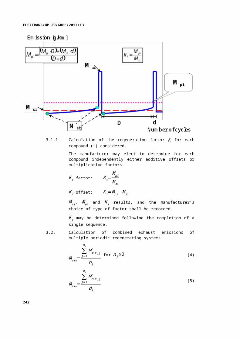
ECE/TRANS/WP.29/GRPE/2013/13
The end of charge criteria is reached when a fully charged REESS is detected by the on-board or external instruments.
242

ECE/TRANS/WP.29/GRPE/2013/13
Annex 8 - Appendix 5
Utility factor (UF) for OVC-HEVs
1. Utility Factor (UF) are ratios based on driver statistics and the ranges achieved in charge-depleting mode and charge-sustaining modes for OVC-HEVs and are used for weighting CO2 emissions and fuel consumptions.
2. Each Contracting Party may develop its own UFs.
243

ECE/TRANS/WP.29/GRPE/2013/13
[RESERVED: Annex 8, Appendix 6: Determining the range of PEVs on a per-phase basis]
244
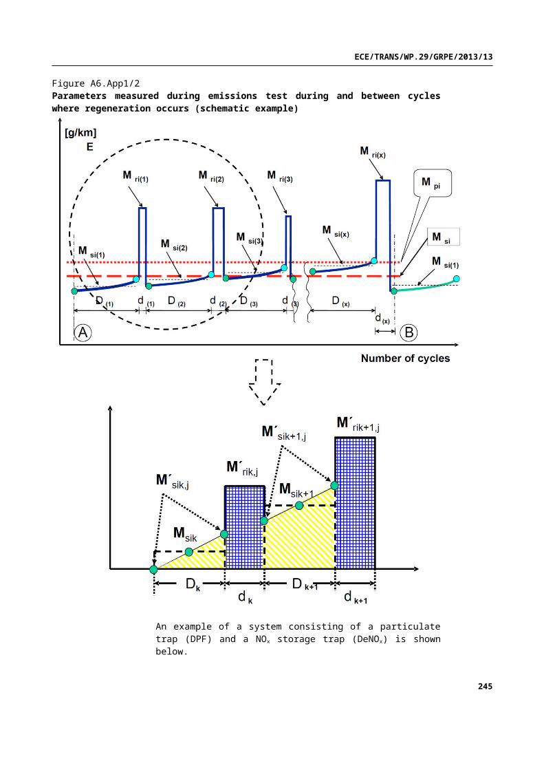
ECE/TRANS/WP.29/GRPE/2013/13
[Reserved: Annex 9 Determination of system equivalence]
245