United States Department of the Interior U. S. GEOLOGICAL SURVEY

Reston, VA 20192 In Reply Refer to: Mail Stops 412, 415

September 30, 2016 Office of Surface Water Technical Memorandum 2016.07 Office of Water Quality Technical Memorandum 2016.10

Subject: Policy and guidance for approval of surrogate regression models for computation of time series suspended-sediment concentrations and loads

BACKGROUND

The definition of a surrogate measure is a measurement taken with the intent to gain insight into a variable that is either impractical to measure directly, or not possible to measure at the desired continuous time interval. With a direct and uncomplicated causal relation, surrogate measurements can be nearly as useful as direct measurements although uncertainty associated with individual computed values generally is larger than discrete sample data. Increased temporal data richness could compensate for the larger uncertainty associated with computed data compared to laboratory results from actual samples.

In-situ turbidity, acoustic, and streamflow data, combined with discrete sample data, can be used to compute a time series of suspended-sediment concentrations and loads at stream sites. Two standard surrogate methods for computing time-series suspended sediment have been documented in U.S. Geological Survey (USGS) formal series Techniques and Methods reports. Rasmussen and others (2009) describe methods for developing regression models using in-situ turbidity and streamflow data, along with discrete samples of suspended-sediment concentrations. Landers and others (2016) describe sediment acoustic index methods for computing suspended-sediment concentrations. Both reports include detailed descriptions of methods for data collection, quality assurance and quality control, and data computation.

This technical memorandum describes reliable methods to develop statistical models specifically for suspended-sediment concentrations and loads based on surrogate measurements. The technical information herein does not apply to surrogate models for concentrations or loads of other water-quality constituents. This policy will facilitate a more consistent and streamlined approach for developing, documenting, and approving surrogate suspended-sediment regression models. Data computed as described in this memorandum meet USGS requirements for non-

2

interpretive information. Users can refer to the Office of Surface Water (OSW) Web site on Sediment for updated model examples, R scripts, and other tools as they become available.

PURPOSE

The purpose of this memorandum is to provide policy and guidance for developing and approving regression models used to compute high temporal frequency time series suspended-sediment concentrations and loads from continuous turbidity or acoustic backscatter data and continuous streamflow data that can be published without the need for documentation in a Bureau-approved interpretive report. As such, computed data from a statistical surrogate model must meet the definition of data rather than interpreted data. This policy applies to surrogate approaches in which continuous (measurement interval every hour or less) in-situ turbidity, acoustic, and/or streamflow data are used in combination with discrete suspended-sediment samples to develop regression models for computing similar continuous suspended-sediment concentration or load data.

POLICY

Computed suspended-sediment concentration and load data qualify as “non-interpretive” when the following conditions are met:

(1) Surrogate data and calibration samples are collected and laboratory analyses were performed using consistent sensor technologies (Rasmussen and others, 2009; Landers and others, 2016) and consistent USGS-approved and publicly available field methods for collection of suspended-sediment samples and continuous sensor data including U.S. Geological Survey (2006), Edwards and Glysson (1999), U.S. Geological Survey (2006), and Wagner and others (2006) and are analyzed for suspended-sediment concentration using USGS-approved laboratory methods, such as Guy (1969). Surrogate and calibration data used to develop the model must be available in the National Water Information System (NWIS) database. When guidance provided in this technical memorandum deviates from methods described in the previously-published methods reports, instructions in this memorandum should be followed.

(2) Computed data are derived from linear, log-linear, or log-log statistical models developed according to Ordinary Least Squares (OLS) regression methods described in published techniques and methods reports by Rasmussen and others (2009) and Landers and others (2016).

(3) Each model is documented in an electronic model archive summary (MAS) following guidance in this memorandum. The MAS meets model documentation requirements described in OSW Technical Memorandum (TM) 2015.01 and Office of Water Quality (OWQ) TM 2015.01, and is submitted for technical peer review, verification by the Water Science Field Team (WSFT) Specialist, and approval by the Center Director in lieu of the model archive contents

3

described in Attachment 2 of TM 2015.01. The MAS is stored in a reliable and publicly available location such as ScienceBase, the National Real-Time Water Quality (NRTWQ) Web site, or a future centralized Water Mission Area archive or repository.

The recommended steps for review and approval of the model and calibration dataset are: • The MAS, which includes the associated calibration dataset, is tracked in the Information

Product Data System (IPDS) as a single information product designated as a data release. • The MAS is reviewed by two technical peer reviewers at least one of whom is outside the

originating Center. • The reviewed MAS and Model Archive Verification and Approval Form (Attachment 1

of TM 2015.01) are submitted to the WSFT Specialist for verification that models have been adequately reviewed and archiving requirements are met, and the approval form is uploaded to IPDS.

• The MAS is assigned a Digital Object Identifier (DOI) and stored in a reliable and publicly available location.

• The MAS is approved by the Center Director following Fundamental Science Practices and Survey Manual (SM) SM 502.4 and SM 205.18.

(4) Once the MAS has been approved and publicly released, the computed suspended-sediment data may be disseminated to the public along with a link to the MAS in a USGS-approved database such as the NRTWQ Web site and NWIS using appropriate parameter codes as described in the Techniques and Methods reports (Rasmussen and others, 2009; Landers and others, 2016) without need for documentation in a Bureau-approved interpretive report.

(5) Continued sampling is required after model development to validate model performance if models are used to estimate suspended-sediment concentrations or loads on an on-going basis beyond the period of time that the model calibration samples were collected. Model validation is described in Attachment A of this memorandum and by Rasmussen and others (2009). Consistent with OWQ TM 2012.03, suspended-sediment samples must be submitted for laboratory analysis as soon as possible after collection and resulting data should be reviewed and approved promptly for use in model validation.

(6) Data interpolation defined as estimation between measured unit values and extrapolation defined as computation beyond the range of the model calibration dataset are permitted to a limited extent as described for acoustic methods by Landers and others (2016) and as otherwise described in Attachment A of this memorandum.

(7) Surrogate regression models as described in this memorandum are used to compute suspended-sediment concentration or load on the basis of observed explanatory variable(s) and cannot be used alone to predict future suspended-sediment concentration in the absence of a Bureau-approved interpretive report.

4

(8) Surrogate models and applications of this policy are reviewed during triennial technical reviews.

(9) This policy describes the standard approach for surrogate regression models for suspended sediment, and it must be followed when methods described by Rasmussen and others (2009) and Landers and others (2016) are used. Models documented in interpretive reports published previous to this memorandum may continue to be used if validation sampling and ongoing model evaluation (steps 4-8 in attachment A) are completed as described in this memorandum.

(10) A Bureau-approved interpretive report is required when conditions described in this memorandum are not met. This includes using alternative methods for collection of continuous and discrete data, sensor technologies, laboratory analyses, statistical model-building, and data computation. When alternative methods are used and documented in a separate report, a MAS similar to that described in this memorandum is required to document the model. If the model will be used for ongoing data computation, model validation and ongoing evaluation as described in items 4-8 of Attachment A is required unless circumstances warrant another approach. Robert R. Mason Donna N. Myers Chief, Office of Surface Water Chief, Office of Water Quality Distribution: All WMA Employees ATTACHMENTS

A. Policy and Guidance for Surrogate Suspended-Sediment Models

B. Example Model Archive Summary for a Turbidity Suspended-Sediment Model

C. Example Model Archive Summary for an Acoustic Suspended-Sediment Model

REFERENCES

Edwards, T.K., and Glysson, G.D., 1999, Field methods for measurement of fluvial sediment: U.S. Geological Survey Techniques of Water-Resources Investigations, book 3, chap. C2, 89 p., accessed March 7, 2016, at https://pubs.er.usgs.gov/publication/twri03C2.

Guy, H.P., 1969, Laboratory theory and methods for sediment analysis: U.S. Geological Survey Techniques of Water-Resources Investigations, book 5, chapter C1, 58 p.

Instructional Memorandum No. 2015.03, Review and approval of scientific data for release, accessed June 25, 2015 at http://www.usgs.gov/usgs-manual/im/IM-OSQI-2015-03.html

5

Landers, M.N., Straub, T.D., Wood, M.S., and Domanski, M.M., 2016, Sediment acoustic index method for computing continuous suspended-sediment concentrations: U.S. Geological Survey Techniques and Methods, book 3, chap. C5 at https://pubs.er.usgs.gov/publication/tm3C5

Office of Surface Water Technical Memorandum No. 2015.01, Policy and guidelines for archival of surface-water, groundwater, and water-quality model applications, accessed June 25, 2015 at http://water.usgs.gov/admin/memo/SW/sw2015.01.pdf

Office of Water Quality Technical Memorandum No. 2012.03, Update of policy on review and publication of discrete water data, accessed June 25, 2015 at http://water.usgs.gov/admin/memo/QW/qw12.03.pdf

Office of Water Quality Technical Memorandum No. 2015.01, Policy and guidelines for archival of surface-water, groundwater, and water-quality model applications, accessed June 25, 2015 at http://water.usgs.gov/admin/memo/QW/qw2015.01.pdf

Rasmussen, P.P., Gray, J.R., Glysson, G.D., and Ziegler, A.C., 2009, Guidelines and procedures for computing time-series suspended-sediment concentrations and loads from in-stream turbidity-sensor and streamflow data: U.S. Geological Survey Techniques and Methods book 3, chap. C4, 53 p, accessed June 25, 2016 at http://pubs.usgs.gov/tm/tm3c4/

Survey Manual 205.18, Authority to approve information products, accessed June 25, 2015 at http://www.usgs.gov/usgs-manual/200/205-18.html

Survey Manual 502.4, Fundamental Science Practices: Review, Approval, and Release of Information Products, accessed May 17, 2016 at http://www2.usgs.gov/usgs-manual/500/502-4.html

U.S. Geological Survey, 2006, Collection of water samples (ver. 2.0): U.S. Geological Survey Techniques of Water-Resources Investigations, book 9, chap. A4, September 2006, accessed June 25, 2016, at http://pubs.water.usgs.gov/twri9A4/.

Wagner, R.J., Boulger, R.W., Jr., Oblinger, C.J., and Smith, B.A., 2006, Guidelines and standard

procedures for continuous water-quality monitors—Station operation, record computation, and data reporting: U.S. Geological Survey Techniques and Methods 1-D3, 51 p. at https://pubs.usgs.gov/tm/2006/tm1D3/pdf/TM1D3.pdf

6

Attachment A. Requirements and Guidance for Surrogate Suspended-Sediment Models

The following information is provided to supplement methods described by Rasmussen and others (2009) and Landers and others (2016), and to provide additional policy implementation details. It includes a combination of requirements for meeting policy, emphasized using bold font, and guidance for best practices. In addition, the USGS National Training Center class “Environmental Statistics for Data Analysis,” QW1075, is recommended for data analysts. Experience or training in the R programming language is recommended. The Surrogate Analysis and Index Developer Tool (SAID) is available for developing surrogate models, particularly using acoustic methods, and SAID produces all of the information needed for the MAS (but not in the same MAS format). The MAS must follow the format described in this memorandum. An R script is available for this purpose at http://water.usgs.gov/osw/techniques/sediment.html, or the MAS can be prepared using tools of the user’s choice. Additional information may be appended at the end of the MAS if needed.

1. The model development process is documented in a model archive summary (MAS) that includes a written summary of the decisions made during the model-development process, the model form, several diagnostic statistics and graphs that indicate adequate model fit, predictive ability and uncertainty, list and explanation of outliers and how they were handled in model development, and a link to the complete model calibration data set. An example MAS for turbidity and streamflow regression models is provided in Attachment B. An example MAS for acoustic methods is provided in Attachment C.

2. A statistically valid number of samples are needed to develop, validate, and verify surrogate regression models over time. Samples must be collected over a range of conditions. In the model archive summary, the modeler must provide specific, detailed justification as to why the number of samples used for surrogate model development is sufficient to represent the population of data for which predictions are being made. Such justification must include the sufficiency of the data to describe seasonal, hydrologic, particle size, or any other factors that could possibly affect the surrogate relation.

• Model builders need to be cognizant of the possibility of overfitting their surrogate model.

Overfitted models adhere too closely to the idiosyncrasies of a particular data set that do not actually appear in the population of data being modeled (Babyak, 2004). One way to guard against overfitting is to have an adequate number of sample observations per each explanatory variable in the model. A long used rule of thumb is 10-15 observations per explanatory variable (Babyak, 2004). Harrell (2001, pg. 61) recommends 10-20 observations per explanatory variable. So for a simple linear regression model, 20-40 observations are necessary (10-20 for both the intercept and the single explanatory variable). Green (1991) recommended 50 observations plus 8 additional observations for each explanatory variable. The number of samples also needs to sufficiently represent all

7

seasonal, hydrologic, and other conditions potentially affecting the model, and to allow for evaluating the predictive performance of the model. Model fit statistics, such as coefficient of determination (R2) and mean square error, are not necessarily good measures of how well a model will predict outside the calibration data set. Cross-validation is a good method for measuring this. For example, the cross-validation information in Attachment B indicates that when the model calibration data are randomly divided into subsets, the predictions from each subset regression model are very similar to the final surrogate model. Thus, for surrogate suspended-sediment models, a recommended minimum of 36 suspended-sediment samples is generally considered adequate for developing and validating a model with one explanatory variable, for example, turbidity. This number is based on the mid-range of sample sizes recommended in the literature with an additional 20 percent increase to allow for an adequate cross-validation analysis to assess predictive capability of the model. An additional 12 samples, for a minimum of 48 samples, is recommended for a model with two explanatory variables, for example turbidity and streamflow.

• Samples must be representative of the stream cross-section and can be equal width increment (EWI) samples, equal discharge increment (EDI) samples, or fixed-point pump samples that have been adjusted using concurrent cross-section samples (Landers and others, 2016, p. 13; Edwards and Glysson, 1999, p. 31). The relation of fixed-point to EWI/EDI samples must be documented in the analysis and model archive summary. Samples also must be statistically independent within reason and should be tested for autocorrelation following methods described by Landers and others (2016). If the independence assumption is not met, then appropriate non-OLS statistical methods must be used to fit the model and it must be documented in a separate Bureau-approved interpretive report (Rasmussen and others, 2009, p. 11; Landers and others, 2016, p. 30). Particle-size analysis for samples is not required, but sand/silt split data often are very helpful when evaluating dataset variability and outliers (Rasmussen and others, 2009).

• The sampling design must ensure that samples are representative of the system being modeled. It is recommended that about half of the samples are collected at fixed intervals (monthly), and half of the samples are collected during runoff events or targeting other sources of variability.

• The recommended period to collect data for model development is 3 years, but generally should range from 2-6 years. If data are collected over just 1 year for model development, additional validation samples are needed in subsequent years if hydrologic conditions are different. Data collected over more than 6 years should be tested for violation of stationarity assumptions and appropriate actions taken to address it.

8

3. The data analyst submits the MAS to two qualified technical peer reviewers. Qualified technical reviewers are those with scientific and technical expertise relevant to sound regression model development. The reviewers evaluate the model and recommend the MAS be either approved or rejected. If a model is rejected, the data analyst has the option to redevelop the model and MAS based on the reviewer’s suggestions, and then submit it for additional technical review. Before the surrogate regression model is used to compute data to be delivered to the public, the Center Director must approve the MAS as described in the Policy section of this technical memorandum.

4. Data to validate model performance are required for any model used to estimate constituent values outside of the period of data collection used for model calibration. Validation data must be available in the National Water Information System (NWIS) (http://dx.doi.org/10.5066/F7P55KJN). • A minimum of 8 validation samples per year on average are required to be collected with

a minimum of 6 in any given year. This is a larger number than recommended by Rasmussen and others (2009) and Landers and others (2016) to better assess departures from the model and allow sufficient data to refit models if needed. Validation samples are flow-weighted composite samples collected from the channel cross-section (EWI/EDI when possible) using approved field protocols (USGS, 2006; Edward and Glysson, 1999) or fixed-point pump samples as previously described. Four of these samples are to be collected at a quarterly interval, that is, the samples are to be collected about 3 months apart and four samples are to be targeted toward time periods of variability in the system. Exceptions to this guidance may exist, including:

a. For many situations, variations in streamflow present the greatest source of variability and these four additional samples should be targeted to capture high flows that are often characterized by high suspended-sediment concentrations, and should include rising, peak, and falling limbs of the hydrograph.

b. Targeted samples should be spread throughout the year unless the variability is limited to shorter periods in which case the targeted samples should be spread throughout the period of variability. For example, for streams affected by storms throughout the year, the samples targeting storm runoff would be spread throughout the year. However, for streams where flow is affected mainly by snowmelt or pronounced wet and dry (or ephemeral) periods, the targeted samples may be spread only throughout the snowmelt or the wet and dry periods.

• Because validation samples are collected at least quarterly, models can be used for data estimation no longer than about 3 months after the last validation sample has been collected.

5. As soon as practicable after each validation sample is collected, performance of the model with respect to that sample should be assessed. The residual from the predicted value

9

associated with a validation sample should be assessed in the same manner as a residual from the model calibration data set.

• The recommended approach for ongoing model validation is conceptually based on the runs test for randomness in residuals (Hipel and McLeod, 1994, p. 942). A run is a consecutive sequence of positive or negative residuals. The runs test estimates the probability of the number of runs observed happening solely due to chance. For surrogate models, there will be insufficient data available to compute a formal runs test for several years (based on the recommended number of validation samples collected per year). Thus an approach based on consecutive large positive or negative residuals computed from the predicted values and observed concentrations from the validation samples should be used instead. The consecutive occurrence of even a few large residuals with the same sign has a very low probability of occurring due to chance. The presence of one or more of these large residuals is an early warning of possible considerable bias in the values predicted by the surrogate model that warrants investigation.

a. If the residual from one validation sample has a value of about 2 to 3 standard errors from the predicted value, the operation of sensors and equipment providing input to the surrogate model should be checked to make sure nothing is malfunctioning. Anomalies in the watershed should also be investigated. The probability of a residual falling within this range from a well-fit model is about 0.01 to 0.05.

b. If there are two consecutive validation samples that have a residual value of about 2 to 3 standard errors from the predicted value with both having the same sign either positive or negative, check equipment again for malfunctions and check for anomalies in the watershed. If all equipment is operating correctly and no anomalies are found, then collect an additional validation sample at the next site visit or within 30 days, if possible during conditions similar to those when samples with large residuals were collected. The probability of two independent consecutive residuals falling within the range of 2 to 3 standard errors from the predicted value from a well-fit model is about 0.0001 to 0.0025.

c. If there is a third consecutive validation sample that has a residual value of 2 to 3 standard errors from the predicted value (with all three having the same sign, that is all three residuals being either positive or negative), then the model must be assumed to be flawed and must be refit using all data collected since the release of the previous model including the 3 recent validation samples with large residuals. The probability of three independent consecutive residuals falling within the range of 2 to 3 standard errors from the predicted value from a well-fit model is about 0.000001 to 0.000125.

10

d. If the residual has a value greater than 3 standard errors from the predicted value and sensors and equipment are not malfunctioning and no watershed anomalies are found, then collect an additional validation sample at the next site visit or within 30 days. The probability of a residual being greater than 3 standard errors from the predicted value from a well-fit model is less than about 0.01.

e. If there are two consecutive validation samples that have a residual value greater than 3 standard errors from the predicted value, regardless of the sign of the residual, then the model must be assumed to be flawed and must be refit using all data collected since the release of the previous model including the 2 recent validation samples with large residuals. The probability of two independent consecutive residuals both being greater than 3 standard errors from the predicted value from a well-fit model is less than about 0.0001.

• If the refit model is deemed adequate by following the same process used to fit the original model, the refit model will replace the existing model and predicted values from the first validation sample whose residual exceeds the 2 standard error threshold will be re-estimated using the refit model. A new model archive package must be prepared and approved following the same process as the original model prior to use of the refit model.

• If the refit model is deemed inadequate, use of the model must be discontinued completely or until additional sample data are collected and an adequate model can be developed by making adjustments that are consistent with the Techniques and Methods reports. For example, the original model might use turbidity as a single explanatory variable, and the refit model might use both turbidity and streamflow as explanatory variables, which is consistent with the Techniques and Methods report.

6. Surrogate sediment models must be reviewed annually, typically after the continuous data

used as a surrogate have been approved and the discrete sample results used in the model have been reviewed and approved. This review occurs even when no validation samples exceed the large residual thresholds discussed in the previous section of this guidance. The annual review should include all of the following: • Review plots of all validation sample residuals collected during the year against time,

predicted values, and explanatory variables. Compare residuals from samples collected during the current year to those collected in previous years. Look for patterns in the current year residuals that might indicate a change or shift in the relation between the response and explanatory variables used in the model.

11

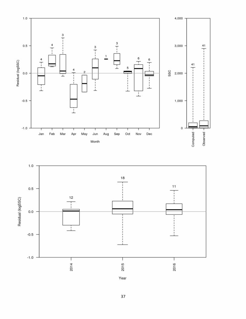
• Review a boxplot of the validation sample residuals by year. Compare the distribution of residuals from samples collected during the current year to those collected in previous years.

• Review a boxplot of validation sample residuals by seasonal periods. Note this can only be done after several years of additional data collection if just the minimum eight validation samples per year are being collected. Also, fewer than the four seasons per year can be used if necessary to obtain enough data to create boxplots. An example of this might be looking at boxplots for three 4-month periods rather than four 3-month periods. Look for seasonal patterns in the residuals that might indicate a temporal change or shift in the relation between the response and explanatory variables used in the model.

• A narrative describing the annual model review must be written describing why the modeler believes there is no problem with the existing surrogate model or if a problem is identified how it was addressed. This narrative is analogous to the annual gaging station analysis that is prepared for each streamgage. Annual model review is documented in the Records Management System (RMS).

• Best practice usually is to start a new model within 6 months of the data collection period. When a revised model is developed, best practice is usually to start applying the model when it is approved; however, users may choose to apply the model beginning at the time that samples indicated deviation from the previous model.

7. Even if no problems are identified during the annual model review, surrogate models must

still be refit every 3 years with the additional validation samples collected during the ongoing 3-year period and documented in a new MAS. Routine model updates take advantage of additional collected data to ensure models are current and reduce model uncertainty and likelihood of stationarity issues. • The initial refitting of the model should use the same form as the model being updated.

However, the adequacy of the model form should be examined and if necessary alternative forms of the model should be explored.

• The data analyst will need to pay particular attention to the residual versus time plots for the refit model. If residuals early in the time series show patterns or otherwise depart from random noise about the zero reference line, it is an indication of a shift in the underlying processes driving the model. Sample observations from the earlier period of the sample time series should then be removed from the calibration dataset, removing as few as possible to address the lack of fit in the early periods of the model to see if an adequate model may be obtained. However, if removing sample observations reduces the minimum

12

number of samples for model building below the minimum number recommended or to a time span of less than 2 years, additional data will be needed until those criteria are again met. Decisions and reasoning related to sample time series used in model development must be documented in the MAS.

• A new model archive summary package is to be prepared and approved following the same process described for the original model including approval in IPDS before the updated model is used.

• Centers must use good judgment in deciding when a new model becomes effective. The general recommendation is that the model becomes effective as soon after approval as practical.

8. Extrapolation for acoustic models is allowed as described by Landers and others (2016).

Limited extrapolation is allowed as described below for approved models developed following methods described by Rasmussen and others (2009). • Approved models developed following Rasmussen and others (2009) may be used to

extrapolate no more than 10 percent (calculated using retransformed units rather than log units) outside of the range of the sample data used to fit the model with no additional sample collection required. For models following Rasmussen and others (2009), extrapolation must not exceed the manufacturer’s specifications for the optimal performance range of the turbidity sensor. Approved models following Landers and others (2016) may be used to extrapolate no more than 20 percent outside the range of sample data used to fit the model.

• Approved models may be used to extrapolate more than 10 percent following Rasmussen and others (2009) and more than 20 percent following Landers and others (2016) if an additional validation sample in that extrapolated range can be collected during the same season and within about 90 days provided that channel conditions have not changed for either method.

a. If the validation sample confirms that model predictions are accurate in the extrapolation range with validation data then predicted values may be kept and accepted as final data for display in NWISWeb or NRTWQ

b. If the validation sample does not confirm that model predictions are accurate in the extrapolation range, then predicted values must either be: o censored at greater than the predicted value if the validation sample confirms

that the direction of the model bias is indeed positive; for example, the model prediction is 100 but the validation sample is 200 then the predicted values may be set to >100, or

13

o removed or blocked in NWIS using thresholds if the validation sample does not confirm the direction of the model bias; for example, the model prediction is 100 but validation sample is 50.

• Approved models may not be used for extrapolating more than 20 percent outside the range of the sample data used to fit the model until additional data are collected in that range and the model performance and sensor performance are validated or the model is refit using the new data. A minimum of one (but at least two are recommended) independent samples must be collected outside the range of the existing data to confirm the model is performing adequately. Model predictions made outside of the two previously mentioned allowable areas of extrapolation may not be served in the real-time water quality system and they must be removed or blocked in NWIS until the existing model is validated with the new data or a new model is fit that includes data in the range. Once a new model is approved, it may be used to make predictions for any data previously blocked in NWIS.

• Approved models shall not be used for interpolating between time intervals for which the surrogate data are collected. That is, if surrogate data are collected at 30-minute intervals, the models may not be used to estimate at 15-minute intervals by averaging or otherwise interpolating between values of the surrogates collected at the longer time step.

9. Approved models can be disseminated and archived on the NRTWQ Web site

(http://nrtwq.usgs.gov/). These time series are displayed in plots, tables, statistical summaries, and duration curves. Site and model information are also displayed. These computed values also can be displayed using NWIS, or using another approved data release method. As new models are employed, older models are archived along with the computed data. Models are numbered sequentially and include the station number, constituent, year the model was approved, and model version number if needed (for example, 06892350.SSC.WY15.ver1).

10. Surrogate turbidity and streamflow data for computed concentrations and loads are considered category 1 data and are approved by following the Continuous Records Processing (CRP) policy of the Water Mission Area (WRD Policy Numbered Memorandum 2010.02). Methods of collecting the surrogate measurements are documented in formal publications series such as USGS Techniques and Methods or the National Field Manual. Computed concentration and loads are approved following CRP policy under category 3 which indicates approval to be completed within a year in most cases. All surrogate data must be stored in NWIS.

11. Circumstances may arise in which historical data need revision. For example, if errors are discovered in explanatory data such as turbidity, then errors also exist in computed

14

suspended sediment data. Until further guidance is provided, Centers must use good judgment in deciding which circumstances justify correction of historical data.

References

Babyak, M.A., 2004, What you see may not be what you get-A brief, nontechnical introduction to overfitting in regression-type models: Psychosomatic Medicine, v. 66, no. 3, p. 411-421.

Edwards, T.K., and Glysson, G.D., 1999, Field methods for measurement of fluvial sediment: U.S. Geological Survey Techniques of Water-Resources Investigations, book 3, chap. C2, 89 p., accessed March 7, 2016, at https://pubs.er.usgs.gov/publication/twri03C2.

Green, S.B., 1991, How many subjects does it take to do a regression analysis: Multivariate Behavioral Research, v. 26, no. 3, p.499-510.

Harrell, F.E., Jr., 2001, Regression Modeling Strategies-With Applications to Linear Models, Logistic Regression, and Survival Analysis: Springer, New York, 568 p.

Hipel, K.W., and McLeod, A.I., 1994, Modelling of Water Resources and Environmental Systems: Amsterdam, Elsevier, 1013 p.

Landers, M.N., Straub, T.D., Wood, M.S., and Domanski, M.M., 2016, Sediment acoustic index method for computing continuous suspended-sediment concentrations: U.S. Geological Survey Techniques and Methods, book 3, chap. C5

Rasmussen, P.P., Gray, J.R., Glysson, G.D., and Ziegler, A.C., 2009, Guidelines and procedures for computing time-series suspended-sediment concentrations and loads from in-stream turbidity-sensor and streamflow data: U.S. Geological Survey Techniques and Methods book 3, chap. C4, 53 p.

U.S. Geological Survey, 2006, Collection of water samples (ver. 2.0): U.S. Geological Survey Techniques of Water-Resources Investigations, book 9, chap. A4, September 2006, accessed June 25, 2016, at http://pubs.water.usgs.gov/twri9A4/

WRD Policy Numbered Memorandum No. 2010.02, Continuous Records Processing of all Water Time Series Data, accessed July, 2016 at http://water.usgs.gov/admin/memo/policy/wrdpolicy10.02.html

15

Attachment B. Example Model Archive Summary for a Turbidity Suspended-Sediment Model

Model Archive Summary for Suspended-Sediment Concentration at Station 07144100; Little Arkansas River near Sedgwick, Kansas This model archive summary summarizes the suspended-sediment concentration (SSC) model developed to compute hourly SSC from January 1, 2007 onward. This model supersedes all models used from 2007 onward. The methods used follow USGS guidance as referenced in relevant Office of Surface Water/Office of Water Quality Technical Memoranda and USGS Techniques and Methods, book 3, chap. C4 (Rasmussen and others, 2009).

Site and Model Information

Site number: 07144100

Site name: Little Arkansas River near Sedgwick, Kansas

Location: Latitude 37°52'59", longitude 97°25'27" referenced to North American Datum of 1927, in NE ¼ NW ¼ NW ¼ sec. 15, T. 25 S., R. 1 W., Sedgwick County, Kansas, Hydrologic Unit 11030012, on left bank at downstream side from county highway bridge, 2.1 miles (mi) south of Sedgwick, and at mile marker 23.7.

Equipment: A YSI 6600 water-quality monitor equipped with sensors for water temperature, specific conductance (SC), dissolved oxygen, and pH, and a YSI Model 6136 turbidity sensor. The monitor is housed in a 4-inch plastic pipe and typically is placed in the deepest section of the river that has velocity similar to rest of the stream. Readings from the YSI 6600 are recorded every 30 minutes and transmitted by way of satellite, hourly. A YSI Model 6136 turbidity sensor started operation July 27, 2004.

Model number: 07144100.SSC.WY07.1

Date model was created: December 26, 2014

Model calibration data period: July, 27 2004 to August 4, 2014

Model application date: January 1, 2007 onward

Computed by: Patrick Eslick, KS WSC, June 21, 2016

Reviewed by: Patrick Rasmussen, KS WSC and Brian Kelly, KS WSC, July 8, 2016

Approved by: Andy Ziegler, KS WSC Director, July 20, 2016

Model Data All data were collected using U.S. Geological Survey (USGS) protocols and are stored in the National Water Information System (NWIS) database (http://dx.doi.org/10.5066/F7P55KJN). The regression model is based on 120 concurrent measurements of suspended-sediment concentration, streamflow, and turbidity samples collected from July 27, 2004 through August 4, 2014. Samples were collected throughout the range of continuously observed hydrologic and turbidity conditions. Summary statistics and the complete model-calibration data are provided in the dataset. Studentized residuals from the final model were inspected for values greater than 3 or less than negative 3. Values outside of the 3 to -3 range are considered potential outliers and were investigated. Samples collected May 29, 2008; December 1, 2009; December 17, 2009; and December 11, 2013; June 13, 2010; July 6, 2010; and August 15, 2013 were deemed outliers and were removed from the dataset.

16

Sediment Data Cross-section samples are collected either from the downstream side of the bridge or instream upstream near the bridge. The equal-width-increment or multi-vertical method is used, and samples typically are composited for analysis. Cross-section samples are obtained during all discrete sample collections every month and during selected runoff events. A FISP US D-95 with a Teflon bottle, cap, and nozzle depth-integrating sampler is used from the bridge; and a DH-81with a Teflon bottle, cap, and nozzle hand sampler or a grab sample with a Teflon bottle is used for wading samples. Samples are analyzed for SSC and/ or LOI and 5-point grain size in the USGS Sediment Laboratory in Iowa City, Iowa.

Surrogate Data The turbidity data used in this analysis were measured using a YSI model 6136 installed and in use from 2007 onward. The 6136 replaced the old YSI model 6026 sensor. Data from the YSI 6026 and 6136 sensors are not equivalent and therefore cannot be used interchangeably with this new SSC model. See the Station Analysis for the streamflow and turbidity records for more information (available upon request).

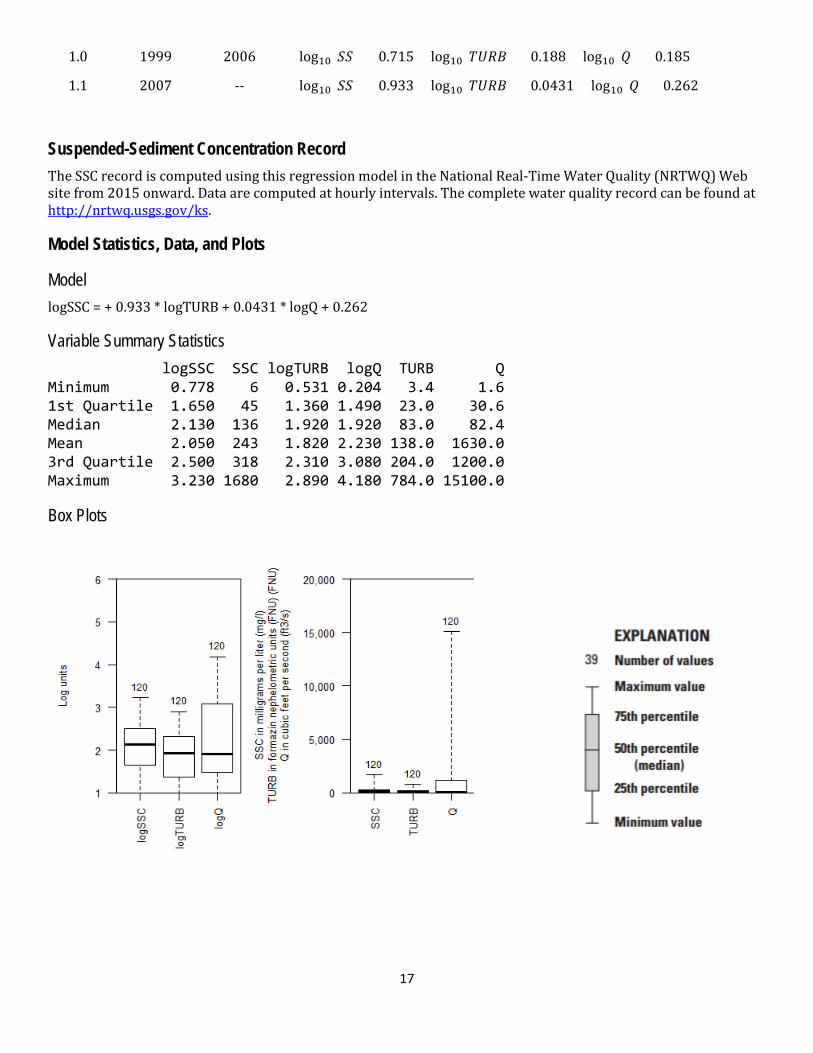
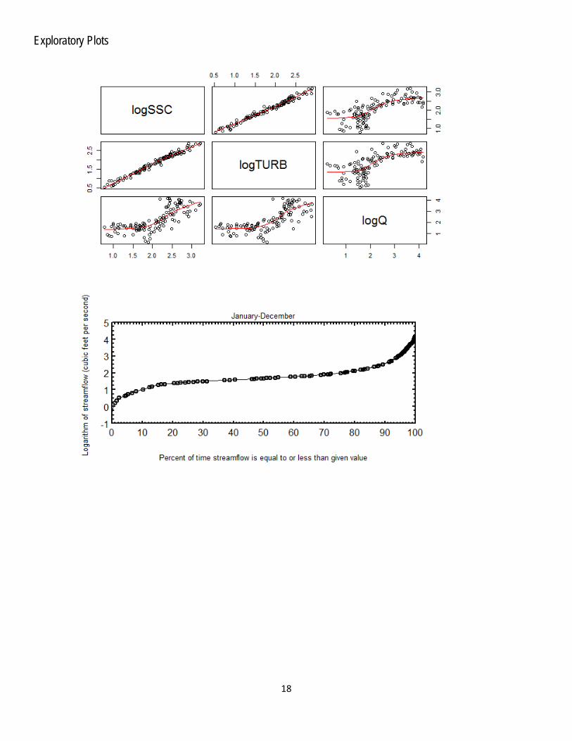
Model Development Regression analysis was done using R by examining turbidity and other continuously measured data as explanatory variables for estimating suspended-sediment concentration. A variety of models that predict SSC and models that predict log10(SSC) were evaluated. The distribution of residuals was examined for normality and plots of residuals (the difference between the measured and predicted values) as compared to predicted SSC were examined for homoscedasticity (meaning that their departures from zero did not change substantially over the range of predicted values). This comparison of several models led to the conclusion that the most appropriate and reliable model would be one that estimated log10(SSC). Turbidity and streamflow were selected as the best predictors of log10(SSC) based on residual plots, relatively high adjusted coefficient of determination (adjusted R2), and relatively low model standard percentage error (MSPE). Values for all of the aforementioned statistics and metrics were computed and are included below along with all relevant sample data and more in-depth statistical information.

Model Summary Summary of final regression analysis for suspended-sediment concentration at site number 07144100. Suspended-sediment concentration-based model: log10(𝑆𝑆𝑆) = 0.933 × log10(𝑇𝑇𝑇𝑇) + 0.0431 × log10(𝑄) + 0.262 , where SSC = suspended-sediment concentration, in milligrams per liter (mg/L); Q = streamflow in cubic feet per second (ft3/s); and, TURB = Turbidity, YSI model 6136, in formazin nephelometric units (FNU). The use of turbidity and streamflow as explanatory variables is appropriate physically and statistically. Turbidity makes sense physically because suspended sediment is composed of particles that scatter light in water. Suspended sediment correlates well with streamflow because high streamflow values tend to increase concentrations of SSC. The relation between turbidity and SSC can vary given varying concentrations of organic suspended particles that increase turbidity, but are not included in the SSC analysis. The log-transformed model may be retransformed to the original units so that SSC can be calculated directly. The retransformation introduces a bias in the calculated constituent. This bias may be corrected using Duan’s Bias Correction Factor (BCF). For this model, the calculated BCF is 1.02. The retransformed model, accounting for BCF is:

𝑆𝑆 = 1.865 × 𝑇𝑇𝑇𝑇0.933 × 𝑄0.0431.

Previous models Model Start year End year Model

17

1.0 1999 2006 log10(𝑆𝑆) = 0.715 × log10(𝑇𝑇𝑇𝑇) + 0.188 × log10(𝑄) + 0.185

1.1 2007 -- log10(𝑆𝑆) = 0.933 × log10(𝑇𝑇𝑇𝑇) + 0.0431 × log10(𝑄) + 0.262

Suspended-Sediment Concentration Record The SSC record is computed using this regression model in the National Real-Time Water Quality (NRTWQ) Web site from 2015 onward. Data are computed at hourly intervals. The complete water quality record can be found at http://nrtwq.usgs.gov/ks.

Model Statistics, Data, and Plots

Model logSSC = + 0.933 * logTURB + 0.0431 * logQ + 0.262

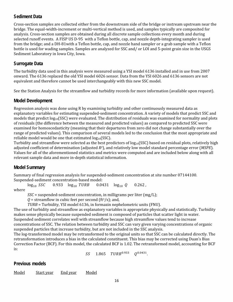
Variable Summary Statistics logSSC SSC logTURB logQ TURB Q Minimum 0.778 6 0.531 0.204 3.4 1.6 1st Quartile 1.650 45 1.360 1.490 23.0 30.6 Median 2.130 136 1.920 1.920 83.0 82.4 Mean 2.050 243 1.820 2.230 138.0 1630.0 3rd Quartile 2.500 318 2.310 3.080 204.0 1200.0 Maximum 3.230 1680 2.890 4.180 784.0 15100.0

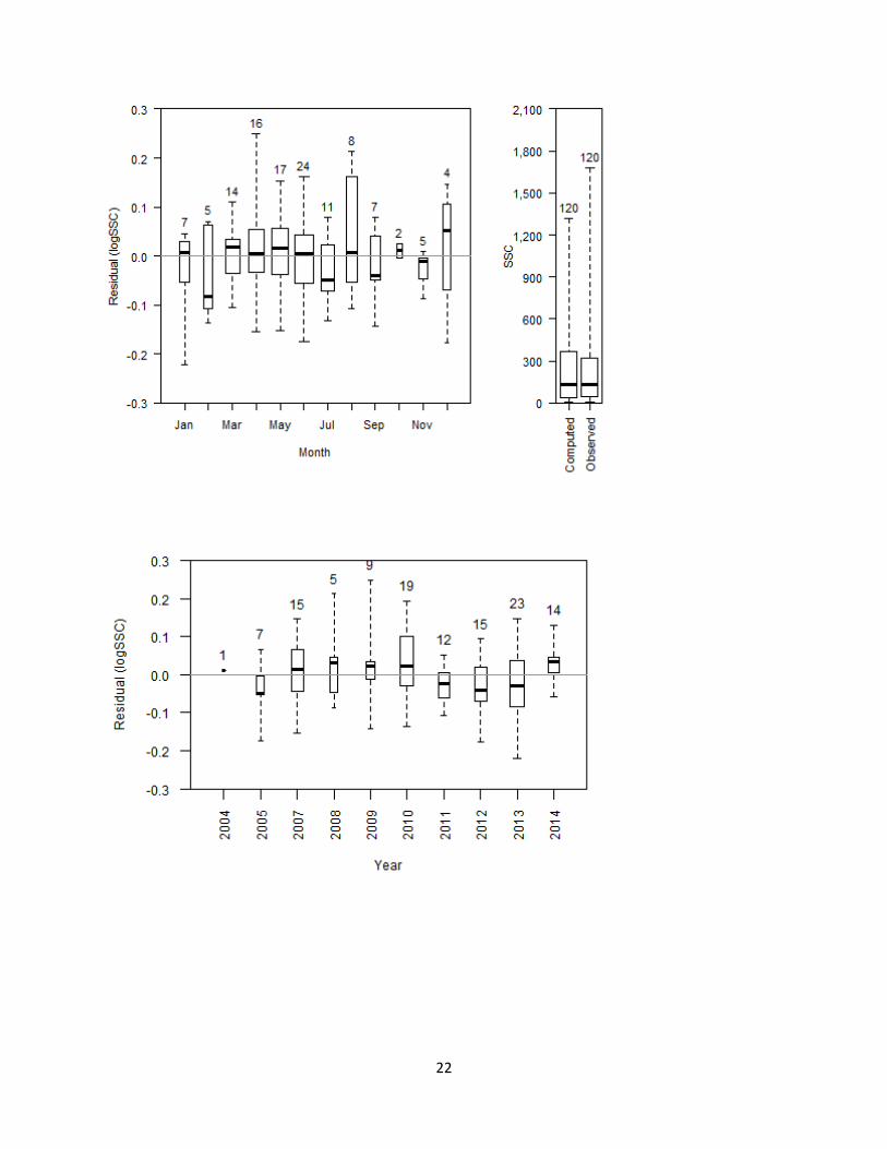
Box Plots

18

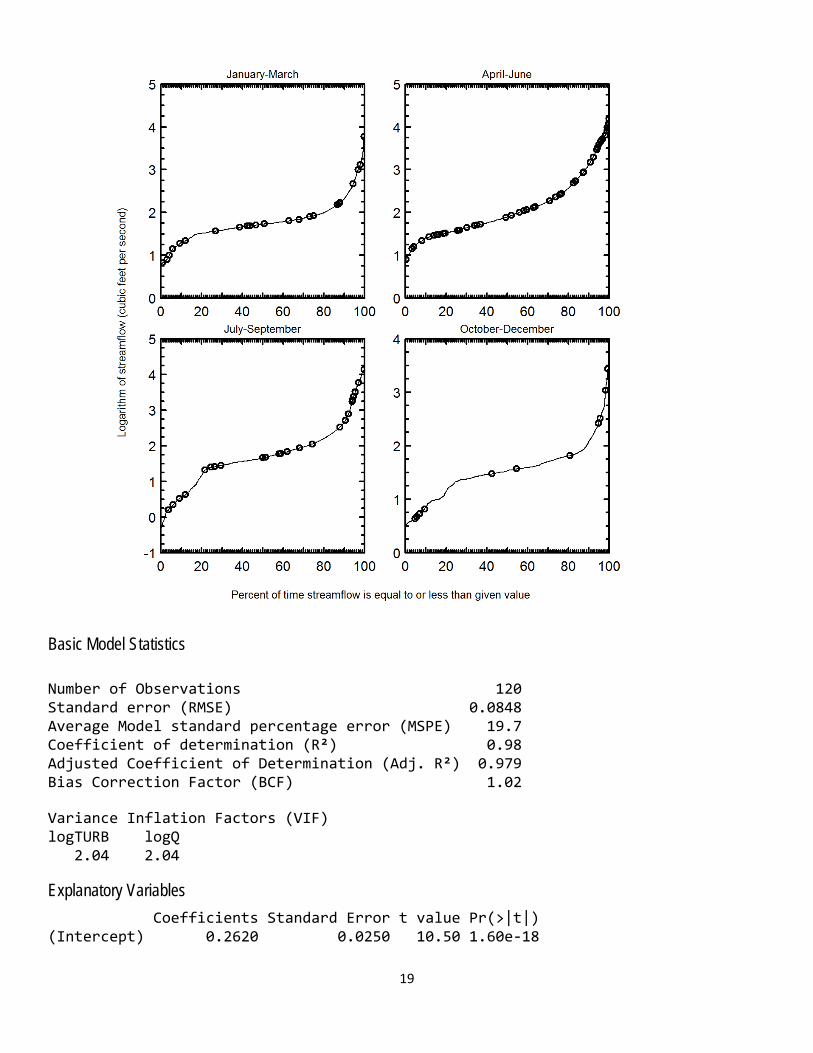
Exploratory Plots

19

Basic Model Statistics Number of Observations 120 Standard error (RMSE) 0.0848 Average Model standard percentage error (MSPE) 19.7 Coefficient of determination (R²) 0.98 Adjusted Coefficient of Determination (Adj. R²) 0.979 Bias Correction Factor (BCF) 1.02 Variance Inflation Factors (VIF) logTURB logQ 2.04 2.04

Explanatory Variables Coefficients Standard Error t value Pr(>|t|) (Intercept) 0.2620 0.0250 10.50 1.60e-18

20

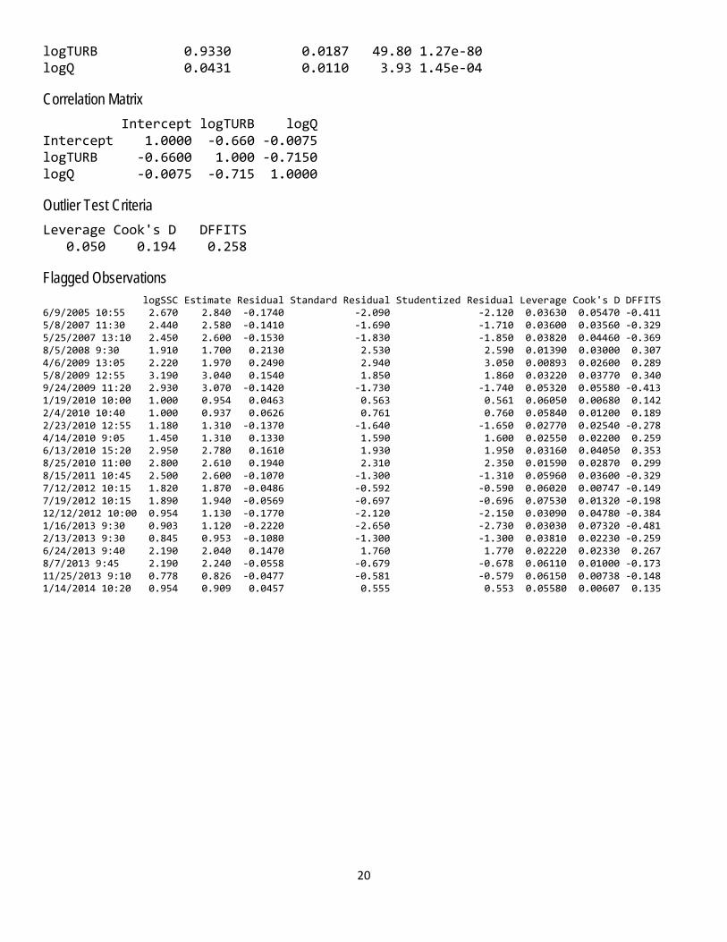
logTURB 0.9330 0.0187 49.80 1.27e-80 logQ 0.0431 0.0110 3.93 1.45e-04

Correlation Matrix Intercept logTURB logQ Intercept 1.0000 -0.660 -0.0075 logTURB -0.6600 1.000 -0.7150 logQ -0.0075 -0.715 1.0000

Outlier Test Criteria Leverage Cook's D DFFITS 0.050 0.194 0.258

Flagged Observations logSSC Estimate Residual Standard Residual Studentized Residual Leverage Cook's D DFFITS 6/9/2005 10:55 2.670 2.840 -0.1740 -2.090 -2.120 0.03630 0.05470 -0.411 5/8/2007 11:30 2.440 2.580 -0.1410 -1.690 -1.710 0.03600 0.03560 -0.329 5/25/2007 13:10 2.450 2.600 -0.1530 -1.830 -1.850 0.03820 0.04460 -0.369 8/5/2008 9:30 1.910 1.700 0.2130 2.530 2.590 0.01390 0.03000 0.307 4/6/2009 13:05 2.220 1.970 0.2490 2.940 3.050 0.00893 0.02600 0.289 5/8/2009 12:55 3.190 3.040 0.1540 1.850 1.860 0.03220 0.03770 0.340 9/24/2009 11:20 2.930 3.070 -0.1420 -1.730 -1.740 0.05320 0.05580 -0.413 1/19/2010 10:00 1.000 0.954 0.0463 0.563 0.561 0.06050 0.00680 0.142 2/4/2010 10:40 1.000 0.937 0.0626 0.761 0.760 0.05840 0.01200 0.189 2/23/2010 12:55 1.180 1.310 -0.1370 -1.640 -1.650 0.02770 0.02540 -0.278 4/14/2010 9:05 1.450 1.310 0.1330 1.590 1.600 0.02550 0.02200 0.259 6/13/2010 15:20 2.950 2.780 0.1610 1.930 1.950 0.03160 0.04050 0.353 8/25/2010 11:00 2.800 2.610 0.1940 2.310 2.350 0.01590 0.02870 0.299 8/15/2011 10:45 2.500 2.600 -0.1070 -1.300 -1.310 0.05960 0.03600 -0.329 7/12/2012 10:15 1.820 1.870 -0.0486 -0.592 -0.590 0.06020 0.00747 -0.149 7/19/2012 10:15 1.890 1.940 -0.0569 -0.697 -0.696 0.07530 0.01320 -0.198 12/12/2012 10:00 0.954 1.130 -0.1770 -2.120 -2.150 0.03090 0.04780 -0.384 1/16/2013 9:30 0.903 1.120 -0.2220 -2.650 -2.730 0.03030 0.07320 -0.481 2/13/2013 9:30 0.845 0.953 -0.1080 -1.300 -1.300 0.03810 0.02230 -0.259 6/24/2013 9:40 2.190 2.040 0.1470 1.760 1.770 0.02220 0.02330 0.267 8/7/2013 9:45 2.190 2.240 -0.0558 -0.679 -0.678 0.06110 0.01000 -0.173 11/25/2013 9:10 0.778 0.826 -0.0477 -0.581 -0.579 0.06150 0.00738 -0.148 1/14/2014 10:20 0.954 0.909 0.0457 0.555 0.553 0.05580 0.00607 0.135

21

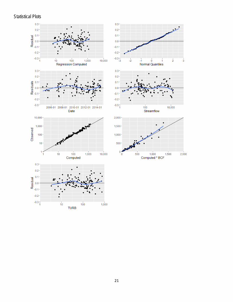
Statistical Plots

22

23

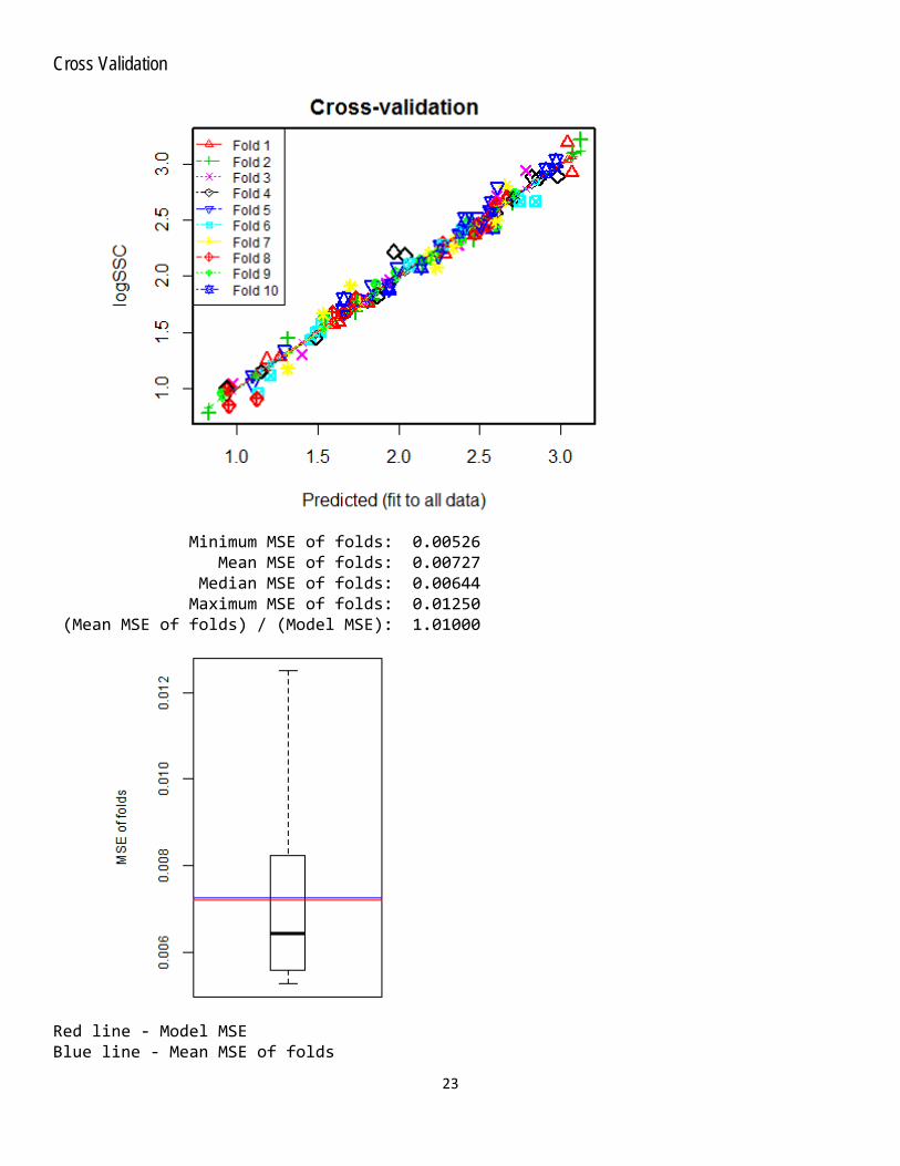
Cross Validation

Minimum MSE of folds: 0.00526 Mean MSE of folds: 0.00727 Median MSE of folds: 0.00644 Maximum MSE of folds: 0.01250 (Mean MSE of folds) / (Model MSE): 1.01000

Red line - Model MSE Blue line - Mean MSE of folds

24

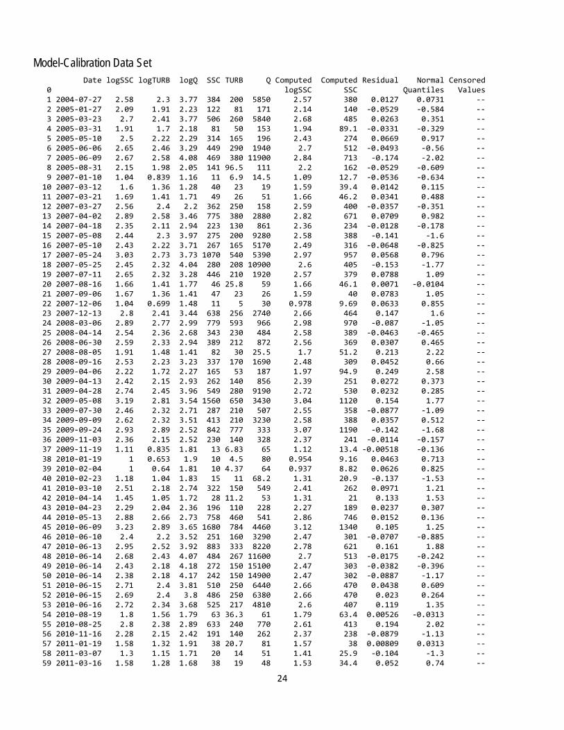
Model-Calibration Data Set Date logSSC logTURB logQ SSC TURB Q Computed Computed Residual Normal Censored 0 logSSC SSC Quantiles Values 1 2004-07-27 2.58 2.3 3.77 384 200 5850 2.57 380 0.0127 0.0731 -- 2 2005-01-27 2.09 1.91 2.23 122 81 171 2.14 140 -0.0529 -0.584 -- 3 2005-03-23 2.7 2.41 3.77 506 260 5840 2.68 485 0.0263 0.351 -- 4 2005-03-31 1.91 1.7 2.18 81 50 153 1.94 89.1 -0.0331 -0.329 -- 5 2005-05-10 2.5 2.22 2.29 314 165 196 2.43 274 0.0669 0.917 -- 6 2005-06-06 2.65 2.46 3.29 449 290 1940 2.7 512 -0.0493 -0.56 -- 7 2005-06-09 2.67 2.58 4.08 469 380 11900 2.84 713 -0.174 -2.02 -- 8 2005-08-31 2.15 1.98 2.05 141 96.5 111 2.2 162 -0.0529 -0.609 -- 9 2007-01-10 1.04 0.839 1.16 11 6.9 14.5 1.09 12.7 -0.0536 -0.634 -- 10 2007-03-12 1.6 1.36 1.28 40 23 19 1.59 39.4 0.0142 0.115 -- 11 2007-03-21 1.69 1.41 1.71 49 26 51 1.66 46.2 0.0341 0.488 -- 12 2007-03-27 2.56 2.4 2.2 362 250 158 2.59 400 -0.0357 -0.351 -- 13 2007-04-02 2.89 2.58 3.46 775 380 2880 2.82 671 0.0709 0.982 -- 14 2007-04-18 2.35 2.11 2.94 223 130 861 2.36 234 -0.0128 -0.178 -- 15 2007-05-08 2.44 2.3 3.97 275 200 9280 2.58 388 -0.141 -1.6 -- 16 2007-05-10 2.43 2.22 3.71 267 165 5170 2.49 316 -0.0648 -0.825 -- 17 2007-05-24 3.03 2.73 3.73 1070 540 5390 2.97 957 0.0568 0.796 -- 18 2007-05-25 2.45 2.32 4.04 280 208 10900 2.6 405 -0.153 -1.77 -- 19 2007-07-11 2.65 2.32 3.28 446 210 1920 2.57 379 0.0788 1.09 -- 20 2007-08-16 1.66 1.41 1.77 46 25.8 59 1.66 46.1 0.0071 -0.0104 -- 21 2007-09-06 1.67 1.36 1.41 47 23 26 1.59 40 0.0783 1.05 -- 22 2007-12-06 1.04 0.699 1.48 11 5 30 0.978 9.69 0.0633 0.855 -- 23 2007-12-13 2.8 2.41 3.44 638 256 2740 2.66 464 0.147 1.6 -- 24 2008-03-06 2.89 2.77 2.99 779 593 966 2.98 970 -0.087 -1.05 -- 25 2008-04-14 2.54 2.36 2.68 343 230 484 2.58 389 -0.0463 -0.465 -- 26 2008-06-30 2.59 2.33 2.94 389 212 872 2.56 369 0.0307 0.465 -- 27 2008-08-05 1.91 1.48 1.41 82 30 25.5 1.7 51.2 0.213 2.22 -- 28 2008-09-16 2.53 2.23 3.23 337 170 1690 2.48 309 0.0452 0.66 -- 29 2009-04-06 2.22 1.72 2.27 165 53 187 1.97 94.9 0.249 2.58 -- 30 2009-04-13 2.42 2.15 2.93 262 140 856 2.39 251 0.0272 0.373 -- 31 2009-04-28 2.74 2.45 3.96 549 280 9190 2.72 530 0.0232 0.285 -- 32 2009-05-08 3.19 2.81 3.54 1560 650 3430 3.04 1120 0.154 1.77 -- 33 2009-07-30 2.46 2.32 2.71 287 210 507 2.55 358 -0.0877 -1.09 -- 34 2009-09-09 2.62 2.32 3.51 413 210 3230 2.58 388 0.0357 0.512 -- 35 2009-09-24 2.93 2.89 2.52 842 777 333 3.07 1190 -0.142 -1.68 -- 36 2009-11-03 2.36 2.15 2.52 230 140 328 2.37 241 -0.0114 -0.157 -- 37 2009-11-19 1.11 0.835 1.81 13 6.83 65 1.12 13.4 -0.00518 -0.136 -- 38 2010-01-19 1 0.653 1.9 10 4.5 80 0.954 9.16 0.0463 0.713 -- 39 2010-02-04 1 0.64 1.81 10 4.37 64 0.937 8.82 0.0626 0.825 -- 40 2010-02-23 1.18 1.04 1.83 15 11 68.2 1.31 20.9 -0.137 -1.53 -- 41 2010-03-10 2.51 2.18 2.74 322 150 549 2.41 262 0.0971 1.21 -- 42 2010-04-14 1.45 1.05 1.72 28 11.2 53 1.31 21 0.133 1.53 -- 43 2010-04-23 2.29 2.04 2.36 196 110 228 2.27 189 0.0237 0.307 -- 44 2010-05-13 2.88 2.66 2.73 758 460 541 2.86 746 0.0152 0.136 -- 45 2010-06-09 3.23 2.89 3.65 1680 784 4460 3.12 1340 0.105 1.25 -- 46 2010-06-10 2.4 2.2 3.52 251 160 3290 2.47 301 -0.0707 -0.885 -- 47 2010-06-13 2.95 2.52 3.92 883 333 8220 2.78 621 0.161 1.88 -- 48 2010-06-14 2.68 2.43 4.07 484 267 11600 2.7 513 -0.0175 -0.242 -- 49 2010-06-14 2.43 2.18 4.18 272 150 15100 2.47 303 -0.0382 -0.396 -- 50 2010-06-14 2.38 2.18 4.17 242 150 14900 2.47 302 -0.0887 -1.17 -- 51 2010-06-15 2.71 2.4 3.81 510 250 6440 2.66 470 0.0438 0.609 -- 52 2010-06-15 2.69 2.4 3.8 486 250 6380 2.66 470 0.023 0.264 -- 53 2010-06-16 2.72 2.34 3.68 525 217 4810 2.6 407 0.119 1.35 -- 54 2010-08-19 1.8 1.56 1.79 63 36.3 61 1.79 63.4 0.00526 -0.0313 -- 55 2010-08-25 2.8 2.38 2.89 633 240 770 2.61 413 0.194 2.02 -- 56 2010-11-16 2.28 2.15 2.42 191 140 262 2.37 238 -0.0879 -1.13 -- 57 2011-01-19 1.58 1.32 1.91 38 20.7 81 1.57 38 0.00809 0.0313 -- 58 2011-03-07 1.3 1.15 1.71 20 14 51 1.41 25.9 -0.104 -1.3 -- 59 2011-03-16 1.58 1.28 1.68 38 19 48 1.53 34.4 0.052 0.74 --

25

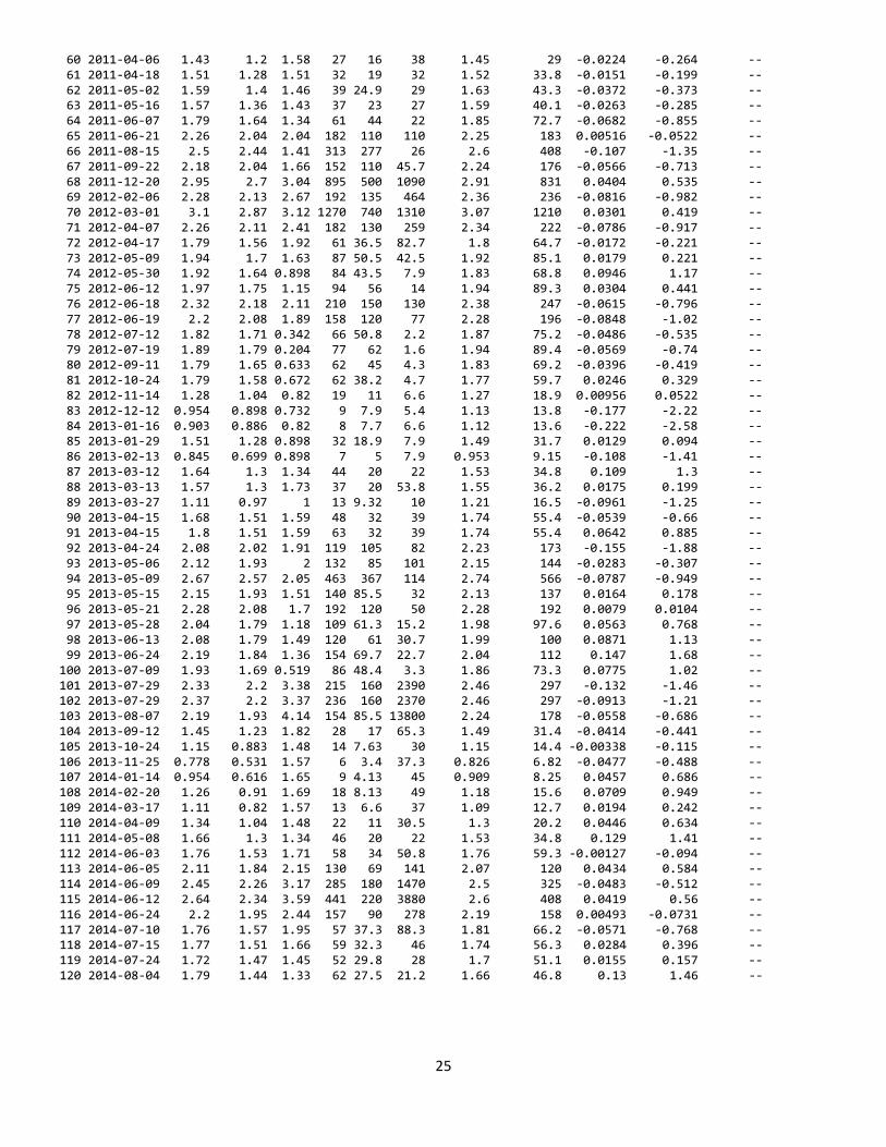
60 2011-04-06 1.43 1.2 1.58 27 16 38 1.45 29 -0.0224 -0.264 -- 61 2011-04-18 1.51 1.28 1.51 32 19 32 1.52 33.8 -0.0151 -0.199 -- 62 2011-05-02 1.59 1.4 1.46 39 24.9 29 1.63 43.3 -0.0372 -0.373 -- 63 2011-05-16 1.57 1.36 1.43 37 23 27 1.59 40.1 -0.0263 -0.285 -- 64 2011-06-07 1.79 1.64 1.34 61 44 22 1.85 72.7 -0.0682 -0.855 -- 65 2011-06-21 2.26 2.04 2.04 182 110 110 2.25 183 0.00516 -0.0522 -- 66 2011-08-15 2.5 2.44 1.41 313 277 26 2.6 408 -0.107 -1.35 -- 67 2011-09-22 2.18 2.04 1.66 152 110 45.7 2.24 176 -0.0566 -0.713 -- 68 2011-12-20 2.95 2.7 3.04 895 500 1090 2.91 831 0.0404 0.535 -- 69 2012-02-06 2.28 2.13 2.67 192 135 464 2.36 236 -0.0816 -0.982 -- 70 2012-03-01 3.1 2.87 3.12 1270 740 1310 3.07 1210 0.0301 0.419 -- 71 2012-04-07 2.26 2.11 2.41 182 130 259 2.34 222 -0.0786 -0.917 -- 72 2012-04-17 1.79 1.56 1.92 61 36.5 82.7 1.8 64.7 -0.0172 -0.221 -- 73 2012-05-09 1.94 1.7 1.63 87 50.5 42.5 1.92 85.1 0.0179 0.221 -- 74 2012-05-30 1.92 1.64 0.898 84 43.5 7.9 1.83 68.8 0.0946 1.17 -- 75 2012-06-12 1.97 1.75 1.15 94 56 14 1.94 89.3 0.0304 0.441 -- 76 2012-06-18 2.32 2.18 2.11 210 150 130 2.38 247 -0.0615 -0.796 -- 77 2012-06-19 2.2 2.08 1.89 158 120 77 2.28 196 -0.0848 -1.02 -- 78 2012-07-12 1.82 1.71 0.342 66 50.8 2.2 1.87 75.2 -0.0486 -0.535 -- 79 2012-07-19 1.89 1.79 0.204 77 62 1.6 1.94 89.4 -0.0569 -0.74 -- 80 2012-09-11 1.79 1.65 0.633 62 45 4.3 1.83 69.2 -0.0396 -0.419 -- 81 2012-10-24 1.79 1.58 0.672 62 38.2 4.7 1.77 59.7 0.0246 0.329 -- 82 2012-11-14 1.28 1.04 0.82 19 11 6.6 1.27 18.9 0.00956 0.0522 -- 83 2012-12-12 0.954 0.898 0.732 9 7.9 5.4 1.13 13.8 -0.177 -2.22 -- 84 2013-01-16 0.903 0.886 0.82 8 7.7 6.6 1.12 13.6 -0.222 -2.58 -- 85 2013-01-29 1.51 1.28 0.898 32 18.9 7.9 1.49 31.7 0.0129 0.094 -- 86 2013-02-13 0.845 0.699 0.898 7 5 7.9 0.953 9.15 -0.108 -1.41 -- 87 2013-03-12 1.64 1.3 1.34 44 20 22 1.53 34.8 0.109 1.3 -- 88 2013-03-13 1.57 1.3 1.73 37 20 53.8 1.55 36.2 0.0175 0.199 -- 89 2013-03-27 1.11 0.97 1 13 9.32 10 1.21 16.5 -0.0961 -1.25 -- 90 2013-04-15 1.68 1.51 1.59 48 32 39 1.74 55.4 -0.0539 -0.66 -- 91 2013-04-15 1.8 1.51 1.59 63 32 39 1.74 55.4 0.0642 0.885 -- 92 2013-04-24 2.08 2.02 1.91 119 105 82 2.23 173 -0.155 -1.88 -- 93 2013-05-06 2.12 1.93 2 132 85 101 2.15 144 -0.0283 -0.307 -- 94 2013-05-09 2.67 2.57 2.05 463 367 114 2.74 566 -0.0787 -0.949 -- 95 2013-05-15 2.15 1.93 1.51 140 85.5 32 2.13 137 0.0164 0.178 -- 96 2013-05-21 2.28 2.08 1.7 192 120 50 2.28 192 0.0079 0.0104 -- 97 2013-05-28 2.04 1.79 1.18 109 61.3 15.2 1.98 97.6 0.0563 0.768 -- 98 2013-06-13 2.08 1.79 1.49 120 61 30.7 1.99 100 0.0871 1.13 -- 99 2013-06-24 2.19 1.84 1.36 154 69.7 22.7 2.04 112 0.147 1.68 -- 100 2013-07-09 1.93 1.69 0.519 86 48.4 3.3 1.86 73.3 0.0775 1.02 -- 101 2013-07-29 2.33 2.2 3.38 215 160 2390 2.46 297 -0.132 -1.46 -- 102 2013-07-29 2.37 2.2 3.37 236 160 2370 2.46 297 -0.0913 -1.21 -- 103 2013-08-07 2.19 1.93 4.14 154 85.5 13800 2.24 178 -0.0558 -0.686 -- 104 2013-09-12 1.45 1.23 1.82 28 17 65.3 1.49 31.4 -0.0414 -0.441 -- 105 2013-10-24 1.15 0.883 1.48 14 7.63 30 1.15 14.4 -0.00338 -0.115 -- 106 2013-11-25 0.778 0.531 1.57 6 3.4 37.3 0.826 6.82 -0.0477 -0.488 -- 107 2014-01-14 0.954 0.616 1.65 9 4.13 45 0.909 8.25 0.0457 0.686 -- 108 2014-02-20 1.26 0.91 1.69 18 8.13 49 1.18 15.6 0.0709 0.949 -- 109 2014-03-17 1.11 0.82 1.57 13 6.6 37 1.09 12.7 0.0194 0.242 -- 110 2014-04-09 1.34 1.04 1.48 22 11 30.5 1.3 20.2 0.0446 0.634 -- 111 2014-05-08 1.66 1.3 1.34 46 20 22 1.53 34.8 0.129 1.41 -- 112 2014-06-03 1.76 1.53 1.71 58 34 50.8 1.76 59.3 -0.00127 -0.094 -- 113 2014-06-05 2.11 1.84 2.15 130 69 141 2.07 120 0.0434 0.584 -- 114 2014-06-09 2.45 2.26 3.17 285 180 1470 2.5 325 -0.0483 -0.512 -- 115 2014-06-12 2.64 2.34 3.59 441 220 3880 2.6 408 0.0419 0.56 -- 116 2014-06-24 2.2 1.95 2.44 157 90 278 2.19 158 0.00493 -0.0731 -- 117 2014-07-10 1.76 1.57 1.95 57 37.3 88.3 1.81 66.2 -0.0571 -0.768 -- 118 2014-07-15 1.77 1.51 1.66 59 32.3 46 1.74 56.3 0.0284 0.396 -- 119 2014-07-24 1.72 1.47 1.45 52 29.8 28 1.7 51.1 0.0155 0.157 -- 120 2014-08-04 1.79 1.44 1.33 62 27.5 21.2 1.66 46.8 0.13 1.46 --

26

Definitions SSC: Suspended-sediment concentration (SSC) in mg/L (80154) TURB: Turbidity in FNU (63680) Q: Streamflow, in ft3/s (00060)

27

Attachment C. Example Model Archive Summary for an Acoustic Suspended Sediment Model

Model Archive Summary for Suspended-Sediment Concentration at Station 01648010; Rock Creek at Joyce Road at Washington, DC

This model archive summary documents the suspended-sediment concentration (SSC) model developed to compute 15-minute SSC for the U.S. Geological Survey (USGS) station, Rock Creek at Joyce Road (USGS ID: 01648010) from October 1, 2014 onward. This is the first model developed for the site to compute continuous SSC. The methods used follow USGS guidance as referenced in relevant Office of Surface Water/Office of Water Quality Technical Memoranda and USGS Techniques and Methods, book 3, chap. C5 (Landers and others, 2016).

Site and Model Information Site number: 01648010 Site name: Rock Creek at Joyce Rd, Washington, DC Location: Lat 38°57'36.6", long 77°02'31.4" (NAD 1927), Washington, DC, Hydrologic Unit: 02070010, on right bank at downstream side of bridge on Joyce Road. Drainage area: 62.7 mi2

Model number: 01648010.SSC.WY15.1

Date model was created: September 9, 2016 Model calibration data period: October 8, 2014 to May 03, 2016 Model application date: October 8, 2014 onwards Computed by: Joseph Bell, USGS, MD.DE.DC WSC (jmbell@usgs.gov) Reviewed by: Timothy Straub, USGS, IL-IA WSC (tdstraub@usgs.gov), and Mark Landers, USGS, OSW (landers@usgs.gov) Approved by: USGS, Center Director, MD.DE.DC Water Science Center

Model Data

All model data were collected using USGS protocols described in Edwards and Glysson (1999), Landers and others (2016), and the USGS National Field Manual. All data are stored in the National Water Information System (NWIS) database (http://dx.doi.org/10.5066/F7P55KJN).

Suspended sediment characteristics at this site are computed from a regression model based on measured suspended sediment characteristics and sediment-corrected backscatter (𝑆𝑆𝑇������). The regression model is based on 41 concurrent measurements of SSC and 𝑆𝑆𝑇������ collected from October 8, 2014, through May 3, 2016. An additional 51 concurrent data sets collected during this period were evaluated and excluded from the regression because of potential serial correlation of auto sampler results, and are flagged as excluded in the

28

model calibration dataset. Samples represent the range of observed hydrologic, sediment, and acoustic conditions.

Rock Creek at Joyce Road is a Piedmont valley stream that bisects Rock Creek Park from the border of Washington D.C. south to the Potomac River and ultimately into the Chesapeake Bay, draining a heavily urbanized watershed. The median and maximum SSC in the calibration data set is 84 and 2,900 mg/L, respectively. The system is dominated by fine size material. The average and standard deviation of the percent of fine sized material is 83% and 12%, respectively from 98 samples. Summary statistics and complete model-calibration dataset are provided in the model statistics.

Sediment Data

Discrete, manual sample collection for SSC monitoring takes place on a 4-week, fixed-frequency (FF) interval and targets 10–12 unique storm events throughout the year. These samples are collected by trained USGS personnel using DH-81, DH-95, or D-95 suspended-sediment samplers as dictated by in-stream conditions. When conditions are safe for wading, the equal-width-increment (EWI) method is used to collect a sample from a cross-section approximately 75ft downstream of the Joyce Rd Bridge; these samples typically are composited for analysis. When conditions are not safe for wading, the EWI method is used to collect a sample from the downstream side of the Joyce Rd Bridge. There are no appreciable inputs between the Joyce Rd Bridge and wading cross section.

Discrete monitoring is augmented by the use of an automatic sampler to facilitate sampling during 8-12 storm events throughout the year. The automatic sampler is configured to trigger when empirically-determined threshold(s) are exceeded and paced to collect 4 samples across a given storm hydrograph. Storm-sampling efforts target rising, peak, and falling stream conditions throughout the year to capture the range of sediment, flow, and seasonal conditions. To avoid imparting a negative bias on SSC results, SSC samples are not drawn from a churn splitter. All samples are analyzed for SSC in the USGS Sediment Laboratory in Louisville, Kentucky.

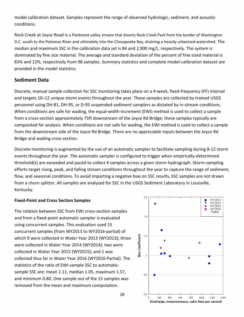
Fixed-Point and Cross Section Samples

The relation between SSC from EWI cross-section samples and from a fixed-point automatic sampler is evaluated using concurrent samples. This evaluation used 15 concurrent samples (from WY2013 to WY2016-partial) of which 9 were collected in Water Year 2013 (WY2013); three were collected in Water Year 2014 (WY2014); two were collected in Water Year 2015 (WY2015); and 1 was collected thus far in Water Year 2016 (WY2016 Partial). The statistics of the ratio of EWI-sample SSC to automatic-sample SSC are: mean 1.11, median 1.05, maximum 1.57, and minimum 0.80. One sample out of the 15 samples was removed from the mean and maximum computation.

29

Additionally, results from a replicate sample were used for ratio analysis on April 20, 2013. This replicate was ordered based on field-crew concerns about digging the sampler into the bed during collection; the ratio affiliated with the environmental sample is 2.12, and the ratio for the replicate sample is 1.02. Seventy-one percent of the ratios are within 0.9 and 1.1, and 79 percent are within 0.8 and 1.2. A plot of box coefficients versus streamflow indicates scatter about the 1.0 axis (see adjacent plot). A constant ratio of EWI cross-section to automatic-sampler SSC appears reasonable for this site for WY2013−2015. All single-station samples were multiplied by a coefficient (box coefficient) of 1.00 to adjust to cross-section concentration.

Surrogate Data

At the Joyce Rd Bridge, a SonTek Argonaut SL ADVM (for sediment-acoustic index method) and automatic-sampler intake are installed. The ADVM is mounted on the face of the right bridge abutment, near the middle of the bridge. The beams are horizontal and perpendicular to the flow. The gage house is located downstream of the bridge and on the right bank. Power from the gage house is regulated and fused to provide a constant, fixed 13.5 volts to the ADVM. Backup power (also regulated) is provided by a regulated 40-watt solar panel charging a 12-volt deep-cycle battery.

For the period 08/01/2015-08/06/2015 ADVM data were degraded due to an atypical, large sandbar migrating through the cross section. This bar was the result of accelerated bank erosion associated with the large root-ball failure of a ~75ft oak tree located along the left bank, approximate 1/4 mi upstream of the Joyce Rd Bridge.

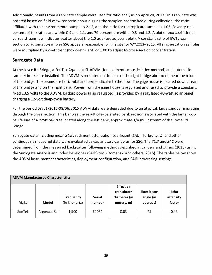
Surrogate data including mean 𝑆𝑆𝑇������, sediment attenuation coefficient (SAC), Turbidity, Q, and other continuously measured data were evaluated as explanatory variables for SSC. The 𝑆𝑆𝑇������ and SAC were determined from the measured backscatter following methods described in Landers and others (2016) using the Surrogate Analysis and Index Developer (SAID) tool (Domanski and others, 2015). The tables below show the ADVM instrument characteristics, deployment configuration, and SAID processing settings.

ADVM Manufactured Characteristics

Make Model Frequency

(in kilohertz) Serial

number

Effective transducer

diameter (in meters, m)

Slant beam angle (in degrees)

Echo intensity

factor

SonTek Argonaut SL 1,500 E2064 0.03 25 0.43

30

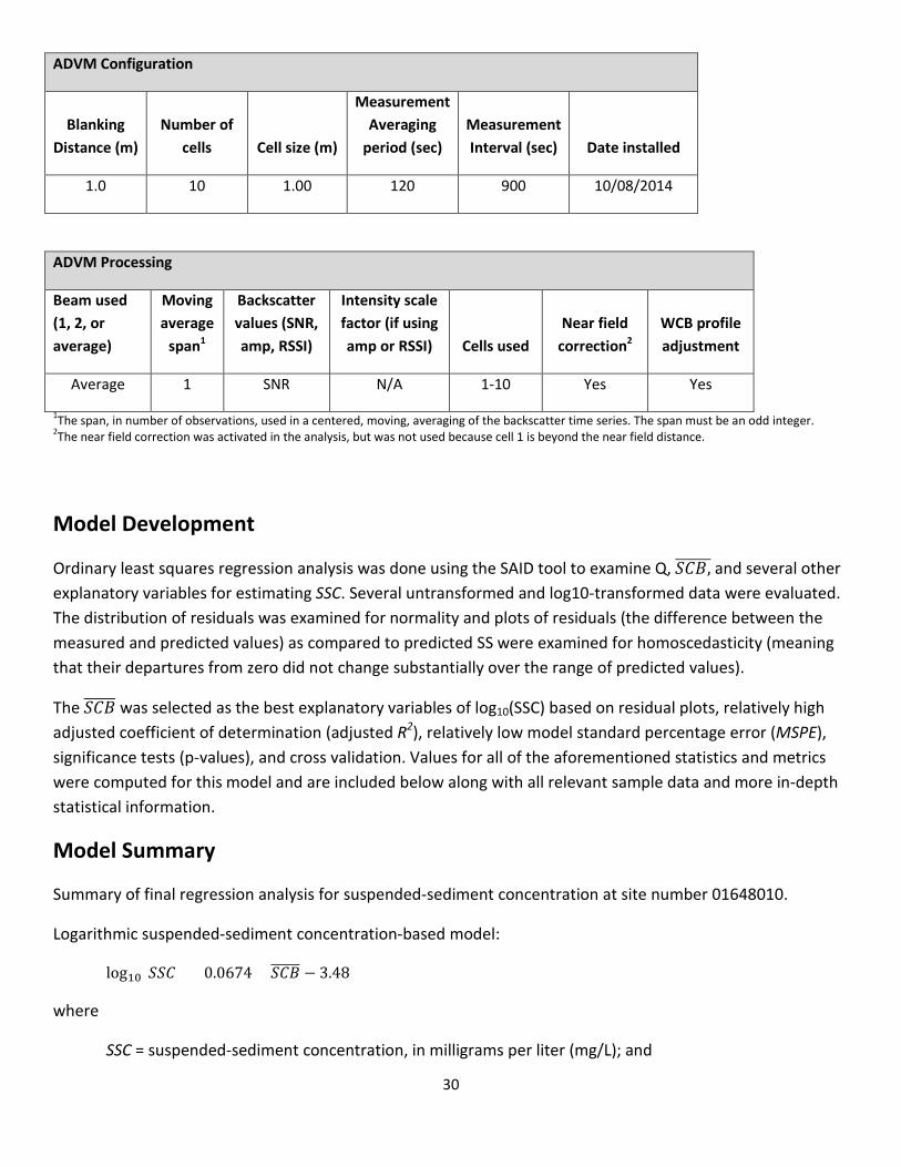
ADVM Configuration

Blanking Distance (m)

Number of cells Cell size (m)

Measurement Averaging

period (sec) Measurement Interval (sec) Date installed

1.0 10 1.00 120 900 10/08/2014

ADVM Processing

Beam used (1, 2, or average)

Moving average

span1

Backscatter values (SNR, amp, RSSI)

Intensity scale factor (if using amp or RSSI) Cells used

Near field correction2

WCB profile adjustment

Average 1 SNR N/A 1-10 Yes Yes

1The span, in number of observations, used in a centered, moving, averaging of the backscatter time series. The span must be an odd integer. 2The near field correction was activated in the analysis, but was not used because cell 1 is beyond the near field distance.

Model Development

Ordinary least squares regression analysis was done using the SAID tool to examine Q, 𝑆𝑆𝑇,������ and several other explanatory variables for estimating SSC. Several untransformed and log10-transformed data were evaluated. The distribution of residuals was examined for normality and plots of residuals (the difference between the measured and predicted values) as compared to predicted SS were examined for homoscedasticity (meaning that their departures from zero did not change substantially over the range of predicted values).

The 𝑆𝑆𝑇������ was selected as the best explanatory variables of log10(SSC) based on residual plots, relatively high adjusted coefficient of determination (adjusted R2), relatively low model standard percentage error (MSPE), significance tests (p-values), and cross validation. Values for all of the aforementioned statistics and metrics were computed for this model and are included below along with all relevant sample data and more in-depth statistical information.

Model Summary

Summary of final regression analysis for suspended-sediment concentration at site number 01648010.

Logarithmic suspended-sediment concentration-based model:

log10(𝑆𝑆𝑆) = 0.0674 × 𝑆𝑆𝑇������ − 3.48

where

SSC = suspended-sediment concentration, in milligrams per liter (mg/L); and

31

𝑆𝑆𝑇������ = sediment corrected backscatter in decibels.

The use of 𝑆𝑆𝑇������ as an explanatory variable for SSC is appropriate physically and statistically. Physically, 𝑆𝑆𝑇������ varies linearly with log10(SSC) following basic principles of acoustic scattering. Changing sediment particle sizes for a given concentration can produce additional variance in 𝑆𝑆𝑇������, but those changes are negligible at this site.

The log-transformed model may be retransformed to the original units so that SSC can be calculated directly. The retransformation introduces a bias in the calculated constituent. This bias may be corrected using Duan’s Bias Correction Factor (BCF). For this model, the calculated BCF is 1.22. The retransformed model, accounting for BCF is:

Model Start date End date

Linear Regression Model

1 10/08/2014 Current 𝑆𝑆𝑆 = 𝑆𝑆𝑇������0.0674 × 10−3.48 × 1.22

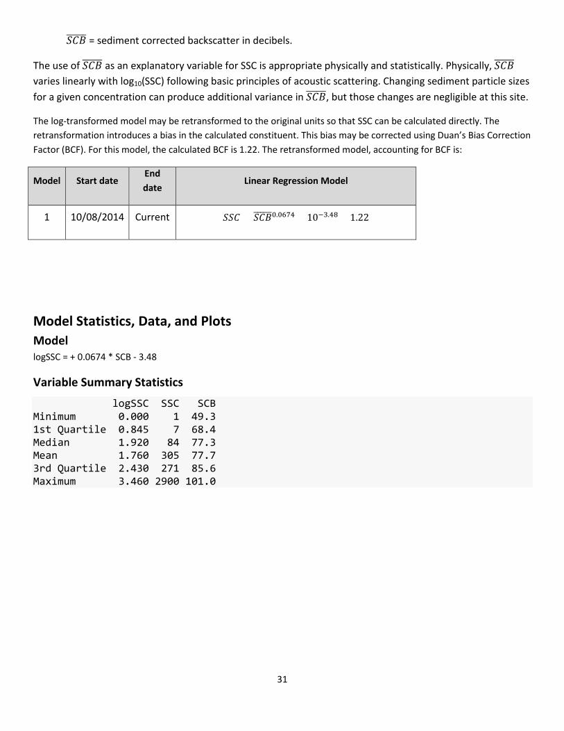
Model Statistics, Data, and Plots Model logSSC = + 0.0674 * SCB - 3.48

Variable Summary Statistics

logSSC SSC SCB Minimum 0.000 1 49.3 1st Quartile 0.845 7 68.4 Median 1.920 84 77.3 Mean 1.760 305 77.7 3rd Quartile 2.430 271 85.6 Maximum 3.460 2900 101.0

32

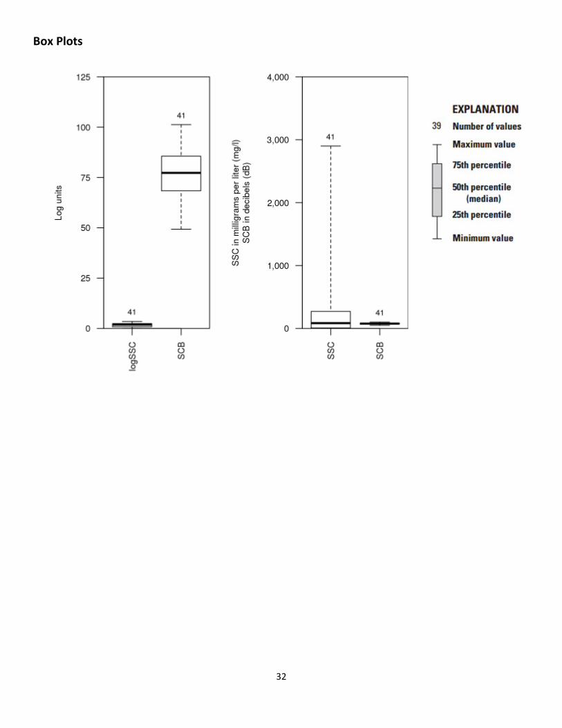
Box Plots

33

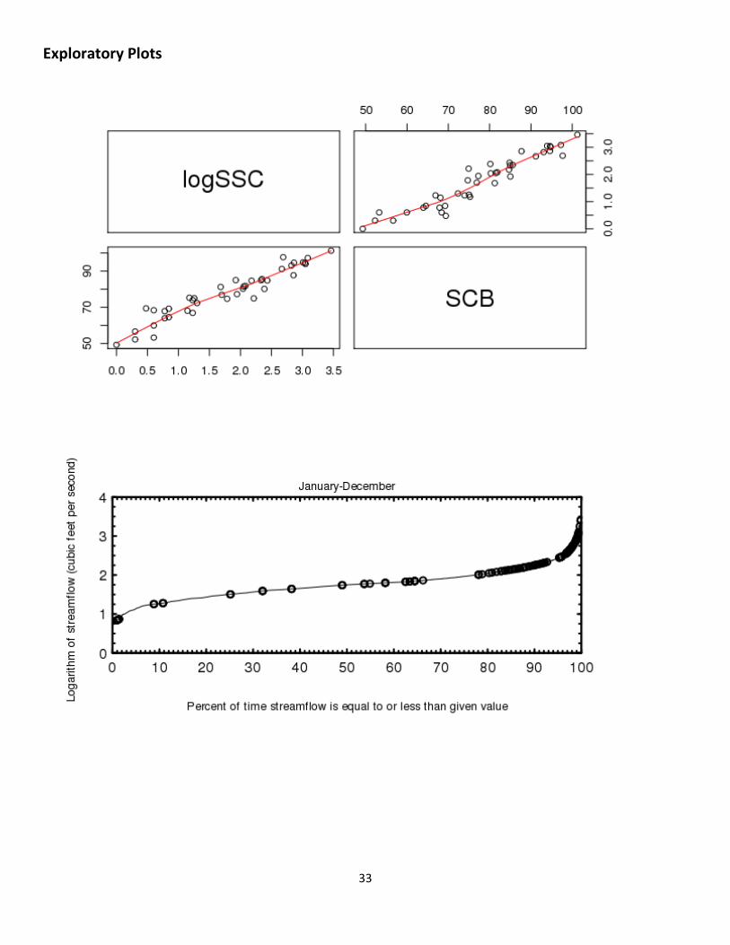
Exploratory Plots

34

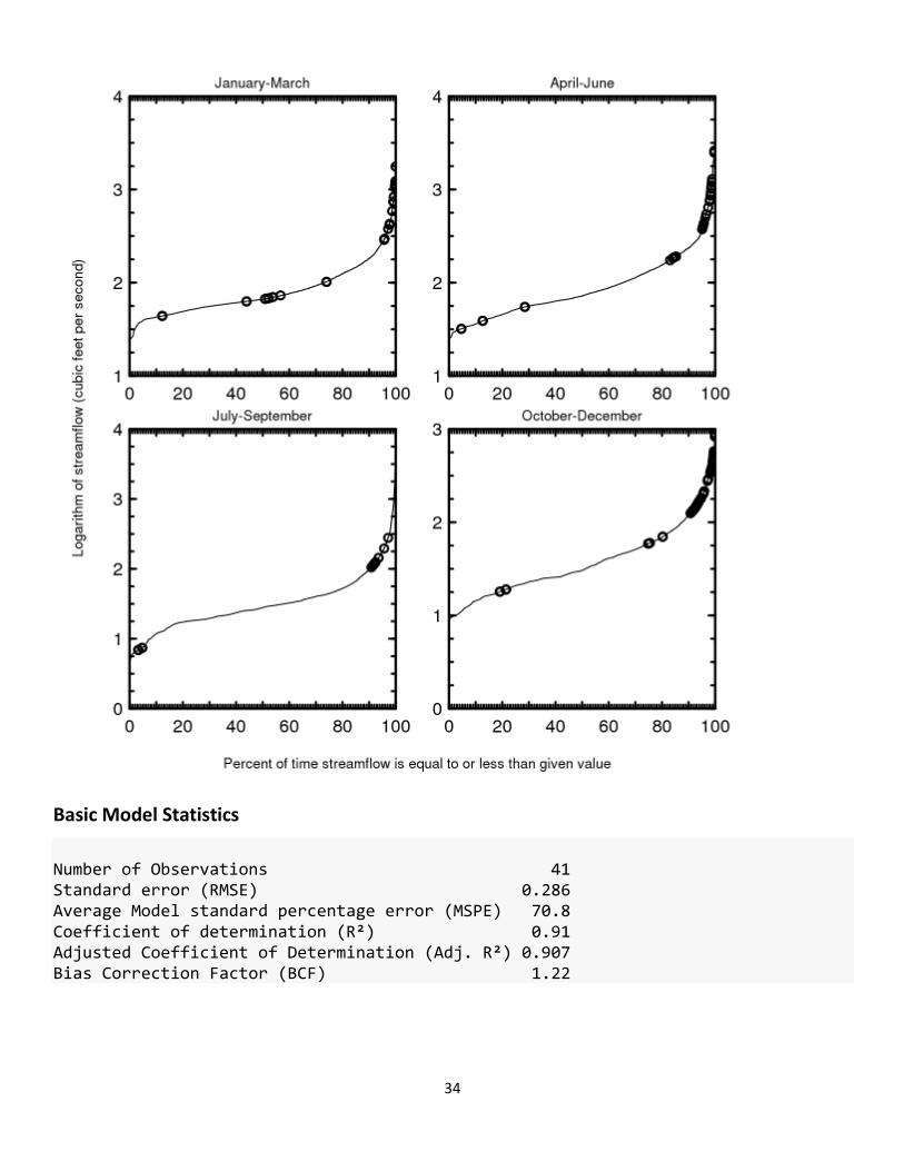
Basic Model Statistics

Number of Observations 41 Standard error (RMSE) 0.286 Average Model standard percentage error (MSPE) 70.8 Coefficient of determination (R²) 0.91 Adjusted Coefficient of Determination (Adj. R²) 0.907 Bias Correction Factor (BCF) 1.22

35

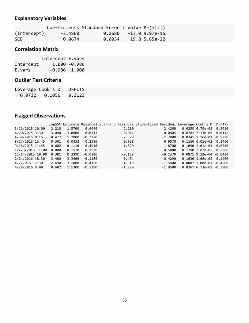
Explanatory Variables

Coefficients Standard Error t value Pr(>|t|) (Intercept) -3.4800 0.2680 -13.0 9.97e-16 SCB 0.0674 0.0034 19.8 5.85e-22

Correlation Matrix

Intercept E.vars Intercept 1.000 -0.986 E.vars -0.986 1.000

Outlier Test Criteria

Leverage Cook's D DFFITS 0.0732 0.1056 0.3123

Flagged Observations logSSC Estimate Residual Standard Residual Studentized Residual Leverage Cook's D DFFITS 3/11/2015 10:00 2.210 1.5700 0.6440 2.280 2.4200 0.0255 6.79e-02 0.3910 4/20/2015 3:30 3.090 3.0800 0.0113 0.041 0.0405 0.0782 7.13e-05 0.0118 4/30/2015 8:15 0.477 1.2000 -0.7220 -2.570 -2.7800 0.0341 1.16e-01 -0.5220 8/27/2015 13:45 0.301 0.0432 0.2580 0.958 0.9570 0.1160 6.01e-02 0.3460 9/16/2015 11:45 0.602 0.1110 0.4910 1.820 1.8700 0.1090 2.01e-01 0.6540 11/23/2015 11:00 0.000 -0.1570 0.1570 0.593 0.5880 0.1390 2.82e-02 0.2360 12/14/2015 10:00 0.301 0.3390 -0.0380 -0.139 -0.1370 0.0871 9.22e-04 -0.0424 2/24/2016 18:30 3.460 3.3400 0.1180 0.434 0.4290 0.1030 1.08e-02 0.1450 4/7/2016 17:30 2.690 3.1000 -0.4150 -1.510 -1.5400 0.0807 1.00e-01 -0.4560 4/26/2016 9:00 0.602 1.1300 -0.5290 -1.880 -1.9500 0.0367 6.73e-02 -0.3800

36

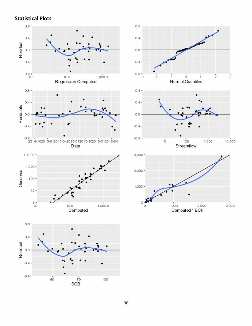
Statistical Plots

37

38

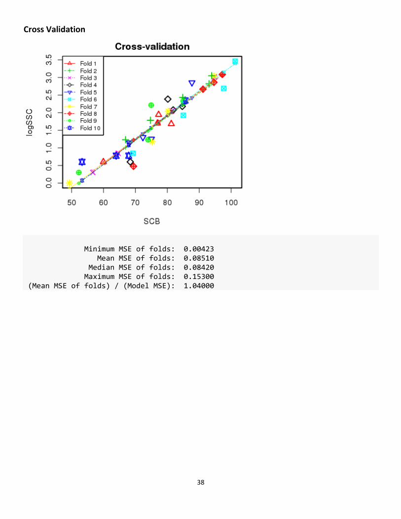
Cross Validation

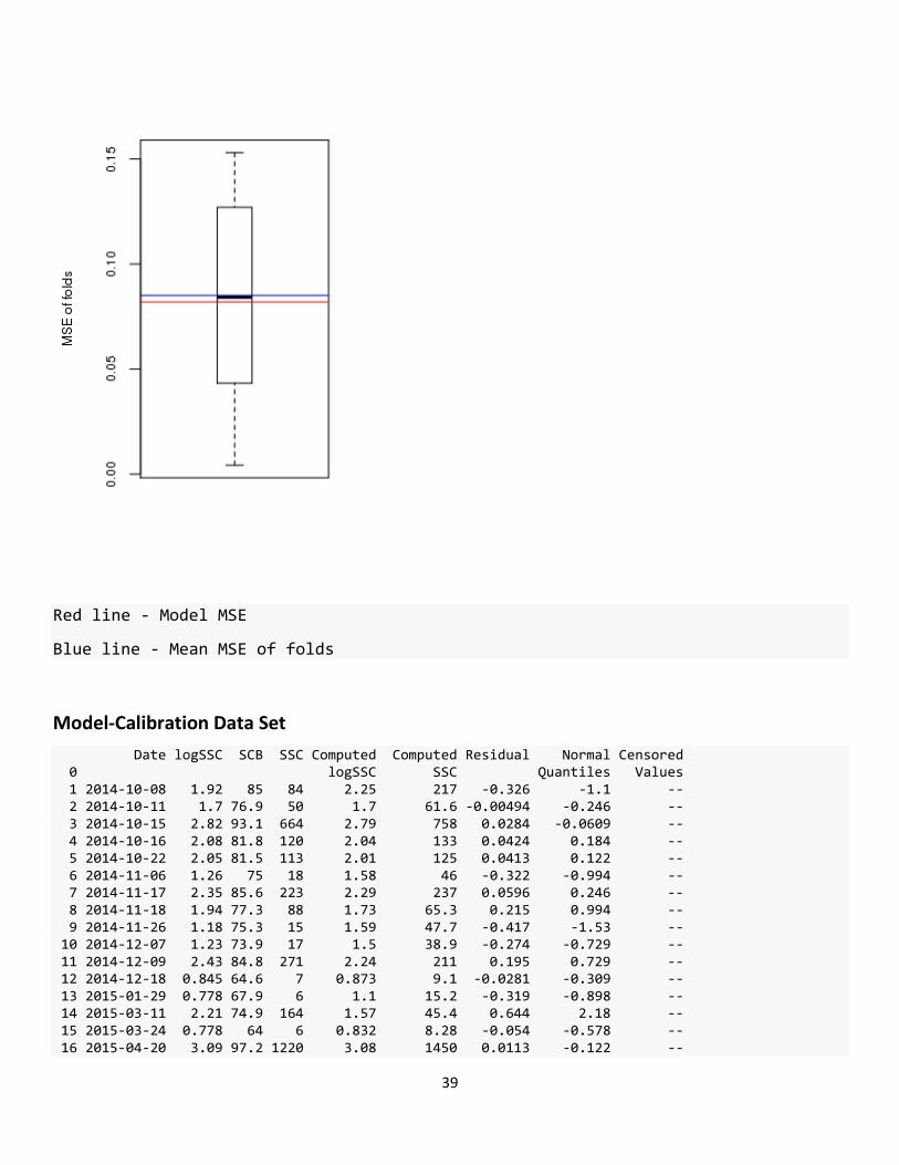
Minimum MSE of folds: 0.00423 Mean MSE of folds: 0.08510 Median MSE of folds: 0.08420 Maximum MSE of folds: 0.15300 (Mean MSE of folds) / (Model MSE): 1.04000

39

Red line - Model MSE

Blue line - Mean MSE of folds

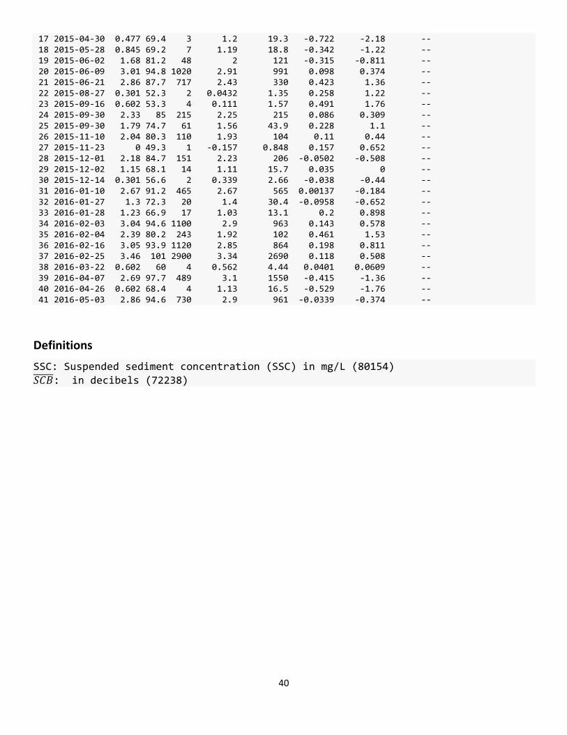
Model-Calibration Data Set Date logSSC SCB SSC Computed Computed Residual Normal Censored 0 logSSC SSC Quantiles Values 1 2014-10-08 1.92 85 84 2.25 217 -0.326 -1.1 -- 2 2014-10-11 1.7 76.9 50 1.7 61.6 -0.00494 -0.246 -- 3 2014-10-15 2.82 93.1 664 2.79 758 0.0284 -0.0609 -- 4 2014-10-16 2.08 81.8 120 2.04 133 0.0424 0.184 -- 5 2014-10-22 2.05 81.5 113 2.01 125 0.0413 0.122 -- 6 2014-11-06 1.26 75 18 1.58 46 -0.322 -0.994 -- 7 2014-11-17 2.35 85.6 223 2.29 237 0.0596 0.246 -- 8 2014-11-18 1.94 77.3 88 1.73 65.3 0.215 0.994 -- 9 2014-11-26 1.18 75.3 15 1.59 47.7 -0.417 -1.53 -- 10 2014-12-07 1.23 73.9 17 1.5 38.9 -0.274 -0.729 -- 11 2014-12-09 2.43 84.8 271 2.24 211 0.195 0.729 -- 12 2014-12-18 0.845 64.6 7 0.873 9.1 -0.0281 -0.309 -- 13 2015-01-29 0.778 67.9 6 1.1 15.2 -0.319 -0.898 -- 14 2015-03-11 2.21 74.9 164 1.57 45.4 0.644 2.18 -- 15 2015-03-24 0.778 64 6 0.832 8.28 -0.054 -0.578 -- 16 2015-04-20 3.09 97.2 1220 3.08 1450 0.0113 -0.122 --

40

17 2015-04-30 0.477 69.4 3 1.2 19.3 -0.722 -2.18 -- 18 2015-05-28 0.845 69.2 7 1.19 18.8 -0.342 -1.22 -- 19 2015-06-02 1.68 81.2 48 2 121 -0.315 -0.811 -- 20 2015-06-09 3.01 94.8 1020 2.91 991 0.098 0.374 -- 21 2015-06-21 2.86 87.7 717 2.43 330 0.423 1.36 -- 22 2015-08-27 0.301 52.3 2 0.0432 1.35 0.258 1.22 -- 23 2015-09-16 0.602 53.3 4 0.111 1.57 0.491 1.76 -- 24 2015-09-30 2.33 85 215 2.25 215 0.086 0.309 -- 25 2015-09-30 1.79 74.7 61 1.56 43.9 0.228 1.1 -- 26 2015-11-10 2.04 80.3 110 1.93 104 0.11 0.44 -- 27 2015-11-23 0 49.3 1 -0.157 0.848 0.157 0.652 -- 28 2015-12-01 2.18 84.7 151 2.23 206 -0.0502 -0.508 -- 29 2015-12-02 1.15 68.1 14 1.11 15.7 0.035 0 -- 30 2015-12-14 0.301 56.6 2 0.339 2.66 -0.038 -0.44 -- 31 2016-01-10 2.67 91.2 465 2.67 565 0.00137 -0.184 -- 32 2016-01-27 1.3 72.3 20 1.4 30.4 -0.0958 -0.652 -- 33 2016-01-28 1.23 66.9 17 1.03 13.1 0.2 0.898 -- 34 2016-02-03 3.04 94.6 1100 2.9 963 0.143 0.578 -- 35 2016-02-04 2.39 80.2 243 1.92 102 0.461 1.53 -- 36 2016-02-16 3.05 93.9 1120 2.85 864 0.198 0.811 -- 37 2016-02-25 3.46 101 2900 3.34 2690 0.118 0.508 -- 38 2016-03-22 0.602 60 4 0.562 4.44 0.0401 0.0609 -- 39 2016-04-07 2.69 97.7 489 3.1 1550 -0.415 -1.36 -- 40 2016-04-26 0.602 68.4 4 1.13 16.5 -0.529 -1.76 -- 41 2016-05-03 2.86 94.6 730 2.9 961 -0.0339 -0.374 --

Definitions

SSC: Suspended sediment concentration (SSC) in mg/L (80154) 𝑆𝑆𝑇������: in decibels (72238)