united states epa 640-c-09-003 and toxic substances ...€¦ · endocrine disruptor screening...

United States Environmental Protection Agency

Prevention, Pesticides and Toxic Substances (7101)

EPA 640-C-09-003 October 2009

Endocrine Disruptor Screening Program Test Guidelines

OPPTS 890.1150:

Androgen Receptor Binding (Rat Prostate Cytosol)

NOTICE

This guideline is one of a series of test guidelines established by the Office of Prevention, Pesticides and Toxic Substances (OPPTS), United States Environmental Protection Agency for use in testing pesticides and chemical substances to develop data for submission to the Agency under the Toxic Substances Control Act (TSCA) (15 U.S.C. 2601, et seq.), the Federal Insecticide, Fungicide and Rodenticide Act (FIFRA) (7 U.S.C. 136, et seq.), and section 408 of the Federal Food, Drug and Cosmetic (FFDCA) (21 U.S.C. 346a). The OPPTS test guidelines serve as a compendium of accepted scientific methodologies and protocols that are intended to provide data to inform regulatory decisions under TSCA, FIFRA, and/or FFDCA. This document provides guidance for conducting the test, and is also used by EPA, the public, and the companies that are subject to data submission requirements under TSCA, FIFRA and/or the FFDCA. As a guidance document, these guidelines are not binding on either EPA or any outside parties, and the EPA may depart from the guidelines where circumstances warrant and without prior notice. The procedures contained in this guideline are strongly recommended for generating the data that are the subject of the guideline, but EPA recognizes that departures may be appropriate in specific situations. You may propose alternatives to the recommendations described in these guidelines, and the Agency will assess them for appropriateness on a case-by-case basis. For additional information about OPPTS harmonized test guidelines and to access the guidelines electronically, please go to http://www.epa.gov/oppts and select “Test Methods & Guidelines” on the left side navigation menu. You may also access the guidelines in http://www.regulations.gov grouped by Series under Docket ID #s: EPA-HQ-OPPT-2009-0150 through EPA-HQ-OPPT-2009-0159, and EPA-HQ-OPPT-2009-0576.

http://www.regulations.gov/

OPPTS 890.1150: Androgen Receptor Binding (Rat Prostate Cytosol) (a) Scope.

(1) Applicability. This guideline is intended to meet testing requirements of the Toxic Substances Control Act (TSCA) (15 U.S.C. 2601, et seq.), the Federal Insecticide, Fungicide, and Rodenticide Act (FIFRA) (7 U.S.C. 136, et seq.), and the Federal Food, Drug, and Cosmetic Act (FFDCA) (21 U.S.C. 346a).

(2) Background. The Endocrine Disruptor Screening Program (EDSP)

reflects a two-tiered approach to implement the statutory testing requirements of FFDCA section 408(p) (21 U.S.C. 346a). In general, EPA intends to use the data collected under the EDSP, along with other information, to determine if a pesticide chemical, or other substances, may pose a risk to human health or the environment due to disruption of the endocrine system.

This test guideline is intended to be used in conjunction with other

guidelines in the OPPTS 890 series that make up the full screening battery under the EDSP to identify substances that have the potential to interact with the estrogen, androgen, or thyroid hormone (Tier 1 “screening”). The determination will be made on a weight-of-evidence basis taking into account data from the Tier 1 assays and other scientifically relevant information available. The fact that a substance may interact with a hormone system, however, does not mean that when the substance is used, it will cause adverse effects in humans or ecological systems.

Chemicals that go through Tier 1 screening and are found to have the

potential to interact with the estrogen, androgen, or thyroid hormone systems will proceed to the next stage of the EDSP where EPA will determine which, if any, of the Tier 2 tests are necessary based on the available data. Tier 2 testing is designed to identify any adverse endocrine-related effects caused by the substance, and establish a quantitative relationship between the dose and that endocrine effect.

(b) Purpose. Determine ability of compound to compete with [3H] ligand for binding

in rat ventral prostate tissue homogenate. (c) General Experimental Design.

(1) Safety and Operating Precautions. Follow the regulations and procedures as described in the Hazardous Agent Protocol and in the Radiation Safety Manual and Protocols for US EPA for all procedures with radioisotopes.

Page 1

(2) Animal Use. Follow U.S. EPA approved animal use protocols.

(3) Equipment and Materials.

(i) Equipment.

Corning Stir/hot Plates Pipetters Balance Metzenbaum scissors Polytron PT 35/10 Tissue Homogenizer Vacuum Concentrator Refrigerated General Laboratory Centrifuge High-Speed Refrigerated Centrifuge (up to 30,000 x g) pH Meter with Tris Compatible Electrode Scintillation Counter Refrigerators

(ii) Chemicals.

Tris HCL & Tris Base Phenylmethylsulfonyl Fluoride (PMSF) Glycerol 99%+ Sodium Molybdate Ethylenediaminetetraacetic acid (EDTA); Disodium salt Dithiothreitol (DTT) Potassium Chloride Hydroxyapatite (HAP; BIO-RAD) Scintillation Cocktail (Flow Scint III) Ethyl Alcohol, anhydrous [3H]-R1881 (NEN; Purity >97%; 1 mCi/ml, specific activity 70-87

Ci/mmol) Radioinert R1881 (NEN; MW 284.4,) Triamcinolone Acetonide Steroids (Steraloids - recrystallized) Optifluor

(iii) Supplies.

20 ml Polypropylene Scintillation Vials 12 x 75 mm Borosilicate Glass Test Tubes

Page 2

1000 ml graduated cylinders 500 ml Erlenmeyer flasks Pipette tips

(4) Stock Preparations.

(i) Preparation of Stock Solutions for Making Low-Salt TEDG

Buffer.

EDTA Stock Solution. Add 7.444g disodium EDTA to 100 ml ddH2O = 200mM. Store at 4°C. Use 750 µl/100 ml TEDG buffer = 1.5 mM.

PMSF Stock Solution. Add 1.742 g PMSF to 100 ml ethanol = 100 mM. Store at 4°C. Use 1.00 ml/100ml TEDG buffer = 1.0 mM.

Sodium Molybdate Stock. Add 2.419 g sodium molybdate to 8.0 ml ddH2O in a 10 ml volumetric flask; bring the total volume to 10 mls = 1.0 M. Store at 4°C. Use 100 µl /100 ml TEDG buffer = 1.0 mM.

1 M Tris Buffer. Add 147.24 g Tris-HCL + 8.0 g Tris base to 800ml ddH2O in a volumetric flask; bring the final volume to 1.0 liter. Refrigerate to 4°C and pH (using 4°C pH standardizing solutions) the cooled solution to 7.4. Store at 4°C. Use 1.0 ml/100 ml TEDG buffer = 10mM. (50 mM Tris = 50 ml 1 M Tris/1 L ddH2O).

Potassium Chloride Stock Solution. Add 298.2 g KCL to 600 ml ddH2O in a 1000 ml volumetric flask; bring the total volume to 1000 ml = 4.0 M. Store at room temperature. Use 10.0 ml per 100 ml high-salt TEDG buffer = 0.4 M.

(ii) Preparation of Low-Salt TEDG Buffer (pH 7.4).

To make 100 ml of low-salt TEDG buffer add the following together

in this order: • 87.15 ml ddH2O • 1.0 ml 1M TRIS • 10.0 ml glycerol • 100 µl 1 M sodium molybdate • 7.50 µl 200mM EDTA • 1.0 ml 100mM PMSF • 15.4 mg DTT (add immediately before use, see below)

Check pH of the final solution to make sure it is 7.4 at 4°C. Add 15.4 mg DTT directly to 100 ml TEDG buffer the morning of the

receptor isolation = 1.0 mM DTT.

Page 3

(iii) Preparation of 50 mM TRIS Buffer for HAP Preparation. 50 mM TRIS Buffer is used to wash the Hydroxyapatite Slurry prepared in section below.

To prepare add 50.0 ml of 1.0 M TRIS to 950 ml ddH2O. Store at 4°C. Check pH of the final solution to make sure it is 7.4 at 4°C.

(iv) Preparation of 60% Hydroxyapatite (HAP) Slurry.

Shake BIO-RAD HT-GEL until all the HAP is in suspension (i.e.,

looks like milk). The evening before the receptor extraction, pour 100 ml (or an appropriate volume) into a 100 ml graduated cylinder, parafilm seal the top and place in the refrigerator for at least 2h.

Pour off the phosphate buffer supernatant, and bring the volume to 100 ml with 50 mM TRIS. Suspend the HAP by parafilm sealing the top of the graduated cylinder and inverting the cylinder several times. Place in the refrigerator overnight.

The next morning, wash HAP two (2) more times with fresh 50 mM TRIS buffer.

After the last wash, add enough 50 mM TRIS to make the final solution a 60% slurry (i.e., if the volume of the settled HAP is 60 ml bring the final volume of the slurry to 100 ml with 50 mM TRIS).

Store at 4°C until ready for use in the extraction.

(v) Preparation of [3H]-R1881 Stock Solutions.

Dilute the original 1.0 mCi/ml stock of [3H]-R1881 to 0.1 µM (i.e., 1 x 10-7 M). This is most easily accomplished by pipetting 1 µl of the stock solution for every specific activity unit (Ci/mmol) and diluting this to 10.0 ml with ethanol. Thus, if the specific activity of the stock vial is 86 Ci/mmol, then pipette 86.0 µl into an amber colored vial (i.e., R1881 is photosensitive) and add 10.0 ml ethanol to the vial; this solution is 1 x 10-7M. Note: Store [3H]-R1881 stock solution and dilutions at -20°C. Store stock solution in original protective vial and store dilutions in amber glass vials. This product is light-sensitive; minimize exposure to light. The recommended shelf life of [3H]-R1881 is 7 months past the manufacture date when stored at -20°C.

(vi) Calculation Check and Dilutions for [3H]-R1881 stock

solutions.

Page 4

The calculation below is based on the specific activity of the [3H]-R1881 stock given in the example above. The specific activity value may change based on the lot of radioligand obtained from the manufacturer, thus the calculation below is only an example:

Example Calculation

86 µl x 1.0 mCi/1000 µl = 86 x 10-3 mCi R1881 = 86 x 10-6 Ci R1881;

86 x 10-6 Ci ÷ 86.0 Ci/mmol = 1 x 10-6 mmol R1881 = 1 x 10-9 moles R1881;

1 x 10-9 moles R1881 ÷ 0.010 liters = 1 x 10-7 moles/liter = 0.1 µM = 1 x 10-7 M

To prepare the 1 x 10-8 M stock simply make a 10-fold dilution of

the 1 x 10-7 M stock (i.e., pipette 1.0 ml of the 1 x 10-7 M stock into a clean amber colored vial and add 9 ml ethanol = 0.01 µM).

(vii) Preparation of 100X Radioinert R1881 Solutions. The R1881

comes as a 5.00 mg quantity.

Dilute the original stock to 5.0 ml with ethanol (or alternate solvent if used with the test chemical) = 3.52 mM. Take 56.82 µl and dilute to 20 ml in an amber vial with ethanol (or alternate solvent) = 1 x 10-5 M R1881. This is the 10 µM radioinert R1881 stock.

To make the 1.0 µM radioinert R1881 stock, pipette 2 ml of the 10 µM stock into an amber vial and dilute to 20 ml with ethanol = 1 x 10-6M = 1.0 µM radioinert R1881 stock. To make the 0.10 µM radioinert R1881 stock, pipette 2 ml of the 1 µM stock into an amber vial and dilute to 20 ml with ethanol = 1 x 10-7M = 0.10 µM radioinert R1881 stock.

(vii) Solvent selection for Standard R1881 and Test Chemicals. Use

the same solvent to make up the Radioinert R1881 standard as the solvent selected for the test chemical being tested in a given run. The recommended solvent for this protocol is 100% ethanol, followed by water and DMSO. Once a chemical is dissolved in solvent, examine the tube carefully by visual inspection for evidence of precipitation. Observation under a dissecting scope or monitoring absorbance (650 nm) with a spectrophotometer are useful approaches for detecting precipitation. If precipitation is noted, it may be appropriate to try a different dilution scheme (e.g., starting from a lower stock concentration) or a different solvent. If the chemical is not soluble at the highest concentration recommended in the protocol, prepare a lower concentration of test

Page 5

chemical (e.g., ½ log lower) and test it. If a chemical is not soluble in ethanol, try to dissolve it in water or DMSO.

(ix) Radioinert R1881 Standard Stock Preparation. Five serial stock

solutions and a non-specific binding stock of radioinert R1881 are needed to create a standard binding curve in the competitive binding assay. Preparation of a 0.10 µM stock of R1881 was described above. Using this stock, make serial stocks that are each 30X the desired final concentration (i.e., S1-S5 in Table 1, assuming 10 µl of each stock will be added to 300 µl cytosol).

Serial Dilutions for Standard Curve. Prepare serial dilutions of

R1881 for standard curve in 100% ethanol (or alternate if required) to yield the ‘Initial Concentrations’ as indicated in Table 1. If an alternate solvent is needed in order to bring the test chemical into solution, test that solvent with the standards for that run as well.

• Dilute all stock solutions into 100% ethanol (or the alternate solvent), starting with the NSB stock at 10X (1 X 10-5 M), and the S1 stock at 30X (3 X 10-6 M).

• Make subsequent stock solutions by serial dilution (i.e., S1 diluted 1:10 to obtain S2 and so forth).

Table 1. Standard Curve - Recommended Standard Curve Concentrations.

Standards Initial R1881 Concentration (Molar) *Final R1881

Concentration (Molar) in AR assay tube

Negative Control 0

0 0 (EtOH) 0

NSB 1 X 10 -5 1 X 10 -6

S1 3 X 10 -6 1 X 10 -7

S2 3 X 10 -7 1 X 10 -8

S3 3 X 10 -8 1 X 10 -9

S4 3 X 10 -9 1 X 10 -10

S5 3 X 10 -10 1 X 10 -11

*Final concentration = 10 μl of each standard dilution (S1-S5) is added to the assay tube, except for the NSB which is 30 μl.

(x) Test Chemical Stock Preparations.

Initial 30X Stock. Make stocks 30X above desired final concentration (this accounts for the use of 10 µl stock in 300 µl cytosol). Prepare initial stocks of each test chemical in 100% ethanol (or an alternate solvent if solubility problems are encountered) at a concentration of 3.0 x 102 M (i.e., 30 mM). See

Page 6

the section above on use of alternate solvents if the test chemical is not soluble in ethanol. Serial dilutions of the test chemical may be made as suggested in Table 1.

Example: 4 (t) octyl phenol FW 206.33 1M = 206.33 g/L 1mM= 0.20633 mg/ml x 30 (30 mM desired final stock conc.) = 6.1899 mg/ml 2 ml Stock = 6.1899 mg x 2 = 12.37mg/ 2ml solvent

Serial Dilutions of the Test Chemicals. Table 2. Test Chemical Dilution Scheme - Recommended Test Chemical Concentrations.

Serial Dilutions of the Test Chemical Initial Concentration (Molar) *Final Concentration (Molar) in

AR assay tube

Concentration 1 3 X 10 -3 1 X 10 -4






Tube 7 0 (vehicle only) 0

*Final concentration = 10 µl of each Initial Concentration of test chemical is added to the assay tube along with 300 µl of ventral prostate cytosol.

(xi) Preparation of Triamcinolone Aetonide Stock and Working Solutions. Triamcinolone acetonide is used to prevent the binding of the reference chemical, R1881, to any progesterone receptors (PR) present in the cytosolic preparation which could confound the binding results. The addition of triamcinolone acetate prevents the binding of R1881 to PR without interfering with the binding of R1881 or the test chemical to the AR.

Triamcinolone Acetonide Stock Solution. For 600 µM solution

add 13.04 mg of triamcinolone acetonide (mol wt 434.50) to ethyl alcohol (absolute ethanol) to a total volume of 50 ml. Mix thoroughly. Store at -20°C in tightly capped amber bottle for up to 1 year.

Triamcinolone Acetonide Working Solution. Prepare the desired amount of 60 µM triamcinolone acetonide working solution

Page 7

for the assay by making a 1:10 dilution of the 600 µM stock into ethanol. Mix thoroughly. Store at -20°C in tightly capped amber bottle for up to1 month. For example, dilute 1 ml of 600 µM stock into 9 ml of ethanol for 10 ml of working stock. Ten ml is sufficient for about 200 assay tubes.

(5) Tissue Homogenate Collection. This assay was optimized using rat

prostate cytosol from Sprague Dawley rats, therefore it is recommended that this strain be utilized with this protocol.

(i) Day 1: Castration. Castrate 90 day old rats (60-90 day old

acceptable; 90 day old preferred) as per laboratory animal protocols. An appropriately trained and qualified individual, using established methods acceptable to individual user’s institutional animal care and use procedures, is to perform this procedure.

(ii) Day 2.

Prepare Buffer. The next day, just before tissue collection, prepare fresh low salt TEDG buffer and place in an ice-water bucket.

Excise Prostate. As close as possible to 24 hours after castration, euthanize rat and excise ventral prostate. Trim tissue of fat, quickly weigh it, and record the weight (Owens et al., 2006). Note: Collect tissue as close to 24 hours following castration as possible to capture the optimal window of AR expression (Prins, G, 1989).

Add Buffer. Add low-salt TEDG buffer at 10 ml/g tissue. Homogenize Tissues. Mince tissues with Metzenbaum scissors

until all pieces are small 1-2 mm cubes. Then homogenize the tissues at 4°C with a Polytron homogenizer using 5-sec bursts of the Polytron. Note: Place probe of the Polytron in TEDG buffer in an ice-water bath to cool it down prior to its use for homogenization. Re-cool probe as needed.

Centrifuge. Transfer homogenates to pre-cooled centrifuge tubes, balance, and centrifuge at 30,000x g for 30 minutes (e.g., 15, 262 rpm using JA-17/JA-21 Beckman rotors).

Recover Cytosolic Receptor. The supernatant contains the low-salt cytosolic receptor. Pool the supernatant from all rats. Aliquot into 5 ml (this is a suggested aliquot size but volume can be adjusted depending on expected number of tubes in the assay to reduce waste) and store -80°C until needed for assay. Discard after 6 months.

Page 8

Note: Do not refreeze aliquots once thawed. Determine Protein Content. Determine the protein content for

each batch of cytosol according to the method by Bradford (1976) using, for example, a commercially available BioRad Protein Assay Kit (BioRad Chemical Division, Richmond, CA) or equivalent. Protein concentrations usually range from 5.5-8 mg/ml in undiluted cytosol.

(d) Saturation Radioligand Binding Assay. It is recommended that each

laboratory conduct a series of saturation radioligand binding assays to demonstrate that AR is present in reasonable concentrations and is functioning with appropriate affinity for the native ligand prior to routinely conducting AR competitive binding assays. Nonlinear regression analysis of these data and subsequent Scatchard plots provide information on the AR binding affinity for the radioligand (Kd) and the number of receptors, or maximum specific binding number (Bmax), for a particular batch of prostate cytosol. The saturation radioligand binding assay is to be conducted (prior to beginning the saturation binding assay) as follows:

(1) Standardization of Receptor Concentration. Having too much receptor

in the assay tube can lead to gross violation of the assumption, necessary for simple analysis of the data, that the concentration of free radioligand remains essentially unchanged when some of the radioligand binds to the receptor. Having too little receptor in the assay tube, on the other hand, can result in so little radioligand bound that measurement of the signal (i.e., decays per minute) becomes unreliable. Also, too little protein in the tube can lead to disintegration of the centrifuged pellet and consequent loss of bound radioligand when the assay tube is decanted. Since the receptor concentration (per μg of cytosolic protein) varies between different batches of rat prostate cytosol, it is not possible to specify a standard cytosolic protein concentration that will be appropriate to use in all cases. Instead it is typical to determine, for each batch of cytosolic protein, the amount of protein that will provide the optimal level of receptors in the assay tube. For the saturation assay, the optimal protein concentration binds not more than 25 -35% of the total radiolabeled R1881 at any concentration used in the assay. To ensure that not more than this percent range of radioligand is bound at the lowest concentration of radioligand added to the assay, test the 0.25 nM concentration of R1881 to determine the optimal protein concentration.

To determine the optimal protein concentration, test serial amounts of protein per tube, using 0.25 nM radiolabeled R1881 in a final volume of 0.3 ml. The concentration of protein that binds 25-35% of the total radioactivity added is appropriate for use in the saturation assay. 1.2 mg protein/assay tube is generally expected to provide total binding in the appropriate range, although it may be prudent to test a wider range.

Page 9

For saturation and competitive binding assay runs, a frozen aliquot of cytosolic protein can be thawed and then diluted to the appropriate concentration of cytosolic protein (as determined in the standardization assay above) with cold (4°C) assay buffer to give the percent binding range defined above. Be sure to keep the cytosol at 4°C at all times (even while thawing) to minimize degradation of the receptor. Discard any unused cytosol; do not refreeze it. Note: The standardization procedure is not required for each run of the assay. Once the amount of active protein in a batch is determined, that amount of activity can be assumed for each frozen aliquot of that batch within a reasonable time period of performing the standardization (generally 1-2 months). It is not advisable to keep an aliquot of cytosol on ice during the standardization for later use in a saturation or competitive binding assay, as the cytosol begins to degrade if left on ice for long periods of time. It is always best to use a frozen aliquot that is thawed immediately before use in an assay.

(2) Day 1.

Set up tubes: 12x75 glass tubes and label for 8 concentrations in triplicate

each with and without 100X inert (48 tubes total = 1 through 48 below). Add [3H]-R1881 from the appropriate stock solutions to tubes as listed

below. Place 50 µl of 60 µM working stock triamcinolone acetonide to ALL tubes. Add Inert R1881 to tubes labeled HC in the volumes and concentrations

indicated in Table 3 (tubes 25-48). Count an aliquot of each concentration of [3H]-R1881 on a scintillation

counter to determine the total counts added (tubes 49-72 below). Table 3. Saturation Assay Tube Layout.

Posi

tion

Rep

licat

e

Tube

Typ

e C

ode

Hot

Initi

al

Con

cent

ratio

n (n

M)

Hot

R18

81 V

olum

e

(uL)

Hot

Fin

al

Con

cent

ratio

n (n

M)

Col

d In

itial

C

once

ntra

tion

(nM

)

Col

d Vo

lum

e (u

L)

Col

d Fi

nal

Con

cent

ratio

n (n

M)

Tria

mce

leno

ne

Ace

tate

(μl)

Cyt

osol

(μl)

1 1 Total Binding (TB) 10.0 7.5 0.25 ― ― ― 50 300

2 2 TB 10.0 7.5 0.25 ― ― ― 50 300 3 3 TB 10.0 7.5 0.25 ― ― ― 50 300 4 1 TB 10.0 15 0.50 ― ― ― 50 300 5 2 TB 10.0 15 0.50 ― ― ― 50 300 6 3 TB 10.0 15 0.50 ― ― ― 50 300 7 1 TB 10.0 21 0.70 ― ― ― 50 300

Page 10

Posi

tion

Rep

licat

e

Tube

Typ

e C

ode

Hot

Initi

al

Con

cent

ratio

n (n

M)

Hot

R18

81 V

olum

e

(uL)

Hot

Fin

al

Con

cent

ratio

n (n

M)

Col

d In

itial

C

once

ntra

tion

(nM

)

Col

d Vo

lum

e (u

L)

Col

d Fi

nal

Con

cent

ratio

n (n

M)

Tria

mce

leno

ne

Cyt

osol

(μl)

Ace

tate

(μl)

8 2 TB 10.0 21 0.70 ― ― ― 50 300 9 3 TB 10.0 21 0.70 ― ― ― 50 300

10 1 TB 10.0 30 1.00 ― ― ― 50 300 11 2 TB 10.0 30 1.00 ― ― ― 50 300 12 3 TB 10.0 30 1.00 ― ― ― 50 300 13 1 TB 10.0 45 1.50 ― ― ― 50 300 14 2 TB 10.0 45 1.50 ― ― ― 50 300 15 3 TB 10.0 45 1.50 ― ― ― 50 300 16 1 TB 100.0 7.5 2.50 ― ― ― 50 300 17 2 TB 100.0 7.5 2.50 ― ― ― 50 300 18 3 TB 100.0 7.5 2.50 ― ― ― 50 300 19 1 TB 100.0 15 5.00 ― ― ― 50 300 20 2 TB 100.0 15 5.00 ― ― ― 50 300 21 3 TB 100.0 15 5.00 ― ― ― 50 300 22 1 TB 100.0 30 10.00 ― ― ― 50 300 23 2 TB 100.0 30 10.00 ― ― ― 50 300 24 3 TB 100.0 30 10.00 ― ― ― 50 300

25 1 Non-specific Binding (NSB) 10.0 7.5 0.25 1.00 7.5 25 50 300

26 2 NSB 10.0 7.5 0.25 1.00 7.5 25 50 300 27 3 NSB 10.0 7.5 0.25 1.00 7.5 25 50 300 28 1 NSB 10.0 15 0.50 1.00 15 50 50 300 29 2 NSB 10.0 15 0.50 1.00 15 50 50 300 30 3 NSB 10.0 15 0.50 1.00 15 50 50 300 31 1 NSB 10.0 21 0.70 1.00 21 70 50 300 32 2 NSB 10.0 21 0.70 1.00 21 70 50 300 33 3 NSB 10.0 21 0.70 1.00 21 70 50 300 34 1 NSB 10.0 30 1.00 1.00 30 100 50 300 35 2 NSB 10.0 30 1.00 1.00 30 100 50 300 36 3 NSB 10.0 30 1.00 1.00 30 100 50 300 37 1 NSB 10.0 45 1.50 1.00 45 150 50 300 38 2 NSB 10.0 45 1.50 1.00 45 150 50 300 39 3 NSB 10.0 45 1.50 1.00 45 150 50 300 40 1 NSB 100.0 7.5 2.50 10.00 7.5 250 50 300 41 2 NSB 100.0 7.5 2.50 10.00 7.5 250 50 300 42 3 NSB 100.0 7.5 2.50 10.00 7.5 250 50 300 43 1 NSB 100.0 15 5.00 10.00 15 500 50 300 44 2 NSB 100.0 15 5.00 10.00 15 500 50 300 45 3 NSB 100.0 15 5.00 10.00 15 500 50 300 46 1 NSB 100.0 30 10.00 10.00 30 1000 50 300 47 2 NSB 100.0 30 10.00 10.00 30 1000 50 300 48 3 NSB 100.0 30 10.00 10.00 30 1000 50 300

Page 11

Posi

tion

Rep

licat

e

Tube

Typ

e C

ode

Hot

Initi

al

Con

cent

ratio

n (n

M)

Hot

R18

81 V

olum

e

(uL)

Hot

Fin

al

Con

cent

ratio

n (n

M)

Col

d In

itial

C

once

ntra

tion

(nM

)

Col

d Vo

lum

e (u

L)

Col

d Fi

nal

Con

cent

ratio

n (n

M)

Tria

mce

leno

ne

Cyt

osol

(μl)

Ace

tate

(μl)

49 1 Hot 10.0 7.5 ― ― ― ― ― ― 50 2 Hot 10.0 7.5 ― ― ― ― ― ― 51 3 Hot 10.0 7.5 ― ― ― ― ― ― 52 1 Hot 10.0 15 ― ― ― ― ― ― 53 2 Hot 10.0 15 ― ― ― ― ― ― 54 3 Hot 10.0 15 ― ― ― ― ― ― 55 1 Hot 10.0 21 ― ― ― ― ― ― 56 2 Hot 10.0 21 ― ― ― ― ― ― 57 3 Hot 10.0 21 ― ― ― ― ― ― 58 1 Hot 10.0 30 ― ― ― ― ― ― 59 2 Hot 10.0 30 ― ― ― ― ― ― 60 3 Hot 10.0 30 ― ― ― ― ― ― 61 1 Hot 10.0 45 ― ― ― ― ― ― 62 2 Hot 10.0 45 ― ― ― ― ― ― 63 3 Hot 10.0 45 ― ― ― ― ― ― 64 1 Hot 100.0 7.5 ― ― ― ― ― ― 65 2 Hot 100.0 7.5 ― ― ― ― ― ― 66 3 Hot 100.0 7.5 ― ― ― ― ― ― 67 1 Hot 100.0 15 ― ― ― ― ― ― 68 2 Hot 100.0 15 ― ― ― ― ― ― 69 3 Hot 100.0 15 ― ― ― ― ― ― 70 1 Hot 100.0 30 ― ― ― ― ― ― 71 2 Hot 100.0 30 ― ― ― ― ― ― 72 3 Hot 100.0 30 ― ― ― ― ― ―

Place tubes in speed-vac (Tubes 1-48) and dry the tubes. Remove when

dry and place on ice. Dilute cytosol with low salt TEDG buffer to the protein concentration

determined in the section above, so that the desired concentration is obtained when 300 µl of the diluted protein is added per tube. Add 300 µl of diluted prostate cytosol to all tubes (1-48). Keep tubes and cytosol on ice at all times during this procedure. Gently vortex and place tubes in refrigerator overnight in rotor (20hr) to allow reaction to reach a binding equilibrium.

Before leaving for the day, prepare the first wash of the HAP slurry as described in the section above. If desired, label the HAP tubes and the scintillation vials to be used the following day.

(3) Day 2. Continue as with the Day 2 protocol for the saturation and

competitive binding assays below in Section (f).

Page 12

(e) Competitive Radioligand Binding Assay Procedure for Day 1. Prior to

beginning the competitive binding assay

(1) Standardization of receptor concentration. Different batches of cytosolic preparations will contain different concentrations of active receptor. Therefore, to optimize performance of the assay and help insure consistency between experiments, it is recommended that the receptor concentration be standardized. For the competitive binding assay, the optimal amount of cytosolic protein added contains enough receptor to bind no more than 10-15% of the radiolabeled R1881 that has been added to the tube. If saturation binding has been preformed on a batch of cytosol, check the % bound at the 1 nM concentration. If it was between 10-15% then the same concentration of protein can be used in the competitive binding assay. If a saturation assay has not been run with this batch of cytosol then test as follows:

To establish the optimal protein concentration, determine the percent of

radiolabeled R1881 bound in serial amounts of protein per tube, using 1.0 nM radiolabeled R1881 in a final volume of 0.3 ml. Note: 1 nM is the final concentration of radiolabeled R1881 used in all of the competitive binding assay tubes, and is different from the concentration used for the protein determination for the saturation binding assay). 1.2 mg protein/assay tube is generally expected to provide total binding in the appropriate range, although it may be prudent to test a wider range. It would be appropriate to choose concentrations surrounding the concentration that was found to be acceptable in the saturation binding assay.

For saturation and competitive binding assay runs, a frozen aliquot of cytosolic protein can be thawed and diluted to the appropriate concentration of cytosolic protein (as determined in the standardization procedure above) with cold (4°C) assay buffer. Be sure to keep the cytosol at 4°C at all times (even while thawing) to minimize degradation of the receptor. Discard any unused cytosol; do not refreeze it. Note: The standardization procedure is not required for each run of the assay. Once the amount of active protein in a batch is determined, that amount of activity can be assumed for each frozen aliquot (stored at -80°C) of that batch within a reasonable time period of performing the standardization (generally 1-2 months). It is not advisable to keep an aliquot of cytosol on ice during the standardization for later use in saturation or competitive binding assays, as the cytosol begins to degrade if left on ice for long periods of time. It is always best to use a frozen aliquot that is thawed immediately before use in an assay.

Page 13

Example of Receptor Protein Preparation. Remove an aliquot of prostate cytosol and thaw on ice. Dilute cytosol just prior to use in the assay, with ice-cold low-salt TEDG buffer to give a protein concentration as determined above. Often the following concentration provides the proper binding range and is used as an example here: If 1.2 mg per 300 µl assay tube (or 4.0 mg/ml) is shown to provide total binding at 10-15%, then dilute the cytosol to this concentration (for example, this is usually about a 1:1 dilution or 150 µl cytosol:150 µl TEDG buffer). Use this concentration to set up the reaction tubes for competitive binding as described below. Be sure to keep the cytosol at 4°C at all times (even while thawing) to minimize degradation of the receptor. Discard any unused cytosol; do not refreeze it.

(2) Day 1.

Set up tubes: 12x75 mm glass tubes. Label sufficient glass tubes as needed for the assay. Add 30 µl of 0.01µM [3H]-R1881 (1 x 10-8 M) and 50 µl triamcinolone

acetonide (60 mM stock) to ALL tubes. For 3 tubes at beginning of assay and at end of assay, also add 100x inert

R1881 (30 µl of 1.0 µM, i.e., 1 x 10-6 M). These tubes are for determining nonspecific binding.

Place tubes in speed-vac and dry the tubes. Remove when dry. Add 10 µl of test chemical stocks (See above for concentrations 1-7 in

triplicate). Remove aliquot of prostate cytosol and thaw on ice. Dilute cytosol with

ice-cold low-salt TEDG buffer to give the protein concentration determined in the standardization procedure above for optimal performance of this binding assay.

Add 300 µl of diluted cytosol to every tube ON ICE. Gently vortex and place tubes in refrigerator overnight in centrifuge (20 hr).

Before leaving for the day, prepare the first wash of the HAP slurry as described above.

Page 14

Table 4. Competitive Assay Tube Layout for Standard (Inert R1881), Weak Positive, and One Test Chemical.

Posi

tion

Rep

licat

e

Com

petit

or

Com

petit

or C

ode

*

Con

cent

ratio

n C

ode

Com

petit

or In

itial

C

once

ntra

tion

(M)

Cyt

osol

(μl)

Trac

er (H

ot R

1881

) Vo

lum

e (μ

l)

Com

petit

or V

olum

e (μ

l)

tria

mce

leno

ne

Volu

me

(μl)

Com

petit

or F

inal

C

once

ntra

tion

(M)

Aliq

uot (μl

)

HA

P (5

00 μ

l)

1 1 ethanol EtOH 0 — 300 30 10 50 — 100 500

2 2 ethanol EtOH 0 — 300 30 10 50 — 100 500

3 3 ethanol EtOH 0 — 300 30 10 50 — 100 500

4 1 Inert R1881 NSB 1.00E-05 300 30 30 50 1.0E-06 100 500

5 2 Inert R1881 NSB 1.00E-05 300 30 30 50 1.0E-06 100 500

6 3 Inert R1881 NSB 1.00E-05 300 30 30 50 1.0E-06 100 500

7 1 Inert R1881 S 1 3.00E-06 300 30 10 50 1.0E-07 100 500

8 2 Inert R1881 S 1 3.00E-06 300 30 10 50 1.0E-07 100 500

9 3 Inert R1881 S 1 3.00E-06 300 30 10 50 1.0E-07 100 500

10 1 Inert R1881 S 2 3.00E-07 300 30 10 50 1.0E-08 100 500

11 2 Inert R1881 S 2 3.00E-07 300 30 10 50 1.0E-08 100 500

12 3 Inert R1881 S 2 3.00E-07 300 30 10 50 1.0E-08 100 500

13 1 Inert R1881 S 3 3.00E-08 300 30 10 50 1.0E-09 100 500

14 2 Inert R1881 S 3 3.00E-08 300 30 10 50 1.0E-09 100 500

15 3 Inert R1881 S 3 3.00E-08 300 30 10 50 1.0E-09 100 500

16 1 Inert R1881 S 4 3.00E-09 300 30 10 50 1.0E-10 100 500

17 2 Inert R1881 S 4 3.00E-09 300 30 10 50 1.0E-10 100 500

18 3 Inert R1881 S 4 3.00E-09 300 30 10 50 1.0E-10 100 500

19 1 Inert R1881 S 5 3.00E-10 300 30 10 50 1.0E-11 100 500

20 2 Inert R1881 S 5 3.00E-10 300 30 10 50 1.0E-11 100 500

21 3 Inert R1881 S 5 3.00E-10 300 30 10 50 1.0E-11 100 500

22 1 Weak Positive WPC 1 3.00E-02 300 30 10 50 1.E-03 100 500











Page 15

Posi

tion

Rep

licat

e

Com

petit

or

Com

petit

or C

ode

*

Con

cent

ratio

n C

ode

Com

petit

or In

itial

C

once

ntra

tion

(M)

Cyt

osol

(μl)

Trac

er (H

ot R

1881

) Vo

lum

e (μ

l)

Com

petit

or V

olum

e (μ

l)

tria

mce

leno

ne

Volu

me

(μl)

Com

petit

or F

inal

C

once

ntra

tion

(M)

HA

P (5

00 μ

l)

Aliq

uot (μl

)



35 2 Weak Positive WPC 5 3.00E-06 300 30 10 50 1.0E-07 100 500











46 1 Unknown 1 TC-1 1 3.00E-02 300 30 10 50 1.0E-03 100 500

47 2 Unknown 1 TC-1 1 3.00E-02 300 30 10 50 1.0E-03 100 500

48 3 Unknown 1 TC-1 1 3.00E-02 300 30 10 50 1.0E-03 100 500

49 1 Unknown 1 TC-1 2 3.00E-03 300 30 10 50 1.0E-04 100 500

50 2 Unknown 1 TC-1 2 3.00E-03 300 30 10 50 1.0E-04 100 500

51 3 Unknown 1 TC-1 2 3.00E-03 300 30 10 50 1.0E-04 100 500

52 1 Unknown 1 TC-1 3 3.00E-04 300 30 10 50 1.0E-05 100 500

53 2 Unknown 1 TC-1 3 3.00E-04 300 30 10 50 1.0E-05 100 500

54 3 Unknown 1 TC-1 3 3.00E-04 300 30 10 50 1.0E-05 100 500

55 1 Unknown 1 TC-1 4 3.00E-05 300 30 10 50 1.0E-06 100 500

56 2 Unknown 1 TC-1 4 3.00E-05 300 30 10 50 1.0E-06 100 500

57 3 Unknown 1 TC-1 4 3.00E-05 300 30 10 50 1.0E-06 100 500

58 1 Unknown 1 TC-1 5 3.00E-06 300 30 10 50 1.0E-07 100 500

59 2 Unknown 1 TC-1 5 3.00E-06 300 30 10 50 1.0E-07 100 500

60 3 Unknown 1 TC-1 5 3.00E-06 300 30 10 50 1.0E-07 100 500

61 1 Unknown 1 TC-1 6 3.00E-07 300 30 10 50 1.0E-08 100 500

62 2 Unknown 1 TC-1 6 3.00E-07 300 30 10 50 1.0E-08 100 500

63 3 Unknown 1 TC-1 6 3.00E-07 300 30 10 50 1.0E-08 100 500

64 1 Unknown 1 TC-1 7 3.00E-08 300 30 10 50 1.0E-09 100 500

65 2 Unknown 1 TC-1 7 3.00E-08 300 30 10 50 1.0E-09 100 500

66 3 Unknown 1 TC-1 7 3.00E-08 300 30 10 50 1.0E-09 100 500

Page 16

Posi

tion

Rep

licat

e

Com

petit

or

Com

petit

or C

ode

*

Con

cent

ratio

n C

ode

Com

petit

or In

itial

C

once

ntra

tion

(M)

Cyt

osol

(μl)

Trac

er (H

ot R

1881

) Vo

lum

e (μ

l)

Com

petit

or V

olum

e (μ

l)

tria

mce

leno

ne

Volu

me

(μl)

Com

petit

or F

inal

C

once

ntra

tion

(M)

HA

P (5

00 μ

l)

Aliq

uot (μl

)

67 1 Unknown 1 TC-1 8 3.00E-09 300 30 10 50 1.0E-10 100 500

68 2 Unknown 1 TC-1 8 3.00E-09 300 30 10 50 1.0E-10 100 500

69 3 Unknown 1 TC-1 8 3.00E-09 300 30 10 50 1.0E-10 100 500

70 1 ethanol EtOH 0 — 300 30 10 50 — 100 500

71 2 ethanol EtOH 0 — 300 30 10 50 — 100 500

72 3 ethanol EtOH 0 — 300 30 10 50 — 100 500

73 1 Inert R1881 NSB 1.00E-05 300 30 30 50 1.0E-06 100 500

74 2 Inert R1881 NSB 1.00E-05 300 30 30 50 1.0E-06 100 500

75 3 Inert R1881 NSB 1.00E-05 300 30 30 50 1.0E-06 100 500

76 1 none Hot — — 30 — — — — —

77 2 none Hot — — 30 — — — — —

78 3 none Hot — — 30 — — — — —

79 1 none Hot — — 30 — — — — —

80 2 none Hot — — 30 — — — — —

81 3 none Hot — — 30 — — — — — *Competitor Codes: NSB: Non-Specific Binding; S: Standard; WPC: Weak Positive Control; TC-1: Test Chemical #1.

Label the HAP tubes and the scintillation vials to be used the following day - see instructions below.

(f) Saturation and Competitive Radioligand Binding Assays: Procedure for

Day 2.

(1) Separation of Bound Radioligand from Free.

(i) Preparation of the HAP.

Beginning day 2 of the saturation or competitive binding assay, wash the HAP as described above, dilute with 50 mM TRIS to yield a 60% slurry, and transfer contents to a 100 ml Erlenmeyer flask. Place a stir bar in the flask and place the flask into a beaker containing ice-water; stir the HAP slurry by placing the beaker on a magnetic stir plate.

While the HAP slurry is constantly being stirred, pipette 500 µl of the HAP slurry into clean pre-labeled 12 x 75 mm glass test tubes. Place these tubes in a rack in an ice-water bath prior to pipetting

Page 17

the HAP slurry and keep them in the ice-water bath for the remainder of the assay.

Prepare one HAP tube for each incubation tube.

(ii) HAP Incubation.

Take the incubation tubes from the refrigerator and place them in a rack in an ice-water bath with the rack containing the HAP tubes. Pipette 100 µl from each of the incubation tubes into the appropriate pre-labeled tubes containing HAP. Repeat for all tubes. Quickly take each rack with HAP tubes from the ice-water bath and vortex each using the whole-rack vortex unit. Place racks back into the ice-water bath and vortex as above every 5 minutes for 20 minutes.

Centrifuge the HAP tubes for 2-3 minutes at 4°C and 600 x g (1780 rpm in a Beckman GLC refrigerated centrifuge). Place the tubes back into the rack and into the ice-water bath.

While the tubes remain in the ice-water bath, aspirate the supernatant from each tube using a 9 inch pipette connected to an aspiration apparatus as per the radiation safety protocol.

(iii) Washing the HAP Pellet.

Add 2 ml of 50 mM TRIS to each tube, vortex and centrifuge at 600

x g as above. Place the tubes into decanting racks in an ice-water bath and decant the supernatant TRIS wash into the radiation safety container. Gently blot the tube openings on a clean adsorbent diaper, place the rack back in the ice-water bath and add 2 ml of 50 mM TRIS.

Repeat the TRIS washing procedure at total of 3 or 4 times (to be determined empirically) keeping the tubes at 4°C at all times.

(iv) Ethanol Extraction.

Following the last wash and decanting, add 2 ml of ethanol to each

tube. Vortex 3 times at 5 minute intervals and centrifuge the tubes at 600

x g for 10 minutes. Decant the supernatants into pre-labeled 20 ml scintillation vials. Add 14 ml of scintillation cocktail (e.g., Optifluor™ or equivalent)

and count samples using the single label DPM program with quench correction.

Page 18

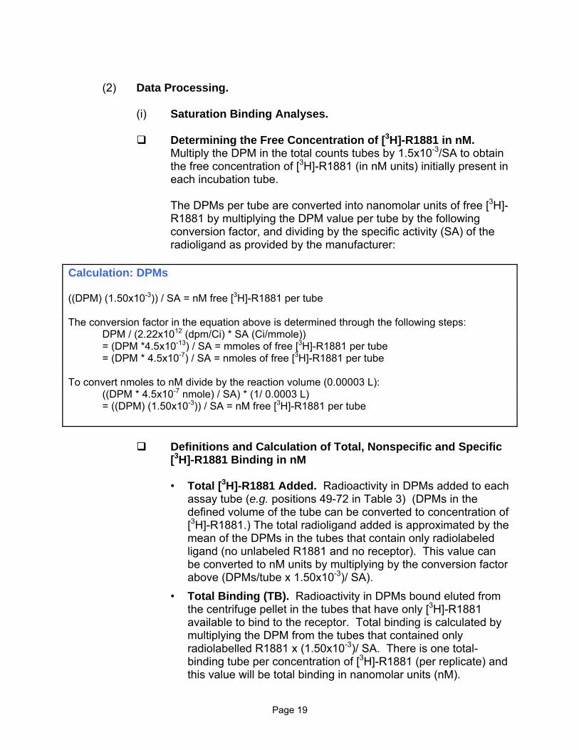
(2) Data Processing.

(i) Saturation Binding Analyses.

Determining the Free Concentration of [3H]-R1881 in nM. Multiply the DPM in the total counts tubes by 1.5x10-3/SA to obtain the free concentration of [3H]-R1881 (in nM units) initially present in each incubation tube.

The DPMs per tube are converted into nanomolar units of free [3H]-R1881 by multiplying the DPM value per tube by the following conversion factor, and dividing by the specific activity (SA) of the radioligand as provided by the manufacturer:

Calculation: DPMs ((DPM) (1.50x10-3)) / SA = nM free [3H]-R1881 per tube The conversion factor in the equation above is determined through the following steps: DPM / (2.22x1012 (dpm/Ci) * SA (Ci/mmole)) = (DPM *4.5x10-13) / SA = mmoles of free [3H]-R1881 per tube = (DPM * 4.5x10-7) / SA = nmoles of free [3H]-R1881 per tube To convert nmoles to nM divide by the reaction volume (0.00003 L): ((DPM * 4.5x10-7 nmole) / SA) * (1/ 0.0003 L) = ((DPM) (1.50x10-3)) / SA = nM free [3H]-R1881 per tube

Definitions and Calculation of Total, Nonspecific and Specific [3H]-R1881 Binding in nM

• Total [3H]-R1881 Added. Radioactivity in DPMs added to each

assay tube (e.g. positions 49-72 in Table 3) (DPMs in the defined volume of the tube can be converted to concentration of [3H]-R1881.) The total radioligand added is approximated by the mean of the DPMs in the tubes that contain only radiolabeled ligand (no unlabeled R1881 and no receptor). This value can be converted to nM units by multiplying by the conversion factor above (DPMs/tube x 1.50x10-3)/ SA).

• Total Binding (TB). Radioactivity in DPMs bound eluted from the centrifuge pellet in the tubes that have only [3H]-R1881 available to bind to the receptor. Total binding is calculated by multiplying the DPM from the tubes that contained only radiolabelled R1881 x (1.50x10-3)/ SA. There is one total-binding tube per concentration of [3H]-R1881 (per replicate) and this value will be total binding in nanomolar units (nM).

Page 19

• Non-specific Binding (NSB). Radioactivity in DPMs bound eluted from the centrifuge pellet in the tubes that contain 100-fold excess of unlabeled over labeled R1881. Nonspecific binding is calculated by multiplying the DPM from the tubes containing radiolabelled R1881 + 100-fold molar excess of radioinert R1881 x (1.50x10-3)/ SA. T here is one NSB tube per concentration of [3H]-R1881 (per replicate), and this value will be nonspecific binding in nM.

• Specific Binding (SB). Total binding minus non-specific binding, in DPMs. Values are calculated during model fitting of total binding and non-specific binding rather than as combinations of the total and non-specific data points gathered. In general specific binding is calculated by subtracting nonspecific binding from total binding using the values determined above (i.e., total binding - nonspecific binding = specific binding) to yield specific binding in nM units.

• BBmax and Ka / Kd. Maximal binding capacity (Bmax) and association/dissociation constants (Ka / Kd) can be estimated using a number of commercially available iterative nonlinear regression analysis programs. Examples of software commonly used for this purpose include LIGAND (Munson and Rodbard, 1980) and GraphPad PRISM (Motulsky, 1995).

Graphical Presentation of the Data

• Saturation Binding. Saturation binding experiments measure

radioligand binding at equilibrium at various concentrations of the radioligand. Correct analysis of these data will determine the maximum receptor number (B max) and the dissociation constant (Kd) of the AR for [3H]-R1881.

Two types of graphical representation are recommended:

1. Saturation curve: Plot Total, Nonspecific, and Specific

binding in dpms on the Y-axis versus the concentration of radioligand in dpms on the X-axis. It is appropriate to use non-linear regression (e.g., BioSoft; McPherson, 1985; Motulsky, 1995) to fit the total binding and non-specific binding data points (not specific binding values, which are calculated not measured), and automatic outlier elimination using the method of Motulsky and Brown (2006) (implemented in Prism 5 software as the ROUT procedure) with a Q value of 1.0. If ligand depletion is a problem, use the method of Swillens (1995). The following model can be used to fit the data:

Page 20

)*(*max XNSKX

XBY

d

++

=

where Y = total binding, NS = non-specific binding, and X = concentration of [3H]-R1881.

Plot each data point (one per replicate for total binding and for non-specific binding, but none for specific binding) as well as the fitted curves for total, specific, and non-specific binding. The specific binding curve is used to visually demonstrate that specific binding is saturated (i.e. reaches a plateau). Determine the Kd and Bmax from this nonlinear regression fit.

2. Scatchard analysis: Plot Specific Binding (Bound) in M on the X-axis versus the ratio of Bound divided by Free radioligand on the Y-axis. This is often referred to as a Scatchard plot. The Scatchard plot is linear, and severe deviations from linearity may indicate that the assay was not performed correctly. The Scatchard plot is not recommended for use in determining the Kd and Bmax values.

(ii) Competitive Binding.

Estimating the IC50. Standard Curve and Test Chemical

Competitive Binding Curves: Plot the data for the standard curve and each test chemical as the percent [3H]-R1881 bound versus the molar concentration. Determine estimates of the IC50s using appropriate non linear curve fitting software such as GraphPad PRISM (GraphPad Software, Inc., San Diego, CA).

The response curve is fitted by weighted least squares nonlinear regression analysis with weights equal to 1/Y. Model fits are carried out using a non-linear regression program such as Prism software (Version 3 or higher). Concentration response trend curves are fitted to the percent of control activity values within each of the repeat tubes at each test chemical concentration. Concentration is expressed on the log scale. In agreement with past convention, common logarithms (i.e., base 10) are used.

The following concentration-response curve is fitted to relate percent of control activity to logarithm of concentration within each run:

Page 21

Y = Bottom + _______________(Top-Bottom)________________ 1+10(Log IC50-X)HillSlope+log[(Top-Bottom)/(50-Bottom)-1]

Where X is the logarithm of the concentration of test substance and Y is the percent of radioligand bound to the receptor. LogIC50 is X at Y=50%. “Top” and “Bottom” refer to the value of Y when there is minimal binding by test chemical, and when there is maximal binding by test chemical, respectively. A concentration-response model is fitted for each test run for each test chemical.

More detailed information on fitting the competitive binding curve and calculating IC50 values is included in Appendix A: How to estimate log(IC50) using curve-fitting software.

Calculation of RBA. Relative Binding Affinity: Calculate the

RBA for each competitor by dividing the IC50 for R1881 by the IC50 of the competitor and expressing as a percent (e.g., RBA for R1881 =100 %).

%RBA = _ (IC50 R1881) X 100 (IC50 Test Substance)

(h) Performance Criteria.

(1) Reasonableness Checks for the Saturation Binding Assay. When evaluating data from AR saturation binding assays, the following factors are recommended for consideration in judging the reasonableness of the results. General considerations are being provided as guidance rather than as specific performance criteria, and include the following:

As increasing concentrations of [3H]-R1881 were used, does the

specific binding curve reach a plateau? For saturation of the AR with the ligand to be obtained, maximum specific binding is required.

If a Scatchard analysis was performed, do the data produce a linear Scatchard plot (a plot of bound/free ligand as a function of specific binding)?

Is the Kd within an acceptable range? The values for Kd in the EPA validation program ranged from 0.685 to 1.57 nM and values within this range are preferred.

Is non-specific binding excessive? The non-specific binding for the assay in the EPA validation program ranged from 8.1-10.0%. The

Page 22

suggested value for non-specific binding is less than 20% of the total binding.

(2) Reasonableness Checks for Competitive Binding Assay. The

competitive binding assay is functioning correctly if all of the following criteria have been met. The criteria apply to each individual run. If a run does not meet all of the performance criteria, a repeat of that run is encouraged. Results for test chemicals in disqualified runs are not recommended for use in classifying the AR binding potential of those chemicals.

(i) Increasing Concentrations of Unlabeled R1881 Displace [3H]-

R1881 from the Receptor in a Manner Consistent with One-site Competitive Binding. Specifically, the curve fitted to the radioinert-R1881 data points using non-linear regression descends from 90–10% over approximately an 81-fold increase in the concentration of radioinert-R1881 (i.e., this portion of the curve will cover approximately 2 log units). A test chemical that binds to the androgen receptor is expected to behave in a similar manner using the one-site competitive binding model. A binding curve that drops dramatically (e.g., from 90-0%) over one order of magnitude is questionable, as is one that is U-shaped (i.e., percent bound is decreasing with increasing concentration of competitor but then begins to increase again). In both cases, something has happened to the dynamics of the binding assay and the reaction is no longer following the law of mass action. When the assay is correctly performed, radioinert R1881 exhibits typical one-site competitive binding behavior. The performance criteria for R1881 reflect this requirement.

(ii) Ligand Depletion is Minimal. Generally ligand depletion is not a

problem in the AR binding assay. However, if it is noted, the recommended ratio of total binding in the absence of competitor to the total amount of [3H]-R1881 added per assay tube is no greater than 10-15%.

(iii) The Parameter Values (top, bottom, and slope) for the

Standard Curve (R1881), and the Concurrent Weak Positive Control (dexamethasone), are Within the Tolerance Bounds Provided. (See Table 5 for the suggested ranges for the parameters.)

(iv) The Solvent Control Substance does not Alter the Sensitivity

or Reliability of the Assay. It is recommended that all test tubes contain equal amounts of solvent.

Page 23

In addition to meeting the criteria for individual runs, examine the consistency across runs for the same chemical. Consistency is encouraged for datasets that can be fit to a curve in the the top plateau level, Hill slope, and placement along the X-axis. Where a bottom is defined, consistent bottom values are recommended.

(3) Limits on Parameters for the Standard, Weak Positive, and Test

Chemical Curves. The following tolerance intervals are provided as guidance by which to judge whether output from the curve fitting model fall within a preferable performance range.

Table 5. Performance Standards.

Chemical Parameter Lower limit Upper Limit Standard Curve Slope -1.2 -0.8 Top (%) 82 114 Bottom (%) -2.0 +2.0 Weak Positive Slope -1.4 -0.6 Top (%) 87 106 Bottom (%) -12 +12

For all test chemicals, it is recommended that the top of the curve fall within 80-115% binding. If a curve starts at a much lower or higher % binding, then a repeat run is encouraged.

(i) Data Interpretation Procedure.

The classification of a chemical as a binder or non-binder is made on the basis of the average results of three runs.

Table 6. Data Interpretation Criteria.

Criteria Classification Average curve across runs crosses 50%* Binder Average lowest portion of curves across runs is between 50% and 75% activity **

Equivocal Data fit 4-parameter nonlinear regression model

Average lowest portion of curves across runs is greater than 75% activity**

Data do not fit the model ---

Non-Binder

*Ordinarily, a binding curve will fall from 90% to 10% over 2 log units with a slope near -1. If the curve falls outside the range for the weak positive control (-0.6 to -1.4), classify the run as equivocal. Unusually steep curves may be a sign that the protein is being denatured or that solubility problems are being encountered. **If the test compound is not soluble above 10-6 M and the binding curve does not cross 50%, the chemical is judged to be un-testable. If the curve is steeper than -2.0 the result is considered to be equivocal. (j) Data Reporting.

(1) Saturation Binding Assay. For each run, provide at least the following. Be sure to include a run identifier on each product. When preparing

Page 24

graphs, use the same axis length and range on all comparable graphs to facilitate comparisons across runs.

The following information, as well as any additional relevant information, is requested in the test report:

Radioactive Ligand ([3H]-R1881).

- Name, including number and position of tritium atom(s). - Supplier, catalogue number, and batch number. - Specific Activity (SA) and date for which that SA was certified by

supplier. - Concentration as received from supplier (Ci/mmol). - Concentrations tested (nM). If dilutions were prepared using a

scheme different from Table 3 Saturation Assay Tube Layout, provide an analogous table showing how dilutions were made.

Radioinert Ligand (R1881).

- Supplier, batch number, catalog number, CAS number, and purity.

- Concentrations added to NSB tubes (nM). If dilutions were prepared using a scheme different from Table 3 Saturation Assay Tube Layout, provide an analogous table showing how dilutions were made.

Androgen Receptor.

- Source of rat prostate cytosol. Please identify the source of the animals used (i.e., the supplier), including information on the strain and age (at necropsy) of rats from which prostate glands were taken, and time between castration and removal of the prostate. For each batch of cytosol, report the time of kill for each animal whose prostate was used in the batch.

- Isolation procedure. - Protein concentration of AR preparation. Provide details of the

protein determination method, including the manufacturer of the protein assay kit, data from the calibration curves, and data from the protein determination assay.

- Method and conditions of transport and storage of AR, if applicable.

Test Conditions. - Protein concentration used. - Total volume per assay tube during incubation with receptor.

Page 25

- Incubation time and temperature. - Notes on any abnormalities during separation of free

radiolabeled R1881. - Notes on any problems in analysis of bound radiolabeled

R1881. - Statistical methods used when estimating Kd and Bmax.

Test Results. For each run, provide at least the following. Be sure

to include a run identifier on each product. When preparing graphs, try to use the same axis length and range on all comparable graphs to facilitate evaluation across runs. Insert results (e.g., the dpm counts for each tube) into a data worksheet, adjusted as necessary to accommodate the actual concentrations, volumes, etc. used in the assay. Report data in electronic format (spreadsheet or comma-separate values), being sure to provide all formatting information that is necessary to read the data. The Agency intends to provide a suggested template on the Agency’s Web site (Ref. 1). One worksheet per run is requested.

- Date of run, number of days since SA certification date, and

adjusted SA on day of run. - A graph of total, specific, and non-specific binding across the

range of concentrations tested. Plot each data point (one per replicate for total binding and for non-specific binding, but none for specific binding) as well as the fitted curves for total, specific, and non-specific binding. Use a method that fits total binding and non-specific binding simultaneously (i.e., shares the non-specific binding parameter). Account for ligand depletion using the method of Swillens (1995), and exclude outliers using the method of Motulsky and Brown (2006) using a Q-value of 1.0.

- A graph of measured concentrations in the total [3H]-R1881 tubes.

- Scatchard plot, using nM for the units of the specific bound (X) axis. Show each data point. If ligand depletion is noted, then instead of showing the best-fit line through the data points, plot the line based on the Swillens correction for ligand depletion (i.e., the line based on the Bmax and Kd estimated from the data when the Swillens correction is used). Include the values for Kd (in nM) and Bmax (in both nM and fmol/100 μg protein), estimated when ligand depletion is accounted for, on this graph.

- Raw data (decays per minute) for each tube, as well as the components of each tube (volumes and concentrations).

- Provide the following information summarizing the information from all of the runs for each batch of cytosol:

Page 26

A graph showing total, non-specific, and specific binding for all runs done on that batch. Be sure to differentiate runs by color and date.

A table of Kds and Bmaxs for all runs on that batch.

Conclusion. - Give the estimated Kd and standard error of the mean of the

radioligand ([3H]-R1881). - Give the estimated Bmax and standard error of the mean across

all runs for each batch of cytosol prepared. - Briefly note any reasons why confidence in these numbers is

high or low.

(2) Competitive Binding Assay

The following information, and any additional relevant information, is requested in the test report:

Test Substance. - Name, chemical structure, and CAS RN (Chemical Abstract

Service Registry Number, CAS#), if known. - Physical nature (solid or liquid), and purity, if known. - Physicochemical properties relevant to the study (e.g., solubility,

stability, volatility).

Solvent/Vehicle. - Justification for choice of solvent/vehicle. - Concentration of solvent (as percent of total volume) at each

concentration of R1881, weak positive, negative control, solvent control, and test chemical.

Reference Androgen. (e.g., radioinert R1881)

- Supplier, batch, and catalog number. - CAS number. - Purity.

Androgen Receptor. - Source of rat prostate cytosol. Please identify the source of the

animals used (i.e., the supplier), including strain and age of rats from which ventral prostates were taken, and timing between

Page 27

castration and removal of the prostate. For each batch of cytosol, report the time of kill for each animal whose prostate was used in the batch.

- Isolation procedure. - Protein concentration of AR preparation. Provide details of the

protein determination method, including the manufacturer of the protein assay kit, data from the calibration curves, and data from the protein determination assay.

- Method and conditions of transport and storage of AR, if applicable.

Test Conditions.

- Kd of R1881. Report the Kd obtained from the Saturation Binding Assay for each batch of cytosol used.

- Concentration range and spacing of the reference and weak positive.

- Concentration range and spacing of solvent controls. - Concentration range and spacing of test substance, with

justification if deviating from recommended range and spacing. - Dilution schemes used for preparing the concentrations of

R1881, weak positive, and test chemical. (If the schemes used in the protocol were used without modification, state that.)

- Composition of buffer(s) used. - Incubation time and temperature. - Notes on any abnormalities during separation of free

radiolabeled R1881. - Notes on any problems in analysis of bound R1881 or the weak

positive. - Notes on reasons for repeating a run, if a repeat was necessary. - Methods used to determine log(IC50) values (software used,

formulas, etc.). - Statistical methods used, if any.

Results.

- Insert results (e.g., the dpm counts for each tube) into a data worksheet, adjusted as necessary to accommodate the actual concentrations, volumes, etc. used in the assay. Report data in electronic format (spreadsheet or comma-separate values), being sure to provide all formatting information that is necessary to read the data. The Agency intends to provide a suggested template on the Agency’s Web site (Ref. 1). One worksheet per run is requested.

Page 28

- Date of run, number of days since Specific Activity (SA) certification date, and adjusted SA on date of run.

- Extent of precipitation of test substance. - Compare the solvent control responses at the beginning and

end of the assay to check for drift in the assay. - % Binding data for each replicate at each dose level for all

substances. - Plot the data points and the unconstrained curve fitted to the Hill

equation for each run of each chemical, separately (that is, one test chemical run per graph). Also plot the data points and curves for the reference chemical and weak positive control from that test chemical’s run on the same graph as the test chemical.

- Plot the curves showing the mean +/- SEM for all for all runs for each chemical on separate graphs. Do not plot the inert R1881, or weak positive information on this graph but plot them separately.

- Log(IC50) values for R1881, the positive control, and the test substance. Show mean and SE for each compound.

- Calculated Relative Binding Affinity values for the positive control and the test substance, relative to RBA of R1881 = 1.

- Document all protocol deviations or problems encountered and included in the final report. Use this information to improve subsequent runs.

- A summary sheet of the performance criteria measures for each run.

Conclusion.

- Classification of test substance with regard to interaction with the androgen receptor (binder, equivocal, non-binder, or untestable (does not reach 50% reduction in binding and is not soluble above 10-6 M).

- If the test substance is a binder, estimate the RBA by averaging the RBAs obtained across the acceptable runs. Report the range of RBAs also.

(3) Replicate Studies. Generally, replicate studies are not mandated for

screening assays. However, in situations where questionable data are obtained (i.e., the IC50 value is not well defined), replicate tests to clarify the results of the primary test would be prudent.

(k) References. 1. EPA. OPPTS Harmonized Test Guidelines. Available on-line at:

http://www.epa.gov/oppts (select “Test Methods & Guidelines” on the left side

Page 29

http://www.epa.gov/oppts

navigation menu). You may also access the guidelines in http://www.regulations.gov grouped by Series under Docket ID #s: EPA-HQ-OPPT-2009-0150 through EPA-HQ-OPPT-2009-0159, and EPA-HQ-OPPT-2009-0576.

2. ICCVAM (2006). Addendum to ICCVAM Evaluation of In Vitro Test Methods for

Detecting Potential Endocrine Disruptors: Estrogen Receptor and Androgen Receptor Binding and Transcriptional Activation Assays. NIH Publication No: 03-4503.

3. Motulsky, H.J. (1995). Analyzing data with GraphPad Prism, GraphPad Software

Inc., San Diego CA, http://www.graphpad.com. 4. Motulsky, H.J. and Brown, R.E. (2006). Detecting Outliers When Fitting Data with

Nonlinear Regression – A New Method Based on Robust Nonlinear Regression and the False Discovery Rate. BMC Bioinformatics 7:123-142.

5. Munson, P.J., and Rodbard, D. (1980). Anal Biochem. 107: 220-239. 6. Nonneman, D.J., Ganjam, V.K., Welshons, W.V., and Vom Saal, F.S. (1992). Biol

Reprod 47: 723-729. 7. Owens, W., Zeiger, E., Walker, M., Ashby. J., Onyon, L., and Gray, Jr., L.E.

(2006). The OECD programme to validate the rat Hershberger bioassay to screen compounds for in vivo androgen and antiandrogen responses. Phase 1: Use of a potent agonist and a potent antagonist to test the standardized protocol. Env. Health Persp. 114:1265-1269. See, section II, The dissection guidance provided to the laboratories: http://www.ehponline.org/docs/2006/8751/suppl.pdf.

8. Prins, G. (1989). Differential regulation of androgen receptors in the separate rat

prostate lobes: androgen independent expression in the lateral lobe. J Steroid Biochem 33(3):319-326.

9. Segel, I.H. (1975). Enzyme Kinetics: Behavior and Analysis of Rapid Equilibrium

and Steady-State Enzyme Systems; First edition. New York: John Wiley & Sons, Inc.

10. Swillens, S. (1995). Interpretation of binding curves obtained with high receptor

concentrations: practical aid for computer analysis. Molec. Pharmacol. 47(6):1197-1203.

11. Tekpetey, F.R., and Amann, R.P. (1988). Biol Reprod 38: 1051-1060. 12. Wilson, V.S., Lambright, C.S., Ostby, J., and Gray, Jr., L.E. (2002). In vitro and in

vivo effects of 17β-trenbolone: A feedlot effluent contaminant. Toxicol Sci 70(2): 202-11.

Page 30

http://www.regulations.gov/

http://www.graphpad.com/

http://www.ehponline.org/docs/2006/8751/suppl.pdf

A - 1

Appendix A: How to Estimate Log(IC50) Using Curve Fitting Software A few words about terms: IC50 and EC50 Please note that the terms IC50 (inhibitory concentration, 50%) and EC50 (effective concentration, 50%) refer to two different concepts. The IC50 is the concentration of test substance at which 50% of the radioligand is displaced from the androgen receptor. The EC50 is the concentration of test substance at which binding of the radioligand is halfway between the top plateau and the bottom plateau of the curve defined (as for determination of the IC50) by fitting the Hill equation to the data specific to that test substance and run. Where an IC50 exists, it may or may not be equal to the EC50. (An IC50 may not always exist – the fitted curve may not cross the 50% binding level – but the EC50 will always exist provided the Hill equation can be fit to the data.) The IC50 provides the more consistent basis for evaluating interaction of the test chemical with the androgen receptor and thus is preferred to the EC50 for purposes of the Endocrine Disruptor Screening Program. Because the Hill equation describes the fraction of receptor bound by ligand as a function of the logarithm of the ligand concentration, we will more often refer to log(IC50) and log(EC50) than to the untransformed values. In these terms, when X is the concentration of test substance and Y is the % of radioligand bound to the androgen receptor,

• log(IC50) is the log10(X) at which Y is 50%. • log(EC50) is the log10(X) at which Y is (top + bottom)/2.

Methods for calculating log(IC50) Method 1: Fit a curve to the data using a Hill equation formula which incorporates log(IC50) as a parameter to be estimated. Method 2: Fit a curve to the data using a form of the Hill equation in which log(IC50) is not a parameter. After the curve is fit, the log(IC50) is interpolated. Generally method 1 is the most appropriate and most utilized method but a description of method 2 is included here for cases where the graphing software is unable to fit a curve and provide an IC50 value, even when the data includes points below the y=50 value. Method 1: Fitting data to an IC50 formula In this method, data are fit to a formula that directly estimates log(IC50). The formula used for curve-fitting is Y=Bottom + (Top-Bottom)/(1+10^((LogIC50-X)*HillSlope+log((Top-Bottom)/(50-Bottom)-1))) where X is the logarithm of the concentration of test substance and Y is the percent of radioligand bound to the receptor. LogIC50 is X at Y=50%. “Top” and “Bottom” refer to the value of Y when there is minimal binding by test chemical, and when there is

A - 2

maximal binding by test chemical, respectively. This formula may need to be entered manually into the curve-fitting software; it is not, for example, available as a standard formula in GraphPad Prism at the time of this writing. Method 2: Fitting data to an EC50 formula and interpolating an IC50, where possible Sometimes when using Method 1 software will issue an error message such as “Floating point error,” “Bad initial values,” or “Does not converge.” This can happen either when:

• there is no log(IC50) that can be estimated (e.g., the bottom is greater than 50%); or

• the software cannot handle a huge number encountered in the estimation process even if the log(IC50) exists. (That is, the underlying curve, if the software could calculate it, crosses the horizontal line corresponding to Y=50% but the software was unable to define that curve because of computational difficulties.)

In the latter case, adjusting initial values used by the curve fitting program may result in a successful fit if the defaults do not. Also, statistical software packages such as Stata or SAS often are able to fit a model to a data set that smaller packages such as GraphPad Prism are unable to fit. Another approach that may be successful is to fit a formula that estimates the log(EC50), then calculate the log(IC50) from the point at which the fitted curve crosses the 50% line. The formula for estimating log(EC50) is

Y = Bottom + (Top-Bottom)/(1+10^((LogEC50-X)*HillSlope)) By solving the following equation for X, we can get log(IC50) from the log(EC50) results (as long as the curve crosses Y=50%):

50 = Bottom + (Top-Bottom)/(1+10^((LogEC50-X)*HillSlope)) Forcing this interpolation may not be straightforward. In GraphPad Prism software, for example, it is necessary to include a fake data point that has a “missing” X value in the data set. By including this fake data point and checking the “Unknown from standard curve” box, we can make Prism report the X value corresponding to Y = 50 % (which is the definition of log(IC50) in the “Interpolated X mean values” sheet in the “Results” folder. This method of using Prism’s built-in method for fitting the unconstrained Hill equation first and then interpolating the log(IC50) has the advantage that it provides the top, bottom, slope, and log(EC50) values when the log(IC50) does not exist or the log(IC50) model fit fails. A disadvantage is that Prism does not report the standard error of the log(IC50) through this method, which it will do when an explicit log(IC50) model is fit.

united states epa 640-c-09-003 and toxic substances ...€¦ · endocrine disruptor screening...

Documents