Lectures on Landau Theory

of Phase Transitions

University of Leeds, Department of Physics and Astronomy

Peter D Olmsted

February 2, 2000

Contents

1 Goals of these Lectures 1

2 Phase Transitions 2

2.1 Examples . . . . . . . . . . . . . . . . . . . . . . . . . . . . . . . . . . . . . 2

2.2 Statistical Mechanics and Phase Transitions . . . . . . . . . . . . . . . . . . 3

3 Landau Theory: Fundamentals 5

3.1 The Recipe . . . . . . . . . . . . . . . . . . . . . . . . . . . . . . . . . . . . 5

3.2 Relation to Statistical Mechanics . . . . . . . . . . . . . . . . . . . . . . . . 6

4 Examples 7

4.1 Ising Magnet . . . . . . . . . . . . . . . . . . . . . . . . . . . . . . . . . . . 8

4.2 Heisenberg Ferromagnet . . . . . . . . . . . . . . . . . . . . . . . . . . . . . 9

4.3 Nematic Liquid Crystals . . . . . . . . . . . . . . . . . . . . . . . . . . . . . 10

4.4 Crystal Systems . . . . . . . . . . . . . . . . . . . . . . . . . . . . . . . . . . 14

4.4.1 Lamellar Systems . . . . . . . . . . . . . . . . . . . . . . . . . . . . . 14

4.4.2 Two and Three Dimensional Crystals . . . . . . . . . . . . . . . . . . 15

i

5 Smectic Liquid Crystals 18

5.1 Mean Field Theory of the Nematic-Smectic{A transition . . . . . . . . . . . 18

5.2 Free Energy and Superconducting Analogy . . . . . . . . . . . . . . . . . . . 19

5.3 Fluctuations and the Halperin-Lubensky-Ma E�ect. . . . . . . . . . . . . . . 21

5.4 Layered liquids and the Brazovskii e�ect . . . . . . . . . . . . . . . . . . . . 23

ii

1. Goals of these Lectures Lectures on Landau Theory

1 Goals of these Lectures

Phase transitions are ubiquitous in nature. Examples include a magnets, liquid crystals,

superconductors, crystals, amorphous equilibrium solids, and liquid condensation. These

transitions occur between equilibrium states as functions of temperature, pressure, magnetic

�eld, etc.; and de�ne the nature of the matter we deal with on a day to day basis. Under-

standing how to predict and describe both the existence of these transitions, as well as their

character and consequences for everyday phenemena, is one of the more important roles of

statistical and condensed matter physics.

In this set of Lectures I propose to outline one of the basic theoretical tools for describing

phase transitions, the Landau Theory of Phase Transitions. This was developed by

Landau in the 1940's, originally to describe superconductivity. The procedure is general,

and is one of the most useful tools in condensed matter physics. Not only can we use

Landau Theory to describe and understand the nature of phase transitions among ordered

(and disordered) states, but we can use it as a starting point for understanding the behavior

of ordered states. These lectures are designed to establish the following broad brush strokes:

1. Very few phase transitions can be calculated exactly: nonetheless, there is still much

that can be understood without having to solve the entire problem. These kinds of

questions (order of phase transitions, hydrodynamics and elasticity, uctuations) are

the domain of Landau theory.

2. I will present (some of) the problems of phase transitions, and introduce Landau Theory

as a way of understanding the behavior (but not the existence) of phase transitions.

3. We will explore, through examples, the profound implications of symmetry for the

nature of ordered states and their associated transitions.

4. We will see how to use the nature of the order parameter to understand deformations

in a broken symmetry state: this often goes by the name of generalized elasticity,

and incorporates elasticity of solids, Frank elasticity in nematic liquid crystals, the

deformation energy of smectic liquid crystals and membrane systems, sound waves in

uids, etc.

5. Landau theory is a mean �eld theory, in the sense that the system is assumed to be

adequately described by a single macroscopic state.

6. We will use Landau free energy functionals to calculate observable quantities such as

structure factors; identify the breakdown of Landau theory due to uctuations.

7. We will examine some interesting paradigms whereby the qualitative nature of phase

transitions, such as the order of the phase transition, is altered by uctuation e�ects

and the coupling of di�erent degrees of freedom.

Along the way we will learn how to follow our noses and construct proper free energy

functionals on symmetry grounds; pick up some calculational tools; and examine some fun-

damental ideas in statistical mechanics.

1

2. Phase Transitions Lectures on Landau Theory

2 Phase Transitions

A phase transition occurs when the equilibrium state of a system changes qualitatively as

a function of externally imposed constraints. These constraints could be temperature, pres-

sure, magnetic �eld, concentration, degree of crosslinking, or any number of other physical

quantities. In the following I only consider a transition as a function of temperature, but

note that the idea is, of course, more general than that (physicists strive to be as general as

possible!). In any of these transitions there is some quantity that can be observed to change

qualitatively as a function of temperature. In many cases more than one quantity can be

observed, but it is quite obvious that something is happening. This quantity will be taken

later to be the order parameter of the phase transition.

2.1 Examples

1. Crystals: In a transition to a crystalline solid a disordered liquid with non apparent

structure undergoes a transition to a structure with long range periodic order, usually

in three dimensions. This is most easily parametrized by the mass density, �(r):

�(r) = ��+Xq2G

��(q)e�iq�r + c:c

�; (2.1)

where �� is the mean density and fGg is theset of reciprocal lattice vectors that char-

acterize the crystal structure. The Fourier

modes refer to density modulations with

wavenumber q = 2�=�, with wavelength

�. The complex conjugate is added to re-

tain a real number for the mass density.

Upon cooling a liquid into a crystal the

object that distinguishes the crystal from

the liquid is the set of wavevectors f�(G)g,which appear as Bragg peaks in a scat-

tering experiment. Usually these Fourier

modes grow discontinuously from zero, in

what is called a �rst order phase tran-

sition:

Tc

Temperature

orde

r pa

ram

eter

First Order Phase Transition(Nematic LC, 2D/3D crystals, etc)

2. Nematic Liquid Crystals: The isotropic-nematic transition occurs in melts (or

solutions) of rigid rod-like molecules. At high temperatures (or dilute concentrations)

the rods are isotropically distributed, and upon cooling an orientational interaction

which is a combination of enthalpic and excluded volume e�ects encourages the rods

to spontaneously align along a particular direction, denoted the director, bn. A scalar

measure of the order is the anisotropy of the distribution of rods,

hP2(cos �)i = hcos2 � � 13i; (2.2)

where the average h�i is taken over the equilibrium distribution for all rods in the

system, and � is the angle with respect to some �xed direction. Like 2D crystallization,

2

2.2 Statistical Mechanics and Phase Transitions Lectures on Landau Theory

the isotropic-nematic is a �rst order transition, with a discontinuity in hP2(cos �)i at thetransition temperature TIN . Since \up" and \down" are the same for such a system (in

liquid crystals the rodlike molecules are typically symmetric under re ection through

the long axis), the order parameter is symmetric under cos � ! � cos �.

3. Magnets: In a ferromagnet an assembly

of magnetic spins undergoes a spontaneous

transition from a disordered phase with no

net magnetization to a phase with a non-

zero magnetization. The order parameter

is thus the magnetization,

M =1

N

Xi

hSii; (2.3)

where the average is an equilibrium aver-

age over all spins Si in the system. Un-

like the nematic liquid crystal, the ferro-

magnetic phase transition is a continuous

phase transition, in which the magne-

tization grows smoothly from zero below

a critical temperature Tc (often called the

Curie Temperature, after its discoverer).

Tc

Temperature

orde

r pa

ram

eter

Continuous Phase Transition (Magnet, superconductor, 1D crystal, ...)

4. One Dimensional (layered) Crystals: In a one dimensional crystal, or a layered

system, a one-dimensional modulation develops spontaneously below the critical tem-

perature. Examples include block-copolymers, which can phase separate into layers of

A and B material, to relieve chemical incompatibility but maintain the connectivity

constraint; helical magnets which develop a pitch as the spin twists; cholesteric phases

which develop a twisted nematic conformation; and smectic phases in thermotropic

liquid crystals and lyotropic surfactant solutions. In this case the order parameter is

the Fourier mode of the relevant degree of freedom:

(r) = � + (q)e�iq�r + c:c: (2.4)

This transition is predicted by Landau (mean �eld) theory to be continuous, but it is

believed to be �rst order in physical situations, due to uctuation e�ects. Hopefully

we will get this far!

5. Phase Separation: Finally, one of the most common phase transitions from every

day life is phase separation, which makes it necessary to shake the salad dressing. In

this case the order parameter is the deviation of the local composition from the mean

value. Usually this is a �rst order phase transition, but if the concentration is just

right the system can be taken through a critical point, or continuous phase transition.

This system is equivalent to liquid-liquid or liquid-gas phase separation, in which case

the order parameter is a density di�erence instead of a composition di�erence.

2.2 Statistical Mechanics and Phase Transitions

One of the uses of statistical mechanics (aside from helping us to understand nature) is to

calculate fundamental properties of matter, including phase transitions. In principle, this

3

2.2 Statistical Mechanics and Phase Transitions Lectures on Landau Theory

is a remarkably simple task, thanks to Boltzmann. All of the statistical information of a

system is encoded in the Partition Function, Z:

Z =X�

e�H[�]=kBT ; (2.5)

where � refers to all the microstates of the system (e.g. all possible con�gurations spins in

a magnet) and H[�] is the Hamiltonian (energy). Boltzmann proved that the (Helmholtz)

free energy is given by

F = �kBT lnZ: (2.6)

If we can calculate the free energy F we can then calculate all desired thermodynamic

quantities by appropriate derivatives.� Unfortunately, the free energy can only be evaluated

for a few systems, notably the Ising Model (spins which can point up or down, and interact

with each other by a very simple interaction, H = �JPij SiSj). More often than not we

are faced with an impossibly diÆcult calculation.

In the case of phase transitions, perhaps we can get away with a less rigorous calculation.

A clue is the very nature of a phase transition: at a phase transition a system undergoes a

qualitative change, and develops some order where there was none before. Hence the system

does not vary smoothly as a function of (for example) temperature. This means that the

free energy F (T ) is, mathematically, a non-analytic function of temperature. This is of

fundamental importance in the theory of phase transitions, and forms the starting point of

rigorous studies. A non-analytic function is one for which some derivatives are unde�ned

at certain points, or singularities. Phase transitions are points (in the parameter space of

�eld variables such as temperature, pressure, magnetic �eld) or sets of points which are

singularities in the free energy. The free energy, and hence the behavior of a thermodynamic

system, behaves non-smoothly as it is taken through a phase transition.

It's interesting to try and understand how to get non-analytic behavior out of a sum of

exponentials, each of which is separately analytic at any �nite temperature:

F = �kBT ln

"X�

e�H[�]=kBT

#: (2.9)

The existence of singularities in F is a direct result of the thermodynamic limit, that is, the

presence of an essentially in�nite number of degrees of freedom in a thermodynamic system.

�For example, the magnetization can be determined by

M = �

�@F

@h

�h=0

; (2.7)

where an additional symmetry-breaking �eld has been added to the system Hamiltonian. For any system,

it's only a matter of cleverness to determine the extra �eld to add to \extract" the desired order parameter

by a suitable derivative. In this case the �eld enters as

H[S]! H[S]� hXi

Si: (2.8)

4

3. Landau Theory: Fundamentals Lectures on Landau Theory

Possible singularities we can imagine in F are discontinuities in the �rst derivative, @F=@T ,

or in higher order derivatives @2F=@T 2; @

3F=@T

3; : : : . These two cases de�ne, respectively,

�rst order or continuous (often termed \second order") phase transitions.

TC

Temperature T

Fre

e en

erg

y F

First Order Phase Transition

TC

Temperature T

Continuous Phase Transition

From the theory of analytic functions we are familiar with the fact that a surprising

amount of information is contained in singularities: witness the Cauchy Integral Theorem.

So, if we can somehow come to grips with a singularity in the free energy, even in just a

qualitative way, then perhaps some progress can be made in understanding the physics of

phase transitions. This is the goal of Landau Theory.

3 Landau Theory: Fundamentals

3.1 The Recipe

Landau made a series of assumptions to approximate the free energy of a system, in such a

way that it exhibits the non-analyticity of a phase transition and turns out to capture much

of the physics. There are essentially four steps in this procedure: we will visit these steps

�rst, and then explore them again in terms of the partition function.

1. De�ne an order parameter : For a given system an order parameter must be con-

structed. This is a quantity which is zero in the disordered phase and non-zero in the

ordered phase. Examples include the magnetization in a ferromagnet, the amplitudes

of the Fourier modes in a crystal, and the degree of orientation of a nematic liquid

crystal.

2. Assume a free energy functional: Assume the free energy is determined by minimizing

the following functional

~F = F0(T ) + FL(T; ); (3.1)

5

3.2 Relation to Statistical Mechanics Lectures on Landau Theory

where F0 is an analytic (smooth) function of temperature, and FL(T; ) contains all

the information about dependence on the order parameter .

3. Construction of FL( ): The Landau Functional is assumed to be an analytic (typically

polynomial expansion) function of that obeys all possible symmetries associated with

; this typically includes translational and rotational invariance, and other \internal"

degrees of dicatated by the nature of the order parameter. This is the most important

part of the theory, wherein most of the physics lies.

4. Temperature Dependence: It is assumed that all the non-trivial temperature depen-

dence resides in the lowest order term in the expansion of FL(T; ), typically of the

form

FL[T; ] =

ZdV

�12a0(T � T�)

2 + : : :�

(3.2)

Since FL is constructed as an expansion, there will be other unknown constants. In

a physical system these constants have temperature dependence, but if these depen-

dences are smooth then they have negligible e�ect near the phase transition. This is

rigorous for a continuous phase transition, and an approximation for a �rst order phase

transition.

Upon constructing the Landau functional, and minimizing it over as a function of tem-

perature, the nature of the phase transition may be determined. The system at this level is

speci�ed as having a uniform, or mean, state; hence Landau theory is really a mean �eld the-

ory. However, the resulting approximate free energy is a natural starting point for examining

uctuation e�ects.

3.2 Relation to Statistical Mechanics

To understand what's going on, let's reexamine statistical mechanics. The free energy is

given by

e�F=kBT =

X�

e�H[�]=kBT : (3.3)

Landau's assumption is that we can replace the entire partition function by the following,

e�F=kBT ' e

�F0=kBT

ZD e�FL[T; ]=kBT ; (3.4)

where the integralR D is a functional integral over all degrees of freedom associated with

, instead of an integral over all microstates. For example, if is the mean magnetization,

a given value for the magnetization can be determined by many di�erent microstates. It is

assumed that all of this information is contained in FL. This is a non-trivial assumption which

can nonetheless be proven for certain systems. The conversion of the degree of freedom from

� to is known as coarse-graining, and is at the heart of the relationship between statistical

mechanics and thermodynamics. The next step is to minimize FL[T; ], giving:

e�F=kBT ' e

�F0=kBT e�minf g FL[T; ]=kBT : (3.5)

6

4. Examples Lectures on Landau Theory

This is tantamount to performing a saddle point approximation to the function integral in

Eq. (3.4).

Here's a more formal rationalization:

e�F=kBT =

X�

e�H[�]=kBT exact Partition Function (3.6a)

=X�

ZD Æ[ � h�i]e�H[�]=kBT introduce as an average over � (3.6b)

=

ZD

X�

Æ[ � h�i]e�H[�]=kBT interchange limits (3.6c)

'ZD g( )e�H[ ]=kBT

� g( ) represents the degeneracy of (number of microstates)

� H[�] ! H[ ] is generally incor-

rect, but illustrates the idea.

(3.6d)

=

ZD e�[H[ ]�kBT ln g( )]=kBT (3.6e)

) F ' min

[H[ ]� kBT ln g( )] : saddle point approximation (3.6f)

Now, the free energy of a system is given by

F = E � TS: (3.7)

Hence ln g( ) is essentially the entropy of the system. To rationalize the assumed form of

the temperature dependence of FL[T; ], we write:

F

Volume' E0 �E�

2| {z }attraction

+ : : :� T [S0 �a 2 + : : :| {z }reduction due to ordering

] (3.8a)

= F0 + a(T � E�a) 2 + : : : (3.8b)

We assume there is some \attraction" neccessary to induce order in the system, but this oc-

curs at the expense of reducing the entropy; this, in principle, is contained in the degeneracy

g( ). The competition of these e�ects leads to a phase transition.

In a physical system, the steps between Eq. (3.6c) and Eq. (3.6d) is exceedingly diÆcult,

since the relationship between and � is often not simple, and usually a di�erent functional

form than the appearance of � in the original HamiltonianH[�]. Hence this procedure should

be considered a cartoon; in reality, H[ ] and g[ ] are inextricably and inseparably bound

into FL[ ].y

4 Examples

To make this discussion concrete and useful we must examine some physical systems. We

will do this in order of complexity, and gradually introduce important concepts and gener-

alizations as they appear.

yIn the case of polymer blends, where the Hamiltonian is given by H = �P

�;� �� V�� �� , where ��denote the mean fractions of species � = A;B;C; : : : in the blend and V�� is a matrix of Flory interaction

parameters, the reduction above is essentially correct! This is the RPA (Random Phase Approximation).

7

4.1 Ising Magnet Lectures on Landau Theory

4.1 Ising Magnet

Order Parameter|The Ising Model consists of spins which can only point up or down. At

high temperatures the spins are disordered, and at low temperatures the spins spontaneously

choose whether to point up or down. The order parameter is the mean value of the spins,

M = hSiii+� (4.1)

where the average is within a region � about a given spin. � is the coarse graining length. To

describe local ordering � should be much larger than a lattice spacing a, and to adequately

describe spatial uctuations (later), � should be much smaller than the system size. Since

there are generally 107 orders of magnitude to deal with in a particular system, this separation

of length scales isn't a problem. For most calculations we don't need to specify the value of �,

but it becomes important when we consider non-uniform terms (later) or the renormalization

group (much later!).

Symmetries|The only symmetry which is relevant for M is that up and down are identical

states, related by a rotation of the sample by �. Since we assume the system is rotationally

invariant (for example, it isn't in a magnetic �eld), the free energy in the absence of a

�eld should be invariant under M ! �M . Note that this does not mean that the spins

themselves, or indeed the order parameter, is the same under a ip. This is an important

distinction.

Free Energy|The free energy consistent with this symmetry is

fL � FL

Volume= 1

2a(T � Tc)M

2 + 14cM

4 + : : : (4.2)

Higher order terms M2n are possible, but

we will see that they are not necessary to de-

scribe the transition. As a function of tem-

perature, this free energy has minima at

M =

(0 (T > Tc)

�q

a(Tc�T )

c(T < Tc)

(4.3)

for temperatures T < Tc. This is a con-

tinuous transition, since the magnetization

grows smoothly from zero. We shall see that

this is a feature of all free energies which, by

symmetry, have only even powers of the order

parameter.

0

Order Parameter M

Fre

e E

ner

gy

f L

T>Tc

T<Tc

Thermodynamics|Upon minimizing the free energy, the free energy as a function of tem-

perature is now:

F =

8<:F0(T ) (T > Tc)

F0(T )� V12

ajTc � T j2c

(T < Tc)(4.4)

8

4.2 Heisenberg Ferromagnet Lectures on Landau Theory

(V is the volume). Hence, we see that @F=@T vanishes at the critical point, while the second

derivative has a discontinuity:

@2F

@T 2

����T+c

� @2F

@T 2

����T�c

=a

cV: (4.5)

Hence this is a second order phase transition. This is related to the heat capacity:

CV = T

�@S

@T

�V

= �T @2F

@T 2

����V

: (4.6)

Thus, for the magnet there is a discontinuity (a step decrease) in the heat capacity given by

�CV = �V Ta=c.The Landau free energy has two free parameters, a and c. In principle, these can be

determined by comparison with experiment from the shape of M(T ) and the heat capacity

jump.

4.2 Heisenberg Ferromagnet

Order Parameter|In the Heisenberg ferromagnet (in, say, 3D), the spin can point anywhere

in space. Hence the magnetization is a vector, de�ned in the same was as for the Ising Model:

M = hSiii+� (4.7)

Symmetries|In the magnetic state the system spontaneously chooses a direction in which

to point. In isolation this direction is entirely arbitrary. Hence, the system is rotationally

symmetric with respect to any angle of rotation. Any free energy must be invariant under

M �! R �M; (4.8)

where R is a rotation matrix. If M is the only order parameter in the problem, and space is

isotropic, then any free energy must only depend on the invariant M �M. Under a rotation

this invariant transforms as

M �M!M � RT � R �M =M � I �M =M �M; (4.9a)

where we used the fact that RT � R is the identity matrix I, for any proper rotation.

Free Energy|The free energy consistent with this symmetry is

fL � FL

V= 1

2a(T � Tc)M �M+ 1

4c (M �M)

2+ : : : (4.10)

Odd order terms are not allowed by symmetry. Hence, like the Ising Magnet, the Heisenberg

Magnet has a second order transition. The primary di�erence between the two systems

is that, while the Ising magnet breaks up-down symmetry, the Heisenberg magnet breaks

rotational symmetry: M can point anywhere in space. The free energy surface is often

called the \wine bottle" or \Mexican hat" potential. Below the Curie temperature Tc the

system rolls to the bottom of the wine bottle.

9

4.3 Nematic Liquid Crystals Lectures on Landau Theory

Mexican Hat Potential

Once the system has broken symmetry, the further behavior at a given temperature

(under, say, the action of a small perturbing �eld) is much di�erent than that of the Ising

magnet. While the Ising magnet can change only its magnitude, the Heisenberg magnet

can change both magnitude and direction. From the shape of the potential we can see

that changes in magnitude run up the side of the wine bottle, while changes in direction run

around the bottom of the wine bottle and cost no energy! Hence the response, and elasticity,

of the broken symmetry state is dominated by the \soft" modes around the wine bottle.

This is a general feature of all systems which spontaneously break continuous symmetries,

including the big bang! It is arguably one of the most important principles in the universe.

The curvature up the side of the wine bottle is often called a \mass", and in the context of

the big bang may have something to do with real physical mass.

4.3 Nematic Liquid Crystals

The Isotropic-Nematic transition is an excellent example because, in addition to telling

us about the liquid crystal system, it contains many general features of �rst order phase

transitions (liquid-gas, liquid-crystal, etc).

Order Parameter|In nematic liquid crystals, rodlike molecules develop an orientation in

space, along an arbitrary direction called the director, bn. We have already mentioned that a

useful scalar order parameter for this transition is the average hP2(cos �)i. However, this isnot a useful order parameter since it is not obvious how to deal with the rotational symmetry.

It is more useful to consider the mean of the orientation vectors b�i for all rods. Since rodsare assumed to have up-down symmetry (i.e. they look the same [unlike magnetic spins]),

the order parameter itself must be invariant under b� ! �b�. Hence we need something

quadratic in b�. We will use the following tensor order parameter,

Q�� = h���� � 13��i�; (4.11)

10

4.3 Nematic Liquid Crystals Lectures on Landau Theory

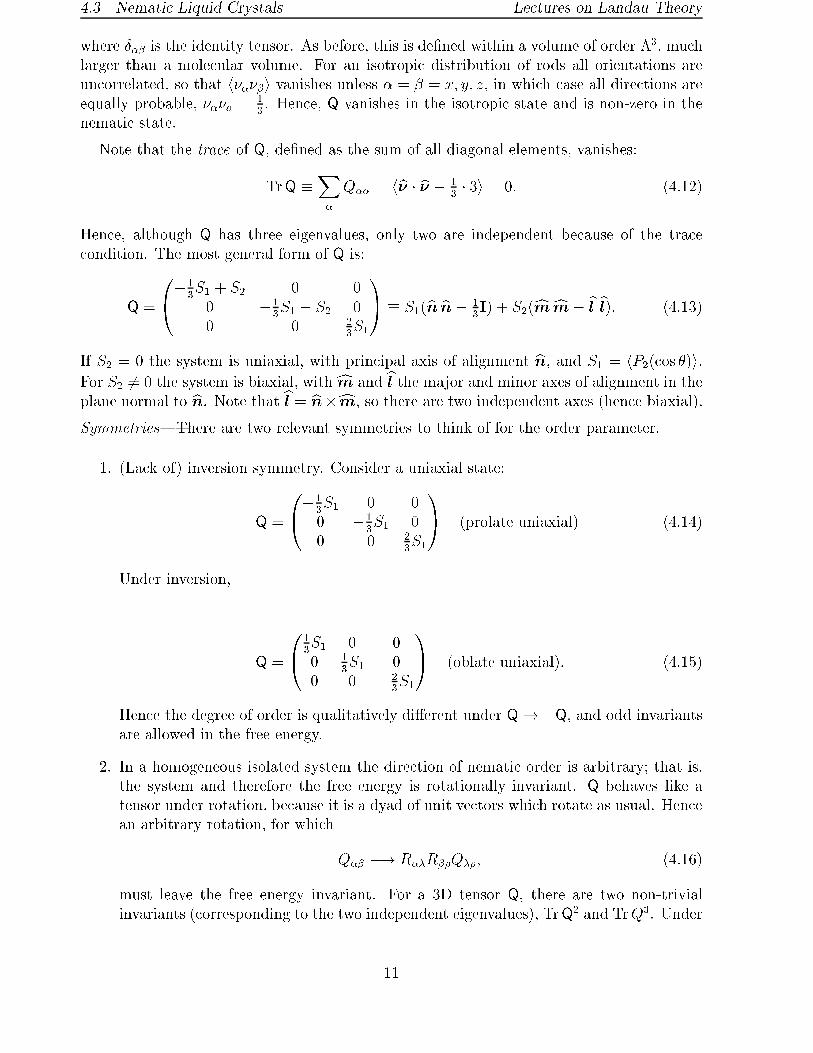
where �� is the identity tensor. As before, this is de�ned within a volume of order �3, much

larger than a molecular volume. For an isotropic distribution of rods all orientations are

uncorrelated, so that h����i vanishes unless � = � = x; y; z, in which case all directions are

equally probable, ���� = 13. Hence, Q vanishes in the isotropic state and is non-zero in the

nematic state.

Note that the trace of Q, de�ned as the sum of all diagonal elements, vanishes:

TrQ �X�

Q�� = hb� � b� � 13� 3i = 0: (4.12)

Hence, although Q has three eigenvalues, only two are independent because of the trace

condition. The most general form of Q is:

Q =

0@�13S1 + S2 0 0

0 �13S1 � S2 0

0 0 23S1

1A � S1(bn bn� 13I) + S2(cmcm� bl bl): (4.13)

If S2 = 0 the system is uniaxial, with principal axis of alignment bn, and S1 = hP2(cos �)i.For S2 6= 0 the system is biaxial, withcm and bl the major and minor axes of alignment in the

plane normal to bn. Note that bl = bn�cm, so there are two independent axes (hence biaxial).

Symmetries|There are two relevant symmetries to think of for the order parameter.

1. (Lack of) inversion symmetry. Consider a uniaxial state:

Q =

0@�13S1 0 0

0 �13S1 0

0 0 23S1

1A (prolate uniaxial) (4.14)

Under inversion,

�Q =

0@13S1 0 0

0 13S1 0

0 0 �23S1

1A (oblate uniaxial): (4.15)

Hence the degree of order is qualitatively di�erent under Q! �Q, and odd invariants

are allowed in the free energy.

2. In a homogeneous isolated system the direction of nematic order is arbitrary; that is,

the system and therefore the free energy is rotationally invariant. Q behaves like a

tensor under rotation, because it is a dyad of unit vectors which rotate as usual. Hence

an arbitrary rotation, for which

Q�� �! R��R��Q��; (4.16)

must leave the free energy invariant. For a 3D tensor Q, there are two non-trivial

invariants (corresponding to the two independent eigenvalues), TrQ2 and TrQ3. Under

11

4.3 Nematic Liquid Crystals Lectures on Landau Theory

a rotation,

TrQ �Q = Q�� Q�� ! R��R��Q��R��R�� Q�� (4.17a)

= (RTR)�� (RTR)��Q��Q�� (4.17b)

= �� ��Q��Q�� (4.17c)

= Q��Q�� (4.17d)

= TrQ � Q; (4.17e)

and similarly for any power TrQn.

Free Energy|Respecting the invariants, the free energy is

fL = 12a (T � T�) TrQ

2 + 13bTrQ3 + 1

4c�TrQ2

�2: (4.18)

We can now insert the general form of Q, Eq. (4.13), into the free energy, and minimize over

S1 and S2. We need to compute quantities such as

TrQ2 = S21 Tr

�bnbn� 1

3I

�2

+ 2S1S2Tr

�bnbn� 1

3I

���cmcm� bl bl� + S

22 Tr

�cmcm� bl bl�2= 1

3S21 Tr[bnbn+ 1

3I]� 2

3S1S2Tr

�cmcm� bl bl�+ S22 Tr[cmcm+ bl bl] (4.19a)

= 23S21 + 2S2

2 ; (4.19b)

using properties of unit vectors and the orthonormal system fbn;cm;blg. The free energy

reduces to (up to algebraic errors!)

fL = 13a(T � T�)S

21 +

227b S

31 +

19c S

41| {z }

F1

+S22

�a(T � T�)� 4

3b S1 +

23c S

22

�+ c S

42| {z }

F2

: (4.20)

Order Parameter S1

Fre

e E

nerg

y

TIN

Thermodynamics In principle we must look for minima of fL as a function of S1 and S2. F1

gives, for S2 = 0, a minima at T > T� for bS1 negative, due to the cubic term. This will

12

4.3 Nematic Liquid Crystals Lectures on Landau Theory

make the term in square brackets in F2 positive, so the system is stable against S2 becoming

non-zero, and is in fact a uniaxial state. So, we consider S2 = 0 and minimize over S1:�@F1

@S1

�S2=0

= 0 �! S�1 =

8<:01

4c

h�b�

pb2 � 24ac

i:

(4.21)

By inspection, we take the root with the largest magnitude; now we must change the tem-

perature until the free energy at S1� vanishes, at which point the system makes a �rst order

phase transition to the nematic state. (Somewhat tedious) algebra gives:

S1� = � b

6c; �T = TIN � T� =

b2

27ac: (4.22)

If want a prolate uniaxial state we must have S1 positive, in which case we must choose

b < 0. Conventionally, then, the Landau Free energy for a nematic liquid crystal is usually

written as fL = : : :� 13bTrQ3+ : : : , with b > 0. We'll continue here, however, with a general

b. Substituting into the free energy, we �nd

f = f0 +

(0 (T > TIN)12a(T � T�)S

21� + : : : (T � TIN):

(4.23)

The free energy is continuous at TIN , but has a kink. This kink is related to the entropy

change, for we can calculate

S

V= � @f

@T= �@f0

@T+

(0 (T > TIN)@@T

�12a(T � T�)S

21� + : : :

(T � TIN ):

(4.24)

Hence the entropy change upon cooling through the transition temperature is

�S = ST=T�IN� ST=T+

IN= � b

4

729 a c3(4.25)

The entropy of the system decreases, which is the latent heat L = TIN�S liberated upon

cooling into the nematic state.

Notes:

1. Like the magnet, the liquid crystal spontaneously breaks rotational symmetry, with a

direction (director) bn chosen at random by the system.

2. The Landau free energy for a �rst order transition is not strictly correct just below

the transition, since the order parameter grows from a �nite value. Hence all results

can only be qualitative at best, even within mean �eld theory. Conversely, the Landau

energy for a second order transition is exact, within mean �eld theory, close to the

transition.

3. There are three parameters, a; b; c; T�, which can be �tted from experiment by measur-

ing, for example, TIN ; S1�;�T , and the latent heat. �T can be measured from light

scattering far above TIN .

13

4.4 Crystal Systems Lectures on Landau Theory

4. Other mean �eld �rst order phase transitions also typically have a cubic term (e.g.

most crystal phases).

Biaxial Phases|Consider the case where the cubic term vanishes, b = 0. One could imagine

such a system by, for example, mixing molecules of di�erent shapes. In this case the free

energy is all even terms in S1 and S2:

fL = 13a(T � T�)S

21 +

19c S

41 + S

22

�a(T � T�) +

23c S

22

�+ c S

42 : (4.26)

This is thus a second order phase transition, and it turns out to have both S1 and S2 non-

zero, so it is a biaxial phase transition. There have been very few examples of biaxial phases;

one can see that the chemistry has to be very special for such a phase.

−0.4 −0.2 0 0.2 0.4

Cubic Term b

S1

prolate uniaxial oblate uniaxial

biaxial

4.4 Crystal Systems

With crystal systems we will round o� the most common set of classical phase transitions.

In this case the order parameter is the density (or modulation of some other quantity, such

as composition, charge, etc))

�(r) = ��+Xq2G

��(q)e�iq�r + c:c

�; (4.27)

The Landau free energy is usually expanded in the Fourier coeÆcients of the density, �(q).

Note that these are complex numbers, and hence contain phase information. In particular,

note that ��(q) = �(�q), which can be seen by taking the complex conjugate of �(r), which

must be the same thing as �(r) (a real number).

4.4.1 Lamellar Systems

Lamellar systems are one-dimensional crystals, and include magnetic systems, smectic liquid

crystals, and lamellar block copolymers. A wavevector is assumed, q = 2�bn=�, pointing ina direction bn with wavelength �.

14

4.4 Crystal Systems Lectures on Landau Theory

Order Parameter|The order parameter is taken to be the single Fourier mode �(q). Other

harmonics will be stabilized at lower temperatures. This is an assumption, and in some cases

one could have, due to the microscopic physics, a coincidence of transition temperatures for

several harmonics.

Symmetries|The only relevant symmetry is translational invariance. Although we will see

that the lamellar state breaks translational invariance, the lamellae can be slid anywhere, and

the high temperature state has no preferred point of reference. Under translation r! r+a,

the density transforms to

�(r)! �(r + a) = �� +Xq2G

��(q)e�iq�r�iq�a + c:c

�: (4.28)

Hence we have �(q)! �(q)e�iq�a. That is, all Fourier modes pick up a phase shift. For the

free energy to possess translational invariance, there can be no dependence on the complex

phase of the Fourier modes.

Free Energy|So, we now expand in a single Fourier mode. The lowest order expansion of

the Landau free energy is

fL =1

2a(T � Tc)�q��q +

1

4b (�q��q)

2(4.29a)

=1

2a(T � Tc) j�qj2 + 1

4b j�qj4 : (4.29b)

Since the free energy only depends on the modulus of �(q), there is no dependence on

the phase. There is no cubic term, since we always assume an analytic expansion of the

free energy, which precludes terms like j�(q)j3=2. Hence, one-dimensional crystals are, within

mean �eld theory, continuous transitions, with spontaneously broken translational symmetry.

That is, the direction is arbitrary, as is the phase of the lattice. We will see later that this

transition is ripe for all sorts of interesting uctuation e�ects.

4.4.2 Two and Three Dimensional Crystals

Order Parameter| Consider �rst a 2-dimensional hexagonal crystal. In this case there are

three wavevectors in the �rst harmonicG� = fq1;q2;q3g, of equal magnitude and at relative

angles of 60Æ and 120Æ degrees. They form a star of wavevectors. The Landau free energy

for the transition to a hexagonal crystal must thus be expanded in this star:

�(r) = ��+Xq2G�

��(q)e�iq�r + c:c

�; (4.30)

Free Energy|As with the lamellar crystal, the free energy must be constructed so that

it is translationally invariant, and doesn't depend on the absolute position of the lattice.

Consider the transformation of the following terms under a translation, r! r+ a:

�k1�k2 �! �k1�k2 e�i(k1+k2)�a (4.31a)

�k1�k2�k3 �! �k1�k2�k3 e�i(k1+k2+k3)�a (4.31b)

�k1�k2�k3�k4 �! �k1�k2�k3�k4 e�i(k1+k2+k3+k4)�a (4.31c)

15

4.4 Crystal Systems Lectures on Landau Theory

Hexagonal lattice and its star of wavevectors 2 distinct triangles (cubic terms)

Two distinct familiesof quartic terms

We can have quadratic terms in the free energy for combinations of Fourier modes for which

k1 + k2 = 0 , cubic terms for combinations for which which k1 + k2 + k3 = 0, and quartic

terms for combinations for which k1+k2+k3+k4 = 0. Note that these are vector sums of the

allowable wavevectors in the star for the relevant crystal, in this case the hexagonal crystal.

Hence it's easiest to �nd which terms are allowed by constructing the allowable triangles (for

the cubic terms) and quadrangles (for the quartic terms) from the star of wavevectors.

Hence we have the following terms in the free energy:

�1��1; �2��2; �3��3; 3 quadratic terms (4.32a)

�1��2�3; ��1�2��3 2 distinct triangles (4.32b)

�1�2��1��2 : : : 3 open quadrangles (4.32c)

�1��1�1��1 : : : 3 double quadratic terms: (4.32d)

Now, we assume a symmetry between all three wavevectors, since the system is rotationally

invariant. That is, we'll assume the magnitude of each Fourier mode is the same:

�1 = ei�1 ; �2 = e

i�2 ; �3 = ei�3 ; (4.33)

where is the magnitude and �i are arbitrary (so far) phase factors.

Hence all three quadratic terms must be equivalent, and have the same coeÆcient in

the free energy. Similarly, all three cubic terms are the same, so they must have the same

coeÆcient. However, the two classes of quartic terms are distinctly di�erent, and each can,

potentially, have its own separate coeÆcient. So, we are led to the following free energy:

fL = 12a (T � T�)

2 + 13b

3 cos (�1 � �2 + �3) +14(c1 + c2)

4: (4.34)

16

4.4 Crystal Systems Lectures on Landau Theory

In a purely phenomenological approach we might as well set c1+c2 = c, another arbitrary

constantz. In some systems (notably block copolymers) c1 and c2 can be calculated from

\�rst principles", assuming Gaussian chains. The phase factors are chosen to minimize the

free energy: choosing �1 � �2 + �3 = 0 gives the largest magnitude for the cosine, so the

cubic term can then contribute to the free energy for a non-zero (note that the sign of

doesn't have any physical signi�cance). Note that the phase factors cannot be determined

to any more precision: higher order terms in the free energy lead to a unique determination

of the relative phases.

Notes|

1. All real three dimensional crystals have �rst order phase transitions because \triangles"

can be made. Note that a 2D square lattice has, within mean �eld theory, a continuous

phase transition!

2. One expects single-starred crystals (i.e. square instead of rectangular, hexagonal in-

stead of rhombic) to appear from the melt, since these will typically be triggered by the

�rst length scale which becomes unstable. For deeper quenches, or strong �rst order

phase transitions, other harmonics develop.

3. By counting the number of triangles, essentially, one can make a very beautiful and

general argument that most simple substances should become BCC crystals immedi-

ately from the meltx. This simple rule is obeyed astonishingly often!

4. An excellent example of this approach combined with a derivation of the Landau coef-

�cients is Leibler's treatment of microphase separation in block copolymers{. He pre-

dicted the stability of BCC, hexagonal, and lamellar phases from a single-star theory.

Enlarging the theory to include the second star (harmonic) can predict the stability of

the Gyroid phasek

zFor higher order terms the di�erent classes of pentangles, sextangles, etc could have di�erent phase

factors, in which case the corresponding coeÆcients should be kept distinct.xS. Alexander and J. McTague, \Should all crystals be bcc? Landau theory of solidi�cation and crystal

nucleation", Phys. Rev. Lett. 41 (1978) 702-705{L. Leibler, \Theory of Microphase Separation in Block Copolymers", Macromolecules 13 (1980) 1602-

1617kS. T. Milner and P. D. Olmsted, \Analytical weak-segregation theory of bicontinuous phases in diblock

copolymers", J. Phys. II (France) 7 (1997) 249-255.

17

5. Smectic Liquid Crystals Lectures on Landau Theory

5 Smectic Liquid Crystals

5.1 Mean Field Theory of the Nematic-Smectic{A transition

A thermotropic smectic liquid crystal has the symmetry of a one-dimensional lamellar crystal,

but su�ers the complications of occuring out of a nematic phase which has broken rotational

symmetry. In the smectic{A phase the rodlike molecules are, on average, parallel to the

layer normals. Hence the director, bn(r), is parallel to the layer normal.

Order Parameter|The order parameter of the smectic transition is taken to be the Fourier

component of the fundamental harmonic of the one-dimensional crystal; i.e. we expand the

density as

�(r) = �� +� e

�iq bn�r + �eiq n�r

; (5.1)

where bn is both the director and the de�nition of the layer normals.

n

z

x

θn

Symmetries| The layers can be oriented in any direction, as long as the director is also

pointing in that direction. Hence any smectic free energy that we write down must be

invariant under simultaneous rotations of the layers and the director. Under a uniform

rotation of a smectic system about the by axis by an angle �, the director changes:

bn �! bn0= bn+ Æbn = bn� � bx: (5.2)

Hence the smectic order parameter changes according to:

�! eiq �x = e

�iqx Ænx : (5.3)

Any free energy we write down my respect this symmetry (rotational invariance).

Free Energy|Now we write down the free energy. First we consider a uniform amplitude of

the density modulation . Since a smectic is a one-dimensional crystal, we can reproduce

what we had before:

fL;hom = 12a(T � Tc) j j2 + 1

4c j j4 : (5.4)

18

5.2 Free Energy and Superconducting Analogy Lectures on Landau Theory

To this we add the energy of deformation of the director uctuations, the Frank Free Energy:

fN = 12K1 (r � Æbn)2 + 1

2K2 (bn �r� Æbn)2 + 1

3K3 jbn� (r� Æbn)j2 ; (5.5)

where K1; K2; K3 penalize, respectively, splay, bend, and twist uctuations.

Finally, we can consider an envelope of spatial modulations in the magnitude of the density

modulation, (r). These uctuations, in the smectic state, correspond to phonons. If we

consider the rigid body rotation above, transverse spatial derivatives of pick up a term

from the director rotation:

@x (r) �!| {z }(rotate about by)

(@x ) e�iq xÆnx + iq Ænx (r) e

�iq xÆnx: (5.6)

Since the free energy must be invariant under a rigid body rotation, such spatial deriva-

tives must not contribute to the free energy. Hence the free energy of deforming the order

parameter is

fL;def =12gk jbn �r j2 + 1

2g? j(r? � iqÆbn) j2 : (5.7)

The additional term in parentheses in the second terms subtracts o� the unwanted irrelevant

term. This derivative is often called a covariant derivative, and has an analogy in super-

conductivity, in which the superconductor is analogous to the smectic order parameter and

the vector potential is analogous to the director uctuations. This is an example of a gauge

�eld theory, which arises when the relevant order parameter has a local internal symmetry

(the smectic order parameter is a complex number with a phase, corresponding to a U(1)

symmetry, which can vary from point to point). There have been many interesting fruits

born out of this analogy between smectics and superconductors! In electrodynamics there

is a gauge symmetry (the vector potential A is de�ned only up to an additive irrotational

vector �eld r�), while in the smectic liquid crystal the gauge is actually �xed because of

the presence of a director in the nematic state.

5.2 Free Energy and Superconducting Analogy

To compare the liquid crystals and superconductors, let's look at the free energies. For the

liquid crystal we have

fNA = 12a j j2 + 1

4c j j4 + 1

2gk jbn �r j2 + 1

2g? j(r? � iqÆbn) j2 + 1

2K (r�Æn̂�)

2; (5.8)

where we have used the so-called one-constant approximation K1 = K2 = K3 � K.

For a superconductor, we'll take the order parameter to be again. Landau postulated

that this is a complex number, and in fact it turns out to be closely related to the wavefunc-

tion for Cooper pairs of electrons (which is a complex number). The physics of electrons

is invariant under a local change in the phase of the wavefunction, (r) ! (r)ei�(r). This

transformation is in fact the gauge invariance which gives rise to the electromagnetic �eld,

and we usually write

(r)! (r)ei2e

Rr

r0A�dr0

; (5.9)

19

5.2 Free Energy and Superconducting Analogy Lectures on Landau Theory

where A is the electromagnetic vector potential (this funny phase factor gives rise to the

Aharonov-Bohm e�ect), in units where the speed of light is unity. There is a 2 here because

the wavefunction is for a pair of electrons. Now, we can write down the free energy for a

superconducting transition, exactly as for the smectic. When it comes to writing the gradient

terms we must \subtract" o� this arbitrary phase, which can't change the physics, so gradient

operators generally enter as ~r� i2eA. Finally, there is a free energy associated with gauge

�eld uctuations: the energy in the magnetic �eld is B � B=8�. Writing B = r � A, we

have, for the superconducting free energy,

fsup =12a j j2 + 1

4c j j4 + 1

2g

�����r� i2e

~A

�

����2 + c2

8�jr�Aj2 : (5.10)

Hence, aside from the fact that the liquid crystal is anisotropic, and the coupling of A to the

gradient terms is slightly di�erent in tensorial nature to the coupling of Æbn, the transitions\should" be qualitatively the same. Just as a superconductor expels magnetic ux, a liquid

crystal expels (it turns out) both twist and bend director uctuations. For example, it was

realized that the analog of the Abrikosov vortex phase of Type II superconductors should

exist in liquid crystals, and this was subsequently predicted and then found experimentally:

the \twisted grain boundary (TGB) phase" in cholesteric smectics.

The phase diagram of a smectic looks something like the following:

Isotropic

TNematic

???????

first order lines

tricritical point

Smectic A

-1(molecular length)

The nematic phase intervenes when the molecules are anisotropic enough, and otherwise the

system can go directly from the isotropic to the smectic phase. One can show quite generally

20

5.3 Fluctuations and the Halperin-Lubensky-Ma E�ect. Lectures on Landau Theory

that the following term, which couples liquid crystalline order to density,��

f Q = Q�� r��r�� (5.11)

leads (via nematic uctuations) to an e�ective quartic term in the smectic free energy of

the form �� 4, where � is the susceptibility for uctuations around the nematic phase.

Hence, it is likely that for molecular parameters with a narrow nematic range, for which the

susceptibility � is large, the total quartic term in the smectic free energy is negative, leading

to a �rst order phase transition. For parameters with a wide nematic range the N � A

transition is expected, within mean �eld theory, to be a continuous transition. In the next

section we will see that this does not, generally, survive inclusion of uctuations.

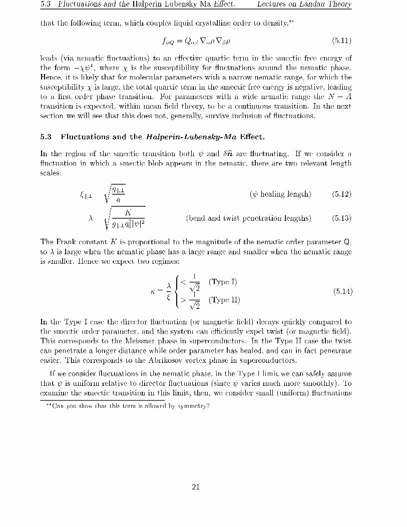
5.3 Fluctuations and the Halperin-Lubensky-Ma E�ect.

In the region of the smectic transition both and Æbn are uctuating. If we consider a

uctuation in which a smectic blob appears in the nematic, there are two relevant length

scales:

�k;? =

rgk;?

a( healing length) (5.12)

� =

sK

gk;?q20j j2

(bend and twist penetration lengths) (5.13)

The Frank constant K is proportional to the magnitude of the nematic order parameter Q,

so � is large when the nematic phase has a large range and smaller when the nematic range

is smaller. Hence we expect two regimes:

� � �

�

8><>:<

1p2

(Type I)

>1p2

(Type II)(5.14)

In the Type I case the director uctuation (or magnetic �eld) decays quickly compared to

the smectic order parameter, and the system can eÆciently expel twist (or magnetic �eld).

This corresponds to the Meissner phase in superconductors. In the Type II case the twist

can penetrate a longer distance while order parameter has healed, and can in fact penetrate

easier. This corresponds to the Abrikosov vortex phase in superconductors.

If we consider uctuations in the nematic phase, in the Type I limit we can safely assume

that is uniform relative to director uctuations (since varies much more smoothly). To

examine the smectic transition in this limit, then, we consider small (uniform) uctuations

��Can you show that this term is allowed by symmetry?

21

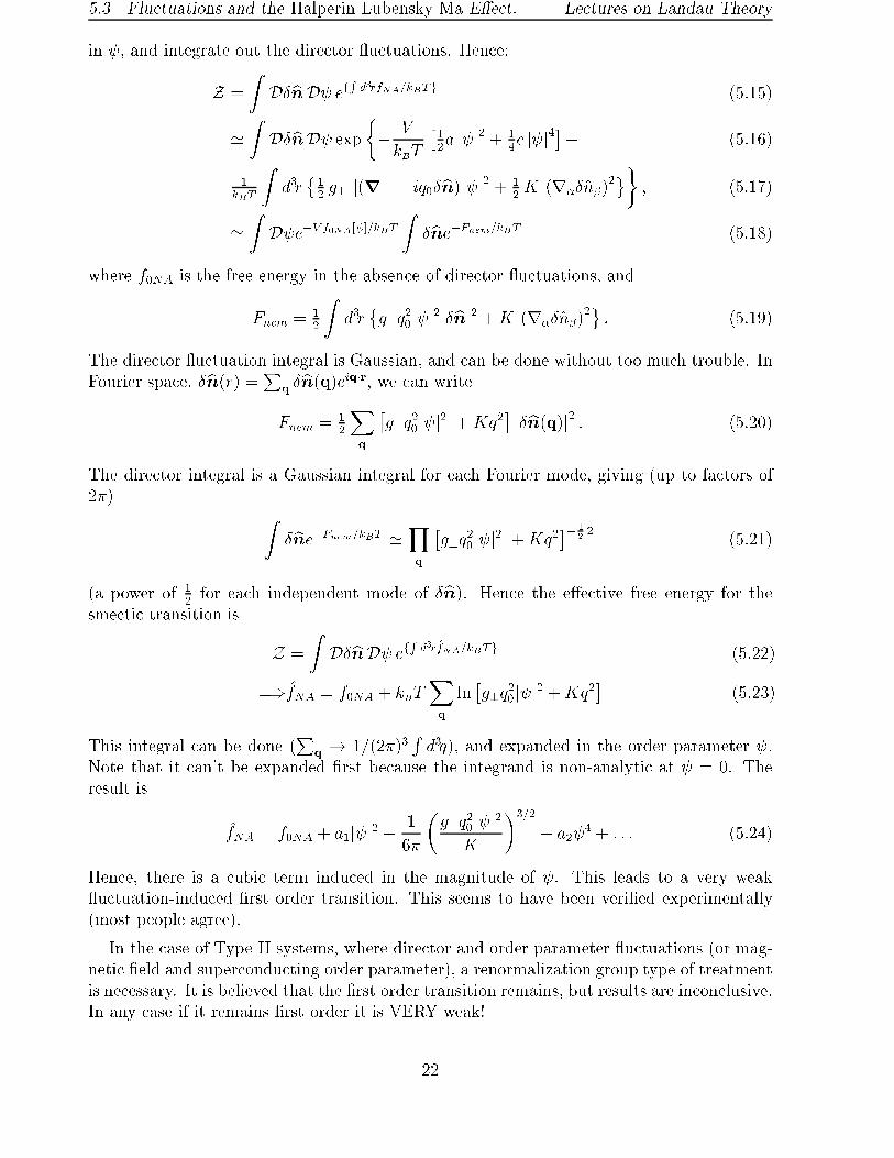
5.3 Fluctuations and the Halperin-Lubensky-Ma E�ect. Lectures on Landau Theory

in , and integrate out the director uctuations. Hence:

Z =

ZDÆbnD efR d3rfNA=kBTg (5.15)

'ZDÆbnD exp

�� V

kBT

�12a j j2 + 1

4c j j4�+ (5.16)

1kBT

Zd3r�12g? j(r? � iq0Æbn) j2 + 1

2K (r�Æn̂�)

2�

; (5.17)

'ZD e�V f0NA[ ]=kBT

ZÆbne�Fnem=kBT (5.18)

where f0NA is the free energy in the absence of director uctuations, and

Fnem = 12

Zd3r�g?q

20j j2jÆbnj2 +K (r�Æn̂�)

2: (5.19)

The director uctuation integral is Gaussian, and can be done without too much trouble. In

Fourier space, Æbn(r) =PqÆbn(q)eiq�r, we can write

Fnem = 12

Xq

�g?q

20j j2j+Kq

2� jÆbn(q)j2 : (5.20)

The director integral is a Gaussian integral for each Fourier mode, giving (up to factors of

2�) ZÆbne�Fnem=kBT 'Y

q

�g?q

20j j2j+Kq

2�� 1

22

(5.21)

(a power of 12for each independent mode of Æbn). Hence the e�ective free energy for the

smectic transition is

Z =

ZDÆbnD efR d3rf̂NA=kBTg (5.22)

=)f̂NA = f0NA + kBT

Xq

ln�g?q

20j j2 +Kq

2�

(5.23)

This integral can be done (P

q! 1=(2�)3

Rd3q), and expanded in the order parameter .

Note that it can't be expanded �rst because the integrand is non-analytic at = 0. The

result is

f̂NA = f0NA + a1j j2 � 1

6�

�g?q

20j j2K

�3=2

+ a2 4 + : : : (5.24)

Hence, there is a cubic term induced in the magnitude of . This leads to a very weak

uctuation-induced �rst order transition. This seems to have been veri�ed experimentally

(most people agree).

In the case of Type II systems, where director and order parameter uctuations (or mag-

netic �eld and superconducting order parameter), a renormalization group type of treatment

is necessary. It is believed that the �rst order transition remains, but results are inconclusive.

In any case if it remains �rst order it is VERY weak!

22

5.4 Layered liquids and the Brazovskii e�ect Lectures on Landau Theory

5.4 Layered liquids and the Brazovskii e�ect

Some day I hope Daniel will give me time to talk about this!

23