universal prediction distribution for surrogate modelsroustant/documents/m105352.pdf ·...

SIAM/ASA J. UNCERTAINTY QUANTIFICATION c© 2017 Society for Industrial and Applied MathematicsVol. 5, pp. 1086–1109 and American Statistical Association

Universal Prediction Distribution for Surrogate Models∗

Malek Ben Salem† , Olivier Roustant‡ , Fabrice Gamboa§ , and Lionel Tomaso¶

Abstract. The use of surrogate models instead of computationally expensive simulation codes is very conve-nient in engineering. Roughly speaking, there are two kinds of surrogate models: the deterministicand the probabilistic ones. These last are generally based on Gaussian assumptions. The mainadvantage of the probabilistic approach is that it provides a measure of uncertainty associated withthe surrogate model in the whole space. This uncertainty is an efficient tool to construct strategiesfor various problems such as prediction enhancement, optimization, or inversion. In this paper, wepropose a universal method to define a measure of uncertainty suitable for any surrogate model ei-ther deterministic or probabilistic. It relies on cross-validation submodel predictions. This empiricaldistribution may be computed in much more general frames than the Gaussian one; thus it is calledthe universal prediction distribution (UP distribution). It allows the definition of many samplingcriteria. We give and study adaptive sampling techniques for global refinement and an extension ofthe so-called efficient global optimization algorithm. We also discuss the use of the UP distributionfor inversion problems. The performances of these new algorithms are studied both on toy modelsand on an engineering design problem.

Key words. surrogate modeling, design of experiments, Bayesian optimization

AMS subject classifications. 62L05, 62K05, 90C26

DOI. 10.1137/15M1053529

1. Introduction. Surrogate modeling techniques are widely used and studied in engineer-ing and research. Their main purpose is to replace an expensive-to-evaluate function s by asimple response surface s also called a surrogate model or metamodel. Notice that s can be acomputation-intensive simulation code. These surrogate models are based on a given trainingset of n observations zj = (xj , yj), where 1 ≤ j ≤ n and yj = s(xj). The accuracy of thesurrogate model relies, inter alia, on the relevance of the training set. The aim of surrogatemodeling is generally to estimate some features of the function s using s. Of course one islooking for the best trade-off between good accuracy of the feature estimation and the numberof calls of s. Consequently, the design of experiments, that is the sampling of (xj)1≤j≤n, is acrucial step and an active research field.

∗Received by the editors December 18, 2015; accepted for publication (in revised form) August 28, 2017; publishedelectronically November 14, 2017.

http://www.siam.org/journals/juq/5/M105352.htmlFunding: The first author is funded by a CIFRE grant from the ANSYS company, subsidized by the French

National Association for Research and Technology (ANRT, CIFRE grant 2014/1349).†Mines de Saint-Etienne, UMR CNRS 6158, Limos, F-42023, Saint-Etienne, France and ANSYS, Inc, F-69100

Villeurbanne, France ([email protected]).‡Mines de Saint-Etienne, UMR CNRS 6158, Limos, F-42023, Saint-Etienne, France ([email protected]).§IMT Institut de Mathematiques de Toulouse, F-31062 Toulouse, Cedex 9, France ([email protected]

toulouse.fr).¶ANSYS, Inc, F-69100 Villeurbanne, France ([email protected]).

1086

http://www.siam.org/journals/juq/5/M105352.html

mailto:[email protected]





SURROGATE MODELS UNIVERSAL PREDICTION DISTRIBUTION 1087

There are two ways to sample: either drawing the training set (xj)1≤j≤n at once or build-ing it sequentially. Among the sequential techniques, some are based on surrogate models.They rely on the feature of s that one wishes to estimate. Popular examples are efficientglobal optimization (EGO) [17] and stepwise uncertainty reduction [3]. These two methodsuse Gaussian process regression also called the kriging model. It is a widely used surrogatemodeling technique. Its popularity is mainly due to its statistical nature and properties. In-deed, it is a Bayesian inference technique for functions. In this stochastic frame, it providesan estimate of the prediction error distribution. This distribution is the main tool in Gaussiansurrogate sequential designs. For instance, it allows the introduction and the computation ofdifferent sampling criteria such as expected improvement (EI) [17] or expected feasibility [4].Away from the Gaussian case, many surrogate models are also available and useful. Noticethat none of them including the Gaussian process surrogate model are the best in all circum-stances [14]. Classical surrogate models are, for instance, the support vector machine (SVM)[36], linear regression [5], moving least squares [22]. More recently a mixture of surrogates hasbeen considered in [38, 13]. Nevertheless, these methods are generally not naturally embed-dable in some stochastic frame. Hence, they do not provide any prediction error distribution.To overcome this drawback, several empirical design techniques have been discussed in theliterature. These techniques are generally based on resampling methods such as bootstrap,jackknife, or cross validation. For instance, Gazut et al. [10] and Jin, Chen, and Sudjianto[15] consider a population of surrogate models constructed by resampling the available datausing bootstrap or cross validation. Then, they compute the empirical variance of the predic-tions of these surrogate models. Finally, they sample iteratively the point that maximizes theempirical variance in order to improve the accuracy of the prediction. To perform optimiza-tion, Kleijnen, van Beers, and van Nieuwenhuyse [20] use a bootstrapped kriging varianceinstead of the kriging variance to compute the EI. Their algorithm consists in maximizingthe EI computed through bootstrapped kriging variance. However, most of these resamplingmethod-based design techniques lead to clustered designs [2, 15].

In this paper, we give a general way to build an empirical prediction distribution al-lowing sequential design strategies in a very broad frame. Its support is the set of all thepredictions obtained by the cross-validation surrogate models. The novelty of our approachis that it provides a prediction uncertainty distribution. This allows a large set of samplingcriteria.

The paper is organized as follows. We start by presenting in section 2 the backgroundand notations. In section 3 we introduce the universal prediction (UP) empirical distribution.In sections 4 and 5, we use and study features estimation and the corresponding samplingschemes built on the UP empirical distribution. Section 4 is devoted to the enhancement ofthe overall model accuracy. Section 5 concerns optimization. In section 6, we study a real lifeindustrial case implementing the methodology developed in section 4. Section 7 deals withthe inversion problem. In section 8, we conclude and discuss the possible extensions of ourwork. All proofs are postponed to section 9.

2. Background and notations.

2.1. General notation. To begin with, let s denote a real-valued function defined on X,a nonempty compact subset of the Euclidean space Rp (p ∈ N?). In order to estimate s, we

1088 M. BEN SALEM, O. ROUSTANT, F. GAMBOA, AND L. TOMASO

have at hand a sample of size n (n ≥ 2): Xn =(x1, . . . , xn

)> with xj ∈ X, j ∈ J1;nK, and

Yn =(y1, . . . , yn

)>, where yj = s(xj) for j ∈ J1;nK. We note Yn = s(Xn).Let Zn denote the observations: Zn := {(xj, yj), j ∈ J1;nK}. Using Zn, we build a

surrogate model sn that mimics the behavior of s. For example, sn can be a second orderpolynomial regression model. For i ∈ {1 . . . n}, we set Zn,−i := {(xj, yj), j = 1, . . . , n, j 6= i}and so sn,−i is the surrogate model obtained by using only the dataset Zn,−i. We will call snthe master surrogate model and (sn,−i)i=1...n its submodels.

Further, let d(., .) denote a given distance on Rp (typically the Euclidean one). For x ∈X and A ⊂ X, we set dA(x) = inf{d(x,x′) : x′ ∈ A} and if A = {x′1, . . . ,x′m} is finite(m ∈ N?), for i ∈ 1, . . . ,m let A−i denote {x′j, j = 1 . . .m, j 6= i}. Finally, we set d(A) =max{dA−i(x

′i) : i = 1, . . . ,m}, the largest distance of an element of A to its nearest neighbor.

2.2. Cross validation. Training an algorithm and evaluating its statistical performanceson the same data yields an optimistic result [1]. It is well known that it is easy to overfitthe data by including too many degrees of freedom and so inflate the fit statistics. The ideabehind cross validation (CV) is to estimate the risk of an algorithm splitting the dataset onceor several times. One part of the data (the training set) is used for training and the remainingone (the validation set) is used for estimating the risk of the algorithm. Simple validation orholdout [8] is hence a CV technique. It relies on one splitting of the data. Then one set isused as training set and the second one is used as validation set. Some other CV techniquesconsist in a repetitive generation of holdout estimators with different data splitting [11]. Onecan cite, for instance, the leave-one-out (LOO) CV (LOO-CV) and the k-fold CV (KFCV).KFCV consists in dividing the data into k subsets. Each subset plays the role of validationset while the remaining k − 1 subsets are used together as the training set. The LOO-CVmethod is a particular case of KFCV with k = n.

For i = 1, . . . , n, the LOO error is εi = sn,−i(xi) − yi, where the submodels sn,−i areintroduced in section 2.1. In our study, we are interested in the distribution of the localpredictor for all x ∈ X (x is not necessarily a design point). As explained in the next section,the CV paradigm provides submodels allowing the definition of a local uncertainty measure forthe master surrogate model sn. This distribution is estimated by using LOO-CV predictions.This is one of the easiest ways to build an uncertainty measure based on resampling.

3. UP distribution.

3.1. Overview. As discussed in the previous section, CV is used as a method for estimat-ing the prediction error of a given model. In our case, we introduce a novel use of CV in orderto estimate the local uncertainty of a surrogate model prediction. Hence, for a given surrogatemodel s and for any x ∈ X, sn,−1(x), . . . , sn,−n(x) define an empirical distribution of s(x) atx. In the case of an interpolating surrogate model and a deterministic simulation code s, it isnatural to enforce a zero variance at design points. Consequently, when predicting on a designpoint xi we have to neglect the prediction sn,−i. This can be achieved by introducing weightson the empirical distribution. These weights avoid the pessimistic submodel predictions thatmight occur in a region while the global surrogate model fits the data well in that region.


Let F (0)n,x =

∑ni=1w

0i,n(x)δsn,−i(x)(dy) be the weighted empirical distribution based on the

n different predictions of the LOO-CV submodels {sn,−i(x)}1≤i≤n and weighted by w0i,n(x)

defined in (3.1):

(3.1) w0i,n(x) =

1

n− 1if xi 6= arg min{d(x,xj), j = 1, . . . , n},

0 otherwise.

For i = 1, . . . , n, let Ri be the Voronoi cell of the point xi. The weights can be written asw0i,n(x) = 1−1Ri (x)∑n

j=1(1−1Rj (x)) , where 1Ri is the indicator function on Ri. Such binary weights lead

to unsmooth design criteria. In order to avoid this drawback, we smooth the weights. Directsmoothing based on convolution would lead to the computations of Voronoi cells. We preferto use a simpler technique. Indeed, w0

i,n(x) can be seen as a Nadaraya–Watson weight withthe kernel 1 − 1Rj (x) = 1Ri(xi) − 1Rj (x). Instead of the unsmooth indicator function 1Ri ,we use the Gaussian kernel, but other smooth kernels could also be used. This leads to thefollowing weights

(3.2) wi,n(x) =1− e−

d(x,xi)2

ρ2

n∑j=1

(1− e−

d(x,xj)2

ρ2) .

Notice that wi,n(x) increases with the distance between the ith design point xi and x.In fact, the least weighted prediction is sn,−pnn(x), where pnn(x) is the index of the nearestdesign point to x. In general, the prediction sn,−i is locally less reliable in a neighborhood ofxi. The proposed weights determine the local relative confidence level of a given submodelprediction. The term “relative” means that the confidence level of one submodel predictionis relative to the remaining submodel predictions due to the normalization factor in (3.2).The smoothing parameter ρ tunes the amount of uncertainty of sn,−i in a neighborhood of xi.Several options are possible to choose ρ. It can be either related to the distance of a point toits nearest neighbor or common for all the points. We suggest using ρ? = d(Xn). Indeed, thisis a well-suited choice for practical cases.

Definition 3.1. The universal prediction distribution (UP distribution) is the weighted em-pirical distribution

(3.3) µ(n,x)(dy) =n∑i=1

wi,n(x)δsn,−i(x)(dy).

This probability measure is nothing more than the empirical distribution of all the pre-dictions provided by CV submodels weighted by local smoothed masses.

Definition 3.2. For x ∈ X we call σ2n(x) (3.5) the local UP variance and mn(x) (3.4) the

UP expected value:

(3.4) mn(x) =∫yµ(n,x)(dy) =

n∑i=1

wi,n(x)sn,−i(x),

(3.5) σ2n(x) =

∫(y − mn(x))2 µ(n,x)(dy) =

n∑i=1

wi,n(x)(sn,−i(x)− mn(x))2.


−3 −2 −1 0 1 2 3

0.0

0.2

0.4

0.6

0.8

1.0

SVM

x

y

−3 −2 −1 0 1 2 3

0.0

0.2

0.4

0.6

0.8

1.0

Kriging

x

y

Figure 1. Illustration of the UP distribution for an SVM surrogate (left) and a kriging surrogate (right).Dashed lines: CV submodel prediction; solid red line: master model prediction; horizontal bars: local UPdistribution at xa = −1.8 and xb = 0.2; black squares: design points.

3.2. Illustrative example. Let us consider the Viana function defined over [−3, 3],

(3.6) f(x) =10 cos(2x) + 15− 5x+ x2

50.

Let Zn = (Xn,Yn) be the design of experiments such that

Xn = (x1 = −2.4,x2,= −1.2, x3 = 0, x4 = 1.2, x5 = 1.4, x6 = 2.4, x7 = 3)

and Yn = (y1, . . . , y7) their image by f . We used a Gaussian process regression [27, 21, 18]with constant trend function and Matern 5/2 covariance function s and an SVM regression[36]. We display in Figure 1 the design points, the CV submodel predictions sn,−i, i = 1, . . . , 7,and the master model prediction sn of each surrogate model.

Notice that in the interval [1, 3] (where we have 4 design points) the discrepancy betweenthe master model and the CV submodels prediction is smaller than in the remaining space.Moreover, we displayed horizontally the UP distribution at xa = −1.8 and xb = 0.2 to illustratethe weighting effect. One can notice that

• at xa the least weighted predictions are sn,−1(xa) and sn,−2(xa). These predictions donot use the two closest design points to xa: x1 (respectively, x2);• at xb, sn,−3(xb) is the least weighted prediction.

Furthermore, we display in Figure 2 the master model prediction and the region delimitedby sn(x) + 3σn(x) and sn(x)− 3σn(x). Contrary to the Gaussian case, this region cannot beinterpreted as the 99.7% traditional prediction interval. Nevertheless, it can be interpreted asa prediction interval with level greater than or equal to 88.8%. Indeed, Chebyshev’s inequalitystates that for any squared integrable random variable X and k > 0, Pr(|X − µ| ≥ kσ) ≤ 1

k2 .In particular, Pr(|X − µ| < 3σ) ≥ 1− 1

32 ≈ 88.8%.Notice that here the UP standard deviation is null at design points for the interpolating

surrogate model. In addition, its local maxima in the interval [1, 3] (where we have greaterdesign points density) are smaller than its maxima in the remaining space region.


−3 −2 −1 0 1 2 3

0.0

0.2

0.4

0.6

0.8

1.0

SVM

x

y

−3 −2 −1 0 1 2 3

0.0

0.2

0.4

0.6

0.8

1.0

Kriging

x

y

Figure 2. Uncertainty quantification based on the UP distribution for an SVM surrogate (left) and akriging surrogate (right). Blue solid line: master model prediction sn(x); light blue area: region delimited bysn(x)± 3σn(x).

0.0 0.5 1.0 1.5

0.0

0.5

1.0

1.5

2.0

2.5

3.0

Figure 3. UP-variance for kriging. Black squares: design points; blue line: sn(x); light blue: area delimitedby sn(x)± 3σn(x); light red: area delimited by sn(x)± 3σGP (x).

3.3. UP distribution in action.Case of the kriging surrogate model. Without loss of generality, let us consider the simple

kriging framework. Recall that the conditional mean and variance are given by

m(x) = k(x)>K−1n Yn,

σ2GP (x) = k(x,x)− kn(x)>K−1

n kn(x),(3.7)

where k(x,x′) is a covariance function, kn(x) is the vector (k(x,x1), . . . , k(x,xn))>, and Kn

is the invertible matrix with entries ki,j = k(xi,xj) for 1 ≤ i, j ≤ n.Notice that for an interpolating kriging, both kriging variance and UP variance vanish at

design points. Further, kriging variance does not depend on the output values once the kernelparameters are fixed; however, UP variance does. It is not everywhere smaller or larger thankriging variance; for instance, consider the toy example in Figure 3.

On one hand UP variance is a maximum in the interval [0.4, 1.3]. Indeed, if we removeone point in that region we significantly increase the variability of the submodel predictions.Similarly, UP variance is minimum in the nearly linear region [0, 0.4] ∪ [1.3, 2]. On the other


−1.0 −0.5 0.0 0.5 1.0

−1.0

−0.5

0.0

0.5

1.0

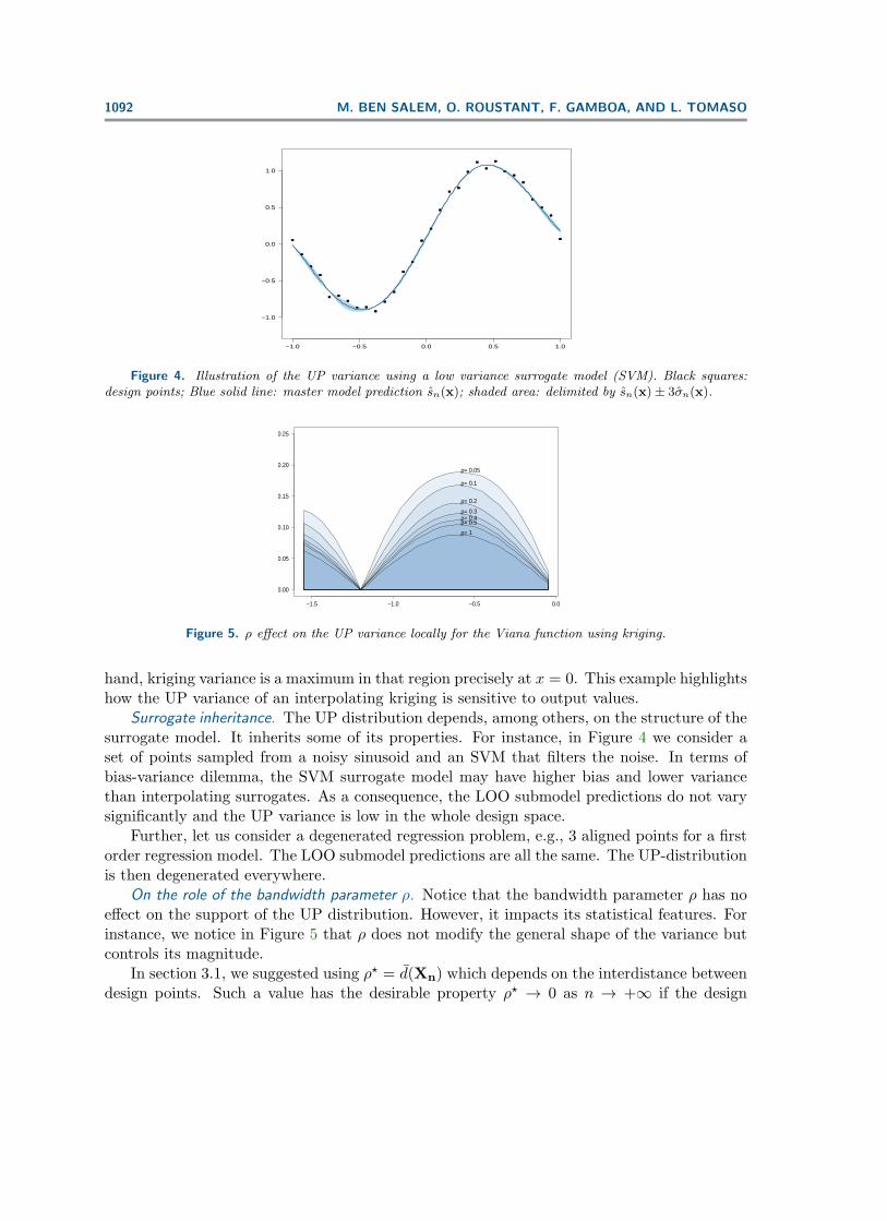
Figure 4. Illustration of the UP variance using a low variance surrogate model (SVM). Black squares:design points; Blue solid line: master model prediction sn(x); shaded area: delimited by sn(x)± 3σn(x).

−1.5 −1.0 −0.5 0.0

0.00

0.05

0.10

0.15

0.20

0.25

ρ= 0.05

ρ= 0.1

ρ= 0.2

ρ= 0.3ρ= 0.4ρ= 0.5

ρ= 1

Figure 5. ρ effect on the UP variance locally for the Viana function using kriging.

hand, kriging variance is a maximum in that region precisely at x = 0. This example highlightshow the UP variance of an interpolating kriging is sensitive to output values.

Surrogate inheritance. The UP distribution depends, among others, on the structure of thesurrogate model. It inherits some of its properties. For instance, in Figure 4 we consider aset of points sampled from a noisy sinusoid and an SVM that filters the noise. In terms ofbias-variance dilemma, the SVM surrogate model may have higher bias and lower variancethan interpolating surrogates. As a consequence, the LOO submodel predictions do not varysignificantly and the UP variance is low in the whole design space.

Further, let us consider a degenerated regression problem, e.g., 3 aligned points for a firstorder regression model. The LOO submodel predictions are all the same. The UP-distributionis then degenerated everywhere.

On the role of the bandwidth parameter ρ. Notice that the bandwidth parameter ρ has noeffect on the support of the UP distribution. However, it impacts its statistical features. Forinstance, we notice in Figure 5 that ρ does not modify the general shape of the variance butcontrols its magnitude.

In section 3.1, we suggested using ρ? = d(Xn) which depends on the interdistance betweendesign points. Such a value has the desirable property ρ? → 0 as n → +∞ if the design


of experiment is dense in the design space. This choice guarantees the convergence of thesequential algorithms presented in sections 4 and 5.

Computational aspects. When the number of design points is large, the computationalcost can be a drawback. In fact, the construction time of the submodels is O(nT ), where n isthe number of data and T is the construction time of one submodel. Nevertheless, for somesurrogate models, closed form formulas are available for the LOO-submodel predictions. Forinstance, Chevalier, Ginsbourger, and Emery [43] presented a formula for kriging. Anotherway to reduce the computational cost is to use parallel computing where each submodel iscomputed on a separate thread. Finally, we can replace the use of LOO-CV by the KFCV.

4. Sequential refinement. In this section, we use the UP distribution to define an adap-tive refinement technique called the UP-based surrogate modeling adaptive refinement tech-nique UP-SMART.

4.1. Introduction. The main goal of sequential design is to minimize the number of callsof a computationally expensive function. Gaussian surrogate models [18] are widely usedin adaptive design strategies. Indeed, Gaussian modeling gives a Bayesian framework forsequential design. In some cases, other surrogate models might be more accurate althoughthey do not provide a theoretical framework for uncertainty assessment. We propose here anew universal strategy for adaptive sequential design of experiments. The technique is basedon the UP distribution, so, it can be applied to any type of surrogate model.

In the literature, many strategies have been proposed to design the experiments (for anoverview, the interested reader is referred to [12, 40, 34]). Some strategies, such as Latinhypercube sampling [28], maximum entropy design [35], and maximin distance designs [16]are called one-shot sampling methods. These methods depend neither on the output valuesnor on the surrogate model. However, one would naturally expect to design more points in theregions with high nonlinear behavior. This intuition leads to adaptive strategies. A design ofexperiments approach is said to be adaptive when information from the experiments (inputsand responses) as well as information from surrogate models are used to select the location ofthe next point.

By adopting this definition, adaptive design of experiments methods include, for instance,surrogate model-based optimization algorithms, probability of failure estimation techniques,and sequential refinement techniques. Sequential refinement techniques aim at creating a moreaccurate surrogate model. For example, Lin et al. [25] use multivariate adaptive regressionsplines and kriging models with the sequential exploratory experimental design method. Itconsists in building a surrogate model to predict errors based on the errors on a test set. Goelet al. [13] use a set of surrogate models to identify regions of high uncertainty by computingthe empirical standard deviation of the predictions of the ensemble members. Our method isbased on the predictions of the CV submodels. In the literature, several CV-based techniqueshave been discussed. Li and Azarm [23] propose to add the design point that maximizesthe accumulative error (AE). The AE on x ∈ X is computed as the sum of the LOO-CVerrors on the design points weighted by influence factors. This method could lead to clusteredsamples. To avoid this effect, the authors [24] propose to add a threshold constraint in themaximization problem. Busby, Farmer, and Iske [6] propose a method based on a grid andCV. It affects the CV prediction errors at a design point to its containing cell in the grid.


Then, an entropy approach is performed to add a new design point. More recently, Xu et al.[42] suggest the use of a method based on Voronoi cells and CV. Kleijnen and Van Beers [19]propose a method based on the jackknife’s pseudovalues predictions variance. Jin, Chen, andSudjianto [15] present a strategy that maximizes the product between the deviation of CVsubmodel predictions with respect to the master model prediction and the distance to thedesign points. Aute et al. [2] introduce the space-filling CV trade-off approach. It consists inbuilding a new surrogate model over LOO-CV errors and then adding a point that maximizesthe new surrogate model prediction under some space-filling constraints. In general CV-basedapproaches tend to allocate points close to each other resulting in clustering [2]. This is notdesirable for deterministic simulations.

4.2. UP-SMART. The idea behind UP-SMART is to sample points where the UP dis-tribution variance (3.5) is maximal. Most of the CV-based sampling criteria use CV errors.Here, we use the local predictions of the CV submodels. Moreover, notice that the UP vari-ance is null on design points for interpolating surrogate models. Hence, UP-SMART does notnaturally promote clustering.

However, σ2n(x) can vanish even if x is not a design points. To overcome this drawback,

we add a distance penalization. This leads to the UP-SMART sampling criterion γn (4.1)

(4.1) γn(x) = σ2n(x) + δdXn

(x),

where δ > 0 is called the exploration parameter. One can set δ as a small percentage of theglobal variation of the output. UP-SMART is the adaptive refinement algorithm consistingin adding at step n a point xn+1 ∈ arg maxx∈X(γn(x)).

4.3. Performances on a set of test functions. In this subsection, we present the perfor-mance of the UP-SMART. We present first the used surrogate models.

4.3.1. Used surrogate models.Kriging. Kriging [27] or Gaussian process regression is an interpolation method. Universal

kriging fits the data using a deterministic trend and is governed by prior covariances. Letk(x,x′), be a covariance function on X × X, and let (hi)1≤i≤p be the basis functions of thetrend. Let us denote h(x) by the vector (h1(x), .., hp(x))> and let H be the matrix withentries hij = hj(xi), 1 ≤ i, j ≤ n. Furthermore, let kn(x) be the vector (k(x,x1), .., k(x,xn))>

and Kn the matrix with entries ki,j = k(xi,xj) for 1 ≤ i, j ≤ n.Then, the conditional mean of the Gaussian process with covariance k(x,x′) and its vari-

ance are given in (4.2), (4.3),

mGn(x) = h(x)>β + kn(x)>K−1n (Y −H>β),(4.2)

σ2GPn(x) = k(x,x)− kn(x)>K−1

n kn(x)> + V(x)>(H>K−1n H)−1V(x),(4.3)

β = (H>K−1n H)−1H>K−1

n Y and V(x) = h(x)> + kn(x)>K−1n H.(4.4)

Note that the conditional mean is the prediction of the Gaussian process regression. Fur-ther, we used two kriging instances with different sampling schemes in our test bench. Bothuse a constant trend function and a Matern 5/2 covariance function. The first design is ob-tained by maximizing the UP distribution variance (3.5). And the second one is obtained bymaximizing the kriging variance σ2

GPn(x).


Table 1Used test functions.

Function Dimension d n0 Nmax NtViana 1 5 7 500Branin 2 10 10 1600Camel 2 20 10 1600Extended Rosenbrock 6→10 60 100 10000Hartmann 6-dim 6→10 100 100 10000

Genetic aggregation. The genetic aggregation response surface is a method that aims atselecting the best response surface for a given design of experiments. It uses several surrogatemodels. In our examples, we use several kriging and SVM models with different settings(kernels, trend functions, . . .) and select the best weighted aggregation:

(4.5) Am(x) =m∑l=1

ωls(l)(x).

s(l) are the surrogate models and the weights ωl are computed in order to minimize acriterion combining CV errors, surrogate model errors, and a smoothness penalty. The useof such a response surface, in this test bench, aims at checking the universality of the UPdistribution: the fact that it can be applied for all types of surrogate models.

4.3.2. Test bench. In order to test the performances of the method we launched differentrefinement processes for the following set of test functions:

• Branin: fb(x1, x2) = (x2 − ( 5.14π2 )x2

1 + ( 5π )x1 − 6)2 + 10(1− ( 1

8π )) cos(x1) + 10.

• Six-hump camel: fc(x1, x2) = (4− 2.1x21 + x4

13 )x2

1 + x1x2 + x22(4x2

2 − 4).• Hartmann6: fh(X = (x1, . . . , x6)) = −

∑4i=1 αi exp(−

∑6j=0Aij(xj − Pij)2). A,P , and

α can be found in [9].• Viana: (3.6)

For each function we generated by optimal Latin hypersampling design the number ofinitial design points n0, the number of refinement points Nmax. We also generated a set of Nt

test points and their response Z(t) = (X(t), Y (t)). The used values are available in Table 1.We fixed n0 in order to get nonaccurate surrogate models at the first step. Usually, one

follows the rule-of-thumb n0 = 10 × d proposed in [26]. However, for Branin and Vianafunctions, this rule leads to a very good initial fit. Therefore, we choose lower values.

• Kriging variance-based refinement process (4.3) as refinement criterion.• Kriging using the UP-SMART: UP-variance as refinement criterion (4.1).• Genetic aggregation using the UP-SMART: UP-variance as refinement criterion (4.1).

4.3.3. Results. For each function, we compute at each iteration the Q squared (Q2) ofthe predictions of the test set Z(t), where

Q2(s, Z(t)) = 1−∑Nt

i=1(y(t)i − s(xi

(t)))2∑Nti=1(y(t)

i − y)2and y =

1Nt

Nt∑i=1

y(t)i .


0 1 2 3 4 5 6

0.0

0.2

0.4

0.6

0.8

1.0

Iteration

Q2

(a) Viana function

0 2 4 6 8 100

.00

.20

.40

.60

.81

.0Iteration

Q2

(b) Branin function

0 2 4 6 8 10

0.0

0.2

0.4

0.6

0.8

1.0

Iteration

Q2

(c) Camel function

kriging variance UP−SMART kriging UP−SMART GA

Figure 6. Performance of three refinement strategies on three test functions measured by the Q2 criterionon a test set. x axis: number of added refinement points.

We display in Figure 6 the performances of the three different techniques described above forViana (Figure 6(a)), Branin (Figure 6(b)), and Camel (Figure 6(c)) functions measured bythe Q2 criterion.

For these tests, the three techniques have comparable performances. The Q2 converges forall of them. It appears that the UP variance criterion refinement process gives as good a resultas the kriging variance criterion. In higher dimensions, we perform for each dimension (from6 to 10) 10 tests with different initial design of experiments. The sequential algorithm basedon kriging variance generates more points on the boundaries. This may be a good strategywhen there is significant variability on the boundaries. On one hand consider the extendedRosenbrock function Figure 7(a). As the function varies significantly on the boundaries, UP-SMART and kriging variance strategies have comparable performances. On the other hand,when the function does not vary much on the boundaries such as Hartman, Figure 7(b),UP-SMART outperforms the kriging variance strategy.

The results show the following:• UP-SMART gives for some problems better global response surface accuracy than the

maximization of the kriging variance. This shows the usefulness of the method.• UP-SMART is a universal method. Here, it has been applied with success to an

aggregation of response surfaces. Such usage highlights the universality of the strategy.

5. Empirical EGO. In this section, we introduce UP distribution-based EGO (UP-EGO)algorithm. This algorithm is an adaptation of the well-known EGO algorithm.

5.1. Overview. Surrogate model-based optimization refers to the idea of speeding opti-mization processes using surrogate models. In this section, we present an adaptation of thewell-known EGO algorithm [17]. Our method is based on the weighted empirical distribution


0.4

0.5

0.6

0.7

0.8

0.9

1.0

Dim 6 Dim 7 Dim 8 Dim 9 Dim 10

Kriging VarianceUP−SMART Kriging

(a) Rosenbrock function

0.4

0.5

0.6

0.7

0.8

0.9

1.0

Dim 6 Dim 7 Dim 8 Dim 9 Dim 10

Kriging VarianceUP−SMART Kriging

(b) Hartmann function

Figure 7. Performance of refinement strategies for different dimension on two test functions measured bythe Q2 on a test set UP-SMART with kriging in blue and kriging variance-based technique in violet.

UP distribution. We show that asymptotically, the points generated by the algorithm aredense around the optimum. For EGO, such result was proved by Vazquez and Bect [37].

The basic unconstrained surrogate model-based optimization scheme can be summarizedas follows [30]:

• Construct a surrogate model from a set of known data points.• Define a sampling criterion that reflects a possible improvement.• Optimize the criterion over the design space.• Evaluate the true function at the criterion optimum/optima.• Update the surrogate model using new data points.• Iterate until convergence.

Several sampling criteria have been proposed to perform optimization. The EI is one of themost popular criteria for surrogate model-based optimization. Sasena, Papalambros, andGoovaerts [33] discussed some sampling criteria such as the threshold-bounded extreme, theregional extreme, the generalized EI, and the minimum surprises criterion. Almost all ofthe criteria are computed in practice within the frame of Gaussian processes. Consequently,among all possible response surfaces, Gaussian surrogate models are widely used in surrogatemodel-based optimization. Recently, Viana, Haftka, and Watson [39] performed multiplesurrogate-based optimization by importing a Gaussian uncertainty estimate.

5.2. UP-EGO algorithm. Here, we use the UP distribution to compute an empirical EI.Then, we present an optimization algorithm similar to the original EGO algorithm that canbe applied with any type of surrogate models. Without loss of generality, we consider theminimization problem

minimizex∈X

s(x).

Let (y(x))x∈X be a Gaussian process model. mGn and σ2GPn

denote, respectively, the meanand the variance of the conditional process y(x) | Zn. Further, let y?n be the minimum value


at step n when using observations Zn = (z1, . . . , zn), where zi = (xi, yi) (y?n = mini=1..n yi).The EGO algorithm [17] uses the EI EIn (5.1) as sampling criterion:

(5.1) EIn(x) = E[max(y?n − y(x), 0) | Zn].

The EGO algorithm adds the point that maximizes EIn. Using some Gaussian computations,(5.1) is equivalent to (5.2):(5.2)

EIn(x) =

(y?n −mGn(x))Φ(y?n −mGn(x)σGPn(x)

)+ σGPn(x)φ

(y?n −mGn(x)σGPn(x)

)if σGPn(x) 6= 0,

0 otherwise.

We introduce a similar criterion based on the UP distribution. With the notations of sections2 and 3, EEIn (5.3) is called the empirical EI:

(5.3)EEIn(x) =

∫max(y?n − y, 0)µ(n,x)(dy)

=∑i=1

wi,n(x) max(y?n − sn,−i(x), 0).

We can remark that EEIn(x) can vanish even if x is not a design point. This is one of thelimitations of the empirical UP distribution. To overcome this drawback, we suggest the useof the UP-EI κn (5.4),

(5.4) κn(x) = EEIn(x) + ξn(x),

where ξn(x) is a distance penalization. We use ξn(x) = δdXn(x), where δ > 0 is called the

exploration parameter. One can set δ as a small percentage of the global variation of theoutput for less exploration. Greater value of δ means more exploration. δ fixes the wishedtrade-off between exploration and local search.

Furthermore, notice that κn has the desirable property also verified by the usual EI.

Proposition 5.1. ∀n > 1, ∀Zn = (Xn = (x1, . . . ,xn)>,Yn = s(Xn)), if the used modelinterpolates the data then κn(xi) = 0 for i = 1, . . . , n.

The UP-EGO (Algorithm 1) consists in sampling at each iteration the point that max-imizes κn. The point is then added to the set of observations and the surrogate model isupdated.

5.3. UP-EGO convergence. We first recall the context. X is a nonempty compact subsetof the Euclidean space Rp, where p ∈ N?. s is an expensive-to-evaluate function. The weightsof the UP distribution are computed as in (3.2) with ρ > 0 a fixed real parameter. Moreover,we consider the asymptotic behavior of the algorithm so that, here, the number of iterationsgoes to infinity.

Let x? ∈ arg min{s(x),x ∈ X} and s be a continuous interpolating surrogate modelbounded on X. Let Zn0 = (Xn0 = (x1, . . . ,xn0)>, Yn0) be the initial data. For all k > n0, xk


Algorithm 1 UP-EGO(s).Inputs: Zn0 = (Xn0 , Yn0), n0 ∈ N \ {0, 1} and a deterministic function s(1) m := n0, Sm := Xn0 , Ym := Yn0

(2) Compute the surrogate model sZm(3) Stop conditions := False(4)While Stop conditions are not satisfied

(4.1) Select xm+1 ∈ argmaxX

(κm(x))

(4.2) Evaluate ym+1 := s(xm+1)(4.3) Sm+1 := Sm ∪ {xm+1}, Ym+1 := Ym ∪ {ym+1}(4.4) Zm+1 := (Sm+1, Ym+1),m := m+ 1(4.5) Update the surrogate model(4.6) Check Stop conditions

end loopOutputs: Zm := (Sm, Ym), surrogate model sZm

denotes the point generated by the UP-EGO algorithm at step k−n0. Let Sm denote the set{xi, i ≤ m} and S = {xi, i > 0}. Finally, ∀m > n0 we note κm the UP-EI of sZm . We aregoing to prove that x? is adherent to the sequence S generated by the UP-EGO(s) algorithm.

Lemma 5.2. ∃θ > 0, ∀m ≥ n0, ∀x ∈ X, ∀i ∈ 1, . . . ,m, ∀n > m, wi,n(x) ≤ θd(x,xi)2.

Definition 5.3. A surrogate model s is called an interpolating surrogate model if for alln ∈ N? and for all Zn = (Xn,Yn) ∈ Xn × Rn, sZn(x) = s(x) if x ∈ Xn.

Definition 5.4. A surrogate model s is called bounded on X if for all s a continuous functionon X, ∃L,U , such that for all n > 1 and for all Zn = (Xn,Yn = s(Xn)) ∈ Xn ×Rn, ∀x ∈ X,L ≤ sZn(x) ≤ U .

Definition 5.5. A surrogate model s is called continuous if ∀n0 > 1 ∀x ∈ X ∀ε > 0, ∃δ > 0,∀n ≥ n0, ∀Zn = (Xn,Yn) ∈ Xn × Rn, ∀x′ ∈ X, d(x,x′) < δ =⇒ |sZn(x)− sZn(x′)| < ε.

Theorem 5.6. Let s be a real function defined on X and let x? ∈ arg min{s(x),x ∈ X}.If s is an interpolating continuous surrogate model bounded on X, then x? is adherent to thesequence of points S generated by UP-EGO(s).

The proofs (section 9) show that the exploration parameter is important for this theoreticalresult. In our implementation, we scale the input spaces to be the hypercube

[− 1, 1] and we

set δ to 0.005% of the output variation. Hence, the exploratory effect only slightly impactsthe UP-EI criterion in practical cases.

5.4. Numerical examples. Let us consider the set of test functions (Table 2).We launched the optimization process for these functions with three different optimization

algorithms:• EGO [17] implementation of the R package DiceOptim [32] using the default parame-

ters.• UP-EGO algorithm applied to a universal kriging surrogate model sk that uses a

Matern 5/2 covariance function and a constant trend function. We denote this algo-rithm UP-EGO(sk).


Table 2Optimization test functions.

Function f (i) Dimension d(i) Number of initialpoints n(i)

0

Number of itera-tions N (i)

max

Branin 2 5 40Ackley 2 10 30Six-hump camel 2 10 30Hartmann 6-dim 6 20 40

• UP-EGO algorithm applied to the genetic aggregation sa. It is then denoted UP-EGO(sa).

For each function f (i), we launched each optimization process for N (i)max iterations starting

with Nseed = 20 different initial design of experiments of size n(i)0 generated by an optimal

space-filling sampling. The results are given using box plots in Appendix A. We also displaythe mean best value evolution in Figure 8.

The results show that the UP-EGO algorithms give better results than the EGO algorithmfor the Branin and Camel functions. These cases illustrate the efficiency of the method.Moreover, for Ackley and Harmtann6 functions the best results are given by UP-EGO usingthe genetic aggregation. Even if this is related to the nature of the surrogate model, itunderlines the efficient contribution of the universality of UP-EGO. Further, let us focus onthe box plots of the last iterations of Figures 11 and 14 (Appendix A). It is important to noticethat UP-EGO results for the Branin function depend slightly on the initial design points. Onthe other hand, let us focus on the Hartmann function case. The results of UP-EGO using thegenetic aggregation depend on the initial design points. In fact, more optimization iterationsare required for full convergence. However, compared to the EGO algorithm, the UP-EGOalgorithm has good performances for both cases:

• full convergence;• limited-budget optimization.

Otherwise, the Branin function has multiple solutions. We are interested in checkingwhether the UP-EGO algorithm would focus on one local optimum or on the three possibleregions. We present in Figure 9 the spatial distribution of the generated points by the UP-EGO (kriging) algorithm for the Branin function. We can notice that UP-EGO generatedpoints around the three local minima.

6. Fluid simulation application: Mixing tank. The problem addressed here concerns astatic mixer where hot and cold fluid enter at variable velocities (Figure 10). The objectiveof this analysis is generally to find inlet velocities that minimize pressure loss from the coldinlet to the outlet and minimize the temperature spread at the outlet. In our study, we areinterested in a better exploration of the design using an accurate cheap-to-evaluate surrogatemodel.

The simulations are computed within the ANSYS Workbench environment and we usedDesignXplorer to perform surrogate modeling. We started the study using 9 design pointsgenerated by a central composite design. We produced also a set of Nt = 80 test pointsZt = (Xt = (x(t)

1 ), . . . ,x(t)Nt

), Yt = (y(t)1 ), . . . , y(t)

Nt)). We launched UP-SMART applied to the


0 5 10 15 20

12

34

56

Iteration

Mea

n be

st va

lue

(a) Branin

0 5 10 15 20 25 30

−1.0

−0.8

−0.6

−0.4

−0.2

0.0

Iteration

Mea

n be

st va

lue

(b) Camel

0 5 10 15 20 25 30

05

1015

Iteration

Mea

n be

st va

lue

(c) Ackley

0 10 20 30 40

−3.0

−2.5

−2.0

Iteration

Mea

n be

st va

lue

(d) Hartmann6

EGO kriging UP−EGO kriging UP−EGO GA

Figure 8. Comparison of 3 surrogate-based optimization strategies. Mean over Nseed of the best value as afunction of the number of iterations.

Figure 9. Example of sequence generated by the UP-EGO(kriging) algorithm on the Branin function. Initialdesign points are in red, added points are in blue.


Figure 10. Mixing tank.

genetic aggregation response surface (GARS) in order to generate 10 suitable design pointsand a kriging-based refinement strategy. The GARS developed by DesignXplorer creates amixture of surrogate models including SVM regression, Gaussian process regression, movingleast squares, and polynomial regression. We computed the root mean square error (6.1), therelative root mean square error (6.2), and the relative average absolute error (6.3) before andafter launching the refinement processes:

RMSEZ(t)(s) =1N t

Nt∑i=1

(y(t)i − s(xi

(t)))2,(6.1)

RRMSEZ(t)(s) =1N t

Nt∑i=1

(y

(t)i − s(xi

(t))

y(t)i

)2

,(6.2)

RAAEZ(t)(s) =1N t

Nt∑i=1

| y(t)i − s(xi

(t)) |σY

.(6.3)

We give in Table 3 the obtained quality measures for the temperature spread output. In fact,the pressure loss is nearly linear and every method gives a good approximation.

Table 3Quality measures of different response surfaces of static mixer simulations.

Surrogate model RRMSE RMSE RAAEGARS initial 0.16 0.10 0.50GARS final 0.10 0.07 0.31Kriging initial 0.16 0.11 0.48Kriging final 0.16 0.11 0.50

The results show that UP-SMART gives a better approximation. Here, it is used with agenetic aggregation of several response surfaces. Even if the good quality may be due to the


response surface itself, it highlights the fact that UP-SMART made the use of such a surrogatemodel-based refinement strategy possible.

7. Empirical inversion.

7.1. Empirical inversion criteria adaptation. Inversion approaches consist in the estima-tion of contour lines, excursion sets, or probability of failure. These techniques are speciallyused in constrained optimization and reliability analysis.

Several iterative sampling strategies have been proposed to handle these problems. Theempirical distribution µn,x can be used for inversion problems. In fact, we can compute mostof the well-known criteria such as the Bichon’s criterion [4] or the Ranjan’s criterion [31] usingthe UP distribution. In this section, we discuss some of these criteria: the targeted meansquare error (TMSE) [29], Bichon [4], and the Ranjan criteria [31]. The reader can refer toChevalier, Picheny, and Ginsbourger [7] for an overview.

Let us consider the contour line estimation problem: let T be a fixed threshold. Weare interested in enhancing the surrogate model accuracy in {x ∈ X, s(x) = T} and in itsneighborhood.

TMSE. TMSE [29] aims at decreasing the mean square error where the kriging predictionis close to T.

It is probable that the response lies inside the interval[T −ε, T +ε

], where the parameter

ε > 0 tunes the size of the window around the threshold T . High values make the criterionmore exploratory while low values concentrate the evaluation around the contour line.

We can compute an estimation of the value of this criterion using the UP distribution(7.1):

(7.1)

TMSET,n(x) =n∑i=1

wi,n(x)1[T−ε,T+ε

](sn,−i(x))

=n∑i=1

wi,n(x)1[−ε,ε](sn,−i(x)− T

).

Notice that the last criterion takes into account neither the variability of the predictions at xnor the magnitude of the distance between the predictions and T .

Bichon criterion. The expected feasibility defined in [4] aims at indicating how well thetrue value of the response is expected to be close to the threshold T .

The bounds are defined by εx which is proportional to the kriging standard deviationσ(x). Bichon proposes using εx = 2σ(x) [4].

This criterion can be extended to the case of the UP distribution. We define in (7.2) EFnthe empirical Bichon’s criterion, where εx is proportional to the empirical standard deviationσ2n(x) (3.5):

(7.2) EFn(x) =n∑i=1

wi,n(x)(εx − |T − sn,−i(x)|)1[−εx,εx](sn,−i(x)− T ).

Ranjan criterion. Ranjan, Bingham, and Michailidis [31] proposed a criterion that quanti-fies the improvement IRanjan(x) defined in (7.3):

(7.3) IRanjan(x) =(ε2x − (y(x)− T )2

)1[−εx,εx](y(x)− T ),

where εx = ασ(x) and α > 0. εx defines the size of the neighborhood around the contour T .


It is possible to compute the UP distribution-based Ranjan’s criterion (7.4). Note thatwe set εx = ασ2

n(x):

(7.4) E[IRanjan(x)

]=

n∑i=1

wi,n(x)(ε2x − (sn,−i(x)− T )2

)1[−εx,εx](sn,−i(x)− T ).

7.2. Discussion. The use of the pointwise criteria (7.1), (7.2), (7.4) might face problemswhen the region of interest is relatively small compared to the prediction jumps. In fact, asthe cumulative distribution function of the UP distribution is a step function, the probabilityof the prediction being inside an interval can vanish even if it is around the mean value.For instance µn,x

(y(x) ∈ [T − ε, T + ε]

)can be zero. This is one of the drawbacks of the

empirical distribution. Some regularization techniques are possible to overcome this problem;for instance, the technique that consists in defining the region of interest by a Gaussian densityN (0, σ2

ε) [29]. Let gε be this Gaussian probability distribution function.The new TMSE denoted TMSE

(2)T,n(x) criterion is then, as in (7.5),

(7.5) TMSE(2)T,n(x) =

n∑i=1

wi,n(x)gε(sn,−i(x)− T

).

The use of the Gaussian density to define the targeted region seems more relevant whenusing the UP local variance. Similarly, we can apply the same method to the Ranjan’s andBichon’s criteria.

8. Conclusion. To perform surrogate model-based sequential sampling, several relevanttechniques are required to quantify the prediction uncertainty associated with the model.Gaussian process regression provides directly this uncertainty quantification. This is thereason why Gaussian modeling is quite popular in sequential sampling. In this work, wedefined a universal approach for uncertainty quantification that could be applied for anysurrogate model. It is based on a weighted empirical probability measure supported by CVsubmodel predictions.

Hence, one could use this distribution to compute most of the classical sequential samplingcriteria. As examples, we discussed sampling strategies for refinement, optimization, and in-version. Further, we showed that, under some assumptions, the optimum is adherent to thesequence of points generated by the optimization algorithm UP-EGO. Moreover, the optimiza-tion and the refinement algorithms were successfully implemented and tested both on singleand multiple surrogate models. We also discussed the adaptation of some inversion criteria.The main drawback of the UP distribution is that it is supported by a finite number of points.To avoid this, we propose to regularize this probability measure. In a future work, we will studyand implement such a regularization scheme and extend its applications to other applicationsuch as multiobjective constrained optimization and reliability-based design optimization.

9. Proofs. We present in this section the proofs of Proposition 5.1, Lemma 5.2, andTheorem 5.6. Here, we use the notations of section 5.3.

Proof of Proposition 5.1. Let n > 1, Zn = (Xn = (x1, . . . ,xn)>,Yn = s(Xn)), and s amodel that interpolates the data, i.e., ∀i ∈ 1, . . . , n, sZn(xi) = s(xi) = yi.


First, we have ξn(xi) = δdXn(xi). Since xi ∈ Xn then ξn(xi) = 0 . Further,

EEIn(xi) = wi,n(xi) max(y?n − sn,−i(xi), 0) +n∑j=1j 6=i

wj,n(xi) max(y?n − yi, 0).

Notice that• wi,n(xi) = 0,• max(y?n − yi, 0) = 0.Then EEIn(xi) = 0. Finally, κn(xi) = EEIn(xi) + ξn(xi) = 0.

Proof of Lemma 5.2. Let us note

• φρ(x,x′) = 1− e−d((x,x′))2

ρ2 ,• wi,n(x) = φρ(x,xi)∑n

k=1 φρ(x,xk) .

Convex inequality gives ∀a ∈ R, 1 − e−a < a then φρ(x,xk) ≤ d((x,xk))2

ρ2. Further, let

xk1 ,xk2 be two different design points of Xn0 , ∀x ∈ X, maxi∈{1,2}{d(x,xki)} ≥d(xk1 ,xk2 )

2 ,otherwise the triangular inequality would be violated. Consequently,

∀n > n0,n∑k=1

φρ(x,xk) ≥ φρ(x,xk1) + φρ(x,xk2) ≥ φ2ρ(xk1 ,xk2) > 0,

∀n > n0, ∀x ∈ X, wi,n(x) = φi,n(x)n∑k=1

φk,n(x)≤ φi,n(x)

φ2ρ(xk1 ,xk2 ) ≤d((x,xi))2

ρ2φ2ρ(xk1 ,xk2 ) .

Considering θ = 1ρ2φ2ρ(xk1 ,xk2 ) ends the proof.

Proof of Theorem 5.6. X is compact so S has a convergent subsequence in XN (Bolzano–Weierstrass theorem). Let (xψ(n)) denote that subsequence and x∞ ∈ X its limit. We canassume by considering a subsequence of ψ and using the continuity of the surrogate model sthat• d(x∞,xψ(n)) ≤ 1

n for all n > 0,• ∃νn ≥ d(x∞,xψ(n)) such that ∀x′ ∈ X, d(x′,x∞) ≤ νn =⇒ |sm,−i(x∞)− sm,−i(x′)| ≤

1n , ∀i ∈ 1, . . . ,m, where m > n0.

For all k > 1, we note vk = ψ(k+ 1)− 1, the step at which the UP-EGO algorithm selectsthe point xψ(k+1). So, κvk(xψ(k+1)) = maxx∈X{κvk(x)}.

Notice first that for all n > 0, xψ(n),xψ(n+1) ∈ B(x∞, 1n), where B(x∞, 1

n) is the closedball of center x∞ and radius 1

n . So

(i) ξvn(xψ(n+1)) = δdXvn (xψ(n+1)) ≤ δd(xψ(n),xψ(n+1)) ≤2δn.

According to Lemma 5.2, wψ(n),vn ≤ θ(d(xψ(n+1),xψ(n))

)2 so wψ(n),vn ≤4θn2 . Consequently,

(ii) wψ(n),vn(xψ(n+1)) max(y?vn − svn,−ψ(n)(xψ(n+1)), 0) ≤ 4θ(U − L)n2 .


Further, ∀i ∈ 1, . . . , vn, i 6= ψ(n), svn,−i(xψ(n)) = yψ(n) since the surrogate model is aninterpolating one, hence, svn,−i(xψ(n)) ≥ y?vn and so

max(y?vn−svn,−i, 0) ≤ max(svn,−i(xψ(n))−svn,−i(xψ(n+1)), 0) ≤∣∣svn,−i(xψ(n))− svn,−i(xψ(n+1))

∣∣ .The triangular inequality gives

max(y?vn − svn,−i, 0) ≤∣∣svn,−i(xψ(n))− svn,−i(x∞)

∣∣+∣∣svn,−i(x∞)− svn,−i(xψ(n+1))

∣∣and, finally,

(iii) max(y?vn − svn,−i, 0) ≤ 2n.

We have

∣∣κvn(xψ(n+1))∣∣ = ξvn(xψ(n+1)) +

vn∑i=1

wi,vn(xψ(n+1)) max(y?vn − svn,−i(xψ(n+1)), 0)

= ξvn(xψ(n+1)) + wψ(n),vn(xψ(n+1)) max(y?vn − svn,−ψ(n)(xψ(n+1)), 0)

+vn∑i=1

i 6=ψ(n)

wi,vn(xψ(n+1)) max(y?vn − svn,−i(xψ(n+1)), 0)

≤ 2δn

+4θ(U − L)

n2 +2n.

Considering (i), (ii), and (iii),

∣∣κvn(xψ(n+1))∣∣ ≤ 2δ

n+

4θ(U − L)n2 +

2n.

Notice that κvn(xψ(n+1)) = maxx∈X{κvn(x)} and δdSvn (x?) = ξvn(x?)≤ κvn(x?) ≤ κvn(xψ(n)).Since limn→∞

∣∣κvn(xψ(n+1))∣∣ = 0 then limn→∞ dSvn (x?)→ 0.

Appendix A. Optimization test results. In this section, we use box plots (Figures 11–14)to display the evolution of the best value of the optimization test bench. For each iteration, wedisplay left: EGO in light green; middle: UP-EGO using kriging in light blue; right: UP-EGOusing genetic aggregation in dark blue.

0

5

10

15

Best

val

ue

0 1 2 3 4 5 6 7 8 9 10 11 12 13 14 15 16 17 18 19 20

Figure 11. Branin: Box plots convergence.


−1.0

−0.5

0.0

0.5

1.0

1.5

Bes

t val

ue

0 1 2 3 4 5 6 7 8 9 10 11 12 13 14 15 16 17 18 19 20 21 22 23 24 25 26 27 28 29 30

Figure 12. Six-hump camel: Box plots convergence.

5

10

15

20

Bes

t val

ue

0 1 2 3 4 5 6 7 8 9 10 11 12 13 14 15 16 17 18 19 20 21 22 23 24 25 26 27 28 29 30

Figure 13. Ackley: Box plots convergence.

−3.0

−2.5

−2.0

−1.5

−1.0

Be

st

va

lue

0 1 2 3 4 5 6 7 8 9 10 11 12 13 14 15 16 17 18 19 20 21 22 23 24 25 26 27 28 29 30 31 32 33 34 35 36 37 38 39 40 41 42 43 44 45

Figure 14. Hartmann6: Box plots convergence.

Acknowledgments. We warmly thank Andom Iyassu for his help on editing. We alsothank two anonymous reviewers and the associate editor for their valuable comments. Part of


this research was presented at the Chair in Applied Mathematics OQUAIDO, gathering part-ners in technological research (BRGM, CEA, IFPEN, IRSN, Safran, Storengy) and academia(CNRS, Ecole Centrale de Lyon, Mines Saint-Etienne, University of Grenoble, Universityof Nice, University of Toulouse) around advanced methods for Computer Experiments. Wethank the participants for their feedback. An R package containing UP distribution tools isavailable on https://github.com/malekbs/UP.

REFERENCES

[1] S. Arlot and A. Celisse, A survey of cross-validation procedures for model selection, Stat. Surv., 4(2010), pp. 40–79.

[2] V. Aute, K. Saleh, O. Abdelaziz, S. Azarm, and R. Radermacher, Cross-validation based singleresponse adaptive design of experiments for kriging metamodeling of deterministic computer simula-tions, Struct. Multidiscip. Optim., 48 (2013), pp. 581–605.

[3] J. Bect, D. Ginsbourger, L. Li, V. Picheny, and E. Vazquez, Sequential design of computer exper-iments for the estimation of a probability of failure, Stat. Comput., 22 (2012), pp. 773–793.

[4] B. J. Bichon, M. S. Eldred, L. P. Swiler, S. Mahadevan, and J. M. McFarland, Efficient globalreliability analysis for nonlinear implicit performance functions, AIAA J., 46 (2008), pp. 2459–2468.

[5] G. E. P. Box, W. G. Hunter, and J. S. Hunter, Statistics for Experimenters: An Introduction toDesign, Data Analysis, and Model Building, Wiley, New York, 1978.

[6] D. Busby, C. L. Farmer, and A. Iske, Hierarchical nonlinear approximation for experimental designand statistical data fitting, SIAM J. Sci. Comput., 29 (2007), pp. 49–69.

[7] C. Chevalier, V. Picheny, and D. Ginsbourger, Kriginv: An efficient and user-friendly implementa-tion of batch-sequential inversion strategies based on kriging, Comput. Statist. Data Anal., 71 (2014),pp. 1021–1034.

[8] L. P. Devroye and T. J. Wagner, Distribution-free performance bounds for potential function rules,IEEE Trans. Inform. Theory, 25 (1979), pp. 601–604.

[9] L. C. W. Dixon and G. P. Szego, Towards Global Optimisation 2, North-Holland, Amsterdam, 1978.[10] S. Gazut, J.-M. Martinez, G. Dreyfus, and Y. Oussar, Towards the optimal design of numerical

experiments, IEEE Trans. Neural. Netw., 19 (2008), pp. 874–882.[11] S. Geisser, The predictive sample reuse method with applications, J. Amer. Statist. Assoc., 70 (1975),

pp. 320–328.[12] A. A. Giunta, S. F. Wojtkiewicz, and M. S. Eldred, Overview of modern design of experiments

methods for computational simulations, in 41st AIAA Aerospace Sciences Meeting and Exhibit, AIAA,Reston, VA, AIAA-2003-0649, 2003.

[13] T. Goel, R. T. Haftka, W. Shyy, and N. V. Queipo, Ensemble of surrogates, Struct. Multidiscip.Optim., 33 (2007), pp. 199–216.

[14] D. Gorissen, T. Dhaene, and F. De Turck, Evolutionary model type selection for global surrogatemodeling, J. Mach. Learn. Res., 10 (2009), pp. 2039–2078.

[15] R. Jin, W. Chen, and A. Sudjianto, On sequential sampling for global metamodeling in engineeringdesign, in Proceedings of the ASME Design Automation Conference, American Society of MechanicalEngineers, New York, 2002, pp. 539–548.

[16] M. E. Johnson, L. M. Moore, and D. Ylvisaker, Minimax and maximin distance designs, J. Statist.Plann. Inference, 26 (1990), pp. 131–148.

[17] D. R. Jones, M. Schonlau, and W. J. Welch, Efficient global optimization of expensive black-boxfunctions, J. Global Optim., 13 (1998), pp. 455–492.

[18] J. P. C. Kleijnen, Kriging metamodeling in simulation: A review, European J. Oper. Res., 192 (2009),pp. 707–716.

[19] J. P. C. Kleijnen and W. C. M. Van Beers, Application-driven sequential designs for simulationexperiments: Kriging metamodeling, J. Oper. Res. Soc., 55 (2004), pp. 876–883.

[20] J. P. C. Kleijnen, W. van Beers, and I. van Nieuwenhuyse, Expected improvement in efficientglobal optimization through bootstrapped kriging, J. Global Optim., 54 (2012), pp. 59–73.

https://github.com/malekbs/UP


[21] D. G. Krige, A statistical approach to some basic mine valuation problems on the Witwatersrand, J.South. African Inst. Min. Metall., 52 (1951), pp. 119–139.

[22] P. Lancaster and K. Salkauskas, Surfaces generated by moving least squares methods, Math. Comp.,37 (1981), pp. 141–158.

[23] G. Li and S. Azarm, Maximum accumulative error sampling strategy for approximation of determin-istic engineering simulations, in Proceedings of the AIAA-ISSMO Multidisciplinary Analysis andOptimization Conference, 2006, AIAA, Reston, VA, AIAA-2006-7051.

[24] G. Li, S. Azarm, A. Farhang-Mehr, and A. R. Diaz, Approximation of multiresponse deterministicengineering simulations: A dependent metamodeling approach, Struct. Multidiscip. Optim., 31 (2006),pp. 260–269.

[25] Y. Lin, F. Mistree, J. K. Allen, K. L Tsui, and V. Chen, Sequential metamodeling in engineeringdesign, in Proceedings of AIAA-ISSMO Multidisciplinary Analysis and Optimization Conference,Reston, VA, 2004, AIAA-2004-4304.

[26] J. L. Loeppky, J. Sacks, and W. J. Welch, Choosing the sample size of a computer experiment: Apractical guide, Technometrics, 51 (2009), pp. 366–376.

[27] G. Matheron, Principles of geostatistics, Econ. Geol., 58 (1963), pp. 1246–1266.[28] M. D. McKay, R. J. Beckman, and W. J. Conover, Comparison of three methods for selecting

values of input variables in the analysis of output from a computer code, Technometrics, 21 (1979),pp. 239–245.

[29] V. Picheny, D. Ginsbourger, O. Roustant, R. T. Haftka, and N. H. Kim, Adaptive designs ofexperiments for accurate approximation of a target region, AMSE. J. Mech. Des., 132 (2010), 071008.

[30] N. V. Queipo, R. T. Haftka, W. Shyy, T. Goel, R. Vaidyanathan, and P. K. Tucker, Surrogate-based analysis and optimization, Prog. Aerosp. Sci., 41 (2005), pp. 1–28.

[31] P. Ranjan, D. Bingham, and G. Michailidis, Sequential experiment design for contour estimationfrom complex computer codes, Technometrics, 50 (2008), pp. 527–541.

[32] O. Roustant, D. Ginsbourger, and Y. Deville, Dicekriging, Diceoptim: Two R packages for theanalysis of computer experiments by kriging-based metamodeling and optimization, J. Stat. Softw., 51(2012), pp. 1–55.

[33] M. J. Sasena, P. Y. Papalambros, and P. Goovaerts, Metamodeling sampling criteria in a globaloptimization framework, in Proceedings of the 8th Symposium Multidisciplinary Analysis and Opti-mization, American Institute of Aeronautics and Astronautics, Reston, VA, 2000, AIAA-2000-4921.

[34] T. Shao and S. Krishnamurty, A clustering-based surrogate model updating approach to simulation-based engineering design, AMSE. J. Mech. Des., 130 (2008), 041101.

[35] M. C. Shewry and H. P. Wynn, Maximum entropy sampling, J. Appl. Stat., 14 (1987), pp. 165–170.[36] A. J. Smola and B. Scholkopf, A tutorial on support vector regression, Stat. Comput., 14 (2004),

pp. 199–222.[37] E. Vazquez and J. Bect, Convergence properties of the expected improvement algorithm with fixed mean

and covariance functions, J. Statist. Plan. Inference., 140 (2010), pp. 3088–3095.[38] F. A. C. Viana, R. T. Haftka, and V. Steffen, Multiple surrogates: How cross-validation errors can

help us to obtain the best predictor, Struct. Multidiscip. Optim., 39 (2009), pp. 439–457.[39] F. A. C. Viana, R. T. Haftka, and L. T. Watson, Efficient global optimization algorithm assisted by

multiple surrogate techniques, J. Global Optim., 56 (2013), pp. 669–689.[40] G. G. Wang and S. Shan, Review of metamodeling techniques in support of engineering design opti-

mization, AMSE. J. Mech. Des., 129 (2007), pp. 370–380.[41] G. Wahba, Spline Models for Observational Data, CBMS-NSF Regional Conf. Ser. in Appl. Math. 59,

SIAM, Philadelphia, 2007.[42] S. Xu, H. Liu, X. Wang, and X. Jiang, A robust error-pursuing sequential sampling approach for global

metamodeling based on Voronoi diagram and cross validation, AMSE. J. Mech. Des., 136 (2014),071009.

[43] C. Chevalier, D. Ginsbourger, and X. Emery, Corrected kriging update formulae for batch-sequentialdata assimilation, in Proceedings of the 15th Annual Conference on International Association forMathematical Geosciences, Springer, Heidelberg, 2014, pp. 119–122.

universal prediction distribution for surrogate modelsroustant/documents/m105352.pdf ·...

Documents