universality of electron–positron distributions in...

Universality of electron–positron distributions in extensive air showers

S. Lafebre a,*, R. Engel b, H. Falcke a,c, J. Hörandel a, T. Huege b, J. Kuijpers a, R. Ulrich b

aDepartment of Astrophysics, IMAPP, Radboud University, P.O. Box 9010, 6500GL Nijmegen, The Netherlandsb Institut für Kernphysik, Forschungszentrum Karlsruhe, P.O. Box 3640, 76021 Karlsruhe, GermanycRadio Observatory, Astron, Dwingeloo, P.O. Box 2, 7990AA Dwingeloo, The Netherlands

a r t i c l e i n f o

Article history:Received 27 August 2008Received in revised form 5 January 2009Accepted 2 February 2009Available online 13 February 2009

PACS:96.50.S!96.50.sd

Keywords:Ultra-high-energy cosmic raysExtensive air showersElectron angular distributionsElectron energy spectraElectron lateral distributionsShower front structure

a b s t r a c t

Using a large set of simulated extensive air showers, we investigate universality features of electron andpositron distributions in very-high-energy cosmic-ray air showers. Most particle distributions dependonly on the depth of the shower maximum and the number of particles in the cascade at this depth.We provide multi-dimensional parameterizations for the electron–positron distributions in terms of par-ticle energy, vertical and horizontal momentum angle, lateral distance, and time distribution of theshower front. These parameterizations can be used to obtain realistic electron–positron distributionsin extensive air showers for data analysis and simulations of Cherenkov radiation, fluorescence signal,and radio emission.

! 2009 Elsevier B.V. All rights reserved.

1. Introduction

One of the greatest mysteries in particle astrophysics is the nat-ure and origin of the highest-energy cosmic rays above 1017 eV. Thestudy of extensive air showers produced in our atmosphere bythese particles is the primary means of obtaining informationabout high-energy cosmic rays. Many techniques to observe theseair showers, including the detection of atmospheric fluorescenceand Cherenkov light [1] and radio signal emission [2], depend onthe knowledge of the distribution of charged particles in air show-ers. Primarily, the distributions of electrons and positrons as mostabundant charged particles are of importance. Theoretical predic-tions of the main production and energy loss processes in electro-magnetic showers have been available for a long time [3,4].Modern Monte Carlo techniques greatly enhance the accuracy ofthese estimates and allow us to calculate the electron–positrondistributions not only in electromagnetic showers but also showersinitiated by hadrons.

In this work, we use simulations to investigate electron–posi-tron distributions in extensive air showers and their dependenceon energy, species, and zenith angle of the primary particle andon the evolution stage of the shower. Previous studies have shownthat many distributions depend only on two parameters: the num-ber of particles in the extensive air shower and the longitudinal po-sition in the shower evolution where this maximum occurs [5–12].This concept, which is referred to as universality, allows us to de-velop parameterizations of the electron–positron distributions asa function of relevant quantities such as energy, lateral distance,and momentum angles, in terms of only a few parameters.

2. Method

Electron and positron distributions in the atmosphere werestudied through detailed Monte Carlo simulations. Unless specifiedotherwise, extensive air shower simulations were performedaccording to the specifications below.

All simulations were carried out using the CORSIKA code, version6.5 [13]. We used the QGSJET-II-03 model [14,15] to describe high-energy interactions and the URQMD 1.3.1 code [16,17] at lower ener-gies. Electromagnetic interactions were treated by the EGS4 code[18]. We applied a low energy cutoff of 151keV and level 10!6 opti-mum thinning [19,20]. The US Standard Atmosphere [21,22] was

0927-6505/$ - see front matter ! 2009 Elsevier B.V. All rights reserved.doi:10.1016/j.astropartphys.2009.02.002

* Corresponding author. Present address: Center for Particle Astrophysics,Pennsylvania State University, University Park, PA 16802, United States. Tel.:+1 814 865 0979; fax: +1 814 863 3297.

E-mail address: [email protected] (S. Lafebre).

Astroparticle Physics 31 (2009) 243–254

Contents lists available at ScienceDirect

Astroparticle Physics

journal homepage: www.elsevier .com/locate /astropart

http://www.sciencedirect.com/science/journal/09276505

http://www.elsevier.com/locate/astropart

used as atmospheric model. It should be noted that, because sim-ulations for our analysis were performed using only a single nucle-ar interaction model, the shape of the distributions presented maychange somewhat when different models such as SIBYLL or QGSJET-Iare employed. On the other hand, the e" distributions in protonand iron showers exhibit very good universality. Hence, the overallbehaviour of the distributions should not change significantly.

The standard output of CORSIKA is a list of momenta, positioncoordinates, and arrival times of those particles that cross a hori-zontal plane representing the ground detector. This output formatis not ideally suited for universality studies. First of all, particle dis-tributions need to be calculated at many depth layers for each indi-vidual shower. Secondly, considering inclined showers, differentcore distances in the horizontal detector plane correspond to dif-ferent shower development stages.

A multi-purpose interface called COAST (Corsika Data AccessTools) has been developed for accessing the data of individual par-ticles tracked in CORSIKA [23]. For each track segment of a particlesimulated in CORSIKA, a COAST interface function is called with the par-ticle properties at the start and end of the propagation step. Inaddition, all standard CORSIKA output information is passed to theCOAST interface. This allows one to directly access the overall infor-mation of the simulated showers (e.g. energy, direction of inci-dence, depth of first interaction) as well as details on allindividual track segments of the simulated shower particles.

The COAST interface was used in this work to produce histogramsof different particle distributions. Planes perpendicular to theshower axis were defined and particles were filled in the corre-sponding histograms if their track traversed one of these planes.The energy, momentum, time, and position of a particle crossingone of the planes was calculated by interpolation from the startand end points of the track segment. In total, 50 planes at equidis-tant levels in slant depth X between the point of first interactionand sea level (X ’ 1036g=cm2 for vertical showers) were usedfor histogramming, whereas the depth of a plane was measuredalong the shower axis. Note that these planes are, in general, nothorizontal and cover different atmospheric densities. In our uni-versality studies below, we will use only the densities at the inter-section points of the planes with the shower axis.

At each of the 50 planes, two three-dimensional histogramswere filled for electrons and positrons, respectively. The first histo-gram contains logarithmically binned distributions of the arrivaltime, lateral distance from the shower axis, and the kinetic energyof the particles. The second histogram contains the angle betweenthe momentum vector and the shower axis, the angle of themomentum vector projected into the plane with respect to the out-ward direction in the plane, and the kinetic energy of the particles.

Showers were simulated for protons, photons, and iron nucleiat primary energies of 1017;1018;1019, and 1020 eV. For each com-bination of primary particle and energy, showers with zenith an-gles of 0, 30, 45, and 60" were calculated. Non-vertical showerswere injected from the north, northeast, east, southeast, andsouth to accommodate deviations due to the geomagnetic field.The preshower effect [24,25] was excluded: for photon primariesat energies over 1019 eV, it would result in the simulation of sev-eral lower-energy primaries, the particle distributions for whichare already included. Each parameter set was repeated 20 times,amounting to a total of 3840 simulated showers. The showerswere produced with a parallelized CORSIKA version [26] on a clus-ter of 24 nodes. Access to this library may be obtained throughthe authors.

As a reference set, averaged distributions at the shower maximaof 20 vertical air showers initiated by 1018 eV protons are used. Thisset is compared to averaged distributions of other parameters, onlyone of which is changed at a time. If not explicitly stated, all distri-butions in this work refer to the sum of electrons and positrons. In

particular, when the term ‘particles’ is used, the sum of electronsand positrons is meant.

3. Longitudinal description

There are several ways to describe the longitudinal evolution ofan air shower.

Slant depth X measures the amount of matter an air shower hastraversed in the atmosphere, in g/cm2.

Relative evolution stage is defined here in terms of the depth rel-ative to the slant depth Xmax, where the number of particles in theair shower reaches its maximum

t # X ! Xmax

X0; $1%

with X0 ’ 36:7g=cm2 being the radiation length of electrons in air.Because the shower maximum always lies at t & 0, describing mul-tiple showers in terms of this quantity rather than X is expected tolead to a higher degree of universality.

Shower age is defined here so that s & 0 at the top of the atmo-sphere, s & 1 at the shower maximum, and s & 3 at infinite depth

s # 3XX ' 2Xmax

& t ' Xmax=X0

t=3' Xmax=X0: $2%

The concept of shower age arises naturally from cascade theory inpurely electromagnetic showers [3,27]. For example, the electronenergy distribution is a function of shower age. Eq. (2) is, however,only a simple, frequently used phenomenological approximation tothe shower age parameter defined in cascade theory. It has theadvantage that it can also be applied to showers with a significanthadronic component. Alternatively, shower age could be definedphenomenologically such that s & 0 corresponds to the depth ofthe first interaction. Since there is no practical way of observingthe depth of the first interaction in air shower measurements thisvariant is not considered in our analysis.

To determine which description yields the highest degree ofuniversality, electron energy distributions of a sample of 180showers of various primary energies and initiated by differentprimaries were compared. Statistical deviations from the averagedistribution were obtained at fixed relative evolution stages t andat each individual shower’s corresponding value of X and s accord-ing to (1) and (2).

As an example of this comparison we show in Fig. 1 the statis-tical deviation from the mean energy distribution at each level.Plots are drawn as a function of t and their corresponding valuesin X and s. For descriptions in t and s, universality is highest nearthe shower maximum, because at that point all showers are atthe same evolutionary stage by definition. This does not apply tothe description in slant depth, where the shower maxima are notlined up. In this case, the relatively fast evolution for youngershowers is reflected in falling deviations with depth. When thedeviation is plotted for other physical quantities such as momen-tum angle or lateral distance, all curves behave in a similar manneras in Fig. 1.

Showers described in terms of X are less universal than thosedescribed in s or t, and slant depth is therefore rejected as param-eter of choice. Between the two remaining descriptions, the differ-ence is much smaller. Universality is slightly better for descriptionsin evolution stage t for t > !8, though the difference is insignifi-cant. For very young showers s is a better description, but this stageis not of interest observationally because the number of particles isso small. Comparing longitudinal shower size profiles, if showersare compared at the same evolution stage t, better universality isfound than when shower age s is used [28]. Therefore, we describeelectron and positron distributions in terms of relative evolutionstage t in this work.

244 S. Lafebre et al. / Astroparticle Physics 31 (2009) 243–254

The total number of particles in the air shower crossing a planeat level t perpendicular to the primary’s trajectory isN(t). We define

N$t;l% # @N$t%@l and n$t;l% # 1

N$t%@N$t%@l $3%

as, respectively, the total and the normalized differential number ofparticles with respect to some variable l. Likewise, distributions asa function of two variables l and m are defined as

N$t;l; m% # @2N$t%@l@m and n$t;l; m% # 1

N$t;l%@2N$t%@l@m $4%

with dimension (lm)!1 and (m)!1, respectively. Note that the defini-tion of n$t;l; m% implies that the distribution is normalized by inte-grating only over the last variable:Z mmax

mmin

n$t;l; m%dm & 1; $5%

making the normalization independent of l. In this expression, mmin

and mmax are the minimum and maximum values up to which thehistograms are calculated.

The distributions n$t;l; m% presented in the following sectionsmay be used to obtain realistic energy-dependent particle densitiesfor an air shower, if the values of Xmax and Nmax are given. Oneneeds only to calculate the total number of particles N(t) at the de-sired shower evolution stage. An estimate of N(t) can be obtaineddirectly from shower profile measurements or through one of themany parameterizations available [29–32].

4. Energy spectrum

From cascade theory, the energy spectrum of electrons and pos-itrons as a function of shower age takes an analytical form as

derived by Rossi and Greisen [3]; a thorough previous study of thisparameterization was done by Nerling et al. [10]. Loosely translat-ing this description in terms of t, we replace the equation by

n$t; ln !% & A0!c1$!' !1%c1 $!' !2%c2

; $6%

where ! is the energy of a given secondary particle in the shower,and !1;2 depend on t. We have performed a fit to this function forelectrons, positrons and their sum, indirectly providing a descrip-tion of the negative charge excess of extensive air showers as afunction of evolution stage and secondary energy. In these fits theexponent c1 was fixed at c1 & 2 for positrons and c1 & 1 for bothelectrons and the total number of particles. The parameters for allthree cases are explained in Appendix A.1.

When applied to CORSIKA showers initiated by different species atdifferent energies, the energy distribution (6) is reconstructedaccurately. This is shown in Fig. 2, where the simulated energy dis-tributions are compared to their parameterizations for evolutionstages t & !6;0;6. For shower stages !6 < t < 9, in the energy re-gion 1MeV < ! < 1GeV, which is most relevant for observation ofgeosynchrotron or Cherenkov radiation, deviations are generallysmaller than 10% and never exceed 25% for all three parameteriza-tions. For very young showers (Fig. 2, top panel), increasing devia-tions are mainly caused by variations in primary energy, not byprimary species type. Therefore, it highlights a diminished accu-racy to universally describe showers at t < !6 rather than hadronicmodel-dependence.

Fig. 1. Average statistical deviation from the average energy distribution for 180 airshowers of different energy and primary species, averaged in slant depth (top),relative evolution stage (middle), and age (bottom). On average, the longitudinalrange is the same in each plot.

Fig. 2. Average energy distribution for different evolution stages t & !6;0;6 forelectrons (marked e!), positrons $e'%, and their sum $e"%. Background curvesrepresent simulated distributions for different primaries (p, Fe, and c) and energies$1017;1018 and 1019 eV%. The corresponding parameterized distributions from (6)are plotted on top (dashed).

S. Lafebre et al. / Astroparticle Physics 31 (2009) 243–254 245

Using (6), a similar level of universality of the energy distribu-tion of electrons and positrons is reached as previously obtainedwith a description in s [10]. This basic observation is an importantone, as it allows us to study other physical quantities in depen-dence of the electron energy in the remainder of this work.

5. Angular spectrum

The angular distribution of particles is an important factor forobservations with Cherenkov and radio telescopes. For successfulradio detection an antenna needs to be placed close to the showerimpact position, because geosynchrotron radiation is beamed in avery narrow cone in the direction of propagation [33]. As far asthe particle distributions are concerned, the size of the patch thatis illuminated on the ground then depends on the lateral distribu-tion of the particles (cf. Section 7) and the angle with respect to theshower axis at which they propagate. Likewise, for Cherenkovobservations the angle at which photons are emitted is a convolu-tion of the density-dependent Cherenkov angle, which is of the or-der of * 1+, and the angular distribution of the particles that emitthem.

Fig. 3 shows the angular distribution of particles as simulated in20 individual vertical proton showers at 1018 eV as a function of h.To compensate for the increase in solid angle with rising h, the dis-tribution of vertical momentum angles plotted here is defined interms of X as

n$t; ln !;X% & n$t; ln !; h%sin h

: $7%

Since the majority of all electrons and positrons stays close to theshower axis, we focus on this part of the distribution. We willignore the more horizontal part further away from the axis thatcan be seen at the right end of the curve for 1GeV in Fig. 3. Whenh is plotted on a logarithmic scale, it becomes clear that there is aplateau close to the shower axis at all energies and a sharp dropat a certain angle that depends on secondary energy.

Fig. 4 extends the angular distributions to different showerstages. The differences in the distributions are clearly smaller thanthe differences between individual showers, as noted earlier[10,6,7]. The differential electron distribution with regard to thedirection of the particle’s momentum is therefore independent ofshower stage. In addition, no perceptible dependence on incidence

zenith angle or primary energy was found. When looking at differ-ent primary species, universality seems somewhat less convincing:spectra for heavier primary species tend to be wider at higher elec-tron energies. The effect is too small, however, to be of conse-quence in our analysis.

The universality with respect to t allows us to parameterize thisdistribution as a function of two physical quantities only: momen-tum angle and energy. We propose the form

n$t; ln !;X% & C0 eb1ha1! "!1=r ' eb2ha2

! "!1=rh i!r; $8%

to describe the distribution. Values for ai and bi, which envelop thedependence on !, are chosen such that the first term describes theflatter portion of the angular distribution parallel to the shower axisand the second represents the steep drop. The value of r determinesthe smoothness of the transition from the flat region to the steep re-gion. Best fit values for r; bi, and ai are given in Appendix A.2. Thedependence of these parameters on the secondary energy ! wasdetermined purely empirically. For several energies, the parameter-ized forms are plotted along with their associated simulated distri-

Fig. 3. Electron distributions n$t & 0; ln !;X% at different electron energies as afunction of momentum angle to the shower axis for 20 individual showers initiatedby 1018 eV protons. 0" is along the primary’s trajectory, 90" is perpendicular to theshower axis.

Fig. 4. Normalized average distributions n$t; ln !;X% for different shower stages,averaged over 20 proton-initiated showers at 1018 eV.

Fig. 5. Normalized average electron distributions n$t & 0; ln !;X% (solid) for 20proton showers at 1018 eV with 3r statistical error margins (filled area). For eachenergy, corresponding parameterizations according to (8) are also drawn (dashed).


butions in Fig. 5, showing good correspondence between the two.The parameterization provides a good description of the simulateddistribution for the energy region 1MeV < ! < 10GeV and h < 60+.

We now define the cutoff angle hc as one half of the angle atwhich eb1ha1 & eb2ha2 :

hc$!% &12exp ! b1 ! b2

a1 ! a2

# $: $9%

For high energies, where the momentum angle is smaller than90" for the majority of particles, hc is a measure for the root meansquare value hrms of the particle momentum angles. This is outlinedin Fig. 6, in which hc is plotted as a function of energy. Theoreticalroot mean square scattering angles according to Rossi and Greisen[3] in high and low secondary energy limits are also drawn, as wellas empirical models as parameterized in Hillas [5] and Giller et al.[6]. At high energies, the theoretical average scattering angle is ex-pected / !!1, while at low energies it is / !!1=2. This behaviour isreproduced properly for the cutoff angle. For low secondary ener-gies $!K3MeV%, the definition of a cutoff or root mean square an-gle becomes inapplicable as the angular distribution widens,covering all angles. For ! > 2MeV, no appreciable difference wasfound between the angular distributions of positrons on the onehand and electrons on the other.

Because our histograms do not have any sensitivity in the azi-muthal direction by design, no dependence on the geomagneticfield could be determined. Previous work has shown that the effecton the angular distribution is probably small, but not negligible[5,34]. Because the accuracy of simulations has rather improvedsince these studies were carried out, it would be worthwhile toinvestigate the effect of the geomagnetic field in greater detail.

6. Outward momentum distribution

Let us define / as the angle of a particle momentum vector pro-jected in the plane perpendicular to the shower axis with respectto the outward direction, such that / & 0+ for a particle movingaway from the shower axis, and / & 180+ for a particle moving to-wards it. We will refer to this angle as the horizontal momentumangle. The effect of fluctuations in the horizontal angular distribu-tion is generally much less important than those in the verticalangular spectrum. In fact, the distribution of the / angle of the par-ticles does not have any influence on the observed signal when thedistance from the observer to the shower is much larger than theaverage distance from the shower particles to the shower axis, as

is the case in air fluorescence observations. This is because thecylindrical symmetries of the momentum angles and the showergeometry cancel out independently of the shape of the distribu-tion. Geosynchrotron radiation, however, will only produce a sig-nificant signal reasonably close to the shower axis, because theshower front is thicker in length further away (cf. Section 9), break-ing down coherence. Therefore, the horizontal momentum anglespectrum has to be taken into account for radio measurements.

Simulated distributions n$t; ln !;/% at t & 0 are plotted in Fig. 7for the reference set. We observe that high-energy particles tend tomove outward more than lower-energy particles. This can be ex-plained by considering the collisions in which high-energy elec-trons and positrons are created, as they primarily occur close tothe shower axis. Hence reaction products are transported awayfrom the shower core due to their transverse momenta. Electronsand positrons with lower energies, on the other hand, are also cre-ated further away from the shower core.

No significant dependencies on incident zenith angle, primaryenergy, and primary species were found, so the horizontal momen-tum angular spectra are universal. Additionally, the shape of thedistribution does not change significantly for ! > 2MeV when onlyelectrons or only positrons are considered. There is some depen-dence in terms of t, however the distribution appears to softenwith evolution stage. This effect can be explained from the expand-ing spatial structure of the shower with age.

The distribution of n$t;/% is very nearly exponential for elec-trons and positrons with energies over 10GeV, while it has a slightbulge around the outward direction at lower energies. To describethe distribution, we use the parameterization

n$t; ln !;/% & C1(1' exp$k0 ! k1/! k2/2%); $10%

a form which accurately reproduces the distribution. The resultingparameter values k0$t; !%; k1$!%, and k2$!% are explained in AppendixA.3. The reference set, drawn together with its correspondingparameterization in Fig. 8, shows a high level of agreement. Forother shower parameters and stages, there is a similar degree ofconsistency.

7. Lateral distribution

The lateral spread of particles in an air shower is of direct rele-vance since it is the primary means of obtaining information about

Fig. 6. Cutoff angle hc according to (9) for the angular distribution as a function ofsecondary energy (solid line). Also shown are theoretical predictions for hrms fromRossi and Greisen [3] (dashed) as well as empirical relations from Hillas [5] (dash-dotted) and Giller et al. [6] (dotted). Fig. 7. Normalized simulated horizontal angular electron distributions for 20

individual showers initiated by 1018 eV protons at different energies. Consecutivecurve sets are shifted up by 0.005 to distinguish them better; curves for 1MeV are atthe actual level.


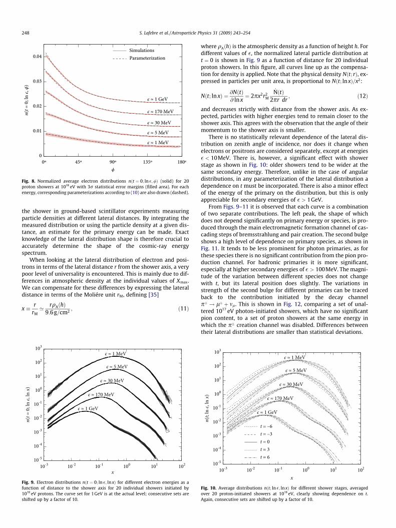
the shower in ground-based scintillator experiments measuringparticle densities at different lateral distances. By integrating themeasured distribution or using the particle density at a given dis-tance, an estimate for the primary energy can be made. Exactknowledge of the lateral distribution shape is therefore crucial toaccurately determine the shape of the cosmic-ray energyspectrum.

When looking at the lateral distribution of electron and posi-trons in terms of the lateral distance r from the shower axis, a verypoor level of universality is encountered. This is mainly due to dif-ferences in atmospheric density at the individual values of Xmax.We can compensate for these differences by expressing the lateraldistance in terms of the Moliére unit rM, defining [35]

x # rrM

’ rqA$h%9:6g=cm2 ; $11%

where qA$h% is the atmospheric density as a function of height h. Fordifferent values of !, the normalized lateral particle distribution att & 0 is shown in Fig. 9 as a function of distance for 20 individualproton showers. In this figure, all curves line up as the compensa-tion for density is applied. Note that the physical density N$t; r%, ex-pressed in particles per unit area, is proportional to N$t; ln x%=x2:

N$t; ln x% & @N$t%@ ln x

& 2px2r2M_N$t%

2pr dr; $12%

and decreases strictly with distance from the shower axis. As ex-pected, particles with higher energies tend to remain closer to theshower axis. This agrees with the observation that the angle of theirmomentum to the shower axis is smaller.

There is no statistically relevant dependence of the lateral dis-tribution on zenith angle of incidence, nor does it change whenelectrons or positrons are considered separately, except at energies! < 10MeV. There is, however, a significant effect with showerstage as shown in Fig. 10: older showers tend to be wider at thesame secondary energy. Therefore, unlike in the case of angulardistributions, in any parameterization of the lateral distribution adependence on t must be incorporated. There is also a minor effectof the energy of the primary on the distribution, but this is onlyappreciable for secondary energies of ! > 1GeV.

From Figs. 9–11 it is observed that each curve is a combinationof two separate contributions. The left peak, the shape of whichdoes not depend significantly on primary energy or species, is pro-duced through the main electromagnetic formation channel of cas-cading steps of bremsstrahlung and pair creation. The second bulgeshows a high level of dependence on primary species, as shown inFig. 11. It tends to be less prominent for photon primaries, as forthese species there is no significant contribution from the pion pro-duction channel. For hadronic primaries it is more significant,especially at higher secondary energies of ! > 100MeV. The magni-tude of the variation between different species does not changewith t, but its lateral position does slightly. The variations instrength of the second bulge for different primaries can be tracedback to the contribution initiated by the decay channelp" ! l" ' ml. This is shown in Fig. 12, comparing a set of unal-tered 1017 eV photon-initiated showers, which have no significantpion content, to a set of proton showers at the same energy inwhich the p" creation channel was disabled. Differences betweentheir lateral distributions are smaller than statistical deviations.

Fig. 10. Average distributions n$t; ln !; ln x% for different shower stages, averagedover 20 proton-initiated showers at 1018 eV, clearly showing dependence on t.Again, consecutive sets are shifted up by a factor of 10.

Fig. 8. Normalized average electron distributions n$t & 0; ln !;/% (solid) for 20proton showers at 1018 eV with 3r statistical error margins (filled area). For eachenergy, corresponding parameterizations according to (10) are also drawn (dashed).

Fig. 9. Electron distributions n$t & 0; ln !; ln x% for different electron energies as afunction of distance to the shower axis for 20 individual showers initiated by1018 eV protons. The curve set for 1GeV is at the actual level; consecutive sets areshifted up by a factor of 10.


This observation raises the question whether one could use thisdifference in lateral distribution to differentiate between primarieson an individual shower basis by their lateral distribution, inde-pendently of measurements of primary energy or depth of showermaximum. This would be a difficult task. First of all, appreciabledifference in density only occurs at high energies and at some dis-tance, implying that the total electron density in the region of sen-sitivity would be very small. Additionally, the effect does notappear at the same distance for different electron energies. Thismakes the feature less pronounced when an integrated energyspectrum is measured.

Traditionally, the integral lateral electron distribution is de-scribed by an approximation of the analytical calculation of the lat-eral distribution in electromagnetic cascades, the Nishimura–Kamata–Greisen (NKG) function [36,37]. The integral lateral distri-bution for our simulated set of showers n$t; ln x% / x2qnkg is repro-duced well by a parameterization of this form, provided that weallow the parameters to be varied somewhat. Let us define

n$t; ln x% & C2xf0 $x1 ' x%f1 $13%

as parameterization. In the original definition, described in terms ofshower age s, we have f0 & s; f1 & s! 4:5, and x1 & 1. Our simulatedlateral spectra closely follow the values f0 & 0:0238t ' 1:069; f1 &0:0238t ! 2:918, and x1 & 0:430 to an excellent level for 10!3 <x < 10.

To reproduce the main bulge in the energy-dependent lateralelectron distributions, we propose a slightly different function.The second bulge will be ignored here since it is much lower thanthe primary bulge, and its relative height depends heavily on pri-mary species as mentioned earlier. The proposed parameterizationis the same as (13):

n$t; ln !; ln x% & C 02x

f00 $x01 ' x%f01 ; $14%

mimicking the behaviour of the NKG function, but now also varyingthe parameters with !. Appendix A.4 explains the values of x0i and f0i.As an example of the fit, Fig. 13 compares the parameterization tothe average distribution for proton showers at their maximum.The proposed parameters adequately reproduce the main bulge ofthe lateral distribution in the energy range of 1MeV < ! < 1GeVfor distances x > 2 , !3 and evolution stages !6 < t < 9.

Neglecting the second bulge results in a slightly overestimatedoverall value for the normalization. The disregarded tail only con-stitutes a minor fraction of the total number of particles, however,especially at high energies. This fact becomes even more evident ifone considers that the actual distribution is obtained by dividingby x2.

The position of the break xc, the distance of the highest peak inthe distribution, is plotted in Fig. 14 for various shower stages for20 averaged showers. The theoretical break distance from the ori-ginal Nishimura–Kamata–Greisen distribution at the shower max-imum, which is an integral distribution over all electron energies,is also plotted as a horizontal line. At lower energies, the two arein good agreement as expected.

8. Delay time distribution

For radio geosynchrotron measurements the arrival time ofcharged particles is a vital quantity, because it determines thethickness of the layer of particles that form the air shower. This

Fig. 11. Average distributions n$t & 0; ln !; ln x% for different primaries, averagedover 20 showers at 1018 eV. Again, consecutive sets are shifted up by a factor of 10.Note the dependence on species of the bulge on the right.

Fig. 12. Comparison of average distributions n$t & 0; ln !; ln x% at 1017 eV for 20standard photon showers to 20 proton showers in which p" decay was disabled.Again, consecutive sets are shifted up by a factor of 10.

Fig. 13. Normalized average electron distributions n$t & 0; ln !; ln x% (solid) for 20proton showers at 1018 eV with 3r statistical error margins (filled area). For eachenergy, corresponding parameterizations according to (14) are also drawn (dashed).Consecutive sets are again shifted up by a factor of 10.


thickness in turn defines the maximum frequency up to which theresulting radio signal is coherent [33,38], which influences thestrength of the radio signal on the ground.

Let us define the delay time Dt of a particle as the time lag withrespect to an imaginary particle continuing on the cosmic-ray pri-mary’s trajectory with the speed of light in vacuum from the firstinteraction point. In the distribution of these time lags we mustagain compensate for differences in Moliére radius to obtain a uni-versal description by introducing the variable

s # cDtrM

; $15%

where c is the speed of light in vacuum. At sea level, s & 1 corre-sponds to a time delay of 0.26 ls. The normalized delay time distri-bution at the shower maximum for different values of ! is shown inFig. 15 as a function of delay time for 20 individual proton showers.Note the striking resemblance of the time lag distribution to the lat-eral particle distribution (cf. Fig. 9). This similarity is a direct resultof the non-planar shape of the shower front as discussed in the next

section. Therefore, every characteristic in the lateral distributionwill have an equivalent in the time lag distribution.

The dependencies on primary energy, species, and angle of inci-dence closely follow those observed in the lateral distributions inevery aspect. This includes the behaviour of the second bulge withprimary species, as shown in Fig. 16. Pion-decay-initiated electronsand positrons are again responsible for the emergence of this peak.

Given the similarity between the lateral and delay time distri-butions, we use a function of the same form as (14) to parameter-ize this distribution:

n$t; ln !; ln s% & C3sf000 $s1 ' s%f

001 : $16%

Appendix A.5 explains the values of si and f00i . Fig. 17 compares theparameterization above to the average distribution for protonshowers at their maximum. Again, only the main peak was includedin defining the fit parameters, causing the resulting parameterizedshape to underestimate the number of particles at long delay times.

Fig. 14. Cutoff distance xc as a function of secondary energy at different showerstages. The energy-independent overall break distance obtained from the NKG

function is also plotted (horizontal line).

Fig. 15. Electron distributions n$t & 0; ln !; ln s% for different electron energies as afunction of delay time for 20 individual showers initiated by 1019eV protons. Thecurve set for 1GeV is at the actual level; consecutive sets are shifted up by a factorof 10.

Fig. 16. Average distributions n$t & 0; ln !; lns% for different primaries, averagedover 20 showers at 1019 eV. Consecutive sets are again shifted up by a factor of 10.Note the species-dependent bulge on the right as in Fig. 11.

Fig. 17. Normalizsed average electron distributions n$t & 0; ln !; lns% (solid) for 20proton showers at 1019 eV with 3r statistical error margins (filled area). For eachenergy, corresponding parameterizations according to (16) are also drawn (dashed).Consecutive sets are again shifted up by a factor of 10.


9. Shape of the shower front

The similarity between the lateral and delay time distributionsof electrons and positrons as investigated in the previous sectionsis the result of the spatial extent of an air shower at a given time. Itmakes sense, therefore, to investigate the physical shape of theshower front by looking at the dependence of the distribution onlateral and delay time simultaneously. In order to keep the analysispracticable, we will abandon energy dependence here in our study.

For 20 proton shower simulations at 1019 eV, the shower frontshape at the shower maximum is displayed in Fig. 18 at differentdistances from the shower core. The distribution shown isn$t; ln x; s%, and each curve is scaled to a similar level for easiercomparison of the distributions. Though the low number of parti-cles leads to larger fluctuations of the distributions at high dis-tances, the behaviour clearly does not change significantly forx > 3.

No significant dependence of the shower front shape on inci-dence angle was found for x < 15, nor is there any change with pri-mary energy. There are fluctuations with evolution stage, howeverthe time lag decreases by a constant fraction which depends on theshower stage. As the shower evolves, the entire distribution shiftsto the left. This effect, shown in Fig. 19, can be explained from theincreasing spatial structure of the shower with age, not unlike thecase of an expanding spherical shell. We shall see further on thatthe analogy is not entirely legitimate, but the shift does allowone to estimate Xmax from the arrival times of the particles. We alsofound a non-negligible dependence of the delay time on primaryspecies, which is comparable in nature to the effect of evolutionstage, as shown in Fig. 20. The dependence of the distribution onboth species and evolution stage can be removed almost entirelyfor distances of 0:03 < x < 15 by applying a simple exponentialshift in s. Additionally, the distributions shown are integrated overenergy. Therefore, the shape of the distribution changes when elec-trons or positrons are considered separately, since their energy dis-tribution is different as well.

The particle distribution at a certain distance from the showercore as a function of arrival time is usually parameterized as agamma probability density function [39,40], given by

n$t; ln x; s% / exp(a0 ln s! a1s): $17%

We have found that such a parameterization does not follow oursimulated distributions very well. Its slope is too gentle at short de-

lay times and too steep at long time lags. Here, we use the betterrepresentation

n$t; ln x; s% & C4 exp(a0 lns0 ! a1ln2s0); $18%

which allows for a more gradual slope on the right side of the curve.The modified time lag s0 takes into account the exponential shiftmentioned earlier, and is defined as

s0 # se!btt!bs ; $19%

where bt and bs are corrections for shower evolution stage and pri-mary species, respectively. The values of the parametersa0$x%; a1$x%;bt, and bs are explained in Appendix A.6. The parameterbt can be seen as a scale width for the expansion of the shower frontas it develops. Note that the integral lateral distribution as param-eterized in (13) is needed to obtain actual particle numbers via

N$t; ln x; s% & N$t%n$t; ln x%n$t; ln x; s%; $20%

using the identities in (4).We may exploit the necessity of the parameter bs in our

description of the shower front shape to determine the primaryFig. 18. Electron distributions n$t & 0; ln x; s% as a function of particle time lag for20 individual showers initiated by 1019 eV protons.

Fig. 19. Average distributions n$t; ln x; s% for different evolution stages, averagedover 20 proton-initiated showers at 1019 eV.

Fig. 20. Average distributions n$t & 0; ln x; s% for different primary species, aver-aged over 20 proton-initiated showers at 1019 eV.


species if the value of Xmax is known. To distinguish proton fromphoton showers in this manner, the required resolution in showerstage is dt < bs=bt ’ 0:52, assuming perfect timing and distanceinformation. This corresponds to an error in Xmax of 19g=cm2. Toseparate proton from iron showers, the maximum error is reducedto 11g=cm2. Unfortunately, these figures are similar to or smallerthan statistical fluctuations in individual showers or systematicuncertainties in the atmospheric density due to weather influences[41,42]. This makes it very difficult to take advantage of this intrin-sic difference.

An example of the fit of (18) at t & 0 is shown in Fig. 21. For dis-tances xJ0:8, the fit describes the simulations very accurately.Equivalence is partially lost at small distances, because the shapeof the distribution becomes more complicated closer to the showercore. Even there, however, the resulting shape is reasonably accu-rate down to x ’ 0:04. Also plotted are best-fit gamma probabilitydensity functions according to (17) for each distance, which are oflower quality than the parameterization used here, especially closeto the core.

For a certain distance from the shower core, we define the timelag sc as the time lag where the particle density is at its maximum,corresponding to the peaks of the curves shown earlier in this sec-tion. Its value at the shower maximum is shown in Fig. 22 as afunction of X for the reference simulation set. The two straightlines represent fits of the form sc & Axk to the part before (dashed)and after the break (dotted) as shown in the plot. The time lag ofthe maximum particle density can be parameterized as

sc &$0:044! 0:00170t%x1:79!0:0056t x < x0;$0:028! 0:00049t%x1:46!0:0007t x > x0;

(

$21%

where the value for x0 follows from continuity. One could employthis function to estimate the value of Xmax, though the accuracyattainable in this way is probably much lower than using fluores-cence measurements.

In experiments, the shower front is sometimes approximated asa spherical shell [43]. How do the simulated distributions compareto such a hypothetical shape? Close to the shower core, wherer - R (with R ’ 50 the supposed curvature radius in Moliére units)we expect k & 2 and R & A!1. Going out, the slope should then de-crease slowly as X approaches the presumed curvature radius.

This spherical shape does not correspond to the situation in oursimulations. In the innermost region the exponent gives consis-tently smaller values of k ’ 1:79. Further out, there is an abrupttransition around x ’ 0:3, and the final exponent is k ’ 1:45.

10. Conclusion

In this work, we have presented a framework for the accuratedescription of electron–positron distributions in extensive airshowers. To characterize the longitudinal evolution of the airshower, the concept of slant depth relative to the shower maxi-mum is used.

Using the CORSIKA code, we have built a library of simulationsof air showers. Analysis of this library shows that, to a largeextent, extensive air showers show universal behaviour at very-high-energy, making the distributions in them dependent on onlytwo parameters: the atmospheric depth Xmax where the numberof particles in the air shower peaks and the total number of parti-cles Nmax present in the shower at this depth. The entire structureof the shower follows directly from these two values.

We have found some exceptions to the universality hypothesisin the spatial distribution of particles. Theoretically, these non-uni-versal features can be employed to distinguish primaries on ashower-to-shower basis. In real experiments, however, this wouldbe a difficult task because the effect either amounts to only a fewpercent, or its behaviour can be mistaken for variations in showerstage.

To support the simulation of secondary radiation effects fromextensive air showers, we have provided two-dimensional param-eterizations to describe the electron–positron content in terms ofstage vs. energy and stage vs. lateral distance. We have also sup-plied three-dimensional representations of the electron contentin terms of stage vs. energy vs. vertical momentum angle, stagevs. energy vs. horizontal momentum angle, stage vs. energy vs. lat-eral distance close to the shower core, and stage vs. lateral distancevs. arrival time.

Though these parameterizations provide accurate descriptionsof the electron–positron distributions in air showers, the authorswould like to mention that there are no theoretical grounds formost of the functional representations suggested in this work.Their choice is justified only by the flexibility of the functions toaccurately reproduce the simulated distributions as fit functionswith a small number of parameters. Additionally, the parameter-izations provided are based on simulations with a single interac-

Fig. 21. Average electron distributions n$t & 0; ln x; s% (solid) for the reference setwith 3r statistical error margins (filled area). For each distance, correspondingparameterizations according to (18) are drawn as well (dashed). Best-fit C-pdf arealso plotted (dotted).

Fig. 22. Maximum density sc as a function of lateral distance X at the showermaximum. Also shown are curves for x < x0 (dashed) and x > x0 (dotted) accordingto the parameterization in (21).


tion model only. Though no significant changes are expected in thegeneral behaviour, the parameters listed will likely change when adifferent model is employed.

When used together with a longitudinal description for the totalnumber of particles, accurate characterizations of any large airshower in terms of the relevant quantities can be calculated. Thesemay be used for realistic electron–positron distributions withoutthe need for extensive simulations and could be useful in calcula-tions of fluorescence, radio or air Cherenkov signals from very-high-energy cosmic-ray air showers.

Acknowledgements

The authors wish to express their gratitude to Markus Rissewhose help was indispensable in setting up the simulations, andto an anonymous reviewer for useful suggestions to improve themanuscript. One of the authors, R.E., acknowledges fruitful discus-sions with Paolo Lipari on the subject of shower universality. Thiswork is part of the research programme of the ‘Stich-ting voor Fun-da-men-teel Onder-zoek der Ma-terie (FOM)’, which is financiallysupported by the ‘Neder-landse Orga-ni-sa-tie voor Weten-schap-pe-lijk Onder-zoek (NWO)’. T. Huege was supported by GrantNo. VH-NG-413 of the Helmholtz Association.

Appendix A. Fit parameters

This appendix explains in detail the various parameters used inthe functional parameterizations throughout this paper. All ofthese were obtained by performing minimization sequences usinga non-linear least-squares Marquardt–Levenberg algorithm.

A.1. Energy spectrum

The parameters in the energy spectrum distribution function asput forward in (6) were chosen to match those advocated in Ner-ling et al. [10]. A good description is obtained with the parameterslisted in Table 1. The constants in !1 and !2 are in MeV; the con-stant A0 is provided here for all three cases to obtain charge excessvalues; the overall parameter A1 in the table follows directly fromnormalization constraints.

A.2. Vertical angular spectrum

The distribution of the particles’ momentum angle away fromthe shower axis can be parameterized accurately as

n$t; ln !;X% & C0 eb1ha1! "!1=r ' eb2ha2

! "!1=rh i!r: $8%

For secondary energies 1MeV < ! < 10GeV and angles up to 60",the curves are described well for n$t; ln !;X% > 10!4 by setting theparameters in the equations above, using nine free parameters, to

b1 & !3:73' 0:92!0:210;b2 & 32:9! 4:84 ln !;a1 & !0:399; $A:1%a2 & !8:36' 0:440 ln !:

The constant r is a parameter describing the smoothness of thetransition of the distribution function from the first term of impor-tance near the shower axis to the second term being relevant fur-ther away and was set to r & 3. The overall factor C0 follows fromthe normalization condition.

A.3. Horizontal angular spectrum

The horizontal distribution of momentum is given by

n$t; ln !;/% & C1(1' exp$k0 ! k1/! k2/2%); $10%

where optimal agreement is reached in the intervals1 MeV < ! < 10GeV and !6 < t < 9 by setting

k0 & 0:329! 0:0174t ' 0:669 ln !! 0:0474ln2!;

k1 & 8:10 , 10!3 ' 2:79 , 10!3 ln !; $A:2%

k2 & 1:10 , 10!4 ! 1:14 , 10!5 ln !

with all energies in MeV. There were eight free parameters in totalin the fit. The value of C1 follows directly from the normalization in(5).

A.4. Lateral distribution

The NKG-like function to describe the primary peak in the lateraldistribution is defined as

n$t; ln !; ln x% & C 02x

f00 $x01 ' x%f01 : $14%

The fit was performed in the interval 1MeV < ! < 10GeV, with theadditional condition that x < 5xc in order to discard the second, spe-cies-dependent peak. Optimal correlation is obtained by using theparameters

x01 & 0:859! 0:0461ln2!' 0:00428ln3!;ft & 0:0263t;

f00 & ft ' 1:34' 0:160 ln !! 0:0404ln2!' 0:00276ln3!; $A:3%f01 & ft ! 4:33

with nine free parameters in total. The value of ! is always ex-pressed in MeV. Again, the value of C0

2 follows directly from normal-ization constraints and will not be discussed here.

A.5. Delay time distribution

The fit function to describe the primary peak in the delay timedistribution is identical to that of the lateral distribution,

n$t; ln !; ln s% & C3sf000 $s1 ' s%f

001 $16%

and was performed at energies 1MeV < ! < 10GeV, discarding thesecond peak. Best-fit parameters are

s1 & exp(!2:71' 0:0823 ln !! 0:114ln2!);f000 & 1:70' 0:160t ! 0:142 ln !; $A:4%f001 & !3:21

with ! in MeV, using seven free parameters in total. The constant C3

again follows from normalization.

Table 1Parameter values for the energy spectrum in (6) for species of electrons, positrons, and the sum of electrons and positrons.

A0 !1 !2 c1 c2Electrons 0:485A1 exp$0:183t ! 8:17t2 , 10!4% 3:22! 0:0068t 106! 1:00t 1 1' 0:0372tPositrons 0:516A1 exp$0:201t ! 5:42t2 , 10!4% 4:36! 0:0663t 143! 0:15t 2 1' 0:0374tTotal A1 exp$0:191t ! 6:91t2 , 10!4% 5:64! 0:0663t 123! 0:70t 1 1' 0:0374t


A.6. Shape of the shower front

The shape of the shower front is parameterized as

n$t; ln x; s% & C4 exp(a0 log s0 ! a1log2s0); $18%

inspired by the gamma probability distribution, with

s0 # se!btt!bs : $19%

The following parameters give optimal results:

a0 & !6:04' 0:707log2x' 0:210log3x

! 0:0215log4x! 0:00269log5x; $A:5%

a1 & 0:855' 0:335 log x' 0:0387log2x! 0:00662log3x:

The value for bt is fixed at bt & 0:20, while bs depends on the pri-mary species:

bs & !0:062 for iron nuclei;bs # 0 for protons; $A:6%bs & 0:103 for photons:

These parameters are valid for distances of 0:4 < x < 102 and10!4 < s0 < 10.

References

[1] R.M. Baltrusaitis, R. Cady, G.L. Cassiday, et al., Nucl. Instr. Meth. A 240 (1985)410.

[2] H. Falcke et al., Nature 435 (2005) 313.[3] B. Rossi, K. Greisen, Rev. Mod. Phys. 13 (1941) 240.[4] J. Nishimura, Handbuch Phys. (46/2) (1965) 1.[5] A.M. Hillas, J. Phys. G Nucl. Phys. 8 (1982) 1461.[6] M. Giller, A. Kacperczyk, J. Malinowski, W. Tkaczyk, G. Wieczorek, J. Phys. G 31

(2005) 947.[7] M. Giller, H. Stojek, G. Wieczorek, International Journal of Modern Physics A 20

(2005) 6821.[8] D. Góra, R. Engel, D. Heck, et al., Astropart. Phys. 24 (2006) 484.[9] A.S. Chou et al., in: Proc. 29th Int. Cosmic Ray Conf., vol. 7, 2005, p. 319.

[10] F. Nerling, J. Blümer, R. Engel, M. Risse, Astropart. Phys. 24 (2006) 421.[11] P. Billoir, C. Roucelle, J.-C. Hamilton, 2007. ArXiv Astrophysics e-prints, astro-

ph/0701583.[12] F. Schmidt, M. Ave, L. Cazon, A. Chou, Astropart. Phys. 29 (2008) 355.[13] D. Heck, J. Knapp, et al., CORSIKA: A Monte Carlo Code to Simulate Extensive

Air Showers, Tech. Rep. 6019, Forschungszentrum Karlsruhe, 1998.[14] S. Ostapchenko, Phys. Rev. D 74 (2006) 014026.[15] S. Ostapchenko, Phys. Lett. B 636 (2006) 40.[16] S.A. Bass, M. Belkacem, M. Bleicher, et al., Prog. Part. Nucl. Phys. 41 (1998) 225.[17] M. Bleicher, E. Zabrodin, C. Spieles, et al., J. Phys. G 25 (1999) 1859.[18] W. Nelson, H. Hirayama, D. Rogers, The EGS4 Code System, Tech. Rep. 265,

Stanfod Linear Accelerator Center, 1985.[19] Pierre Auger Collaboration, M. Kobal, Astropart. Phys. 15 (2001) 259.[20] M. Risse, D. Heck, J. Knapp, in: Proc. 27th Int. Cosmic Ray Conf., vol. 2, 2001,

522.[21] National Aeronautics and Space Administration (NASA), US Standard

Atmosphere, Tech. Rep. NASA-TM-X-74335, 1976.[22] J. Knapp, D. Heck, Tech. Rep. 5196B, Kernforschungszentrum Karlsruhe, 1993.[23] R. Ulrich, 2007. <http://www-ik.fzk.de/~rulrich/coast/>.[24] T. Erber, Rev. Mod. Phys. 38 (1966) 626.[25] B. McBreen, C.J. Lambert, Phys. Rev. D 24 (1981) 2536.[26] S. Lafebre, T. Huege, H. Falcke, J. Kuijpers, in: Proc. 30th Int. Cosmic Ray Conf.,

2007.[27] P. Lipari, 2008. ArXiv Astrophysics e-prints, 0809.0190.[28] Müller, Diploma Thesis, Univ. Karlsruhe, 2008.[29] K. Greisen, Ann. Rev. Nucl. Part Sci. 10 (1960) 63.[30] T.K. Gaisser, A.M. Hillas, in: Proc. 15th Int. Cosmic Ray Conf., 1978, pp. 353–

357.[31] T. Abu-Zayyad, K. Belov, D.J. Bird, et al., Astropart. Phys. 16 (2001) 1.[32] C.L. Pryke, Astropart. Phys. 14 (2001) 319.[33] T. Huege, H. Falcke, Astron. Astrophys. 412 (2003) 19.[34] J.W. Elbert, T. Stanev, S. Torii, in: Proc. 18th Int. Cosmic Ray Conf., vol. 6, 1983,

pp. 227–230.[35] M.T. Dova, L.N. Epele, A.G. Mariazzi, Astropart. Phys. 18 (2003) 351.[36] K. Kamata, J. Nishimura, Progr. Theor. Phys. Suppl. 6 (1958) 93.[37] K. Greisen, in: Proc. 9th Int. Cosmic Ray Conf., vol. 1, 1965, p. 609.[38] O. Scholten, K. Werner, F. Rusydi, Astropart. Phys. 29 (2008) 94.[39] C.P. Woidneck, E. Bohm, J. Phys. A Math. Gen. 8 (1975) 997.[40] G. Agnetta, M. Ambrosio, C. Aramo, et al., Astropart. Phys. 6 (1997) 301.[41] B. Keilhauer, J. Blümer, R. Engel, H.O. Klages, M. Risse, Astropart. Phys. 22

(2004) 249.[42] B. Wilczynska, D. Góra, P. Homola, et al., Astropart. Phys. 25 (2006) 106.[43] B.R. Dawson, C.L. Pryke, in: Proc. 25th Int. Cosmic Ray Conf., vol. 5, 1997, p.

213.


http://www-ik.fzk.de/~rulrich/coast/

universality of electron–positron distributions in...

Documents