universidad politécnica de madrid - archivo digital upmoa.upm.es/37208/1/xin_chen.pdf ·...
TRANSCRIPT

Universidad Politécnica de MadridEscuela Técnica Superior de Ingenieros Aeronáuticos
Low Work-Function Thermionic Emission
and Orbital-Motion-Limited Ion Collection
at Bare-Tether Cathodic Contact
Tesis Doctoral
Xin Chen
Madrid, Junio 2015


Departamento de Física Aplicada a la Ingeniería Aeronáutica y Naval
Escuela Técnica Superior de Ingenieros Aeronáuticos
Low Work-Function Thermionic Emission
and Orbital-Motion-Limited Ion Collection
at Bare-Tether Cathodic Contact
Ph.D. Thesis Dissertation
Xin ChenBs in Electrical Engineering
MSc in Aerospace Engineering
Proposed and supervised by
Juan Ramón Sanmartín LosadaFull Professor in Aerospace Engineering
Gonzalo Sánchez-ArriagaProfessor in Aerospace Engineering
Madrid, June 2015

Tribunal nombrado por el Sr. Rector Magfco. de la Universidad Politécnica de
Madrid, el día ...... de ............... de 2015.
Presidente: Dr. Francisco Javier Sanz Recio
Vocal: Dr. Carlos Hidalgo
Vocal: Dr. Alain Hilgers
Vocal: Dr. Eduardo Ahedo
Secretario: Dr. Jose Javier Honrubia Checa
Suplente: Dr. Mario Merino Martínez
Suplente: Dr. Juan Arturo Alonso De Pablo
Realizado el acto de defensa y lectura de la Tesis el día 1 de julio de 2015 en la
E.T.S.I. Aeronáuticos.
Calificación ...................................................
EL PRESIDENTE LOS VOCALES
EL SECRETARIO
iii


It was harder to work out that there
was a question than to think of the
answer.
Richard Dawkins
The Selfish Gene
v


Abstract
An electrodynamic tether operates on electromagnetic principles and exchanges mo-
mentum through the planetary magnetosphere, by continuously interacting with the
ionosphere. It is a reliable passive subsystem to deorbit spent rocket stages and satel-
lites at its end of mission, mitigating the growth of orbital debris. A tether left bare
of insulation collects electrons by its own uninsulated and positively biased segment
with kilometer range, while electrons are emitted by a low-impedance active device at
the cathodic end, such as a hollow cathode, to emit the full electron current.
In the absence of an active cathodic device, the current flowing along an orbiting
bare tether vanishes at both ends and the tether is said to be electrically floating. For
negligible thermionic emission and orbital-motion-limited (OML) collection through-
out the entire tether (electron/ion collection at anodic/cathodic segment, respectively),
the anodic-to-cathodic length ratio is very small due to ions being much heavier, which
results in low average current and Lorentz drag.
The electride C12A7 : e−, which might present a possible work function as low as
W = 0.6 eV and moderately high temperature stability, has been proposed as coating
for floating bare tethers. Thermionic emission along a thus coated cathodic segment,
under heating in space operation, can be more efficient than ion collection and, in
the simplest drag mode, may eliminate the need for an active cathodic device and its
corresponding gas-feed requirements and power subsystem, which would result in a
truly “propellant-less” tether system.
With this low-W coating, each elemental segment on the cathodic segment of a
kilometers-long floating bare-tether would emit current as if it were part of a hot cylin-
drical probe uniformly polarized at the local tether bias, under 2D probe conditions
that are also applied to the anodic-segment analysis. In the presence of emission, emit-
ted electrons result in negative space charge, which decreases the electric field that
accelerates them outwards, or even reverses it, decelerating electrons near the emit-
ting probe. A double sheath would be established with electrons being emitted from
the probe and ions coming from the ambient plasma. The thermionic current density,
varying along the cathodic segment, might follow two distinct laws under different con-
vii

ditions: i) space-charge-limited (SCL) emission or ii) full Richardson-Dushman (RDS)
emission.
A preliminary study on the SCL current in front of an emissive probe is presented
using the orbital-motion-limited (OML) ion-collection sheath and Langmuir’s SCL
electron current between cylindrical electrodes. A detailed calculation of current and
bias profiles along the entire tether length is carried out with ohmic effects considered
and the transition from SCL to full RDS emission is included. Analysis shows that
in the simplest drag mode, under typical orbital and tether conditions, thermionic
emission provides efficient cathodic contact and leads to a short cathodic section.
In the previous analysis, both the transition between SCL and RDS emission and
the current law for SCL condition have used a very simple model. To continue, con-
sidering an isotropic, unmagnetized, colissionless plasma and a stationary sheath, the
probe-plasma contact is studied in detail for a negatively biased probe with thermionic
emission. The possible trapped particles are ignored and this study includes both semi-
analytical solutions using asymptotic analysis and complete numerical solutions.
Under conditions of i) high bias, ii) R = Rmax for ion OML collection validity, and
iii) monotonic potential, a self-consistent asymptotic analysis is carried out for the
complex plasma structure involving all three charge species (plasma electrons and ions,
and emitted electrons) and four distinct spatial regions using orbital motion theories
and kinetic modeling of the species. Although emitted electrons present negligible
space charge far away from the probe, their effect cannot be neglected in the global
analysis for the sheath structure and two thin layers in between the sheath and the
quasineutral region. The parametric conditions for the current to be space-charge-
limited are obtained. It is found that thermionic emission increases the range of probe
radius for OML validity and is greatly more effective than ion collection for cathodic
contact of tethers.
In the numerical code, the orbital motions of all three species are modeled for both
monotonic and non-monotonic potential, and for any probe radius R (within or beyond
OML regime for ion collection). Taking advantage of two constants of motion (energy
and angular momentum), the Poisson-Vlasov equation is described by an integro dif-
ferential equation, which is discretized using finite difference method. The non-linear
algebraic equations are solved using a parallel implementation of the Newton-Raphson
method. The results, which show good agreement with the analytical results, provide
the results for thermionic current, the sheath structure, and the electrostatic potential.
viii
Resumen
Una amarra electrodinámica (electrodynamic tether) opera sobre principios electro-
magnéticos intercambiando momento con la magnetosfera planetaria e interactuando
con su ionosfera. Es un subsistema pasivo fiable para desorbitar etapas de cohetes
agotadas y satélites al final de su misión, mitigando el crecimiento de la basura espa-
cial. Una amarra sin aislamiento captura electrones del plasma ambiente a lo largo
de su segmento polarizado positivamente, el cual puede alcanzar varios kilómetros de
longitud, mientras que emite electrones de vuelta al plasma mediante un contactor de
plasma activo de baja impedancia en su extremo catódico, tal como un cátodo hueco
(hollow cathode).
En ausencia de un contactor catódico activo, la corriente que circula por una
amarra desnuda en órbita es nula en ambos extremos de la amarra y se dice que ésta
está flotando eléctricamente. Para emisión termoiónica despreciable y captura de cor-
riente en condiciones limitadas por movimiento orbital (orbital-motion-limited, OML),
el cociente entre las longitudes de los segmentos anódico y catódico es muy pequeño
debido a la disparidad de masas entre iones y electrones. Tal modo de operación re-
sulta en una corriente media y fuerza de Lorentz bajas en la amarra, la cual es poco
eficiente como dispositivo para desorbitar.
El electride C12A7 : e−, que podría presentar una función de trabajo (work func-
tion) tan baja como W = 0.6 eV y un comportamiento estable a temperaturas rela-
tivamente altas, ha sido propuesto como recubrimiento para amarras desnudas. La
emisión termoiónica a lo largo de un segmento así recubierto y bajo el calentamiento
de la operación espacial, puede ser más eficiente que la captura iónica. En el modo más
simple de fuerza de frenado, podría eliminar la necesidad de un contactor catódico ac-
tivo y su correspondientes requisitos de alimentación de gas y subsistema de potencia,
lo que resultaría en un sistema real de amarra “sin combustible”.
Con este recubrimiento de bajo W , cada segmento elemental del segmento catódico
de una amarra desnuda de kilómetros de longitud emitiría corriente como si fuese
parte de una sonda cilíndrica, caliente y uniformemente polarizada al potencial local
de la amarra. La operación es similar a la de una sonda de Langmuir 2D tanto
ix

en los segmentos catódico como anódico. Sin embargo, en presencia de emisión, los
electrones emitidos resultan en carga espacial (space charge) negativa, la cual reduce
el campo eléctrico que los acelera hacia fuera, o incluso puede desacelerarlos y hacerlos
volver a la sonda. Se forma una doble vainas (double sheath) estable con electrones
emitidos desde la sonda e iones provenientes del plasma ambiente. La densidad de
corriente termoiónica, variando a lo largo del segmento catódico, podría seguir dos
leyes distintas bajo diferentes condiciones: (i) la ley de corriente limitada por la carga
espacial (space-charge-limited, SCL) o (ii) la ley de Richardson-Dushman (RDS).
Se presenta un estudio preliminar sobre la corriente SCL frente a una sonda emisora
usando la teoría de vainas (sheath) formada por la captura iónica en condiciones
OML, y la corriente electrónica SCL entre los electrodos cilíndricos según Langmuir.
El modelo, que incluye efectos óhmicos y el efecto de transición de emisión SCL a
emisión RDS, proporciona los perfiles de corriente y potencial a lo largo de la longitud
completa de la amarra. El análisis muestra que en el modo más simple de fuerza
de frenado, bajo condiciones orbitales y de amarras típicas, la emisión termoiónica
proporciona un contacto catódico eficiente y resulta en una sección catódica pequeña.
En el análisis anterior, tanto la transición de emisión SCL a RD como la propia
ley de emisión SCL consiste en un modelo muy simplificado. Por ello, a continuación
se ha estudiado con detalle la solución de vaina estacionaria de una sonda con emisión
termoiónica polarizada negativamente respecto a un plasma isotrópico, no colisional y
sin campo magnético. La existencia de posibles partículas atrapadas ha sido ignorada
y el estudio incluye tanto un estudio semi-analítico mediante técnica asintóticas como
soluciones numéricas completas del problema.
Bajo las tres condiciones (i) alto potencial, (ii) R = Rmax para la validez de la
captura iónica OML, y (iii) potencial monotónico, se desarrolla un análisis asintótico
auto-consistente para la estructura de plasma compleja que contiene las tres especies de
cargas (electrones e iones del plasma, electrones emitidos), y cuatro regiones espaciales
distintas, utilizando teorías de movimiento orbital y modelos cinéticos de las especies.
Aunque los electrones emitidos presentan carga espacial despreciable muy lejos de la
sonda, su efecto no se puede despreciar en el análisis global de la estructura de la vaina
y de dos capas finas entre la vaina y la región cuasi-neutra. El análisis proporciona
las condiciones paramétricas para que la corriente sea SCL. También muestra que la
emisión termoiónica aumenta el radio máximo de la sonda para operar dentro del
régimen OML y que la emisión de electrones es mucho más eficiente que la captura
iónica para el segmento catódico de la amarra.
x

En el código numérico, los movimientos orbitales de las tres especies son modelados
para potenciales tanto monotónico como no-monotónico, y sonda de radio R arbitrario
(dentro o más allá del régimen de OML para la captura iónica). Aprovechando la exis-
tencia de dos invariante, el sistema de ecuaciones Poisson-Vlasov se escribe como una
ecuación integro-diferencial, la cual se discretiza mediante un método de diferencias
finitas. El sistema de ecuaciones algebraicas no lineal resultante se ha resuelto de con
un método Newton-Raphson paralelizado. Los resultados, comparados satisfactoria-
mente con el análisis analítico, proporcionan la emisión de corriente y la estructura
del plasma y del potencial electrostático.
xi


Acknowledgements
First of all, I would not have been able to finish this thesis without the uncondi-
tional support, uncountable love and unlimited patience of my adorable fiancé, Julien
Peyrard. With his out-of-nowhere eternal happiness and positive attitude, he makes
me smile every day. Without all these, I would not have been able to concentrate on
my research and keep in good spirits.
I am in deepest gratitude to my thesis advisor Professor Juan R. Sanmartín for his
valuable teachings, patience, and dedication in guiding me through all the difficulties
encountered. He has always been there to provide a wise indication. My heartfelt
thanks for all the help and opportunities he has offered me. I also would like to thank
my co-adviser Professor Gonzalo Sánchez-Arriaga. Apart from the fruitful discussions,
I have learned from him the passion, the dedication, and the vision a young engineer
or scientist should have to continue the journey of investigation and innovation. I am
also very grateful to Professor Manuel Marínez-Sánchez and Professor Paulo Lozano
for giving me the opportunity of a three months stay at Massachusetts Institute of
Technology. Besides the knowledge and experience I gained during the stay, I have
gained the responsibility and confidence a young investigator should have to contribute
to the world.
Of course, my thanks to the members of the Committee for agreeing to review
and evaluate my work, and to Professor Manuel Marínez-Sánchez and Doctor Alain
Hilgers for carrying out an evaluation report on this dissertation and providing valuable
corrections and suggestions.
Special acknowledgement to the friends from the “Plasma y Asteroides” group,
Juancho, Hodei, Mario, Jaume and Bayajid who have shared their knowledge with me
and spent endless time satisfying my doubts. I shall not forget Isidro, Artur, Chiara,
Assal, Meijuan, Ana, Laura, Sole, Fernando, and the rest of my friends in Madrid,
who have shared these years with me, cared for me, and been there for me whenever
I needed.
At last but most important, I would like to specially thank my parents for all they
have done in these 28 years, for always being on my side, being comprehensive and
xiii

supportive, and for all the sacrifices they made through their lifetime so that I could
make is this far. Without the education and patience they have given me, I would not
be who I am, I would not have achieved what I have.
xiv

Table of contents
List of figures xix
List of tables xxiii
Nomenclature xxvii
1 INTRODUCTION 1
1.1 Background on Space Tethers . . . . . . . . . . . . . . . . . . . . . . . 1
1.2 Electrodynamic Tethers . . . . . . . . . . . . . . . . . . . . . . . . . . 4
1.3 Background on Plasma, Sheath and Probe Theory . . . . . . . . . . . . 7
1.4 Dissertation Outline . . . . . . . . . . . . . . . . . . . . . . . . . . . . 12
2 BASICS ON THE STUDY 15
2.1 Electrodynamic Tether Basics . . . . . . . . . . . . . . . . . . . . . . . 15
2.1.1 Induced Current and Lorentz Force . . . . . . . . . . . . . . . . 15
2.1.2 Current Closure Loop for An Insulated Tether . . . . . . . . . . 18
2.2 Theories of Sheath around a Probe . . . . . . . . . . . . . . . . . . . . 21
2.2.1 Distribution Function in Phase Space . . . . . . . . . . . . . . . 21
2.2.2 Poisson-Vlasov System with Stationary Electric field and with-
out Magnetic Field . . . . . . . . . . . . . . . . . . . . . . . . . 23
2.2.3 Orbital-Motion-Limited Theory . . . . . . . . . . . . . . . . . . 25
2.3 Conventional Bare Tether . . . . . . . . . . . . . . . . . . . . . . . . . 34
2.3.1 OML Electron Collection at Anodic Segment . . . . . . . . . . . 36
2.3.2 Short or Long Tether . . . . . . . . . . . . . . . . . . . . . . . . 40
2.3.3 Average Current and Drag Force . . . . . . . . . . . . . . . . . . 42
2.3.4 Non-Negligible Hollow-Cathode Drop . . . . . . . . . . . . . . . 43
3 PRELIMINARY MODEL FOR BARE THERMIONIC TETHER 45
3.1 Thermionic Emission . . . . . . . . . . . . . . . . . . . . . . . . . . . . 46

Table of contents
3.1.1 Richardson-Dushman Current . . . . . . . . . . . . . . . . . . . 46
3.1.2 The Space Charge Effect . . . . . . . . . . . . . . . . . . . . . . 48
3.2 Preliminary Model for SCL Current Collection . . . . . . . . . . . . . 52
3.3 Low Work Function Electride C12A7 : e− . . . . . . . . . . . . . . . . . 53
3.4 Preliminary Study on Bare Thermionic Tether . . . . . . . . . . . . . . 56
3.4.1 Current Closure Loop . . . . . . . . . . . . . . . . . . . . . . . 58
3.4.2 The Short Case B - C . . . . . . . . . . . . . . . . . . . . . . . 59
3.4.3 The Long Case B - B* - C . . . . . . . . . . . . . . . . . . . . . 61
3.4.4 The Short/Long Cathodic-Segment Transition . . . . . . . . . . 62
3.4.5 Discussion . . . . . . . . . . . . . . . . . . . . . . . . . . . . . . 63
4 ASYMPTOTIC ANALYSIS ON THE SHEATH 67
4.1 Electron-Emitting Cylinder . . . . . . . . . . . . . . . . . . . . . . . . 68
4.1.1 Particle Densities . . . . . . . . . . . . . . . . . . . . . . . . . . 70
4.1.2 Qualitatively Description of the Solution . . . . . . . . . . . . . 72
4.1.3 Normalization . . . . . . . . . . . . . . . . . . . . . . . . . . . . 73
4.2 Matching among the Layers . . . . . . . . . . . . . . . . . . . . . . . . 74
4.2.1 z > z0 . . . . . . . . . . . . . . . . . . . . . . . . . . . . . . . . 74
4.2.2 z1 < z < z0 . . . . . . . . . . . . . . . . . . . . . . . . . . . . . 75
4.2.3 First Transitional Layer around z1 . . . . . . . . . . . . . . . . . 77
4.2.4 Second Transitional Layer around z2 . . . . . . . . . . . . . . . 79
4.2.5 Sheath and OML Validity . . . . . . . . . . . . . . . . . . . . . 80
4.2.6 Effects of Emitted Electrons . . . . . . . . . . . . . . . . . . . 82
4.2.7 Currents . . . . . . . . . . . . . . . . . . . . . . . . . . . . . . . 85
4.3 Longitudinal Structure with Moderate Ohmic and Thermionic Effects . 86
4.3.1 Bias Profile from B to B∗ . . . . . . . . . . . . . . . . . . . . . . 87
4.3.2 Current Profile from B to C . . . . . . . . . . . . . . . . . . . . 88
4.3.3 Current Profile from A to B . . . . . . . . . . . . . . . . . . . . 89
4.3.4 Weak Ohmic-Effects Case . . . . . . . . . . . . . . . . . . . . . 89
4.3.5 The Weak Ohmic-Effects Condition . . . . . . . . . . . . . . . . 91
5 KINETIC MODELING, NON-MONOTONIC POTENTIAL AND
NUMERICAL METHODS 93
5.1 Orbital Motions of All Species . . . . . . . . . . . . . . . . . . . . . . 93
5.2 Current and Particle Density . . . . . . . . . . . . . . . . . . . . . . . 96
5.2.1 Particles from Ambient Plasma at Infinity . . . . . . . . . . . . 96
5.2.2 Particles Emitted by the Probe . . . . . . . . . . . . . . . . . . 97
xvi

Table of contents
5.3 Normalization . . . . . . . . . . . . . . . . . . . . . . . . . . . . . . . . 98
5.4 Numerical Scheme . . . . . . . . . . . . . . . . . . . . . . . . . . . . . 100
5.5 Probe Behavior as Emission is Varied . . . . . . . . . . . . . . . . . . . 101
5.5.1 Currents and Potential Profiles . . . . . . . . . . . . . . . . . . 101
5.5.2 Density Profiles and Distribution Functions . . . . . . . . . . . 103
5.6 Comparison with Analytical Results . . . . . . . . . . . . . . . . . . . . 108
5.7 Conclusion . . . . . . . . . . . . . . . . . . . . . . . . . . . . . . . . . . 108
6 CONCLUSIONS 111
6.1 Results Review . . . . . . . . . . . . . . . . . . . . . . . . . . . . . . . 111
6.2 Critical Issues of Bare Thermionic Tethers . . . . . . . . . . . . . . . . 115
References 119
xvii


List of figures
1.1 Positive ion sheaths around grid wires in a thermionic tube containing
gas. . . . . . . . . . . . . . . . . . . . . . . . . . . . . . . . . . . . . . . 8
2.1 Drag or thrust for electrodynamic tethers subjected to motional elec-
tromotive force. . . . . . . . . . . . . . . . . . . . . . . . . . . . . . . . 17
2.2 Schematic of tether potential Vt and plasma potential Vpl in the tether
frame for a standard ED tether at drag mode. . . . . . . . . . . . . . . 18
2.3 Schematic of tether potential Vt and plasma potential Vpl in the tether
frame for a standard ED tether at motor mode. . . . . . . . . . . . . . 20
2.4 Plasma electrons orbits around a positive cylindrical probe without
emission. . . . . . . . . . . . . . . . . . . . . . . . . . . . . . . . . . . . 28
2.5 Schematic of cutoff boundaries and absorption boundaries in EJ-plane. 30
2.6 Schematic of potential Φ/Φp versus R2/r2 for OML regime and OML
forbidden regime. . . . . . . . . . . . . . . . . . . . . . . . . . . . . . . 34
2.7 Schematic of current and potential variation in the tether frame for a
bare tether without thermionic emission. . . . . . . . . . . . . . . . . . 35
2.8 Tether-to-plasma bias φ(ξ) and current i(ξ) along the anodic segment,
for different values of anodic end bias φA. . . . . . . . . . . . . . . . . 39
2.9 Anodic-end bias φA and current at zero-bias point iB versus the anodic-
segment length. . . . . . . . . . . . . . . . . . . . . . . . . . . . . . . 40
2.10 Influence of ohmic effects on the potential and current of a long bare
tether (L > 4L∗) without thermionic emission. . . . . . . . . . . . . . 41
2.11 The average current iav versus the total length of a bare tether without
thermionic emission. . . . . . . . . . . . . . . . . . . . . . . . . . . . . 42
3.1 Langmuir’s experimental data on the temperature saturation current. . 48
3.2 Space charge effects between parallel planes. . . . . . . . . . . . . . . 49
xix

List of figures
3.3 Emitted current density versus temperature, for C12A7 : e− electride
and other commonly used thermionic emission materials. . . . . . . . 54
3.4 Crystal structure of low work function material 12CaO · 7Al2O3. . . . 54
3.5 Schematic of current and potential variation in the tether frame for a
thermionic bare tether in drag mode. . . . . . . . . . . . . . . . . . . . 57
3.6 Anodic bias φA, collected current iB, cathodic-to-total length ratio (ξC−ξB)/ξC , cathodic bias φC , and length-averaged current iav are plotted
against tether length ξC . . . . . . . . . . . . . . . . . . . . . . . . . . . 64
4.1 Typical potential distributions of a negatively biased probe with elec-
tron emission. . . . . . . . . . . . . . . . . . . . . . . . . . . . . . . . . 69
4.2 Schematics of potential profile Φ/Φp versus R2/r2 for given emission
with different bias values, under condition R = Rmax for ion OML
collection. . . . . . . . . . . . . . . . . . . . . . . . . . . . . . . . . . . 69
4.3 Richardson-Dushman current density and emitted particle density ver-
sus probe temperature for different work function of the emitting mate-
rial. . . . . . . . . . . . . . . . . . . . . . . . . . . . . . . . . . . . . . 70
4.4 Schematic potential profile for R = Rmax. . . . . . . . . . . . . . . . . 72
4.5 Straight lines of the z-family lines j2 = j2z (ǫ). . . . . . . . . . . . . . . . 74
4.6 The maximum radius and the derivative at the probe for θ = 4 and
several ν, for a range of Ψp, and for a negatively biased probe with
thermionic emission. . . . . . . . . . . . . . . . . . . . . . . . . . . . . 82
4.7 Ψ0, Ψ1, z21/Ψp and z2
2/Ψp versus Ψp, for θ = 4 and several ν values. . . 83
4.8 β, κ, gp and µs versus Ψp, for θ = 4 and several ν values. . . . . . . . 83
4.9 Potential profiles for θ = 4, ν = 100, and three values of bias Ψp. . . . 84
4.10 The emitted electron current compared with OML electron current at
same |Ψp|, θ = 4. . . . . . . . . . . . . . . . . . . . . . . . . . . . . . . 85
5.1 Schematic drawing of the orbits of emitted electrons, plasma ions and
plasma electrons, around a negatively biased cylindrical probe. . . . . 94
5.2 Results from numerical analysis, for parameters values Ti/Te = 1, Tp/Te =
0.25, eΦp/kTe = −50 and R/λDe = 3. . . . . . . . . . . . . . . . . . . . 102
5.3 Results from numerical analysis, for parameters values Ti/Te = 1, Tp/Te =
0.25, eΦp/kTe = −50 and R/λDe = 1. . . . . . . . . . . . . . . . . . . . 103
5.4 Normalized particle densities versus radial distance for R/λDe = 1,
Ti/Te = 1, Tp/Te = 0.25, eΦp/kTe = −50. The βem values are 1, 50
and 90. . . . . . . . . . . . . . . . . . . . . . . . . . . . . . . . . . . . . 104
xx

List of figures
5.5 Normalized emitted electron distribution function in the ǫj-plane for a
simulation with R/λDe = 1, eΦp/kTe = −50 and βem = 50. . . . . . . . 106
5.6 Normalized emitted electron distribution function in the ǫj-plane for a
simulation with R/λDe = 1, eΦp/kTe = −50 and βem = 90. . . . . . . . 107
5.7 Inside the potential hill for emitted electrons, the j2 = j2z (z, ǫ) lines in
ǫj-plane. . . . . . . . . . . . . . . . . . . . . . . . . . . . . . . . . . . 107
5.8 Comparison between numerical and analytic results on Rmax and the
derivative at the probe for βem = 0, 3 and 20, and for a range of Ψp. . 109
5.9 Comparison between numerical can analytic results for the potential
profile for βem = 20, Ψp = −1000 and R/λDe = 0.912. . . . . . . . . . 110
xxi

List of tables
1.1 Chronology of major tether missions [8, 22, 132, 146] . . . . . . . . . . 2
3.1 The short/long cathodic-segment transition. . . . . . . . . . . . . . . . 63
3.2 Lorentz force generated by a thermionic bare tether. . . . . . . . . . . . 64
4.1 Comparison of probe potential when the SCL condition is met, whether
considering (ΨSCL) or not (ΨSCLn) the emitted electron density outside
the sheath. . . . . . . . . . . . . . . . . . . . . . . . . . . . . . . . . . 85
xxiii


Nomenclature
Roman Symbols
At cross-sectional area of the tether [m2]
B planetary magnetic field [A m−1]
c speed of light [3 × 10⁸ m s−1]
E total transverse energy of a particle [eV]
e electron charge [1.6 × 10⁻¹⁹ C]
Em projection of electric field introduced by motional
electromotive force along the tether [V m−1]
f distribution function
h Plank constant [6.626 × 10⁻³⁴ J s]
i normalized current
I current [A]
J angular momentum of a particle [N s]
K Boltzmann’s constant [ 1.38 × 10⁻²³ J K−1]
L total tether length [m]
N particle number density [m−3]
n normalized particle number density
R tether/probe radius [m]
r radial distance from the center of the probe [m]
xxv

Nomenclature
z normalized probe radius
Rmax maximum radius for OML to hold [m]
T temperature [eV or K]
U electric potential energy J
u normalized electric potential energy
v velocity [m s−1]
Vt, pl tether (t) or plasma (pl) potential [V]
∆V = Vt − Vpl potential of the tether relative to the plasma [V]
y spatial coordinate along the tether [m]
Greek Symbols
ǫ normalized total energy
ǫ0 vacuum permittivity [8.854 × 10⁻¹⁷ F m−1]
ν, β normalized particle densities at origin
Ψ, φ normalized potential
Φ electric potential with respect to infinity at a ra-
dius r from the probe center [V]
σc tether conductivity [S m−1]
θ normalized temperature
ξ normalized longitudinal spatial coordinate
ξD normalized probe radius to Debye length
Subscripts
0 origin of the particle orbits
A anodic end
α normalized temperature
xxvi

Nomenclature
B zero-biased point
B∗ transition from SCL to RDS emission
C cathodic end
d destination of the particle orbits
e plasma electrons
em emitted electrons
i plasma ions
∞ infinity, faraway from the probe
ν particle species
p probe
pl plasma
t tether
Acronyms / Abbreviations
BT tether bare-thermionic tether
ED tether electrodynamic tether
LEO low Earth orbit
LHS left hand side
OML orbital motion limited
RDS Richardson Dushman (current)
RHS right hand side
SCL space charge limited
xxvii

Chapter 1
INTRODUCTION
1.1 Background on Space Tethers
On Earth, tethers, also known as ropes or cables, are used to bind things together
for pulling someone or something. Ropes for rock climbers can be considered as a
terrestrial tether application. In space, tethers are flexible, long cables that connect
rigid bodies moving in different orbits. The connected bodies can be such as astronauts,
spent rocket stages, asteroids, or even Earth. The lengths of the tethers can be tens,
or even hundreds, of kilometers.
The idea to connect a system of bodies moving in space by long flexible cables
dates back to 1895, when the Russian scientist Konstantin Tsiolkovsky, the “father
of rocketry”, proposed the idea of an “Orbital Tower” in his book “Dreams of Earth
and Sky” [145]. Inspired by the just-completed Eiffel Tower, his concept was to build
a giant tower-like cable structure that extends out of the atmosphere all the way up
to geostationary orbit at a height of 36 000 km, which could be used as a means for
launching space flights. Nevertheless, due to nonexistence of materials with enough
compressive strength to support its own weight, building such an unbelievably high
tower from the ground up proved an unrealistic task. In 1962, the Convair Division
of General Dynamics carried out a feasibility study on very high towers. A limit was
found of 6 km for steel and 10 km for aluminum [146]. Today’s graphite composites
would extend that to about 40 km, tapering from a 6 km-wide base [13]. This is still
three orders of magnitude lower than geostationary orbit.
In 1960, another Russian scientist, Yuri N. Artsutanov, suggested a more feasible
idea, “Heavenly Funicular”, in Komsomolskaya Pravda newspaper [7, 92]. This system
consists of a geostationary satellite anchored in space, with a cable deployed down from
the satellite and secured to the earth’s surface, and another cable deployed upward
1

INTRODUCTION
beyond the satellite that carries a counterweight to maintain the system’s center of
gravity in geostationary orbit. The system is constantly taut for any point above
36 000 km, as the centrifugal force exceeds the gravity force. Nevertheless, although
Artsutanov’s concept does not require a tower reaching far into space, producing a
cable over 50 000 km long would not be an easy task either. This idea captured the
imagination of the famous science-fiction author A.C. Clarke, who published his novel
The Fountains of Paradise, describing the development of a ‘space elevator’ in the 22th
century.
.Table 1.1 Chronology of major tether missions [8, 22, 132, 146]
Mission Launch OrbitFull Deployed
RemarksLength Length
Gemini 11 1966 LEO b 30 m 30 m Demonstration of station keeping and artificial
gravity generation
Gemini 12 1966 LEO 30 m 30 m Demonstration of gravity-gradient stabilization
TPE-1 a 1980 Suborbital 400 m 38 m Partial deployment
TPE-2 a 1981 Suborbital 400 m 103 m Partial deployment
CHARGE-1 a 1983 Suborbital 418 m 418 m Full deployment
CHARGE-2 a 1985 Suborbital 426 m 426 m Current induced along the tether
OEDIPUS-A 1989 Suborbital 958 m 958 m Full deployment and ionosphere study
CHARGE-2B a 1992 Suborbital 426 m 426 m Electromagnetic waves generation
STS-46(TSS-1) a 1992 LEO 20 km 268 m Partial deployment, retrieved
SEDS-1 1993 LEO 20 km 20 km Full deployment, swing and cut
PMG a 1993 LEO 500 m 500 m ED-tether demonstration:
power generation and boosting motor
SEDS-2 1994 LEO 20 km 20 km Full deployment, local vertical stable
OEDIPUS-C 1995 Suborbital 1174 m 1174 m Full deployment and ionosphere study
STS-75(TSS-1R) a 1996 LEO 19.7 km 19.7 km Close to full deployment, severed by arcing
TiPs 1996 LEO 4 km 4 km Long-life tether on-orbit (survived 12 years)
PICOSAT1.0/1.1 2000 LEO 30 m 30 m Validation of microelectromechanical systems
radio frequency switches
ATEx 1999 LEO 6 km 22 m Partial deployment, position away from vertical
due to thermal expansion
ProSEDS a 2003 LEO 15 km - Hardware built but not flown
YES-2 2007 LEO 31.7 km 31.7 km Longest deployed tether
T-REX a 2010 Suborbital 300 m 300 m Validation of the OML theory c
STARS-2 a 2014 LEO 300 m - Deployment planned for 2019 [97]
TEPCE a 2015 LEO 1 km - Planed
a Electrodynamic tether mission.b LEO is low Earth orbit.c OML is orbital motion limited.
In the 1960’s, the birth of space era brought forwards the space tether ideas and
applications. In 1966, during the first extravehicular activity carried out by Soviet
astronaut A.A. Leonov, he was connected to the spacecraft Voshod-2 by a tether, which
2

1.1 Background on Space Tethers
can be considered the first tether application in space. In the same year, during the
flight of the manned spacecraft program Gemini, first experiments for tethered vehicle
operations were performed by connecting the spacecraft and the final stage of the
launch vehicle Agena with a 30 m tether. Gemini 11 demonstrated that tether rotation
could be used for the generation of artificial gravity. Gemini 12 successfully carried
out the experiment on gravitational stabilization. Nevertheless, Gemini experiments
have revealed difficulties to master the complex dynamics of a tether, much more than
researchers supposed. Tethers have not yet been used as fully operational equipments,
but various promising experiments have already been performed in space (Table 1.1).
After a century involving the concept of tether, researchers have identified plenty
of ways for their applications [33]. Here is listed the most interesting of them:
• Safety tethers can be used to secure astronauts to their spacecraft. Researchers
have also devised a long asteroid tether that can help astronauts strolling on the
small asteroids without floating away [52].
• Formation flying is an obvious application of tethers. We can build up a con-
stellation of physically interconnected satellites, without the need for propulsion
and complicated sensors to keep the cluster together [27, 28].
• A rotating tether system is able to generate artificial gravity through the cen-
trifugal force. Long-duration manned space flight would benefit from this appli-
cation which could prevent astronauts from physiological deterioration brought
by prolonged exposure to microgravity [29, 34, 140].
• Momentum exchange tethers can redistribute, or transfer, the momentum be-
tween the end masses of a system. One application is gravity-gradient stabiliza-
tion, where the difference in gravity at different orbital altitudes naturally pulls
the tether in tension, allowing the end masses to share their individual momen-
tum and and thus stabilizing the whole system to be aligned vertical [6, 116].
They can also be used for orbital maneuvers, aerobraking, and so on, without
fuel expenditure [89, 91].
• The dreamed space elevator could reduce space transportation costs and facili-
tate the access to space. Considerable quantity of scientific work has been de-
voted to this topic [9, 41, 42]. The recent synthesized diamond nanothreads are
seen as a candidate material [47]. The relatively strong gravity on Earth poses
problem for manufacturing, deployment and operation of the space elevator. The
lunar elevator looks much more a reality [48].
3

INTRODUCTION
• Electrodynamic tethers can interact actively with space environment, and oper-
ate on electromagnetic principles to convert their kinetic and orbital energies to
electrical energy or vice versa [90]. Next paragraphs will describe electrodynamic
tethers in a more extensive way.
1.2 Electrodynamic Tethers
When a tether is conductive and carries a current, the ensemble becomes an electro-
dynamic tether. Instead of exchanging momentum between spacecraft and propellant
as in other propellant-consuming systems, or between spacecrafts as in normal teth-
ered systems, electrodynamic tether (ED-tether) systems operate on electromagnetic
principles, and exchange momentum through the planetary magnetosphere, by contin-
uously interacting with the ionosphere. In the ionosphere, high-energy solar radiation
strips electrons from atoms, ionizes this region of the atmosphere and creates a highly
electrically conductive plasma. Arising from the relative motion between plasma and
tether in the presence of a planetary magnetic field, a current is induced to flow inside
the conductive tether by the motional electromotive force. The conductive ionosphere
serves to complete the circuit. The system can serve as a generator by using the cur-
rent for on-board power, or as motors through the magnetic field which exerts a force
on this current. ED-tether systems offer the opportunity for in-orbit “propellantless”
thrust and drag around planets with a magnetic field and an ionosphere (e.g., Earth
and Jupiter).
In 1966, R.D. Moore proposed an Alfven-Wave propulsion system, named ‘Geo-
magnetic Thruster’, which consists of an electricity-conducting wire terminated at
either end by plasma contactors [99]. This innovative idea appeared as the first true
ED-tether concept. In 1972, H. Alfven advocated “sailing in the solar wind” which
uses the same system configuration to extract considerable power from the solar mag-
netic field for propulsion [3]. Soon after, two scientists M.D. Grossi and G. Colombo
started a real impulse to the studies. They proved the considerable scientific potential
of using electrodynamic tethers in the area of atmospheric and magnetospheric science
experiments, and also developed analytical and numerical approaches to investigate
the electrodynamic interactions, providing the formal proof of electrodynamic tethers
being useful and practical [30, 37, 55, 148]. In 1987, a turning point for ED-tether stud-
ies, Martinez-Sanchez and Hastings assessed the feasibility of electrodynamic tethers
from a multi-disciplinary perspective - as a stand-alone power generator, as a thruster
4
1.2 Electrodynamic Tethers
for an orbital tug, and as a combination generator/thruster for orbital energy storage
[95].
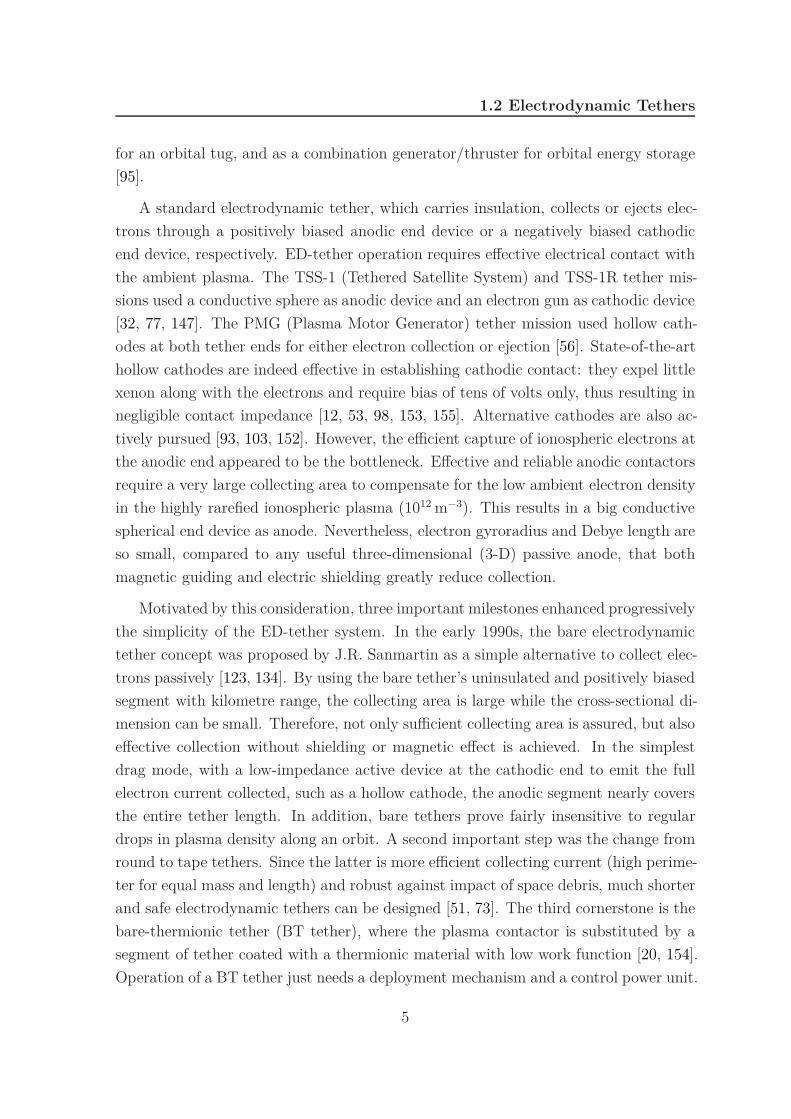
A standard electrodynamic tether, which carries insulation, collects or ejects elec-
trons through a positively biased anodic end device or a negatively biased cathodic
end device, respectively. ED-tether operation requires effective electrical contact with
the ambient plasma. The TSS-1 (Tethered Satellite System) and TSS-1R tether mis-
sions used a conductive sphere as anodic device and an electron gun as cathodic device
[32, 77, 147]. The PMG (Plasma Motor Generator) tether mission used hollow cath-
odes at both tether ends for either electron collection or ejection [56]. State-of-the-art
hollow cathodes are indeed effective in establishing cathodic contact: they expel little
xenon along with the electrons and require bias of tens of volts only, thus resulting in
negligible contact impedance [12, 53, 98, 153, 155]. Alternative cathodes are also ac-
tively pursued [93, 103, 152]. However, the efficient capture of ionospheric electrons at
the anodic end appeared to be the bottleneck. Effective and reliable anodic contactors
require a very large collecting area to compensate for the low ambient electron density
in the highly rarefied ionospheric plasma (1012 m−3). This results in a big conductive
spherical end device as anode. Nevertheless, electron gyroradius and Debye length are
so small, compared to any useful three-dimensional (3-D) passive anode, that both
magnetic guiding and electric shielding greatly reduce collection.
Motivated by this consideration, three important milestones enhanced progressively
the simplicity of the ED-tether system. In the early 1990s, the bare electrodynamic
tether concept was proposed by J.R. Sanmartin as a simple alternative to collect elec-
trons passively [123, 134]. By using the bare tether’s uninsulated and positively biased
segment with kilometre range, the collecting area is large while the cross-sectional di-
mension can be small. Therefore, not only sufficient collecting area is assured, but also
effective collection without shielding or magnetic effect is achieved. In the simplest
drag mode, with a low-impedance active device at the cathodic end to emit the full
electron current collected, such as a hollow cathode, the anodic segment nearly covers
the entire tether length. In addition, bare tethers prove fairly insensitive to regular
drops in plasma density along an orbit. A second important step was the change from
round to tape tethers. Since the latter is more efficient collecting current (high perime-
ter for equal mass and length) and robust against impact of space debris, much shorter
and safe electrodynamic tethers can be designed [51, 73]. The third cornerstone is the
bare-thermionic tether (BT tether), where the plasma contactor is substituted by a
segment of tether coated with a thermionic material with low work function [20, 154].
Operation of a BT tether just needs a deployment mechanism and a control power unit.
5

INTRODUCTION
This disruptive technology is the first fully propellant-less system providing in-orbit
drag and/or thrust. This achievement still needs progress on thermionic materials and
tether-plasma interaction modeling, as discussed in this dissertation.
The fundamental area of electrodynamic tether applications is propellantless trans-
portation [15]. ED-tethers can in principle replace traditional propulsion system on-
board spacecraft, changing the orbit of a satellite without the need for any propellant,
and without limitation on how many times changes can be allowed. The tether can
work at three different modes [131],
• Generator Mode The kinetic energy of the tether-plasma system is converted
into electric energy, as a current inside the tether. The resultant Lorentz force
can be a drag or a thrust depending on the relative velocity between the tether
and the plasma. The most obvious application of an ET tether is as an end-of-
life system to deorbit dead satellites and spent rocket stages in LEO (low Earth
orbit), by using the Lorentz force as a drag.
• Power Generation Mode The current induced can also be used as on-orbit
power generation. It is discovered that, in absence of solar power in LEO, a
combination of ED-tether/rocket, with the tether providing electric power and
the chemical rocket providing thrust is more mass-deficient than a fuel cell [95].
• Motor Mode Using an electrical power supply can reverse the direction of
the current, thus the tether works at motor mode. Considering the propellant
used for reboosting the International Space Station over its lifetime, a study has
shown that a bare ED-tether system of moderate length could save about 80%
of the chemical propellant [45].
Electrodynamic tethers can also be used in some other space and science applications
as [126, 131, 132]:
• Electrically conducting tethers can be used as electrostatic tethers for radiation
belt remediation [63, 94, 158]. Earth’s magnetic field traps a layer of energetic
charged particles, mostly from solar wind and cosmic rays, in the so-called Van
Allen radiation belts. Satellites passing through or orbiting within the belts
require expensive shielding. An electrostatic tether passing these regions can
scatter the energetic radiation particles through the induced potential difference
between the tether and the ambient plasma, deflect these particles such that
6
1.3 Background on Plasma, Sheath and Probe Theory
their post-deflection velocities would fall into the loss cone, and eventually send
some of them out of the radiation belts.
• Current-carrying tethers in low Earth orbit provide unique active experiments
in ionospheric wave excitation. A tether carrying a steady current in the orbital
frame, radiates waves, allowing slow extraordinary (SE), fast magnetosonic (FM)
and Alfven (A) wave emission into the ionospheric cold plasma [44, 133]. Current
modulation in tethers could generate nonlinear, low frequency wave structures
attached to the spacecraft [60]. Whistlers waves could be excited by a planar
array of electrodynamic tethers [121].
• A bare tether over 10 km long in Low Earth Orbit, would be an effective electron-
beam source to produce artificial auroras [96, 127]. Because current will vanish at
both ends and the ion-to-electron mass ratio is large, the tether would be biased
highly negative and attract ions over most of its length. Ions impacting with
keV energies would liberate secondary electrons, which would locally accelerate
away from the tether, then race down geomagnetic lines, excite neutrals in the
ionospheric E-layer, and result in auroral emissions. Tomographic analysis of
auroral emissions from the footprint of the beam, can provide density profiles of
dominant neutral species in the E layer .
• The bare-tether array can be used as the electric solar wind sail, using the dy-
namic pressure of the solar wind for propulsion. The electrostatic field created
by the tethers deflects trajectories of solar wind protons. The flow-aligned mo-
mentum lost by the protons is transferred to the charged tether by a Coulomb
force and then transmitted to the spacecraft as thrust. Because the sheath of
each tether will be much larger than its radius, the virtual electric sail that forms
around each charged tether is typically tens or hundreds of meters in radius, be-
ing millions of times larger than the physical width of the tether wires some tens
of micrometers. As a result the electric sail can be more efficient than a solar
photon sail [69, 70, 71].
1.3 Background on Plasma, Sheath and Probe The-
ory
The genesis of Plasma Physics comes from the Nobel prize winning American chemist
Irving Langmuir, whose achievements ranged from the chemistry of surfaces to cloud
7

INTRODUCTION
seeding for promoting rain. Langmuir worked for the General Electric Co., investigat-
ing the physics and chemistry of tungsten-filament light-bulbs, with a view of finding
a way to greatly extend the life time of the filament. In this process, he developed the
theory of plasma sheaths.
In 1923, from the study of a negatively charged auxiliary electrode immersed in
the path of a mercury arc, he introduced the term ‘sheath’ and wrote in his work
that [82], “ Electrons are repelled from the negative electrode while positive ions are
drawn towards it. Around each negative electrode there is thus a ‘sheath’ of definite
thickness containing only positive ions and neutral atoms. ... The electrode is in fact
perfectly screened from the discharge by the positive ion sheath... ” As his research
progressed, Langmuir later realized that sheaths do contain some electrons near the
sheath boundary.
Fig. 1.1 Positive ion sheaths around grid wires in a thermionic tube containing gas[64].
In 1928, he introduced the word ‘plasma’ as [83], “Except near the electrodes,
where there are sheaths containing very few electrons, the ionized gas contains ions
and electrons in about equal numbers so that the resultant space charge is very small.
We shall use the name plasma to describe this region containing balanced charges of
ions and electrons.” The first figure (Fig. 1.1) with the word plasma appeared in [64],
where it is stated that “Figure 1 shows graphically the condition that exists in such
a tube containing mercury vapor. The space between filament and plate is filled with
a mixture of electrons and positive ions, in nearly equal numbers, to which has been
given the name ‘plasma’ ”. Langmuir conceived the word plasma because the way how
8

1.3 Background on Plasma, Sheath and Probe Theory
an ionized gas, as an electrified fluid, carries electrons and ions reminded him of the
way blood plasma carries red and white corpuscles [100].
After Langmuir, plasma researches gradually spread in a lot of directions, such as
• In Earth’s ionosphere, the atmosphere is ionized and contains a plasma. It
reflects the radio waves, bouncing a transmitted signal down to ground, facilitat-
ing radio communications over long distances. To understand and correct some
of the deficiencies in radio communication, the theory of electromagnetic wave
propagation through non-uniform magnetized plasma are developed [14].
• It has often been said that 99% of the visible matter in the universe is in the
plasma state [58]. The pioneer in astrophysical plasma field was Hannes Alfven,
who developed the magnetohydrodynamics (MHD) theory, which has been suc-
cessfully employed in a wide topics in astrophysics as sunspots, solar flares, solar
wind, star formation, and so on [4].
• Fusion power is the generation of energy by nuclear fusion. In fusion reactions,
two lighter atomic nuclei fuse to form a heavier nucleus, and the lost mass is
converted into energy through E = mc2. The research on fusion power, which
provides the possibility of large scale clean energy production for the future,
is a major part of present plasma physics researches. There are two major
branches of fusion energy research. Magnetic confinement fusion uses magnetic
and electric fields to heat and squeeze the hydrogen plasma, as used in the
International Thermonuclear Experimental Reactor (ITER) project in France
[151]. Inertial confinement fusion uses laser beams or ion beams to squeeze
and heat the hydrogen plasma, an experimental approach being studied at the
National Ignition Facility (NIF) in United States [88].
• Electric thrusters, i.e., plasma thrusters, use electrical energy to accelerate the
ionized propellant to high speeds [68]. This field subdivides into three categories
[67]: electrothermal propulsion, wherein the propellant is electrically heated,
then expanded thermodynamically through a nozzle, e.g., resistojets and arc-
jets; electrostatic propulsion, wherein ionized propellant is accelerated by direct
application of electrostatic forces, e.g., ion thrusters and field emission electric
propulsion; and electromagnetic propulsion, wherein the propellant is accelerated
under the combined action of electric and magnetic fields, e.g., magetoplasma-
dynamic (MPD) thrusters, Hall thrusters, pulsed plasma thrusters, and Helicon
double layer thruster. Electric propulsion provides the possibility of achieving
9

INTRODUCTION
very high exhaust velocities, thus reducing the total propellant burden for space
transportation missions.
• Plasma diagnostics is a field devoted to devising, developing and proving tech-
niques for measuring the properties of plasmas [65, 108]. To deduce information
about the state of the plasma from practical observations of physical processes
and their effect, it requires a profound understanding of the physical processes
involved. Plasma diagnostics contains broad topics as probe diagnostics, optical
methods (e.g., spectroscopy and interferometry), microwave diagnostics, diag-
nostics with particle beams, et cetera.
Langmuir probe is probably the simplest and most widely used form of plasma
diagnostic. It consists of a metallic wire, sphere or disk, which is inserted into a plasma
and electrically biased with respect to the plasma to collect electron and/or positive
ion currents. By measuring the probe voltage-current characteristic, it can deduce
the local properties of a plasma, such as potential, temperature, and density [26, 61].
However, the plasma potential is quite difficult to estimate from the characteristics
of collecting probes. This maybe overcome by use of an emissive probe, which is
typically made of a fine loop of tungsten wire, normally being heated to emit current
[136, 137]. When the probe is biased sufficiently positive with respect to the plasma,
the electrons will be drawn back to the probe and no difference should be observed
between the characteristics of a hot or cold probe. But when the probe is negatively
biased, emitted electrons will flow across the sheath and the hot-probe and cold-probe
characteristics begin to disagree, which is an indication of the space potential [18, 23].
However, both Langmuir probe and emissive probe are not as simple as it may seem.
From experimental point of view, they are intrusive techniques, being not remote,
thus requiring careful design so as not to interfere with the plasma nor be destroyed
by it. From theoretical point of view, the interpretation of the current-voltage curves
is difficult.
To study how the plasma parameters are related to probe characteristic, we need
to study the problem of sheath formation on actual probes. All plasma phenomena
can be described by combing Maxwell’s equations with the Lorentz force equation [54].
They are equations from experimental observation, modeling the physical reality of
10

1.3 Background on Plasma, Sheath and Probe Theory
plasma. Maxwell’s equations are
∇ · E =1
ǫ0ρ Gauss’s law , (1.1a)
∇ · B = 0 Gauss’s law for magnetism , (1.1b)
∇ × E = −∂B
∂tMaxwell-Faraday equation , (1.1c)
∇ × B = µ0J + µ0ǫ0∂E
∂tAmpere’s law with Maxwell’s correction , (1.1d)
which introduce the electric field E, the magnetic field B. The field and the particles
interact over time t through the charge density ρ and the current density J . The
universal constants in the equations are vacuum permittivity ǫ0 ≈ 8.854 × 10⁻¹⁷ F m−1
and vacuum permeability µ0 ≈ 1.257 × 10⁻⁶ N A−2. The Lorentz force law,
F = q (E + v × B) , (1.2)
gives the force F experienced by a particle of charge q moving with velocity v in an
electric field and magnetic field, thus describing how the electric and magnetic field
act on charged particles and currents.
Maxwell’s equations and the Lorentz force law give exact and complete description
of plasma motions. However they are not useful, because it is impractical to follow the
complicated trajectories of all particles in plasma, whose density can easily be more
than 1011 m−3. As a result, a variety of statistical models of plasma dynamics have
been developed.
• Classical microscopic theory, which,for instance, solves the interacting tra-
jectories of a large number of particles using Newton second law, is unimaginable
even considering the most advanced computers today. Neither it is desirable to
do so because the solutions acquired would be mostly irrelevant information
which requires another advanced computers to extract the useful messages.
• Fluid theory only takes into account the motion of fluid elements, neglects
the identity of the individual particle and derives equations directly for plasma
density and current. It is the simplest description of a plasma, being less com-
putationally expensive. Nevertheless, it is valid generally near thermodynamic
equilibrium, being inadequate in some phenomena.
• Kinetic theory, applying statistical probability concepts, derives macroscopic
plasma parameters (e.g, temperatures, densities, currents, et cetera) from the
11

INTRODUCTION
distribution of particle in phase space - a space that combine both the velocity
and the position information. Kinetic models are valid over a broad range of
physical phenomena and are more computationally practical than classical mi-
croscopic models, although being computationally more expensive compared to
fluid models. Examples of kinetic equations are the Boltzmann equation and
Vlasov equation.
1.4 Dissertation Outline
A new material, C12A7 : e− electride, which might present a work function as low
as 0.6 eV and moderately high temperature stability, is recently proposed as coating
for floating bare tethers [154]. Arising from heating under space operation, current
is emitted by thermionic emission along a thus coated cathodic segment. Thermionic
emission, being much more efficient than ion collection at the cathodic segment, may
eliminate the need for an active cathodic device and its corresponding gas feed require-
ments and power subsystem, which results in a truly “propellant-less” tether system
for such basic applications as de-orbiting LEO satellites.
Thermionic emission is different from hollow cathode emission in important aspects
concerning a tethered system:
• Only electrons, rather than plasma, are emitted
• Cylindrical rather than spherical geometry is involved, which allows for collected
ion current to follow OML law
• A relatively definite physical law for emission current is involved, which is not
the case for a hollow cathode, for which broadly different regimes may exist,
giving rise to quite different schemes/analyses
• Thermionic emission allows the current to be emitted over a long segment of
tether under a range of voltage-bias values, other than being emitted only at
tether end using plasma contactors as hollow cathodes
• Use of laboratory test results in designing hollow cathodes for generic use in
space is tricky.
To study the operation of bare thermionic tethers, it is critical to model the plasma-
tether contact along all the tether length, which is the main goal of this thesis. As
the theory on the anodic contact has been well developed, we will focus on solving the
12

1.4 Dissertation Outline
stationary sheath around an electron-emitting probe in the absence of collisions and
magnetic fields, by the use of kinetic theory, which is still not yet well developed in
the theory for emissive probes.
In Chap. II, we will first introduce the basics to understand this thesis, such as
electrodynamic tether principles and orbital-motion-limited theory. What will be de-
scribed in this chapter is crucial for the development of the theory and the calculations
in later chapters.
In Chap. III, a preliminary study on the space-charge-limited (SCL) double sheath
in front of the cathodic segment is presented using Langmuir’s SCL electron current
between cylindrical electrodes and orbital-motion-limited ion-collection sheath. A de-
tailed calculation of current and bias profiles along the entire tether length is carried
out, with ohmic effects and the transition from SCL to full Richardson-Dushman emis-
sion included. Although this first model provides a very simple and fast derivation
of the drag production using BT tethers, it is still a crude model. A thorough study
of the sheath formation around cylindrical eletron-emitting probes is still necessary.
For this reason, two complementary studies will be carried out using analytical and
numerical methods.
In Chap. IV, at the conditions of high bias and relatively low emission that make
the potential monotonic, an asymptotic analysis is carried out, extending the OML
ion-collection analysis to investigate the probe response due to electrons emitted by
the probe. At a given emission, the space charge effect from emitted electrons increases
with decreasing magnitude of negative probe bias. Although emitted electrons present
negligible space charge far away from the probe, their effect can not be neglected in
the global analysis for the sheath structure and two thin layers in between sheath and
the quasineutral region. The space-charge-limited (SCL) condition is located. And a
crude model to carry out the longitudinal analysis is presented for weak ohmic effects.
In Chap. V, we will use orbital motion theory to model all species existing for
an emissive probe, being plasma electrons, plasma ions and emitted electrons. And
potential is no longer considered monotonic, with a potential hollow allowed. Also the
probe radius can be arbitrary. The Poisson-Vlasov system is described by an integro-
differential equation, which is discretized using finite difference method. The non-
linear algebraic equations are solved using a parallel implementation of the Newton-
Raphson method. And results are compared with those using analytical methods.
13


Chapter 2
BASICS ON THE STUDY
2.1 Electrodynamic Tether Basics
2.1.1 Induced Current and Lorentz Force
It is well known that the electromagnetic field shows relativistic effects. For instance,
an observer measuring a charge at rest would detect a static electric field without
magnetic, while a magnetic field around a current would be detected by another ob-
server moving toward or away from the charge. The theory of special relativity gives
how electrodynamic objects, especially electric and magnetic fields, are altered under
a Lorentz transformation from one inertial frame to another. For a general Lorentz
transformation from K to a system K ′ that moves with velocity v relative to K, the
transformations between electric field E and magnetic field B are [66]
E′ = γ (E + v × B) + (1 − γ)E · v
v2v , (2.1)
B′ = γ(
B − 1
c2v × E
)+ (1 − γ)
B · v
v2v , (2.2)
where c is the speed of light and γ = 1/√
1 − v2/c2 is the Lorentz factor. In non-
relativistic transformation, i.e., for v ≪ c, the Lorentz factor has γ ≈ 1, which conse-
quently yields the transformations
E′ ≈ E + v × B , (2.3)
B′ ≈ B − 1
c2v × E ≈ B . (2.4)
15

BASICS ON THE STUDY
A non-relativistic transformation relates the electric fields, in the frames moving
with tether and local ambient plasma [132],
ET etherF rame − EP lasmaF rame = (vt − vpl) × B , (2.5)
where the planetary magnetic field B is common in both frames, and vt and vpl are
the velocities of tether and plasma relative to the planet. In the highly conductive
plasma away from the tether, the electric field is negligible in the frame moving with
the plasma. Then, the electric field Em introduced by motional electromotive force,
the same as the electric field outside the tether yet in the tether frame, can be written
as
Em = EOutside = ET etherF rame = (vt − vpl) × B . (2.6)
For a passive tethered system operating at generator mode, this motional field Em
drives a current I with
I · Em > 0 . (2.7)
An insulated tether with length L, carrying a uniform current, would in turn experience
a Lorentz force
F = LI × B . (2.8)
The resultant Lorentz force transfers a net mechanical power to the tether-plasma
interaction,
Wm = LI × B · (vt − vpl) = −LI · Em < 0 . (2.9)
The lost power appears as the current in the tether electric circuit. Since the power
transferred to the tether is
Wt = LI × B · vt , (2.10)
the Lorentz force acts as a drag (Wt < 0) on the tether if vt is in the same direction
as vt − vpl, otherwise a thrust (Wt > 0).
For a vertical tether flying in an equatorial orbit in LEO and a non-tilted centered
magnetic dipole model, Fig. 2.1 shows the direction of relative velocity and Lorentz
force in the prograde case. If the plasma is considered as corotating with the planet,
then, for circular equatorial orbits with radius smaller than the geostationary orbit ,
Lorentz force acts as a drag for both retrograde and prograde orbit (Fig. 2.1). However,
outside the geostationary orbit, Lorentz force acts as a thrust for prograde orbits as
shown in (Fig. 2.1), or as a drag for retrograde orbits. For a Jupiter mission, because
of both a rapid spin and low mean density, the stationary orbit in Jupiter is around
16

2.1 Electrodynamic Tether Basics
2.24 times the Jovian radius. Together with the strong magnetic field, the Lorentz
force on a tether in prograde Jovian orbit beyond the stationary orbit would be a
thrust [130].
e−
Em
N
Inside stationay orbit
Magnetic field pointing North
e−
Em
Thrust e−
e−
e−
e−
Outside stationay orbitΩtether < Ωplanet
Ωtether > Ωplanet
Ωplanet
Rs
vrel
Ωtether
vrel Drag
Ωtether
Fig. 2.1 Drag or thrust for electrodynamic tethers subjected to motional electromotiveforce. The ED-tether system rotates around the planet at different prograde circularequatorial orbits. The plasma is considered corotating with the planet. Rs is thegeostationary-orbit radius.
In general, for non-zero orbital inclination and a realistic magnetic model, the
component of B, that is perpendicular to the orbital plane, drives the current along
the tether through Em, i.e., the projection of Em along the tether, and produces
useful Lorentz force. For spacecraft in LEO, this Lorentz force acts a drag, being an
ideal passive method for deorbiting end-of-life spacecraft. The components of B that
are inside the orbital plane result in negligible potential difference across the tether.
However, the resultant perpendicular Lorentz force pushes tether off the orbital plane
and may lead to a coupled in-plane/off-plane unstable periodic motion [107].
Using geomagnetic dipole model with the magnetic axis of the dipole tilted off
from the spin axis by approximately 11.5°, the perpendicular component of magnetic
field is given by [49]
B = BE
(RE
r
)3
cos i , (2.11)
where i is the orbital inclination, RE ≈ 6378 km is the Earth radius, and BE ≈ 3100 T
is the magnetic field at magnetic equator of the Earth. The typical altitude range of
17

BASICS ON THE STUDY
LEO satellites goes from 750 to 1500 km. For a 1000 km height, the orbital velocity is
around 7350 m s−1, being much faster than the corotating plasma with 536 m s−1. In
this thesis, we will often consider a typical motional field for orbits with height around
1000 km as
Em = (vt − vpl) × B ≈ 7.5 km s−1 × 2000 T = 150 V km−1 . (2.12)
2.1.2 Current Closure Loop for An Insulated Tether
For a tether in drag mode, electrons inside the tether would move towards the higher
potential resulted from motional electromotive force, as driven by the motional field
along the tether Em. Consequently, a current tends to flow in the same direction as Em.
For a current to flow inside the tether, the circuit must be closed by current exchange
through the interaction with the surrounding plasma. This interaction arises from the
difference between the potential inside the tether, Vt, and the plasma potential, Vpl.
Em · L
∆VA
B
C
A
e−
e−
I
V
Vpl Vt
without ohmic effects
∆VL
Vpl Vt
∆V
V
Em
∆VA
Em · L
with ohmic effects
yy−∆VC −∆VC
Fig. 2.2 Schematic of tether potential Vt and plasma potential Vpl in the tether framefor a standard ED tether at drag mode.
The potential in the plasma, outside the tether, however in the tether frame, arises
from the motional electromotive force:
Vpl (y) = Vpl
∣∣∣y=0
+ Emy , (2.13)
18

2.1 Electrodynamic Tether Basics
where y is the spatial coordinate along the tether which is defined positive following
the moving direction of the electrons, as shown in Fig. 2.2 for an insulated tether in
drag mode. The plasma potential depends on the ambient conditions and the motion
of the tether, instead of tether characteristics. Here we assume that Em does not
change along the tether.
The tether potential Vt follows Ohm’s law,
Vt(y) = Vt
∣∣∣y=0
+y
σcAt
I , (2.14)
where σc is the tether conductivity and At is the cross-sectional area of the tether.
If we neglect ohmic effects, as σc → ∞, the tether is equipotential. If ohmic effects
are not negligible, the tether potential depends on the tether characteristics and the
current. Since the current I is constant along the tether due to insulation, Vt decreases
linearly from A to C as in Fig. 2.2.
For an insulated tether, electrons are collected from the ambient plasma by a
plasma contactor at the anodic end of the tether, where the tether is positively biased
to the plasma, i.e., the tether-to-plasma potential being ∆VA = Vt
∣∣∣y=0
− Vpl
∣∣∣y=0
> 0.
The collected current is emitted by another plasma contactor at the cathodic end with
∆VC = Vt
∣∣∣y=L
−Vpl
∣∣∣y=L
< 0. Thus, current exchange with plasma through end devices
accomplishes the circuit of the current that is driven by Em and flows from C to A .
Subtracting Eq. (2.13) from Eq. (2.14) gives the circuit equation of this system,
EmL = ∆VA +L
σcAtI − ∆VC . (2.15)
This equation indicates that the tether, self-consistently and passively, adjusts its
potential Vt and establishes a current I that is able to be collected by ∆VA > 0,
emitted by ∆VC < 0, and allowed by the motional electromotive force EmL and its
own conductance σcAt/L.
Because plasma contactors requires potential difference relative to the plasma to
exchange current, we have ∆VA > 0 and ∆VC < 0. If in an ideal situation where perfect
plasma contactors are made with no load impedance, |∆VA| = 0 and |∆VC | = 0, the
resultant induced current becomes the short circuit current, given by Eq.(2.15) as
I∗ = σcAtEm , (2.16)
being the maximum current allowed for a tether in drag mode.
19

BASICS ON THE STUDY
e−
A
C
y y
I
e− Vps Vps
∆VA
L
without ohmic effects with ohmic effects
∆V∆V
∆VA
Em
powersupply
VtVt
VV
it is presented here just to show the total potential drop.
−∆VC
Vpl Vpl
−∆VC Em · L Em · L
this is not the real potential line inside the power supply
Fig. 2.3 Schematic of tether potential Vt and plasma potential Vpl in the tether framefor a standard ED tether at motor mode.
When the motional electromotive force can only produce drag, an external power
supply Vps is required to overcome the motional field, to reverse the direction of the
current and thus to produce thrust. Now the tether is said to operate at the motor
mode, transforming the electrical energy to kinetic energy. Although this will not be
discussed in the rest of this work, it will be presented here for completeness. As shown
in Figure 2.3, the circuit equation of this system is
Vps = ∆VA +L
σcAtI − ∆VC + EmL . (2.17)
As in the previous case, ohmic effects are considered and other possible loads are
neglected. The current and the tether potential are established self-consistently by the
tether following the constraints given by the ability of anodic collection and cathodic
emission, the motional electromotive force, its own conductance, and the electric power
supply.
In the previous models for both drag and motor modes, not all impedances are
considered. The impedances in a tether-plasma system can conveniently be grouped
into four categories [60]. First, there is the intrinsic resistance of the tether itself,
L/σcAt. Second, arising from the electrical contact between plasma contactors and
20

2.2 Theories of Sheath around a Probe
ionosphere, the potential drop at tether ends, ∆VA or ∆VC , being (normally nonlinear)
functions of I, can be considered as related to I though an impedance. Third, there are
impedances associated with the electrical subsystems for the tether, RL. Fourth, there
are radiation impedances due to the excitation of electromagnetic waves in plasma, Zr.
We have only considered the first two kinds of loads. Including all loads, Eqs. (2.15)
and (2.17) become
EmL = ∆VA +L
σcAtI − ∆VC + IZr + IRL , (2.18)
Vps = ∆VA +L
σcAtI − ∆VC + EmL + IZr , (2.19)
where the load resistance has been included in the Vps for the motor mode. It can
also be said that the self-consistent current in the tether is determined by all the
impedances in the tether-plasma system. References [38, 117] have given studies on
tether system in a more realistic environment, considering all impedances and using
nonlinear models for plasma contactors. For simplification, we will keep on assuming
both radiation impedance and load resistance negligible compared to the other two
kinds of impedances.
The performance of an insulated tether is limited by the inefficient anodic current
collection. Thus the bare-tether concept was proposed to to be more effective than
large conductive spheres at the tether anodic ends. The small cross-sectional dimension
of the tether allows it to collect electrons over the resulting positively biased (anodic)
segment as a giant cylindrical Langmuir probe. The full electron current is emitted
through a low-impedance cathodic device, such as a hollow cathode, located at the
cathodic end of the tether. In the absence of a low-impedance device, bare thermionic
tethers not only collect but also emit currents by the tether itself. With a low-work
function material as a coating on the cathodic segment of the tether, the current
exchange can be efficient and thus produce useful drag force. This technology is the
first fully propellant-less system providing in-orbit drag. To study the operation of
bare thermionic tethers, we have to first understand the plasma-probe interactions.
2.2 Theories of Sheath around a Probe
2.2.1 Distribution Function in Phase Space
To completely specify the dynamical state of a particle, we use the phase space of a
system, which contains both position space, r = (x, y, z), and velocity space (v =
21

BASICS ON THE STUDY
vx, vy, vz). Now, we can define the velocity distribution of the particles, f(r, v, t),
which gives the number of particles per m3 at position r and time t with velocity
components between vx and vx + dvx, vy and vy + dvy, and vz and vz + dvz,
f (x, y, z, vx, vy, vz, t) dvx dvy dvz ≡ f (r, v, t) d3v , (2.20)
where d3v stands for a three-dimensional volume in velocity space, i.e., dvx dvy dvz . If
f(r, v, t) is independent of r, the distribution is homogeneous. If f(r, v, t) is indepen-
dent of the direction of v, the distribution is isotropic. The particle number density,
as a function of four scalar variables (x, y, z, t), can be found from the integral of the
velocity distribution function as
N(r, t) =∫
∞
−∞
f (r, v, t) d3v . (2.21)
The current density for a given species with charge q thus becomes
j (r, t) = q∫
∞
−∞
vf (r, v, t) d3v . (2.22)
The average particle kinetic energy becomes
Eav (r, t) =1
N(r, t)
∫∞
−∞
mv2
2f (r, v, t) d3v , (2.23)
where m is the mass of the particle. In plasma physics, the average kinetic energy Eav
is closely related to the temperature T , a constant that characterizes the width of the
distribution.
The most probable distribution for a gas in thermal equilibrium is the Maxwellian
distribution function [19],
fM (vx) = N(
m
2πKT
)1/2
exp
(− mv2
x
2KT
), in one dimension,
(2.24)
fM (vx, vy) = Nm
2πKTexp
(−
mv2x + mv2
y
2KT
), in two dimensions,
(2.25)
fM (vx, vy, vz) = N(
m
2πKT
)3/2
exp
(−mv2
x + mv2y + mv2
z
2KT
), in three dimensions,
(2.26)
22

2.2 Theories of Sheath around a Probe
being both homogeneous and isotropic. The constant K ≈ 1.38 × 10⁻²³ K−1 is the
Boltzmann’s constant. The average kinetic energy becomes
Eav =(
m
2πKT
)3/2
×∫
∞
−∞
∫∞
−∞
∫∞
−∞
mv2x + mv2
y + mv2z
2exp
(−mv2
x + mv2y + mv2
z
2KT
)dvx dvy dvz
=(
m
2πKT
)3/2 ∫ ∞
0
mv2
2exp
(− mv2
2KT
)4πv2 dv
=3
2KT , in three dimensions, (2.27)
with Eav = KT/2 in each dimension. It is customary to give temperatures in units of
energy. To avoid confusion on the number of dimensions involved, it is not T but the
energy corresponding to KT that is used to denote the temperature, using electronvolt
eV as the units. For KT = 1 eV ≈ 1.6 × 10⁻¹⁹ J, the corresponding temperature in
kelvin is
1 eV =e
K=
1.6 × 10⁻¹⁹
1.38 × 10⁻²³≈ 11 605 K . (2.28)
By a plasma with temperature 2 eV, we mean that it has average energy Eav = 3 eV
in three dimensions, with Eav = 1 eV in each dimension. Note that the ions and
the electrons in a plasma often have separate Maxwellian distributions with different
temperatures Ti and Te. Each species can be in its own thermal equilibrium.
2.2.2 Poisson-Vlasov System with Stationary Electric field
and without Magnetic Field
In an electrostatic plasma, without magnetic field, Maxwell equations, Eqs. (1.1), are
reduced to Gauss’s law for electricity and Faraday’s law of induction as
∇ · E =ρ
ǫ0, ∇ × E = 0 . (2.29)
Since the curl, ∇×, of the electric field is zero, a scalar electric potential Φ is defined
as
E = −∇Φ. (2.30)
23

BASICS ON THE STUDY
It is the work done on a unit charge in reaching the point from an arbitrary reference
point (usually infinity). Thus we can derive Poisson’s equation as
∇2Φ = −∇ · (−∇Φ) = −∇ · E = − ρ
ǫ0, (2.31)
which is one of the two equations to relate the potential and space charge at a local
position in plasma.
The other equation to relate the potential and the space charge is Lorentz’s law. In
kinetic theory, it is not necessary to describe each particle’s trajectory using Lorentz’s
law. Instead, it describes the evolution of a charge density distribution function in
phase space, f(r, v, t), as described in Sec. 2.2.1. In a thermodynamic system not in
thermodynamic equilibrium, the Boltzmann equation describes the statistical behavior
of the system as
df
dt=
∂f
∂t+
(∂f
∂t
)
diff
+
(∂f
∂t
)
force
=∂f
∂t+ v · ∂f
∂r+
F
m· ∂f
∂v
=∂f
∂t+
∂f
∂x
dx
dt+
∂f
∂y
dy
dt+
∂f
∂z
dz
dt+
∂f
∂vx
dvx
dt+
∂f
∂vy
dvx
dt+
∂f
∂vz
dvz
dt
=
(∂f
∂t
)
coll
. (2.32)
The terms (∂f/∂t)force , (∂f/∂t)diff , and (∂f/∂t)coll account for the force exerted on
the particles, the diffusion of particles, and the collision among particles, respectively.
The term ∂f/∂t is the explicit dependence of f on time for fixed values of v and r.
The convective derivative, df/ dt, can be interpreted as the rate of change as seen in
a frame moving with the particles in six-dimensional phase space (r, v).
In a sufficiently hot plasma, where collisions can be neglected and the force F is
given by the Lorentz’s law, the Boltzmann Equation becomes
df
dt=
∂f
∂t+ v · ∂f
∂r+
q
m(E + v × B) · ∂f
∂v= 0 , (2.33)
which is called the Vlasov equation. Vlasov equation conserves the distribution func-
tion along the particle orbits as df/ dt = 0. If a group of particles in an infinitesimal
volume element dr dv have a density f(r, v, t = 0) in this phase space (r, v), af-
ter some time t′, they arrive at another phase place (r′v′) with the density being
f(r′, v′, t′) = f(r, v, t = 0).
24
2.2 Theories of Sheath around a Probe
In a stationary plasma, the distribution function becomes time independent. The
procedure for calculating the space charge can thus be simplified by considering the
orbital motions of particles without concern on time. Again, we consider a group of
particles in an infinitesimal volume element dr dv. This group of particles have a
velocity v0 at the position where they originate from, say r0. They move in the space
following Lorentz’s law, describing an identical orbit. At any position that this orbit
can arrive, this group of particles contribute to the space charge there, with their
density being f(r, v) = f(r0, v0). Since the plasma is time-invariant, particles with
this initial velocity, being continuously supplied from their origin, always contribute
to the total space charge where their orbit passes. Therefore, at any position in space
r, the number density is an integral of the distribution function of all the particles
whose orbits can cross r,
N (r) =∫ vb
va
f (r, v) dv =∫ vb0
va0
f (r0, v0) dv , (2.34)
over proper velocity ranges that characterize these orbits, being [va, vb] at r and
[va0, vb0] at their origin r0.
For electrostatics plasma, the Lorentz force takes the form as
F = qE . (2.35)
Electric force is a conservative force, with the property that the work done in moving
a particle between two points is independent of the taken path. This again simplifies
the description of orbital motions. In the next section will present the orbital motion
theory in a collisionless, unmagnetized, and stationary plasma, with cylindrical geom-
etry. In later chapters, we will use this simplified Poisson-Vlasov model to solve the
sheath formation around an emissive probe.
2.2.3 Orbital-Motion-Limited Theory
Orbital motion has been first presented by Mott-Smith and Langmuir in 1926 [101]. If
the gas pressure is so low that collisions in the sheath are negligible. For a collecting
probe, without any particle emission from the probe, the charged particles from the
ambient plasma describe free orbits, some of which end on the surface of the collector.
If the equipotentials are coaxial cylinders, the condition for a particle to reach the
collector depends only upon the initial and final potentials and the initial velocities
of this particle, not upon the nature of the field of force along the whole orbit. The
25

BASICS ON THE STUDY
total current to the collector can thus be found by summing the contributions of all
species, which is a purely mechanical problem. The current, being a function of the
potential drop in the sheath and of the sheath radius only, requires another relation
among these three variables. This is found by solving a space charge problem, which
calculates the potential distribution in the sheath using Poisson’s equation.
Orbital-motion-limited (OML) theory has been well studied by J.R. Sanmartin
using asymptotic methods [43, 128], and comparisons with numeric results from both
steady-state Vlasov calculations [124] and particle-in-cell simulations [46] have shown
excellent agreements. Here we make a simple description of OML electron collection
by a probe positively biased at a potential Φp > 0 with respect to the plasma, only
to understand the concept of OML current. It also serves an example for the orbital
motion limited collection for any species of particles that is attracted by a probe either
negatively or positively biased. The next chapter will quantitatively elaborate this
theory for studying thermionic emission. We also consider high bias (|eΦp| ≫ kTe ≈0.1 eV), a collisionless, stationary, and unmagnetized plasma and two dimensional
cylindrical geometry, as in the literature and in the rest of this thesis.
Integration over energy and momentum space
For a positively biased probe without emission, all electrons originate at infinity, r →∞. In a central force field where cylindrical symmetry prevails, two initial velocities,
being the radial velocity vr0 and the azimuthal velocity vθ0, characterize the orbit.
Equivalent to vθ0 and vr0, two constants of motion suffice to characterize the orbit,
being transverse energy E and angular momentum J ,
E =mv2
r
2+
mv2θ
2− eΦ(r) , J = mrvθ , (2.36)
where r is the radial distance from the probe center, Φ(r) is the potential with respect
to infinity, thus E being positive but J covering both positive and negative values.
Electrons originate from the ambient plasma at infinity, with a homogeneous
Maxwellian distribution there. From Eq. (2.25), we can rewrite the distribution func-
tion as
fM (E, J) = N∞
m
2πKTeexp
(− E
KTe
), (2.37)
where N∞ = Ni∞ = Ne∞ is the plasma density of the quasineutral plasma at infinity.
Since the Vlasov equation conserves the distribution function along the orbit, the
26

2.2 Theories of Sheath around a Probe
electrons with the energy E and angular momentum J would have a density at r as
f(r, E, J) = N∞
m
2πKTeexp
(− E
KTe
), if the orbit can arrive at r, (2.38)
f(r, E, J) = 0 , if the orbit can not arrive at r. (2.39)
To obtain the electron number density at r, the integration over velocity range can be
transformed to an integration over EJ-space. The rule for change of variables says
dE dJ =
∣∣∣∣∣∂(E, J)
∂(vr, vθ)
∣∣∣∣∣ dvr dvθ , (2.40)
where Eqs. (2.36) yield the Jacobian,
∂(E, J)
∂(vr, vθ)=
∣∣∣∣∣∣mvr mvθ
0 mr
∣∣∣∣∣∣= −m2rvr . (2.41)
The change of variables (vr, vθ) → (E, J) implies
dvr dvθ =dE dJ
m2rvr=
dE dJ
m√
J2r (E) − J2
, (2.42)
with J2r (E) defined as
J2r (E) ≡ 2mr2 [E + eΦ(r)] , (2.43)
being a function of both r and E. The particle density at r can thus be found by the
integrationN(r)
N∞
=∫ Eb
Ea
∫ Jbr(E)
Jar (E)
exp(−E/KTe) dE dJ
πKTe
√Jr
2(E) − J2, (2.44)
over proper EJ-domain that comprises the values characterizing all the orbits arriving
at r. The E-integral covers only positive values by definition. By writing dJ → 2 dJ ,
the J-integral is made to cover just positive values, Ja,br (E) > 0. In the whole thesis,
we always use Jr(E) > 0. Now we should study the orbital motion to identify the
orbits that can arrive at r.
Cutoff and absorption boundaries of orbital motions
For an electron coming from infinity, as long as the equation
J2 − J2r (E) = −m2
er2v2r < 0 , (2.45)
27

BASICS ON THE STUDY
is satisfied, it continues moving inwards. If there is J2 = J2r (E) at some r, because of
the resultant vr = 0, the angular velocity of the particles causes the electrons to move
back towards the infinity. We say that there is a barrier for this electron at this radius
r that would repel the electron back.
r
b
c
a
R
Increasing
Angular
Momentum
d
R
Absorption
Boundary
Increasing
Angular
Momentum
Fig. 2.4 Family of electron orbits corresponding to the same total energy E and variousvalues of angular momentum J . R is the probe radius. Left: (a) and (b), no potentialbarrier at any radius; (c), no barrier outside r, but with a barrier between r and theprobe; (d), with a barrier outside r. Right: An absorption boundary outside R.
For an observer at r, depending on the potential Φ(r) and the EJ-values of the
electrons, the electrons may describe three kinds of orbits:
• If a potential barrier exists outside r, the electron is reflected back to infinity
before arriving at r (d in Fig. 2.4).
• If a potential barrier exists inside r, the electron would first pass r, continuing
moving inwards, and then return at some radius between r and the probe radius
R. Again, it passes r, but moving outwards towards infinity (c in Fig. 2.4).
• If there is no any potential barrier at all for any radius outside R, the particle
would strike on the probe and be collected by the probe (a and b in Fig. 2.4).
For a sequence of orbits corresponding to some given energy E but various angular
momentum J , at any radius r, Eq. (2.45) sets a cutoff boundary [76],
J2 ≤ J2r (E) ≡ 2mer
2 [E + eΦ(r)] , (2.46)
28

2.2 Theories of Sheath around a Probe
beyond which the particles can not exist at r, i.e., it is impossible for the orbits to
cross r. For any energy E ≥ 0, it is always possible to find some values of J to satisfy
the cutoff boundary. The constraint on E is thus trivial. The reason is that electrons,
attracted by the positively biased probe, move towards the probe with increasing ki-
netic energy and decreasing potential energy. There is no requirement for the electrons
to have enough energy so that it can overcome the electric potential barrier. Instead,
the angular momentum needs to be small enough, so that the azimuthal velocity vθ is
small enough to have v2r 6= 0.
For ions coming from plasma at infinity, because their kinetic energies decrease
while moving inwards, there are constraints for both energy and angular momentum.
Most of the ions, except the few with high energy at the tail of the distribution function,
are reflected or repelled back to infinity by the positively biased probe. The plus sign
in Eq. (2.46) is changed to a minus sign and the cutoff boundary becomes
J2 ≤ J2r (E) ≡ 2mir
2 [E − eΦ(r)] , for plasma ions. (2.47)
Because J2r (E) of ions decreases with decreasing r, if Eq. (2.47) is satisfied at r, it
is satisfied at any radius with r′ > r. As a result, satisfying the cutoff boundary is
sufficient to permit ion orbits to arrive at r. Equation (2.47) sets constraints on both
energy and angular momentum,
E ≥ eΦ(r) and J ≤ Jr(E) for ion orbits to arrive at r. (2.48)
Part of these ions will arrive at the probe and absorbed by the probe, because of
E ≥ eΦp and J ≤ JR(E) for ion orbits to arrive and disappear at R. (2.49)
Rest of the ions, that are repelled back to infinity at somewhere between R and r,
would appear at r again however moving outwards.
Nevertheless, things are not that easy in the case of electrons, although there is no
constraint on energy E. For electrons, Jr(E) in Eq. (2.46) does not always decrease
with decreasing r. In a possible situation, for a radius r and electrons with a given
energy E, if there is Jr > Jr′(E) for some r′ > r, a particle with Jr′(E) < J ≤ Jr(E)
can not arrive at r even though the cutoff boundary in Eq. (2.46) is satisfied. As a
result, for an electron with energy E to arrive at r from infinity, its angular momentum
must satisfy the cutoff boundary at r and everywhere beyond r, which is called the
29

BASICS ON THE STUDY
absorption boundary,
J2 ≤ J∗2r (E) ≡ minJ2
r′(E) : r′ ≥ r . (2.50)
In the literature for orbital-motion-limited theory [43, 128], this absorption boundary
J∗2r (E) is also named as a barrier which reduces the number of electrons to arrive
at r although allowed by the conditions at r. If we say that there is no barrier for a
radius r, it means J∗
r (E) = Jr(E). This meaning of the word barrier will be used in
the rest of the thesis.
J2 = J
2
r(E)
J2 = J
∗2
r(E)
J2 = J
∗2
R(E)
J2
E
Fig. 2.5 Schematic of cutoff boundaries and absorption boundaries in EJ-plane. Thesolid line J2 = J2
r (E) is the cutoff boundary for r. The solid curve J2 = J∗2r (E) is the
absorption boundary for r. The solid curve J2 = J∗2R (E) is the absorption boundary
for probe radius R.
Let us visualize the boundaries on the EJ-plane, or on the (E, J2) plane if strictly
speaking. According to Eq. (2.46), J2 = J2r (E) defines a straight line as shown in
Fig. 2.5, named as r-line since it is characterized by r. It has a slope of 1/2mer2,
increasing with r decreasing. The J2-intercept is 2mer2eΦ(r). Below this line, particles
are forbidden to exist. According to Eq. (2.50), the absorption boundary for r, J2 =
J∗2r (E), determined by the family of r′-lines for all r′ ≥ r , lies at the left of r-line.
This curve J2 = J∗2r (E) can, or part of it can, coincide with the r-line, but never on
the right of it as Jr ≥ J∗
r by definition. Below this curve, particles cannot arrive at
r. For the particles whose EJ-values lie on the left of J2 = J∗2r (E), they can arrive
at r as incoming population (vr < 0). Part of them will be absorbed by the probe if
their EJ-values lie on the left of the absorption boundary for R, J2 = J∗2R (E). The
rest of them will be repelled back at some radius between r and R, crossing r again
as outgoing population (vr > 0).
30

2.2 Theories of Sheath around a Probe
In this section, we will not go into the detail of J∗
r (E), which will be covered in the
section for emissive probe sheath formation study. At this moment we will only give
the densities using J∗
r (E), and define the orbital-motion-limited current.
Ion density and electron density
Given by Eqs. (2.48) and (2.49), with J2r (E) defined in Eq. (2.47) for ions, the ion
density at r is composed of two populations, one being incoming population,
Di = (E, J) : E ≥ eΦ(r) ; J ≤ J∗
r (E) = Jr(E) , (2.51)
the other one being outgoing population,
Do = Di \ Dp , Dp = (E, J) : E ≥ eΦp ; J ≤ J∗
R(E) = JR(E) . (2.52)
Following Eq. (2.44), the ion density at r becomes
Ni(r)
N∞
=∫
∞
eΦ(r)
∫ Jr(E)
0
2 exp(−E/KTi) dE dJ
πKTi
√Jr
2(E) − J2
−∫
∞
eΦp
∫ JR(E)
0
exp(−E/KTi) dE dJ
πKTi
√Jr
2(E) − J2(2.53)
We then recover the simple Boltzmann law for ion density,
Ni(r)
N∞
=∫
∞
eΦ(r)
2 exp(−E/KTi)
πKTiarcsin
J
Jr(E)
∣∣∣∣Jr(E)
0dE
−∫
∞
eΦp
exp(−E/KTi)
πKTi
arcsinJ
Jr(E)
∣∣∣∣JR(E)
0dE
≈ exp
[−eΦ(r)
KTi
]. (2.54)
The term at the second line of previous equation is negligible since eΦp ≫ KTi is
considered in this thesis. We can equally say that, due to eΦp ≫ KTi, nearly all ions
are reflected back to infinity, with only negligible amount of ions are absorbed by the
probe. And the ion current is also negligible in this case.
The electron density at r is composed of two populations. One is the incoming
population with
0 ≤ J ≤ J∗
r (E) , for all E ≥ 0 . (2.55)
31

BASICS ON THE STUDY
The other population is the outgoing population with
J∗
R(E) ≤ J ≤ J∗
r (E) , for all E ≥ 0 . (2.56)
Given by Eq. (2.44), the electron density at r becomes
Ne(r)
N∞
=∫
∞
0
exp(−E/KTe)
πKTe
[2 arcsin
J∗
r (E)
Jr(E)− arcsin
J∗
R(E)
Jr(E)
]dE . (2.57)
The electron density at the probe becomes
Ne(R)
N∞
=∫
∞
0
exp(−E/KTe)
πKTearcsin
J∗
R(E)
JR(E)dE , (2.58)
which contributes to a collected electron current density, given by the integration of
vrf(R, v) as
j = eN∞
∫∞
0
∫ J∗
R(E)
0
exp (−E/KTe) dE dJ
πmeRKTe
=eN∞
π
√2eΦp
me
∫∞
0
dE
KTeexp
( −E
KTe
)J∗
R(E)
JR(0). (2.59)
Orbital-motion-limited collection
For certain energy E, if the absorption boundary for R has J∗
R(E) < JR(E), we can
also say that there is some radius rM(E) > R, whose cutoff boundary JrM(E) = J∗
R(E)
sets a boundary which reduces the number of electrons can arrive at the probe. Thus
any particle with energy E that does penetrate inward to this radius rM certainly has
an angular momentum small enough to reach the probe and be absorbed by it. This
is why absorption boundary was such named in [76], a radius boundary as shown in
Fig. 2.4 on the right. In this work we use its meaning as a boundary for EJ-domain
at any r, which covers for all energy E.
For a certain E, if there is no such absorption boundary for R, i.e., J∗
R(E) = JR(E),
electron collection is said to be orbital-motion-limited at the energy E. If the
collection is orbital-motion-limited for all values of E, then it is said that the current is
orbital-motion-limited (OML). The OML current presents the maximum current
that can be collected for a given probe potential and given distribution of electrons
at infinity, if collisionless. This maximum can be easily seen from Eq. (2.59). Due to
J∗
R(E) = JR(E), the current can be calculated before the potential profile is known.
Under high bias condition eΦp ≥ KTe, the OML electron collection current density is
32

2.2 Theories of Sheath around a Probe
[128]
jeOML ≈ eN∞
π
√2eΦp
me= jth
√4eΦp
πkTe, (2.60)
where jth = eN∞
√kTe/2πme is the random current density in the ambient plasma.
The high-bias OML law, when valid, is robust, the ratio jeOML/jth being independent
of both Debye ratio R/λDe and temperature ratio Ti/Te of the ambient ion distribution
function; and of the ambient electron distribution if isotropic [132]. The electron
density at the probe within OML regime, given by Eq.(2.58), is simply
Ne(R)
N∞
=1
2. (2.61)
Orbital-motion-limited validity
We note that, for electrons, J∗
r (0) = Jr(0) =√
2mer2eΦ(r) is sufficient to have J∗
r (E) =
Jr(E) for the entire range 0 ≤ E < ∞. From J2r |E=0 ∝ r2Φ(r), the condition of no
potential barrier for a radius r becomes
r2Φ(r) ≤ r′2Φ(r′) , for all r ≤ r′ < ∞ . (2.62)
Reference [128] presented a convenient illustration for this by displaying Φ/Φp ver-
sus R2/r2 for potential profiles (Fig. 2.6). The ordinate-to-abscissa profile ratio of a
potential curve in this figure is r2Φ/R2Φp ∝ r2Φ, which directly shows the change
tendency of r2Φ. For a hypothetical profile a, because r2Φ decreases all the way with
decreasing r, there is no potential barrier J∗
r (E) = Jr(E) for all r. And Eq. (2.57)
gives the electron density in this hypothetical case as
Ne(r)
N∞
= 1 −∫
∞
0
exp(−E/KTe)
πKTearcsin
JR(E)
Jr(E)dE . (2.63)
For profiles b and c that lie on the left of the diagonal the current is orbital-motion-
limited, J∗
R(E) = JR(E). Profile d enters the OML forbidden regime.
To determine the parametric domain for the OML regime to hold, Ref.[128] carried
out asymptotic analysis of Poisson’s equation from infinity to the probe, crossing
regions with different behaviors, using the orbital motion theory described before to
evaluate the particle densities. It was found that, the domain of validity is given by
the condition
R ≤ Rmax ≡ λDeRmax(eΦp/kTe, Ti/Te) , (2.64)
33

BASICS ON THE STUDY
a
b
c
Probe1
Φ/Φp
R2/r20 1
Undisturbed
d
Plasma
Forbidden domainif OML regime
Fig. 2.6 Schematic of potential Φ/Φp versus R2/r2 for R < Rmax (profiles a and b),R = Rmax (profile c), and R > Rmax (profile d). Rmax is the largest radius for theOML regime to hold. For the hypothetical profile a, there is no barrier for all r.
where λDe is the electron Debye length, being
λDe =
√ǫ0KTe
N∞e2≈ 4.29 mm , for Te ≈ 0.1 eV and N∞ ≈ 3 × 10¹¹ m−3 . (2.65)
If R < Rmax, the current is orbital-motion-limited, whereas R > Rmax would not. For
R = Rmax, the potential profile osculates the diagonal as curve c in Fig. 2.6. At the
high values of the bias ratio eΦp/kTe of interest for tethers and a typical ion-to-electron
temperature ratio Ti/Te ≈ 1, the maximum radius Rmax is close to the Debye length
λDe.
The potential profile presented as Fig. 2.6 is very useful. The ordinate-to-abscissa
profile ratio is also propositional to the J2-intercept of the r-family straight lines
J2 = J2r (E) in Fig. 2.5, as r2Φ(r)/R2Φp ∝ 2mer
2eΦ(r). So it does not only present a
direct visualization of the OML condition, but also helps determine J∗
r (E), thus useful
for calculating the particle density.
2.3 Conventional Bare Tether
If a tether is left uninsulated, i.e., bare of insulation, electrons are collected over the
anodic segment AB that is positively biased to the space plasma (∆V > 0), as shown
34

2.3 Conventional Bare Tether
e−
e−
e−e−
e−
e−
Em I
C
y y
LBLB
∆V
∆VA
vrel
A
L
IB = IC
e−
e−
Cathode
L
VtVplI V
Magnetic field
B
−∆VC
Fig. 2.7 Schematic of current and potential variation in the tether frame for a baretether without thermionic emission. Only tether resistance and a very small hollow-cathode impedance are considered.
in Fig. 2.7. Because the load impedance of the satellite at the top of the tether is
not considered, the current increases from zero at point A, IA = 0, to the maximum
current IB at zero-biased point B (∆VB = 0). The segment BC is negatively biased
with respect to the space plasma (∆V < 0). And all electrons that are collected by the
anodic segment are ejected by the cathodic end device at ∆VC < 0. In this case, the
tether would self-consistently adjust its potential and establish a current, following the
electron collection ability of each local position at the anodic segment and emission
ability of the cathodic end device, allowed by its own conductance and the motional
electromotive force.
At BC segment, each ion picks up an electron and leaves as a neutral. Electrons
thus leak out at the ion impact rate. And current is emitted as OML ion collection
current if R ≤ Rmax. As that in Eq. (2.60) for OML electron collection current, the
OML ion collection current is
jiOML ≈ eN∞
π
√2eΦp
mi. (2.66)
Because ions are much heavier than the electrons, the current lost on BC segment is
insignificant compared with the total current.
35

BASICS ON THE STUDY
Although it is difficult to reproduce actual space conditions in laboratories, there is
general confidence that sate-of-art hollow cathodes can efficiently eject large currents.
For controlling the floating potential of the International Space Station, hollow cathode
has been designed to emit up to 10 A of electrons into the ionosphere at a potential
difference between the ionosphere and the cathode of less than 20 V, with an almost
flat current-to-voltage characteristic, ∆VC being independent of current I [2, 72, 106].
Complicated hollow cathode theoretical models, experimental operation modes and
operation characteristics have been dealt with in a lot of literature [105, 156], which
we will not go in details in this thesis.
Moreover, for a tether in kilometer range to produce sufficient drag for normal
satellites, as in the scope of this thesis, we can assume that the end cathodic drop is
very small due to∆Vc
EmL≪ 0 , (2.67)
for typical values as ∆Vc = 20 V, Em = 150 V km−1 and L > 1 km. Looking at Fig. 2.7,
the tether would establish a potential profile Vt such that the BC segment is short,
leaving a long anodic segment AB to collect electrons and a short cathodic segment
BC with the nearly constant current, L ≈ LB and I ≈ IB. However, as mentioned
in Eq. (2.16), the current flowing inside the tether can not surpass the short-circuit
value, IB < I∗, which also would sets a limit on the anodic segment length. For a
current close to I∗ and a resistive tether, point B would thus move upwards, Vt and Vpl
being nearly parallel to each other at BC segment due to dVpl/ dy = dVt/ dy ≈ Em
from Eqs. (2.13), (2.14) and (2.16). Near zero potential difference in turn reduces
the current loss on BC segment. As a result, the tether would have a long cathodic
segment with near short-circuit current, resulting larger average current and thus also
drag. This will be quantitatively demonstrated shortly in this section, part of which
will be reused in later chapters. Since this section is presented as an example to
illustrate the tether operation and prepare for better understanding of next chapters,
we will use this simple fixed voltage drop for hollow cathode.
2.3.1 OML Electron Collection at Anodic Segment
Due to the enormous disparity between tether thickness (in millimeter range) and
collecting length (in kilometer range), each point on the anodic segment would collect
current as if it were a cylindrical Langmuir probe, uniformly polarized at the tether-
to-plasma bias [134]. This is to say, for a round tether with radius R, an infinitesimal
segment on the tether with length dy and its local tether-to-plasma bias ∆V (y), would
36

2.3 Conventional Bare Tether
collect current as a probe biased at Φp = ∆V (y). If the probe can collect an electron
current density j(Φp), the elemental segment on the tether would collect a current as
dI = j(Φp) × 2πR dy , Φp = ∆V (y); (2.68)
This simplifies the analysis because only 2D geometry is involved for the plasma-probe
interaction study.
The anodic segment as a whole collects current as a giant Langmuir probe with a
large collecting area due to its probable length of many kilometers. The small cross-
sectional dimension of the tether, R < Rmax, allows it to collect electrons within the
optimal OML regime. At the segment very close to B where the high-bias condition is
not fulfilled, although OML law may not hold, it should not have strong influence on
the total current. Then the electron-collection current density collected by infinitesi-
mal segment dy, as a probe uniformly polarized at the local tether bias Φp = ∆V (y),
given by Eq. (2.60), reads
jeOML(y) =eN∞
π
√2e∆V (y)
me
, ∆V > 0 . (2.69)
Given by Eqs. (2.13) and (2.14), the plasma potential drop and the tether potential
drop along this infinitesimal segment are
dVpl(y) = Em dy , (2.70)
dVt(y) =I(y)
σcAtdy . (2.71)
Combining Eqs. (2.69), (2.70), and (2.71), the current and tether-to-plasma bias
change along the anodic segment as
d∆V
dy=
I
σcAt− Em , (2.72a)
dI
dy= 2ReN∞
√2e∆V
me. (2.72b)
The boundary conditions, from which these ordinary differential equations should be
integrated, are
y = 0 : I = 0 , ∆V = ∆VA , (2.73a)
y = LB : I = IB , ∆V = 0 . (2.73b)
37

BASICS ON THE STUDY
To simplify the calculation, three dimensionless variables are introduced as:
ξ ≡ y
L∗, i ≡ I
I∗< 1, φ ≡ ∆V
EmL∗. (2.74)
The characteristic length L∗ is defined as
L∗ ≡ l1/3 × R2/3, l =9π2meσ
2c Em
128e3N2∞
, (2.75)
which depends on the parameters of ambient plasma, the motional electromotive force
and the electrical and geometry properties of the tether. At particular values typical
of tether applications [132], we have
N∞ ≈ 3 × 10¹¹ m−3 , Em ≈ 150 V km−1 , σc = 3 × 10⁷ S m−1 , (2.76)
l ≈ 3.1 × 10¹⁷ m . (2.77)
The current is limited as i < 1 because I∗ is the maximum current can be allowed to
flow inside the tether. If this short-circuit current is achieved, i = 1, Vt would vary
at a same rate as Vpl along BC segment, ∆V = 0. With the dimensional variables,
Eq. (2.72) is simplified to [2]
di
dξ=
3
4φ1/2 , (2.78a)
dφ
dξ= i − 1 , (2.78b)
with the first holding only at the anodic segment and the latter holding all along the
tether. And the boundary conditions in Eq. (2.73) become
ξ = 0 : i = 0 , φ = φA , (2.79a)
ξ = ξB : i = iB , φ = 0 . (2.79b)
An immediate first integral of 4(i − 1) di = 3φ1/2 dφ from Eq. (2.78) gives
i2 − 2i − φ3/2 = const. , (2.80)
where the constant can be found from the boundary conditions in Eq. (2.79) as:
const. = iB2 − 2iB = −φ
3/2A , (2.81)
38

2.3 Conventional Bare Tether
giving 0 < φA < 1 due to 0 < iB < 1. Then the dimensionless current profile is given
by the root of the quadratic equation Eq. (2.80),
i = 1 −√
1 − φA3/2 + φ3/2 , (2.82)
of which a result with real value is assured by 0 < φA < 1. Substituting Eq. (2.82) into
Eq. (2.78b) and integrating with Eq. (2.79a), yields the tether-to-plasma bias profile
at the anodic segment:
ξ =∫ φA
φ(1 − φA
3/2 + φ3/2)−1/2 dφ . (2.83)
The entire solution can then be given in terms of a single free parameter, say φA.
For different values of φA, the current profile and potential bias profile are shown in
Fig. 2.8.
0 2 40
0.2
0.4
0.6
0.8
1
ξ
φ
0 2 40
0.2
0.4
0.6
0.8
1
ξ
i
φA ≈ 1φA = 0.8φA = 0.5
Fig. 2.8 Tether-to-plasma bias φ(ξ) and current i(ξ) along the anodic segment, fordifferent values of anodic end bias φA.
According to Eqs. (2.82) and (2.83), the quantities at the anodic-segment ends can
be given in terms of φA as
iB = 1 −√
1 − φA3/2 , (2.84a)
ξB =∫ φA
0(1 − φA
3/2 + φ3/2)−1/2 dφ , (2.84b)
as shown in Fig. 2.9. Due to φA < 1, a limit on the anodic-segment length is given by
Eq. (2.83) as ξB < 4, which is also seen in Figs. 2.8 and 2.9. For a very long tether,
the total collected current approaches the short-circuit current, iB → 1, limited by
39

BASICS ON THE STUDY
0 1 2 3 40
0.2
0.4
0.6
0.8
1
ξB
φAiB
Fig. 2.9 Anodic-end bias φA and current at zero-bias point iB versus the anodic-segment length.
ohmic effects. Then both φA and ξB approach their limits
limiB→1
φA = 1 , limiB→1
ξB = 4 . (2.85)
In this case, the φ curve meets with horizontal line nearly tangentially at zero-biased
point B, as shown in Fig. 2.8 for φA ≈ 1.
2.3.2 Short or Long Tether
As we mentioned before, we are only interested in long tethers in kilometer range to
produce sufficient drag for deorbiting normal satellites. However, we will call here a
tether is relatively “short” if L ≤ 4L∗, arising from the limit on the anodic-segment
length as in Eq. (2.85). Although the tether is short in this way, it is still a long tether
in kilometer range due to L∗ ≈ 3.7 km for a tether with radius of 4 mm and other
typical parameters given in Eq. (2.76). For a short tether, due to the low impedance
of anodic device, all current is emitted by cathodic end device with a nearly vanishing
tether bias, ∆VC ≈ 0. The anodic segment covers nearly the whole tether length,
L ≈ LB as shown in Fig. 2.7. The tether total length is given by Eq. (2.84b) as
ξC =L
L∗=∫ φA
0(1 − φA
3/2 + φ3/2)−1/2 dφ , (2.86)
which gives φA as a function of L/L∗.
For a “long” tether with L > 4L∗, as iB → 1, the limit on the anodic-segment
length would draw the point B away from the cathodic end, as shown in Fig. 2.10.
40

2.3 Conventional Bare Tether
C
Vpl
II = I∗A
e−
Without Ohmic Effects With Ohmic Effectsin Cathodic Segment
V
I
y y
Vty = 4L∗ B
Vt
B
Without Ohmic Effects
Fig. 2.10 Influence of ohmic effects on the potential and current of a long bare tether(L > 4L∗) without thermionic emission.
At the anodic segment, approaching point B, both φ and dφ/ dξ nearly vanish, Vt
and Vpl meet at B being nearly parallel to each other. Continuing this behavior,
the tether potential profile would keep being close to that of the ambient plasma
even long distance after B. This is because d∆V/ dy ≈ 0 that is also allowed by
the low impedance hollow cathode. If the tether is not resistive, shown as the red
dashed curves in Fig. 2.10, ion collection in BC segment appears to reduce the length-
averaged current. As a result, although without ohmic effects (σc → ∞) the point B
may always be close to the cathode and there is no limit on the current that can be
drawn by the tether (the black solid curves in Fig. 2.10), ohmic effects still appear to
prevent the current reduction due to ion collection and allow a long segment in the
tether to possess the maximum short circuit current.
41

BASICS ON THE STUDY
2.3.3 Average Current and Drag Force
Using Eq. (2.78b), the normalized average current over the overall tether length can
be calculated as
iav =∫ ξC
0i/ξC dξ =
∫ ξC
0(1 + dφ/ dξ) /ξc dξ = 1 +
φC − φA
ξC, (2.87)
where φc < 0. The resultant drag is
F =∫
BI dy = BLI∗ × iav . (2.88)
In the case of an ideal low-impedance cathode, φC ≈ 0, the average current for a
conventional bare tether becomes
iav
≈ 1 − φA
ξC
, L ≤ 4L∗
→ 1 − 1
ξC
, L > 4L∗
, (2.89)
which depends on the single free parameter, ξC , because φA is also governed by ξC
as in Eq. (2.86). Thus for a tether with certain material and radius operating under
a certain environment, the current and potential in the tether would be established
self-consistently according to the length of the tether. As shown in Fig. 2.11, when
ohmic effects are considered, the average current increases with the tether length till
iav ≈ 1 for L ≫ 4L∗. With the maximum allowed current i → 1 covering most of the
tether length, resulting in significant drag.
0 5 10 150
0.2
0.4
0.6
0.8
1
ξC
i av
Fig. 2.11 The average current iav versus the total length of a bare tether withoutthermionic emission.
42

2.3 Conventional Bare Tether
2.3.4 Non-Negligible Hollow-Cathode Drop
Note that Eq. (2.78b) not only holds all along the tether, but also holds, once the
ohmic effects are considered, independent of how the current is collected or emitted.
As a result, Eq. (2.87) for average current is universal, regardless of with or without
thermionic emission. In the case of a non-ideal cathode, which requires a not small φC
to emit all the current, using iav > 0 and φA > 0 in Eq. (2.87) leads to 1 + φC/ξC > 0,
thus a limit on the tether length as [119]
Lmin = −φCL∗ . (2.90)
A tether shorter than this length will not collect any current because the cathode is
not able to eject the current due to not enough negative bias provided at cathodic end
C.
43


Chapter 3
PRELIMINARY MODEL FOR
BARE THERMIONIC TETHER
In the absence of a low-impedance device, current is emitted through “ion collection”
along the negatively biased (cathodic) segment. Ions arrive at the tether following
the OML law, each ion picking up an electron and leaving as a neutral, electrons thus
leaking out at the ion impact rate. The current flowing along the tether vanishes at
both ends and the tether is said to be completely passive and electrically floating. In
this case, under OML electron/ion collection, Eqs. (2.60) and (2.66) show that the
current ratio under equal local bias magnitude is
jiOML
jeOML=
√me
mi, around 0.006 for oxygen ions. (3.1)
The anodic-to-cathodic length ratio is thus also very small. Therefore, a lot less current
is collected compared to a standard bare tether with the same length and the length-
averaged current is reduced tremendously. However, if coated with a low enough
work function material and the cathodic segment heated to high-enough temperature,
thermionic emission, instead of ion collection, would improve efficiency.
Using bare tethers with no recourse to a plasma contactor at the cathodic end
carries the bare-tether concept to its full completion. With this low-work-function
coating, a thermionic bare tether would possibly eliminate the need for an active
cathodic device and its corresponding gas feed requirements and power subsystems,
leading to a truly propellant-less tether system for basic applications as deorbiting
LEO satellites. The main content of this chapter has been published in Ref. [20].
45

PRELIMINARY MODEL FOR BARE THERMIONIC TETHER
3.1 Thermionic Emission
When a conducting body is heated to a sufficiently high temperature, electrically
charged particles are given off by it. This phenomenon is known as thermionic
emission as emitting thermions [112]. Although the particles can be either electrons
or ions, we shall deal with thermal electron emission in this thesis. References [31, 87]
provide a very good basic understanding and overview of this phenomena and the
physics under it, together with other phenomenas of electrical discharges in gases.
3.1.1 Richardson-Dushman Current
The electrons available for emission are generally assumed to be the same as those
available for conduction, named free electrons. The electrons move about in the con-
ductor with velocities dependent on the temperature. In cold conductors, in the near
surface region, electrons are turned back by a potential-energy barrier. As the tem-
perature is raised, electrons can approach the surface with sufficient velocities, being
able to overcome the barrier and escape from the surface. The work function W for
a given surface is thus defined as the minimum thermodynamic work needed to help
an electron overcome this barrier and thus remove the electron from a solid to a point
in the vacuum immediately outside the solid surface. The word “immediately” is used
here because electrons can arrive at some position far from the surface in the atomic
scale, however not far enough to be influenced by the ambient electric fields. Electron
volt eV is normally used as units for work function. Tungsten, the common choice for
incandescent light bulb filaments, has a work function approximately 4.5 eV.
In 1901, Richardson found that the current from a heated wire seemed to increase
exponentially with the temperature of the wire. Based on the classical theory of metal
which considered the internal electrons with Maxwellian distribution, he developed his
first emission formula
j = aT 1/2 exp
(− b
KT
), (3.2)
where j is the emitted current density, a and b are constants, and T is the emitter
temperature. With given suitable values for the constants, this formula fitted well
the experimental data. However, this formula was soon abandoned since the classical
theory that it based on was found not correct. In 1912, using thermodynamical theory,
he obtained the T 2 formula [113],
jRDS(T, W ) = AGT 2 exp(
− W
KT
), (3.3)
46

3.1 Thermionic Emission
as function of work function W and emitter temperature T , with h the Planck’s con-
stant and AG the emission constant. The subscript RDS stands for the name of this
equation, the Richardson-Dushman (RDS) law. This equation, derived thermody-
namically, agrees perfectly with that obtained by Nordheim and Sommerfeld using
quantum-statistical method, which substituted the Maxwellian distribution by new
quantum statistical principles of Fermi and Dirac [102, 139]. At present time, it is
accepted as the correct expression for thermionic current density. The constant AG
can be written in the form
AG = λRAR, (3.4)
where AR is an universal constant and λR is a material-specific correction factor. In
1914, using quantum theory, Richardson obtained a value for this constant approaching
the right order [114]. Later in 1923, Dushman deduced the value for this constant,
which is half of the correct value because it was not known at that time that the
statistical weight for a free electron should be two in order to take into account electron
spin [39]. The correct value for this universal constant is [112]
AR =4πemeK
2
h3= 1.2017 × 10⁶A m−2 K−2 . (3.5)
In an electron-emitting device, such as a vacuum tube, the thermionic emitter is
negatively biased with respect to the anode. The moderate electric field ES established
at the emitter surface attracts the electrons, lowers the work function of the surface
and so increases the emission current density by a factor S,
S(Tp, Es) = exp
(e
kTp
√eEs
4πε0
), (3.6)
known as the Schottky enhancement factor, with ε0 the vacuum permittivity. The
thermionic current density then becomes
jth(Tp, W, Es) = jRDS(Tp, W ) × S(Tp, Es) . (3.7)
We should distinguish the Schottky effect with the space charge effect that we will
discuss later. The Schottky effect changes the current by affecting the electrons inside
the emitter, however the space charge effect affects the emitted electrons outside the
emitter. In this thesis, Schottky effect will not be considered.
47

PRELIMINARY MODEL FOR BARE THERMIONIC TETHER
3.1.2 The Space Charge Effect
Fig. 3.1 Langmuir’s experimental data on the temperature saturation current [80].
As the temperature of an emitting conductor increases, the observed current does
not increase indefinitely as described by the RDS equation. Figure 3.1 shows the
thermionic current in vacuum measured by Langmuir [80]. Electrons were emitted
from a heated cathode filament and collected by an anode filament. At low tempera-
ture, the current for different anode voltage is the same. The solid curve was calculated
using Eq. (3.2), with the constants found using the experimental data at low tempera-
tures. As the temperature is raised, the curves for different anode voltages divert from
the solid curve and each reaches a different saturated value, being independent of the
temperature. The value of this temperature saturation current is larger for a higher
anode voltage.
With a constant filament temperature, the thermionic current varies with the anode
voltage in a way similar to the dashed curves in Fig. 3.1, but with the abscissa being
anode voltage and each curve representing for a different temperature. If the anode is
negative to the emitter, there would be practically no electron current flowing. With
increasing positive anode voltage, the emitted current first grows at an increasingly
rate, then at a decreasingly rate, and finally it saturates, being independent of the
48

3.1 Thermionic Emission
voltage. This anode-voltage saturation current, dependent on the temperature, is
actually described by the RDS law.
The anode-voltage saturation regime in IV plot is equivalent to the low-temperature
region in IT plot, following the RDS law. And the temperature saturation regime in
IT plot is similarly equivalent to the low-voltage region in IV plot, where the current
is lower than the RDS value. If we view the RDS current as the capacity of an emitter
to emit electrons to the immediate vicinity outside the surface, some factor related to
the anode voltage can affect the emitted electrons and reduce the current. In 1913,
Langmuir pointed out that this temperature saturation was due to the space charge
produced by the emitted electrons themselves [80]. Space charge is a net electric charge
considered as a continuum of charge distributed over a region of space. With charged
particles passing this region with a speed v and a current density j, the resultant space
charge density is
ρ = j/v . (3.8)
This equation tells that, the increase of temperature does not only raise the thermionic
current, but also the negative space charge.
Cathode Anode
Φ=0 Φ>0
a
c
b
d
x
Fig. 3.2 Space charge effects between parallel planes. With the anode voltage fixed, thepotential curves change from a to d with increasing cathode temperature: a) devoidof space charge; b) present of electron space charge; c) vanished electric field in frontof the cathode; d) retarding electric field for electrons in front of the cathode.
To understand the space charge effect, let us consider two infinite parallel planar
electrodes as in Fig. 3.2. The potential between two planar electrodes follows Poisson’s
49

PRELIMINARY MODEL FOR BARE THERMIONIC TETHER
equation, Eq. (2.31), asd2Φ
dx2= − ρ
ǫ0. (3.9)
If there is zero space charge, Eq. (3.9) becomes Laplace’s equation, resulting a linear
potential profile as line a. As the cathode temperature is raised, increased electron
space charges would increase the concavity of the profile and reduce the electric field
in front of the cathode, as curve b. When the electric field vanishes at the probe, as
curve c, any further increase in the current reverses the electric field. A potential
minimum is developed, which repels back the electrons with low velocities back to
the emitter, as a potential hill for electrons to climb up. This potential minimum
can also be considered as a virtual cathode that emits a current lower than the RDS
current. The emitted current that is successfully collected by the anode is then said to
be space-charge-limited (SCL). For a fixed emitter temperature, decreasing the anode
voltage would reduce the electric field everywhere between the electrodes and thus the
velocities of electrons everywhere, which also leads to more space charge as given by
Eq. (3.8).
Langmuir derived the equations of SCL currents in a space devoid of molecules or
positive ions, for electrodes in planar [80], cylindrical [81, 85], and spherical geometry
[86]. He neglected the initial velocities of electrons, which permits the velocities of
electrons to be everywhere uniquely determined by the potential. If the applied anode
voltages are much larger than the emitted electron energies at the emitter temperature,
this assumption is suitable. Moreover, the height of the potential hill for electrons
was also neglected, which is also valid if the potential minimum |Φm| is of a lower
order than the anode voltage. Approximate corrections for these two assumptions for
planar and/or cylindrical geometry have been made in Ref. [81]. Here we will present
the procedures used by Langmuir to obtain these SCL currents, under his original
assumptions.
Following Eq. (2.31), one can write Poisson’s equation for different geometries as
d2Φ
dx2= − ρ
ǫ0for parallel planes, (3.10a)
1
r
d
dr
(r
dΦ
dr
)= − ρ
ǫ0for concentric cylinders, (3.10b)
1
r2
d
dr
(r2 dΦ
dr
)= − ρ
ǫ0for concentric spheres, (3.10c)
50

3.1 Thermionic Emission
where Φ is the potential relative to the cathode at a distance x from the cathode plane
or r from the spherical/cylindrical cathode center. The SCL conditions at the cathode
surface are
dΦ
dx
∣∣∣∣x=0
= Φ(x = 0) = 0 for parallel planes, (3.11a)
dΦ
dr
∣∣∣∣r=0
= Φ(r = 0) = 0 for concentric cylinders/spheres. (3.11b)
The electron space charges are related to the current as
ia = −ρu current per unit area for parallel planes, (3.12a)
il = −2πrρu current per unit length for concentric cylinders, (3.12b)
it = −4πr2ρu total current for concentric spheres, (3.12c)
where u is the cold electron velocity and all these currents are constant along the
passage of electrons. Since the initial velocities of electrons are neglected, conservation
of energy results inmu2
2− Φe = 0 . (3.13)
Combining Eqs. (3.10a), (3.12a) and (3.13), and integrating from the emitter with
the boundary conditions in Eq. (3.11a), it gives the SCL current per unit area between
two infinite parallel planes with distance x and anode voltage Φa [80]
ia =
√2
9π
√e
m
Φ3/2a
x2a
. (3.14)
This equation was actually first developed by Child in 1911 [24]. It is known as the
Child-Langmuir law and as the “Three-halves Power” law.
Combining Eqs. (3.10b), (3.12b) and (3.13), and integrating from the emitter with
the boundary conditions in Eq. (3.11b), it gives the SCL current per unit area between
two concentric cylinders with anode radius ra, cathode radius R, and anode voltage
Φa,
il =2√
2
9
√e
m
Φ3/2a
raβ2, (3.15)
where β is a function of ra/R ratio. If the emitter is inside the anode R < ra, the
value of β varies from zero to one. And if ra/R > 20, β can be approximated by one
[81, 85].
51
PRELIMINARY MODEL FOR BARE THERMIONIC TETHER
Combining Eqs. (3.10c), (3.12c) and (3.13), and integrating from the emitter with
the boundary conditions in Eq. (3.11b), it gives the total SCL current between two
concentric spheres with anode radius ra, cathode radius R, and anode voltage Φa,
it =4√
2
9
√e
m
Φ3/2a
α2, (3.16)
where α is a function of ra/R ratio [86].
3.2 Preliminary Model for SCL Current Collection
For a cylindrical probe immersed in plasma, the study of SCL current becomes much
more complicated. It involves three particle species - ions coming from plasma, elec-
trons coming from plasma, and electrons emitted by the probe. In this preliminary
study, without going into the details of solving the Poisson-Vlasoc system, we calcu-
late the SCL current by patching Langmuir’s SCL electron current between cylindrical
electrodes [85] and OML ion-collection sheath boundary [128]. Although the Langmuir
theory describes the emitted electrons and the OML theory describes independently
the incoming ions together with repelled plasma electrons, this preliminary analysis
may give correct magnitude for the SCL current considering all three species. And,
again, we consider a high probe bias and a collisionless, stationary, and unmagnetizeds
plasma.
In front of the negatively biased probe, the coaxial cylindrical sheath will represent
as an anode collecting the emitted electron current and also emitting ions inwards to
the probe, with most of the potential drop, at the high bias of interest, taking place
inside the sheath,
ran ≈ rsh , Φa ≈ −Φp , (3.17)
where Φa > 0 is the anode-to-cathode potential, as defined in Sec. 3.1.2, and Φp < 0
is the probe-to-plasma potential, as defined in Sec. 2.2.3.
Emitted electrons, after being accelerated all the way from the probe to the sheath
boundary, present negligible space charge in the quasineutral plasma outside the
sheath. In this quasineutral region, there are only plasma ions and plasma electrons, as
the case without emission. We have presented the concept of OML theory in Sec. 2.2.3.
Under the OML condition R ≤ Rmax, without the knowledge of the potential inside the
sheath, the sheath boundary can be found by evaluating the quasineutrality equation,∑
ρ ≈ 0, from infinity to a radius near which the quasineutrality approximation breaks
as dΦ/ dr → ∞. According to Ref. [128], considering Ti/Te ≈ 1 and R = λDi ≈ Rmax,
52

3.3 Low Work Function Electride C12A7 : e−
the sheath radius rsh reads
rsh =R√σ1
√−eΦp
KTi, (3.18)
where σ1 is a constant with a value of 0.24 [124].
Now we go further in simplifying this preliminary analysis by neglecting the ion
space charge inside the sheath. Then we can use Eq. (3.12b) for the emitted current
inside the sheath. As the sheath radius is much larger than the probe radius (rsh ≫ R),
it is proper to apply β ≈ 1 in Eq. (3.12b), which leads to the SCL current density as
jSCL =4ǫ0
√σ1
9
(−Φp
R2
)√2KTe
me
. (3.19)
As in the work of Langmuir, we have thus assumed that electrons have zero initial
velocity and the electric field in front of the probe is always zero once the current
is SCL, not reversed. Under high bias condition, this can be a proper assumption
because the local minimum of the potential may stay very close to the probe, with a
potential being close to the probe bias. As a result, the current that is allowed to flow
between the plasma sheath boundary as the anode and this local minimum as a new
cathode with a vanishing electric field would approximate the real emitted current.
3.3 Low Work Function Electride C12A7 : e−
Current state-of-the-art thermionic emission materials include lanthanum hexaboride
(LaB6), cerium hexaboride (CeB6) and barium-calcium aluminate impregnated porous
tunsgten (Ba − W). LaB6 and CeB6 have work function around 2.7 eV and 2.5 eV,
respectively [149]. They are generally heated to approximately 1100 K to 1200 K to
obtain a sufficient emission, around 10 A m−2 (Fig. 3.3). Ba − W is superior to LaB6
and CeB6 because of the lower work function 2.1 eV and thus the lower necessary
temperature for sufficient emission around 1000 K [36]. But, still, this temperature
is high and requires expensive refractory heaters and good thermal insulation. In
addition, Ba − W is susceptible to both poisoning and high rates of evaporation if
operated at high current. Finding a material with a sufficiently low work function
often results in the compromise of other properties that has led to materials that are
consumable, easily poisoned, and susceptible to being sputtered away.
A low work function material, C12A7 : e−, which might present a possible work
function as low as W = 0.6 eV and moderately high temperature stability, was de-
veloped and studied at the University of Tokyo by the Prof. H. Hosono’s group.
53

PRELIMINARY MODEL FOR BARE THERMIONIC TETHER
200 400 600 800 1000 1200 1400 160010
−1
100
101
102
103
T (K)
Curr
ent D
ensity (
A/m
2)
C12A7 0.6eV
C12A7 0.8eV
Ba−W 2.1eV
CeB6 2.5eV
LaB6 2.7eV
Fig. 3.3 Emitted current density versus temperature, for C12A7 : e− electride andother commonly used thermionic emission materials.
Fig. 3.4 Crystal structure of 12CaO · 7Al2O3. (a) The shadowed cube indicates acubic unit cell lattice framework [Ca24Al28O64]4+, composed of 12 cages, with twoaccommodated randomly by free O2− ions. (b, c) These two expanded images showthe cage incorporating a free O2− ion or an electron. Incorporating a free O2− ionmakes the cage shrink, while replacement of them by electrons suppresses effectivelythe deformation of the cage [75].
This material is formed from the nanoporous crystal dodecacalcium hepta-aluminate
12CaO · 7Al2O3, i.e., C12A7, which is a stable phase of calcium alumniates and occurs
rarely in nature as the mineral mayenite. The crystal lattice of C12A7 with a micro
54

3.3 Low Work Function Electride C12A7 : e−
porous structure has a cubic lattice constant of 1.199 nm, shown in Fig. 3.4. The
unit cell contains two molecules of C12A7, in the form of [Ca24Al28O64]4+(O2−)2. The
first term of the chemical formula, [Ca24Al28O64]4+, as a large cation, represents a pos-
itively charged lattice framework containing 12 subnanometer-sized crystallographic
cages, each with a radius around 0.2 nm and a formal charge of +1/3. The second
term, (O2−)2, as anions, represents two extra-framework oxygen ions, also called free
oxygen ions, which are accommodated and entrapped randomly within two of the
twelve cages as counter anions to preserve electro-neutrality. The O2− ions are loosely
bound by six Ca2+ ions, because the inner cage diameter is larger by 50% than the
diameter of O2−.
The two free oxygen ions can be replaced by anions like O− and H−, thus forming
interesting features. If they are substituted by electrons, the electride interesting for
us is formed, [Ca24Al28O64]4+(e−)4, also written as C12A7 : e−. Electrides are ionic
compounds in which the electrons sit in the crystal lattice as if they were anions,
rather than being fully delocalized or as an adjunct to a particular atom or molecule,
[40, 138]. Most electrides are crystalline organic electrides with alkali cations. If we
view [Ca24Al28O64]4+ as a large cation, and the four localized electrons that accompany
the large lattice distortion as anions, then [Ca24Al28O64]4+(e−)4 can be viewed as an
electride.
Due to the large lattice spacing, the electrons are loosely bound to the crystal
lattice. So they can be extracted easily from the lattice by the external electric field,
which results in the electron emission of this electride at low temperatures. In vac-
uum, C12A7 : e− electride was found to have a high potential for cold-cathode electron
emission. The field-emission characteristics give an extremely low work function value,
ca., W = 0.6eV [141]. However, it is difficult to prepare a chemically pure intrinsic
surface to know an intrinsic work function value [75]. The vicinity of the electride
surface can react with O2 and/or H2O molecules in the atmosphere to form a more
stable electron-deficient layer. And the cage structure of the electride can be damaged
during the fabrication. These strongly suggest that an insulating or semiconducting
layer inevitably develops on the electric surface. Subsequent studies at higher oper-
ation temperatures gave a higher value of 2.1 eV, which is still low compared to the
state-of-art electron emitting materials [142]. The same group evaluated the work
function as 2.4 eV by photoelectron yield spectroscopy (PYS) and UV photoelectron
spectroscopy (UPS) techniques [143]. Recent study in Colorado State University gave
a value of 0.76 eV [111]. In tether applications, we can expect a low work function due
to low density of air molecules in space. Considering the lowest value found 0.6eV, it
55

PRELIMINARY MODEL FOR BARE THERMIONIC TETHER
can emit intense current, 10A m−2, at temperature about 300K (Fig. 3.3), well below
values required by state-of-art electron emitting materials.
All organic electrides with alkali cations are generally stable only at cryogenic
temperatures and are air and water sensitive. Arising from its crystal structure,
C12A7 : e− have a relatively high thermal stability compared to the alkali and alkaline-
earth metal oxides. When C12A7 : e− is exposed to an ambient atmosphere, the rigid
structure of the lattice framework made of Ca − O and Al − O bonds prohibits the
diffusion of H2O and O2 molecules into a cage to react with the low-work-function
electrons [143]. A high-intensity thermal field electron emission was observed dur-
ing heating at 900 K to 1200 K, demonstrating thermal stability at high temperatures
[62, 110].
However, pure state of C12A7 : e− electride has some drawbacks. For instance, it
is a brittle ceramics with poor machinability and it usually does not form an ohmic
contact with metals. To solve these problems, it has been proposed a composite of
C12A7 : e− electride and metallic titanium [157]. More studies and developments
are still required to be able to use this material as an actual coating for thermionic
electron emitter. Nevertheless, this does not prevent it from being attractive for
ET tether application. Coating a tether cathodic segment with C12A7 : e− electride,
which has potential to have a low work function comparable to that of alkali metals
and compatible with chemical stability, would allow efficient and stable thermionic
emission in vacuum, and so cathodic contact for tether applications at reasonable
working temperatures.
3.4 Preliminary Study on Bare Thermionic Tether
A thermionic bare tether collects and emits current, along the anodic segment AB
(∆V > 0) and the cathodic segment BC (∆V < 0) respectively (Fig. 3.5). If we
consider the tether resistance as the only load in drag mode, the current flowing
along the tether vanishes at both ends. The small cross-sectional dimension and the
kilometers-long length of the tether allow each point on the tether to emit or collect
current under two-dimensional probe conditions as if it were part of a cylindrical probe
uniformly polarized at the local tether bias, Φp = ∆V . According to Ref. [128], the
maximum radius Rmax for OML current to hold is the same for both ions and electrons.
And under conditions of T ≡ Ti ≈ Te and high bias |eΦp| ≫ KT ≈ 0.1 eV, there is
Rmax ≈ λD ≡ λDe ≈ λDi.
56

3.4 Preliminary Study on Bare Thermionic Tether
e−
OML
C
B*
B
A
e−
e−
e−
e−
e−e−
e−
e−
e−
e−
e−
Em
I
IBIB∗I V
|∆VC|
yy
∆VB∗
Vp
|∆VA|
∆Vlongcase
shortcase
shortcase
Vt
Magnetic
Field
vrel
RDS
SCL
L
case
LB∗
LB
long
L
Fig. 3.5 Scheme of plasma potential Vp, tether potential Vt and current I along athermionic bare tether, operating in drag mode. To show each segment clearly, thisfigure is not drawn in scale.
As shown in Fig. 3.5, the tether collects electrons from the ambient plasma, starting
from the anodic end A until the zero-bias point B, with an decreasing tether-to-plasma
potential ∆V > 0. For a round tether with R = λD ≈ Rmax, it can be assumed that
the current collection at the anodic segment AB follows the high-bias OML theory
except in regions very close to B, as that has been described in Sec. 2.3.1. At the
segment very close to B where the high-bias condition is not fulfilled, although the
OML law may not hold, it should not have strong influence on the total current.
At the cathodic segment BC, the thermionic current density might follow two
distinct laws under different conditions, space-charge-limited (SCL) or full Richardson-
Dushman (RDS). At the cathodic segment immediately after B, with a low plasma-
to-tether bias, the current is emitted at the rate of SCL current jSCL, approximately
given by Eq. (3.19). In regions very close to B, although the approximations used to
derive this equation may not be appropriate, the current emission in these regions is
negligible. The plasma-to-tether bias (−∆V > 0) increases from zero-bias point B to
the cathodic end C. It may reach a value that further increase of the bias does not
increase the current. Then the current is bias-saturated, being emitted at the rate of
RDS current density jRDS, given by Eq. (3.3).
57
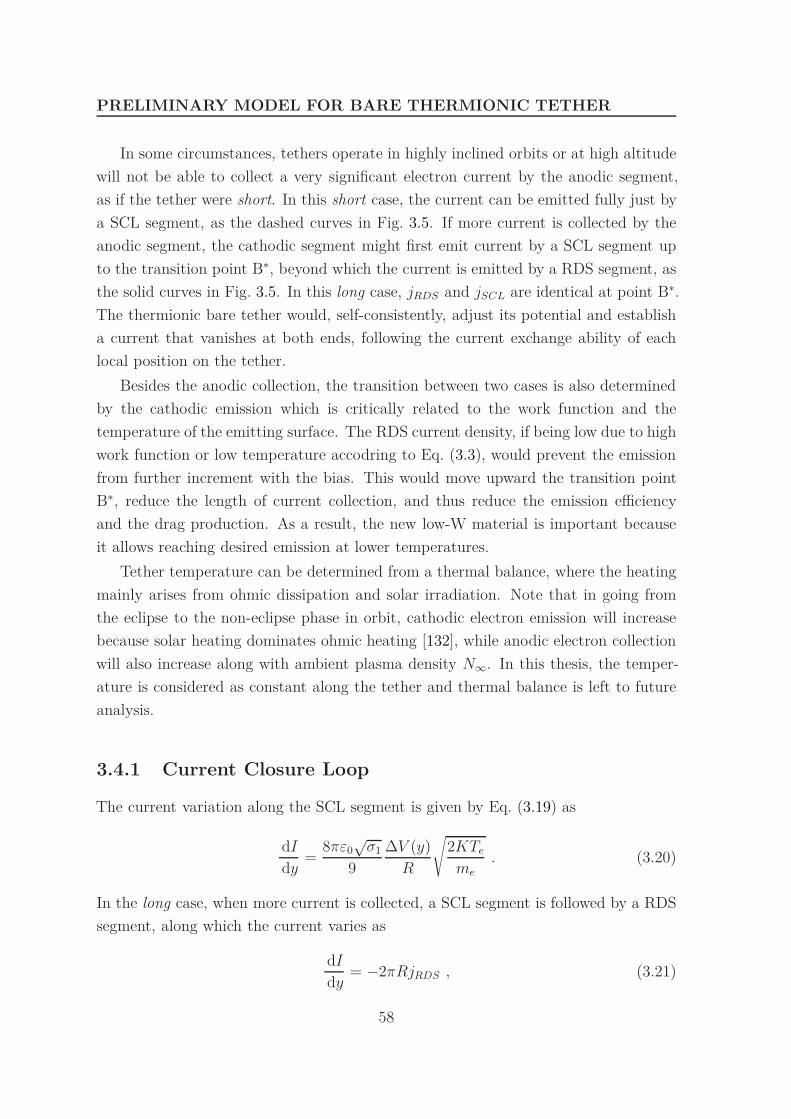
PRELIMINARY MODEL FOR BARE THERMIONIC TETHER
In some circumstances, tethers operate in highly inclined orbits or at high altitude
will not be able to collect a very significant electron current by the anodic segment,
as if the tether were short. In this short case, the current can be emitted fully just by
a SCL segment, as the dashed curves in Fig. 3.5. If more current is collected by the
anodic segment, the cathodic segment might first emit current by a SCL segment up
to the transition point B∗, beyond which the current is emitted by a RDS segment, as
the solid curves in Fig. 3.5. In this long case, jRDS and jSCL are identical at point B∗.
The thermionic bare tether would, self-consistently, adjust its potential and establish
a current that vanishes at both ends, following the current exchange ability of each
local position on the tether.
Besides the anodic collection, the transition between two cases is also determined
by the cathodic emission which is critically related to the work function and the
temperature of the emitting surface. The RDS current density, if being low due to high
work function or low temperature accodring to Eq. (3.3), would prevent the emission
from further increment with the bias. This would move upward the transition point
B∗, reduce the length of current collection, and thus reduce the emission efficiency
and the drag production. As a result, the new low-W material is important because
it allows reaching desired emission at lower temperatures.
Tether temperature can be determined from a thermal balance, where the heating
mainly arises from ohmic dissipation and solar irradiation. Note that in going from
the eclipse to the non-eclipse phase in orbit, cathodic electron emission will increase
because solar heating dominates ohmic heating [132], while anodic electron collection
will also increase along with ambient plasma density N∞. In this thesis, the temper-
ature is considered as constant along the tether and thermal balance is left to future
analysis.
3.4.1 Current Closure Loop
The current variation along the SCL segment is given by Eq. (3.19) as
dI
dy=
8πε0√
σ1
9
∆V (y)
R
√2KTe
me. (3.20)
In the long case, when more current is collected, a SCL segment is followed by a RDS
segment, along which the current varies as
dI
dy= −2πRjRDS , (3.21)
58

3.4 Preliminary Study on Bare Thermionic Tether
where jRDS is given by Eq. 3.3. Using the dimensionless variables as those in Eq. (2.74),
ξ ≡ y
L∗, i ≡ I
I∗, φ ≡ ∆V
EmL∗, (3.22)
the current equations become
di
dξ= ks
2φ < 0 for SCL segment, (3.23)
di
dξ= −kt < 0 for RDS segment. (3.24)
The two dimensionless parameters ks and kt are defined as
ks ≡ 2L∗
3R
(2ε0
Rσc
)1/2 (2KTeσ1
me
)1/4
, (3.25)
kt ≡ 2jRDSL∗
σcREm
, (3.26)
to gauge the SCL emission and the RDS emission respectively. The potential varies
along the cathodic segment asdφ
dξ= i − 1 , (3.27)
which is the same as Eq. (2.78b) for anodic segment.
The circuit equations for anodic segment have been presented in Sec. 2.3.1. Given
by Eqs. (2.84), we have the current at B and the anodic-segment length as
iB = 1 −√
1 − φA3/2 , (3.28a)
ξB =∫ φA
0(1 − φA
3/2 + φ3/2)−1/2 dφ , (3.28b)
which will be used as boundary conditions for the the integrations along the cathodic
segment.
3.4.2 The Short Case B - C
In the short case, Eqs. (3.23) and (3.27) hold all the way to the cathodic end C. The
tip values at the two ends of BC segment are
ξ = ξB : i = iB , φ = 0 , (3.29)
ξ = ξC : i = 0 , φ = φC . (3.30)
59

PRELIMINARY MODEL FOR BARE THERMIONIC TETHER
From Eqs. (3.23) and (3.27), an immediate first integral of (i − 1) di = ks2φ dφ gives
i2 − 2i − ks2φ2 = const. , (3.31)
where the constant can be found by using Eqs. (3.28a), (3.29) and (3.30), yielding
i2 − 2i − ks2φ2 = iB
2 − 2iB = −φA3/2 = ks
2φC2 . (3.32)
From this equation, we acquire φC and the current profile at the SCL segment:
φC = −φA3/4
ks, (3.33)
i = 1 −√
1 − φA3/2 + ks
2φ2 . (3.34)
Substituting Eq. (3.34) into Eq. (3.27), and integrating from Eq. (3.29), the bias
profile at the SCL segment can be written in a reverse way as
ξ = ξB +1
ksarcsinh
−ksφ√
1 − φA3/2
, (3.35)
where ξB is given by Eq. (3.28b). The tether length can thus be associated to φA as
L
L∗≡ ξC = ξB(φA) +
1
ksarcsinh
φA
3/4
√1 − φA
3/2
. (3.36)
This equation shows that φA is a function of L, φA = f(L). So, to discuss the depen-
dence of current emission/collection on φA is equivalent to discuss the dependence on
L.
In the case of dominant ohmic effects, to collect a current as large as the short-
circuit value, iB → 1 and φA → 1, it requires the tether to have infinite length, as
ξC → ∞ given by Eq. (3.36). Using Eq. (2.87), the average current in the short case
is
iav = 1 − φA3/4/ks + φA
ξC. (3.37)
Finally, in the short case, when the current is limited by dominant ohmic effects, the
cathodic-segment magnitudes tend to their limits as
limiB→1
ξBC ≡ limiB→1
(ξC − ξB) = ∞ , limiB→1
φC = − 1
ks
, limiB→1
iav = 1 . (3.38)
60

3.4 Preliminary Study on Bare Thermionic Tether
3.4.3 The Long Case B - B* - C
In the long case, the cathodic-segment emission switches from SCL current to RDS
current at B∗. Thus, equalizing the RHS of Eq. (3.23) and Eq. (3.24), one has the bias
at B∗,
φB∗ = − kt
ks2 . (3.39)
The current and bias profiles along this SCL segment BB∗ are the same as those
described by Eq. (3.34) and Eq. (3.35). Then the SCL-segment magnitudes can now
be written down in terms of φA as
iB∗ = 1 −√
1 − φA3/2 + (kt/ks)
2 , (3.40)
ξB∗ = ξB +1
ksarcsinh
kt/ks√
1 − φA3/2
. (3.41)
At the two ends of the RDS segment B∗C, the tip values are
ξ = ξB∗ : i = iB∗ , φ = φB∗ , (3.42)
ξ = ξC : i = 0 , φ = φC , (3.43)
Along the B∗C segment, given by Eqs. (3.24) and (3.27), an immediate first integral
of (i − 1) di = −kt dφ gives
i2 − 2i + 2ktφ = const. , (3.44)
where the constant can be found by using Eqs. (3.39), (3.40) and (3.42), yielding
i2 − 2i + 2ktφ =kt
ks− φA
3/2 . (3.45)
Then we have the current profile as
i = 1 −√
1 − φA3/2 − (kt/ks)
2 − 2ktφ . (3.46)
Substituting Eq. (3.46) into Eq. (3.27), and integrating from Eq. (3.42), the bias
profile at the RDS segment can be written in a reverse way as
ξ = ξB∗ − 1
kt
√1 − φA
3/2 + (kt/ks)2 +
1
kt
√1 − φA
3/2 − (kt/ks)2 − 2ktφ . (3.47)
61

PRELIMINARY MODEL FOR BARE THERMIONIC TETHER
where ξB∗ is given by Eq. (3.41). Given by Eqs. (3.46) and (3.47), the overall length
of the tether ξC and the cathodic end bias φC become
ξC = ξB∗ − 1
kt
√1 − φA
3/2 + (kt/ks)2 +
1
kt
, (3.48)
φC = −φA3/2
2kt− kt
2ks2 . (3.49)
Again, in the case of dominant ohmic effects, to collect a current as large as the
short-circuit value, iB → 1 and φA → 1, it requires the tether to have infinite length,
as ξC → ∞, due to the infinite SCL-segment length given by Eq. (3.36). The average
current, using Eq. (2.87), then becomes
iav = 1 −(
φA3/2
2kt
+kt
2ks2 + φA
)/ξC . (3.50)
Finally, in the long case, when the current is limited by dominant ohmic effects, the
cathodic-segment magnitudes tend to their limits as:
limiB→1
ξBB∗ = ∞ , limiB→1
ξB∗C = − 1
ks+
1
kt, lim
iB→1φC = − 1
2kt− kt
2ks2 , lim
iB→1iav = 1 .
(3.51)
3.4.4 The Short/Long Cathodic-Segment Transition
If kt > ks, the maximum RDS segment length limiB→1 ξB∗C is negative as shown in
Eq. (3.51). This invalidity of a RDS segment length suggests that , under condition
kt > ks, the tether would always work in the short case, regardless of the tether length.
If kt < ks, there must be a transition tether length Ltr, within which the tether
would fall in the short case, otherwise the long case. For the long case, there must
be φC < φB∗ since the probe-to-plasma bias decreases from the anodic end to the
cathodic end as in Eq. (3.27) and Fig. 3.5. Given by Eqs. (3.49) and (3.39), we have
the condition for a bare tether to work in the long case,
φA ≥ (kt/ks)4/3 , (3.52)
where the value of kt/ks, as found from Eqs. (3.25) and (3.26), reads
kt/ks =3j0
Emσc
(Rσc
2ε0
)1/2 ( me
2kTeσ1
)1/4
. (3.53)
62

3.4 Preliminary Study on Bare Thermionic Tether
Table 3.1 The short/long cathodic-segment transition.
Conditions Case
kt/ks > 1, any L Shortkt/ks < 1, L < Ltr Shortkt/ks < 1, L > Ltr Long
Substituting φA = (kt/ks)4/3 into Eq. (3.36), with ξB(φA) given in Eq. (3.28b), the
shortest length for a tether to work in the long case is given as
Ltr = L∗ ×∫ (kt/ks)4/3
0
[1 − (kt/ks)
2 + φ3/2]
−1/2dφ
+1
ksarcsinh
kt/ks√
1 − (kt/ks)2
. (3.54)
As a conclusion, the conditions of the short/long cathodic-segment transition is shown
in Table 3.1.
3.4.5 Discussion
Let us discuss the results with some typical data in space: σc ≃ 3 × 10⁷S m−1 for
aluminium, kTe ≈ kTi ≈ 0.1eV, a low day density N∞ ≈ 3 × 10¹¹m−3, R = λD ≈4.29mm and σ1 ≈ 0.24. Since there is still not sufficient study on the value of λR for the
electride C12A7 : e−, we will use theoretic value AG = AR for jRDS in Eq. (3.3). The
conductivity of the aluminum tether would remain unchanged with this thin coating.
For a vertical tether in LEO equatorial orbit and a non-tilted centered magnetic dipole
model, a typical motional field lying along the tether reads Em = (vt − Vpl)B ≈7.5km s−1 × 2000T = 150V km−1. A tentative daytime temperature for the tether
T = 300K is used. Different values of work function - 0.6eV, 0.65eV, 0.7eV - are
considered for the C12A7 : e− coating. We then have L∗ = 17.94km and ks = 9.18,
both independent of W . The Lorentz force exerted on the tether, calculated as F =∫
BI dy = BLiavI∗, is shown in Table 3.2 for different values of tether length.
For W = 0.6eV, one has kt = 14.35 > ks and the tether always works in the short
case regardless of tether length (Fig. 3.6a). A slight increase in the work function, say
W = 0.65eV (Fig. 3.6b) or W = 0.7eV (Fig. 3.6c), however results in kt = 2.07 < ks
and a transition in tether length beyond which the tether works in the long case
Ltr = 2.96km (ξCtr = Ltr/L∗ = 0.16), or kt = 0.52 < ks and Ltr = 0.25km (ξCtr =
63

PRELIMINARY MODEL FOR BARE THERMIONIC TETHER
Table 3.2 Lorentz force generated by a thermionic bare tether.
1 km 5 km 10 km 20 km
0.6 eV 0.02 N 1.1 N 5.8 N 29.5 N0.65 eV 0.02 N 1.0 N 5.5 N 26.7 N0.7 eV 0.01 N 0.6 N 2.6 N 11.8 N
ΦA
iB
iav
IΞC- ΞBM ΞC
ΦC1 2 3 4
ΞC
-0.2
0.2
0.4
0.6
0.8
1.0
(a)
IΞC -ΞBM ΞC
ΦA
iB
iav
ΦC
1 2 3 4 5ΞC
-0.2
0.2
0.4
0.6
0.8
1.0
(b)
ΦA iB
iavIΞC -ΞBM ΞC
ΦC
2 4 6 8ΞC
-1.5
-1.0
-0.5
0.5
1.0
(c)
Fig. 3.6 Anodic bias φA, collected current iB, cathodic-to-total length ratio (ξC−ξB)/ξC
, cathodic bias φC , and length-averaged current iav are plotted against tether lengthξC , at the value ks = 9.18, with different work functions: (a) W = 0.6eV, kt = 14.35,no ξCtr; (b) W = 0.65eV, kt = 2.07, ξCtr = 0.35; (c) W = 0.7eV, kt = 0.52, ξCtr = 0.08.
64

3.4 Preliminary Study on Bare Thermionic Tether
0.014). The short/long cathodic-segment transition is sensitive to the work function.
This is because the work function influences the transition conditions in Table 3.1
and the transition length in Eq. (3.54) through the ratio kt/ks - the greater the ratio
is, the greater the value of Ltr is, or even there is not a transition length for long
case to be present - and the ratio kt/ks [see Eq. (3.53)] is proportional to jRDS and
thus proportional to the exponential term exp (−W/kT ), being sensitive to the work
function.
Shown in Figs. 3.6a and 3.6b for W = 0.6eV and W = 0.65eV respectively, the
cathodic-to-total length ratio (L − LB)/L first decreases rapidly with the increase of
the total tether length down to around 15%, which is indeed small and implies quick
current emission from a short segment at the cathodic end of the tether. However, as
mentioned, the current emission efficiency is very sensitive to the work function of the
material as the work function determines critically the RDS current density. Shown
in Fig. 3.6c for W = 0.7eV, the cathodic segment is around 50% of total length, and,
for a given tether total length, the average current is reduced significantly compared
to the results for the other two values of work functions.
If the tether length is further increased, L ≫ L∗, the tether falls into the case of
dominant ohmic effects, iB ≈ 1, and the cathodic-to-total length ratio is increased
(Fig. 3.6) because the SCL segment length keeps increasing while the OML segment
length is limited. The cathodic bias |φC| is limited to 1/ks for W = 0.6eV as in the
short case or limited to (1/2kt)+kt/2ks2 for W = 0.65eV as in the long case, both being
much smaller than φA as shown in Figs. 3.6a and 3.6b. As a result, the plasma and
tether potential lines move close to each other, covering most of the cathodic segment,
and the current decreases to zero rapidly at the short end of the tether. Thus a long
segment possessing the near short-circuit current implies an efficient current emission
in the case of dominant ohmic effects. Again, for W = 0.7eV, |φC| increases to a value
larger than φA (Fig. 3.6c), as opposite lower W values, which prevents the cathodic
segment from possessing a long section with the short-circuit current and thus the
current emission is much less efficient, however still begin much efficient than ion
collection at the cathodic segment.
We have considered a round-wire radius R = λD ≈ Rmax throughout for simplicity;
with Rmax near λD independent of bias for Ti = Te, we then have rsh as given by
Eq. (3.18) with σ1 ≈ 0.24 and R = λD. This results in too heavy tethers. For
R = 4.3mm, an aluminum wire just 1 km long would be 157 kg heavy. In the case of
a sensible radius well below λD one must use a more complex sheath-radius law given
in [43, 124]. Alternatively, one can consider a tether of thin-tape cross section and
65

PRELIMINARY MODEL FOR BARE THERMIONIC TETHER
width w. Round-wire OML results hold for tapes with perimeter 2w replacing 2πR
or w = πR. Further, the maximum width for OML current to hold is wmax = 4Rmax
[128]. A tape 0.1 mm thick and 15 mm wide say, roughly satisfying the above, would
only be around 4 kg heavy for 1 km length. The detailed dependence of SCL current
on the electron emitter being cylindrical, through the β(rsh/r0) function, was lost for
rsh > 10r0 (β = 1), as represented by Eq. (3.12a).
As regards geomagnetic-field effects, the Parker-Murphy 2D canonical upper-bound
on current lies well above the OML current if the ratio of tether radius to electron
thermal gyroradius R/le is small. Detailed analysis shows that both (R/le)2 and
(R/λD)2 must be small for such effects to be negligible [128]. In turn, effects of the
magnetic field generated by the tether current itself, prove negligible for thin-tape
tethers because ohmic effects then limit the current in the tether [74, 129].
Due to the tether-to-plasma relative flow there will be differences in upstream
and downstream structures, as there are also differences in sheath structures around
round and thin-tape tethers at rest in the plasma [128]. This need not have an effect
in collected current, however. In Ref. [78] it was shown that the 2D OML current
law does not depend on azimuthal symmetry; it just requires that i) the undisturbed
velocity distribution of the attracted species is isotropic, and ii) all orbits traced back
in time from the probe reach infinity (there may be no potential barrier for the probe
surface). For the no-flow case condition ii) holds for a round tether with radius below
Rmax. Condition i) is clearly satisfied for the anodic segment, where electrons are
the attracted particles. As regards the cathodic segment, the collected ion current is
negligible against the emitted electron current, and only the simplest description was
needed.
A basic issue arises, however, from the mesothermal character of the relative flow,
which results in the density of ions exceeding N∞ where rammed back (upstream),
and in electron density lying below N∞ everywhere [78], breaking quasineutrality in a
large upstream region. It has been suggested that a fundamental plasma phenomenon,
adiabatic electron trapping [57], might resolve this paradox [104, 125]. Current collec-
tion by positively polarized cylindrical Langmuir probes immersed in flowing plasmas
is analyzed using a non-stationary direct Vlasov-Poisson code, which confirmed that
electron trapping at the probes front side occurs [118, 120].
66

Chapter 4
ASYMPTOTIC ANALYSIS ON
THE SHEATH
The first model presented in Chap. 3, based on Langmuir’s SCL current and the OML
ion collection sheath, provides a simple and fast derivation for tether-plasma current
exchange, which can be implemented into tethered-system flight simulators. However
it is still a crude model, without giving details of the sheath formation. In this chapter,
this problem will be analyzed in detail using asymptotic method. The main content
of this chapter has been published in Ref. [21].
The terms sheath [82] and plasma [83] were introduced by Langmuir during 1920s.
Inside the sheath, charged particles can be considered as originating from the sheath
boundary where the electric field is nearly zero. And the current is thus close to
be space-charge-limited and can be approximated by Child-Langmuir formulas as
Eqs. (3.12).
In 1929, Tonks and Langmuir [144] presented a separate treatment of plasma and
sheath. In the quasineutral plasma, the solutions can be simplified if the Laplacion
of the potential in Poisson’s equation is negligible. This gives the quasineutrality
equation in plasma:∑
ρ(Φ) = 0 . (4.1)
At some distance away from the probe, say x1, the derivative of the potential given
by this approximation is found to be infinite. The sheath edge, where the plasma
ends and the sheath begins, can be placed at a location where the quasineutrality
approximation would fail, being some value of x larger than x1.
These two regions are disjoint and it is necessary to introduce other regions to
achieve smooth matching. Considering this transition between layers, current col-
67

ASYMPTOTIC ANALYSIS ON THE SHEATH
lection and sheath structure around a spherical Langmuir probe have been studied
in the literature, using radial-motion theory [5] or orbital-motion theory for mono-
energetic attracted species [1, 11, 79], while the cylindrical case was investigated for
a Maxwellian distribution [43, 76, 124, 128]. The impact of relativistic effects using
similar methods has been analyzed for a possible Jupiter mission with electrodynamic
bare tethers [17, 122].
In presence of emission, considering both emitted electrons and collected ions, the
sheath formation was first investigated by Langmuir for a planar sheath [84]. Fluid
models have then been often used in the literature to analyze planar [35, 59, 109],
cylindrical [50] or spherical [150] sheath structures. Following orbital-motion theory,
Chang and Bienkowski discussed the electron emission effects in front of spherical
and cylindrical probes, considering their kinetics and the attracted species as mono-
energetic [16].
Due to the cylindrical geometry, it is difficult to find an easy analytic solution of
Poisson’s equation considering both electrons and ions inside sheath, even using fluid
models and considering vanishing electric field at both emitting surface and sheath
edge. To shed light on the sheath formation considering emission, this study would
follow closely the methods in Ref. [128] and extend the orbital-motion-limited (OML)
ion-collection analysis to investigate the probe response due to electrons emitted by
a negatively-biased cylindrical probe. Although electrons would dominate inside the
sheath near or within the SCL regime, ions outside the sheath in the plasma plays an
important role in defining the sheath boundary.
4.1 Electron-Emitting Cylinder
In the presence of emission, emitted electrons result in negative space charge, which
decreases the electric field that accelerates them outwards, or even reverses it, de-
celerating electrons near the emitting probe. In the case of a monotonic potential
as curve c in Fig. 4.1, all electrons are accelerated outwards without meeting any
barrier, corresponding to the emission at any local point on segment B*C (Fig. 3.5).
Locally, the emitted current Iem is as high as the maximum current that can possibly
be emitted by the negatively biased probe, Iem = Iemp, where Iemp is determined by
the Richardson-Dushman (RDS) law, as in Eq. (3.3):
Iemp = 2πRL × AGT 2p exp
(− W
kTp
). (4.2)
68

4.1 Electron-Emitting Cylinder
As |Φp| decreases from tether end C, negative space charge increases its effect, and at
some point B*, the electric field vanishes at the emitting surface (curve b in Fig. 4.1),
which is the onset of the current being SCL. If we draw the potential profile Φ/Φp
versus R2/r2 as that in Fig. 2.6 for the case of no emission, curve b in Fig. 4.2 is
horizontal at the emitting surface R2/r2 = 1. Under further decrease of |Φp| from B*
to zero-bias-point B, a retarding field for electrons develops in front of the emitting
surface as curve a in Fig. 4.1. There is then a local minimum of potential, Φm, at a
radius rm > R, which can be considered as a virtual cathode for the emission after rm.
Inside this virtual cathode, it is a potential hill for electrons to climb. The electrons
that are not energetic enough would be repelled back to the emitter, the current being
Iem < Iemp. In Fig. 4.2, curve a would then actually exceed the full square frame.
Φ
r
c, Iem = Iemp, RDS
a, Iem < Iemp, SCL
b, Iem = Iemp, B∗
a
cbΦm
R rm
Fig. 4.1 Typical potential distributions of a negatively biased probe with electronemission. Iem is the electron current successfully emitted by the probe. Iemp is thecurrent that can be emitted by the probe if it is not saturated by the probe bias.
1
0 1
|Φp|Φ/Φp
R2/r2
ab
c
Fig. 4.2 Schematics of potential profile Φ/Φp versus R2/r2 for given emission withdifferent bias values, under condition R = Rmax for ion OML collection.
69

ASYMPTOTIC ANALYSIS ON THE SHEATH
250 300 35010
−10
10−8
10−6
10−4
10−2
100
102
104
T (K)
Curr
ent D
ensity (
A/m
2)
250 300 35010
4
106
108
1010
1012
1014
1016
1018
T (K)
Num
ber
Density (
1/m
3)
W=0.6 eV
W=0.7 eV
W=0.8 eV
W=0.9 eV
W=1.0 eV
Fig. 4.3 Richardson-Dushman current density and emitted particle density versusprobe temperature for different work function of the emitting material.
In this chapter, we concentrate on the monotonic potential case, corresponding to
the segment B∗C in Fig. 3.5. Under assumptions of high bias and relatively low emis-
sion, emitted electrons are accelerated across the sheath, presenting a small amount
of space charge in the quasineutral region far away from the probe. Outside but
close to the sheath, the behavior of the potential profile would be similar to that of
non-emitting OML ion collection, with modifications arising from the space charge of
emitted electrons, in particular on the two transitional layers that match the quasineu-
tral and sheath regions. For simplicity, we consider throughout R = Rmax cases, where
potential profile curves in Fig. 4.2 are tangent to the diagonal at some radius r in the
quasineutral plasma. Considering equal plasma electron-ion temperature Te = Ti = T ,
we look for the general parametric dependence of Rmax and locate the probe bias where
the current starts to be SCL (curve b in Figs. 4.2 and 4.1).
4.1.1 Particle Densities
Electrons are emitted at the probe with a half-Maxwellian velocity distribution [16,
115],
f 1
2M(vr, vθ) =
Nempme
πKTpexp
(−mevr
2/2 + mevθ2/2
KTp
). (4.3)
70

4.1 Electron-Emitting Cylinder
Given by this distribution, the emitted electron density Nemp can be associated with
Iemp as
Nemp =Iemp/2πRL
e√
2KTp/πme
, (4.4)
where L is the length of the probe. The emitted current density and particle density
versus probe temperature for different work function are shown in Fig. 4.3. The Vlasov
equation conserves the distribution function along electron orbits. Since we consider
the case of monotonic potential, vθ decreases as angular momentum
Je = mervθ (4.5)
keeps constant while moving outwards. Radial velocity thus increases, as energy
Ee = mev2r/2 + mev
2θ/2 − e∆Φ , ∆Φ = Φ − Φp , (4.6)
keeps constant, vθ decreases, and Φ increases. As a result, there is not any potential
barrier and all electrons emitted at the probe can reach infinity and are thus present
at any r. For electrons with energy Ee, the integration domain of Je is thus
0 ≤ J2e ≤ J2
eR(Ee) = 2meR2Ee , (4.7)
where we defined J2er(Ee) = 2mer
2(Ee + e∆Φ). The velocity distribution integration
becomes
Nem(r)
Nemp= 2
∫∞
0
exp(−Ee/KTp)
πKTp× arcsin
√√√√ R2Ee
r2(Ee + e∆Φ)dEe . (4.8)
Taylor expansion of arcsin√
a2x/(x + 1) around x → 0 is arcsin√
a2x/(x + 1) =
a(√
x + O[x]3/2). Under condition of e∆Φ/KTp ≫ 1, we have
arcsin
√√√√ R2Ee
r2(Ee + e∆Φ)=
R
r
√Ee
e∆Φ+ O
([Ee
e∆Φ
]3/2) . (4.9)
The emitted electron density becomes
Nem(r)
Nemp≈ R
r
√KTp
πe(Φ − Φp), (4.10)
71

ASYMPTOTIC ANALYSIS ON THE SHEATH
which corresponds to radial motion away from the probe. This approximation has an
error of the order of (KTp/e∆Φ)3/2, breaking down near the probe surface where the
error becomes infinite. However, the conditions of high bias and low probe tempera-
ture (low energy of emitted electrons) confine the failure of this approximation to the
vicinity of the probe.
As introduced in Sec. 2.2.3, following Eq. (2.57), the ion density at r is given by
Ni(r)
N∞
=∫
∞
0
exp(−E/KT )
πKT
×[2 × arcsin
J∗
r (E)
Jr(E)− arcsin
J∗
R(E)
Jr(E)
]dE , (4.11)
with Jr(E) =√
2mir2(E − eΦ) ≥ 0 and J∗
R(E) = JR(E) if R ≤ Rmax. For |eΦp|/kTe
values of interest here, the density of repelled plasma electrons is given by the simple
Boltzmann law,Ne(r)
N∞
= exp
(eΦ
KTe
). (4.12)
4.1.2 Qualitatively Description of the Solution
Probe1
R2/r20 1
UndisturbedPlasma
Forbidden domainif OML regime
0
1
2
Φ/Φp
Fig. 4.4 Schematic potential profile for R = Rmax. The plasma is quasineutral belowpoint 1. There is no barriers J∗
r = Jr below point 0. Around point 1 and 2 there aretwo transitional layers to match the plasma solution and the sheath solution.
To determine J∗
r (E), it requires information of the potential everywhere. However,
if the solution is divided into several layers while integrating from infinity to the
probe, inside each layer,the RHS of Poisson’s equation can be simplified to involve
72

4.1 Electron-Emitting Cylinder
only information at r [79, 128]. From infinity moving inwards, quasineutrality and the
no barrier condition J∗
r (E) = Jr(E) holds until point 0 that is determined by
d (r2Φ)
dr
∣∣∣∣∣∣r0
= 0 . (4.13)
Under condition R = Rmax, we have r20Φ0 = R2Φp. Further inwards, the plasma
quasineutral approximation results in infinity derivative as dΦ/ dr → ∞ at point 1
(Fig. 4.4). One transitional layer at the vicinity of point 1 brings the solution to point
2 a bit close to the probe, where Ψ diverges and another transitional layer is required.
These two transitional layers, both very thin, can smoothly match the plasma solution
for r > r1 and the sheath solution for r < r2 ≈ r1.
4.1.3 Normalization
We introduce normalized parameters as
ξD ≡ R
λD, ν ≡ Nemp
N∞
, θ ≡ T
Tp, (4.14)
where T = Ti ≈ Te, λD =√
ǫ0KT/N∞e2, and N∞ is the plasma density at infinity.
Energy and angular momentums of ions are also normalized as
ǫ ≡ E
KT, j =
J√2miR2KT
, j2z (ǫ) ≡ J2
r
2miR2KT= z2(ǫ + Ψ) . (4.15)
The r dependent variables in Poissons’s equation are defined as
z ≡ r
R, Ψ(z) ≡ −eΦ(r)
KT> 0 , ni,e(z) ≡ Ni,e(r)
N∞
, nem(z) ≡ Nem(r)
Nemp. (4.16)
Then Poisson’s equation becomes
1
ξ2Dz
d
dz
(z
dΨ
dz
)= ni − ne − νnem , (4.17)
Ψ(1) = Ψp > 0 , Ψ(∞) → 0 , (4.18)
73
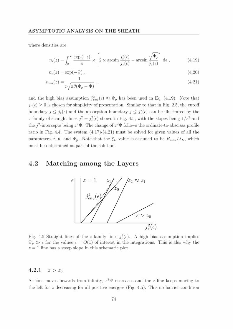
ASYMPTOTIC ANALYSIS ON THE SHEATH
where densities are
ni(z) =∫
∞
0
exp (−ǫ)
π×
2 × arcsinj∗
z (ǫ)
jz(ǫ)− arcsin
√Ψp
jz(ǫ)
dǫ , (4.19)
ne(z) = exp(−Ψ) , (4.20)
nem(z) =1
z√
πθ(Ψp − Ψ), (4.21)
and the high bias assumption j2z=1(ǫ) ≈ Ψp has been used in Eq. (4.19). Note that
jr(ǫ) ≥ 0 is chosen for simplicity of presentation. Similar to that in Fig. 2.5, the cutoff
boundary j ≤ jz(ǫ) and the absorption boundary j ≤ j∗
z (ǫ) can be illustrated by the
z-family of straight lines j2 = j2z (ǫ) shown in Fig. 4.5, with the slopes being 1/z2 and
the j2-intercepts being z2Ψ. The change of z2Ψ follows the ordinate-to-abscissa profile
ratio in Fig. 4.4. The system (4.17)-(4.21) must be solved for given values of all the
parameters ν, θ, and Ψp. Note that the ξD value is assumed to be Rmax/λD, which
must be determined as part of the solution.
4.2 Matching among the Layers
j2z(ǫ)
ǫ z = 1
z0
z > z0
z1
j2env
(ǫ)
z2 ≈ z1
Fig. 4.5 Straight lines of the z-family lines j2z (ǫ). A high bias assumption implies
Ψp ≫ ǫ for the values ǫ = O(1) of interest in the integrations. This is also why thez = 1 line has a steep slope in this schematic plot.
4.2.1 z > z0
As ions moves inwards from infinity, z2Ψ decreases and the z-line keeps moving to
the left for z decreasing for all positive energies (Fig. 4.5). This no barrier condition
74

4.2 Matching among the Layers
j∗
z (ǫ) = jz(ǫ) holds until z0, where z2Ψ starts to increase. If R = Rmax, z0 lies on
the diagonal in Fig. 4.2, giving z20Ψ0 = Ψp. For z > z0, the ion density in Eq. (4.19)
becomes
ni(z) = 1 −∫
∞
0
exp(−ǫ)
πarcsin
√Ψp
j2z (ǫ)
dǫ . (4.22)
And, due to Ψ ≪ Ψp in this region, the emitted electron density in Eq. (4.21) can be
further approximated as
nem(z) ≈ 1
z√
πθΨp
. (4.23)
Then the potential Ψ(z) for any z ≥ z0 is given by solving the quasineutrality equation
1 −∫
∞
0
exp(−ǫ)
πarcsin
√Ψp
j2z (ǫ)
dǫ − exp(−Ψ) − ν
z√
πθΨp
= 0 . (4.24)
We can thus determine z0 and Ψ0 by conditions
1 + exp (Ψ0) erfc(√
Ψ0
)= 2 exp(−Ψ0) +
2ν
Ψp
√Ψ0
πθ, (4.25)
Ψ0 = Ψp/z20 . (4.26)
Because Eq. (4.22) is valid as long as R ≤ Rmax, the potential profile for z > z0
calculated from Eq. (4.24) is also valid for R ≤ Rmax, being function of ν, θ and Ψp
only, independent of R. However, we know that, as R changes, the location of z0
changes. This implies that Eq. (4.24) does not result in d (z2Ψ) / dz = 0 at z0, which
is the accurate definition of z0. Therefore, the position of z0 can not arise from this
approximated quasineutrality solution directly. In this study, we impose the condition
R = Rmax and z20Ψ0 = Ψp, acquiring z0 and Ψ0 by Eqs. (4.25) and (4.26) before
the global sheath solution is found. Then looking for the Rmax value that provides a
consistent solution does require a jump of d (z2Ψ) / dz at z0. However, using locally
the full Poisson’s equation Eq. (4.17) around z0 and Eqs. (4.19), (4.20) and (4.23)
for particle densities can round the profile at z0, with no effect beyond its immediate
neighbourhood [128].
4.2.2 z1 < z < z0
From z0 inwards, the quasineutral condition holds until it breaks down near some
radius z1 where dΨ/ dz|z=z1is found to diverge. In this layer, the no-barrier condition
does fail, j∗
z (ǫ) 6= jz(ǫ), because z2Ψ starts to increase.
75
ASYMPTOTIC ANALYSIS ON THE SHEATH
In the ǫj-plane, as z decreases, both the slopes of z-lines and the j2-incepts increase.
The z-lines in this layer move to the right with increasing slopes, thus forming a concave
envelope, as the dashed curve in Fig. 4.5, which is determined by
j2 − j2z (ǫ) = 0 ,
∂ [j2 − j2z (ǫ)]
∂z= 0 . (4.27)
These two equations lead to the parametric representation for the envelope
ǫenv (z) = −z dΨ
2 dz− Ψ , j2
env(z) = −z3 dΨ
dz. (4.28)
All the z-lines osculate with this envelope at [ǫenv(z), j2env(z)] and the absorption bound-
ary j∗
z (ǫ) is thus given by
j∗
z (ǫ) = jenv(ǫ), for ǫ < ǫenv(z)
= jz(ǫ), for ǫ ≥ ǫenv(z) . (4.29)
As shown in Eq. (4.28), the knowledge of Ψ(z) itself is required to determine the
envelope. We approximate this envelope by a hyperbola that is tangent to the z0 line
at ǫ = 0 and j2z = z2
0Φ0, and limited by the z1-line as the asymptote for ǫ → ∞ [128],
j2env(ǫ) = j2
z1(ǫ) − (z2
1Ψ1 − z20Ψ0)
2
z21Ψ1 − z2
0Ψ0 + (z20 − z2
1)ǫ. (4.30)
Use of Eq. (4.30), however, requires values for z1 and Ψ1 which are still unknown.
Near z1, we have j∗
z (ǫ) ≈ jenv(ǫ), and thus the ion density becomes
ni(z) =∫
∞
0
exp (−ǫ)
π×
2 × arcsinjenv(ǫ)
jz(ǫ)− arcsin
√Ψp
jz(ǫ)
dǫ . (4.31)
Use of Eq. (4.31) for quasineutrality at z1 provides a first relation for z1 and Ψ1.
If we write the quasineutrality equation as f(z, Ψ) = 0, the implicit function theorem
gives df/ dΨ = ∂f/∂Ψ+∂f/∂z · dz/ dΨ = 0. Another relation thus arises from using
the equivalence of the divergent condition dz/ dΨ = 0 at z1, rewritten as
∂ni(z)
∂Ψ
∣∣∣∣∣∣z1
− ∂ne(z)
∂Ψ
∣∣∣∣∣∣z1
− ∂nem(z)
∂Ψ
∣∣∣∣∣∣z1
= 0 , (4.32)
76

4.2 Matching among the Layers
where ∂nem(z)/∂Ψ|z1actually vanishes. Thus z1 and Ψ1 can be found from equations
∫∞
0
exp (−ǫ)
π×
2 × arcsinjenv(ǫ)
jz1(ǫ)
− arcsin
√Ψp
jz1(ǫ)
dǫ
− exp(−Ψ1) − ν
z1
√πθΨp
= 0 , (4.33)
∫∞
0
exp (−ǫ)
2π(ǫ + Ψ1)×2
√√√√ j2env(ǫ)
j2z1
(ǫ) − j2env(ǫ)
−√√√√ Ψp
j2z1
(ǫ) − (ǫ + Ψp)
dǫ
− exp(−Ψ1) = 0 . (4.34)
The mathematical definition of the envelope in Eq. (4.27) gives that dj2env(ǫ)/ dǫ|ǫenv =
dj2z (ǫ)/ dǫ|ǫenv = z2. Together with the approximated envelope in Eq. (4.30), ǫenv(z) is
given by
ǫenv(z) =
√(z2
1Ψ1 − z20Ψ0)
2(z20 − z2
1)
z2 − z21
− (z21Ψ1 − z2
0Ψ0)
z20 − z2
1
. (4.35)
From the parametric presentation of the envelope Eq. (4.28), the potential is obtained
as
Ψ(z) =j2
env(ǫenv)
z2− ǫenv . (4.36)
Note that, once the potential profile is determined throughout this layer, the resultant
overall particle density ni − ne − νnem can be used to evaluate the error of Eq. (4.30)
as jenv(ǫ) approximation. The maximum error evaluated for values θ = 4, ν = 0, 20,
50, 70, and 100 is found of the order of 1% or less, validating that approximation.
4.2.3 First Transitional Layer around z1
From z1 inwards, because of the sharp increase in Ψ, quasineutrality breaks down. A
very thin transitional layer, in the vicinity of z1, takes the solution to a radius z2 a bit
closer to the probe, where Ψ, rather than dΨ/ dz, is found to actually diverge.
The j-line moves to the right from z1 to z2, keeping nearly parallel as shown in
Fig. 4.5, giving j∗
z (ǫ) ≈ jenv(ǫ) for the values ǫ = O(1) of interest. Thus the ion density
will be same as Eq. (4.31). We can expand the RHS of Poisson’s equation about z1
and Ψ1, to order z1 − z and (Ψ − Ψ1)2, which represents the divergent behavior of
quasineutral potential at z1, Ψ − Ψ1 ∽√
z1 − z, leading [128]
d2Ψ
ξ2D dz2
= µz1 − z
z1+ λ
(Ψ − Ψ1)2
2, (4.37)
77
ASYMPTOTIC ANALYSIS ON THE SHEATH
where the parameters µ and λ are given by
µ =∫
∞
0
exp (−ǫ)
π×
2
√√√√ j2env(ǫ)
j2z1
(ǫ) − j2env(ǫ)
−√√√√ Ψp
j2z1
(ǫ) − (ǫ + Ψp)
dǫ − ν
z1
√πθΨp
,
(4.38)
λ =∫
∞
0
exp (−ǫ)
4π(ǫ + Ψ1)2
2jenv
3j2z1
(ǫ) − 2j2env(ǫ)
[j2
z1(ǫ) − j2
env(ǫ)]3/2
−√
Ψp
3j2z1
(ǫ) − 2(Ψp)[j2
z1(ǫ) − (ǫ + Ψp)
]3/2
dǫ
− exp(−Ψ1) . (4.39)
After defining
z1 − z
z1= βξ ≡
(√2
λµ
1
ξ2Dz2
1
)2/5
ξ ,
Ψ − Ψ1 ≡√
2µβ
λY , (4.40)
Poisson’s equation becomes the first Painleve transcendent [10] with initial condition
that matches smoothly the quasineutrality solution from z1 outwards,
d2Y
dξ2= Y 2 + ξ , lim
ξ→−∞
−Y =√
−ξ . (4.41)
For the expansion to be valid in this thin layer, it is required β, given in Eq. (4.39),
to be small.
Integration of Eq. (4.41) shows Y diverging as [79, 128]
Y ≈ 6
(ξ − ξ2)2 , at ξ → ξ2 ≈ 3.42 , (4.42)
which gives the value of z2,
z2 = z1 (1 − βξ2) . (4.43)
As Ψ2 diverges at z2, it is actually left undetermined.
Different from the determination of z0, z1, Ψ0 and Ψ1, the value of z2 can not be
calculated until the entire sheath structure is solved. Because it depends on ξD and ξD
appears in the definition of β given by Eq. (4.40). If ξD is somehow poorly determined,
the same applies to z2.
78

4.2 Matching among the Layers
4.2.4 Second Transitional Layer around z2
A second thin transitional layer around z2 is needed to match the solution inside
the sheath. At this layer, being thin and faraway from the probe under high bias
assumption, space curvature can be ignored in 2D Laplace operator of Poisson’s equa-
tion, equivalently z ≈ z2. However, the complete expression of the RHS of Poisson’s
equation needs to be retained as
d2Ψ
ξ2D dz2
=∫
∞
0
exp (−ǫ)
π
2 × arcsin
√√√√ j2env(ǫ)
z22(ǫ + Ψ)
− arcsin
√Ψp
z22(ǫ + Ψ)
dǫ
− ν
z2
√πθΨp
, (4.44)
where the ambient electrons density has been neglected. To match the first transitional
layer, we have the behavior of the potential from z2 outwards as
Ψ =12
λξ2D(z1 − z1βξ2 − z)2
+ Ψ1 . (4.45)
From z2 inwards, the sharp increase of Ψ results in jz(ǫ) ≫ jenv(ǫ) and z22Ψ ≫ ǫ for
the values ǫ = O(1) of interest, thus giving the ion density as
ni =κ
πz2
√Ψp
Ψ, (4.46)
where κ is
κ =∫
∞
0
2 exp(−ǫ)jenv(ǫ)√
Ψp
dǫ − 1 . (4.47)
Poisson’s equation becomes
d2Ψ
ξ2D dz2
=κ
πz2
√Ψp
Ψ− ν
z2
√πθΨp
. (4.48)
After changing variables
g = gpΨ
Ψp, gp =
(πΨp
κz2ξ2D
)2/3
, u = lnz2
z, (4.49)
we haved2g
du2=
1√g
− µs√gp
, µs =ν
κ
√π
θΨp, (4.50)
79

ASYMPTOTIC ANALYSIS ON THE SHEATH
where dz ≈ z2 du has been used. If µs/√
gp is much smaller than 1/√
g, we can assume
g ≈ g0 + g1, where g1 ≪ g0 is the correction due to small µs/√
gp. Then we have
d2g
du2≈ 1√
g0
− g1
2g3/20
− µs√gp
. (4.51)
After integrating the resultant equations g′′
0 = 1/√
g0 and g′′
1 = −g1/2g3/20 − µs/
√gp,
we find the behavior at the inward tip of the second transitional layer for increasing u
as
g =(
3u
2
)4/3
− 9µs
20√
gp
u2 . (4.52)
This two-term expansion in Eq. (4.52) provides the matching condition for the sheath.
As g becomes large along with u, moving into the sheath, µs/√
gp becomes comparable
to 1/√
g and a different solution for the sheath needs to be found.
4.2.5 Sheath and OML Validity
Inside most of the sheath region, z-lines lie far to the right, leading to jz=1(0) ≪jz(ǫ) ≈ jz(0) and j∗
z (ǫ) = jenv(ǫ) ∼ jz=1(0), the ion density then reading
ni(z) =κ
πz
√Ψp
Ψ, (4.53)
where κ is given by Eq. (4.47). Although this approximation fails near the probe,
as with the approximation Eq. (4.21), the high bias assumption makes space-charge
effects negligible within some neighborhood of the probe. Moreover, in the case of
sufficient electron emission, the ion space charge is small compared to that of the
emitted electrons and thus the error of this approximation can be further neglected.
The plasma electron density can be ignored inside the sheath and the emitted electron
density used is the fluid approximation of Eq. (4.21). We would impose a bound
nem = 1 if nem > 1 in the calculation. Poisson’s equation now becomes
1
zξ2D
(d
dzz
dΨ
dz
)=
κ
πz
√Ψp
Ψ− ν
z√
πθ (Ψp − Ψ). (4.54)
80
4.2 Matching among the Layers
Using same changes of variables as Eq. (4.49) yields Poisson’s equation as
d2g
du2= exp(−u)
(1√g
− µs√gp − g
). (4.55)
To match with the behavior of the potential at the inward tip of the second transitional
layer given by Eq. (4.52), for small u > 0 we have
g =(
3u
2
)4/3
− 9µsu2
20√
gp
, g′ = (12u)1/3 − 9µsu
10√
gp
, (4.56)
where the curvature effect, represented by the factor e−u in Eq. (4.55), was ignored.
Equation (4.55) must be integrated from small u, with the behavior of Eq. (4.56),
till reaching the probe at z = 1, i.e., up = ln z2. Integration depends on the unknown
parameter ξD. For given ν, θ, and Ψp, the corresponding ξDm(ν, θ, Ψp) = Rmax/λD is
determined by a shooting method, till condition g(up) = gp is satisfied,
g [ln z2(ξDm)] =
(πΨp
z2κξ2Dm
)2/3
. (4.57)
For decreasing values of Ψp, the derivative dg/ du at the probe keeps positive until
the SCL condition dg/ du = 0 is reached. The probe potential here, ΨSCL(ν, θ), is the
minimum of Ψp values that allow monotonic potential profile.
Let us discuss the results with some typical data in space, KT = 0.1eV and a
somewhat low day density N∞ = 3×10¹¹m−2. Results are shown for a tentative tether
temperature θ = 4 (Tp ≈ 290.1K) and several emitted electron densities, ν = 20, 50,
70 and 100, corresponding to work function W ≈ 0.708, 0.685, 0.677 and 0.668 eV
respectively.
For different ν values and a range of Ψp values, Figure 4.6 shows Rmax/λD and
dg/ du|z=1, Figure 4.7 shows Ψ0, Ψ1, Ψp/z21 , and Ψp/z2
2 , and Figure 4.8 shows the
parameters β, κ, gp, and µs. The results for the case of no emission (ν = 0) are also
shown in the figures. Except for the ν = 0 case, the curves end at the probe potential
ΨSCL(ν, θ), where SCL condition is met. The values of Rmax/λD in Fig. 4.6 are slightly
different from the value also given in Ref. [128] because of our use of Eq. (4.43) for
z2, instead of a further approximation Ψp/z21 ≈ (1 + 2βξ2)Ψp/z2
2 as in Eq. (A6) of
Ref. [128]. Figure 4.9 shows Ψ/Ψp versus 1/z2 profiles for ν = 100, and Ψp = 5000,
1000 and 300. Because the second transitional layer is not actually solved (only the
solution behavior being found at both layer ends), this layer is not shown in this figure.
81

ASYMPTOTIC ANALYSIS ON THE SHEATH
101
102
103
0.5
1
1.5
2
2.5
3
Ψp
Rmax/λ
D
−→ ν
101
102
103
0
0.5
1
1.5
2
2.5
Ψp
dg/duatprobe
(a)
(b)
−→ ν
ν = 0ν = 20ν = 50ν = 70ν = 100
Fig. 4.6 The maximum radius and the derivative at the probe for θ = 4 and several ν,and for a range of Ψp. Except for the case ν = 0, curves end at the probe potentialwhere the SCL condition is met, being ΨSCL = 26.2, 89.7, 143.0 and 238.8 for ν = 20,50, 70, and 100 respectively.
4.2.6 Effects of Emitted Electrons
For a given Ψp, the space charge effect from emitted electrons increases with emission
level ν due to more emission from the probe. For a given ν, the effect increases with
decreasing Ψp. This is because electric field inside the sheath accelerates the electrons
less if Ψp decreases, which thus results in more space charge everywhere. The influence
of ν and Ψp on space charge effect is indicated by the parameter µs in Eq. (4.55), shown
in Fig. 4.8d.
As shown by Fig. 4.6a, thermionic emission clearly increases the range of radius
R for OML validity. At very high probe bias, after emitted electrons have been
accelerated by the strong electric field, their space charge results in negligible effect
throughout the sheath. Therefore, Rmax is close to its value for no emission and
dg/ du|z=1 changes like an ion sheath without emission. Decrease of Ψp or increase of
ν in Eq. (4.55) enlarges µs as shown in Figs. 4.8d, increasing electron space charge
effect inside the sheath. For a given level ν, with Ψp decreasing, excess of electron
space charge reduces the electric field in front of the probe, which decreases sharply
82

4.2 Matching among the Layers
102
103
0.1
0.2
0.3
0.4
0.5
Ψp
−→ νΨ
0
102
103
0.5
0.6
0.7
0.8
0.9
Ψp
Ψ1
−→ ν
101
102
103
0
0.5
1
1.5
2
Ψp
(a) (b)
(c) (d)
Ψp/z
2 2
−→ ν
102
103
0.2
0.3
0.4
0.5
0.6
Ψp
Ψp/z
2 1
−→ ν
ν = 0ν = 20ν = 50ν = 70ν = 100
Fig. 4.7 Ψ0, Ψ1, z21/Ψp and z2
2/Ψp versus Ψp, for θ = 4 and several ν values.
102
103
0
0.05
0.1
0.15
0.2
Ψp
β
−→ ν
102
103
2
2.5
3
3.5
Ψp
κ
−→ ν
101
102
103
0
0.5
1
1.5
2
2.5
Ψp
(a) (b)
(c) (d)
µs
−→ ν
102
103
0
5
10
Ψp
g p
−→ ν
ν = 0ν = 20ν = 50ν = 70ν = 100
Fig. 4.8 β, κ, gp and µs versus Ψp, for θ = 4 and several ν values.
while approaching the SCL condition, as shown in Fig. 4.6b. The more intense the
emission is, the higher ΨSCL(ν, θ) is.
83

ASYMPTOTIC ANALYSIS ON THE SHEATH
10−4
10−3
10−2
10−1
100
10−4
10−3
10−2
10−1
100
ν = 100, Ψp = 5000, 1000, 300
1/z2
Ψ/Ψ
p
−→ Ψp decreases
z0z1
Fig. 4.9 Potential profiles for θ = 4, ν = 100, and three values of bias Ψp.
We note that, for higher emission level ν, more numerical difficulties for locating
the exact SCL condition, dg/ du|z=1 = 0, are encountered. This is probably due
to increased space charge effect near SCL condition, as compared to lower emission
level. Therefore, for higher emission level ν, a small change in Ψp renders a greater
change in dg/ du|z=1. We can still determine however the SCL probe potential to a
good precision because a solution with monotonic potential will not be found once
Ψp < ΨSCL(ν, θ).
Figure 4.9 shows the smooth matching among profile layers. However, we can
see that the gap between sheath and first transitional layer increases as Ψp decreases,
which is also shown as the difference between z1 and z2 in Figs.4.7c and 4.7d. Given by
Eq. (4.43), the thickness of these two transitional layers increases with β (Fig. 4.8a),
which weakened the validity of the expansions implied in the derivations.
Although the emitted electron density will be negligible far away in the quasineutral
region, its effect can not be generally neglected throughout z > z2. To discuss the
effects of emitted electrons, we construct the solution which ignores their space charge
outside the sheath, thus keeping a given ν value in the sheath attached to the probe,
but setting ν = 0 in Eqs. (4.25), (4.33) and (4.38) for z0, z1, Ψ0, Ψ1 and µ, and also
µs in Eq. (4.56) for the matching between second transitional layer and sheath. As
expected from reduced electron space charge, the SCL condition is met at some lower
potential (Table 4.1), showing significant difference.
If emitted electrons are considered negligible outside the sheath, the values of z0,
z1, Ψ0 and Ψ1 will be the same as the case of no emission from the probe (ν = 0).
This is because, under condition R = Rmax, they do not need information from the
84

4.2 Matching among the Layers
Table 4.1 Comparison of probe potential when the SCL condition is met, whetherconsidering (ΨSCL) or not (ΨSCLn) the emitted electron density outside the sheath.
ν = 20 ν = 50 ν = 70 ν = 100
ΨSCL 26.2 89.7 143.0 238.8ΨSCLn 10.1 46.4 81.4 147.9
sheath. We compare the results of Ψ0, Ψ1 and Ψp/z21 for each ν to that of ν = 0,
Figs. 4.7a - 4.7c. For very high potential, changes of ν or Ψp cause negligible effects on
the results. The error due to the no-emitted-electron-outside approximation increases
with Ψp decreasing or ν increasing. For the range of parameters we have considered,
because ΨSCL(ν = 20) is much lower than that for other ν, a maximum error, around
50% decrease in their values, is found at ν = 20 when the SCL condition is met.
Thus the emitted electron density can not always be ignored at z0 and z1, leaving
alone further closer to the probe. Consequently, a maximum 50% decrease in ξDm
with no-electron-outside approximation is also found at for ν = 20 and ΨSCL(ν = 20).
Evaluating the emitted electron density at z0, ν × nem(z0), shows a maximum density
around 0.15 for ν = 20 and ΨSCL(ν = 20), being not negligible. In the case of a tether
cathodic segment, considering uniform temperature and work function, although the
emitted electron density can be safely ignored far below point B∗ in Fig. 3.5, it can
not near B∗.
4.2.7 Currents
101
102
103
104
0
1
2
3
4
5
6
Ψp
I emp/I
eOM
L
−→ ν
ν = 20ν = 50ν = 70ν = 100
Fig. 4.10 The emitted electron current compared with OML electron current at same|Ψp|, θ = 4.
85
ASYMPTOTIC ANALYSIS ON THE SHEATH
To evaluate the effectiveness of thermionic emission, it is important to compare
the RDS thermionic current, Eq. (4.2), with the current emission due to OML “ion
collection” at equal bias Ψp, Eq. (2.60). We can also compare the RDS current with the
electrons collection at the anodic segment under equal magnitude bias |Ψp|, Eq. (2.66).
The ratios are √me
mi
Iemp
IiOML=
Iemp
IeOML= ν
√π
θ|Ψp| , (4.58)
with ν and |Ψp| typically large. The Iemp/IeOML ratio is shown in Fig. 4.10. The
Iemp/IiOML ratio is much larger than Iemp/IeOML, with a factor of√
mi/me ≈ 171 for
oxygen ions. This large ratio clearly shows that thermionic emission is far more efficient
than ion OML collection in tether cathodic current exchange. Figure 4.10 shows that
Iemp/IeOML is of order unity, which indicates that the effectiveness of both current
collection and current emission are balanced, without large disparity in the lengths
of the cathodic and anodic segment. In a thermionic tether, both current collection
and current emission should be similarly efficient to produce maximum drag. As a
result, whether more RDS emission (say lower work function or higher temperature) is
necessary for achieve best current exchange efficiency of the whole tether still requires
the study of the potential hollow case. The parametric design of a bare-tether system is
ambient dependent, with effects of tether temperature due to heating under operation,
plasma density, and temperature. The analysis for the potential hollow case will also
be important to choose the proper length of the coated cathodic segment for each
mission.
4.3 Longitudinal Structure with Moderate Ohmic
and Thermionic Effects
As shown in Fig. 3.5, for a thermionic tether, the current vanishes at both anodic
end A and cathodic end C, increasing from A to some point B at vanishing bias, and
decreasing from B to C due to thermionic emission with ∆V < 0. There is a point
B∗ between B and C such that full RDS emission holds from B∗ to C, space charge
limiting such emission from B to B∗, where the bias |∆V | is too low. We now consider
a regime that makes SCL thermionic emission irrelevant, using the result on bias at
B∗ coming out from previous analysis for RDS segment B∗C.
86

4.3 Longitudinal Structure with Moderate Ohmic and Thermionic Effects
4.3.1 Bias Profile from B to B∗
As in Eq. (2.72a), the bias, dependent on both motional field Em and current I, changes
along the whole tether as
d∆V (y)
dy= −Em
[1 − I(y)
σcEmAt
]. (4.59)
In the SCL segment, if we assume that I changes little in its y range as we will see
later in Eq. (4.72), integration of Eq. (4.59) gives
∆V (y) ≈ Em
(1 − IB
σcEmAt
)(y − LB) , (4.60)
which leads to the bias at B∗:
∆VB∗ ≈ Em
(1 − IB
σcEmAt
)(LB∗ − LB) . (4.61)
Table 4.1 gives the potential bias for the onset of SCL condition as
−e∆VB∗
kT= 26.2, 89.7, 143, 238.8, (4.62)
for ν = 20, 50, 70, 100, and T = Ti = Te = 4Tp ,
which can be approximated by
−e∆VB∗
kT≈ 0.39ν1.4 (4.63)
with error of −1.3%, 4.0%, 4.4% and 3% for ν = 20, 50, 70, and 100 respectively.
Although these results are only valid for R = Rmax, we assume that the tether is
with a radius around R/λD ≈ 2. As shown in Fig. 4.6, when SCL is met around
∆VB∗ , there is Rmax/λD ≈ 2. As a result, R ≈ Rmax for ion collection is satisfied at
B∗. Although this value surpasses the Rmax given by electron collection at the anodic
segment, the OML current decreases very little for R/Rmax ≈ R/λD = 2, as shown in
[43]. As a result, the anodic segment can still be considered collecting the maximum
OML electron current. Equations (4.61) and (4.63) then give the length of the SCL
segment:
sB∗ − sB ≈ −∆VB∗
EmL
1
1 − IB/ (σcEmAt)≈ 0.39ν1.4
eEmL/kT
1
1 − IB/ (σcEmAt), (4.64)
87
ASYMPTOTIC ANALYSIS ON THE SHEATH
with s defined as
s ≡ y
L. (4.65)
Condition eEmL/kT ≫ 0.39ν1.4 holds easily, as taking typical space values Em =
150V km−1, L = 3km and kT = 0.1eV which yields 4500 ≫ 26.2 and 238.8 for
ν = 20 and 100 respectively. Consequently, assuming moderate ohmic effects as
1 − IB/ (σcEmAt) of order unity, the SCL segment proves to be short, with a length
being small fraction of total tether length
LB∗ − LB ≪ L . (4.66)
4.3.2 Current Profile from B to C
At the RDS segment B∗C, the current is emitted at a constant rate as full RDS
emission, leading to
dI
dy= −2ReνN∞
√2πkTp
me, LB∗ < y < LC . (4.67)
We then have the current at B∗ as
IB∗ = IC +∫ L
LB∗
2ReνN∞
√2πkTp
me
dy = 2ReνN∞
√2πkTp
me
(L − LB∗) . (4.68)
At the SCL segment BB∗, we use tentatively a crude modeling of SCL emission
that fits RDS emission at B∗ and vanishes like high-bias OML electron collection at
B:
dI
dy= −2ReνN∞
√2πkTp
me
(y − LB
LB∗ − LB
)α
, (4.69)
LB < y < LB∗ , α = any constant > 0 . (4.70)
Using this crude model, current is decoupled from the potential integration, giving
IB∗ = IB −∫ LB∗
LB
2ReνN∞
√2πkTp
me
(y − LB
LB∗ − LB
)α
dy
= IB − 2ReνN∞
√2πkTp
me
LB∗ − LB
α + 1. (4.71)
88

4.3 Longitudinal Structure with Moderate Ohmic and Thermionic Effects
Equations (4.68) and (4.71) then yield
IB − IB∗
IB∗
=sB∗ − sB
(α + 1)(1 − sB∗). (4.72)
The term (1 − sB∗) small does not apply to our regime of discussion in this section, as
it will be discussed in Eq. (4.86). Therefore, using condition (4.66) leads to IB∗ ≈ IB,
independent of α, as we assumed for Eq. (4.60). This shows that emission in the SCL
segment is then negligible, with no need for its modeling.
4.3.3 Current Profile from A to B
The circuit equations for anodic segment have been presented in Sec. 2.3.1. Given by
Eqs. (2.84), we have the current at B and the anodic-segment length as
iB = 1 −√
1 − φA3/2 , (4.73a)
ξB =∫ φA
0(1 − φA
3/2 + φ3/2)−1/2 dφ , (4.73b)
with standard dimensional variables defined as
ξ ≡ y
L∗, i ≡ I
σcEmAt
, φ ≡ ∆V
EmL∗, (4.74)
L∗ ≡ l1/3 × R2/3 , l =9π2meσ
2c Em
128e3N2∞
. (4.75)
4.3.4 Weak Ohmic-Effects Case
Particularly simple is the weak ohmic effects case. The potential simply varies as
d∆V (y)
dy≈ −Em , (4.76)
which gives
∆V (y) = ∆VA − Emy . (4.77)
Thus we have the end bias values as
∆VA = ∆VB + EmLB = EmLB , ∆VC = ∆VA − EmL = −Em(L − LB) . (4.78)
89

ASYMPTOTIC ANALYSIS ON THE SHEATH
Considering electron OML collection at the anodic segment AB, the equation
dI
dy= 2ReN∞
√2e∆V
me, 0 < y < LB (4.79)
rapidly leads to the current at B as
IB =∫ LB
02ReN∞
√2e (∆VA − Emy)
medy =
4ReN∞LB
3
√2eEmLB
me. (4.80)
This result can also be simply derived by substituting φA → 0 into Eqs. (4.73), giving
iB ≈ φ3/2A ≈ ξ
3/2B .
Substituting Eq. (4.80) into Eq. (4.72) and then using Eq. (4.68) result in
s3/2B
1 − (αsB∗ + sB) / (α + 1)=
3ν
2
√πkTp
eEmL. (4.81)
Applying sB∗ − sB ≪ 1 finally leads to
1 ≈ sB + s3/2B
2
3ν
√eEmL
πkTp, sB∗ ≈ sB , IB∗ ≈ IB . (4.82)
The length-averaged current Iav, which allows to compute the Lorentz drag on the
tether as F = IavLB, takes a simple form too:
Iav =
[∫ L
0I(y) dy
]/L =
[I(y)y
∣∣∣∣L
0−∫ L
0
dI
dyy dy
]/L
= −∫ LB
0
dI
dyy dy −
∫ LB∗
LB
dI
dyy dy −
∫ LC
LB∗
dI
dyy dy
≈ −∫ LB
0
dI
dyy dy −
∫ LC
LB∗
dI
dyy dy
= −8ReN∞L
15
√2eEmL
mes
5/2B + ReνN∞L
√2πkTp
me
(1 − s2
B∗
)
≈ ReN∞L
ν
√2πkTp
me
(1 − s2
B
)− 8
15
√2eEmL
mes
5/2B
. (4.83)
Substituting Eq. (4.82) for sB in Eq. (4.83) yields
Iav = LReN∞ν
√2πkTp
me
(1 − s2
B
) (1 − 4
5
sB
1 + sB
), (4.84)
90

4.3 Longitudinal Structure with Moderate Ohmic and Thermionic Effects
with sB given as function of2
3ν
√eEML
πkTpin Eq. (4.82).
For2
3ν
√eEML
πkTplarge, Eq. (4.82) makes sB → 0 and Eq. (4.83) leads to
Iav ≈ LReN∞ν
√2πkTp
me, (4.85)
which involves just the cathodic segment current. For2
3ν
√θ
π
√eEML
kTsmall, Eq. (4.82)
makes sB → 1 and Eq. (4.83) leads to
Iav =8ReN∞L
15
√2eEmL
me
, (4.86)
which involves just the anodic segment current. However, a condition√
eEML/kTp/ν
small is hardly compatible with 0.39ν1.4 ≪ eEmL/kTp that is our regime of interest
here. In the general case, with
2
3ν
√eEML
πkTp
= O(1) , (4.87)
on reverts to the full expression in Eq, (4.84), with sB = O(1).
4.3.5 The Weak Ohmic-Effects Condition
The weak ohmic-effect condition is given by IB/σcEmAt ≪ 1. Using IB ≈ I∗
B, LB ≈LB∗ , and Eq. (4.68), this condition reads
IB
σcEmAt=
LνeN∞pt
σcEmAt
√2kTp
me(1 − sB) ≪ 1 , (4.88)
which applies to some cases of interest, in particular:
• A tether operating in Jupiter, due to its low plasma density and high motional
field, i.e., low N∞/Em;
• A round tether, as discussed here, due to its low-perimeter-to-cross section ratio,
pt/At.
91


Chapter 5
KINETIC MODELING,
NON-MONOTONIC POTENTIAL
AND NUMERICAL METHODS
In this chapter, we will use orbital motion theory to model all species existing for
an emissive probe, being plasma electrons, plasma ions and emitted electrons. The
potential is no longer considered monotonic, with a virtual cathode allowed. The
Poisson-Vlasov system will be solved using the finite difference method and a Newton
solver. The probe radius can be arbitrary. The results are compared with those from
the asymptotic analysis presented in the Chap. 4.
5.1 Orbital Motions of All Species
Plasma ions and electrons originate from infinity, heading to the probe as their destina-
tion, however with plasma ions being attracted and plasma electrons being repelled, as
in Fig. 5.1. Emitted electrons originate from the probe, heading to the infinite plasma
as their destination. If there is no virtual cathode, they are accelerated outwards as
orbit a and b. In the case of a virtual cathode, some of them which do not have enough
energy to overcome the potential hill would be returned back as the dashed curve c.
If we suppose that the gas pressure is so low that there are only a negligible number
of collisions, the particles then describe free orbits. If there is axial symmetry so that
the equipotentials are coaxial circular cylinders, the condition for a particle to reach
the probe or arrive at infinity can be derived from simple mechanical conservation
laws along the orbit.
93
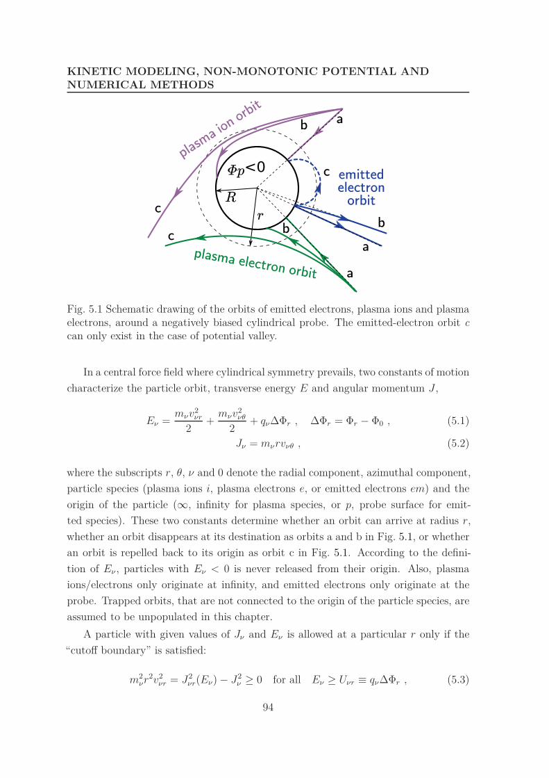
KINETIC MODELING, NON-MONOTONIC POTENTIAL ANDNUMERICAL METHODS
r
a
b
c
a
c
b
plasma io
n orbit
emittedelectron
orbit
Φp<0
R
plasma electron orbit a
bc
Fig. 5.1 Schematic drawing of the orbits of emitted electrons, plasma ions and plasmaelectrons, around a negatively biased cylindrical probe. The emitted-electron orbit ccan only exist in the case of potential valley.
In a central force field where cylindrical symmetry prevails, two constants of motion
characterize the particle orbit, transverse energy E and angular momentum J ,
Eν =mνv2
νr
2+
mνv2νθ
2+ qν∆Φr , ∆Φr = Φr − Φ0 , (5.1)
Jν = mνrvνθ , (5.2)
where the subscripts r, θ, ν and 0 denote the radial component, azimuthal component,
particle species (plasma ions i, plasma electrons e, or emitted electrons em) and the
origin of the particle (∞, infinity for plasma species, or p, probe surface for emit-
ted species). These two constants determine whether an orbit can arrive at radius r,
whether an orbit disappears at its destination as orbits a and b in Fig. 5.1, or whether
an orbit is repelled back to its origin as orbit c in Fig. 5.1. According to the defini-
tion of Eν , particles with Eν < 0 is never released from their origin. Also, plasma
ions/electrons only originate at infinity, and emitted electrons only originate at the
probe. Trapped orbits, that are not connected to the origin of the particle species, are
assumed to be unpopulated in this chapter.
A particle with given values of Jν and Eν is allowed at a particular r only if the
“cutoff boundary” is satisfied:
m2νr2v2
νr = J2νr(Eν) − J2
ν ≥ 0 for all Eν ≥ Uνr ≡ qν∆Φr , (5.3)
94
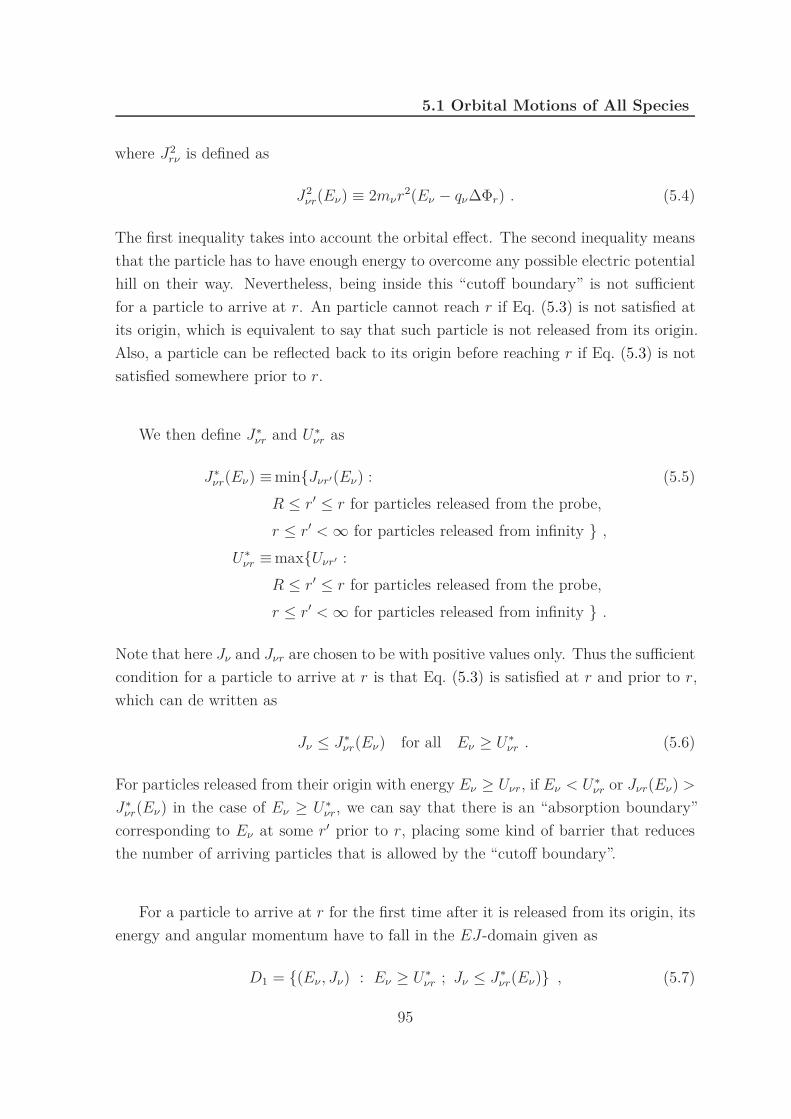
5.1 Orbital Motions of All Species
where J2rν is defined as
J2νr(Eν) ≡ 2mνr2(Eν − qν∆Φr) . (5.4)
The first inequality takes into account the orbital effect. The second inequality means
that the particle has to have enough energy to overcome any possible electric potential
hill on their way. Nevertheless, being inside this “cutoff boundary” is not sufficient
for a particle to arrive at r. An particle cannot reach r if Eq. (5.3) is not satisfied at
its origin, which is equivalent to say that such particle is not released from its origin.
Also, a particle can be reflected back to its origin before reaching r if Eq. (5.3) is not
satisfied somewhere prior to r.
We then define J∗
νr and U∗
νr as
J∗
νr(Eν) ≡ minJνr′(Eν) : (5.5)
R ≤ r′ ≤ r for particles released from the probe,
r ≤ r′ < ∞ for particles released from infinity ,
U∗
νr ≡ maxUνr′ :
R ≤ r′ ≤ r for particles released from the probe,
r ≤ r′ < ∞ for particles released from infinity .
Note that here Jν and Jνr are chosen to be with positive values only. Thus the sufficient
condition for a particle to arrive at r is that Eq. (5.3) is satisfied at r and prior to r,
which can de written as
Jν ≤ J∗
νr(Eν) for all Eν ≥ U∗
νr . (5.6)
For particles released from their origin with energy Eν ≥ Uνr, if Eν < U∗
νr or Jνr(Eν) >
J∗
νr(Eν) in the case of Eν ≥ U∗
νr, we can say that there is an “absorption boundary”
corresponding to Eν at some r′ prior to r, placing some kind of barrier that reduces
the number of arriving particles that is allowed by the “cutoff boundary”.
For a particle to arrive at r for the first time after it is released from its origin, its
energy and angular momentum have to fall in the EJ-domain given as
D1 = (Eν , Jν) : Eν ≥ U∗
νr ; Jν ≤ J∗
νr(Eν) , (5.7)
95

KINETIC MODELING, NON-MONOTONIC POTENTIAL ANDNUMERICAL METHODS
where the subscript 1 denotes the first arrival. For a particle to disappear at its
destination, the EJ-domain is thus
Dd = (Eν , Jν) : Eν ≥ U∗
ν ; Jν ≤ J∗
ν (Eν) , (5.8)
where the subscript d denotes the destination and U∗
ν and J∗(Eν) are defined as
U∗
ν ≡ max qν∆Φr′ ; R ≤ r′ < ∞ , J∗
ν (Eν) ≡ minJνr′(Eν); R ≤ r′ < ∞ . (5.9)
Then for a particle to arrive at the radius r for the second time, as it is reflected back
before arriving at their destination, the EJ-domain is simply
D2 = D1 \ Dd , (5.10)
where the subscript 2 denotes the second arrival.
5.2 Current and Particle Density
5.2.1 Particles from Ambient Plasma at Infinity
Particles coming from plasma have undisturbed Maxwellian distribution at infinity.
Thus the distribution function at r is
f(r, vνr, vνθ) = Nν0mν
2πKTνexp
(− Eν
KTν
). (5.11)
The particle density at r can be found by the integration
Nν(r)
Nν0=∫ ∫
D1+D2
exp(−Eν/KTν) dEν dJν
πKTν
√Jνr
2(E) − J2ν
. (5.12)
The E-integral must be carried out once for vr < 0 (incoming population, or first-
arrival population, as purple/green curves a , b and c in Fig. 5.1) and again for vr > 0
(outgoing population, or second-arrival population, which arrives at r and continues
to move inwards until it turns back outwards at a radius between r and R, without
arriving at the probe, as purple/green curve c). The J-integral has been made to
cover just positive values by writing dJ → 2 dJ . The E-J domain of integration is
determined by the orbital motion theory described in the previous section.
96

5.2 Current and Particle Density
According to Eq. (5.7), the EJ-domain D1 for all orbits that reach r as incoming
orbits are
incoming orbits at r
Eν ≥ U∗
νr ≡ max qνΦr′ ; r ≤ r′ < ∞0 ≤ Jν ≤ J∗
νr(Eν) ≡ minJνr′(Eν); r ≤ r′ < ∞. (5.13)
Similarly, given by Eq. (5.8), the E-J domain Dd for all orbits that reach R without
turning back are
reach the probe
Eν ≥ U∗
ν ≡ max qνΦr′ ; R ≤ r′ < ∞0 ≤ Jν ≤ J∗
ν (Eν) ≡ minJνr′(Eν); R ≤ r′ < ∞. (5.14)
The EJ-domain for outgoing orbits at r can thus be easily acquired by excluding
domain (5.14) from (5.13), D2 = D1 \ Dd. The particle density integration thus
becomes
Nν(r)
Nν0= 2
∫∞
U∗
νr
exp(−Eν/KTν)
πKTνarcsin
J∗
νr(Eν)
Jνr(Eν)dEν
−∫
∞
U∗
ν
exp(−Eν/KTν)
πKTν
arcsinJ∗
ν (Eν)
Jνr(Eν)dEν . (5.15)
The particles that strike on the probe contribute to the final current that is given as
Iν = −2qνNν0Lp
mν
∫∞
U∗
ν
exp(−Eν/KTν)
KTν
J∗
ν (Eν) dEν , (5.16)
where Lp is the probe length and the current is collected if Iν > 0, otherwise emitted.
5.2.2 Particles Emitted by the Probe
Particles emitted by the probe have a half-Maxwellian distribution at probe surface
[115]. Thus the distribution function at r is
f(r, vνr, vνθ) = Nν0mν
πKTνexp
(− Eν
KTν
). (5.17)
The particle density at r can be found by the integration
Nν(r)
Nν0=∫ ∫
D1+D2
2 exp(−Eν/KTν) dEν dJν
πKTν
√Jνr
2(E) − J2ν
. (5.18)
97

KINETIC MODELING, NON-MONOTONIC POTENTIAL ANDNUMERICAL METHODS
The E-integral must be carried out once for outgoing population, as blue curves a , b
and c in Fig. 5.1, and again for incoming population that arrives at r and continues
to move outwards until it turns back inwards at a radius r′ > r, without reaching the
infinity, as blue curve c.
According to Eq. (5.7), the EJ-domain D1 for all orbits that reach r as outgoing
orbits are
outgoing orbits at r
Eν ≥ U∗
νr ≡ max qν (Φr′ − Φp) ; R ≤ r′ < r0 ≤ Jν ≤ J∗
νr(Eν) ≡ minJνr′(Eν); R ≤ r′ < r. (5.19)
Similarly, given by Eq. (5.8), the EJ-domain Dd for all orbits that reach infinity
without turning back are
reach the infinity
Eν ≥ U∗
ν ≡ max qν (Φr′ − Φp) ; R ≤ r′ < ∞0 ≤ Jν ≤ J∗
ν (Eν) ≡ minJνr′(Eν); R ≤ r′ < ∞. (5.20)
The EJ-domain D2 for incoming orbits at r can thus be easily acquired by excluding
domain (5.20) from (5.19). The particle density integration thus becomes
Nν(r)
Nν0
= 4∫
∞
U∗
νr
exp(−Eν/KTν)
πKTν
arcsinJ∗
νr(Eν)
Jνr(Eν)dEν
− 2∫
∞
U∗
ν
exp(−Eν/KTν)
πKTνarcsin
J∗
ν (Eν)
Jνr(Eν)dEν . (5.21)
The particles that successfully reach and disappear at infinity contribute to the final
current that is given as
Iν =4qνNν0Lp
mν
∫∞
U∗
ν
exp(−Eν/KTν)
KTν
J∗
ν (Eν) dEν , (5.22)
where the current is emitted if Iν < 0.
5.3 Normalization
The parameters are all normalized to the quantities of plasma electrons as
ξD ≡ R
λDe, Zν ≡ qν
e, βν ≡ Nν0
Ne∞
, θν ≡ Te
Tν, αν ≡ mν
me. (5.23)
98

5.3 Normalization
The r dependent variables in Poisson’s equation are normalized as:
z ≡ r
R, Ψz ≡ eΦr
KTe, nν ≡ Nν
Nν0, (5.24)
where the subscript 0 denotes the origin of the particles and the particle densities are
normalized to its own density at its origin Nν0 instead of Ne∞. Energies, momenta
and electric potentials are also normalized for each species as
ǫj ≡ Eν
KTν, j2
ν ≡ J2ν
2mνR2KTν, (5.25)
j2νz(ǫν) ≡ J2
νr
2mνR2KTν≡ z2[ǫν − uνz] , (5.26)
uνz ≡ Uνr
KTν≡ Zνθν∆Ψνz ≡ Zνθν (Ψz − Ψν0) , (5.27)
with Ψν0 = Ψp for emitted species and Ψν0 → 0 for plasma species.
Poisson’s equation becomes
1
z
d
dz
(z
dΨ
dz
)= −ξ2
DΣZνβνnν , (5.28)
with the boundary condition being
Ψ = Ψp at z = 1, Ψ → 0 as z → ∞ . (5.29)
The number density of plasma species can be found by integration
nν(z) = 2∫
∞
u∗
νz
exp(−ǫν)
πarcsin
j∗
νz(ǫν)
jνz(ǫν)dǫν
−∫
∞
u∗
ν
exp(−ǫν)
πarcsin
j∗
ν(ǫν)
jνz(ǫν)dǫν ,
(5.30)
where u∗
νz and j∗
νz are defined as
u∗
νz ≡ max ZνθνΨz′; z < z′ < ∞ , j∗
νz(ǫν) ≡ min jνz′(ǫν); z < z′ < ∞ , (5.31)
and u∗
ν and j∗
ν are defined as
u∗
ν ≡ max ZνθνΨz′; 1 < z′ < ∞ , j∗
ν(ǫν) ≡ min jνz′(ǫν); 1 < z′ < ∞ . (5.32)
99
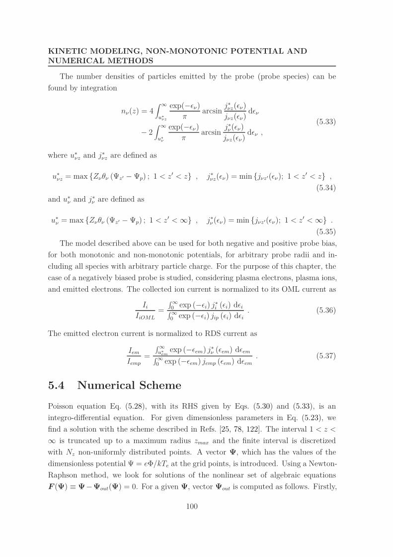
KINETIC MODELING, NON-MONOTONIC POTENTIAL ANDNUMERICAL METHODS
The number densities of particles emitted by the probe (probe species) can be
found by integration
nν(z) = 4∫
∞
u∗
νz
exp(−ǫν)
πarcsin
j∗
νz(ǫν)
jνz(ǫν)dǫν
− 2∫
∞
u∗
ν
exp(−ǫν)
πarcsin
j∗
ν(ǫν)
jνz(ǫν)dǫν ,
(5.33)
where u∗
νz and j∗
νz are defined as
u∗
νz = max Zνθν (Ψz′ − Ψp) ; 1 < z′ < z , j∗
νz(ǫν) = min jνz′(ǫν); 1 < z′ < z ,
(5.34)
and u∗
ν and j∗
ν are defined as
u∗
ν = max Zνθν (Ψz′ − Ψp) ; 1 < z′ < ∞ , j∗
ν(ǫν) = min jνz′(ǫν); 1 < z′ < ∞ .
(5.35)
The model described above can be used for both negative and positive probe bias,
for both monotonic and non-monotonic potentials, for arbitrary probe radii and in-
cluding all species with arbitrary particle charge. For the purpose of this chapter, the
case of a negatively biased probe is studied, considering plasma electrons, plasma ions,
and emitted electrons. The collected ion current is normalized to its OML current as
Ii
IiOML=
∫∞
0 exp (−ǫi) j∗
i (ǫi) dǫi∫∞
0 exp (−ǫi) jip (ǫi) dǫi. (5.36)
The emitted electron current is normalized to RDS current as
Iem
Iemp=
∫∞
u∗
emexp (−ǫem) j∗
ν (ǫem) dǫem∫
∞
0 exp (−ǫem) jemp (ǫem) dǫem. (5.37)
5.4 Numerical Scheme
Poisson equation Eq. (5.28), with its RHS given by Eqs. (5.30) and (5.33), is an
integro-differential equation. For given dimensionless parameters in Eq. (5.23), we
find a solution with the scheme described in Refs. [25, 78, 122]. The interval 1 < z <
∞ is truncated up to a maximum radius zmax and the finite interval is discretized
with Nz non-uniformly distributed points. A vector Ψ, which has the values of the
dimensionless potential Ψ = eΦ/kTe at the grid points, is introduced. Using a Newton-
Raphson method, we look for solutions of the nonlinear set of algebraic equations
F (Ψ) ≡ Ψ−Ψout(Ψ) = 0. For a given Ψ, vector Ψout is computed as follows. Firstly,
100

5.5 Probe Behavior as Emission is Varied
using Ψ, particle densities at the grid points are computed with Eqs. (5.30) and (5.33)
by implementing a Simpson method. Secondly, using a finite-difference method, Ψout
is found by solving Poisson’s Eq. (5.28) with boundary conditions Ψ(1) = Ψp and
Ψ(zmax) ∼ 1/z. The most costly part of the algorithm involves the computation of
the Jacobian of F , which appears in the Newton-Raphson iterative scheme. This
calculation is carried out in parallel by several processors in the code.
In our simulations the values of Nz and zmax were selected as a function of the
parameters Ψp, ξD and β but always within the ranges (256 − 300) and (50 − 150),
respectively. A finer grid was used close to the probe and within the sheath. The
Sympson method in integrals Eqs. (5.30) and (5.33) used 1000 discretization points
and the upper limits were truncated to 7. A solution was taken as valid if the error
1
Nz
Nz∑
i=1
F 2i (5.38)
was below 5 × 10⁻⁸.
Code validation was done in three ways. First it was compared in no-emission con-
ditions with previous Vlasov-Poisson solvers in cylindrical geometry [25, 122]. Second,
once Φ(r) is found, we reconstruct the distribution functions following the procedure
explained in Sec. 5.5.2. We then compare particle densities given by the algorithm
(Eqs. (5.30) and (5.33)) with the ones obtained by integrating the distribution func-
tion in velocity space. At the end, we also compare the Rmax found by this numerical
method to that found by using analytic method in the previous chapter.
5.5 Probe Behavior as Emission is Varied
5.5.1 Currents and Potential Profiles
This section presents some examples of Langmuir probe regimes and plasma structure
as electron emission is varied. Hereafter we fix qi/e = 1 (thus also Ni∞ = Ne∞ = N∞),
qem/e = −1, Ti/Te = 1, and Tp/Te = 0.25. Figure 5.2a shows the normalized ion
and emitted electron densities at the probe, Ni(R)/N∞ and Nem(R)/Nemp, versus the
parameter βem ≡ Nemp/N∞ for eΦp/kTe = −50 and R/λDe = 3. Note that emitted
electron density at the probe Nem(R) is different from the densities of the electrons
that are able to be emitted by the probe to the immediate vicinity of the probe Nemp. If
there is a virtual cathode, some electrons will be reflected back to the probe, leading to
101

KINETIC MODELING, NON-MONOTONIC POTENTIAL ANDNUMERICAL METHODS
0 20 40 60 800
0.5
1
1.5
2
Nemp/N∞
Ni(R)/N∞
Nem(R)/Nemp
Ii/IiOML
Iem/Iemp
(a) Normalized current and density at theprobe for ions and emitted electrons ver-sus the density ratio βem ≡ Nemp/N∞.
0 0.2 0.4 0.6 0.8 10
0.2
0.4
0.6
0.8
1
(R/r)2
Φ/Φp
0 0.02 0.040
0.02
0.04
βem
(b) Normalized potential Φ/Φp versus(R/r)2 for βem = 5 (red dash-dot curve) andβem = 52 (dashed curve). The inset showsthe potential behavior near infinity.
Fig. 5.2 Results from numerical analysis, for parameters values Ti/Te = 1, Tp/Te =0.25, eΦp/kTe = −50 and R/λDe = 3.
Nem(R) > Nemp. The collected ion current Ii normalized with IiOML and the emitted
electron current Iem normalized with Iemp are also shown.
We first note that, for no emission, the selected probe radius R/λDe = 3 is well
above the maximum radius to collect OML ion current, as shown in Fig. 4.6 from the
analytic results. Under these conditions the probe is said to operate beyond OML
regime, i.e., OML forbidden. As a result, for low βem, Ii/IiOML and Ni(R)/N∞ in
Fig. 5.2a are well below 1 and 0.5 that are the values within OML regime. As βem
increases, they approach (but never reach) 1 and 0.5, thus indicating that the probe
operates closer to OML allowed conditions if emission is enhanced. Figure 5.2b shows
a Φ(r)/Φp versus (R/r)2 diagram for βem = 5 and βem = 52. In both cases the
potential profile cuts the diagonal, thus indicating that the probe does not operate
within OML regime (see the inset). Although the ratio r20Φ/R2Φp (see Fig. 4.4), i.e.,
the ordinate-to-abscissa profile ratio of the profile in Fig. 5.2b, increases with βem,
the numerical results suggest that, even in the limit βem → ∞, the probe will never
operate within the OML regime for these parameter values.
For βem . 21.8, all the electrons emitted by the probe are able to reach infinity,
i.e., Iem/Iemp = 1 and Nem(R) = Nemp in Fig. 5.2a and the potential is monotonic.
However, as βem increases, the slope of Φ(r)/Φp in Fig. 5.2b becomes flatter at the
probe. At the critical value β∗
em ∼ 21.8, the electric field at the probe vanishes and the
102

5.5 Probe Behavior as Emission is Varied
0 20 40 60 800
0.5
1
1.5
2
Nemp/N∞
Ni(R)/N∞
Nem(R)/Nemp
Ii/IiOML
Iem/Iemp
(a) Normalized current and density at theprobe for ions and emitted electrons ver-sus the density ratio βem ≡ Nemp/N∞.
0 0.2 0.4 0.6 0.8 10
0.2
0.4
0.6
0.8
1
(R/r)2
Φ/Φp
0 0.005 0.010
0.005
0.01
βem
(b) Normalized potential Φ/Φp versus(R/r)2 for βem = 1 (red dash-dot curve) andβem = 52 (dashed curve). The inset showsthe potential behavior near infinity.
Fig. 5.3 Results from numerical analysis, for parameters values Ti/Te = 1, Tp/Te =0.25, eΦp/kTe = −50 and R/λDe = 1.
current is SCL. For βem > β∗
em the electric field points outwards from the probe and
some electrons come back to the probe because they cannot overcome the potential
hill. Consequently, one has Iem/Iemp < 1 and Nem(R)/Nemp > 1 for βem > β∗
em. As
βem → ∞, Nem(R)/Nemp approaches 2, indicating that most of the electrons are
repelled back to the probe. An example of potential profile within the SCL regime is
given by the blue dashed curve in Fig. 5.2b, which corresponds to βem = 52.
In the previous case the probe did not reach OML conditions but, naturally, this
depends on the specific value of the parameters. For instance, a similar analysis using
R/λDe = 1 instead of R/λDe = 3 gives the results shown in Fig. 5.3. For βem . 2.5,
the probe works beyond the OML regime and beyond SCL regime, shown as the red
dash-dot curve in Fig. 5.2b where the potential profile cuts the diagonal for βem = 1.
For 2.5 . βem . 69.0, the probe works within the OML regime, however beyond the
SCL regime, as the dashed curve in Fig. 5.2b. For βem & 69.0, the probe works within
the OML regime and within the SCL regime.
5.5.2 Density Profiles and Distribution Functions
Figure 5.4 shows the normalized plasma ion, plasma electron and emitted electron
densities for a probe operating with parameters R/λDe = 1 and eΦ0/kTe = −50. Each
panel shows the profiles for βem values equal to 1 (beyond OML and beyond SCL), 50
103

KINETIC MODELING, NON-MONOTONIC POTENTIAL ANDNUMERICAL METHODS
100
101
102
0
0.5
1
a) Ni/N∞
100
101
102
0
0.5
1
b) Ne/N∞
1 1.1 1.2 1.3 1.4 1.5 1.6 1.7 1.8 1.9 20
0.5
1
1.5
2
r/R
c) Nem/Nemp
βem
βem
βem
Fig. 5.4 Normalized density versus radial distance for R/λDe = 1, Ti/Te = 1, Tp/Te =0.25, eΦp/kTe = −50. The βem values are 1, 50 and 90. Panel (a), (b) and (c)correspond to plasma electrons and ions and emitted electrons, respectively. The usedcomputational box was larger than the range shown in the figure. X-axis is in log-scalein panels (b) and (c). In panel (c), x-axis is in linear-scale and only the near-proberegion r ≤ 2R is shown.
(within OML and beyond SCL) and 90 (within OML and within SCL). We remark that
the x-axis is in log-scale in panels (a) and (b) and the computational domains, zmax,
was larger than the radial range shown in Fig. 5.4. Particle emission modifies the radial
structure of the density profiles: both the sheath radius and the maximum reached
by the ion density profile are enhanced as βem increases. For βem = 90, greater than
69 (which is the threshold for SCL condition), the ratio Nem(r)/Nemp reaches values
above 1. In this case, the emitted electron population is composed of both incoming
(vr < 0) and outgoing (vr > 0) electrons for R ≤ r ≤ rm. Here rm corresponds to the
radius where the potential is minimum.
Particle distribution functions can be reconstructed from the potential profile Φ(r).
As we will see, this is an interesting information to understand the behavior of an
104

5.5 Probe Behavior as Emission is Varied
emissive probe and also to check the model given by Eqs. (5.28), (5.30) and (5.33).
For a radius rc, we compute the distribution function of a particle with radial velocity
vrc and azimuthal velocity vθc, i.e., fν(rc, vrc, vθc), as following. According to Newton’s
Second Law mνdv/dt = Fν , there is
dvr
dt= −qν
dΦ
dr+
v2θ
r= −qν
dΦ
dr+
v2θcr
2c
r3, (5.39)
which is integrated backwards in time with the initial condition (vrc, vθc) at rc, until
the trajectory hits the probe or reaches rmax with velocities, say, vrf and vθf . For
plasma species, ν = i, e, the trajectory reaches rmax, we assign to fν the value of a
Maxwellian distribution as in Eq. (5.11), otherwise fν = 0. For emitted electrons,
ν = em, if the trajectory hits the probe, fν is assigned the value of a half Maxwellian
distribution as in Eq. (5.17), otherwise fν = 0. In this way, we can compute the full
distribution function at rc, fν(rc, vrc, vθc), for all velocities.
Here, in particular, we will focus on emitted electrons. And instead of plotting
fν(rc, vrc, vθc) in velocity space, we will use the ǫj-plane, with ǫ the normalized energy
and j the normalized angular momentum, similar to Figs. 2.5 and 4.5.
Figure 5.5 shows the result for parameter values as R/λDe = 1, eΦp/kTe = −50,
and βem = 50. The normalized distribution function, fem(rc, vrc, vθc) ≡ kTpfem/Nempme
is calculated for both zc = rc/R = 1.01 (top panels) and 1.1 (bottom panels), and
for both incoming (left panels) and outgoing population (right panels). The color
of each ǫj-cell represents the normalized distribution function value. As shown in
Fig. 5.3a, the current is not SCL and the potential is monotonic , with zm = 1 and
Φm = Φp. Thus the zm-line j2em = j2
emz(zm, ǫ) (solid green) overlap with the z = 1 line
(dash-dot blue). The zc-line (dashed red) is always to the right of z = 1 line, giving
j∗
emz(z, ǫ) = jemz(1, ǫ) for all z and all ǫ ≥ u∗
emz = 0. Therefore, for both zc = 1.01 and
1.1, all electrons are accelerated outwards without meeting any barrier. As shown in
the left panels, there is no any incoming population. And in the right panels, there is
a population of outgoing electrons covering the range 0 ≤ j ≤ jemz(1, ǫ).
For R/λDe = 1, eΦp/kTe = −50, and βem = 90, the current is SCL according
to Fig. 5.3a. The potential is thus not monotonic anymore, exhibiting a minimum
at zm ≈ 1.043, with the value of potential being Φm/Φp ≈ 1.002. As shown in the
bottom-left panel of Fig. 5.6, for zc = 1.1 > zm, there is no incoming population.
This is because the electrons, that can overcome the potential hill for them in the
region z < zm, would be accelerated all the way beyond zm towards infinity. These
electrons must first have enough energy as ǫ > Zemθem(Ψm − Ψp). In addition, due to
105

KINETIC MODELING, NON-MONOTONIC POTENTIAL ANDNUMERICAL METHODS
Fig. 5.5 Normalized emitted electron distribution function fem(rc, vrc, vθc) ≡kTpf/Nempme in the ǫj-plane for a simulation with R/λDe = 1, eΦp/kTe = −50 andβem = 50. Top and bottom panels correspond to rc/R = 1.01 and rc/R = 1.1 respec-tively. Left and right panels correspond to incoming electrons and outgoing electronsrespectively. The lines j2
em = j2emz(1, ǫ) (dash-dot blue line), j2
em = j2emz(zm, ǫ) (solid
green line), and j2em = j2
emz(zc, ǫ) (dashed red line) are also shown. In the bottompanels, the dashed red line lie far away to the right, outside the frame shown here.
orbit effects, they have to also satisfy the absorption boundary jem ≤ j∗
emz(zm, ǫ) for
these energies. This absorption boundary is given by the dashed curve in Fig. 5.7. The
dashed curve osculates the z = 1 line at some energy value, beyond which they overlap
with each other. In the bottom-right panel of Fig. 5.6, only the low-ǫ range is shown
for this absorption boundary, which is very close to the zm-line. For zc = 1.01 < zm,
shown as the purple lines in Fig 5.7, there are two possibilities. It can osculate the
dashed curve at some point, say, ǫc. For ǫ < ǫc, j∗
emz(zc, ǫ) = jemz(zc, ǫ) while j∗
emz(zc, ǫ)
is given by the dashed curve. Or it can not osculate the dashed curve, only intersects
with the z = 1 line at some point, say, ǫc again. Thus, there are j∗
emz(zc, ǫ) = jemz(zc, ǫ)
for ǫ < ǫc and j∗
emz(zc, ǫ) = jemz(z = 1, ǫ) for ǫ > ǫc. Here we will not go into the details
106

5.5 Probe Behavior as Emission is Varied
Fig. 5.6 Similar to Fig. 5.5 but βem = 90. In this case the potential is not monotonicbut having a minimum at zm ≈ 1.043.
z=zm
j2
z=1
1<zc<zm
Fig. 5.7 Inside the potential hill for emitted electrons, the line for z = 1 and zm
line intersects with each other. And formed by all the z-family lines for 1 ≤ z ≤ zm,the dashed curve marks the absorption boundary for emitted electrons to be able toovercome the potential hill and then move towards infinity. The purple lines representtwo possibilities of zc line for 1 < zc < zm.
107

KINETIC MODELING, NON-MONOTONIC POTENTIAL ANDNUMERICAL METHODS
of these. Just as shown in the top panels, only the low-ǫ range is shown for j∗
emz(zc, ǫ)
and j∗
emz(zm, ǫ), which overlaps with zc-line and zm-line respectively. In the case of
j ≤ j∗
emz(zc, ǫ) for all ǫ > Zemθem(Ψc − Ψp), electrons appear as outgoing population,
as shown in the top-right panel. Bounded by both j∗
emz(zc, ǫ) and j∗
emz(zm, ǫ), there is
the incoming population as shown in the top-left panel.
5.6 Comparison with Analytical Results
To compare with the results from the asymptotic analysis, we reproduce Fig. 4.6 by
calculating the Rmax and dΨ/ dz at the probe for several values of probe bias Ψp using
numeric methods described in this chapter, as markers on the solid curve in Fig. 5.8.
The solid curve is obtained by interpolating these values. The dotted curves with
markers are the results from the asymptotic analysis. The comparison shows good
agreement.
However, as we mentioned before, the point z0 (see Fig. 4.4) is poorly defined in
the asymptotic analysis. Therefore, Rmax is probably not the best subject to compare
because z0 is critical to determine whether the regime is OML or not. However, in
ED tether applications, the Rmax we found is way larger than normal tether radius.
The analytic results, although being lower than that found by numerical methods, still
give a quick and good approximation on OML validity for ED-tether design.
We also compare potential profile calculated for βem = 20, Ψp = −1000 and
R/λDe = 0.912. At this R, the asymptotic analysis shows a profile that lies just on
the diagonal. As shown in Fig. 5.9, the layer-analysis that was used in the analytic
method correctly captures the behavior of the potential at each region.
5.7 Conclusion
From the previous results, we can have several conclusions
• For a negatively biased probe with thermionic electron emission, as the emission
increases, a potential hill for electrons can rise in front of the probe due to space
charge of the emitted electrons, see Fig. 5.2b.
• Same as that found by analytic methods, thermionic emission increases the range
of radius R for OML validity, see Figs. 5.2b and 5.3b.
108

5.7 Conclusion
101
102
103
0.5
1
1.5
2
2.5
3
Ψp
Rmax/λ
D
10 20 30 40 50 60 700
5
10
15
20
25
30
35
Ψp
dΨ/dzatprobe
β = 0
β = 3
β = 20
β = 0 interp
β = 3 interp
β = 20 interp
β = 0 ana
β = 3 ana
β = 20 ana
Fig. 5.8 Comparison between numerical and analytic results on Rmax and the derivativeat the probe for βem = 0, 3 and 20, and for a range of Ψp.
• As shown in Figs. 5.2a and 5.3a, the onset of SCL emission is found as βem ≈ 21.8
for R/λD = 3, while βem ≈ 69.0 for R/λD = 1. Therefore, the larger is the probe
radius, the stronger is the space charge effect.
• Seen from Fig. 5.4, the space charge from emitted electrons enlarges the sheath
radius and increases the amount of ions that enter the sheath
109

KINETIC MODELING, NON-MONOTONIC POTENTIAL ANDNUMERICAL METHODS
10−4
10−3
10−2
10−1
100
10−4
10−3
10−2
10−1
100
(r/R)2
Φ/Φ
p
z0z1ananum
Fig. 5.9 Comparison between numerical can analytic results for the potential profilefor βem = 20, Ψp = −1000 and R/λDe = 0.912.
This numeric analysis provides a consistent model for the probe-plasma interaction,
under conditions of stationary, unmagnetized and isotropic plasmas without trapping.
Not only, this model allows non-monotonic potential to form in front of the probe.
But also, it can be applied for both negative and positive probe, with ion or electron
emission. It can be used to calculate the current profile along a thermionic tether
and implemented in flight simulators to determine the performance of a whole teth-
ered system. Also, this can provide a consistent model for emissive probe operations.
By looking for the floating point, or the inflection point in the constructed I − V
characteristics, the plasma parameters can be derived.
110

Chapter 6
CONCLUSIONS
6.1 Results Review
This thesis proposed a bare thermionic tether which collects and emits current through
its own anodic and cathodic segment respectively, with no recourse to any plasma con-
tactor at tether ends. Anodic electron collection had been proved efficient in the
studies of conventional bare tethers [2, 134]. If the cathodic segment is coated with a
recently developed material, C12A7 : e− electride, which has a possible work function
as low as 0.6 eV and moderately high temperature stability, thermionic emission under
heating in space operation might be well more efficient than “ion collection”. Effi-
cient cathodic contact thus can eliminate the need for an active cathodic end plasma
contactor, such as a hollow cathode, together with its corresponding control/power
subsystems and gas feed. This gives rise to a truly passive propellantless tethered
system for basic tether applications as deorbiting satellites in LEO. In future missions,
with a tether carried on-board, satellites or rocket stages can be dragged down at
the end of their mission and be destroyed in the Earth atmosphere, thus halting the
increase of space debris in LEO and mitigating their threat to other spacecraft and
missions.
To study the operation of bare thermionic tether, it is critical to model the plasma-
tether contact along all the tether length, which is the main goal of this thesis. Each
point on the kilometers-long tether would emit or collect current as if it were part
of a cylindrical probe uniformly polarized at the local tether bias. The disparity
between tether length and tether cross-sectional dimensions allows this 2D simplifi-
cation. Theories on the anodic contact, as current collection around a cylindrical
Langmuir probe, have been well developed [43, 128]. However, this is not the case for
cathodic contact. Involving three charge species, i.e., ambient plasma electrons, ions,
111

CONCLUSIONS
and emitted electrons, two different regimes, i.e., space-charge-limited (SCL) emission
and Richardson-Dushman (RDS) emission, and several transverse layers to couple the
plasma solution and the sheath solution in the asymptotic analysis, this complicated
study is not yet well developed in the theories for emissive probes. This thesis tackled
this problem in three different ways.
First, a preliminary model was proposed for the SCL current around a negatively
biased cylindrical probe which emits electron current. In the 1920s, Langmuir studied
the SCL current between cylindrical electrodes, under assumptions as: vacuum devoid
of ions, cold electrons with zero initial velocities, and zero electric field at the SCL
surface [85]. In this study, we considered the probe as a cathodic electrode emitting
electrons and the plasma sheath edge as an anodic electrode collecting these electrons.
When the current is SCL, the electrons dominate inside the sheath, with ion space
charge being negligible. Emitted electrons have an average kinetic energy as the
temperature of the emitting surface, e.g., Tp ≈ 300 K. They can be considered as cold
electrons with zero initial velocity, compared to the high probe bias |eΦp| ≫ KTp ≈0.03 eV. Along the tether cathodic segment, very near the zero-bias point, although
high-bias assumption is not valid, it does not influence much the total current, similar
to the considerations in the anodic segment near zero-biased point. If the potential
minimum is very close to the probe surface, with a value also close to the probe
potential, the electric field at the probe can thus be considered zero. We then can use
Langmuir’s theory to calculate the SCL current allowed between the cathode probe
and the anode sheath, of which the edge location was obtained using the OML ion
collection [128].
Using this first model, longitudinal current and potential profiles along the SCL
segment were found. Moving towards the cathodic end, increasing the plasma-to-tether
bias, the radial SCL current increases. If it reaches the RDS current at some transition
point B∗, it keeps this constant emission until the cathodic end. Together with the
anodic OML electron collection, we can thus have the current/potential profile, and
then the resultant drag force. Dependent on the ambient parameters, such as plasma
temperature, plasma density, orbital inclination, magnetic field, et cetera, and the
tether geometry, the bare thermionic tether can operate in two different regimes. In
some circumstances, operating in highly inclined orbits or at high altitude, as if the
tether were short, the anodic segment is not able to collect enough electrons and the
current can be emitted fully just by a SCL segment. If more current is collected by
the anodic segment, a SCL segment is followed by a RDS segment, as if the tether
were long. The conditions for the transition of these two operation regimes have been
112

6.1 Results Review
found. In the case of dominant ohmic effect, thermionic emission would result in
a short cathodic segment, or the short circuit current covering most of the cathodic
segment in the case of dominant ohmic effects. Compared to ion collection, thermionic
emission leads to much higher drag values.
This preliminary model, based on Langmuir’s theory, provides a very simple and
fast derivation of the drag production using bare thermionic tethers, which can be im-
plemented into flight simulators to evaluate the tethered system. However, it is still a
crude model and a thorough study of the sheath formation around cylindrical electron-
emitting probes is still necessary. This thesis considered a collisionless, unmagnetized,
and stationary plasma, and solved self-consistently the Poisson-Vlasov system using
both analytical and numerical methods. As Vlasov equation conserves the particle
distribution function along the particle orbits, particle densities can be calculated us-
ing orbital motion theory that is simplified by the cylindrical symmetry. However, the
RHS of Poisson’s equation that is an integro-differential equation, contains not only
the local information at radius r but also elsewhere. Thus the integration can not
be carried out straightforwardly. For this reason, two complementary studies were
carried out (analytical and numerical). They are relevant not only for tethers but also
for emissive Langmuir probes, which are used routinely as the diagnostic device in
laboratory experiments.
Using asymptotic analysis, considering only monotonic radial potential (RDS emis-
sion), high probe bias, and under condition of R = Rmax for OML ion collection,
Poisson’s equation is integrated from infinity towards the probe crossing four different
regions: quasineutral region, two transitional layers to match quasineutrality with the
sheath solution, and the sheath region attached to the probe. At each region, Poisson’s
equation is simplified to include only local information. Layers are smoothly matched
to provide the overall potential structure. It is found that thermionic emission clearly
increases the range of radius R for OML validity. Although emitted electron density
can be negligible faraway in the quasineutral region, its effect can not be generally
neglected throughout the quasineutral region, especially at low bias or with high emis-
sion. At the condition of R = Rmax, the potential bias where the transition from RDS
emission to SCL emission happens is found. This gives a more precise calculation as
compared to Langmuir’s theory. It’s one of the most important results of this thesis.
Using these results, a crude study of the longitudinal tether current/potential pro-
file is also performed considering weak ohmic effects. At a relatively low emission,
SCL-segment length can be short compared to the total tether length, the tether
potential drop along this segment can be small compared to that of the motional
113

CONCLUSIONS
electromotive force, and the current reduction along this segment is also negligible.
Therefore, under weak thermionic/ohmic effects, the necessity for SCL emission mod-
eling can be relieved, together with the complexity of longitudinal analysis. However,
further concrete statement has to be made after the study of the SCL emission is avail-
able. In this case, this asymptotic analysis for the monotonic radial structure that has
been developed in this thesis can be used to model the electron emission beyond the
virtual cathode.
The asymptotic analysis has only been carried out for the condition R = Rmax in
this thesis. Same as imposing the potential of r0 at the diagonal of Fig. 2.6 for this
condition, we can also impose a radius larger than this radius away from this diagonal
and look for the probe radius consistent for this choice. We then can study the probe
response for any radius with R < Rmax, which is the range of interest for thin and light
tethers. For R > Rmax, we can modify the theory presented in Ref. [43] to include
emission. The transition between the RDS and SCL emission can thus be found for
any tether radius. Again, assuming that the potential minimum is close to the probe
in the SCL segment, the emitted current can be approximated by the current that is
allowed to flow with this probe radius, this probe bias and zero electric field at the
probe surface, instead of solving the whole sheath structure as the emitted current is
reduced, being less than the RDS current, by a virtual cathode.
The analytical method developed in this thesis gives physical insight of the problem.
However, as mentioned, it is only under the conditions: R = Rmax, monotonic poten-
tial, and high probe bias. For this reason, the numerical scheme that solve the full
Poisson-Vlasov system, without these assumptions was carried out. It can be applica-
ble for monotonic and non-monotonic radial potential distribution, negative or positive
probe bias, and with ion or electron emission. For solving the time-independent Vlasov
equation, particles densities are formulated using the orbital motion theory and the
integration is carried out by implementing a Simpson method. Poisson’s equation is
then solved using finite difference method. Then a consistent potential profile is found
by using Newton-Raphson iterations to solve the non-linear algebraic equations. It is
again found that thermionic emission increases the R validity for ion OML collection.
It enlarges the sheath radius and attracts more ions into the sheath. Increase of the
probe radius drives the operation regime to be away from within OML regime but
towards within SCL regime. With some large probe radius, it is found that possibly
no any emission level can help the ion collection to be within OML regime. Com-
paring the results from both numerical and analytical methods, about Rmax and the
transition potential for SCL emission to RDS emission at the condition R = Rmax, it
114

6.2 Critical Issues of Bare Thermionic Tethers
shows good agreements. The asymptotic analysis also correctly captured the behavior
of each layer and the matching between them.
Using this numerical scheme, not only can it be used as a basis for the longi-
tudinal analysis of a bare thermionic tether, but also it can be used to predict the
performances of emissive probe by providing current-voltage characteristics. However,
being computationally heavy, Poisson-Vlasov solver can not be directly coupled with
tethered-flight simulators. The parallelized code developed in this thesis could be used
to carry out for massive computations of the emitted current SCL condition, thus giv-
ing the ratio of the actual emitted current to the intrinsic current that depends on the
probe temperature and work function only, as function of a set of parameters:
Iem
Iemp= F
(eΦp
kTe,
Tp
Te,
Ti
Te,
R
λD,
Nemp
Ne,
mi
me
). (6.1)
Although the code is parallelized and fast computation is possible, the parametric
domain is still too broad. First calculation to determine bare thermionic tether perfor-
mance should focus on the particular case, for example, Tp/Te = 0.25 for Tp ≈ 290 K,
Ti = Te, R/λD = 1, Nemp/Ne = 20, and me/mi for oxygen ion. After finding Iem(Φp),
a fitting to this numerical law could be used to determine a more precise current and
potential profile along the tether.
6.2 Critical Issues of Bare Thermionic Tethers
This thesis provides a first study of bare thermionic tethers, of which important re-
search works should be continued in the future, to design a successful mission for
deorbiting satellites using bare thermionic tether, and to make the dream of a clean
and safe space environment come true. This thesis identifies the critical issues of bare
thermionic tethers, which can be organized in two different categories: material issues
and plasma-tether interaction issues.
Material Issues
• As mentioned in the thesis, the emission current is very sensitive to the work
function of the material, see Eq. (3.3). It is critical to find low-work function
materials such as C12A7 : e− electride, and provide a concrete and complete
description about their thermionic characteristics.
115

CONCLUSIONS
• Under real space conditions, ions would strike on the cathodic segment and
change the surface properties of this material. The stability of the material
should be studied in the aspect of sputtering and chemical reaction, which could
modify the thermionic characteristics as we have seen.
• Fabrication of this coating on a kilometers-long tether is not easy. Careless
fabrication process would also modify the thermionic properties.
• The mechanical properties of the coating play a crucial role in reliability of its
functionality. For example, such a coating could experience substantial deforma-
tion during the deployment using a reel or foldaway mechanism.
• The conductivity, thermionic functionality or other properties of this material
could vary under changes of thermal conditions. The response of the material
to the thermal cycle of day-night temperature during tether operations should
be studied.
Plasma-Tether Interaction Issues
• Analytical and numerical methods presented in this thesis can be used to ob-
tain the current-voltage characteristics. This may give more realistic tether
current/voltage profiles as compared to the model based on Langmuir’s theory
in Chap. 3.
• The temperature on the tether is determined by the thermal balance of solar
radiation, ohmic dissipation, heat conduction along the tether, and heat radiated
from the tether. Since the thermionic current depends on the temperature, the
thermal response should be coupled in the current/potential equations along the
tether, as kt in Eq. (3.26) is no longer constant along the tether.
• For conventional bare tethers in LEO, the selection of optimal tether geometry,
considering factors as minimized tether/satellite mass and tether cut probabil-
ity, et cetera, has been recently proposed [135]. For bare thermionic tether,
this should be revised. For example, the sheath formation around an electron-
emitting tape is different from that of a cylinder. The temperature response
under different tether geometry now also plays a crucial part for the emission
since it is directly related to the current exchange efficiency. Such effects should
be included in realistic bare thermionic tether simulators.
116

6.2 Critical Issues of Bare Thermionic Tethers
• We have known that conventional bare tethers are prone to dynamical instabili-
ties [107]. As shown in this thesis, the longitudinal current and voltage profiles
are different between conventional bare tethers and bare thermionic tethers. This
influences the Lorentz torque and the instability analysis should be carried out
again. If such instabilities are found, a passive damper could be used to mitigate
them.
117


References
[1] Ahedo, E., Martinez-Sanchez, M., and Sanmartin, J. Current collectionby an active spherical electrode in an unmagnetized plasma. Physics of FluidsB: Plasma Physics 4 (1992), 3847–3855.
[2] Ahedo, E., and Sanmartin, J. Analysis of bare-tether systems for deorbitinglow-earth-orbit satellites. Journal of Spacecraft and Rockets 39, 2 (2002), 198 –205.
[3] Alfven, H. Spacecraft propulsion: New methods. Science 176, 4031 (1972),167–168.
[4] Alfven, H., and Falthammar, C.-G. Cosmical electrodynamics; fundamen-tal principles. International series of monographs on physics. Oxford, ClarendonPress, 1963.
[5] Allen, J. E., Boyd, R. L. F., and Reynolds, P. The collection of positiveions by a probe immersed in a plasma. Proceedings of the Physical Society.Section B 70, 3 (1957), 297.
[6] Andrienko, A. Y., and Chadaev, A. I. An analysis of capabilities of thegravitational stability augmentation for low orbit satellites. Cosmic Research 36(July 1998), 366.
[7] Artsutanov, Y. Kosmos na elektrovoze (into space by funicular railway).Komsomolskaya Pravda (Young Communist Pravda) (1960).
[8] Aslanov, V., and Ledkov, A. Dynamics of Tethered Satellite Systems.Woodhead Publishing in mechanical engineering. Elsevier Science, 2012.
[9] Beletskii, V., Ivanov, M., and Otstavnov, E. Model problem of a spaceelevator. Cosmic Research 43, 2 (2005), 152 – 156.
[10] Bender, C. M., and Orszag, S. A. Advanced Mathematical Methods forScientists and Engineers I: Asymptotic Methods and Perturbation Theory. NewYork, NY : Springer New York, 1999.
[11] Bernstein, I., and Rabinowitz, I. Theory of electrostatic probes in a lowdensity plasma. Physics of Fluids 2, 2 (1959), 112–121.
119

References
[12] Blash, D. M., and Williams, J. D. Determination of hollow cathode plasmacontactor system requirements using an electrodynamic tether system simulationtool. In 13th Spacecraft Charging and Technology Conference, Pasadena, CA(2014).
[13] Boucher, M. The space elevator: ‘thought experiment’, or key tothe universe? http://spaceref.com/space-elevator/the-space-elevator-thought-experiment-or-key-to-the-universe-by-sir-arthur-c-clarke.html, 2003.
[14] Budden, K. G. Radio waves in the ionosphere; the mathematical theory ofthe reflection of radio waves from stratified ionised layers. Cambridge UniversityPress, 1961.
[15] Carroll, J. A. Tether applications in space transportation. Acta Astronautica13, 4 (1986), 165 – 174.
[16] Chang, K., and Bienkowski, G. Effects of Electron Emission on Electro-static Probes at Arbitrary Pressures. Phys. Fluids 13, 4 (1970), 902.
[17] Charro, M., Sanmartin, J., Bombardelli, C., Sanchez-Torres, A.,Lorenzini, E., Garrett, H., and Evans, R. A proposed two-stage two-tether scientific mission at Jupiter. Plasma Science, IEEE Transactions on 40,2 (Feb 2012), 274–281.
[18] CHEN, F. F. Plasma Diagnostic Techniques. Academic Press, New York, 1965,ch. Electric Probes, pp. 113–200.
[19] Chen, F. F. Introduction to Plasma Physics and Controlled Fusion. Volume 1:Plasma Physics. Boston, MA : Springer US, 1984.
[20] Chen, X., and Sanmartin, J. R. Bare-tether cathodic contact throughthermionic emission by low-work-function materials. Physics of Plasmas (1994-present) 19, 7 (2012), 073508.
[21] Chen, X., and Sanmartin, J. R. Low work-function thermionic emission andorbital-motion-limited ion collection at bare-tether cathodic contact. Physics ofPlasmas 22, 5 (2015), 053504.
[22] Chen, Y., Huang, R., Ren, X., He, L., and He, Y. History of the tetherconcept and tether missions: A review. ISRN Astronomy and Astrophysics 2013(2013). Article ID 502973, 7 pages.
[23] Cherrington, B. The use of electrostatic probes for plasma diagnostics—areview. Plasma Chemistry and Plasma Processing 2, 2 (1982), 113–140.
[24] Child, C. D. Discharge from hot CaO. Physical Review (Series I) 32 (May1911), 492–511.
[25] Choiniere, E. Theory and experimental evaluation of a consistent steady-state kinetic model for 2-D conductive structures in ionospheric plasmas withapplication to bare electrodynamic tethers in space. PhD thesis, University ofMichigan, 2004.
120

References
[26] Chung, P. M., Talbot, L., and Touryan, K. J. Electric probes in station-ary and flowing plasmas: theory and application. Applied physics and engineer-ing: v. 11. New York, Springer-Verlag, 1975.
[27] Chung, S.-J., and Miller, D. W. Propellant-free control of tethered forma-tion flight, part 1: Linear control and experimentation. Journal of Guidance,Control, and Dynamics 31, 3 (May 2008), 571–584.
[28] Chung, S.-J., Slotine, J.-J. E., and Miller, D. W. Propellant-free con-trol of tethered formation flight, part 2: Nonlinear underactuated control. Jour-nal of Guidance, Control, and Dynamics 31, 5 (Sept. 2008), 1437–1446.
[29] Clark, C. C., and Hardy, J. D. Gravity problems in manned space stations.In Proceedings of the Manned Space Stations Symposium, April 20-22, 1960(1960), Institute of the Aeronautical Sciences, pp. 104–113.
[30] Colombo, G., Gaposchkin, E., Grossi, M., and Weiffenbach, G. The«skyhook»: A shuttle-borne tool for low-orbital-altitude research. Meccanica 10,1 (1975), 3–20.
[31] Compton, K. T., and Langmuir, I. Electrical discharges in gases. PartI. Survey of fundamental processes. Reviews of Modern Physics 2 (Apr 1930),123–242.
[32] Cooke, D., and Katz, I. TSS-1R electron currents: magnetic limited collec-tion from a heated presheath. Geophysical Research Letters 25, 5 (1998), 753 –756.
[33] Cosmo, M., and Lorenzini, E. Tethers in space handbook. Tech. rep., NASAMarshall Space Flight Center, 1997. NASA Contract NAG8-1160.
[34] Cramer, D. B. Physiological considerations of artificial gravity. In NASA.Marshall Space Flight Center Applictions of Tethers in Space (1985), vol. 1,p. 13.
[35] Crawford, F. W., and Cannara, A. B. Structure of the double sheath ina hot-cathode plasma. Journal of Applied Physics 36 (1965), 3135 – 3141.
[36] Cronin, J. Modern dispenser cathodes. IEE Proceedings I (Solid-State andElectron Devices) 128 (February 1981), 19–32(13).
[37] Dobrowolny, M., Colombo, G., and Grossi, M. D. Electrodynamics oflong conducting tethers in the near-earth environment. Tech. rep., NASA, 1976.NASA Contract NAS8-31678.
[38] Dobrowolny, M., and Melchioni, E. Electrodynamic aspects of the firsttethered satellite mission. Journal of Geophysical Research: Space Physics 98,A8 (1993), 13761–13778.
[39] Dushman, S. Electron emission from metals as a function of temperature.Physical Review 21 (Jun 1923), 623–636.
121
References
[40] Dye, J. L. Anionic electron in electrides. Nature 365, 6441 (1993), 10.
[41] Edwards, B. C. The space elevator NIAC phase II final report. Tech. rep.,NASA Institute for Advanced Concepts, 2003.
[42] Edwards, B. C., and Westling, E. A. The Space Elevator: A RevolutionaryEarth-to-Space Transportation System. Houston, TX, BC Edward, c2003., 2003.
[43] Estes, R., and Sanmartin, J. Cylindrical langmuir probes beyond theorbital-motion-limited regime. Physics of Plasmas 7, 10 (2000), 4320 – 4325.
[44] Estes, R. D., and Grossi, M. D. Theoretical investigation of EM wave gen-eration and radiation in the ULF, ELF, and VLF bands by the electrodynamicorbiting tether. Tech. rep., Smithsonian Astrophysical Observatory, Cambridge,MA, United States, 1988. NASA Contract Num NAG8-638.
[45] Estes, R. D., Lorenzini, E. C., Sanmartin, J., Pelaez, J., Martinez-Sanchez, M., Johnson, C. L., and Vas, I. E. Bare tethers for electro-dynamic spacecraft propulsion. Journal of Spacecraft and Rockets 37, 2 (Mar.2000), 205–211.
[46] Ferry, J.-B., and Martinez-Sanchez, M. Electron collection by a tetherat high potential in a magnetized plasma. In Joint Propulsion Conferences.American Institute of Aeronautics and Astronautics, July 2003.
[47] Fitzgibbons, T. C., Guthrie, M., Xu, E.-s., Crespi, V. H., David-owski, S. K., Cody, G. D., Alem, N., and Badding, J. V. Benzene-derived carbon nanothreads. Nature Materials 14, 1 (2015), 43 – 47.
[48] Forward, R. Tether transport from LEO to the Lunar surface. In JointPropulsion Conferences. American Institute of Aeronautics and Astronautics,June 1991. AIAA-91-2322.
[49] Forward, R., Hoyt, R., and Uphoff, C. Terminator Tether (TM): Aspacecraft deorbit device. JOURNAL OF SPACECRAFT AND ROCKETS 37,2 (2000), 187 – 196.
[50] Fruchtman, A., Zoler, D., and Makrinich, G. Potential of an emissivecylindrical probe in plasma. Physical Review E 84 (2011), 025402.
[51] Garcia-Pelayo Novo, R. A., Khan, S. B., and Sanmartin, J. R. Sur-vivability analysis of tape-tether against multiple impact with tiny debris. In13th Spacecraft Charging Technology Conference, Pasadena, California, USA,23–27 June 2014 (2014), H. B. Garrett and A. C. Whittlesey, Eds.
[52] Garrick-Bethell, I., and Carr, C. E. Working and walking on smallasteroids with circumferential ropes. Acta Astronautica 61 (Dec. 2007), 1130–1135.
[53] Goebel, D. M., Jameson, K. K., Watkins, R. M., Katz, I., and Mikel-lides, I. G. Hollow cathode theory and experiment. I. Plasma characterizationusing fast miniature scanning probes. Journal of Applied Physics 98, 11 (2005),113302.
122

References
[54] Griffiths, D. J. Introduction to electrodynamics. Boston: Pearson, 2013.
[55] Grossi, M. A ULF dipole antenna on a spaceborne platform of the PPEPLclass. Tech. rep., NASA Marshall Space Flight Cent., 1973. Letter Report onContract NAS8-28303.
[56] Grossi, M. D. Plasma Motor Generator (PMG) electrodynamic tether experi-ment. Tech. rep., Smithsonian Astrophysical Observatory, 1995. NASA ContractNAG9-643.
[57] Gurevich, A. V. Distribution of captured particles in a potential well in theabsence of collisions. Soviet Journal of Experimental and Theoretical Physics 26(Mar. 1968), 575.
[58] Gurnett, D. A., and Bhattacharjee, A. Introduction to plasma physics :with space and laboratory applications. Cambridge, UK ; New York : CambridgeUniversity Press, 2005.
[59] Gyergyek, T., Kovacic1, J., and Cercek, M. Potential formation infront of an electron emitting electrode immersed in a plasma that contains amonoenergetic electron beam. Physics of Plasmas 17 (2010), 083504.
[60] Hastings, D. E., and Wang, J. The radiation impedance of an electrody-namic tether with end connectors. Geophysical Research Letters 14, 5 (1987),519–522.
[61] Hershkowitz, N. How Langmuir probes work. Discharge Parameters andChemistry (1989), 113 – 183.
[62] Hosono, H., Kim, S. W., Miyakawa, M., Matsuishi, S., and Kamiya,T. Thin film and bulk fabrication of room-temperature-stable electrideC12A7 : e− utilizing reduced amorphous 12CaO.7Al2O3(C12A7). Journal ofNon-Crystalline Solids 354, 19–25 (2008), 2772 – 2776.
[63] Hoyt, R., and Minor, B. Remediation of radiation belts using electrostatictether structures. In Aerospace Conference, 2005 IEEE (March 2005), pp. 583–594.
[64] Hull, A. W., and Langmuir, I. Control of an arc discharge by means of agrid. Proceedings of the National Academy of Sciences 15, 3 (1929), 218–225.
[65] Hutchinson, I. H. Principles of plasma diagnostics. Cambridge ; New York :Cambridge University Press, 2002.
[66] Jackson, J. D. Classical electrodynamics. Wiley, 1999.
[67] Jahn, R., and Choueiri, E. Electric propulsion. Encyclopedia of PhysicalScience and Technology 5 (2002), 125 – 141.
[68] Jahn, R. G. Physics of electric propulsion. McGraw-Hill series in missile andspace technology. New York, McGraw-Hill, 1968.
123

References
[69] Janhunen, P. Electric sail for spacecraft propulsion. Journal of Propulsionand Power 20, 4 (July 2004), 763–764.
[70] Janhunen, P. On the feasibility of a negative polarity electric sail. AnnalesGeophysicae 27 (Apr. 2009), 1439–1447.
[71] Janhunen, P., Toivanen, P., Envall, J., Merikallio, S., Montesanti,G., Gonzalez del Amo, J., Kvell, U., Noorma, M., and Lätt, S.Overview of electric solar wind sail applications. Proceedings of the EstonianAcademy of Sciences 63 (2014), 267 – 278.
[72] Katz, I., Gardner, B., Mandell, M., Jongeward, G., Patterson, M.,and Myers, R. Model of plasma contactor performance. Journal of Spacecraftand Rockets 34, 6 (1997), 824 – 828.
[73] Khan, S. B., and Sanmartin, J. R. Analysis of tape tether survival in LEOagainst orbital debris. Advances in Space Research 53, 9 (2014), 1370 – 1376.
[74] Khazanov, G., Stone, N., Krivorutsky, E., Gamayunov, K., andLiemohn, M. Current-induced magnetic field effects on bare tether currentcollection: a parametric study. Journal of Geophysical Research 106, A6 (2001),10565 – 10579.
[75] Kim, S. W., and Hosono, H. Synthesis and properties of 12CaO·7Al2O3electride: review of single crystal and thin film growth. Philosophical Magazine92, 19-21 (2012), 2596–2628.
[76] Laframboise, J. G. Theory of spherical and cylindrical langmuir probes ina collisionless, maxwellian plasma at rest. Tech. rep., University of TorontoInstitute for Aerospace Studies, 1966. UTIAS Report, No. 100.
[77] Laframboise, J. G. Current collection by a positively charged spacecraft: Ef-fects of its magnetic presheath. Journal of Geophysical Research: Space Physics102, A2 (1997), 2417–2432.
[78] Laframboise, J. G., and Parker, L. W. Probe design for orbit-limitedcurrent collection. Physics of Fluids 16, 5 (1973), 629–636.
[79] Lam, S. Unified theory for the Langmuir probe in a collisionless plasma. Physicsof Fluids 8, 1 (1965), 73.
[80] Langmuir, I. The effect of space charge and residual gases on thermioniccurrents in high vacuum. Physical Review 2 (Dec 1913), 450–486.
[81] Langmuir, I. The effect of space charge and initial velocities on the potentialdistribution and thermionic current between parallel plane electrodes. PhysicalReview 21 (Apr 1923), 419–435.
[82] Langmuir, I. Positive ion currents from the positive column of mercury arcs.Science 58, 1502 (1923), 290–291.
124

References
[83] Langmuir, I. Oscillations in ionized gases. Proceedings of the National Academyof Sciences of the United States of America, 8 (1928), 627.
[84] Langmuir, I. The interaction of electron and positive ion space charges incathode sheaths. Physical Review 33 (Jun 1929), 954–989.
[85] Langmuir, I., and Blodgett, K. B. Currents limited by space chargebetween coaxial cylinders. Physical Review 22 (Oct 1923), 347–356.
[86] Langmuir, I., and Blodgett, K. B. Currents limited by space chargebetween concentric spheres. Physical Review 24 (Jul 1924), 49–59.
[87] Langmuir, I., and Compton, K. T. Electrical discharges in gases part ii.fundamental phenomena in electrical discharges. Reviews of Modern Physics 3(Apr 1931), 191–257.
[88] Lindl, J. D. Inertial confinement fusion : the quest for ignition and energygain using indirect drive. AIP Press ; New York, NY, USA : Springer, 1998.
[89] Longuski, J., Tragesser, S., and Puig-Suari, J. Characterization of theoptimal mass problem for aerobraking tethers. Acta Astronautica 44, 5–6 (1999),227 – 241.
[90] Lorenzini, E., and Sanmartin, J. Electrodynamic tethers in space. Scien-tific American 291, 2 (2004), 50 – 57.
[91] Lorenzini, E. C., Cosmo, M. L., Kaiser, M., Bangham, M. E., Von-derwell, D. J., and Johnson, L. Mission analysis of spinning systems fortransfers from low orbits to geostationary. Journal of Spacecraft and Rockets 37,2 (Mar. 2000), 165–172.
[92] Lvov, V., Issacs, J. D., Bradner, H., Backus, G. E., and Vine, A. C.Sky-hook: Old idea. Science 158, 3803 (1967), 946–947.
[93] Marrese-Reading, C., Mackie, B., Polk, J., and Jensen, K. Fieldemission cathodes for electrodynamic tethers: Identifying compatible cathodematerials. AIP Conference Proceedings 608, 1 (2002), 381.
[94] Martinez-Sanchez, M., and Batishchev, O. Advanced electrodynamictether systems: Modeling of scattering and unsteady effects. Tech. rep., AirForce Office of Scientific Research, 2008. AFOSR Grant FA9550-05-1-0380.
[95] Martinez-Sanchez, M., and Hastings, D. E. A systems study of a 100kW electrodynamic tether. The Journal of the Astronautical Science 35 (1987),75–79.
[96] Martinez-Sanchez, M., and Sanmartin, J. R. Artificial auroral effectsfrom a bare conducting tether. Journal of Geophysical Research: Space Physics102, A12 (1997), 27257–27263.
[97] McCurry, J. Scientists in Japan to put Stars-2 satellite into orbitto trial space cleanup. http://www.theguardian.com/science/2014/feb/27/scientists-japan-stars-2-satellite-orbit-space-debris, 2014.
125

References
[98] Mikellides, I. G., Katz, I., Goebel, D. M., and Polk, J. E. Hollowcathode theory and experiment. II. A two-dimensional theoretical model of theemitter region. Journal of Applied Physics 98, 11 (2005), 113303.
[99] Moore, R. The geomagnetic thrustor - a high performance "alfven wave"propulsion system utilizing plasma contacts. In International Electric PropulsionConference (Mar. 1966), American Institute of Aeronautics and Astronautics.AIAA Paper No. 66-257.
[100] Mott-Smith, H. M. History of “Plasmas”. Nature 233 (Sept. 1971), 219.
[101] Mott-Smith, H. M., and Langmuir, I. The theory of collectors in gaseousdischarges. Physical Review 28 (Oct 1926), 727–763.
[102] Nordheim, L. Zur theorie der thermischen emission und der reflexion vonelektronen an metallen. Zeitschrift für Physik 46 (1928), 833–855.
[103] Okawa, Y., Kitamura, S., Kawamoto, S., Iseki, Y., Hashimoto, K.,and Noda, E. An experimental study on carbon nanotube cathodes for elec-trodynamic tether propulsion. Acta Astronautica 61, 11–12 (2007), 989 – 994.
[104] Onishi, T., Martinez-Sanchez, M., Cooke, D. L., and San-martin Losada, J. R. Pic computation of electron current collection to amoving bare tether in the mesothermal condition. In 27th International ElectricPropulsion Conference, 15-19 Oct., Pasadena, California. (2001).
[105] Parks, D. E., and Katz, I. Theory of plasma contactors for electrodynamictethered satellite systems. Journal of Spacecraft and Rockets 24, 3 (May 1987),245–249.
[106] Patterson, M. J., Hamley, J. A., Sarver-Verhey, T. R., and Soulas,G. C. Functional testing of the space station plasma contactor. In 30th JointPropulsion Conference and Exhibit (1994), pp. AIAA PAPER 94–3308.
[107] Pelaez, J., Lorenzini, E. C., Lopez-Rebollal, O., and Ruiz, M. Anew kind of dynamic instability in electrodynamic tethers. Journal of the Astro-nautical Sciences 48, 4 (Oct. 2000), 449–476.
[108] Podgorny, I. M. Topics in Plasma Diagnostics. Boston, MA : Springer US,1971.
[109] Prewett, P. D., and Allen, J. E. The double sheath associated with a hotcathode. Proceedings of the Royal Society A 348 (1976), 435 – 446.
[110] Rand, L., Williams, J., and Hoyt, R. Hollow cathode with electrideinsert. In Joint Propulsion Conferences. American Institute of Aeronautics andAstronautics, July 2011. AIAA 2011-5992.
[111] Rand, L. P. A Calcium Aluminate Electride Hollow Cathode. PhD thesis,Colorado State University, 2014.
126

References
[112] Reimann, A. L. Thermionic emission. London, New York, J. Willey and sons.,1934.
[113] Richardson, O. Some applications of the electron theory of matter. Philo-sophical Magazine Series 6 23, 136 (1912), 594–627.
[114] Richardson, O. The distribution of the molecules of gas in a field of force,with applications to the theory of electrons. Philosophical Magazine Series 6 28,167 (1914), 633–647.
[115] Richardson, O. W. The emission of electricity from hot bodies. Longmans,Green and co., 1916.
[116] Robe, T. R. Stability of two tethered unsymmetrical earth- pointing bodies.AIAA Journal 6, 12 (Dec. 1968), 2282–2288.
[117] Samantha, R., Hastings, D., and Ahedo, E. Systems analysis of electro-dynamic tethers. Journal of Spacecraft and Rockets (1992), 415.
[118] Sanchez-Arriaga, G. A direct Vlasov code to study the non-stationary cur-rent collection by a cylindrical Langmuir probe. Physics of Plasmas 20, 1 (2013),013504.
[119] Sanchez-Arriaga, G., Bombardelli, C., and Chen, X. Impact of non-ideal effects on bare electrodynamic tether performance. Journal of Propulsionand Power 31, 3 (Jan. 2015), 951–955.
[120] Sanchez-Arriaga, G., and Pastor-Moreno, D. Direct Vlasov simulationsof electron-attracting cylindrical Langmuir probes in flowing plasmas. Physicsof Plasmas 21, 7 (2014).
[121] Sanchez-Arriaga, G., and Sanmartin, J. R. Magnetic pumping ofwhistler waves by tether current modulation. Journal of Geophysical Research:Space Physics 115, A2 (2010), n/a–n/a. A02311.
[122] Sanchez-Arriaga, G., and Sanmartín, J. R. Relativistic current collectionby a cylindrical langmuir probe. Physics of Plasmas 19, 6 (2012).
[123] Sanmartin, J., Ahedo, E., and Martinez-Sanchez, M. An anodelesstether generator. In Physics of Charged Bodies in Space Plasmas: Proceedingsof the Workshop Held at Villa Monastero, Varenna, Italy (1991), M. Dobrowolnyand E. Sindoni, Eds., Societa Italiana di Fisica, pp. 201 – 208.
[124] Sanmartin, J., Choiniere, E., Gilchrist, B., Ferry, J.-B., andMartinez-Sanchez, M. Bare-tether sheath and current: Comparison ofasymptotic theory and kinetic simulations in stationary plasma. Plasma Sci-ence, IEEE Transactions on 36, 5 (Oct 2008), 2851–2858.
[125] Sanmartin, J. R. CNES-Space Technology Course: Prevention of Risks Re-lated to Spacecraft Charging. Cepadus, Toulouse, France, 2002, ch. Active charg-ing control and tethers, pp. 515 – 533.
127

References
[126] Sanmartin, J. R. A review of electrodynamic tethers for science applications.Plasma Sources Science and Technology 19, 3 (2010), 034022.
[127] Sanmartin, J. R., Charro, M., Pelaez, J., Tinao, I., Elaskar, S.,Hilgers, A., and Martinez-Sanchez, M. Floating bare tether as upperatmosphere probe. Journal of Geophysical Research: Space Physics 111, A11(2006), A11310.
[128] Sanmartin, J. R., and Estes, R. D. The orbital-motion-limited regime ofcylindrical Langmuir probes. Physics of Plasmas 6, 1 (1999), 395–405.
[129] Sanmartin, J. R., and Estes, R. D. Magnetic self-field effects on currentcollection by an ionospheric bare tether. Journal of Geophysical Research: SpacePhysics 107, A11 (2002), SIA 2–1–SIA 2–7.
[130] Sanmartin, J. R., and Lorenzini, E. C. Exploration of outer planets usingtethers for power and propulsion. Journal of Propulsion and Power 21, 3 (May2005), 573–576.
[131] Sanmartin, J. R., Lorenzini, E. C., and Martinez Sanchez,M. A review of electrodynamic tethers for space applications. In 44thAIAA/ASME/SAE/ASEE Joint Propulsion Conference & Exhibit, Hartford,Connecticut (2009), American Institute for Aeronautics and Astronautics.
[132] Sanmartin, J. R., Lorenzini, E. C., and Martinez-Sanchez, M. Electro-dynamic tether applications and constraints. Journal of Spacecraft and Rockets47, 3 (2010), 442–456.
[133] Sanmartin, J. R., and Martinez-Sanchez, M. The radiation impedanceof orbiting conductors. Journal of Geophysical Research: Space Physics 100, A2(1995), 1677–1686.
[134] Sanmartin, J. R., Martinez-Sanchez, M., and Ahedo, E. Bare wireanodes for electrodynamic tethers. Journal of Propulsion and Power 9, 3 (May1993), 353–360.
[135] Sanmartin, J. R., Sanchez-Torres, A., Khan, S. B., Sanchez-Arriaga, G., and Charro, M. Optimum sizing of bare-tape tethers forde-orbiting satellites at end of mission. submitted to Advances in Space Re-search, 2015.
[136] Sheehan, J. P., and Hershkowitz, N. Emissive probes. Plasma SourcesScience and Technology 20, 6 (2011), 063001.
[137] Sheehan, J. P., Raitses, Y., Hershkowitz, N., Kaganovich, I., andFisch, N. J. A comparison of emissive probe techniques for electric potentialmeasurements in a complex plasma. Physics of Plasmas 18, 7 (2011), 073501.
[138] Singh, D., Krakauer, H., Haas, C., and Pickett, W. Theoretical de-termination that electrons act as anions in the electride Cs+(15−crown−5)2.e−.NATURE 365, 6441 (1993), 39 – 42.
128

References
[139] Sommerfeld, A. Zur elektronentheorie der metalle auf grund der fermischenstatistik. Zeitschrift für Physik 47 (1928), 1–32.
[140] Stone, R. An overview of artificial gravity. Fifth Symposium on the Role ofthe Vestibular Organs in Space Exploration (1973), 23.
[141] Toda, Y., Matsuishi, S., Hayashi, K., Ueda, K., Kamiya, T., Hi-rano, M., and Hosono, H. Field emission of electron anions clathratedin subnanometer-sized cages in [Ca24Al28O64]
4+(4e−). Advanced Materials 16, 8(2004), 685–689.
[142] Toda, Y., Sung Wng, K., Hayashi, K., Hirano, M., Kamiya, T.,Hosono, H., Haraguchi, T., and Yasuda, H. Intense thermal field elec-tron emission from room-temperature stable electride. Applied Physics Letters87, 25 (2005), 254103.
[143] Toda, Y., Yanagi, H., Ikenaga, E., Kim, J., Kobata, M., Ueda, S.,Kamiya, T., Hirano, M., Kobayashi, K., and Hosono, H. Work func-tion of a room-temperature, stable electride [Ca24Al28O64]4+(e−)4. AdvancedMaterials 19, 21 (2007), 3564–3569.
[144] Tonks, L., and Langmuir, I. A general theory of the plasma of an arc. Phys.Rev. 34 (Sep 1929), 876–922.
[145] Tsiolkovsky, K. Dreams of Earth and Sky. The Minerva Group, Inc., 1895.
[146] van Pelt, M. Space Tethers and Space Elevators. Copernicus Books, 2009.
[147] Vannaroni, G., Dobrowolny, M., Lebreton, J., Melchioni, E.,De Venuto, F., Harvey, C., Iess, L., Guidoni, U., Bonifazi, C., andMariani, F. Current-voltage characteristic of the TSS-1R satellite: compari-son with isotropic and anisotropic models. Geophysical Research Letters 25, 5(1998), 749 – 752.
[148] Vontiesenhausen, G. Tethers in space: Birth and growth of a new avenue tospace utilization. Tech. rep., NASA Marshall Space Flight Center, 1984.
[149] Warner, D. J., Branam, R. D., and Hargus, W. A. Ignition and plumecharacteristics of low-current cerium and lanthanum hexaboride hollow cathodes.Journal of Propulsion and Power 26, 1 (Jan. 2010), 130–134.
[150] Wei, R., and Wilbur, P. J. Space-charge-limited current flow in a sphericaldouble sheath. Journal of Applied Physics 60, 7 (1986), 2280–2284.
[151] Wesson, J., and Campbell, D. J. Tokamaks. Oxford science publications.Oxford ; New York : Oxford University Press, 2011.
[152] Wheelock, A., Cooke, D., and Knoll, M. Plasma testing of IProSECcathode devices. In AIAA SPACE 2009 Conferences & Exposition. AmericanInstitute of Aeronautics and Astronautics, Sept. 2009.
129

References
[153] Wilbur, P. J., and Laupa, T. G. Plasma contactor design for electrodynamictether applications. Advances in Space Research 8, 1 (1988), 221 – 224.
[154] Williams, J., Sanmartin, J., and Rand, L. Low work-function coating foran entirely propellantless bare electrodynamic tether. Plasma Science, IEEETransactions on 40, 5 (May 2012), 1441–1445.
[155] Williams, J. D., and Wilbur, P. J. Electron emission from a hollowcathode-based plasma contactor. Journal of Spacecraft and Rockets 29, 6 (1992),820 – 829.
[156] Xie, K., Martinez, R. A., and Williams, J. D. Current–voltage charac-teristics of a cathodic plasma contactor with discharge chamber for applicationin electrodynamic tether propulsion. Journal of Physics D: Applied Physics 47,15 (2014), 155501.
[157] Yoshizumi, T., and Hayashi, K. Thermionic electron emission from a mayen-ite electride–metallic titanium composite cathode. Applied Physics Express 6, 1(2013), 015802.
[158] Zeineh, C. F. Applications of an electrostatic high-voltage tether to radiationbelt remediation. Master’s thesis, Massachusetts Institute of Technology, Dept.of Aeronautics and Astronautics, 2007.
130