universidade federal de santa catarina programa …michael.klug/pesquisa/tese_disse/thesis... ·...
TRANSCRIPT

UNIVERSIDADE FEDERAL DE SANTA CATARINAPROGRAMA DE PÓS-GRADUAÇÃO EM ENGENHARIA
DE AUTOMAÇÃO E SISTEMAS
Michael Klug
CONTROL OF NONLINEAR SYSTEMS USING N-FUZZYMODELS
Florianópolis
2015

Michael Klug
CONTROL OF NONLINEAR SYSTEMS USING N-FUZZYMODELS
A Thesis submitted to the Depar-tament of Automation and SystemsEngineering in partial fulfillmentof the requirements for the degreeof Doctor of Philosophy in Automa-tion and Systems Engineering.Supervisor: Dr. Eugênio de BonaCastelan NetoCo-Supervisor: Dr. Daniel FerreiraCoutinho
Florianópolis
2015
Michael Klug
CONTROL OF NONLINEAR SYSTEMS USING N-FUZZYMODELS
This Thesis is hereby approved and recommended for acceptancein partial fulfillment of the requirement for the degree of “Doctor ofPhilosophy in Automation and Systems Engineering”.
Florianópolis, 7 December 2015.
Dr. Eugênio de Bona Castelan NetoSupervisor
Dr. Daniel Ferreira CoutinhoCo-Supervisor
Dr. Rômulo Silva de OliveiraGraduate Program Coordinator
Examining Comittee:
Dr. Eugênio de Bona Castelan NetoChair
Dr. Reinaldo Martinez Palhares

Dr. Ricardo Coração de Leão Fontoura de Oliveira
Dr. Alexandre Trofino Neto
Dr. Edson Roberto de Pieri
Dr. Hector Bessa Silveira


ABSTRACT
Takagi-Sugeno (T-S) fuzzy models have been extensively investigatedover the last decade to develop the so-called fuzzy model based (FMB)control techniques, providing nonlinear control design methodologieswith a systematic aspect and numerical solution. However, the actualT-S fuzzy modeling techniques, in general, only guarantee the conve-xity of the model and/or their accuracy of representation for a specificdomain of the state space. Thus, for control strategies based on con-vexity properties, the stability of the closed-loop system composed ofthe nonlinear system and the fuzzy controller should be analyzed ina local context, being fundamental to determine stability regions forthe closed-loop system. This inherent local characteristic is often notconsidered in most FMB control design results, which may lead to poorperformance or even instability of the closed-loop system.In this sense, this thesis aims to consider the regional validity of the T-Sfuzzy models for the development of nonlinear discrete-time control sys-tems analysis and design tools, to consider other physical constraintsand to discuss the problems associated with the complexity of T-Sfuzzy models. A modeling method based on the use of nonlinear localrules that provides a compact and accurate representation is presented,allowing also to handle with the dynamic output feedback control pro-blem for systems with nonlinearities that may depend on unmeasurablestates. Using fuzzy Lyapunov functions (FLF), closed-loop stabilityconditions are provided, which can be verified in terms of the feasibilityof a set of linear matrix inequalities (LMIs). The proposed controllersare based on a state and sector nonlinearities feedback, for systemssubject to disturbances bounded in energy or amplitude, and on a dy-namic output feedback, for systems with saturating actuators. Numeri-cal examples are presented throughout this document to illustrate theeffectiveness of the proposed design methodologies. Further, aiming toassist students and engineers in the nonlinear control system design,an interactive computational tool is presented for fuzzy modeling andcontrol. Practical aspects and a study of the digital implementation offuzzy controllers are discussed using a Hardware-in-the-Loop (HIL) si-mulation with a Field Programmable Gate Array (FPGA) developmentboard.
Keywords: nonlinear systems, local stability, T-S fuzzy models, dis-turbances.


RESUMO EXPANDIDO
CONTROLE DE SISTEMAS NÃO LINEARESUTILIZANDO MODELOS N-FUZZY
Palavras-chave: sistemas não lineares, estabilidade local, modelosfuzzy T-S, perturbações.
Introdução
A utilização de modelos fuzzy Takagi-Sugeno (T-S) tem sidoextensivamente investigada no decorrer das últimas décadas, principal-mente por propiciarem o desenvolvimento de metodologias de projetode sistemas de controle não lineares que possuem caráter sistemático esolução numérica. Uma importante razão para isto é que os modelosT-S (TAKAGI; SUGENO, 1985) fornecem uma representação de plantasnão lineares por uma combinação de submodelos lineares locais (ouafins) invariantes no tempo, também chamados de regras, permitindoestender e utilizar de forma natural e elegante alguns resultados e fer-ramentas comuns à teoria de controle robusto e de sistemas linearescom parâmetros variantes (LPV, do inglês Linear Parameter Varying)(MOZELLI; PALHARES, 2011b). Tal combinação de regras é controladapor funções peso-normalizadas, denominadas de funções de pertinên-cia (GAO et al., 2012). Este conceito é mais amplo que a linearizaçãoda planta em um único ponto de interesse, pois possibilita a descriçãoem regiões mais distantes, formando um domínio de operação para osistema.
Muito embora diversos resultados de análise de estabilidade e sín-tese de controladores sejam encontrados na literatura, existem questõescom motivação prática que permanecem em aberto no contexto do con-trole fuzzy baseado em modelo (FMB, do inglês Fuzzy Model Based)(FENG, 2010). Em geral, as técnicas de modelagem fuzzy T-S atu-ais garantem a convexidade do modelo e/ou a sua precisão de repre-sentação somente para uma determinada região do espaço de estados.Desta forma, para estratégias de controle baseadas em propriedadesde convexidade, a estabilidade do sistema de malha fechada formadopelo sistema não linear realimentado pela lei de controle fuzzy deve serestudada no contexto de estabilidade local, sendo fundamental a deter-minação de regiões de estabilidade para o sistema de malha fechada.

Esta importante característica dos modelos fuzzy T-S raramente é con-siderada na literatura, podendo implicar em perda de desempenho e atémesmo instabilidade do sistema em malha fechada (KLUG et al., 2014).Outro problema inerente à utilização de modelos fuzzy T-S diz respeitoao aumento exponencial de complexidade do modelo com o númerode não linearidades presentes no sistema (LAM, 2011), principalmentequando se busca descrever de forma exata a dinâmica do sistema acontrolar, o que implica no aumento da complexidade numérica dosalgoritmos para análise e projeto, assim como do aumento da comple-xidade de implementação de leis de controle.
Neste contexto, esta tese busca evidenciar a importância da con-sideração da validade regional dos modelos fuzzy de tipo T-S para odesenvolvimento de ferramentas de análise e síntese de sistemas de con-trole não lineares, assim como considerar outras restrições físicas pre-sentes no sistema de controle como limites nos atuadores, e discutir aproblemática associada à complexidade dos modelos fuzzy T-S.
Objetivos
De modo geral, um dos problemas que devem ser resolvidos noprojeto de controladores fuzzy T-S aplicados a sistemas não linearesdiz respeito à consideração das restrições impostas tanto pelo processode modelagem, relacionado ao domínio de validade regional do modelo,quanto a restrições físicas comuns aos atuadores, e também na presençade sinais externos comumente encontrados em sistemas reais. Nestecontexto, os seguintes objetivos específicos são estabelecidos:
• Definir um arcabouço de ferramentas teóricas e algorítmicas paraa consideração do domínio de validade dos modelos fuzzy T-Sno projeto de sistemas de controle não lineares, utilizando tam-bém da teoria de estabilidade de Lyapunov para a construção deconjuntos contrativos de forma a estimar a região de atração dosistema de malha fechada (calcular regiões de estabilidade);
• Formalizar um processo de modelagem com redução do númerode regras que possibilite uma menor complexidade numérica, per-mitindo também a implementação de controladores por realimen-tação dinâmica de saídas com não linearidades que dependam deestados não mensuráveis do sistema. Este processo de modelagemé baseado na utilização de modelos fuzzy T-S com submodelos nãolineares locais, denominados neste trabalho de modelos N-fuzzy;
• Desenvolver condições de análise de estabilidade e síntese de con-troladores com garantia de desempenho para sistemas não lineares
representados por modelos N-fuzzy, levando em consideração odomínio de validade regional com estimação de regiões de estabi-lidade e perturbações externas, como as de energia limitada e/ouas de amplitude limitada;
• Efetuar simulações Hardware-in-the-Loop (HIL) considerando queas plantas sejam emuladas virtualmente e os controladores imple-mentados em uma plataforma programável real, a fim de analisara complexidade de implementação digital de controladores fuzzyclássicos e N-fuzzy;
• Prover uma ferramenta interativa à comunidade científica rela-cionada com vistas a auxiliar estes usuáros no projeto de controlenão linear usando técnicas fuzzy.
Contextualização
A lógica fuzzy foi introduzida pelo professor Lofti A. Zadeh daUniversidade da Califórnia, a qual definiu uma nova teoria de conjuntos(ZADEH, 1965). O princípio fundamental desta lógica é que um determi-nado elemento pode pertencer, em um certo grau, a um conjunto e, emum outro grau, a um outro conjunto. Nota-se este tipo de relação depertinência em várias situações da natureza e na vida cotidiana. Estapercepção foi relacionada posteriormente à similaridade com o com-portamento humano na solução de problemas complexos, permitindopor exemplo, que o projetista utilize o conhecimento experimental paraelaborar o projeto de controle do seu sistema. Desde então, a teoria delógica fuzzy tem sido utilizada com sucesso em diversas aplicações deengenharia, e dentre as várias arquiteturas existentes, destaca-se o usodos modelos fuzzy T-S (FENG, 2010).
Os modelos fuzzy T-S baseiam-se na utilização de um conjuntode regras fuzzy para descrever um sistema não linear em termos de sub-modelos lineares/afins invariantes no tempo e locais, conectados porfunções de pertinência que controlam a lei de interpolação entre as re-gras. Esta representação facilita, através da utilização da teoria de Lya-punov, a descrição dos problemas de controle na forma de desigualdadesmatriciais lineares (LMIs, do inglês Linear Matrix Inequalities) (BOYD
et al., 1994), e portanto a obtenção de solução numérica confiável. Ummétodo comum é o uso de funções de Lyapunov quadráticas, ao qualporém, em geral, conduzem a resultados conservadores. Recentemente,funções de Lyapunov fuzzy (FLF, do inglês Fuzzy Lyapunov Function)tem sido utilizadas para se obter condições de projeto menos conser-
vadores ao custo de um aumento da carga computacional (GUERRA;
VERMEIREN, 2004).Neste contexto, o número de regras para representação do mo-
delo T-S pode tornar o problema de projeto de controle computacional-mente intratável, ao qual poucos estudos se destinam a reduzir o númerode regras mantendo a descrição exata do sistema original. Excetuam-seos trabalhos de Dong, Wang & Yang (2009, 2010) e Klug & Castelan(2011), ao qual admitem que determinados termos não lineares per-tencentes a setores limitados apareçam explicitamente nos submodeloslocais. Isto é perfeitamente aplicável na prática, visto que uma grandeclasse de não linearidades verificam condições de setor ao menos lo-calmente, além de trazer o mecanismo matemático desenvolvido paralidar com não linearidades de setor para o controle de sistemas FMB(LIBERZON, 2006).
Outros aspectos práticos estão relacionados com não linearidadesinerentes aos atuadores, tais como saturação, zona morta e/ou histerese.Por exemplo, a presença de saturação (TARBOURIECH et al., 2011a)pode causar efeitos indesejados, como o surgimento de ciclos limitese pontos de equilíbrio, deterioração do desempenho e até mesmo ins-tabilidade do sistema de malha fechada. Além disso, a importantecaracterística de validade local de convexidade dos modelos fuzzy T-Snormalmente não é considerada na literatura, podendo comprometero uso dos controladores obtidos por estas metodologias, com a possi-bilidade do sistema de controle violar os limites seguros de operação,perder desempenho ou até mesmo instabilizar as trajetórias do sistemade malha fechada.
Contribuições da Tese
Dentre as contribuições da pesquisa realizada, no Capítulo 2 éapresentado a formalização de uma técnica de modelagem fuzzy baseadana utilização de submodelos não lineares que permite a redução donúmero de regras fuzzy sem comprometer a exatidão da representação.Esta metodologia pode ser uma importante fonte de redução de com-plexidade numérica, facilitando a obtenção de soluções factíveis ao pro-blema de controle posteriormente definido. Além disso, a flebilidadeproporcionada por esta metodologia permite ao projetista modificar alei de controle convenientemente, para possuir ou não termos de reali-mentação do vetor de não linearidades de setor, tornando possível porexemplo a implementação de controladores por realimentação dinâmicade saídas de sistemas que possuam não linearidades que dependam de

estados não mensuráveis do sistema. Nos Capítulos 3, 4 e 5, partindoda utilização de funções de Lyapunov fuzzy para definir condições deestabilidade para o sistema em malha fechada, obtém-se ferramentaisbaseados em desigualdades matriciais lineares, aos quais são utiliza-dos para o projeto de controladores. Os controladores propostos sãobaseados na realimentação de estados e do vetor de não linearidadesde setor, ao qual são consideradas perturbações limitadas em energiaou amplitude, e na realimentação dinâmica de saídas, para sistemasnão perturbados com atuadores saturantes ou para sistemas sujeitos aperturbações persistentes. Em todos os casos a importante caracterís-tica local da modelagem fuzzy T-S é levada em consideração na fase deprojeto, ao qual através de uma condição de inclusão garante-se que astrajetórias do sistema de malha fechada evoluam apenas no interior dodomínio garantido de validade de convexidade do modelo fuzzy T-S.
Além disso, objetivando auxiliar estudantes, engenheiros e pes-quisadores na análise e projeto de controle de sistemas não lineares,apresenta-se no Capítulo 6 o desenvolvimento de uma ferramenta com-putacional interativa para a modelagem e controle fuzzy. Complemen-tarmente, aspectos práticos e um estudo da complexidade de imple-mentação digital de controladores fuzzy são discutidos através de umasimulação Hardware-in-the-Loop (HIL) com utilização de uma placa dedesenvolvimento FPGA (do inglês Field Programmable Gate Array).
Conclusão
Nesta tese, novas abordagens para o projeto de controladoresaplicados a sistemas não lineares em tempo discreto que possam ser re-presentados por modelos fuzzy T-S são desenvolvidas. Considera-se ummétodo alternativo de modelagem baseado no uso de regras não lineareslocais, que possibilita os seguintes benefícios: i) redução do número deregras em relação a abordagem clássica, que conduz a uma diminuiçãoda complexidade numérica mantendo a exatidão da representação e ii)flexibilidade no controle, permitindo o projeto e implementação práticade controladores por realimentação dinâmica de saídas na presença denão linearidades que dependam de estados não mensuráveis do sistema.Além disso, os resultados propostos consideram os problemas inerentesao projeto de controle, tais como a validade regional dos modelos fuzzyT-S, restrições físicas nos atuadores, e a presença de sinais externosusualmente encontrados em sistemas reais. Exemplos numéricos sãoapresentados ao longo do trabalho com o objetivo de ilustrar a eficiên-cia dos métodos propostos.


LIST OF FIGURES
1 T-S fuzzy models for nonlinear systems . . . . . . . . . 272 Sector nonlinearities . . . . . . . . . . . . . . . . . . . . 313 Typical nonlinearities . . . . . . . . . . . . . . . . . . . 334 Membership functions h(i)(k) for N-fuzzy model . . . . . 465 Membership functions h(i)(k) for classical model . . . . 476 Comparison of the number of rules . . . . . . . . . . . . 487 Membership functions (MFs): α1(x) and α2(x) . . . . . 508 Nonlinear function . . . . . . . . . . . . . . . . . . . . . 519 T-S fuzzy representation . . . . . . . . . . . . . . . . . . 5110 Modeling error when MFs are clipped for x(k) /∈ X . . . 5111 Nonlinear membership functions h(i)(k), ∀ i = 1, ..., 4 . . 5212 Regions and trajectories for motivating example . . . . . 5313 Nonlinear membership functions h(i)(k), ∀ i = 1, ..., 2 . . 6914 Basin of attraction and S0 . . . . . . . . . . . . . . . . . 7015 State trajectories and control effort . . . . . . . . . . . . 7016 Basin of attraction and associated sets . . . . . . . . . . 7217 State trajectories for example 1 . . . . . . . . . . . . . . 7218 Lyapunov Functions: “” for λ = 1 and “×” for λ = 0.9 7319 Domain of validity, trajectories, and ℓ2-gain . . . . . . . 8620 Regions and trajectories for the optimization algorithms 8821 Regions and trajectories . . . . . . . . . . . . . . . . . . 8922 Control effort . . . . . . . . . . . . . . . . . . . . . . . . 8923 Stability characterization for a persistent disturbance
and a nonzero initial condition (IC). . . . . . . . . . . . 9324 Disturbance signal for numerical example . . . . . . . . 11125 Ellipsoidal sets and trajectories for example i) . . . . . . 11226 Ellipsoidal sets and trajectories for example ii) . . . . . 11327 State trajectories for example ii) . . . . . . . . . . . . . 11328 Ellipsoidal sets and trajectories for example iii) . . . . . 11429 State trajectories for example iii) . . . . . . . . . . . . . 11530 Number of downloads . . . . . . . . . . . . . . . . . . . 11831 Initial window . . . . . . . . . . . . . . . . . . . . . . . . 11932 Approximate modeling module window . . . . . . . . . . 12033 Exact modeling module window . . . . . . . . . . . . . . 12234 Control design program window . . . . . . . . . . . . . . 12535 FPGA development board DE2 − 115 . . . . . . . . . . 12736 FPGA prototyping workflow . . . . . . . . . . . . . . . . 127

37 FPGA-in-the-loop structure . . . . . . . . . . . . . . . . 12838 State trajectory x(k) . . . . . . . . . . . . . . . . . . . . 13539 Quantization error . . . . . . . . . . . . . . . . . . . . . 13540 Typical membership functions . . . . . . . . . . . . . . . 15441 Operation points . . . . . . . . . . . . . . . . . . . . . . 15542 Global sector for ϕ = 3
10 x(2)(1 + sin(x(2))) . . . . . . . 16043 Mesh transformation . . . . . . . . . . . . . . . . . . . . 17044 Comparison of numerical complexity . . . . . . . . . . . 17645 Projection of an ellipse . . . . . . . . . . . . . . . . . . . 18246 Projection of an ellipsoid . . . . . . . . . . . . . . . . . . 183

LIST OF TABLES
1 Disturbance tolerance . . . . . . . . . . . . . . . . . . . 872 Disturbance attenuation . . . . . . . . . . . . . . . . . . 873 Number of operations . . . . . . . . . . . . . . . . . . . 1334 Compilation time (in minutes) . . . . . . . . . . . . . . 1345 Hardware occupation . . . . . . . . . . . . . . . . . . . . 1346 Numerical complexity parameters for Case 1 . . . . . . . 1767 Numerical complexity parameters for Case 2 . . . . . . . 176


ABBREVIATIONS
FMB Fuzzy Model Based . . . . . . . . . . . . . . . . . . . . . . . . . . . . . . . . . . . . . 27
T-S Takagi-Sugeno . . . . . . . . . . . . . . . . . . . . . . . . . . . . . . . . . . . . . . . . . . 27
LMI Linear Matrix Inequalities . . . . . . . . . . . . . . . . . . . . . . . . . . . . . . . 27
LPV Linear Parameter Varying . . . . . . . . . . . . . . . . . . . . . . . . . . . . . . . 30
FLF Fuzzy Lyapunov Functions . . . . . . . . . . . . . . . . . . . . . . . . . . . . . . 30
PDC Parallel Distributed Compensation . . . . . . . . . . . . . . . . . . . . . . 30
ISS Input-to-State Stability . . . . . . . . . . . . . . . . . . . . . . . . . . . . . . . . . 34
UB Ultimate Bounded . . . . . . . . . . . . . . . . . . . . . . . . . . . . . . . . . . . . . . 34
HIL Hardware-in-the-Loop . . . . . . . . . . . . . . . . . . . . . . . . . . . . . . . . . . . 35
FPGA Field Programmable Gate Array . . . . . . . . . . . . . . . . . . . . . . . . 36
NPV Nonlinear Parameter Varying . . . . . . . . . . . . . . . . . . . . . . . . . . . 39
SNA Sector Nonlinearity Approach . . . . . . . . . . . . . . . . . . . . . . . . . . . 41
MF Membership Function . . . . . . . . . . . . . . . . . . . . . . . . . . . . . . . . . . . 50
LA Local Asymptotic . . . . . . . . . . . . . . . . . . . . . . . . . . . . . . . . . . . . . . . 62
ℓ2-ISS Input-to-State Stability in the ℓ2-sense . . . . . . . . . . . . . . . . . . 75
OP Operation Point . . . . . . . . . . . . . . . . . . . . . . . . . . . . . . . . . . . . . . . . . 120
LTI Linear-Time Invariant . . . . . . . . . . . . . . . . . . . . . . . . . . . . . . . . . . . 124
GPP General Purpose Processor . . . . . . . . . . . . . . . . . . . . . . . . . . . . . . 126
ASIC Application Specific Integrated Circuit . . . . . . . . . . . . . . . . . . 126
HDL Hardware Description Language . . . . . . . . . . . . . . . . . . . . . . . . . 126
FFT Fast Fourier Transform. . . . . . . . . . . . . . . . . . . . . . . . . . . . . . . . . . 129
LUT Look-Up Table . . . . . . . . . . . . . . . . . . . . . . . . . . . . . . . . . . . . . . . . . . 129
MCR Matlab Compiler Runtime. . . . . . . . . . . . . . . . . . . . . . . . . . . . . . . 136
FLOP Floating Point Operations . . . . . . . . . . . . . . . . . . . . . . . . . . . . . . . 173

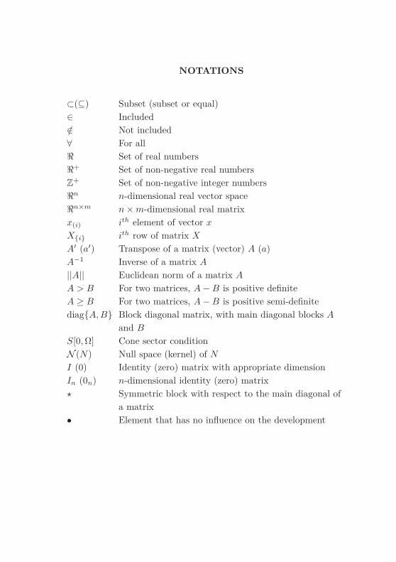
NOTATIONS
⊂(⊆) Subset (subset or equal)
∈ Included
/∈ Not included
∀ For all
ℜ Set of real numbers
ℜ+ Set of non-negative real numbers
Z+ Set of non-negative integer numbers
ℜn n-dimensional real vector space
ℜn×m n × m-dimensional real matrix
x(i) ith element of vector x
Xi ith row of matrix X
A′ (a′) Transpose of a matrix (vector) A (a)
A−1 Inverse of a matrix A
||A|| Euclidean norm of a matrix A
A > B For two matrices, A − B is positive definite
A ≥ B For two matrices, A − B is positive semi-definite
diagA, B Block diagonal matrix, with main diagonal blocks A
and B
S[0, Ω] Cone sector condition
N (N) Null space (kernel) of N
I (0) Identity (zero) matrix with appropriate dimension
In (0n) n-dimensional identity (zero) matrix
⋆ Symmetric block with respect to the main diagonal of
a matrix
• Element that has no influence on the development

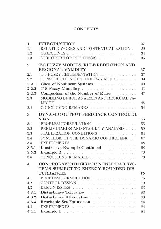
CONTENTS
1 INTRODUCTION 271.1 RELATED WORKS AND CONTEXTUALIZATION . . 291.2 OBJECTIVES . . . . . . . . . . . . . . . . . . . . . . . . 341.3 STRUCTURE OF THE THESIS . . . . . . . . . . . . . 35
2 T-S FUZZY MODELS, RULE REDUCTION ANDREGIONAL VALIDITY 37
2.1 T-S FUZZY REPRESENTATION . . . . . . . . . . . . . 372.2 CONSTRUCTION OF THE FUZZY MODEL . . . . . . 392.2.1 Class of Nonlinear Systems . . . . . . . . . . . . . . 402.2.2 T-S Fuzzy Modeling . . . . . . . . . . . . . . . . . . . 412.2.3 Comparison of the Number of Rules . . . . . . . . 472.3 MODELING ERROR ANALYSIS AND REGIONAL VA-
LIDITY . . . . . . . . . . . . . . . . . . . . . . . . . . . 482.4 CONCLUDING REMARKS . . . . . . . . . . . . . . . . 54
3 DYNAMIC OUTPUT FEEDBACK CONTROL DE-SIGN 55
3.1 PROBLEM FORMULATION . . . . . . . . . . . . . . . 553.2 PRELIMINARIES AND STABILITY ANALYSIS . . . . 593.3 STABILIZATION CONDITIONS . . . . . . . . . . . . . 643.4 SYNTHESIS OF THE DYNAMIC CONTROLLER . . . 673.5 EXPERIMENTS . . . . . . . . . . . . . . . . . . . . . . 683.5.1 Illustrative Example Continued . . . . . . . . . . . . 683.5.2 Example 2 . . . . . . . . . . . . . . . . . . . . . . . . . 703.6 CONCLUDING REMARKS . . . . . . . . . . . . . . . . 73
4 CONTROL SYNTHESIS FOR NONLINEAR SYS-TEMS SUBJECT TO ENERGY BOUNDED DIS-TURBANCES 75
4.1 PROBLEM FORMULATION . . . . . . . . . . . . . . . 754.2 CONTROL DESIGN . . . . . . . . . . . . . . . . . . . . 794.3 DESIGN ISSUES . . . . . . . . . . . . . . . . . . . . . . 834.3.1 Disturbance Tolerance . . . . . . . . . . . . . . . . . 834.3.2 Disturbance Attenuation . . . . . . . . . . . . . . . . 834.3.3 Reachable Set Estimation . . . . . . . . . . . . . . . 844.4 EXPERIMENTS . . . . . . . . . . . . . . . . . . . . . . 844.4.1 Example 1 . . . . . . . . . . . . . . . . . . . . . . . . . 84

4.4.2 Example 2 . . . . . . . . . . . . . . . . . . . . . . . . . 864.5 CONCLUDING REMARKS . . . . . . . . . . . . . . . . 89
5 CONTROL SYNTHESIS FOR NONLINEAR SYS-TEMS SUBJECT TO AMPLITUDE BOUNDEDDISTURBANCES 91
5.1 PROBLEM FORMULATION . . . . . . . . . . . . . . . 915.1.1 Nonlinear State Feedback Design . . . . . . . . . . . 945.1.2 Dynamic Output Feedback . . . . . . . . . . . . . . . 955.2 CONTROL DESIGN . . . . . . . . . . . . . . . . . . . . 975.2.1 State Feedback Design . . . . . . . . . . . . . . . . . 975.2.2 Dynamic Output Feedback . . . . . . . . . . . . . . . 1035.3 DESIGN ISSUES . . . . . . . . . . . . . . . . . . . . . . 1075.3.1 State and Sector Nonlinearities Feedback Design 1075.3.1.1 Minimization of EI . . . . . . . . . . . . . . . . . . . . . 1075.3.1.2 Maximization of EE . . . . . . . . . . . . . . . . . . . . . 1075.3.1.3 Multiobjective Problem . . . . . . . . . . . . . . . . . . . 1085.3.2 Dynamic Output Feedback Design . . . . . . . . . . 109
5.3.2.1 Minimization of EaI . . . . . . . . . . . . . . . . . . . . 109
5.3.2.2 Maximization of EaE . . . . . . . . . . . . . . . . . . . . 109
5.3.2.3 Multiobjetive Problem . . . . . . . . . . . . . . . . . . . 1105.4 EXPERIMENTS . . . . . . . . . . . . . . . . . . . . . . 1105.5 CONCLUDING REMARKS . . . . . . . . . . . . . . . . 115
6 INTERACTIVE SOFTWARE AND HARDWAREIMPLEMENTATION 117
6.1 INTERACTIVE SOFTWARE FOR MODELING ANDCONTROL DESIGN . . . . . . . . . . . . . . . . . . . . 117
6.1.1 Modeling Application . . . . . . . . . . . . . . . . . . 1196.1.1.1 Approximate Modeling Module . . . . . . . . . . . . . . 1206.1.1.2 Exact Modeling Module . . . . . . . . . . . . . . . . . . 1226.1.2 Control Application . . . . . . . . . . . . . . . . . . . 1236.2 HIL IMPLEMENTATION . . . . . . . . . . . . . . . . . 1266.2.1 FPGA-in-the-loop Structure . . . . . . . . . . . . . . 1286.2.2 Requirements and Development Stages . . . . . . . 1296.2.3 Complexity of Implementation . . . . . . . . . . . . 1306.2.3.1 Nonlinear System . . . . . . . . . . . . . . . . . . . . . . 1316.2.3.2 Results . . . . . . . . . . . . . . . . . . . . . . . . . . . . 1326.3 CONCLUDING REMARKS . . . . . . . . . . . . . . . . 135
7 CONCLUSION 1377.1 CONTRIBUTIONS OF THE THESIS . . . . . . . . . . 138
7.2 PERSPECTIVES . . . . . . . . . . . . . . . . . . . . . . 140
References 141
APPENDIX A -- Approximate Modeling 153
APPENDIX B -- Examples of Fuzzy Models 159
APPENDIX C -- Mesh Transformation 169
APPENDIX D -- Conditions of Literature and NumericalComplexity Analysis 173
APPENDIX E -- Projections 181

1 INTRODUCTION
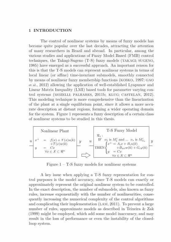
The control of nonlinear systems by means of fuzzy models hasbecome quite popular over the last decades, attracting the attentionof many researchers in Brazil and abroad. In particular, among thevarious studies and applications of Fuzzy Model Based (FMB) controltechniques, the Takagi-Sugeno (T-S) fuzzy models (TAKAGI; SUGENO,1985) have emerged as a successful approach. An important reason forthis is that the T-S models can represent nonlinear systems in terms oflocal linear (or affine) time-invariant submodels, smoothly connectedby means of nonlinear fuzzy membership functions (KOSKO, 1997; GAO
et al., 2012) allowing the application of well-established Lyapunov andLinear Matrix Inequality (LMI) based tools for parameter varying con-trol systems (MOZELLI; PALHARES, 2011b; KLUG; CASTELAN, 2012).This modeling technique is more comprehensive than the linearizationof the plant at a single equilibrium point, since it allows a more accu-rate description at distant regions, forming a wider operating domainfor the system. Figure 1 represents a fuzzy description of a certain classof nonlinear systems to be studied in this thesis.
uu yy
Nonlinear Plant T-S Fuzzy Model
x+ = f(x) + V (x)u(k)+T (x)w(k)
y = Cx∀x ∈ X ⊂ ℜn
Ri :IF ν1 is M i
1 and ... νs is M ins
THEN
x+ = Aix + Biu(k)+Bwiw(k) + Giϕ(k)
y = Cx
∀x ∈ X ⊂ ℜn
Figure 1 – T-S fuzzy models for nonlinear systems
A key issue when applying a T-S fuzzy representation for con-trol purposes is the model accuracy, since T-S models can exactly orapproximately represent the original nonlinear system to be controlled.In the exact description, the number of submodels, also known as fuzzyrules, increase exponentially with the number of nonlinearities, conse-quently increasing the numerical complexity of the control algorithmsand complicating their implementation (LAM, 2011). To prevent a largenumber of rules, approximate models as described in Teixeira & Zak(1999) might be employed, which add some model inaccuracy, and mayresult in the loss of performance or even the instability of the closed-loop system.

28
Even though the exact T-S fuzzy representation has identical dy-namics1 to the original nonlinear system, the convexity of the modelcan only be guaranteed in a specific domain of the state space. Thus,for control strategies based on convex properties, the performance anddynamic behavior of the control system composed of the feedback in-terconnection of the nonlinear plant and the fuzzy controller may dete-riorate if the system states evolve outside this domain. This inherentlocal characteristic of the fuzzy model should be taken into accountwhen using fuzzy controllers applied to nonlinear plants, whether inthe design phase, as considered in this work, or in subsequent analy-sis. This important aspect, which directly affects the practical results,is rarely considered in literature, and imposes the use of local stabi-lity concepts that, in consequence, can be dealt with the definition ofcontractive sets. The notion of contractive sets is basic to determineasymptotic stability regions for nonlinear systems, usually performedusing Lyapunov functions. In this way, regions of admissible initial con-ditions that asymptotically converge to the origin are found (OLIVEIRA
et al., 2011), and can be used as estimates of the domain of attractionof the closed-loop system (KHALIL, 2003).
In recent works, such as the articles Chadli & Guerra (2012), Liet al. (2014) and Zhu et al. (2015), a numerical complexity reduction ofthe control algorithms is obtained by decreasing the number of LMIs tobe solved using the representation of nonlinear plants by descriptor sys-tems. However, this approach does not effectively reduce the numberof rules in the T-S fuzzy model, and few studies commit to maintainingthe exact description of the original system. Some exceptions are theworks Dong, Wang & Yang (2009, 2010), nevertheless without consi-dering the T-S fuzzy models local characteristic, and the works Klug& Castelan (2011) and Klug, Castelan & Coutinho (2013), in which itis possible to reduce the number of fuzzy rules without compromisingthe model exactness by applying the technique referred to as N-fuzzymodeling. In this approach, some nonlinear sector bounded terms mayexplicitly appear in the T-S fuzzy models at the cost of losing the linea-rity of classical fuzzy modeling. This is perfectly reasonable in practice,since a large class of nonlinearities, as well as sensors and actuators lim-itations, can be considered as sector bounded functions, at least locally.In spite of losing the linearity of the fuzzy model, the N-fuzzy approachis quite interesting since the well-established mathematical machinerydeveloped to handle sector bounded nonlinearities (such as the abso-
1Identical dynamics refers to the trajectories of the nonlinear system and itsrespective fuzzy model having the same behavior.
29
lute stability theory (KHALIL, 2003; LIBERZON, 2006)) can be appliedto FMB control design.
At this point, it is worth mentioning that the research aboutthe use of the nonlinear fuzzy models cited in the last paragraph wasinitiated by the author during the development of his master’s the-sis: “Realimentação Dinâmica de Saídas com Parâmetros Variantes eAplicação aos Sistemas Fuzzy Takagi-Sugeno”, UFSC, December 2010,which launched the basis for developing this doctoral thesis.
Considering the aforementioned context, this thesis seeks to: (i)demonstrate the importance of considering the regional validity of T-Sfuzzy models for the development of analysis and synthesis tools fornonlinear control systems; (ii) develop algorithms for stability analy-sis and control design applied to nonlinear plants represented by T-Sfuzzy models with a reduced number of rules; (iii) consider inherent re-strictions on the system to be controlled and on the actuators, as wellas the presence of external disturbances; and (iv) execute hardware-in-the-loop simulations in order to analyze the complexity of the digitalimplementation of classical and N-fuzzy controllers.
1.1 RELATED WORKS AND CONTEXTUALIZATION
The term “fuzzy logic” was introduced by Professor Lofti A.Zadeh at the University of California (ZADEH, 1965) in his definitionof a new set theory. The fundamental principle of this logic is that anelement can belong, with a certain degree, to a set, and with anotherdegree, to another set. It is possible to see this type of membershiprelation in many situations in nature and daily life. This perceptionwas subsequently related to human behavior in solving complex pro-blems, allowing the use of experimental knowledge in control design(MAMDANI, 1974). Since then, the theory of fuzzy logic has been usedin numerous control engineering applications, power systems, telecom-munications, information processing, pattern recognition, signal proce-ssing, and economics, among others.
The main motivations for the study of fuzzy theory are the pos-sibility to process uncertain or qualitative information and the abilityof fuzzy models to serve as a universal approximator (FENG, 2010).Several different architectures of fuzzy control have been developed,suitable for different types of applications, such as Mamdani models(MAMDANI; ASSILIAN, 1975; MAMDANI, 1977). Among these, the useof T-S models has been prominent in the last decades, due to a higher
30
formalism and mathematical rigor of this technique.The T-S fuzzy systems are based on the use of a set of fuzzy
rules to describe a nonlinear system in terms of local linear (or affine)time-invariant submodels, blended by membership functions that con-trol the law of interpolation between the rules (ALATA; DEMIRLI; BUL-
GAK, 1999; FENG, 2010). This is a more general concept in relationto the linearization of a nonlinear system at a single point of interest,which probably cannot adequately describe the dynamic behavior ofthe system over the entire operating range, as it is not possible to pre-dict the corresponding domain of attraction. Moreover, the classicallinearization method can be considered as a particular case of the T-Sfuzzy model consisting of only one local submodel. It should also beemphasized that the T-S fuzzy representation allows the application ofthe theoretical and algorithmic background used in robust control andsystems with varying parameters for analysis and design of controllers.In particular, it can be verified close relations between the control de-sign and implementation techniques using T-S models with the onesdefined for Linear Parameter Varying (LPV) systems (MOZELLI; PAL-
HARES, 2011b; KLUG; CASTELAN, 2012).Most of FMB control design results consist of formulating ana-
lysis and synthesis conditions as convex optimization problems (FENG,2006; GUERRA; KRUSZEWSKI; LAUBER, 2009; WU et al., 2011; YANG;
YANG, 2012; GUERRA et al., 2012a) described in terms of LMIs (BOYD
et al., 1994). A popular method is the use of a common quadraticLyapunov function (TANAKA; WANG, 2001) because of the simplicityin deriving numerical and tractable conditions. However, a commonquadratic Lyapunov function may lead to conservative results, in ge-neral terms, since a single Lyapunov matrix should be found for allT-S local submodels. Recently, Fuzzy Lyapunov Functions (FLF) havebeen used to obtain less conservative design conditions at the cost ofextra computations, as proposed, for instance, in Guerra & Vermeiren(2004). Another possibility is the use of piecewise Lyapunov functions,among others, commonly applied to a control scheme called ParallelDistributed Compensation (PDC) (FENG, 2010). Alternative struc-tures have also been used, such as the non-PDC (GUERRA; VERMEIREN,2004) and the switched-PDC control (DONG; YANG, 2008).
In this context, the number of local submodels required for theT-S model representation may make the FLF-FMB control design pro-blem computationally intractable, which is partly related to the mode-ling error. For example, in the application of an exact description tocomplex systems, the excessive number of rules can make it difficult

31
to find feasible solutions for the control algorithms, which also compli-cates the implementation of the obtained controllers. In this case, it ispossible to consider the use of approximate fuzzy models, such as themethod in Teixeira & Zak (1999). However, the closed-loop system com-posed of the designed fuzzy controller and the original nonlinear systemmay not meet the control specifications, causing a loss of performanceor even instability due to the model inaccuracy. In Daruichi (2003),optimization based techniques for obtaining the fuzzy models with theminimization of modeling error are presented. Alternative approachesfor rule reduction consist of using uncertain T-S models (TANIGUCHI et
al., 2001). Nevertheless, researchers have made little progress obtainingfuzzy models with a reduced number of rules and maintaining the exactdescription.
Based on the aforementioned issue, and allowing certain nonli-near terms belonging to bounded sectors to explicitly appear in localsubmodels, it is possible to obtain an exact fuzzy description with areduced number of rules. From a practical point of view this is per-fectly reasonable, since a large class of nonlinearities verifies, at leastlocally, bounded sector conditions, as polynomial terms with odd de-gree, some trigonometric functions, saturation, dead-zone, hysteresis,among others (KHALIL, 2003). A graphic description of a global and alocal bounded sector nonlinearity is shown in Figure 2.
x
ϕ(x)
αx
βx
Global Sector:ϕ(.)∈S[α, β], ∀x∈ℜ
x
ϕ(x)
αx
βx
d
−d
Local Sector:ϕ(.)∈S[α, β] for |x|≤d
Figure 2 – Sector nonlinearities
The fuzzy model composed of nonlinear local submodels, or sim-ply N-fuzzy model, can be viewed as a linear parameter varying systemwith a sector bounded nonlinearity in the feedback loop. Although thelinearity of fuzzy rules is lost, the counterpart may be positive, since allthe mathematical machinery developed to handle sector bounded non-

32
linearities can be applied for FMB control design, such as the absolutestability theory (LIBERZON, 2006).
Notwithstanding the many stability analysis and synthesis con-ditions that have been extensively developed in the past years, thereare some practical motivated issues that remain open, or that were notfully solved yet in the context of FMB control systems. Some of themmay compromise the stability analysis and synthesis conditions usednowadays. Among them, one may first cite the region of operation ofa plant or the regional validity of the model used in the FMB controlsystem. This inherent local characteristic of T-S modeling techniquesis often not considered in most FMB control design results (see, e.g.,Chang & Yang (2014), Figueredo et al. (2014), Qiu, Feng & Gao (2013),Chang (2012), Golabi, Beheshti & Asemani (2012), Su et al. (2012)),which may lead to poor performance or even instability of the actualnonlinear closed-loop system (consisting of the original nonlinear plantand the designed fuzzy controller). The local stability issue in T-S fuzzymodels may also be related to the natural existence of constraints inthe state variables of real systems, due, for example, to safe opera-tional conditions, physical limitations or some desired level of energyconsumptions, as discussed in Klug et al. (2014); or related to the pre-sence of time-derivatives of the membership functions in the stabilityanalysis when dealing with continuous-time systems, as in Guerra et al.(2012b) and Tognetti, Oliveira & Peres (2013).
Recently, in Tanaka et al. (2012a), fuzzy polynomial models thatallow a global representation of the nonlinear plant are used. However,this approach is too restrictive as it requires that the nonlinearitiesare of the polynomial type or belonging to a global sector, limiting itsapplication to real systems. Also, aiming for a lower conservatism of thecontrol algorithms solution, several techniques based on relaxed LMIsconditions have been proposed, as can be seen in Montagner, Oliveira& Peres (2010), Tognetti, Oliveira & Peres (2011) and Faria, Silva &Oliveira (2013), still not considering the issue of model validity, forinstance.
Another practical aspect is related to the actuators nonlineari-ties, such as saturation, relay, dead-zone and/or hysteresis. For exam-ple, the saturation is one of the most common nonlinearities in controland automation engineering practice, and usually derives from physicallimitations imposed by the actuation devices. The presence of satura-tion may cause undesired effects, such as the appearance of limit cyclesand multiple equilibrium points, potentially causing performance degra-dation and even instability of the closed-loop system. Thus, considering
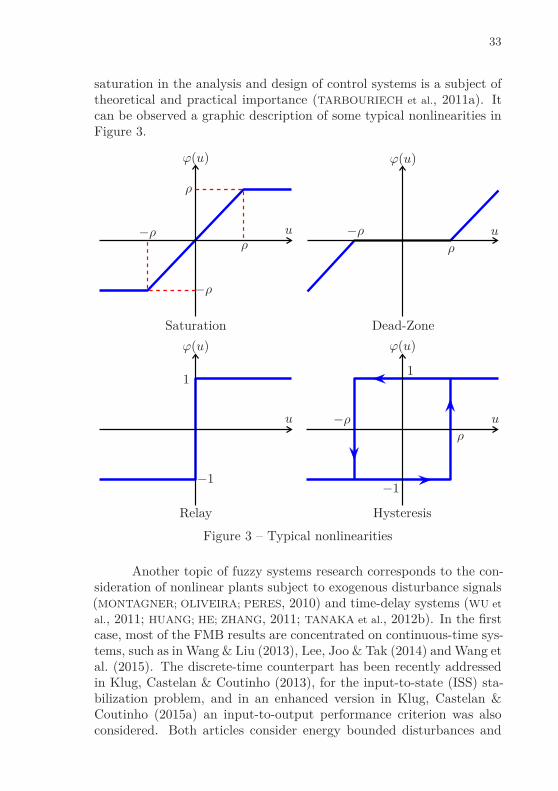
33
saturation in the analysis and design of control systems is a subject oftheoretical and practical importance (TARBOURIECH et al., 2011a). Itcan be observed a graphic description of some typical nonlinearities inFigure 3.
u
ϕ(u)
ρ
ρ−ρ
−ρ
Saturation
u
ϕ(u)
ρ
−ρ
Dead-Zone
u
ϕ(u)
1
−1
Relay
u
ϕ(u)
ρ−ρ
1
−1
Hysteresis
Figure 3 – Typical nonlinearities
Another topic of fuzzy systems research corresponds to the con-sideration of nonlinear plants subject to exogenous disturbance signals(MONTAGNER; OLIVEIRA; PERES, 2010) and time-delay systems (WU et
al., 2011; HUANG; HE; ZHANG, 2011; TANAKA et al., 2012b). In the firstcase, most of the FMB results are concentrated on continuous-time sys-tems, such as in Wang & Liu (2013), Lee, Joo & Tak (2014) and Wang etal. (2015). The discrete-time counterpart has been recently addressedin Klug, Castelan & Coutinho (2013), for the input-to-state (ISS) sta-bilization problem, and in an enhanced version in Klug, Castelan &Coutinho (2015a) an input-to-output performance criterion was alsoconsidered. Both articles consider energy bounded disturbances and

34
the local behavior of the design conditions. It should be emphasizedthat in the presence of amplitude bounded disturbances, the asymp-totic stability of the origin cannot be guaranteed and, in this case, theconcept of ultimate bounded (UB) stability is considered (i.e., the statetrajectory is guaranteed to converge to a region in the vicinity of thesystem origin). This problem is handled in the work Klug, Castelan &Coutinho (2015).
On the other hand, some recent results have addressed the FMBdynamic output feedback control problem such as in Zhang, Jiang &Staroswiecki (2010), Yoneyama (2014) and Nguyen, Dequidt & Dam-brine (2015), considering the premise variables to be available onlineto the controller. This assumption is noticeably restrictive, since thepremise variables vector is, in general, a nonlinear function of measu-rable and unmeasurable states (ASEMANI; MAJD, 2013). In Tognetti,Oliveira & Peres (2012) the problem of reduced-order dynamic outputfeedback control design for continuous-time systems is considered, usinga line-integral fuzzy Lyapunov function, allowing the membership func-tions to vary arbitrarily. The controller is obtained in a two-stage LMIprocedure with multi-simplex approach.
Finally, it is also important to highlight that the use of T-Sfuzzy models allows the systematic design with a numerical solution ofnonlinear control systems, whereas other techniques, such as feedbacklinearization, sliding-mode control, backstepping, passivity-based con-trol, among others, usually requires that the equations of the plant arepresented in a particular way and/or are only applied to a specific classof systems, besides having only analytic solutions. Thus, T-S fuzzy mo-dels provide an interesting framework for dealing with the fundamentalissues in modern control theory for complex nonlinear systems.
1.2 OBJECTIVES
Overall, a fundamental issue that must be solved in T-S fuzzycontroller design applied to nonlinear systems is concerning the restric-tions imposed either by the modeling process, related to the regionalvalidity of the model, or by the inherent physical constraints of actua-tors. Also, the presence of external signals usually found in real systemsshould be considered. In this context, the following specific objectivescan be established:
• Define a theoretical and algorithmic framework to take into ac-count the regional validity of the T-S fuzzy models in the nonli-
35
near control systems design, using the Lyapunov stability theoryfor building contractive sets in order to estimate the domain ofattraction of the closed-loop system (compute stability regions);
• Standardize a modeling process that provides a reduced numberof rules and consequently a decrease in the numerical complexityof the control algorithms, allowing also to handle the dynamicoutput feedback control problem for systems with nonlinearitiesthat may depend on unmeasurable states. This modeling processis based on the use of T-S fuzzy models with nonlinear local rules,referred to in this work as N-Fuzzy models;
• Develop conditions to synthesize controllers with guaranteed per-formance for nonlinear systems represented by N-fuzzy models,considering their regional validity and providing estimates of thestability region and admissible disturbance set, such as the onesbounded in energy and/or bounded in amplitude;
• Perform Hardware-in-the-Loop (HIL) simulations considering thephysical plant virtually emulated using a computer and the con-trollers embedded in a real programmable platform, in order toanalyze the complexity of digital implementation of classical andN-fuzzy controllers; and
• Provide an interactive tool for the scientific community of therelated area aiming to assist those users in the nonlinear controldesign using fuzzy strategies.
Specifically this thesis considers only nonlinear discrete-time sys-tems, not covering the discretization process for obtaining it. This im-portant aspect is a future perspective of this work in order to performreal implementations of the obtained theoretical results.
1.3 STRUCTURE OF THE THESIS
This document is organized as follows:In Chapter 2 some fundamental concepts are presented on Takagi-
Sugeno fuzzy systems with nonlinear local rules, as well as the associ-ated modeling process, discussions concerning the regional validity anda comparison of the numerical complexity involving classical and N-fuzzy models. It is important to emphasize the flexibility provided byN-fuzzy modeling, allowing the control designer to conveniently modify

36
the control law in relation to the vector of sector nonlinearities, enablingfor instance the practical implementation of fuzzy dynamic controllers.
Chapters 3, 4 and 5 are composed of the main contributions ofthis thesis, the results of which have been published or submitted innational and international conferences and journals. These chaptersdeal with, respectively: i) dynamic output feedback control design fornonlinear systems with saturating actuators represented by T-S fuzzymodels; ii) the input-to-state stabilization problem with a certain input-to-output performance for nonlinear systems subject to energy boundeddisturbances; and iii) ultimate bounded stabilization for nonlinear sys-tems subject to amplitude bounded disturbances using state and dy-namic output feedback in a special configuration that allows the pre-sence of unmeasurable nonlinearities. In all cases the inherent localcharacteristic of T-S modeling technique is taken into consideration inthe design phase, ensuring that the closed-loop trajectories evolve onlyin the T-S domain of validity.
Chapter 6 deals with the development of a user-friendly stabilityanalysis and control design tool with interactive properties. This allowsthe user to, in a few steps, obtain a reasonable controller for a knownnonlinear system that meets some desired closed-loop performance re-quirements. This chapter also presents practical aspects for implemen-ting T-S fuzzy controllers, analyzed from hardware-in-the-loop simula-tions using a Field Programmable Gate Array (FPGA) developmentboard.
In Chapter 7 some conclusions and recommendations for futureresearch are discussed. The appendices present some additional infor-mation which complements the understanding of the preceding chap-ters.

2 T-S FUZZY MODELS, RULE REDUCTION ANDREGIONAL VALIDITY
The objectives of this chapter are: formalize the mathematicaldescription of the T-S fuzzy models and present the N-fuzzy modelingprocess; compare the numerical complexity of the control algorithmsand the number of rules required in exact modeling for classical and N-fuzzy approaches; and analyze the modeling error and convexity on theexterior of the domain of validity. It is important to emphasize thatthe classical T-S fuzzy models described in Tanaka & Wang (2001)and Feng (2010) can be seen as a particular case of the N-fuzzy tech-nique addressed in this work, which will be explained later. Finally,it is presented the N-fuzzy models of some nonlinear plants used inthe remainder of this document, whose modeling process are show inAppendix B.
2.1 T-S FUZZY REPRESENTATION
The T-S fuzzy model, originally proposed by Takagi & Sugeno(1985), represents a nonlinear dynamic system by means of a fuzzy dy-namic model. This model consists of a set of local linear (or affine)submodels that are connected using membership functions. In this sec-tion, the discrete-time representation with nonlinear local submodels,also referred to as N-fuzzy, will be used. The modeling procedure andnotation are based in the article Klug & Castelan (2011).
Consider the class of nonlinear systems with state space repre-sentation affine in the input and disturbance signals, defined by thefollowing equation
x(k + 1) = f(x(k)) + V (x(k))u(k) + T (x(k))w(k)y(k) = Cx(k)
(2.1)
where x(k) ∈ X ⊂ ℜnx , u(k) ∈ U ⊂ ℜnu , y(k) ∈ Y ⊂ ℜny andw(k) ∈ W ⊂ ℜnw are respectively the state, the control input, thesystem output and the exogenous disturbance vectors. The functionsf(·) : ℜnx −→ ℜnx , with f(0) = 0, V (·) : ℜnx −→ ℜnx×nu andT (·) : ℜnx −→ ℜnx×nw are continuous and bounded for all x(k) ∈ X ,with X being a region belonging to the state space domain containingthe origin which will be defined later in this chapter. Furthermore, inorder to obtain numerically tractable conditions, the output vector y(k)
38
is considered to be linear, that is C ∈ ℜny×nx is a constant matrix.For a given nonlinear system as in (2.1), the N-fuzzy model is
represented by a description of IF-THEN fuzzy rules that express localdynamics by nonlinear local submodels, having R1, . . . , Rnr
fuzzy rulesdefined as follows
Rii=1,...,nr
:
IF ν(1)(k) is M i1, ν(2)(k) is M i
2, . . . , ν(ns)(k) is M ins
THENx(k + 1) = Aix(k)+Biu(k)+Bwiw(k)+Giϕ(k)
y(k) = Cx(k)(2.2)
with ν(k) := [ν(1)(k), ν(2)(k), ..., ν(ns)(k)] representing the premise vari-ables, M i
j , j = 1, . . . , ns, representing the fuzzy sets, and (Ai, Bi, Bwi,Gi, C) representing the matrices that define the fuzzy local submodels.The vector ϕ(k) = ϕ(π(k)) ∈ ℜnϕ , with π(k) = Lx(k), ϕ(0) = 0 andL ∈ ℜnϕ×nx , is a known nonlinear function of x(k) satisfying a (local)cone sector condition ϕ(·) ∈ S[0, Ω] for all x(k) ∈ X ⊂ ℜnx , i.e., amatrix 0 < Ω = Ω′ ∈ ℜnϕ×nϕ exists such that
ϕ′
(k)∆−1[ϕ(k) − ΩLx(k)] ≤ 0, ∀ x(k) ∈ X (2.3)
where ∆ ∈ ℜnϕ×nϕ is any positive diagonal matrix, that is, ∆ ,
diagδf , δf > 0, f = 1, . . . , nϕ. Ω is assumed to be a known parame-ter. From the definition of ∆, if (2.3) is verified then nϕ independentclassical conditions, ϕ′
(f)(k)[ϕ(k) − ΩLx(k)](f) ≤ 0, are also assured(JUNGERS; CASTELAN, 2011). Thus, ∆ represents a degree of freedomfor the purpose of design and optimization. Notice that if ϕ(k) = 0,then the rules R1, . . . , Rnr
recover the classical definition of T-S fuzzymodels (TAKAGI; SUGENO, 1985).
Let µij(ν(j)(k)) be the “weight” of the fuzzy set M i
j associated
to the premise variable ν(j)(k), and ωi(ν(k)) =ns∏
j=1
µij(ν(j)(k)). Consi-
dering µij(ν(j)(k)) ≥ 0, it follows that
ωi(ν(k)) ≥ 0, ∀ i = 1, ..., nr andnr∑
i=1
ωi(ν(k)) > 0.
Furthermore, the normalized weight of each rule, h(i)(k), alsoreferred to as the membership function of ith local submodel, satisfies:

39
h(i)(k) = h(ν(i)(k)) =ωi(ν(k))
nr∑
i=1
ωi(ν(k))
, ∀ i = 1, ..., nr, (2.4)
and it is limited in the unit simplex
Ξ =
h ∈ ℜnr ;nr∑
i=1
h(i) = 1, h(i) ≥ 0, i = 1, ..., nr
.
As will be clarified in the next section, the domain X and the simplexΞ are associated by the relation: x(k) ∈ X ⇒ h(i)(k) ∈ Ξ.
Thus, given (x(k), u(k), w(k), ϕ(k), ν(k)), the resulting fuzzy sys-tem is obtained as the weighted average of the local submodels (LEEK-
WIJCK W. V. AMD KERRE, 1999), also known as the center of gravitydefuzzification method. Therefore, it is obtained
x(k + 1) = A(h(k))x(k)+B(h(k))u(k)+Bw(h(k))w(k)+G(h(k))ϕ(k)y(k) = Cx(k)
(2.5)with the structure of the matrices given by
[
A(h(k)) B(h(k)) Bw(h(k)) G(h(k))]
=nr∑
i=1
h(i)(k)[
Ai Bi Bwi Gi
]
.
Notice that the fuzzy model (2.5) is equivalent to the represen-tation of a Lur’e type parameter varying system, referred to in thiswork as Nonlinear Parameter Varying (NPV) system, with polytopicuncertainties and cone bounded sector nonlinearities. This fact allowsfor stability analysis and control design techniques, originally proposedfor associated parameter varying systems, to be adapted for the use innonlinear systems that can be modeled using the N-fuzzy approach.
2.2 CONSTRUCTION OF THE FUZZY MODEL
In order to synthesize a fuzzy controller for a nonlinear plant, itis first necessary to obtain a T-S fuzzy model of this system. There-fore, the construction of a fuzzy model represents an important andbasic procedure when using Fuzzy Model Based (FMB) techniques. Ingeneral, there are two approaches for this purpose (TANAKA; WANG,2001):
40
1. identification using input-output data, and
2. derivation from given nonlinear system equations.
The approach using identification is suitable for plants that areunable or too difficult to be represented by analytical and/or physicalmodels. On the other hand, when the nonlinear analytical equationsare well-defined, for example in mechanical systems obtained by theLagrange method or Newton-Euler method, the second approach isused. This work focuses on the second case, using the exact modeling.
For the construction of approximate models, as in the methodshown in Teixeira & Zak (1999) (see Appendix A), the control designershould define operating points in the state space (based on the realbehavior of the nonlinear plant to be analyzed), which will be associ-ated with local linear submodels. These submodels can be determinedby optimization methods or by Taylor series. However, it should beemphasized that control systems designed using approximate modelscannot guarantee the performance and stability requirements initiallyestablished when applied to the original nonlinear plant, unless the dis-crepancies between the model and the plant are possible to be takeninto account in the design process or by further analysis.
2.2.1 Class of Nonlinear Systems
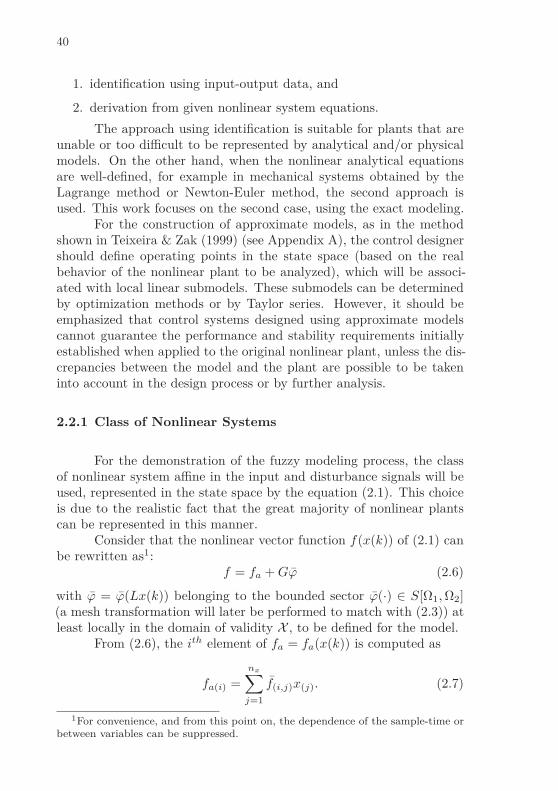
For the demonstration of the fuzzy modeling process, the classof nonlinear system affine in the input and disturbance signals will beused, represented in the state space by the equation (2.1). This choiceis due to the realistic fact that the great majority of nonlinear plantscan be represented in this manner.
Consider that the nonlinear vector function f(x(k)) of (2.1) canbe rewritten as1:
f = fa + Gϕ (2.6)
with ϕ = ϕ(Lx(k)) belonging to the bounded sector ϕ(·) ∈ S[Ω1, Ω2](a mesh transformation will later be performed to match with (2.3)) atleast locally in the domain of validity X , to be defined for the model.
From (2.6), the ith element of fa = fa(x(k)) is computed as
fa(i) =nx∑
j=1
f(i,j)x(j). (2.7)
1For convenience, and from this point on, the dependence of the sample-time orbetween variables can be suppressed.
41
Applying a similar procedure to V u=V (x(k))u(k), T w=T (x(k))w(k)and Gϕ=G(x(k))ϕ(k), the following is obtained
(V u)(i) =nu∑
κ=1
v(i,κ)u(κ), (T w)(i) =nw∑
l=1
t(i,l)w(l)
and (Gϕ)(i) =
nϕ∑
o=1
g(i,o)ϕ(o). (2.8)
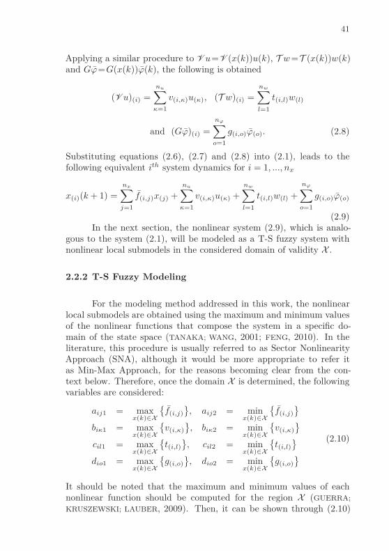
Substituting equations (2.6), (2.7) and (2.8) into (2.1), leads to thefollowing equivalent ith system dynamics for i = 1, ..., nx
x(i)(k + 1) =nx∑
j=1
f(i,j)x(j) +nu∑
κ=1
v(i,κ)u(κ) +nw∑
l=1
t(i,l)w(l) +
nϕ∑
o=1
g(i,o)ϕ(o)
(2.9)In the next section, the nonlinear system (2.9), which is analo-
gous to the system (2.1), will be modeled as a T-S fuzzy system withnonlinear local submodels in the considered domain of validity X .
2.2.2 T-S Fuzzy Modeling
For the modeling method addressed in this work, the nonlinearlocal submodels are obtained using the maximum and minimum valuesof the nonlinear functions that compose the system in a specific do-main of the state space (TANAKA; WANG, 2001; FENG, 2010). In theliterature, this procedure is usually referred to as Sector NonlinearityApproach (SNA), although it would be more appropriate to refer itas Min-Max Approach, for the reasons becoming clear from the con-text below. Therefore, once the domain X is determined, the followingvariables are considered:
aij1 = maxx(k)∈X
f(i,j)
, aij2 = minx(k)∈X
f(i,j)
biκ1 = maxx(k)∈X
v(i,κ)
, biκ2 = minx(k)∈X
v(i,κ)
cil1 = maxx(k)∈X
t(i,l)
, cil2 = minx(k)∈X
t(i,l)
dio1 = maxx(k)∈X
g(i,o)
, dio2 = minx(k)∈X
g(i,o)
(2.10)
It should be noted that the maximum and minimum values of eachnonlinear function should be computed for the region X (GUERRA;
KRUSZEWSKI; LAUBER, 2009). Then, it can be shown through (2.10)
42
that it is possible to represent f(i,j), v(i,κ), t(i,l) and g(i,o) as
f(i,j) =2∑
ℓa=1
αijℓa(x(k))aijℓa v(i,κ) =2∑
ℓb=1
βiκℓb(x(k))biκℓb
t(i,l) =2∑
ℓc=1
γilℓc(x(k))cilℓc g(i,o) =2∑
ℓd=1
δioℓd(x(k))dioℓd
(2.11)
with
αij1 =f(i,j) − aij2
aij1 − aij2, αij2 =
aij1 − f(i,j)
aij1 − aij2,
βiκ1 =v(i,κ) − biκ2
biκ1 − biκ2, βiκ2 =
biκ1 − v(i,κ)
biκ1 − biκ2,
γil1 =t(i,l) − cil2
cil1 − cil2, γil2 =
cij1 − t(i,l)
cil1 − cil2,
δio1 =g(i,o) − dio2
dio1 − dio2and δio2 =
dio1 − g(i,o)
dio1 − bio2.
(2.12)
Notice that
2∑
ℓa=1
αijℓa =2∑
ℓb=1
βiκℓb =2∑
ℓc=1
γilℓc =2∑
ℓd=1
δioℓd = 1. (2.13)
It is also observed that ℓa, ℓb, ℓc and ℓd are associated with the ex-tremum points (maximum and minimum) of nonlinear functions in thedomain X . Substituting (2.11) into (2.9), leads to
x(i)(k + 1)=nx∑
j=1
2∑
ℓa=1
αijℓa(x(k))aijℓax(j)+nu∑
κ=1
2∑
ℓb=1
βiκℓb(x(k))biκℓbu(κ)
+nw∑
l=1
2∑
ℓc=1
γilℓc(x(k))cilℓcw(l)+
nϕ∑
o=1
2∑
ℓd=1
δioℓd(x(k))dioℓd ϕ(o)
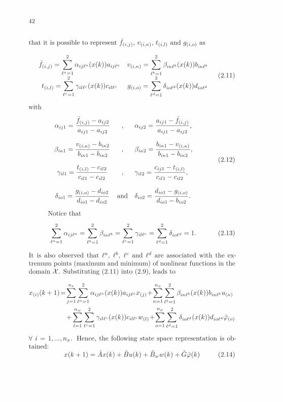
∀ i = 1, ..., nx. Hence, the following state space representation is ob-tained:
x(k + 1) = Ax(k) + Bu(k) + Bww(k) + Gϕ(k) (2.14)

43
with
N =
2∑
ℓn=1
η11ℓnn11ℓn · · ·2∑
ℓn=1
η1nxℓnn1nxℓn
.... . .
...2∑
ℓn=1
ηnx1ℓnnnx1ℓn · · ·2∑
ℓn=1
ηnxnxℓnnnxnxℓn
where the tuple (N , η, n, ℓn) represents either(
A, α, a, ℓa)
,(
B, β, b, ℓb)
,(
Bw, γ, c, ℓc)
or(
G, δ, d, ℓd)
.From the summation property in (2.13), the expression (2.14)
can be conveniently rewritten by swapping the summations indices asfollows
x(k + 1) =2∑
p11=1
...
2∑
pnxnx =1
2∑
q11=1
...
2∑
qnxnu =1
2∑
r11=1
...
2∑
rnxnw =1
2∑
s11=1
...
2∑
snxnϕ =1
hp,q,r,s(Apx + Bqu + Bwrw + Gsϕ)(2.15)
with
Ap =
a11p11· · · a1nxp1nx
.... . .
...anx1pnx1
· · · anxnxpnxnx
,
Bq =
b11q11· · · b1nuq1nu
.... . .
...bnx1qnx1
· · · bnxnuqnxnu
,
Bwr =
c11r11· · · c1nwr1nw
.... . .
...cnx1rnx1
· · · cnxnwrnxnw
,
Gs =
d11o11· · · d1nϕo1nϕ
.... . .
...dnx1onx1
· · · dnxnϕonxnϕ
,
and
hp,q,r,s =α11p11...αnxnxpnxnx
β11q11...βnxnuqnxnu
γ11r11...γnxnwqnxnw
δ11r11...δnxnϕqnxnϕ
.

44
Then, aggregating the summations and performing a mesh trans-formation (see Appendix C) with the nonlinearity ϕ leads to
x(k +1) =2
∑
i=1
h(i)(k) Aix(k) + Biu(k) + Bwiw(k) + Giϕ(k), (2.16)
where h(i)(k) = hp,q,r,s, = nxnx + nxnu + nxnw + nxnϕ, Ai =Ai + GiΩ1L, Bi = Bi, Bwi = Bwi, Gi = Gi e ϕ = ϕ − Ω1Lx, withϕ(.) ∈ S[0 Ω].
The equation (2.16) represents the T-S fuzzy model with nonli-near local rules described in (2.5), where Ai, Bi, Bwi and Gi are depen-dent on the extremum values aijℓa , biκℓb , cilℓc and dioℓd of the nonline-arities of the system. The membership functions h(i)(k) are dependenton the functions αijℓa(x(k)), βiκℓb(x(k)), γilℓc(x(k)) and δioℓd(x(k)) de-fined in (2.12), and correspond to time-varying parameters for a NPVpolytopic system.
Based on the aforementioned N-fuzzy modeling technique, andin other methods found in literature, an important issue usually notconsidered by researchers is that to obtain numerically tractable solu-tions for the stability analysis and control design of nonlinear systems,the available T-S fuzzy modeling techniques can only locally guaran-tee the stability properties of the original nonlinear system. Noticewhen deriving a T-S fuzzy model that a normalizing step is used in thedefuzzification process, which requires that the premise variables arebounded in some chosen compact set, i.e. the positiveness of the func-tions in (2.12), and consequently of the membership functions h(i)(k),it is only guaranteed if x(k) ∈ X .
In light of the above, there exists a bounded region X of statespace containing the origin such that x(k) ∈ X ⇒ h(i)(k) ∈ Ξ. Hence,when applying convex methods to solve fuzzy based stability conditionson the Ξ space, it is necessary to take into account that the stabilityconditions hold only if the state trajectory of the original nonlinearsystem does not leave X . From this reasoning, we refer to the regionX as the T-S domain of validity. In this work, the domain X will bedefined by means of the following polyhedral set
X = x(k) ∈ ℜnx : |Nx(k)| φ, (2.17)
where φ ∈ ℜnφ and N ∈ ℜnφ×nx are given constants. Also, φ representsthe bounds of the associated states, and nφ ≤ nx represents the numberof constraints characterizing the region X . For example, considering ageneric nonlinear system with x(k) ∈ ℜ3, and the limits
∣
∣x(1)(k)∣
∣ ≤ 2

45
and∣
∣x(2)(k)∣
∣ ≤ 3, with the free state x(3)(k), the domain X in (2.17)can be characterized by
N =
[
1 0 00 1 0
]
and φ =
[
23
]
.
This domain of validity should be taken into account in anycontrol design or stability analysis that assumes the description (2.16)instead of (2.1) and is based on convex properties of the N-fuzzy model.Specifically, loss of performance or even instability may occur whenthe state trajectory evolves outside the domain of validity of the model(2.16).
Remark 2.1 For the classical T-S fuzzy modeling described in Tanaka& Wang (2001), the vector of sector nonlinearities ϕ does not explicitlyappear in the model equation (2.16). Otherwise, these nonlinearitiesshould be handled and indirectly included in the system state matrix,as shown in the sequel. Let the unidimensional discrete-time nonlinearsystem
x(k + 1) = fa(x(k)) + 0.7ϕ(k) + u(k) + 0.2w(k),
with ϕ = ϕ(Lx) = sin(x), L = 1, and fa = x2 = fx ⇒ f = x.Considering that the trajectories are restricted to the state space domaindefined by |x| ≤ π/2, it is possible to rewrite f , following the steps
(2.10), (2.11) and (2.12), by f =2∑
ℓa=1
αℓaaℓa , with a1 = π/2, a2 =
−π/2, α1 =x − a2
a1 − a2and α2 =
a1 − x
a1 − a2. It can also be observed that
the nonlinearity ϕ is bounded in the sector ϕ ∈ S[Ω1, Ω2], with Ω1 = 2/πand Ω2 = 1. Thus, the T-S fuzzy model with nonlinear local rules isgiven by
x(k + 1) =2∑
ℓa=1
αℓa(k) aℓax(k) + u(k) + 0.2w(k) + 0.7ϕ(k). (2.18)
with the membership functions h(i)(k) = α(i)(k), i = 1, 2, depicted inFigure 4.
In another way, it is possible to rewrite the nonlinearity ϕ, inthe considered state space domain, as
ϕ = sin(x) =
(
2∑
ℓe=1
ǫℓeΩℓe
)
x, (2.19)

46
−1.5 −1 −0.5 0 0.5 1 1.5
0
0.2
0.4
0.6
0.8
1
x(k)
h(i
)(k
)
h(1)h(2)
−π/2 π/2
Figure 4 – Membership functions h(i)(k) for N-fuzzy model
where ǫℓe = ǫℓe(x(k)), ℓe = 1, 2, are any functions that satisfy (2.19)and respect the properties ǫ1 +ǫ2 = 1 and ǫℓe ≥ 0, ℓe = 1, 2, ∀ x(k) ∈ X .One possibility is to choose
ǫ1 =
sin(x) − Ω1x
x(Ω2 − Ω1), x 6= 0
1, x = 0and ǫ2 =
Ω2x − sin(x)
x(Ω2 − Ω1), x 6= 0
0, x = 0
Hence, it has the following classical T-S fuzzy model with linear localrules
x(k + 1) =2∑
ℓa=1
2∑
ℓe=1
αℓa(k)ǫℓe(k) (aℓa +0.7Ωℓe)x(k)+u(k)+0.2w(k)
=4∑
i=1
h(i)(k) Aix(k)+u(k)+0.2w(k)
(2.20)with Ai = aℓa +0.7Ωℓe and h(i)(k) = αℓa(k)ǫℓe(k), for i = ℓe +2(ℓa −1)and ℓa, ℓe = 1, 2. It is worth noting that the term Ωℓe
in (2.20), relatedto the sector nonlinearity, appears attached to the system state matrix.Furthermore, the treatment of ϕ implies an additional summation, andconsequently an increase in the number of local submodels. This factorwill be further explored in the next subsection.
In Figure 5 the membership functions h(i)(k) for the model (2.20)are depicted. As in the Figure 4, the reader can notice that the mem-
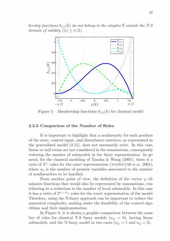
47
bership functions h(i)(k) do not belong to the simplex Ξ outside the T-Sdomain of validity (|x| ≤ π/2).
−1.5 −1 −0.5 0 0.5 1 1.5
0
0.2
0.4
0.6
0.8
1
x(k)
h(i
)(k
)
h(1)h(2)h(3)h(4)
−π/2 π/2
Figure 5 – Membership functions h(i)(k) for classical model
2.2.3 Comparison of the Number of Rules
It is important to highlight that a nonlinearity for each positionof the state, control input, and disturbance matrices, as represented inthe generalized model (2.15), does not necessarily exist. In this case,linear or null terms are not considered in the summations, consequentlyreducing the number of submodels in the fuzzy representation. In ge-neral, for the classical modeling of Tanaka & Wang (2001), there is aratio of 2ns rules for the exact representation (TANIGUCHI et al., 2001),where ns is the number of premise variables associated to the numberof nonlinearities to be handled.
From another point of view, the definition of the vector ϕ eli-minates functions that would also be represented by summations, con-tributing to a reduction in the number of local submodels. In this caseit has a ratio of 2ns−nϕ rules for the exact representation of the model.Therefore, using the N-fuzzy approach can be important to reduce thenumerical complexity, making easier the feasibility of the control algo-rithms and their implementation.
In Figure 6, it is shown a graphic comparison between the num-ber of rules for classical T-S fuzzy models (nϕ = 0), having linearsubmodels, and the N-fuzzy model in two cases (nϕ = 1 and nϕ = 2).

48
1 2 3 4 5 60
10
20
30
40
50
60
70
Number of nonlinearities(ns)
Num
ber
ofru
les
(2n
s,2
ns−
nϕ) nϕ = 0
nϕ = 1nϕ = 2
Figure 6 – Comparison of the number of rules
Notice that the larger is the size of the vector ϕ, the greater isthe reduction of rules, after all 2ns−nϕ = 2ns/2nϕ . This relation allowsto check a division factor of 2nϕ in relation to the classical T-S fuzzymodel.
2.3 MODELING ERROR ANALYSIS AND REGIONAL VALIDITY
An important issue when dealing with the T-S fuzzy models con-sidered in the present work is that the convexity can only be guaranteedin a specific region of the state space, referred to as the domain of va-lidity X . The exception is for systems whose sector nonlinearities canbe globally encompassed and/or a global maximum/minimum can befound. Otherwise, it is necessary to assign a confined region to com-pute the extremum points and/or to find a local bounded sector forthe nonlinearities of the system. However, provided that the stabilityconditions are properly handled, this may not be a serious problem,because most real systems already have physical limitations which na-turally constraint the excursion of the states.
Nonetheless, the inherent local characteristic of T-S modelingtechniques is often not considered in most FMB control design results,as can be observed in Tognetti & Oliveira (2009), Andrea et al. (2008),Yang & Yang (2012), Mozelli & Palhares (2011a) and in references

49
therein. Hence, the synthesized control laws in these references basedon convex methods may lead to trajectories of the controlled nonli-near system evolving outside the domain of validity, thus representinga source of performance degradation or even instability of the corres-ponding closed-loop system.
As previously discussed, the loss of model convexity is associ-ated with the positiveness of the membership functions, which is onlyensured for the domain X . A common strategy employed to avoidh(k) /∈ Ξ, ∀ x(k) /∈ X is to partition the membership functions h(i)(k)in order to saturate them, i.e. h(i)(k) ∈ [0, 1]. In other words, if thevalue of h(i)(k) is greater than 1, it is set (“clipped”) to 1, if the valueof h(i)(k) is lower than 0, it is set (“clipped”) to 0. This strategy,despite its success when applied to the T-S fuzzy model, introducesmodeling errors that might result in similar issues observed for the lossof model convexity case, when applied to the original nonlinear system.To sum up, in practical applications either the membership functionare clipped, in which the model convexity is preserved at the cost ofmodeling errors, or not clipped, in which the model convexity is lost butthe fuzzy model is exact. The following examples aim to demonstratethe involved problematic.
Example 2.2 (Modeling Error) Let the nonlinear function f(x) =x sin2(x), with x ∈ ℜ. It is desired to obtain an exact T-S fuzzy modelof the function using the procedures described in the subsection 2.2.2.For this purpose, the domain of validity is considered (for example dueto physical limitations) as X = x ∈ ℜ : |x| ≤ π/3. Computing themaximum and minimum values of the nonlinear function f(x) for Xleads to
a1 = maxx∈X
f(x)
= 0.7854, and a2 = minx∈X
f(x)
= −0.7854.
Thus, it is possible to rewrite f(x), using (2.11) and (2.12), as thefollowing equivalent T-S fuzzy model
f(x) =2∑
ℓa=1
αℓa(f(x))aℓa , ∀ x ∈ X , (2.21)
with
α1(f(x)) =
f(x) − a2
a1 − a2, a2 ≤ f(x) ≤ a1
1, f(x) > a1
0, f(x) < a2
and
50
α2(f(x)) =
a1 − f(x)
a1 − a2, a2 ≤ f(x) ≤ a1
0, f(x) > a1
1, f(x) < a2
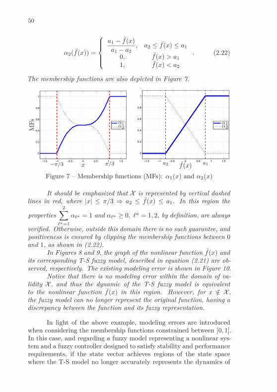
. (2.22)
The membership functions are also depicted in Figure 7.
−1.5 −1 −0.5 0 0.5 1 1.5
0
0.2
0.4
0.6
0.8
1
x
MF
s
α1α2
−π/3 π/3−1.5 −1 −0.5 0 0.5 1 1.5
0
0.2
0.4
0.6
0.8
1
f(x)a2 a1
α1α2
Figure 7 – Membership functions (MFs): α1(x) and α2(x)
It should be emphasized that X is represented by vertical dashedlines in red, where |x| ≤ π/3 ⇒ a2 ≤ f(x) ≤ a1. In this region the
properties
2∑
ℓa=1
αℓa = 1 and αℓa ≥ 0, ℓa = 1, 2, by definition, are always
verified. Otherwise, outside this domain there is no such guarantee, andpositiveness is ensured by clipping the membership functions between 0and 1, as shown in (2.22).
In Figures 8 and 9, the graph of the nonlinear function f(x) andits corresponding T-S fuzzy model, described in equation (2.21) are ob-served, respectively. The existing modeling error is shown in Figure 10.
Notice that there is no modeling error within the domain of va-lidity X , and thus the dynamic of the T-S fuzzy model is equivalentto the nonlinear function f(x) in this region. However, for x /∈ X ,the fuzzy model can no longer represent the original function, having adiscrepancy between the function and its fuzzy representation.
In light of the above example, modeling errors are introducedwhen considering the membership functions constrained between [0, 1].In this case, and regarding a fuzzy model representing a nonlinear sys-tem and a fuzzy controller designed to satisfy stability and performancerequirements, if the state vector achieves regions of the state spacewhere the T-S model no longer accurately represents the dynamics of

51
−1.5 −1 −0.5 0 0.5 1 1.5
−1.5
−1
−0.5
0
0.5
1
1.5
x(k)
f(x
)
Figure 8 – Nonlinear function
−1.5 −1 −0.5 0 0.5 1 1.5
−1.5
−1
−0.5
0
0.5
1
1.5
x(k)
∑
2 ℓa
=1
αℓ
aa
ℓa
Figure 9 – T-S fuzzy representation
−1.5 −1 −0.5 0 0.5 1 1.5
−1.5
−1
−0.5
0
0.5
1
1.5
x(k)
Err
or
Figure 10 – Modeling error when MFs are clipped for x(k) /∈ X
52
the original plant, the desired stability and performance may not beguaranteed for the original system.
In the following, an illustrative example aims to demonstrate theproblems that may occur in practice when the inherent local characte-ristic of T-S modeling techniques are not considered in control design,either by modeling error introduced when restricting the membershipfunctions, or because of the loss of model convexity outside the domainX .
Example 2.3 (Local Stability) For simplicity, consider the follo-wing unidimensional nonlinear discrete-time system without control sa-turation constraints (KLUG et al., 2014)
x(k+1) = x3(k)+sin(x(k))+(0.2+x2(k))u(k) , y(k) = x(k) (2.23)
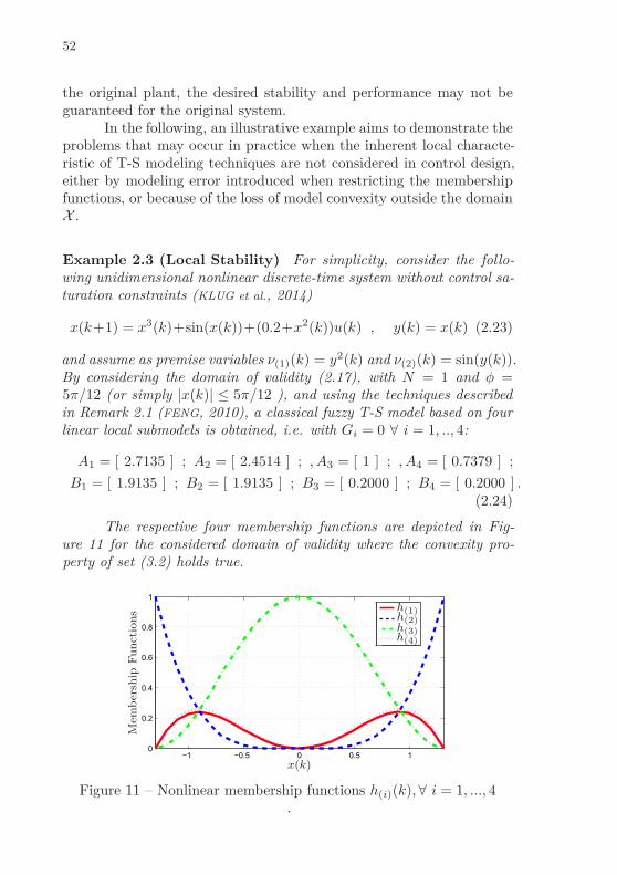
and assume as premise variables ν(1)(k) = y2(k) and ν(2)(k) = sin(y(k)).By considering the domain of validity (2.17), with N = 1 and φ =5π/12 (or simply |x(k)| ≤ 5π/12 ), and using the techniques describedin Remark 2.1 (FENG, 2010), a classical fuzzy T-S model based on fourlinear local submodels is obtained, i.e. with Gi = 0 ∀ i = 1, .., 4:
A1 = [ 2.7135 ] ; A2 = [ 2.4514 ] ; , A3 = [ 1 ] ; , A4 = [ 0.7379 ] ;
B1 = [ 1.9135 ] ; B2 = [ 1.9135 ] ; B3 = [ 0.2000 ] ; B4 = [ 0.2000 ] .(2.24)
The respective four membership functions are depicted in Fig-ure 11 for the considered domain of validity where the convexity pro-perty of set (3.2) holds true.
−1 −0.5 0 0.5 10
0.2
0.4
0.6
0.8
1
h(1)h(2)h(3)h(4)
x(k)
Mem
ber
ship
Fu
nct
ion
s
Figure 11 – Nonlinear membership functions h(i)(k), ∀ i = 1, ..., 4.
53
These functions are the binary product between functions M ij ,
j = 1, 2 and i = 1, 2, defined as:
M11 =
x2
1.7135, M1
2 =−x2
1.7135, and
M21=
sin(x) − 0.7379x
x(0.2621), x 6= 0
1, x = 0, M2
2=
x − sin(x)
x(0.2621), x 6= 0
0, x = 0.
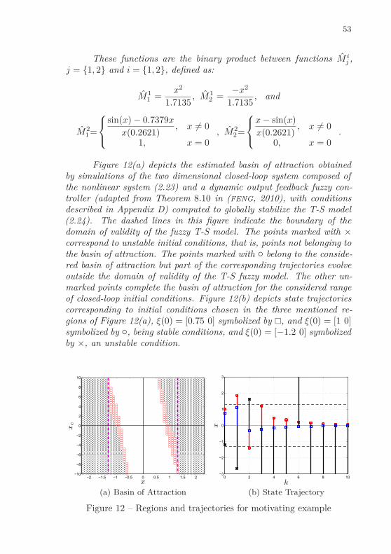
Figure 12(a) depicts the estimated basin of attraction obtainedby simulations of the two dimensional closed-loop system composed ofthe nonlinear system (2.23) and a dynamic output feedback fuzzy con-troller (adapted from Theorem 8.10 in (FENG, 2010), with conditionsdescribed in Appendix D) computed to globally stabilize the T-S model(2.24). The dashed lines in this figure indicate the boundary of thedomain of validity of the fuzzy T-S model. The points marked with ×correspond to unstable initial conditions, that is, points not belonging tothe basin of attraction. The points marked with belong to the conside-red basin of attraction but part of the corresponding trajectories evolveoutside the domain of validity of the T-S fuzzy model. The other un-marked points complete the basin of attraction for the considered rangeof closed-loop initial conditions. Figure 12(b) depicts state trajectoriescorresponding to initial conditions chosen in the three mentioned re-gions of Figure 12(a), ξ(0) = [0.75 0] symbolized by , and ξ(0) = [1 0]symbolized by , being stable conditions, and ξ(0) = [−1.2 0] symbolizedby ×, an unstable condition.
−2 −1.5 −1 −0.5 0 0.5 1 1.5 2−10
−8
−6
−4
−2
0
2
4
6
8
10
x
xc
(a) Basin of Attraction
0 2 4 6 8 10−3
−2
−1
0
1
2
3
k
x
(b) State Trajectory
Figure 12 – Regions and trajectories for motivating example

54
It is remarkable, as shown in Figures 12, that a compensator thatin theory globally stabilizes the fuzzy T-S closed-loop system may yieldunstable trajectories even though the initial conditions are inside thedomain of validity when applied in the original nonlinear system (2.23).On the other hand, the use of some adequate techniques taking intoaccount the domain of validity issue prevents unstable initial conditionsinside a sub-region of X , as will be seen in the following chapters.
In this sense, the local stabilization of nonlinear systems usingT-S fuzzy models is an important contribution of this work, in whichefforts were devoted to estimate a safe domain of attraction, i.e. aregion of admissible initial conditions that asymptotically converge tothe origin, for the closed-loop system.
2.4 CONCLUDING REMARKS
In this chapter some general concepts of T-S fuzzy systems the-ory were presented. A generalized process of modeling with the use ofnonlinear local submodels, referred to as N-fuzzy modeling, was descri-bed. The objective is to obtain an exact representation of the nonlinearplant with the least possible number of rules, reducing the numericalcomplexity and consequently making easier the feasibility of the sub-sequently developed control algorithms and their practical implemen-tation. A comparative study of the number of rules for classical andN-fuzzy models was also performed. The important issue of regionalvalidity was discussed, generally disregarded by researchers in this area.At last, examples of nonlinear systems modeled by T-S fuzzy models aredetailed in Appendix B, and an analysis of the numerical complexityof control algorithms is presented in Appendix D .
3 DYNAMIC OUTPUT FEEDBACK CONTROLDESIGN
In this chapter a control design technique for discrete-time nonli-near systems that can be represented by the N-Fuzzy model describedin Chapter 2 is presented. The control law considered is a dynamicoutput feedback with some particularities which will be described later.Basically, the objective is to propose a systematic method for obtainingthe matrices of the controller, dealing with some key practical issuessuch as the saturation of the actuators and the regional validity of theT-S fuzzy model.
The proposed dynamic compensator is full-order and dependenton the fuzzy membership functions that are assumed to be availableonline to the controller. Additionally, anti-windup gains are added asan attempt to mitigate the undesired effects of saturation, and a per-formance index based on the λ-contractivity of the level set, associatedwith the Lyapunov function, is used in order to ensure a certain rateof temporal convergence of the closed-loop system trajectories. Theresults presented here are enhanced versions of the works Klug & Cas-telan (2012) and Klug et al. (2014).
The numerical results described in the present chapter and inthe next ones, were obtained using the following computational tools:
1. Yalmip (LöFBERG, 2004): an interface for the mathematical de-scription of the considered LMI-optimization problem and man-agement of the SDP-solver to be used;
2. SeDuMi (STURM, 1999) and SDPT3 (TOH; TUTUNCU; TODD, 2004):SDP-solvers which are used to search for feasible solutions of theLMI-based control algorithms;
3. Simulink: a graphical programming environment for modeling,simulating and analyzing multidomain dynamic systems.
3.1 PROBLEM FORMULATION
Consider the class of undisturbed nonlinear systems that can bemodeled by the process demonstrated in section 2.2, described using

56
the defuzzification method by center of gravity as follows:
x(k + 1) = A(h(k))x(k) + B(h(k))sat(u(k)) + G(h(k))ϕ(k)y(k) = Cx(k)
(3.1)where x(k) ∈ X ⊂ ℜnx , u(k) ∈ U ⊂ ℜnu and y(k) ∈ Y ⊂ ℜny arerespectively the state, the control input and the system output vectors.h(k) ⊂ ℜnr is a vector of time-varying membership functions, andlimited, ∀ x(k) ∈ X , in the unit simplex
Ξ =
h ∈ ℜnr ;nr∑
i=1
h(i) = 1, h(i) ≥ 0, i = 1, ..., nr
. (3.2)
The function sat(.) : ℜnu → ℜnu represents the saturation of the con-trol inputs, defined by the standard decentralized saturation function
sat(u(ℓ)(k)) = sign(u(ℓ)(k))min(ρ(ℓ),∣
∣u(ℓ)(k)∣
∣), ∀ ℓ = 1, ..., nu (3.3)
where ρ(ℓ) > 0 denotes the symmetric amplitude bound relative to theithcontrol input.
Complementing the fuzzy model description (3.1), the vector ofsector nonlinearities ϕ(k) = ϕ(π(k)) ∈ ℜnϕ , with π(k) = Ly(k) =Lx(k), L = LC ∈ ℜnϕ×nx , and L with appropriate dimensions, verifies(at least locally) the sector condition (2.3). This definition is requiredfor control purposes.
The matrix structure is given by
[
A(h(k)) B(h(k)) G(h(k))]
=nr∑
i=1
h(i)(k)[
Ai Bi Gi
]
.
(3.4)Once the premise variables vector ν(k) is assumed to be a func-
tion of the measurable states, i.e., ν(k) = ν(y(k)), the vector of mem-bership functions can be reconstituted in real-time from these signals.In other words, h(k) = h(ν(y(k))) = h(y(k)). This assumption is nece-ssary to implement any output feedback controller based on the PDCstrategy, in which the membership functions are shared between thefuzzy model and controller. Notice that many works in literature donot clarify this important property, even using examples that can notbe implemented in practice.
In light of the above, the following full-order nonlinear fuzzy

57
(N-fuzzy) dynamical output feedback compensator is investigated:
xc(k + 1) = Ac(h(k))xc(k) + Bc(h(k))y(k) + Gc(h(k))ϕ(Lx(k))−Ec(h(k))Ψ(u(k))
u(k) = Cc(h(k))xc(k) + Dc(h(k))y(k) + Fc(h(k))ϕ(Lx(k))(3.5)
where xc(k) ∈ ℜnx×nx and Ψ(.) : ℜnu → ℜnu is the dead-zone nonline-arity given by:
Ψ(u(k)) = u(k) − sat(u(k)), (3.6)
and the controller matrices are as follows[
Ac (h(k)) Bc (h(k)) Gc (h(k))]
=nr∑
i=1
nr∑
j=i
(1 + ςij)h(i)(k)h(j)(k)
[
Acij
2
Bcij
2
Gcij
2
]
(3.7)[
Cc (h(k)) Dc (h(k)) Fc (h(k)) Ec (h(k))]
=nr∑
i=1
h(i)(k)[
Cci Dci Fci Eci
]
,
with ςij a binary variable such that
ςij =
1 if i 6= j,0 otherwise.
(3.8)
As assumed in Arcak, Larsen & Kokotovic (2003), the feedback con-troller (3.5) requires either the knowledge of ϕ(·) or its availability asa signal whenever Gc(h(k)) 6= 0 or Fc(h(k)) 6= 0. In addition, Ec(h(k))is a fuzzy anti-windup gain matrix that helps to mitigate the effects ofthe saturation. It is worthwhile to say that such anti-windup gain isusually addressed as a constant and the present proposal may improvethe closed-loop behavior, once it may contains the time-invariant gain,E(h(k)) = Ec, as a special case.
Considering the augmented state vector ξ(k) = [x′
(k) x′
c(k)]′ ∈
ℜ2nx , the closed-loop system can be described by:
ξ(k + 1) = A(h(k))ξ(k) + G(h(k))ϕ(Lξ(k))
−B(h(k))Ψ(
K(h(k))ξ(k) + Fc(h(k))ϕ(π(k))) (3.9)
with
A(h(k)) =
[
A(h(k)) + B(h(k))Dc(h(k))C B(h(k))Cc(h(k))Bc(h(k))C Ac(h(k))
]
,
58
B(h(k)) =
[
B(h(k))Ec(h(k))
]
, G(h(k)) =
[
G(h(k)) + B(h(k))Fc(h(k))Gc(h(k))
]
,
K(h(k)) =[
Dc(h(k))C Cc(h(k))]
, and L =[
L 0]
.
In view to the regional validity defined by (2.17), the T-S domainof validity is redefined in terms of the augmented space:
X a = ξ(k) ∈ ℜ2nx : |Nξ(k)| φ, (3.10)
where N = [ N 0nφ×nx] ∈ ℜnφ×2nx .
Thus, the problem of designing a controller (3.5) such that theclosed-loop system remains stable requires handling the validity domain(3.10) besides a region of initial conditions ξ(0) such that the allowedamplitudes of control signals are sufficient to assure the origin of (2.1)as an asymptotically stable equilibrium point. Such region of initialconditions is noted here as S0 and consists of a subset of the domain ofattraction of the resulting nonlinear closed-loop system (2.1) (KHALIL,2003, Sec. 8.2). As discussed in Tarbouriech et al. (2008), the basinof attraction can be defined as the set of all ξ(k) such that for all ξ(0)belonging to such set the corresponding system’s trajectory convergesasymptotically to the origin. It is noteworthy that an exact characteri-zation of such set is in general not possible. This problem is formalizedin the sequel:
Problem 3.1 Determine the parameters of the controller (3.5), and aregion S0 ⊆ ℜ2nx , as large as possible, such that the origin of the closed-loop system (3.9) is asymptotically stable and for any initial conditionξ(0) ∈ S0, the corresponding trajectories of the closed-loop system re-main in X a.
Remark 3.2 The differentiated structure (3.7), proposed to matricesAc(·), Bc(·) and Gc(·), is required for obtaining the gains of the con-troller (3.5) from stabilizing conditions that will be proposed in the formof LMIs. Adopting a simplified structure, in this case, would invalidatethis procedure, but could be used for the design of a controller withCc(h(k)) = Cc, Dc(h(k)) = Dc and Fc(h(k)) = Fc.
Remark 3.3 An alternative to the structure (3.7) was used in theworks Klug & Castelan (2012) and Klug et al. (2014). This structureis based in a split of summations, generically represented by matrix J(.)as
J (h(k)) =nr∑
i=1
h(i)(k)2Ji +nr−1∑
i=1
nr∑
j=i+1
h(i)(k)h(j)(k)Jij

59
However, comparing the above representation with (3.7), it can be con-cluded that there exists an equivalence between the two structures inrespect to the number of controller matrices and to the numerical com-plexity of the subsequent control algorithms. Thus, for convenience, itwas used (3.7), since this provides a more compact representation.
It should be emphasized that the closed-loop matrices in (3.9)can be rewritten, by using the special structure (3.7) of the fuzzy com-pensator and some summation properties, as
[
A (hk) G (hk)]
=nr∑
i=1
nr∑
j=i
(1 + ςij)h(i)(k)h(j)(k)
[
Aij
2
Gij
2
]
with
Aij =
[
Ai + Aj + (BiDcj + BjDci)C BiCcj + BjCci
BcijC Acij
]
and
Gij =
[
Gi + Gj + BiFcj + BjFci
Gcij
]
.
3.2 PRELIMINARIES AND STABILITY ANALYSIS
Consider a fuzzy Lyapunov function (FLF) depending on themembership function h(k) ∈ Ξ, with Ξ given in (3.2), such that
V (ξ(k), h(k)) : ℜ2nx × Ξ → ℜ+, V (0, h(k)) = 0.
The level set associated with V (ξ(k), h(k)) is given by EV , ξ(k) ∈ℜ2nx ; V (ξ(k), h(k)) ≤ 1, h(k) ∈ Ξ. Based on the definition of con-tractive sets provided in Khalil (2003), the λ-contractivity index givenin what follows is used to improve the performance of the closed-loopsystem (3.9), being considered at the design stage of the fuzzy compen-sator (3.5):
Definition 3.4 Consider a real scalar λ ∈ (0, 1]. The level set EV isλ-contractive, with respect to the trajectories solutions of system (3.9),if
∆Vλ(ξ(k), h(k)) , V (ξ(k + 1), h(k + 1)) − λV (ξ(k), h(k)) < 0,∀ ξ(k) ∈ EV , ∀ h(k) ∈ Ξ.
(3.11)
60
From (3.11), it follows that for all k > 0 there exists 0 < λk < λsuch that
V (ξ(k), h(k)) = λkV (ξ(k − 1), h(k − 1)). (3.12)
Considering the definitions of EV and (3.12), k > 0 being any discrete-
time instant and defining λ= max
1≤k≤kλk, it follows that
V (ξ(k), h(k)) =
k∏
k=1
λk
V (ξ(0), h(0)) ≤ λk,
for any initial condition ξ(0) ∈ EV and for any sequence h(k), k =0, 1, . . . , k, with h(k) ∈ Ξ. Thus, by letting k → ∞, because λ < 1 itfollows from Definition 3.4 that any closed-loop trajectory of system(3.9) starting from EV , asymptotically converges to the origin of ℜ2nx
with a speed of convergence associated with the contractivity coefficientλ. Furthermore, it can be deduced that the smaller λ ∈ (0, 1] is, thefaster is the asymptotic convergence to the origin.
The following FLF candidate is considered:
V (ξ(k), h(k)) = ξ′
(k)Q−1(h(k))ξ(k) (3.13)
where Q(h(k)) =nr∑
i=1
h(i)(k)Qi, 0 < Qi = Q′i ∈ ℜ2nx×2nx . The level set
obtained from (3.13) is given by the intersection of ellipsoidal sets (HU;
Z., 2003; JUNGERS; CASTELAN, 2011):
EV ,⋂
i∈1,...nr
E(Q−1i ), with E(Q−1
i )=
ξ(k) ∈ ℜ2nx ; ξ′(k)Q−1i ξ(k) ≤ 1
.
(3.14)The desired asymptotic stability properties for the closed-loop
system (3.9) is guaranteed by first assuring that the λ-contractive setrelative to the system (3.1), EV , is inside the domain X a given in(3.10 ). Recall that X a is the set where, by hypothesis, the nonlinearclosed-loop dynamical behaviour is well represented (convexly) by thefuzzy closed-loop system (3.9).
Lemma 3.5 Consider matrix N in (3.10) and the respective vectorφ. If there exist symmetric positive definite matrices Qi ∈ ℜ2nx×2nx ,i = 1, . . . , nr, and a matrix U ∈ ℜ2nx×2nx such that
[
−Qi + U′ + U U′N′ℓ
⋆ φ2ℓ
]
≥ 0 ∀ i = 1, ..., nr and ℓ = 1, ..., nφ,
(3.15)

61
then EV ⊆ E(Q−1i ) ⊂ X a, ∀ i = 1, ..., nr.
Proof Note that owing to the positivity of Qi, U1 is regular whene-ver (3.15) is verified. Now, consider (3.15) multiplied by h(i)(k) andsummed up on i = 1, . . . , nr. By using the fact
(U′ − Q(h(k)))Q−1(h(k))(U − Q(h(k))) ≥ 0,
the block (1, 1) can be overbounded by U′Q−1(h(k))U. The obtained
inequality can be pre-multiplied by diag(
U−1)
′
, Ir and post-multipliedby its transpose, and applying Schur’s Complement (BOYD et al., 1994)it yields ∀ ℓ = 1, ..., nφ:
[
Q−1(h(k)) N′ℓ
⋆ φ2ℓ
]
≥0 ⇔ξ′(k)N′ℓ
1
φ2ℓ
Nℓξ(k) ≤ ξ′(k)Q−1(h(k))ξ(k).
This implies that E(Q−1(h(k))) ⊆ X a (see, for instance, Boyd et al.(1994), Jungers & Castelan (2011)).
As a consequence of Lemma 3.5, if EV ,⋂
i
E(Q−1i )
is λ-contractive, then every trajectory initiated in it remains in X a andasymptotically converges to the origin.
Next, to consider that the control inputs may saturate, one canuse the modified sector condition associated with the dead-zone nonli-nearity Ψ(u(k)) (Gomes da Silva Jr.; TARBOURIECH, 2005). This modi-fied sector condition is, in general, locally verified in a polyhedral setS(ρ, h(k)), that for the present control fuzzy problem can be definedby:
S(ρ, h(k)) =
ξ(k) ∈ ℜ2nx and
| (K(h(k)) − Y(h(k)) ξ(k)| ≤ ρ, ∀ h(k) ∈ Ξ , (3.16)
with
K(h(k)) =nr∑
i=1
h(i)(k)Ki =nr∑
i=1
h(i)(k)[
DciC Cci
]
and
Y(h(k)) =nr∑
i=1
h(i)(k)Yi.
(3.17)
1Matrix U is chosen constant to avoid practical implementation issues.
62
Lemma 3.6 Consider matrix Ki given in (3.17) and the vector ρ withthe symmetric amplitude bounds relative to the control input. If thereexist symmetric positive definite matrices Qi ∈ ℜ2nx×2nx and Hi ∈ℜnu×2nx , i = 1, . . . , nr, and matrix U ∈ ℜ2nx×2nx such that
[
−Qi + U′ + U U′K′iℓ − H′
iℓ
⋆ ρ2ℓ
]
≥ 0,
∀i = 1, . . . , nr and ℓ = 1, . . . , nu.
(3.18)
then, by setting Yi = HiU−1, one has the inclusion EV ⊆ S(ρ, h(k)).
Furthermore, the following modified sector condition holds true for allξ(k) ∈ E
(
Q−1(h(k)))
:
Ψ′(u(k))S−1 (Ψ(u(k)) − Y(h(k))ξ(k) − Fc(h(k))ϕ(π(k))) ≤ 0, (3.19)
for any diagonal positive definite matrix S ∈ ℜnu×nu .
Proof The inclusion E(Q−1(h(k))) ⊆ S(ρ, h(k)) is similar to the in-clusion considered in Lemma 3.5 and can be proven likewise. Thus, byfollowing similar steps as in the proof of Lemma 1 in Gomes da SilvaJr. & Tarbouriech (2005), it can be shown that the sector condition(3.19) holds true for all ξ(k) ∈ S(ρ, h(k)). Hence, it also holds true forall ξ(k) ∈ E
(
Q−1(h(k)))
⊆ S(ρ, h(k)).
Note that the sector condition (3.19) can be viewed as an ex-tension of the modified sector condition used in Castelan, Tarbouriech& Queinnec (2008), allowing the dependency on the membership func-tion h(k) to be taken into account. In the sequel are presented theresults concerning the local asymptotic (LA) stability analysis of theclosed-loop system (3.9).
Lemma 3.7 (LA-Stability Analysis) Let Acij, Bcij, Gcij, Eci, Cci,Dci, and Fci be given matrices that form structure (3.7) of compensator(3.5) and consider a given real scalar λ ∈ (0, 1]. If there exist symme-tric positive definite matrices Qi ∈ ℜ2nx×2nx , positive definite diagonalmatrices ∆ ∈ ℜnϕ×nϕ and S ∈ ℜnu×nu , and matrices U ∈ ℜ2nx×2nx ,Hi ∈ ℜnu×2nx verifying inequalities (3.15), (3.18), and

63
Aij
2U
Gij
2∆ −
(
Bi + Bj
2
)
S
⋆ λ−1
(
Qi + Qj
2
)
− U − U′ U′L′ΩH′
i + H′j
2
⋆ ⋆ −2∆ ∆
(
F ′ci + F ′
cj
2
)
⋆ ⋆ ⋆ −2S
< 0
∀ q, i = 1, . . . , nr and j = i, . . . , nr
(3.20)then, the set EV ,
⋂
i
E(Q−1i )
is λ-contractive and verifies EV ⊆X a
⋂
S(ρ, h(k)).
Proof Assume that (3.20) is verified for all q, i = 1, . . . , nr and j =i, . . . , nr. Multiply the inequalities successively by h(i)(k), h(j)(k) andh(q)(k +1), and sum up on i, q = 1, . . . , nr and j = i, . . . , nr. Thus, theinequality M(h(k)) < 0 holds if h(k) ∈ Ξ with
M(h) =
−Q(h+) A(h)U G(h)∆ −B(h)S⋆ −λU′Q−1(h)U U′L′Ω U′Y′(h)⋆ ⋆ −2∆ ∆F ′
c(h)⋆ ⋆ ⋆ −2S
,
and the shorthands h = h(k) and h+ = h(k+1). Note that the matricesQ(h), B(h), H(h) and Fc(h) can be written as (SILVA et al., 2014)
Q(h)B(h)H(h)Fc(h)
=nr∑
i=1
nr∑
j=i
(1 + ςij)h(i)(k)h(j)(k)
1
2
Qi + Qj
Bi + Bj
Hi + Hj
Fci + Fcj
,
and that λU′Q−1(h)U ≥ −λ−1Q(h) + U′ + U (see the proof of Lemma3.5 for a similar one) is verified since U is full rank from the (2, 2)block of the left-hand side of (3.20). It is also observed that h and h+
are handled independently, which may be a source of conservativenessof the presented technique, as well as the fact that solutions are validfor any sequence of h(k).
Pre- and post-multiplication of M(h) by diagI, (U′)−1, ∆−1, S−1and its transpose, respectively, yield a matrix inequality that can be re-formulated by Schur’s complement as:
64
MS(h) =
A′(h)G′(h)
−B′(h)
Q−1(h+)
A′(h)G′(h)
−B′(h)
′
+
−λQ−1(h) L′Ω∆−1 Y′(h)S−1
∆−1ΩL −2∆−1 F ′c(h)S−1
S−1Y(h) S−1Fc(h) −2S−1
< 0.
Thus, by defining ϑ(k) =[
ξ′
(k) ϕ′
(k) Ψ′
(u(k))]′
, one gets:
ϑ′
(k)Ms(h)ϑ(k) = ∆Vλ(ξ(k), h(k)) − 2ϕ′
(π(k))∆−1 (ϕ(π(k)) − ΩLξ(k))
− 2Ψ′(u(k))S−1 (Ψ(u(k)) − Y(h(k))ξ(k) − Fc(h(k))ϕ(π(k))) < 0, (3.21)
which is valid for all h(k) ∈ Ξ.
Next, recall from Lemmas 3.5 and 3.6 that conditions (3.15) and(3.18) guarantee E(Q−1(h(k))) ⊆ X a and E(Q−1(h(k))) ⊆ S(ρ, h(k)),respectively. Thus, ∀ξ(k) ∈ E(Q−1(h(k))) ⊆ X a
⋂
S(ρ, h(k)) one hasby definition, that the nonlinearity ϕ(π(k)) verifies the sector condi-tion (2.3) and, from Lemma 3.6, the nonlinearity Ψ(u(k)) verifies themodified sector condition (3.19). Hence, inequality (3.21) implies thatrelation (3.11) is verified for EV = E(Q−1(h(k))) and, by Definition3.4, it is possible to conclude that this level set is λ-contractive, therebycompleting the proof.
3.3 STABILIZATION CONDITIONS
Considering the main objective previously formulated, i.e. definea method for the dynamic output feedback control design, the condi-tions presented in Lemma 3.7 are not adequate, which may only beused for stability analysis. Therefore, to compute the controller, inspi-red from the work in Scherer, Gahinet & Chilali (1997), it is possibleto define the nx-dimensional real square matrices X, Y , P , and Z (seeCastelan et al. (2010)) and
U =
[
X •Z •
]
, U−1 =
[
Y •P •
]
, Θ =
[
Y In
P 0
]
. (3.22)

65
One has that: UΘ =
[
In X0 Z
]
=⇒ U = Θ′UΘ =
[
Y ′ T ′
In X
]
,
where:T ′ = Y ′X + P ′Z. (3.23)
Furthermore, using the partitioning Qi =
[
Q11i Q12i
⋆ Q22i
]
, one can set:
Qi =Θ′QiΘ=
Y ′Q11iY + P ′Q′12iY +
Y ′Q12iP + P ′Q22iPY ′Q11i+P ′Q′
12i
⋆ Q11i
=
[
Q11i Q12i
⋆ Q22i
]
.
(3.24)Thus, from Lemma 3.7, and by using the above definitions, it
is possible to propose the following convex synthesis condition thatprovides a solution to Problem 3.1.
Theorem 3.8 (LA-Stabilization) Consider the system (3.1)-(3.4) anda given real scalar λ ∈ (0, 1]. If there exist symmetric positive de-
finite matrices Qi, positive diagonal matrices S and ∆, matrices X,Y , T , Aij, Bij, Gij, Ei, Ci, Di, Fi of appropriate dimensions, and
H1i ∈ ℜnu×nx and H2i ∈ ℜnu×nx , i = 1, . . . , nr and j = i, . . . , nr, veri-fying the LMIs conditions (3.25)-(3.27) and the nonsingular matrices Zand P such that (3.23) is verified, then, the controller (3.5) structuredas in (3.7) with matrices given in (3.28) (see next page) and the set
S0 , E(Q−1(h(k)))=⋂
i=1,...,nrE(
Q−1i
)
are solutions to Problem 3.1.
−Qq Π1ij
Gij
2
(Gi + Gj)∆ + BiFj + BjFi
2
−Ei + Ej
2
−(
Bi + Bj
2
)
S
⋆ Π2ij
L′Ω
X ′L′Ω
H ′1i + H ′
1j
2
H ′2i + H ′
2j
2
⋆ ⋆ −2∆F ′
i + F ′j
2
⋆ ⋆ ⋆ −2S
< 0,
∀ q, i = 1, ..., nr and j = i, ..., nr (3.25)
66
−Qi + U + U′ (DiℓC)′ − H ′
1iℓ
C′iℓ − H ′
2iℓ
⋆ ρ2ℓ
> 0,
∀ i = 1, ..., nr and ℓ = 1, ..., nu (3.26)
−Qi + U + U′ N
′
ℓ
(NX)′
ℓ
⋆ φ2ℓ
> 0,
∀ i = 1, ..., nr and ℓ = 1, ..., nφ (3.27)
with
Π1ij =
Y′
(Ai + Aj) + BijC
2
Aij
2Ai + Aj + (BiDj + BjDi)C
2
(Ai + Aj)X + BiCj + BjCi
2
,
Π2ij = λ−1
(
Qi + Qj
2
)
− U − U′
.
Dci = Di , Cci = (Ci − DciCX)Z−1,
Eci = (P ′)−1(EiS−1 − Y ′Bi), Fci = Fi∆−1,
Bcij = (P ′)−1[
Bij − Y ′(BiDcj + BjDci)]
,
Gcij = (P ′)−1[
Gij∆−1 − Y ′(Gi + Gj + BiFcj + BjFci)]
,
Acij = (P ′)−1[
Aij − Y ′(Ai + Aj)X − BijCX
−Y ′(BiCcj + BjCci)Z]
Z−1 ,
(3.28)
Proof Suppose there exists a solution to (3.25)-(3.27) for all q, i =1, . . . , nr and j = i, . . . , nr. Then, from the (2, 2) block of (3.25), itfollows that U > 0. Hence, in view of (3.23), the matrices X, Y and(T ′ − Y ′X) are nonsingular. As a result, for any nonsingular P , thematrices defined in (3.28) are well-defined.
Next, consider (3.24), define the change of variables Di, Ci,Fi, Ei, Bij, Gij and Aij, according to (3.28), and consider Hi =[
H1i H2i
]
. Thus, pre- and post-multiplication the inequality (3.20) bydiagΘ′, Θ′, I, I and its transpose, respectively, leads to be concluded
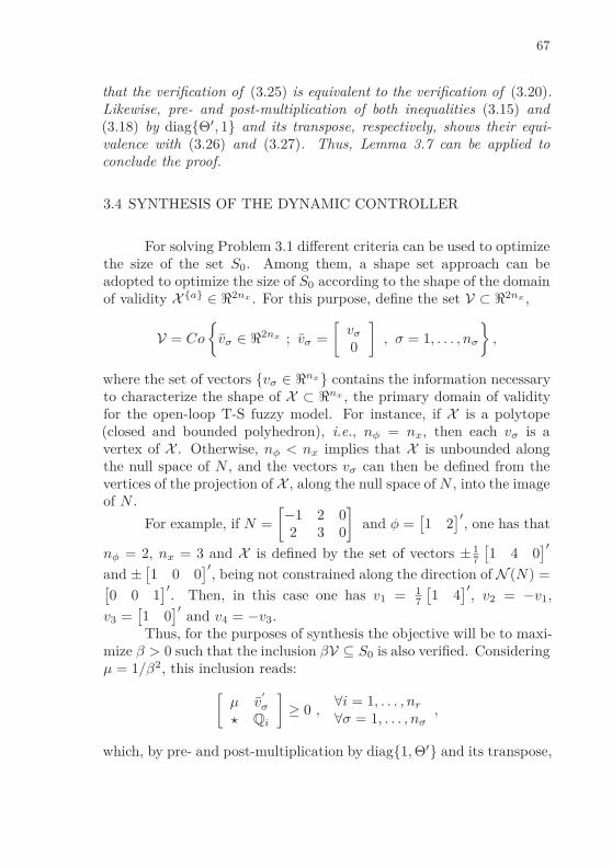
67
that the verification of (3.25) is equivalent to the verification of (3.20).Likewise, pre- and post-multiplication of both inequalities (3.15) and(3.18) by diagΘ′, 1 and its transpose, respectively, shows their equi-valence with (3.26) and (3.27). Thus, Lemma 3.7 can be applied toconclude the proof.
3.4 SYNTHESIS OF THE DYNAMIC CONTROLLER
For solving Problem 3.1 different criteria can be used to optimizethe size of the set S0. Among them, a shape set approach can beadopted to optimize the size of S0 according to the shape of the domainof validity X a ∈ ℜ2nx . For this purpose, define the set V ⊂ ℜ2nx ,
V = Co
vσ ∈ ℜ2nx ; vσ =
[
vσ
0
]
, σ = 1, . . . , nσ
,
where the set of vectors vσ ∈ ℜnx contains the information necessaryto characterize the shape of X ⊂ ℜnx , the primary domain of validityfor the open-loop T-S fuzzy model. For instance, if X is a polytope(closed and bounded polyhedron), i.e., nφ = nx, then each vσ is avertex of X . Otherwise, nφ < nx implies that X is unbounded alongthe null space of N , and the vectors vσ can then be defined from thevertices of the projection of X , along the null space of N , into the imageof N .
For example, if N =
[
−1 2 02 3 0
]
and φ =[
1 2]′
, one has that
nφ = 2, nx = 3 and X is defined by the set of vectors ± 17
[
1 4 0]′
and ±[
1 0 0]′
, being not constrained along the direction of N (N) =[
0 0 1]′
. Then, in this case one has v1 = 17
[
1 4]′
, v2 = −v1,
v3 =[
1 0]′
and v4 = −v3.Thus, for the purposes of synthesis the objective will be to maxi-
mize β > 0 such that the inclusion βV ⊆ S0 is also verified. Consideringµ = 1/β2, this inclusion reads:
[
µ v′
σ
⋆ Qi
]
≥ 0 ,∀i = 1, . . . , nr
∀σ = 1, . . . , nσ,
which, by pre- and post-multiplication by diag1, Θ′ and its transpose,
68
respectively, is equivalent to:
µ v′
σY v′
σ
⋆ Qi
≥ 0, i = 1, . . . , nr, σ = 1, . . . , nσ. (3.29)
In this way, by using Theorem 3.8 and condition (3.29), thefollowing convex optimization problem to synthesize the controller gainscan be proposed:
min
Q11i, Q12i, Q22i, Aij , Gij , X, Y, T, ∆, S,
Bij , Ci, Di, Ei, Fi, H11i, H12i, H2i
µ
subject to
LMIs (3.25), (3.26), (3.27) and (3.29).
(3.30)
3.5 EXPERIMENTS
3.5.1 Illustrative Example Continued
For this experiment it is considered the system of the IllustrativeExample 2.3 (see Chapter 2, section 2.3), now subject to amplitudebound control input
x(k + 1) = x3(k) + sin(x(k)) + (0.2 + x2(k))sat(u(k)) , y(k) = x(k)(3.31)
Although (3.31) represents a unidimensional system, its applica-tion here is interesting in terms of comparison and for graphical repre-sentation (the augmented space belongs to ℜ2).
Now, defining the sector nonlinearity ϕ(y(k)) = sin(y(k)) ∈S [0, 1], and considering the domain of validity defined by |x| ≤ 5π/12,it is obtained a N-Fuzzy model with two local nonlinear rules, with
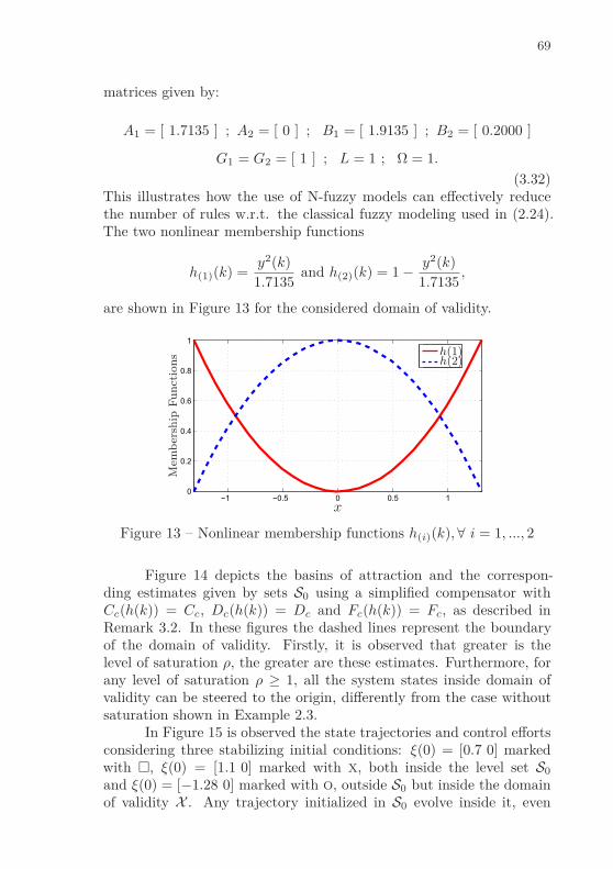
69
matrices given by:
A1 = [ 1.7135 ] ; A2 = [ 0 ] ; B1 = [ 1.9135 ] ; B2 = [ 0.2000 ]
G1 = G2 = [ 1 ] ; L = 1 ; Ω = 1.
(3.32)This illustrates how the use of N-fuzzy models can effectively reducethe number of rules w.r.t. the classical fuzzy modeling used in (2.24).The two nonlinear membership functions
h(1)(k) =y2(k)
1.7135and h(2)(k) = 1 − y2(k)
1.7135,
are shown in Figure 13 for the considered domain of validity.
−1 −0.5 0 0.5 10
0.2
0.4
0.6
0.8
1
x
Mem
ber
ship
Fu
nct
ion
s h(1)h(2)
Figure 13 – Nonlinear membership functions h(i)(k), ∀ i = 1, ..., 2
Figure 14 depicts the basins of attraction and the correspon-ding estimates given by sets S0 using a simplified compensator withCc(h(k)) = Cc, Dc(h(k)) = Dc and Fc(h(k)) = Fc, as described inRemark 3.2. In these figures the dashed lines represent the boundaryof the domain of validity. Firstly, it is observed that greater is thelevel of saturation ρ, the greater are these estimates. Furthermore, forany level of saturation ρ ≥ 1, all the system states inside domain ofvalidity can be steered to the origin, differently from the case withoutsaturation shown in Example 2.3.
In Figure 15 is observed the state trajectories and control effortsconsidering three stabilizing initial conditions: ξ(0) = [0.7 0] markedwith , ξ(0) = [1.1 0] marked with X, both inside the level set S0
and ξ(0) = [−1.28 0] marked with O, outside S0 but inside the domainof validity X . Any trajectory initialized in S0 evolve inside it, even
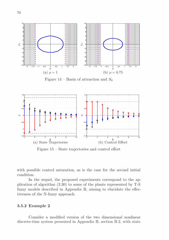
70
−2 −1.5 −1 −0.5 0 0.5 1 1.5 2−10
−8
−6
−4
−2
0
2
4
6
8
10
x
xc
(a) ρ = 1
−2 −1.5 −1 −0.5 0 0.5 1 1.5 2−10
−8
−6
−4
−2
0
2
4
6
8
10
x
xc
(b) ρ = 0.75
Figure 14 – Basin of attraction and S0
0 2 4 6 8 10−1.5
−1
−0.5
0
0.5
1
1.5
k
x
(a) State Trajectories
0 2 4 6 8 10−1.5
−1
−0.5
0
0.5
1
1.5
k
u
(b) Control Effort
Figure 15 – State trajectories and control effort
with possible control saturation, as is the case for the second initialcondition.
In the sequel, the proposed experiments correspond to the ap-plication of algorithm (3.30) to some of the plants represented by T-Sfuzzy models described in Appendix B, aiming to elucidate the effec-tiveness of the N-fuzzy approach.
3.5.2 Example 2
Consider a modified version of the two dimensional nonlineardiscrete-time system presented in Appendix B, section B.2, with state
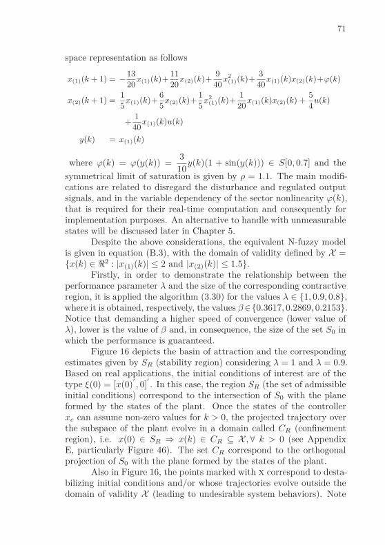
71
space representation as follows
x(1)(k + 1) = −13
20x(1)(k)+
11
20x(2)(k)+
9
40x
2(1)(k)+
3
40x(1)(k)x(2)(k)+ϕ(k)
x(2)(k + 1) =1
5x(1)(k)+
6
5x(2)(k)+
1
5x
2(1)(k)+
1
20x(1)(k)x(2)(k) +
5
4u(k)
+1
40x(1)(k)u(k)
y(k) = x(1)(k)
where ϕ(k) = ϕ(y(k)) =3
10y(k)(1 + sin(y(k))) ∈ S[0, 0.7] and the
symmetrical limit of saturation is given by ρ = 1.1. The main modifi-cations are related to disregard the disturbance and regulated outputsignals, and in the variable dependency of the sector nonlinearity ϕ(k),that is required for their real-time computation and consequently forimplementation purposes. An alternative to handle with unmeasurablestates will be discussed later in Chapter 5.
Despite the above considerations, the equivalent N-fuzzy modelis given in equation (B.3), with the domain of validity defined by X =x(k) ∈ ℜ2 : |x(1)(k)| ≤ 2 and |x(2)(k)| ≤ 1.5.
Firstly, in order to demonstrate the relationship between theperformance parameter λ and the size of the corresponding contractiveregion, it is applied the algorithm (3.30) for the values λ ∈ 1, 0.9, 0.8,where it is obtained, respectively, the values β ∈0.3617, 0.2869, 0.2153.Notice that demanding a higher speed of convergence (lower value ofλ), lower is the value of β and, in consequence, the size of the set S0 inwhich the performance is guaranteed.
Figure 16 depicts the basin of attraction and the correspondingestimates given by SR (stability region) considering λ = 1 and λ = 0.9.Based on real applications, the initial conditions of interest are of thetype ξ(0) = [x(0)
′
, 0]′
. In this case, the region SR (the set of admissibleinitial conditions) correspond to the intersection of S0 with the planeformed by the states of the plant. Once the states of the controllerxc can assume non-zero values for k > 0, the projected trajectory overthe subspace of the plant evolve in a domain called CR (confinementregion), i.e. x(0) ∈ SR ⇒ x(k) ∈ CR ⊆ X , ∀ k > 0 (see AppendixE, particularly Figure 46). The set CR correspond to the orthogonalprojection of S0 with the plane formed by the states of the plant.
Also in Figure 16, the points marked with X correspond to desta-bilizing initial conditions and/or whose trajectories evolve outside thedomain of validity X (leading to undesirable system behaviors). Note

72
−2 −1.5 −1 −0.5 0 0.5 1 1.5 2
−1.5
−1
−0.5
0
0.5
1
1.5
x(1)
x(2
)
XSRCRICs
(a) with λ = 1
−2 −1.5 −1 −0.5 0 0.5 1 1.5 2
−1.5
−1
−0.5
0
0.5
1
1.5
x(1)
x(2
)
XSRCRICs
(b) with λ = 0.9
Figure 16 – Basin of attraction and associated sets
that such a condition can exist even inside X , demonstrating againthe importance of considering the local characteristics of the T-S fuzzymodels. At last, comparing the sizes of SR it is possible to verify theaforementioned trade-off between λ and β.
For the temporal simulation is considered the initial condition
ξ(0) = [x(0)′
, 0]′
, with x(0) =[
1.15 1]
′
. This initial condition be-longs to the set of admissible initial conditions SR of the controllers de-signed with λ = 1 and λ = 0.9. As expected, the best time-performance,relative to the lower contractive parameter λ, can be observed compa-ring the state trajectories in Figure 17, as well as by comparison thedecrease of the Lyapunov function corresponding to these trajectories,as shown in Figure 18.
0 1 2 3 4 5 6 7 8 9 10−0.2
0
0.2
0.4
0.6
0.8
1
1.2
k
x1, x
2
(a) with λ = 1
0 1 2 3 4 5 6 7 8 9 10−0.2
0
0.2
0.4
0.6
0.8
1
1.2
k
x1, x
2
(b) with λ = 0.9
Figure 17 – State trajectories for example 1
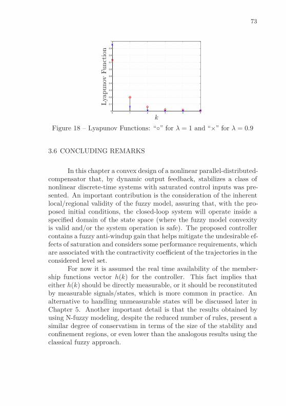
73
0 1 2 3 4 50
0.1
0.2
0.3
0.4
0.5
0.6
0.7
0.8
0.9
1
k
Lya
punov
Funct
ion
Figure 18 – Lyapunov Functions: “” for λ = 1 and “×” for λ = 0.9
3.6 CONCLUDING REMARKS
In this chapter a convex design of a nonlinear parallel-distributed-compensator that, by dynamic output feedback, stabilizes a class ofnonlinear discrete-time systems with saturated control inputs was pre-sented. An important contribution is the consideration of the inherentlocal/regional validity of the fuzzy model, assuring that, with the pro-posed initial conditions, the closed-loop system will operate inside aspecified domain of the state space (where the fuzzy model convexityis valid and/or the system operation is safe). The proposed controllercontains a fuzzy anti-windup gain that helps mitigate the undesirable ef-fects of saturation and considers some performance requirements, whichare associated with the contractivity coefficient of the trajectories in theconsidered level set.
For now it is assumed the real time availability of the member-ship functions vector h(k) for the controller. This fact implies thateither h(k) should be directly measurable, or it should be reconstitutedby measurable signals/states, which is more common in practice. Analternative to handling unmeasurable states will be discussed later inChapter 5. Another important detail is that the results obtained byusing N-fuzzy modeling, despite the reduced number of rules, present asimilar degree of conservatism in terms of the size of the stability andconfinement regions, or even lower than the analogous results using theclassical fuzzy approach.

74

4 CONTROL SYNTHESIS FOR NONLINEARSYSTEMS SUBJECT TO ENERGY BOUNDEDDISTURBANCES
In this chapter, it is addressed the local stabilization problem ofnonlinear discrete-time systems subject to energy bounded disturbancesby means of T-S fuzzy models. The proposed controller consists ofa nonlinear state feedback which depends on the fuzzy membershipfunction as well as the sector bounded nonlinearities, in the case of an N-fuzzy model. In this setup, LMI control design conditions are proposedto locally ensure the input-to-state stability in the ℓ2-sense (ℓ2-ISS)and a certain input-to-output performance (i.e., an upper bound forthe system ℓ2-gain) of the original nonlinear discrete-time system.
Additionally, the design conditions provide an estimate of theclosed-loop reachable set (that is, a region inside the T-S domain of va-lidity which bounds the state trajectories driven by the admissible classof ℓ2 disturbances). Finally, three (convex) optimization problems areproposed to either minimize the estimate of the reachable set, improvethe disturbance tolerance or minimize the ℓ2-gain from the disturbanceinput to the regulated output; and numerical examples are consideredto demonstrate the effectiveness of the proposed approach as a con-trol design tool for nonlinear discrete-time systems subject to energybounded disturbances. The results presented here are based on theworks Klug, Castelan & Coutinho (2013), in which the ISS in the ℓ2-sense was first investigated, and Klug, Castelan & Coutinho (2015b).
4.1 PROBLEM FORMULATION
Consider the class of nonlinear systems in (2.1) with the additionof a regulated output vector zk ∈ Z ⊂ ℜnz , represented by
x(k + 1) = f(x(k)) + V (x(k))u(k) + T (x(k))w(k)z(k) = fz(x(k)) + Vz(x(k))u(k) + Tz(x(k))w(k)
(4.1)
where x(k) ∈ X ⊂ ℜnx , u(k) ∈ U ⊂ ℜnu and wk ∈ W ⊂ ℜnw arerespectively the state, the control input and the exogenous disturbancevectors. The functions f(·) : ℜnx −→ ℜnx , with f(0) = 0, fz(·) :ℜnx −→ ℜnz , with fz(0) = 0, V (·) : ℜnx −→ ℜnx×nu , Vz(·) : ℜnx −→ℜnz×nu , T (·) : ℜnx −→ ℜnx×nw and Tz(·) : ℜnx −→ ℜnz×nw arecontinuous and bounded for all x(k) ∈ X . The additional signal z(k)is required for the desired control purposes.

76
In order to design a state feedback control law uk = κ(xk), thenonlinear system (4.1) will be represented by means of N-fuzzy model(using the procedure explained in section 2.2 with similar steps for thenonlinearities in the vector z(k)), described through the defuzzificationmethod by center of gravity as
x(k + 1)=A(h(k))x(k)+B(h(k))u(k)+Bw(h(k))w(k)+G(h(k))ϕ(k)z(k)=Cz(h(k))x(k)+Bz(h(k))u(k)+Bzw(h(k))w(k)+Gz(h(k))ϕ(k)
(4.2)The disturbance input vector w(k) is assumed to lie inside the followingclass of square summable sequences:
W := w(k) : ‖w(k)‖2ℓ2
≤ δ−1, (4.3)
where δ is a positive scalar defining the size of W (i.e., the energy boundof w(k)). The set W will be often referred as the class of admissibledisturbances.
Complementing the fuzzy model description (4.2), the vector ofnonlinearities ϕ(k) = ϕ(Lx(k)) ∈ ℜnϕ verifies (at least locally) thesector condition (2.3), and the matrix structure is given by:
[
A(h(k)) B(h(k)) Bw(h(k)) G(h(k))Cz(h(k)) Bz(h(k)) Bzw(h(k)) Gz(h(k))
]
=
nr∑
i=1
h(i)(k)
[
Ai Bi Bwi Gi
Czi Bzi Bzwi Gzi
]
.
At last, the T-S model domain of validity X is described by (2.17). Itshould be remembered that x(k) ∈ X ⇒ h(k) ∈ Ξ, with Ξ as defined in(3.2), i.e. X is a region of the state space where the convexity propertyof set (3.2) holds true. Such domain of validity must be taken intoaccount by any control synthesis or stability analysis condition thatassumes description (4.2) instead of (4.1). In particular, loss of per-formance or even instability may occur when state trajectories evolveoutside the domain of validity of the model (4.2). In this sense, onepurpose is to handle the domain of validity of the T-S model into thecontroller synthesis stage to assure local closed-loop stability.
Assuming that the normalized membership functions h(k) canbe computed in real-time, a nonlinear controller can be proposed withthe same fuzzy rules as the nonlinear T-S model in (4.2). In this case,the following nonlinear state feedback control law is proposed:
77
u(k) = κ(xk) = K(h(k))x(k) + Γ(h(k))ϕ(k) (4.4)
where[
K(h(k)) Γ(h(k))]
=nr∑
i=1
h(i)(k)[
Ki Γi
]
, with Ki ∈ ℜnu×nx
and Γi ∈ ℜnu×nϕ .Taking (4.2) and (4.4) into account, the closed-loop T-S fuzzy
model is as follows:
x(k + 1) = A(h(k))x(k) + Bw(h(k))w(k) + G(h(k))ϕ(k)z(k) = C(h(k))x(k) + Bzw(h(k))w(k) + F(h(k))ϕ(k)
(4.5)
withA(h(k)) = A(h(k)) + B(h(k))K(h(k)),G(h(k)) = G(h(k)) + B(h(k))Γ(h(k)),C(h(k)) = Cz(h(k)) + Bz(h(k))K(h(k)) andF(h(k)) = Gz(h(k)) + Bz(h(k))Γ(h(k)).
The closed-loop matrices A(h(k)), G(h(k)), C(h(k)) and F(h(k)) canbe generically rewritten, through summation properties, as
T (h(k)) =nr∑
i=1
nr∑
j=i
(1 + ςij)h(i)(k)h(j)(k)Ti + XiYj + Tj + XjYi
2(4.6)
where the tuple (T , T, X, Y ) represents either (A, A, B, K), (G, G, B, Γ),(C, Cz, Bz, K) or (F , Gz, Bz, Γ), and ςij is a binary variable such that(as previously defined in (3.8))
ςij =
1 if i 6= j,0 otherwise.
(4.7)
Notice that the ℓ2-ISS of system (4.5) for all h(k) ∈ Ξ impliesthat the original nonlinear system in (4.1) with (4.4) is also ISS stable.This is satisfied if the trajectory x(k) of (4.5) driven by w(k) ∈ Wremains in X for all k ≥ 0. In order to obtain LMI constraints guaran-teeing the state trajectory boundness inside X , the following problemwill be addressed in this work.
Problem 4.1 Determine the gain matrices Ki and Γi, for i = 1, ..., nr,such that the trajectories of system (4.5) remain bounded in some re-gion D containing the origin such that D ⊂ X for any w(k) ∈ W andfor all h(k) ∈ Ξ. In addition, determine a positive constant γ whichbounds the induced ℓ2-norm from w(k) to z(k).

78
From the above control problem different optimization designcriteria can be considered to compute the matrices Ki and Γi, as forexample to minimize the ℓ2-gain (by minimizing γ), to maximize thesize of the class of admissible disturbances (by minimizing δ) or tominimize the size of a trajectory bounding set for a given class of ad-missible disturbances W (by considering that δ and γ are given). Theseoptimization problems are better discussed later.
To end this section, some preliminary results which will be in-strumental to derive the synthesis conditions are given below.
Let V (x(k), h(k)) be a fuzzy Lyapunov function (FLF)
V (x(k), h(k)) : ℜnx × Ξ → ℜ+ , V (0, h(k)) = 0∀ h(k) ∈ Ξ (4.8)
and the set D defined as follows
D = x(k) ∈ ℜnx : V (x(k), h(k)) ≤ δ−1, ∀ h(k) ∈ Ξ , (4.9)
where δ is the positive scalar defining the bound of W in (4.3).In the following, it is defined the notion of input-to-state stability
in the ℓ2-sense for nonlinear discrete-time systems to be considered inthis thesis.
Definition 4.2 Consider the system (4.1), with x(0) = 0, and thelevel set D as defined in (4.9) for a given positive scalar δ. The unforcedsystem in (4.1) is said to be ℓ2-ISSD (input-to-state stable with respectto D), if for any w(k) ∈ W the system state x(k) remains bounded inD for all k ≥ 0.
Observe that the above definition implies that D is a positivelyinvariant set. Thus, x(0) ∈ D implies that
V (x(k), h(k)) ≤ δ−1 , ∀ k ≥ 0 , h(k) ∈ Ξ . (4.10)
Lemma 4.3 The unforced system (4.1), with x(0) = 0, is ℓ2-ISSD
and there exists an upper bound γ on the ℓ2-gain from w(k) to z(k) ifthe following holds for all x(k) ∈ D, h(k) ∈ Ξ and w(k) ∈ W:
∆V (k)= V (x(k + 1), h(k + 1)) − V (x(k), h(k))
+ γ−2z′
(k)z(k) − w′
(k)w(k) < 0 (4.11)
Proof Assume that (4.11) holds ∀ x(k) ∈ D, h(k) ∈ Ξ, w(k) ∈ W.
79
Then, for any k > 0, leads to:
k−1∑
k=0
∆V (k) = V(
x(k), h(k))
− V (x(0), h(0))
+γ−2
k−1∑
k=0
z(k)′
z(k) −k−1∑
k=0
w(k)′
w(k) < 0
(4.12)
Thus, in view of (4.3) and (4.8), the above implies:
i) ℓ2 input-to-state stability: note that V (x(0), h(0)) = 0, since x(0) =0. Then, it has V
(
x(k), h(k))
≤ ‖w(k)‖22 ≤ δ−1, ∀ k > 0. That is,
D is a positive invariant set.
ii) input-to-output performance: taking k → ∞, it follows that ‖z(k)‖2 <γ‖w(k)‖2. That is, γ is an upper-bound on the system ℓ2-gain.
iii) internal stability: let k be a positive integer. If w(k) = 0 for allk ≥ k, then the condition in (4.11) implies that V (x(k + 1), h(k +1))−V (x(k), h(k)) < −γ−2z(k)
′
z(k) < 0 guaranteeing that x(k) →0 as k → ∞. In other words, D is a contractive positive invari-ant set whenever the disturbance w(k) vanishes (see, e.g., (KLUG;
CASTELAN; LEITE, 2011)).
4.2 CONTROL DESIGN
For the purpose of synthesizing the controller (4.4) which ensuresthat the nonlinear system (4.1) is locally ℓ2-ISSD in closed-loop, it isconsidered the N-Fuzzy representation given in (4.5). To this end, letthe following FLF:
V (x(k), h(k)) = x(k)′
Q−1(h(k))x(k), Q(h(k)) =nr∑
i=1
hk(i)Qi , (4.13)
with Qi = Q′
i > 0 ∈ ℜnx×nx , i=1, . . . , nr, to be determined.In light of the above, it is required to consider D ⊂ X for all
h(k) ∈ Ξ in Lemma 4.3 to guarantee the convexity of the fuzzy modelin (4.5). Furthermore, it can be shown that the level set D as definedin (4.9) with (4.13) will be the intersection of nr ellipsoidal sets (HU; Z.;
M., 2002; JUNGERS; CASTELAN, 2011), given by
D =
⋂
i∈1,...nr
E(Q−1i , δ−1) (4.14)
80
where E(Q−1i , δ−1) =
x(k) ∈ ℜnx : x(k)′
Q−1i x(k) ≤ δ−1
is the i-th
ellipsoidal set.In the sequel, sufficient design conditions based on LMIs to deter-
mine the control law (4.4) which locally stabilizes the nonlinear system(4.1) in the ℓ2-ISSD sense are presented.
Theorem 4.4 Suppose there exist symmetric positive definite matri-ces Qi ∈ ℜnx×nx , i = 1, . . . , nr; a diagonal positive definite matrix∆ ∈ ℜnϕ×nϕ ; matrices Y1i ∈ ℜnu×nx , Y2i ∈ ℜnu×nϕ , i = 1, . . . , nr,and U ∈ ℜnx×nx ; and positive scalars δ and γ satisfying the followingLMIs:
−Qq Π1ij Π3
ij
Bwi + Bwj
20
⋆ Π2ij U
′
L′
Ω 0 Π4ij
⋆ ⋆ −2∆ 0 Π5ij
⋆ ⋆ ⋆ −γ2IB
′
zwi + B′
zwj
2⋆ ⋆ ⋆ ⋆ −I
< 0
∀ q, i = 1, . . . , nr and j = i, . . . , nr
(4.15)
[
−Qi QiN′
ℓ
⋆ −δφ2ℓ
]
≤ 0 , ∀ i = 1, . . . , nr and ℓ = 1, . . . , nφ , (4.16)
where
Π1ij = 0.5 (AiU + BiY1j + AjU + BjY1i) ,
Π2ij = 0.5 (Qi + Qj) − U − U
′
,
Π3ij = 0.5 (Gi∆ + BiY2j + Gj∆ + BjY2i) ,
Π4ij = 0.5
(
U′
C′
zi + Y′
1iB′
zj + U′
Czj + Y′
1jB′
zi
)
,
Π5ij = 0.5
(
∆G′
zi + Y′
2iB′
zj + ∆G′
zj + Y′
2jB′
zi
)
.
(4.17)
Let Ki = Y1iU−1 and Γi = Y2i∆−1, i = 1, . . . , nr. In addition,
consider the nonlinear system (4.1), with (4.4), and its exact N-fuzzyrepresentation in (4.5). Then, the following holds for zero initial con-ditions:
a) x(k) remains bounded in D for any w(k) ∈ W;
b) ‖z(k)‖2 ≤ γ ‖w(k)‖2 for all w(k) ∈ W;
c) x(k) → 0 as k → ∞ if there exists k > 0 such that w(k) = 0 forall k ≥ k;

81
d) D ⊆ E(Q−1i , δ−1) ⊂ X , for i = 1, ..., nr.
Proof Assume that (4.15) is verified for all q, i = 1, . . . , nr and j =i, . . . , nr. Replace Y1i and Y2i respectively by KiU and Γi∆. Multiplythe resulting inequalities successively by h(i)(k), h(j)(k), h(q)(k + 1),and sum up on i, q = 1, . . . , nr and j = i, . . . , nr. Thus, the inequalityM(h(k)) < 0 holds if h(k) ∈ Ξ with
M(h) =
−Q(h+) A(h)U G(h)∆ Bw(h) 0⋆ U ′Q−1(h)U U ′L
′
Ω 0 U′C(h)
⋆ ⋆ −2∆ 0 ∆F(h)⋆ ⋆ ⋆ −γ2I B
′
zw(h)⋆ ⋆ ⋆ ⋆ −I
and the shorthands h = h(k) and h+ = h(k+1). Note that the matricesQ(h), Bw(h) and Bzw(h) can be written as (SILVA et al., 2014)
Q(h)Bw(h)Bzw(h)
=nr∑
i=1
nr∑
j=i
(1 + ςij)h(i)(k)h(j)(k)
1
2
Qi + Qj
Bwi + Bwj
Bzwi + Bzwj
,
and that U ′Q−1(h)U ≥ −Q(h) + U ′ + U is verified since U is full rankfrom the (2, 2) block of the left-hand side of (4.15).
Further, let the congruence transformation ΠM(h)Π′
with
Π =
0 I 0 0 00 0 0 (U
′
)−1 00 0 ∆−1 0 0I 0 0 0 00 0 0 0 I
.
Thus, applying the Schur’s complement to ΠM(h)Π′
< 0 yields:
MS(h) = ϑ′
1(k)Q−1(h+)ϑ1(k) +
C′
(h)B
′
zw(h)F ′
(h)
C′
(h)B
′
zw(h)F ′
(h)
′
−
Q−1(h) 0 −L′
Ω∆−1
0 γ2I 0−∆−1ΩL 0 2∆−1
< 0 . (4.18)
with ϑ1(k) =[
A(h(k)) Bw(h(k)) G(h(k))]
.
82
Now, let ϑ2(k) =[
x′
(k) w′
(k) ϕ′
(k)]′
. Then, in view of (4.18), onehas that:
ϑ′
2(k)MS(h(k))ϑ2(k) = ∆V (k) − 2ϕ′
(k)∆−1(ϕ(k) − ΩLx(k)) < 0 ,(4.19)
if h(k) ∈ Ξ.Hence, the condition (4.19) implies that ∆V (k) < 0 whenever
h(k) ∈ Ξ and the sector condition (2.3) is verified. Assuming that x(k)does not leave X , for all k ≥ 0, it is inferred that condition (4.12) isalso satisfied. In this way the properties a), b) and c) in Theorem 4.4are guaranteed, and consequently i), ii) and iii) from Lemma 4.3.
Now, it is required to show that x(k) ∈ X , for all k ≥ 0, andconsequently h(k) ∈ Ξ. To this end, assume that (4.16) is verified.Then, multiplying (4.16) by h(i)(k) and summing up on i = 1, . . . , nr
leads to:
Λ =
[
−Q(h(k)) Q(h(k))N′
ℓ
⋆ −δφ2ℓ
]
≤ 0.
Let F = diagQ−1(h(k)), 1. Hence, the congruence transformationF ′
ΛF = Λ yields
Λ =
[
−Q−1(h(k)) N′
ℓ
⋆ −δφ2ℓ
]
≤ 0.
By applying the Schur’s complement to Λ, it is obtained:
N′
ℓ(δφ2ℓ)−1Nℓ − Q−1(h(k)) ≤ 0.
Pre- and post-multiplying the above respectively by x(k)′
and x(k) andconsidering the S-procedure leads to:
x′
(k)N′
ℓφ−2ℓNℓx(k) ≤ 1, ∀ x(k) ∈ D ,
D = x : x′
(k)Q−1(h(k))x(k) ≤ δ−1That is, E(Q−1
i , δ−1) ⊂ X , ∀i = 1, ..., nr. Recalling from (4.14) thatD ⊆ E(Q−1
i , δ−1), it is possible to ensure the property d) and inferfrom Lemma 4.3 that x(k) ∈ D, for all k ≥ 0, which concludes theproof.
Remark 4.5 It is possible to apply Theorem 4.4 to systems repre-sented by classical T-S fuzzy models (without the nonlinear term) by

83
eliminating the third row and column block of the matrix on the left-hand side of (4.15).
Remark 4.6 It is interesting to note that the stabilization condition(4.15) has a reduced number of LMIs when compared to other tech-niques in literature. This is due to the use of the property (4.6) and thedefinition of the variable ςij in (4.7). See, for instance, Theorem 6.6of (FENG, 2010), where the resulting LMIs are required to be verified∀ i, j, q = 1, ..., nr.
4.3 DESIGN ISSUES
Now, three extensions of Theorem 4.4 are proposed. The pur-pose is to demonstrate the potential of the described approach as a con-trol design tool for nonlinear discrete-time systems subject to energybounded disturbances.
4.3.1 Disturbance Tolerance
The disturbance tolerance criterion consists in maximizing abound on the disturbance energy to which one can ensure that the sys-tem trajectories remain bounded (and inside the domain of validity).This can be accomplished by the following optimization problem.
min δQi, ∆, Y1i, Y2i, U
subject toLMIs (4.15) and (4.16).
(4.20)
Notice that the minimization of δ implies in maximizing the setof admissible disturbances W.
4.3.2 Disturbance Attenuation
For a given disturbance energy level δ−1, the disturbance atte-nuation criterion consists in minimizing an upper bound on the ℓ2-gainfrom w(k) to z(k) while guaranteeing that x(k) ∈ X , which can beobtained from the solution of the following optimization problem:
min γQi, ∆, Y1i, Y2i, U
subject toLMIs (4.15) and (4.16).
(4.21)
84
4.3.3 Reachable Set Estimation
The reachable set estimation criterion consists in minimizing theset D (an estimate of the reachable set) for a specific disturbance energylevel δ−1 and a guaranteed bound γ on the system ℓ2-gain. This objec-tive can be accomplished by considering the inclusion E(Q−1
i , δ−1) ⊂βX , ∀i = 1, ..., nr, β ∈ (0, 1], which is obtained by modifying the con-dition in (4.16) as follows:
[
−Qi QiN′
ℓ
⋆ −β2δφ2ℓ
]
≤ 0
∀i = 1, ..., nr and ℓ = 1, ..., η
(4.22)
Then, the objective is to obtain the lowest value for β which willbe useful in practice whenever the effects of the disturbances over thesystem trajectories are to be minimized. This criteria can be obtainedby the following optimization problem:
min βQi, ∆, Y1i, Y2i, U
subject toLMIs (4.15), (4.22) and 0 < β ≤ 1 .
(4.23)
4.4 EXPERIMENTS
Two numerical examples are presented in this section. The firstone demonstrates some stability issues that can occur when the domainof validity is not considered. In this sense a nonlinear plant is modeledby the classical T-S form and the region X , where the model conve-xity is guaranteed, is not taken into account in the design phase. Inthe second example, it is shown the effectiveness of the proposed tech-nique considering the optimization problems described in the previoussection.
4.4.1 Example 1
Consider the control problem of backing-up a truck-trailer asstudied in Lo & Lin (2003). The state space representation of the
85
system is described by (see Appendix B)
x(1)(k + 1) = x(1)(k) − vT
L sin(x(1)(k)) +vT
lu(k)
x(2)(k + 1) = x(2)(k) +vT
L sin(x(1)(k)) + 0.2w(k)
x(3)(k + 1) = x(3)(k) + vT cos(x(1)(k)) sin(x(2)(k)
+vT
2L sin(x(1)(k))) + 0.1w(k)
z(k) = 7x(1)(k) − vTx(2)(k) + 0.03x(3)(k) − vT
lu(k)
where the variables definitions, constant values, and their equivalentfuzzy representation are presented in section B.3, equation (B.5), withX = x(k) ∈ ℜ2 : |x(1)(k)| ≤ π/3 and |x(2)(k)| ≤ 170π/180. Inorder to allow a comparison with other techniques was considered theclassical modeling, resulting in eight linear local rules for the model.The objective is to demonstrate the problems that can occur in practicewhen the model validity domain is not considered (usually assumed inthe literature).
In light of the above, and for comparison purposes, the followingcontrol approaches using classical T-S fuzzy models are taken into ac-count:
• case 1 - Theorem 6.6 of (FENG, 2010);
• case 2 - Remark 4.5 without the inclusion constraint in (4.16).
By solving an optimization problem aiming the minimization of the up-per bound on the ℓ2-gain from w(k) to z(k), it is respectively obtainedthe upper-bounds γ = 0.4171 and γ = 0.3430 for the cases 1 and 2.Notice that the bound obtained in case 2 is less conservative than theone obtained in case 1.
Figure 19 shows the projections of the closed-loop system trajec-tories1 on the plane x(1), x(2) and ℓ2-gains using the results obtainedin case 1, for the following three different disturbance signals with‖w1(k)‖ℓ2
= 7.8731, ‖w2(k)‖ℓ2= 10.3923 and ‖w3(k)‖ℓ2
= 24,
w1(k) =
ek, 1 ≤ k ≤ 20, k < 1, k > 2
, w2(k) =
−6, 1 ≤ k ≤ 30, k < 1, k > 3
,
1The simulations were performed considering the closed-loop system composedof the designed fuzzy controller and the original nonlinear plant
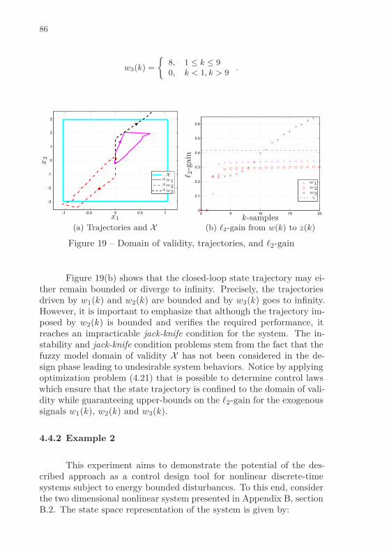
86
w3(k) =
8, 1 ≤ k ≤ 90, k < 1, k > 9
.
-1 -0.5 0 0.5 1
-3
-2
-1
0
1
2
3
x1
x2
Xxw1xw2xw3
(a) Trajectories and X
0 5 10 15 200
0.1
0.2
0.3
0.4
0.5
0.6
k-samples
ℓ 2-g
ain
w1w2w3γ
(b) ℓ2-gain from w(k) to z(k)
Figure 19 – Domain of validity, trajectories, and ℓ2-gain
Figure 19(b) shows that the closed-loop state trajectory may ei-ther remain bounded or diverge to infinity. Precisely, the trajectoriesdriven by w1(k) and w2(k) are bounded and by w3(k) goes to infinity.However, it is important to emphasize that although the trajectory im-posed by w2(k) is bounded and verifies the required performance, itreaches an impracticable jack-knife condition for the system. The in-stability and jack-knife condition problems stem from the fact that thefuzzy model domain of validity X has not been considered in the de-sign phase leading to undesirable system behaviors. Notice by applyingoptimization problem (4.21) that is possible to determine control lawswhich ensure that the state trajectory is confined to the domain of vali-dity while guaranteeing upper-bounds on the ℓ2-gain for the exogenoussignals w1(k), w2(k) and w3(k).
4.4.2 Example 2
This experiment aims to demonstrate the potential of the des-cribed approach as a control design tool for nonlinear discrete-timesystems subject to energy bounded disturbances. To this end, considerthe two dimensional nonlinear system presented in Appendix B, sectionB.2. The state space representation of the system is given by:
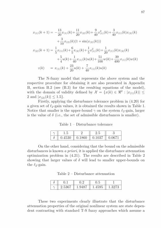
87
x(1)(k + 1) = −13
20x(1)(k)+
11
20x(2)(k)+
9
40x
2(1)(k)+
3
40x(1)(k)x(2)(k)
+3
10x(2)(k)(1 + sin(x(2)(k)))
x(2)(k + 1) =1
5x(1)(k)+
6
5x(2)(k)+
1
5x
2(1)(k)+
1
20x(1)(k)x(2)(k)
+5
4u(k)+
1
40x(1)(k)u(k)+
51
100w(k)+
39
400x(1)(k)w(k)
z(k) = x(1)(k) +23
20u(k) +
7
40x(1)(k)u(k)
The N-fuzzy model that represents the above system and therespective procedure for obtaining it are also presented in AppendixB, section B.2 (see (B.3) for the resulting equations of the model),with the domain of validity defined by X = x(k) ∈ ℜ2 : |x(1)(k)| ≤2 and |x(2)(k)| ≤ 1.5.
Firstly, applying the disturbance tolerance problem in (4.20) fora given set of ℓ2-gain values, it is obtained the results shown in Table 1.Notice that smaller is the upper-bound γ on the system ℓ2-gain, largeris the value of δ (i.e., the set of admissible disturbances is smaller).
Table 1 – Disturbance tolerance
γ 1.5 2 2.5 3δ 0.4530 0.1860 0.1037 0.0671
On the other hand, considering that the bound on the admissibledisturbances is known a priori, it is applied the disturbance attenuationoptimization problem in (4.21). The results are described in Table 2showing that larger values of δ will lead to smaller upper-bounds onthe ℓ2-gain.
Table 2 – Disturbance attenuation
δ 0.1 0.2 0.5 1γ 2.5367 1.9487 1.4595 1.3273
These two experiments clearly illustrate that the disturbanceattenuation properties of the original nonlinear system are state depen-dent contrasting with standard T-S fuzzy approaches which assume a
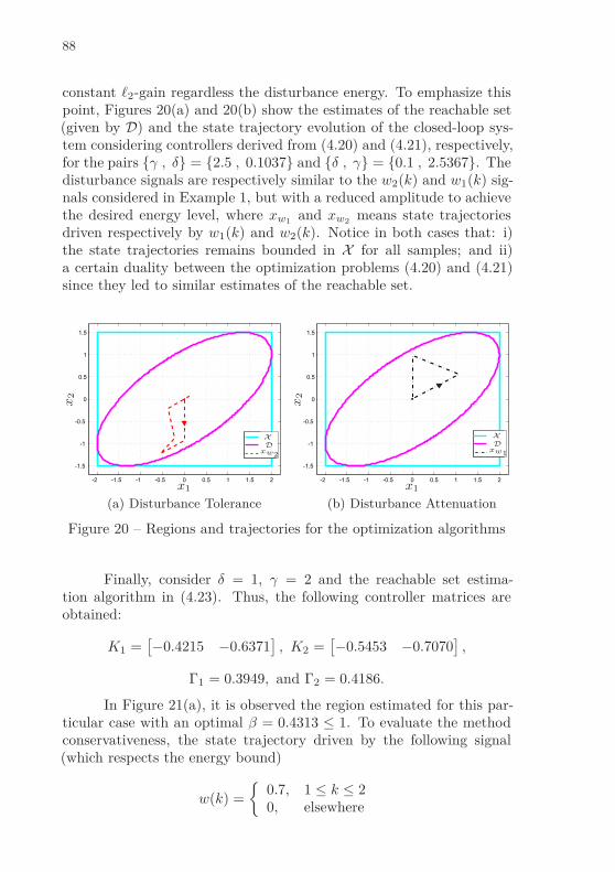
88
constant ℓ2-gain regardless the disturbance energy. To emphasize thispoint, Figures 20(a) and 20(b) show the estimates of the reachable set(given by D) and the state trajectory evolution of the closed-loop sys-tem considering controllers derived from (4.20) and (4.21), respectively,for the pairs γ , δ = 2.5 , 0.1037 and δ , γ = 0.1 , 2.5367. Thedisturbance signals are respectively similar to the w2(k) and w1(k) sig-nals considered in Example 1, but with a reduced amplitude to achievethe desired energy level, where xw1
and xw2means state trajectories
driven respectively by w1(k) and w2(k). Notice in both cases that: i)the state trajectories remains bounded in X for all samples; and ii)a certain duality between the optimization problems (4.20) and (4.21)since they led to similar estimates of the reachable set.
-2 -1.5 -1 -0.5 0 0.5 1 1.5 2
-1.5
-1
-0.5
0
0.5
1
1.5
x1
x2
X
Dxw2
(a) Disturbance Tolerance
-2 -1.5 -1 -0.5 0 0.5 1 1.5 2
-1.5
-1
-0.5
0
0.5
1
1.5
x1
x2
X
Dxw1
(b) Disturbance Attenuation
Figure 20 – Regions and trajectories for the optimization algorithms
Finally, consider δ = 1, γ = 2 and the reachable set estima-tion algorithm in (4.23). Thus, the following controller matrices areobtained:
K1 =[
−0.4215 −0.6371]
, K2 =[
−0.5453 −0.7070]
,
Γ1 = 0.3949, and Γ2 = 0.4186.
In Figure 21(a), it is observed the region estimated for this par-ticular case with an optimal β = 0.4313 ≤ 1. To evaluate the methodconservativeness, the state trajectory driven by the following signal(which respects the energy bound)
w(k) =
0.7, 1 ≤ k ≤ 20, elsewhere

89
is also plotted in Figure 21(a), demonstrating that the reachable setestimate is tight. For illustrative purposes, the time response of thestate trajectories and the control effort are shown in Figures 21(b) and22, respectively.
-2 -1.5 -1 -0.5 0 0.5 1 1.5 2
-1.5
-1
-0.5
0
0.5
1
1.5
x1
x2
X
βX
Dxw
(a) Reachable Set Estimation
0 1 2 3 4 5 6-0.1
0
0.1
0.2
0.3
0.4
0.5
0.6
k-th samplest
ate
s
x1x2
(b) State trajectories
Figure 21 – Regions and trajectories
0 1 2 3 4 5 6-0.5
-0.4
-0.3
-0.2
-0.1
0
0.1
k-th sample
uk
Figure 22 – Control effort
4.5 CONCLUDING REMARKS
A convex approach for the design of fuzzy controllers that locallystabilizes nonlinear discrete-time systems subject to energy boundeddisturbances was addressed in this chapter. Considering fuzzy Lya-punov functions, three optimization problems in terms of LMI cons-traints were proposed to design a nonlinear state-feedback control law,

90
which is a function of the membership fuzzy functions and cone sec-tor nonlinearities. It turns out that the provided approach locally en-sures the ℓ2-ISS of the original nonlinear system while guaranteeing acertain input-to-output performance for a given class of disturbancesignals. Also, the numerical examples stressed this ability of the pro-posed methodology to deal with the ℓ2-control problems in a morerealistic basis than other existing fuzzy techniques that do not considerthe regional validity problematic. Additionally, it is worth mentioningthat the considered problem can be extended to deal with the localℓ2-ISS stabilization problem in the presence of control saturation (TAR-
BOURIECH et al., 2011a), using the framework described in the previouschapter.

5 CONTROL SYNTHESIS FOR NONLINEARSYSTEMS SUBJECT TO AMPLITUDE BOUNDEDDISTURBANCES
In this chapter the local stabilization problem of nonlinear discre-te-time systems subject to amplitude bounded disturbances is addressedby means of T-S fuzzy models. Note that even though the dynamicsof exogenous persistent signals are generally unknown, it is commonto obtain an upper and a lower bound of the values that the signalcan assume over time. It is also worth noting that in the presence ofamplitude bounded disturbances, the asymptotic stability of the origincan not be guaranteed and in this case the concept of ultimate bounded(UB) stability is considered (i.e., the state trajectory is guaranteed toconverge to a region in the vicinity of the system origin).
The proposed controllers are based on the state and dynamicoutput feedback, and the main contribution is related to the use oftwo ellipsoidal sets, EE and EI , both contained in the region of validityof the fuzzy model, which have different shapes and are respectivelyassociated with the set of admissible initial conditions and the conceptof UB stability. In other words, the state trajectories starting in theset EE will converge in finite-time to the internal set EI and never leaveit. In addition, the design conditions ensure that the state trajectorydriven by admissible (amplitude bounded) disturbances remains insidethe T-S domain of validity guaranteeing the closed-loop UB stability ofthe original nonlinear system. An optimization problem is proposed tomaximize EE and to minimize EI . The results presented here are basedon the work Klug, Castelan & Coutinho (2015).
5.1 PROBLEM FORMULATION
Consider the class of nonlinear systems with state space repre-sentation affine in the input and disturbance signals defined in Chapter2, which equation (2.1) is repeated here for sake of completeness:
x(k + 1) = f(x(k)) + V (x(k))u(k) + T (x(k))w(k)y(k) = Cx(k)
where x(k) ∈ X ⊂ ℜnx , u(k) ∈ U ⊂ ℜnu , y(k) ∈ Y ⊂ ℜny are respec-tively the state, the control input and the system output vectors. Thefunctions f(·) : ℜnx −→ ℜnx , with f(0) = 0, V (·) : ℜnx −→ ℜnx×nu
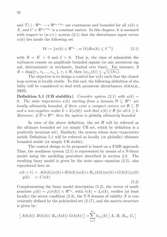
92
and T (·) : ℜnx −→ ℜnx×nw are continuous and bounded for all x(k) ∈X , and C ∈ ℜny×nx is a constant matrix. In this chapter, it is assumedwith respect to (w.r.t.) system (2.1) that the disturbance input vectorw(k) lies inside the following set:
W := w(k) ∈ ℜnw : w′
(k)Rw(k) ≤ δ−1 (5.1)
with R = R′
> 0 and δ > 0. That is, the class of admissible dis-turbances consist on amplitude bounded signals (or any persistent sig-nal, deterministic or stochastic, limited over time). For instance, ifR = diagr1, r2, ..., rnw
, ri ∈ ℜ, then∣
∣w(i)(k)∣
∣ ≤√
1/(δri).The objective is to design a control law u(k) such that the closed-
loop system is locally stable. To this end, the following definition of sta-bility will be considered to deal with persistent disturbances (KHALIL,2003).
Definition 5.1 (UB stability) Consider system (2.1) with u(k) =0. The state trajectories x(k) starting from a domain D ⊆ ℜnx arelocally ultimately bounded, if there exist a compact convex set B ⊆ Dand a non-negative scalar k = k(x(0)) such that x(k) ∈ B for all k ≥ k.Moreover, if D ≡ ℜnx then the system is globally ultimately bounded.
In view of the above definition, the set B will be referred asthe ultimate bounded set (or simply UB set, which by definition is apositively invariant set). Similarly, the system whose state trajectoriessatisfy Definition 5.1 will be referred as locally (or globally) ultimatebounded stable (or simply UB stable).
The control design to be proposed is based on a FMB approach.Thus, the nonlinear system (2.1) is represented by means of a N-fuzzymodel using the modeling procedure described in section 2.2. Theresulting fuzzy model is given by the state space equation (2.5), alsoreproduced here as
x(k + 1) = A(h(k))x(k)+B(h(k))u(k)+Bw(h(k))w(k)+G(h(k))ϕ(k)y(k) = Cx(k)
(5.2)Complementing the fuzzy model description (5.2), the vector of nonli-nearities ϕ(k) = ϕ(π(k)) ∈ ℜnϕ , with π(k) = Lx(k), verifies (at leastlocally) the sector condition (2.3), the T-S domain of validity X is con-veniently defined by the polyhedral set (2.17), and the matrix structureis given by:
[
A(h(k)) B(h(k)) Bw(h(k)) G(h(k))]
=nr∑
i=1
h(i)(k)[
Ai Bi Bwi Gi
]

93
with h(i)(k) representing the membership function of the ith local sub-model. Notice when assuming h(k) ∈ Ξ that there exists a relatedregion X of state space containing the origin such that x(k) ∈ X ⇒h(k) ∈ Ξ.
Now, to properly characterize the closed-loop stability in the pre-sence of persistent disturbances, let EE (external set) and EI (internalset) be two distinct sets such that 0 ⊂ EI ⊆ EE ⊂ X . In particular, thesets EE and EI will be respectively associated to the region of admissi-ble initial conditions and to the UB set (as explained in Definition 5.1).In other words, any initial condition starting in the external set EE
will converge to the internal set EI in finite time. Moreover, the setEI is positively invariant, that is, if a trajectory x(k) ∈ EI , for somek ≥ k with k being a positive integer, then x(k) ∈ EI for all k ≥ k(TARBOURIECH et al., 2011b).
For illustrative purposes, Figure 23 shows a state trajectory(black solid line) starting in the external set EE (magenta dashed line)and converging to the internal set EI (green dot dashed line) which ispositively invariant. Notice that the system trajectory evolves withinthe T-S domain of validity X (cyan solid line).
X
EE
EI
IC
x
Figure 23 – Stability characterization for a persistent disturbance anda nonzero initial condition (IC).

94
In the sequel, two different problems of interest will be esta-blished. The first problem assumes that the normalized membershipfunctions vector h(k) is available online to implement a state feedbackcontroller. The second one considers that only a part h(k) of the mem-bership functions vector h(k) is available online to the controller whichis employed for scheduling a dynamic output feedback controller.
5.1.1 Nonlinear State Feedback Design
Assume that the output matrix C is column full-rank1. Thus,h(k) and ϕ(k) can be made available online to the controller, see Kluget al. (2014), Klug, Castelan & Coutinho (2015a). In this case, thefollowing control law will be considered:
u(k) = K(h(k))x(k) + Γ(h(k))ϕ(k) (5.3)
where
[
K(h(k)) Γ(h(k))]
=nr∑
i=1
h(i)(k)[
Ki Γi
]
, with Ki ∈ℜnu×nx , Γi ∈ℜnu×nϕ .
Then, similarly to the previous chapter, the closed-loop T-S fuzzymodel can be described as follows:
x(k + 1) = A(h(k))x(k) + Bw(h(k))w(k) + G(h(k))ϕ(k) (5.4)
withA(h(k)) = A(h(k)) + B(h(k))K(h(k)) and
G(h(k)) = G(h(k)) + B(h(k))Γ(h(k))
Note that A(h(k)) and G(h(k)) can be generically written in the follo-wing form through summation properties:
T (h(k)) =nr∑
i=1
nr∑
j=i
(1 + ςij)h(i)(k)h(j)(k)Ti + XiYj + Tj + XjYi
2
where the tuple (T ,T,X,Y ) represents either (A,A,B,K) or (G,G,B,Γ),and ςij is binary a variable such that (as defined in (4.6) and (4.7))
1Hence, the state vector can be reconstructed from the measurements by meansof x(k) = (C′C)−1C′y(k).

95
ςij =
1 if i 6= j,0 otherwise.
Hence, the state feedback design problem can be established asfollows:
Problem 5.2 Determine Ki and Γi, for i = 1, ..., nr, and associatedsets EI and EE such that for any initial condition x(0)∈EE ⊆ X and anydisturbance w(k) ∈ W the state trajectory x(k) of system (5.4) remainsinside EE, converges to EI in some finite time k and x(k) ∈ EI , ∀ k ≥ k.
5.1.2 Dynamic Output Feedback
Assume that the membership functions vector h(k) are depen-dent on the measurable states, i.e., h(k) = h(y(k)). In this setup,consider the following nonlinear dynamic output feedback controller:
xc(k + 1) = Ac(h(k))xc(k) + Bc(h(k))uc(k)yc(k) = Cc(h(k))xc(k) + Dc(h(k))uc(k)
(5.5)
where xc(k) ∈ ℜnx is the controller state and the controller matricesare as follows
[
Ac(h(k)) Bc(h(k))]
=r∑
i=1
r∑
j=i
(1+ςij)h(i)(k)h(j)(k)
[
Acij
2
Bcij
2
]
[
Cc(h(k)) Dc(h(k))]
=r∑
i=1
h(i)(k)[
Cci Dci
]
.
(5.6)Notice that the assumption h(k) = h(y(k)) is necessary to im-
plement any output feedback controller based on the PDC strategy, inwhich the membership functions are shared between the fuzzy modeland controller. Nevertheless, the N-fuzzy approach can be exploited todeal with unmeasurable nonlinearities (contrasting with the classicalfuzzy modeling). More specifically, the vector ϕ(k) = ϕ(π(k)) ∈ ℜnϕ ,with π(k) = Lx(k), can embed all nonlinearities which are functionsof unmeasurable states (further details will be given in the section ofexperiments).
Thus, defining the augmented state vector ξ(k) =[
x′
(k) x′c(k)
]
′
,the following closed-loop system is obtained:
ξ(k + 1) = [A(h(k)) + B(h(k))K(h(k))] ξ(k)
+ G(h(k))ϕ(Lξ(k)) + Bw(h(k))w(k) (5.7)
96
with A(·),B(·),Bw(·),G(·),K(·) and L(·) given by:
A(h(k)) =
[
A(h(k)) 0Bc(h(k))C Ac(h(k))
]
, B(h(k)) =
[
B(h(k))0
]
,
Bw(h(k)) =
[
Bw(h(k))0
]
, G(h(k)) =
[
G(h(k))0
]
,
K(h(k)) =[
Dc(h(k))C Cc(h(k))]
and L =[
L 0]
.
In light of the above, the problem of output feedback design canbe formulated as follows:
Problem 5.3 Determine the controller matrices Acij, Bcij, Cci and
Dci, for i = 1, ..., nr, and associated sets EaI and Ea
E such that for
any initial condition ξ(0) ∈ EaE ⊆ X a and any disturbance w(k) ∈ W
the state trajectory ξ(k) of system (5.7) remains inside EaE , converges
to the set EaI in some finite time k and ξ(k) ∈ Ea
I , ∀k ≥ k.
Remark 5.4 It is often of interest when solving Problems 5.2 and 5.3that the controller matrices are designed in order to maximize the exter-nal ellipsoidal set and to minimize the internal ellipsoidal set. Noticein the case of dynamic output feedback that it might be of interest to
respectively minimize and maximize the orthogonal projections of EaI
and EaE over the x(k)-plane.
Remark 5.5 The approach to be proposed can be applied to deal withsome non-smooth nonlinearities such as dead zone, backlash and hys-teresis, since they can be modeled by means of sector nonlinearities andamplitude bounded disturbances (DILDA; JUNGERS; CASTELAN, 2014).
Before ending this section, it is introduced in the following a keyresult which will be instrumental to derive solutions to Problems 5.2and 5.3. To this end, consider the following fuzzy Lyapunov-like func-tions (FLFs):
VE(x(k), h(k)) : X × Ξ → ℜ+, VI(x(k), h(k)) : X × Ξ → ℜ+,
VE,I(0, h(k)) = 0, ∀ h(k) ∈ Ξ, (5.8)
and the following associated sets
EE = x(k) ∈ X : VE(x(k), h(k)) ≤ 1, ∀ h(k) ∈ Ξ ,
EI = x(k) ∈ X : VI(x(k), h(k)) ≤ 1, ∀ h(k) ∈ Ξ .(5.9)
97
Then, the following lemma characterizes the stability conditionsto ensure the UB stability of system (2.1).
Lemma 5.6 Consider the system defined in (2.1), the sets defined in(5.9) such that EI ⊆ EE ⊆ X , and the FLFs defined in (5.8). Supposethe following conditions are satisfied for all w(k) ∈ W and h(k) ∈ Ξ:
∆VE(x(k), h(k)) < 0, ∀ x(k) ∈ EE\EI (5.10)
∆VI(x(k), h(k)) + VI(x(k), h(k)) ≤ 1, ∀ x(k) ∈ EI (5.11)
with ∆VE,I(x(k), h(k)) , VE,I(x(k+1), h(k+1))−VE,I(x(k), h(k)) < 0.
Then, the following holds:
i) The system (2.1) is locally UB stable;
ii) EI is an UB set;
iii) For any x(0) ∈ EE and w(k) ∈ W, there exists a k ∈ Z+ such thatthe state trajectory x(k) ∈ EI , ∀ k ≥ k.
Proof The condition (5.10) ensures that any state trajectory startingin EE\EI converges towards EI in finite time (VIDYASAGAR, 2002).Furthermore, the condition (5.11) implies that if x(k) ∈ EI then x(k +1) ∈ EI , that is, the set EI is positive invariant. The rest of this prooffollows straightforwardly from Definition 5.1.
5.2 CONTROL DESIGN
In this section, LMI-based solutions are proposed for designingthe control laws in (5.3) and (5.5) which locally ensures the UB stabi-lity of the nonlinear closed-loop system described by means of N-fuzzymodels (5.4) and (5.7).
5.2.1 State Feedback Design
Consider that the FLFs in (5.8) are defined as follows:
VE(x(k), h(k)) = x′
(k)Q−1(h(k))x(k),
VI(x(k), h(k)) = x′
(k)W −1(h(k))x(k), (5.12)

98
with the matrices Q(·) and W (·) being as follows:
Q(h(k)) =nr∑
i=1
h(i)(k)Qi , W (h(k)) =nr∑
i=1
h(i)(k)Wi , (5.13)
where Qi, Wi ∈ ℜnx×nx are symmetric positive defined matrices to bedetermined for all i = 1, . . . , nr.
In light of the above, the sets EE and EI are defined as theintersection of nr ellipsoidal sets (HU; Z.; M., 2002; JUNGERS; CASTELAN,2011) formed by the matrices W −1
i and Q−1i as detailed below
EE=
⋂
i∈1,...nr
E(Q−1i ) , EI
=
⋂
i∈1,...nr
E(W −1i ) , (5.14)
where the 2nr ellipsoidal sets E(Q−1i ) and E(W −1
i ) are as follows
E(Q−1i ) =
x(k) ∈ ℜnx : x′
(k)Q−1i x(k) ≤ 1
,
E(W −1i ) =
x(k) ∈ ℜnx : x′
(k)W −1i x(k) ≤ 1
.
Notice that additionally to the conditions of Lemma 5.6, the constraintEE ⊂ X has also to be considered to guarantee the convexity of theN-fuzzy model in (5.4).
In the sequel, sufficient design conditions based on LMI cons-traints are proposed to determine the control law in (5.3) which locallystabilizes the nonlinear system (2.1) subject to amplitude bounded dis-turbances.
Theorem 5.7 Consider the system in (2.1) with (5.1), its fuzzy modelin (5.2), and the control law in (5.3). Let τ1 and τ3 be two givenpositive scalars with τ3 ∈ (0, 1). Suppose there exist symmetric positivedefinite matrices (Qi, Wi) ∈ ℜnx×nx , i = 1, . . . , nr; a diagonal positivedefinite matrix ∆ ∈ ℜnϕ×nϕ ; matrices Y1i ∈ ℜnu×nx , Y2i ∈ ℜnu×nϕ ,i = 1, . . . , nr and U ∈ ℜnx×nx ; and positive scalars τ2 and τ4; thatsatisfy Qi ≥ Wi, i = 1, . . . , nr, and the following LMIs:
−Qq Π1ij Π3
ij
Bwi + Bwj
20
⋆ Π2ij U
′
L′
Ω 0 U′
τ1
⋆ ⋆ −2∆ 0 0⋆ ⋆ ⋆ −τ2R 0
⋆ ⋆ ⋆ ⋆ −τ1
(
Wi + Wj
2
)
< 0
∀ q, i = 1, . . . , nr and j = i, . . . , nr (5.15)
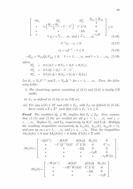
99
−Wq Π1ij Π3
ij
Bwi + Bwj
2
⋆ τ3
(
Wi + Wj
2− U − U
′)
U′
L′
Ω 0
⋆ ⋆ −2∆ 0⋆ ⋆ ⋆ −τ4R
≤ 0
∀ q, i = 1, . . . , nr and j = i, . . . , nr (5.16)
δ−1τ2 − τ1 < 0 (5.17)
τ3 + τ4δ−1 − 1 ≤ 0 (5.18)
−φ2ℓ + NℓQiN
′
ℓ ≤ 0, ∀ i = 1, . . . , nr and ℓ = 1, . . . , nφ (5.19)
whereΠ1
ij = 0.5 (AiU + BiY1j + AjU + BjY1i) ,
Π2ij = 0.5 (Qi + Qj) − U − U
′
,
Π3ij = 0.5 (Gi∆ + BiY2j + Gj∆ + BjY2i) .
Let Ki = Y1iU−1 and Γi = Y2i∆−1 for i = 1, . . . , nr. Then, the follo-
wing holds:
i) The closed-loop system consisting of (2.1) and (5.3) is locally UBstable;
ii) EI as defined in (5.14) is an UB set;
iii) For any w(k) ∈ W and x(0) ∈ EE, with EE as defined in (5.14),there exists a k ∈ Z+ such that x(k) ∈ EI , ∀ k ≥ k.
Proof The condition Qi ≥ Wi implies that EI ⊆ EE. Now, assumethat (5.15) and (5.16) are verified for all q, i = 1, . . . , nr and j =i, . . . , nr. Replace Y1i and Y2i respectively by KiU and Γi∆. Multiplythe resulting inequalities successively by h(i)(k), h(j)(k), h(q)(k + 1),and sum up on i, q = 1, . . . , nr and j = i, . . . , nr. Thus, the inequalitiesM1(h(k)) < 0 and M2(h(k)) < 0 holds if h(k) ∈ Ξ with
M1(h)=
−Q(h+) A(h)U G(h)∆ Bw(h) 0⋆ −U
′
Q−1(h)U U′
L′
Ω 0 U′
τ1
⋆ ⋆ −2∆ 0 0⋆ ⋆ ⋆ −τ2R 0⋆ ⋆ ⋆ ⋆ −τ1W (h)
,
M2(h)=
−W (h+) A(h)U G(h)∆ Bw(h)⋆ −τ3U
′
W (h)U U′
L′
Ω 0⋆ ⋆ −2∆ 0⋆ ⋆ ⋆ −τ4R
,
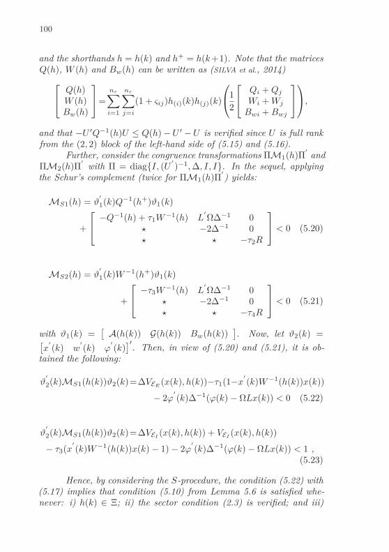
100
and the shorthands h = h(k) and h+ = h(k+1). Note that the matricesQ(h), W (h) and Bw(h) can be written as (SILVA et al., 2014)
Q(h)W (h)Bw(h)
=nr∑
i=1
nr∑
j=i
(1 + ςij)h(i)(k)h(j)(k)
1
2
Qi + Qj
Wi + Wj
Bwi + Bwj
,
and that −U ′Q−1(h)U ≤ Q(h) − U ′ − U is verified since U is full rankfrom the (2, 2) block of the left-hand side of (5.15) and (5.16).
Further, consider the congruence transformations ΠM1(h)Π′
andΠM2(h)Π
′
with Π = diagI, (U′
)−1, ∆, I, I. In the sequel, applyingthe Schur’s complement (twice for ΠM1(h)Π
′
) yields:
MS1(h) = ϑ′
1(k)Q−1(h+)ϑ1(k)
+
−Q−1(h) + τ1W −1(h) L′
Ω∆−1 0⋆ −2∆−1 0⋆ ⋆ −τ2R
< 0 (5.20)
MS2(h) = ϑ′
1(k)W −1(h+)ϑ1(k)
+
−τ3W −1(h) L′
Ω∆−1 0⋆ −2∆−1 0⋆ ⋆ −τ4R
< 0 (5.21)
with ϑ1(k) =[
A(h(k)) G(h(k)) Bw(h(k))]
. Now, let ϑ2(k) =[
x′
(k) w′
(k) ϕ′
(k)]′
. Then, in view of (5.20) and (5.21), it is ob-tained the following:
ϑ′
2(k)MS1(h(k))ϑ2(k)=∆VEE(x(k), h(k))−τ1(1−x
′
(k)W −1(h(k))x(k))
− 2ϕ′
(k)∆−1(ϕ(k) − ΩLx(k)) < 0 (5.22)
ϑ′
2(k)MS1(h(k))ϑ2(k)=∆VEI(x(k), h(k)) + VEI
(x(k), h(k))
− τ3(x′
(k)W −1(h(k))x(k) − 1) − 2ϕ′
(k)∆−1(ϕ(k) − ΩLx(k)) < 1 ,(5.23)
Hence, by considering the S-procedure, the condition (5.22) with(5.17) implies that condition (5.10) from Lemma 5.6 is satisfied whe-never: i) h(k) ∈ Ξ; ii) the sector condition (2.3) is verified; and iii)
101
assuming that x(k) does not leave X , for all k ≥ 0. The same proce-dure can be extended to (5.23) with (5.18) resulting in the verificationof (5.11).
Now, is required to show that x(k) ∈ X , for all k ≥ 0, andconsequently h(k) ∈ Ξ. To this end, assume that (5.19) is verified.Then, multiplying (5.19) by h(i)(k) and summing up on i = 1, . . . , nr
leads to:−φ2
ℓ + NℓQ(h(k))N′
ℓ ≤ 0,
which is equivalent to (see Klug, Castelan & Coutinho (2015a))
N′
ℓ(φ2ℓ)−1Nℓ − Q−1(h(k)) ≤ 0.
Pre- and post-multiplying the above respectively by x′
(k) and x(k) andconsidering the S-procedure leads to:
x′
(k)N′
ℓφ−2ℓNℓx(k) ≤ 1, ∀ x(k) ∈ EE
That is, E(Q−1i ) ⊂ X , ∀i = 1, ..., nr. Therefore it is ensured that x(k)
does not leave X , for all k ≥ 0, which concludes the proof.
Notice that the conditions of Theorem 5.7 are LMI constraintsif the positive scalars τ1 and τ3 are given a priori. To obtain a lessconservative result, a griding technique can be applied to determinethese parameters taking into account that τ3 ∈]0, 1[ due to the scalarinequality in (5.18). To avoid a possible large computational effort, it ispossible to constraint the sets EE and EI to have the same shape (i.e.,the set EE is a scaled version of EI). As a result, the only parameterto be searched is τ1 in a bounded space. Thus, the sets EE and EI areredefined as follows:
EE=
⋂
i∈1,...nr
E(
Q−1i , c−1
)
, EI=
⋂
i∈1,...nr
E(
Q−1i , 1
)
, (5.24)
where the nr ellipsoidal sets E(
Q−1i , c−1
)
are as follows:
E(
Q−1i , c−1
)
=
x(k) ∈ ℜn : x′
(k)Q−1i x(k) ≤ c−1 , c−1 ≥ 1
(5.25)
for i = 1, . . . , nr and with c being a parameter defining the size of EE .Therefore, the stabilization conditions proposed in Theorem 5.7
are simplified to the following result.
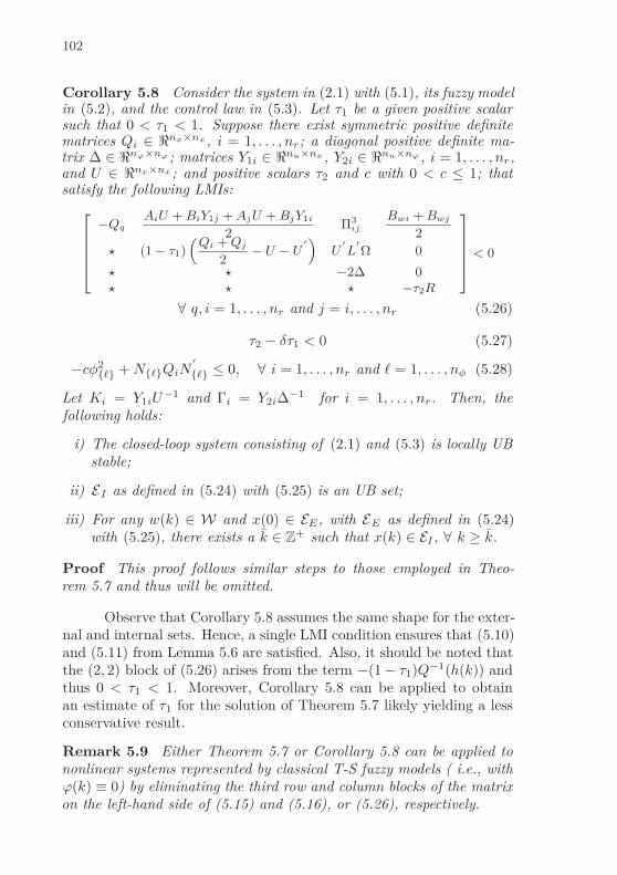
102
Corollary 5.8 Consider the system in (2.1) with (5.1), its fuzzy modelin (5.2), and the control law in (5.3). Let τ1 be a given positive scalarsuch that 0 < τ1 < 1. Suppose there exist symmetric positive definitematrices Qi ∈ ℜnx×nx , i = 1, . . . , nr; a diagonal positive definite ma-trix ∆ ∈ ℜnϕ×nϕ ; matrices Y1i ∈ ℜnu×nx , Y2i ∈ ℜnu×nϕ , i = 1, . . . , nr,and U ∈ ℜnx×nx ; and positive scalars τ2 and c with 0 < c ≤ 1; thatsatisfy the following LMIs:
−QqAiU + BiY1j + AjU + BjY1i
2Π3
ij
Bwi + Bwj
2
⋆ (1 − τ1)(
Qi + Qj
2− U − U
′)
U′
L′
Ω 0
⋆ ⋆ −2∆ 0⋆ ⋆ ⋆ −τ2R
< 0
∀ q, i = 1, . . . , nr and j = i, . . . , nr (5.26)
τ2 − δτ1 < 0 (5.27)
−cφ2ℓ + NℓQiN
′
ℓ ≤ 0, ∀ i = 1, . . . , nr and ℓ = 1, . . . , nφ (5.28)
Let Ki = Y1iU−1 and Γi = Y2i∆−1 for i = 1, . . . , nr. Then, the
following holds:
i) The closed-loop system consisting of (2.1) and (5.3) is locally UBstable;
ii) EI as defined in (5.24) with (5.25) is an UB set;
iii) For any w(k) ∈ W and x(0) ∈ EE, with EE as defined in (5.24)with (5.25), there exists a k ∈ Z+ such that x(k) ∈ EI , ∀ k ≥ k.
Proof This proof follows similar steps to those employed in Theo-rem 5.7 and thus will be omitted.
Observe that Corollary 5.8 assumes the same shape for the exter-nal and internal sets. Hence, a single LMI condition ensures that (5.10)and (5.11) from Lemma 5.6 are satisfied. Also, it should be noted thatthe (2, 2) block of (5.26) arises from the term −(1 − τ1)Q−1(h(k)) andthus 0 < τ1 < 1. Moreover, Corollary 5.8 can be applied to obtainan estimate of τ1 for the solution of Theorem 5.7 likely yielding a lessconservative result.
Remark 5.9 Either Theorem 5.7 or Corollary 5.8 can be applied tononlinear systems represented by classical T-S fuzzy models ( i.e., withϕ(k) ≡ 0) by eliminating the third row and column blocks of the matrixon the left-hand side of (5.15) and (5.16), or (5.26), respectively.

103
5.2.2 Dynamic Output Feedback
Let the following FLF’s:
VI(ξ(k), h(k)) = ξ′
(k)W−1(h(k))ξ(k),
VE(ξ(k), h(k)) = ξ′
(k)Q−1(h(k))ξ(k), (5.29)
with
W(h(k)) =nr∑
i=1
h(i)(k)Wi , Q(h(k)) =nr∑
i=1
h(i)(k)Qi , (5.30)
and Wi,Qi ∈ ℜ2nx×2nx are symmetric matrices to be determined fori = 1, . . . , nr.
Accordingly, the internal and external sets characterizing the UBstability are redefined as follows:
EaI ,
⋂
i∈1,...nr
E(W−1i ) , Ea
E ,⋂
i∈1,...nr
E(Q−1i ) , (5.31)
with E(W−1i ) and E(Q−1
i ) being ellipsoidal sets as defined below:
E(W−1i ) =
ξ(k) ∈ ℜ2nx : ξ′
(k)W−1i ξ(k) ≤ 1
,
E(Q−1i ) =
ξ(k) ∈ ℜ2nx : ξ′
(k)Q−1i ξ(k) ≤ 1
.(5.32)
Also, the T-S domain of validity is redefined in terms of the augmentedspace (equal to the definition (3.10) in Chapter 3):
X a = ξ(k) ∈ ℜ2nx : |Nξ(k)| φ, (5.33)
where N = [ N 0nφ×nx].
Similarly to the procedure performed in Chapter 3, section 3.3,consider nx-dimensional real square matrices X, Y , P and Z such thatthe following matrices are nonsingular:
U =
[
X •Z •
]
, U−1 =
[
Y •P •
]
, Θ =
[
Y In
P 0
]
, (5.34)
with • denoting any real matrix with compatible dimensions. In viewof the above definitions, note that:

104
UΘ =
[
In X0 Z
]
.
Hence, the parametrization Θ′UΘ yields:
U = Θ′UΘ =
[
Y ′ T ′
In X
]
, T ′ = Y ′X + P ′Z . (5.35)
Furthermore, partitioning the matrices Qi and Wi as follows:
Qi =
[
Q11i Q12i
⋆ Q22i
]
, Wi =
[
W11i W12i
⋆ W22i
]
leads to :
Qi =Θ′QiΘ=
Y ′Q11iY + P ′Q′12iY +
Y ′Q12iP + P ′Q22iPY ′Q11i+P ′Q′
12i
⋆ Q11i
=
[
Q11i Q12i
⋆ Q22i
]
.
Wi =Θ′WiΘ=
Y ′W11iY + P ′W ′12iY +
Y ′W12iP + P ′W22iPY ′W11i+P ′W ′
12i
⋆ W11i
=
[
W11i W12i
⋆ W22i
]
.
Then, the following result is proposed to determine the matricesof the dynamic output feedback controller (5.5).
Theorem 5.10 Consider the nonlinear system in (2.1), its N-fuzzyrepresentation in (5.2) with h(k) = h(y(k)), and the controller definedin (5.5). Let the positive scalars τ1 and τ3 ∈ (0, 1), and a diagonalpositive definite matrix ∆ ∈ ℜnϕ×nϕ . Suppose there exist symmetricpositive definite matrices Qi, Wi ∈ ℜ2nx×2nx , i = 1, . . . , nr; matricesX, Y , T , Aij, Bij, Ci, Di of appropriate dimensions; and positive
scalars τ2 and τ4; that satisfy Qi ≥ Wi and the following LMIs:
−Qq Π1ij Π2
ij Π3ij 0
⋆Qi+Qj
2−U−U
′L
′
Ω
X′
L′
Ω
0 τ1U′
⋆ ⋆−2∆
0
0
−τ2R
0
⋆ ⋆ ⋆ ⋆ −τ1
(
Wi+Wj
2
)
< 0
∀ q, i = 1, ..., nr and j = i, ..., nr (5.36)

105
−τ1 + τ2δ−1 < 0 (5.37)
−Wq Π1ij Π2
ij Π3ij
⋆ τ3
(
Wi + Wj
2− U − U
′
)
L′
Ω
X′
L′
Ω
0
⋆ ⋆−2∆
0
0
−τ4R
≤ 0
∀ q, i = 1, ..., nr and j = i, ..., nr (5.38)
τ3 + τ4δ−1 − 1 ≤ 0 (5.39)
−Qi + U + U′ N
′
ℓ
(NX)′
ℓ
⋆ φ2ℓ
> 0,
∀ i = 1, ..., nr and ℓ = 1, ..., nφ (5.40)
where U is as in (5.35) and
Π1ij =
Y′
(Ai + Aj) + BijC
2
Aij
2Ai + Aj + (BiDj + BjDi)C
2
(Ai + Aj)X + BiCj + BjCi
2
,
Π2ij =
Y′(
Gi + Gj
2
)
∆(
Gi + Gj
2
)
∆
,
Π3ij =
[
Bwi + Bwj
20
]
.
Let P be any nonsingular matrix and define the following matrices:
Z = (P ′)−1(T ′ − Y ′X), Dci=Di
Cci = (Ci − DciCX)Z−1,
Bcij = (P ′)−1[
Bij − Y ′(BiDcj + BjDci)]
,
Acij = (P ′)−1[
Aij −Y ′(Ai + Aj)X−BijCX−Y ′(BiCcj +BjCci)Z]
Z−1,
(5.41)
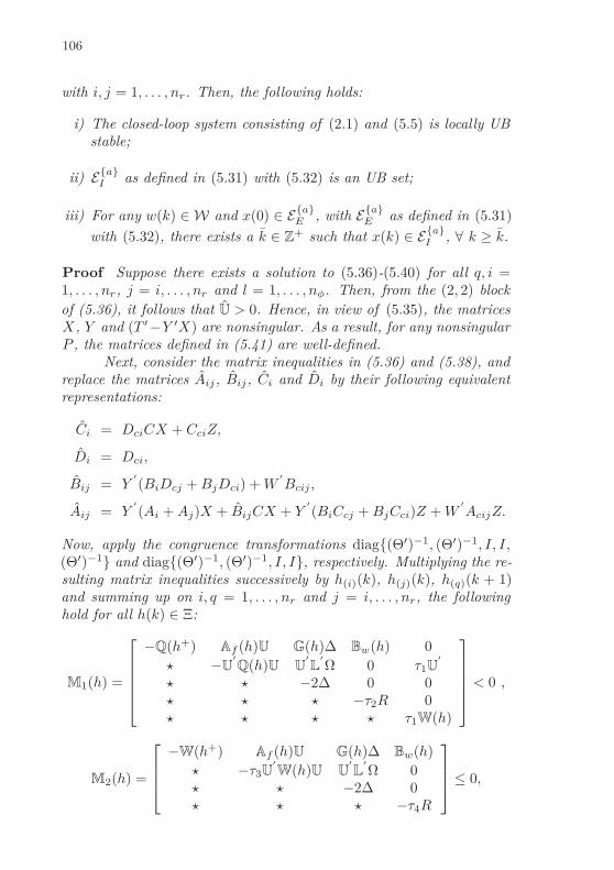
106
with i, j = 1, . . . , nr. Then, the following holds:
i) The closed-loop system consisting of (2.1) and (5.5) is locally UBstable;
ii) EaI as defined in (5.31) with (5.32) is an UB set;
iii) For any w(k) ∈ W and x(0) ∈ EaE , with Ea
E as defined in (5.31)
with (5.32), there exists a k ∈ Z+ such that x(k) ∈ EaI , ∀ k ≥ k.
Proof Suppose there exists a solution to (5.36)-(5.40) for all q, i =1, . . . , nr, j = i, . . . , nr and l = 1, . . . , nφ. Then, from the (2, 2) block
of (5.36), it follows that U > 0. Hence, in view of (5.35), the matricesX, Y and (T ′ −Y ′X) are nonsingular. As a result, for any nonsingularP , the matrices defined in (5.41) are well-defined.
Next, consider the matrix inequalities in (5.36) and (5.38), andreplace the matrices Aij, Bij, Ci and Di by their following equivalentrepresentations:
Ci = DciCX + CciZ,
Di = Dci,
Bij = Y′
(BiDcj + BjDci) + W′
Bcij ,
Aij = Y′
(Ai + Aj)X + BijCX + Y′
(BiCcj + BjCci)Z + W′
AcijZ.
Now, apply the congruence transformations diag(Θ′)−1, (Θ′)−1, I, I,(Θ′)−1 and diag(Θ′)−1, (Θ′)−1, I, I, respectively. Multiplying the re-sulting matrix inequalities successively by h(i)(k), h(j)(k), h(q)(k + 1)and summing up on i, q = 1, . . . , nr and j = i, . . . , nr, the followinghold for all h(k) ∈ Ξ:
M1(h) =
−Q(h+) Af (h)U G(h)∆ Bw(h) 0⋆ −U
′
Q(h)U U′
L′
Ω 0 τ1U′
⋆ ⋆ −2∆ 0 0⋆ ⋆ ⋆ −τ2R 0⋆ ⋆ ⋆ ⋆ τ1W(h)
< 0 ,
M2(h) =
−W(h+) Af (h)U G(h)∆ Bw(h)⋆ −τ3U
′
W(h)U U′
L′
Ω 0⋆ ⋆ −2∆ 0⋆ ⋆ ⋆ −τ4R
≤ 0,
107
with Af (h) = A(h) +B(h)K(h) and the shorthands h = h(k) and h+ =h(k + 1).
The rest of this proof follows from the proof of Theorem 4.4.
5.3 DESIGN ISSUES
In this section the controllers design based on the previous resultsis proposed through optimization problems, which aims: i) to obtainthe smallest UB set EI ; or ii) to obtain the set of initial conditions EE
that cover as much as possible the domain of validity X ; and iii) toconsider the two previous objectives into a multiobjective problem.
5.3.1 State and Sector Nonlinearities Feedback Design
5.3.1.1 Minimization of EI
In this case the objective consists in minimizing the UB set EI .For this purpose the set EI will be included in the sphere with radius
equal to√
γ, which will be minimized. Then, EI ⊆ E(
1
γInx
)
⇔
x′
(k)1
γInx
x(k) ≤ 1 ∀ x′
(k)W −1(h(k))x(k) ≤ 1, which can be equiva-
lently represented by (DILDA; JUNGERS; CASTELAN, 2014):
[
γInxWi
⋆ Wi
]
≥ 0
∀ i = 1, ..., nr
(5.42)
Thus, the following convex optimization problem is proposed:
min γQi, Wi, ∆, Y1i, Y2i, U, τ2, τ4
subject toLMIs (5.15), (5.16), (5.17) , (5.18), (5.19) and (5.42).
(5.43)
5.3.1.2 Maximization of EE
Ideally, the set of initial conditions should be coincident with thedomain of validity X . However, to ensure that the system trajectories

108
do not evolve outside this domain (where T-S model convexity cannotbe guaranteed), the set EE represents the admissible region of initialconditions. In this way, the objective is to maximize the set EE ⊆ X .For this purpose, it is considered that X can be described by
X = Co vσ ∈ ℜnx , σ = 1, ..., nσ
where the set of vectors vσ ∈ ℜnx contain the information nece-ssary to characterize the shape of X . Then, the objective consists inmaximizing the factor β such that the inclusion βX ⊆ EE is verified.Considering µ = 1/β2, this inclusion is equivalent to
[
µ v′
σ
⋆ Qi
]
≥ 0
∀ i = 1, ..., nr and σ = 1, ..., nσ
(5.44)
In this case, the following convex optimization problem is proposed:
min µQi, Wi, ∆, Y1i, Y2i, U, τ2, τ4
subject toLMIs (5.15), (5.17), (5.16), (5.18), (5.19) and (5.44).
(5.45)
5.3.1.3 Multiobjective Problem
It is possible to formulate a multiobjective optimization problemfor considering the previous objectives at the cost of losing convexity.A nonconvex optimization is hard to be solved and approximate con-vex solutions might be applied to this end. In this way, the followingapproximate multiobjective optimization problem is proposed:
min λγ + (1 − λ)µQi, Wi, ∆, Y1i, Y2i, U, τ2, τ4
subject toLMIs (5.15), (5.17), (5.16), (5.18), (5.19), (5.42) and (5.44).
(5.46)Observe that the design parameter λ ∈ [0, 1] is responsible for weightingeach objective.
Remark 5.11 Notice that in any of the above optimization problems,it is required to perform a search in space τ1 × τ3 ∈ ]0, 1[, to select thevalues that yields the best optimized objective, as will be illustrated inthe experiments section.
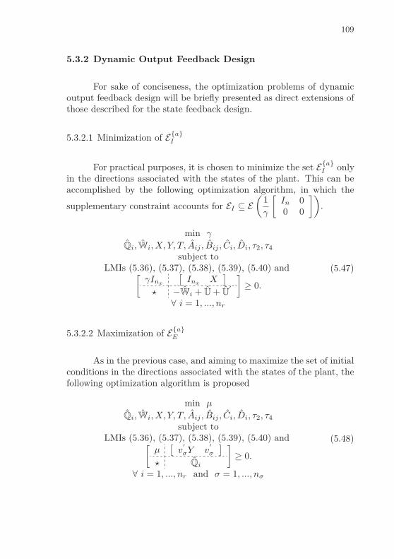
109
5.3.2 Dynamic Output Feedback Design
For sake of conciseness, the optimization problems of dynamicoutput feedback design will be briefly presented as direct extensions ofthose described for the state feedback design.
5.3.2.1 Minimization of EaI
For practical purposes, it is chosen to minimize the set EaI only
in the directions associated with the states of the plant. This can beaccomplished by the following optimization algorithm, in which the
supplementary constraint accounts for EI ⊆ E(
1
γ
[
In 00 0
])
.
min γ
Qi, Wi, X, Y, T, Aij , Bij , Ci, Di, τ2, τ4
subject toLMIs (5.36), (5.37), (5.38), (5.39), (5.40) and
[
γInx
[
InxX]
⋆ −Wi + U + U′
]
≥ 0.
∀ i = 1, ..., nr
(5.47)
5.3.2.2 Maximization of EaE
As in the previous case, and aiming to maximize the set of initialconditions in the directions associated with the states of the plant, thefollowing optimization algorithm is proposed
min µ
Qi, Wi, X, Y, T, Aij , Bij , Ci, Di, τ2, τ4
subject toLMIs (5.36), (5.37), (5.38), (5.39), (5.40) and
[
µ[
v′
σY v′
σ
]
⋆ Qi
]
≥ 0.
∀ i = 1, ..., nr and σ = 1, ..., nσ
(5.48)

110
5.3.2.3 Multiobjetive Problem
The approximate multiobjective optimization problem blends(5.47) and (5.48) in the same way as in (5.46), with the weightingparameter λ ∈ [0, 1]. As a result, the following convex optimizationproblem is proposed:
min λγ + (1 − λ)µQi, Wi, X, Y, T, Aij , Bij , Ci, Di, τ2, τ4
subject toLMIs (5.36), (5.37), (5.38), (5.39), (5.40),
[
γInx
[
InxX]
⋆ −Wi + U + U′
]
≥ 0
∀ i=1, ..., nr
and
[
µ[
v′
σY v′
σ
]
⋆ Qi
]
≥ 0.
∀ i=1, ..., nr and σ = 1, ..., nσ
(5.49)
5.4 EXPERIMENTS
Consider the two dimensional nonlinear system presented in Ap-pendix B, section B.4. The state space representation of the system isgiven by:
x(1)(k + 1) =3
10x(1)(k)−
1
2x(2)(k)−
1
10x
2(1)(k)+
1
4x(1)(k)x(2)(k)
+3
10x(2)(k)(1 + sin(x(2)(k)))+
7
10u(k)+
1
20x(1)(k)u(k)
−1
2w(1)(k)−
1
4x(1)(k)w(1)(k)−
11
20w(2)(k)+
7
40x(1)(k)w(2)(k)
x(2)(k + 1) =1
20x(1)(k)−
3
10x(2)(k)+
9
40x
2(1)(k)−
1
10x(1)(k)x(2)(k)
−1
20u(k)+
1
40x(1)(k)u(k)+
9
10w(1)(k)+
9
20x(1)(k)w(1)(k)
+1
20w(2)(k)+
19
40x(1)(k)w(2)(k)
(5.50)
The above nonlinear system will be used to demonstrate thepotential of the described approach as a control design tool for nonlineardiscrete-time systems subject to persistent disturbances. To this end,it is considered that the states are constrained in the domain definedby |x(1)(k)| ≤ 2 and |x(2)(k)| ≤ 1.5, and that disturbance vector liesinside the set W, in (5.1), defined by δ = 20 and R = diag13.88, 20.Figure 24 shows a particular disturbance vector wk ∈ W used in thesimulations.
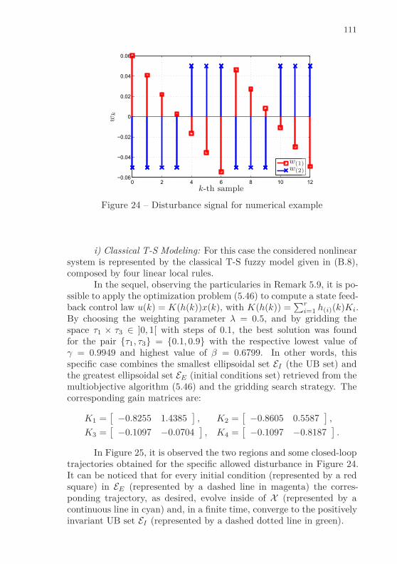
111
0 2 4 6 8 10 12−0.06
−0.04
−0.02
0
0.02
0.04
0.06
k-th sample
wk
w(1)w(2)
Figure 24 – Disturbance signal for numerical example
i) Classical T-S Modeling: For this case the considered nonlinearsystem is represented by the classical T-S fuzzy model given in (B.8),composed by four linear local rules.
In the sequel, observing the particularies in Remark 5.9, it is po-ssible to apply the optimization problem (5.46) to compute a state feed-back control law u(k) = K(h(k))x(k), with K(h(k)) =
∑ri=1 h(i)(k)Ki.
By choosing the weighting parameter λ = 0.5, and by gridding thespace τ1 × τ3 ∈ ]0, 1[ with steps of 0.1, the best solution was foundfor the pair τ1, τ3 = 0.1, 0.9 with the respective lowest value ofγ = 0.9949 and highest value of β = 0.6799. In other words, thisspecific case combines the smallest ellipsoidal set EI (the UB set) andthe greatest ellipsoidal set EE (initial conditions set) retrieved from themultiobjective algorithm (5.46) and the gridding search strategy. Thecorresponding gain matrices are:
K1 =[
−0.8255 1.4385]
, K2 =[
−0.8605 0.5587]
,
K3 =[
−0.1097 −0.0704]
, K4 =[
−0.1097 −0.8187]
.
In Figure 25, it is observed the two regions and some closed-looptrajectories obtained for the specific allowed disturbance in Figure 24.It can be noticed that for every initial condition (represented by a redsquare) in EE (represented by a dashed line in magenta) the corres-ponding trajectory, as desired, evolve inside of X (represented by acontinuous line in cyan) and, in a finite time, converge to the positivelyinvariant UB set EI (represented by a dashed dotted line in green).
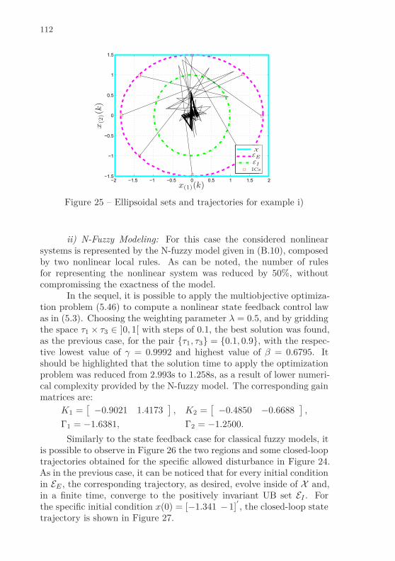
112
−2 −1.5 −1 −0.5 0 0.5 1 1.5 2−1.5
−1
−0.5
0
0.5
1
1.5
x(1)(k)
x(2
)(k
)
X
EE
EIICs
Figure 25 – Ellipsoidal sets and trajectories for example i)
ii) N-Fuzzy Modeling: For this case the considered nonlinearsystems is represented by the N-fuzzy model given in (B.10), composedby two nonlinear local rules. As can be noted, the number of rulesfor representing the nonlinear system was reduced by 50%, withoutcompromissing the exactness of the model.
In the sequel, it is possible to apply the multiobjective optimiza-tion problem (5.46) to compute a nonlinear state feedback control lawas in (5.3). Choosing the weighting parameter λ = 0.5, and by griddingthe space τ1 × τ3 ∈ ]0, 1[ with steps of 0.1, the best solution was found,as the previous case, for the pair τ1, τ3 = 0.1, 0.9, with the respec-tive lowest value of γ = 0.9992 and highest value of β = 0.6795. Itshould be highlighted that the solution time to apply the optimizationproblem was reduced from 2.993s to 1.258s, as a result of lower numeri-cal complexity provided by the N-fuzzy model. The corresponding gainmatrices are:
K1 =[
−0.9021 1.4173]
, K2 =[
−0.4850 −0.6688]
,
Γ1 = −1.6381, Γ2 = −1.2500.
Similarly to the state feedback case for classical fuzzy models, itis possible to observe in Figure 26 the two regions and some closed-looptrajectories obtained for the specific allowed disturbance in Figure 24.As in the previous case, it can be noticed that for every initial conditionin EE , the corresponding trajectory, as desired, evolve inside of X and,in a finite time, converge to the positively invariant UB set EI . Forthe specific initial condition x(0) = [−1.341 −1]
′
, the closed-loop statetrajectory is shown in Figure 27.

113
−2 −1.5 −1 −0.5 0 0.5 1 1.5 2−1.5
−1
−0.5
0
0.5
1
1.5
x(1)(k)
x(2
)(k
)
X
EE
EIICs
Figure 26 – Ellipsoidal sets and trajectories for example ii)
0 2 4 6 8 10 12−1.5
−1
−0.5
0
0.5
1
k-th sample
x(k
)
x(1)x(2)
Figure 27 – State trajectories for example ii)
At last, by comparing the associated values of γ and β, and bycomparing Figures 25 and 26, it can be seen that there is no significantqualitative difference between the two solution.
iii) Output Feedback: In previous numerical experiments, thestate variables x(1)(k) and x(2)(k) were assumed to be measurable, allo-wing the implementation of fuzzy control laws that depend of h(k) =h(x(1)(k), x(2)(k)) when designed from the classical T-S model, or ofh(k) = h(x(1)(k)) and ϕ(k) = ϕ(x(2)(k)) when designed from the N-fuzzy model.
Next, to show how the proposed dynamic output feedback stra-
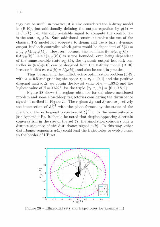
114
tegy can be useful in practice, it is also considered the N-fuzzy modelin (B.10), but additionally defining the output equation by y(k) =[1 0] x(k), i.e., the only available signal to compute the control lawis the state x(1)(k). Such additional constraint makes the use of theclassical T-S model not adequate to design and use a fuzzy dynamicoutput feedback controller which gains would be dependent of h(k) =h(x(1)(k), x(2)(k)). However, because the nonlinearity ϕ(x(2)(k)) =0.3x(2)(k)(1 + sin(x(2)(k))) is sector bounded, even being dependentof the unmeasurable state x(2)(k), the dynamic output feedback con-troller in (5.5)-(5.6) can be designed from the N-fuzzy model (B.10),because in this case h(k) = h(y(k)), and also be used in practice.
Thus, by applying the multiobjective optimization problem (5.49),with λ = 0.5 and gridding the space τ1 × τ3 ∈ ]0, 1[ and the positivediagonal matrix ∆, we obtain the lowest value of γ = 1.8345 and thehighest value of β = 0.6228, for the triple τ1, τ3, ∆ = 0.1, 0.8, 2.
Figure 28 shows the regions obtained for the above-mentionedproblem and some closed-loop trajectories considering the disturbancesignals described in Figure 24. The regions EE and EI are respectivelythe intersection of Ea
E with the plane formed by the states of the
plant and the orthogonal projection of EaI onto the same subspace
(see Appendix E). It should be noted that despite appearing a certainconservatism in the size of the set EI , the simulation considers only adistinct sequence of the disturbance signal w(k). In this way, otherdisturbance sequences w(k) could lead the trajectories to evolve closerto the border of UB set.
−2 −1.5 −1 −0.5 0 0.5 1 1.5 2−1.5
−1
−0.5
0
0.5
1
1.5
x(1)(k)
x(2
)(k
)
X
EE
EIICs
Figure 28 – Ellipsoidal sets and trajectories for example iii)

115
In Figure 29, it is shown the state trajectories for the initialcondition x(0) = [1.77 0]
′
and xc(0) = [0 0]′
. Notice that the over-all performance is similar to that achieved with the state and sectornonlinearity feedback.
0 2 4 6 8 10 12−0.5
0
0.5
1
1.5
2
k-th sample
x(k
)
x(1)x(2)
Figure 29 – State trajectories for example iii)
5.5 CONCLUDING REMARKS
In this chapter a convex approach for the design of fuzzy con-trollers that locally stabilizes nonlinear discrete-time systems subjectto amplitude bounded disturbances was presented. Considering fuzzyLyapunov functions, optimization problems in terms of LMI constraintswere proposed to design a nonlinear state-feedback control law, whichis a function of the membership fuzzy functions and cone sector non-linearities, and to design a dynamic output feedback control law. Aninteresting characteristic is that the dynamic output case admits theexistence of nonlinearities with unmeasured states in the original sys-tem, as opposed to the classical literature strategies and the approachlately proposed in Chapter 3. Additionally, two ellipsoidal sets, EE andEI , are taken into account, associated respectively to the admissibleregion of initial conditions and the concept of ultimate bounded . Boththe theoretical developments and the design strategies consider thatthe convexity of the fuzzy models holds in a given domain of validity.

116

6 INTERACTIVE SOFTWARE AND HARDWAREIMPLEMENTATION
Chapters 2, 3, 4 and 5 provide theoretical tools for modeling andcontrol of nonlinear systems via T-S fuzzy approach. In this chapter,aiming to assist students, researches and engineers in the control designof nonlinear systems using FMB techniques, the following results areproposed:
i) an interactive software for modeling and control of nonlinear sys-tems, and
ii) a Hardware-in-the-Loop (HIL) implementation is applied to evalu-ate the digital implementation of T-S fuzzy controllers.
The proposed interactive software is a Matlab-based toolbox freelyavailable for the scientific community which provides a user-friendly in-teractive environment for modeling and control of nonlinear systemsconsidering FMB approaches. The fuzzy toolbox is summarized in thereference Klug, Castelan & Coutinho (2015a).
The second result of this chapter regards practical aspects of adigital implementation of T-S fuzzy controllers. More specifically, avirtual plant runs over an Matlab/Simulink environment and a digitalcontroller is built over a FPGA (Field Programmable Gate Array) de-velopment board which communicates with the virtual plant using aEthernet network. These results are summarized in the reference Kluget al. (2014).
This chapter is organized as follows: in Section 6.1, the detailsof the interactive software operation, as well as its modules and possi-ble configurations are discussed. Section 6.2 deals with the hardwareimplementation, specifying the programming platform to be used andthe HIL structure, and resulting in a comparative example. Finally,the conclusions of this chapter are presented in Section 6.3.
6.1 INTERACTIVE SOFTWARE FOR MODELING AND CONTROLDESIGN
The mathematical modeling of dynamical systems is an impor-tant research field in automatic control (GUZMAN et al., 2008). An ana-lytical model is essential for running simulations and designing model-based control systems, despite, in many cases, not representing every
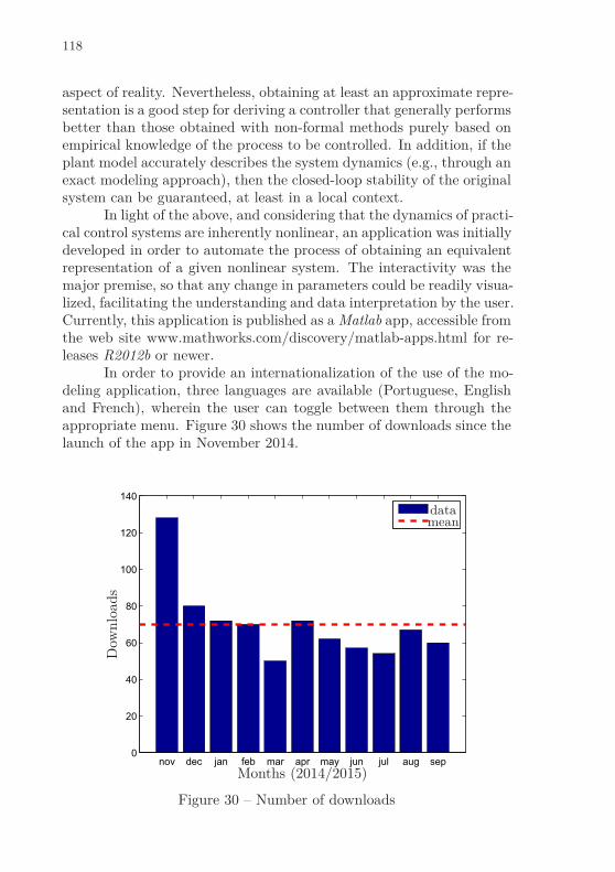
118
aspect of reality. Nevertheless, obtaining at least an approximate repre-sentation is a good step for deriving a controller that generally performsbetter than those obtained with non-formal methods purely based onempirical knowledge of the process to be controlled. In addition, if theplant model accurately describes the system dynamics (e.g., through anexact modeling approach), then the closed-loop stability of the originalsystem can be guaranteed, at least in a local context.
In light of the above, and considering that the dynamics of practi-cal control systems are inherently nonlinear, an application was initiallydeveloped in order to automate the process of obtaining an equivalentrepresentation of a given nonlinear system. The interactivity was themajor premise, so that any change in parameters could be readily visua-lized, facilitating the understanding and data interpretation by the user.Currently, this application is published as a Matlab app, accessible fromthe web site www.mathworks.com/discovery/matlab-apps.html for re-leases R2012b or newer.
In order to provide an internationalization of the use of the mo-deling application, three languages are available (Portuguese, Englishand French), wherein the user can toggle between them through theappropriate menu. Figure 30 shows the number of downloads since thelaunch of the app in November 2014.
nov dec jan feb mar apr may jun jul aug sep0
20
40
60
80
100
120
140
Months (2014/2015)
Dow
nlo
ads
datamean
Figure 30 – Number of downloads

119
It can be noted that after an elevated number of downloads in thefirst month, that number remained near the average thereafter. Thisdemand, coupled with the comments received during the lecture enti-tled “Control of Nonlinear Systems Using T-S Fuzzy Models: Theoryand Implementation”, offered in the Brazilian Conference on AutomaticControl - CBA 2014, led to the development of another application.This time the objective was the control design of fuzzy controllers.
For the control application, the basic idea is to automaticallyimport the fuzzy model originating from the modeling application, andobtain the gains of a particular controller that satisfy the closed-loopperformance requirements, after defining parameters and optimizationcriteria. Among the available library of control laws are the controllersdeveloped during the author’s doctoral studies. Further details on themodeling and control applications are presented in the following sub-sections.
6.1.1 Modeling Application
This application uses the theoretical fuzzy T-S modeling basispresented in Chapter 2, based on the works Teixeira & Zak (1999),Tanaka & Wang (2001), Feng (2010) and Klug & Castelan (2011). Theprogramming code uses symbolic math and string handling, amongother packages/toolboxes of the Matlab environment. The starting win-dow, shown in Figure 31, allows the user to select the type of modelingtechnique and the desired language.
Figure 31 – Initial window
Once the first configurations are defined in the starting window,the application is divided into two distinct modules, approximate andexact modeling, whose features are described below.

120
6.1.1.1 Approximate Modeling Module
In this module the approximate T-S fuzzy modeling approachpresented in Appendix A is used. Basically, the procedure is performedby choosing a finite number of Operation Points (OPs) which will beassociated with local linear submodels. These local submodels appro-ximately represent the behavior of the nonlinear plant in the neighbor-hood of the associated OPs, whose quantities and position are basedon the physical knowledge of the system dynamics and the desired ap-proximation error.
Thus, the approximate T-S fuzzy model is obtained by the in-terconnection of local submodels, provided by the use of membershipfunctions. These functions usually have a particular shape, such as tri-angular, trapezoidal, Gaussian or bell-shaped, and should respect theconvex sum property.
The main window of this module is illustrated in Figure 32 withthe following subdivisions (a menu and five panels):
Figure 32 – Approximate modeling module window
1. Menu: the user can access pre-defined examples, save and opena nonlinear system data, as well as change the language of theprogram.

121
2. Nonlinear System Panel: the user enters the analytical equationsof the nonlinear system, using, by default, pre-declared states x1
and x2.
3. Region of Operation Panel: the user can configure the regionof interest (via slide bars) and the desired number of operationpoints.
4. Fuzzy Rules Panel: the user can visualize the fuzzy rules.
5. Membership Functions Panel: it allows the user to change andvisualize the shape of the membership functions (not all typesare pre-programmed).
6. Open Loop Simulation: it allows the user to execute a compara-tive simulation with the original nonlinear plant and the respec-tive T-S fuzzy model.
The user interface was made to be intuitive. Once the nonlinearsystem is inserted and the operation region configured (quantity andpositioning of the OPs), the approximate fuzzy model is obtained bypressing the “Acquire T-S Model” button. In this way, the applicationcomputes the optimal local submodels and presents them in the “FuzzyRules Panel”, also allowing the user to export the final result in vari-ous formats, including .txt, .tex and .mat (required to use the controlsoftware) .
Finally, once the nonlinear system is modeled, the user can runan open loop simulation setting up the desired initial condition andthe number of samples. This simulation allows a comparative analysisof the trajectories emanating from the initial condition, representedby a square, of the original system with the fuzzy model, representedrespectively by the “+” and “” symbols.
In order to provide an evidence of how much each subsystemcontributes to the global fuzzy T-S model, each membership functionis represented with the same color as the associated operation point.This fact allows the user to observe which regions of the state spacewhere there is dominance from a particular membership function, andtherefore where each local submodel has a larger weight on the repre-sentation.
It is also important to emphasize that, as part of the desiredsoftware interactivity, following any changes in the settings/parametersthat generates the fuzzy model (such as the quantity and positioning ofthe OPs), all graphics are immediately rendered considering this new

122
conjuncture. This is an important feature for the control designer, fa-cilitating a suitable choice in the trade-off between the number of fuzzyrules and the numerical and implementation complexity, also associatedwith the accuracy of the representation.
6.1.1.2 Exact Modeling Module
In this part, the application allows to handle T-S fuzzy modelsthat accurately represent the original nonlinear system in a specificdomain of the state space. Notice that this module requires someknowledge of the user with the exact fuzzy modeling technique andit has more step configurations than the previous module. User-madechoices will determine whether the resulting model will have classicalor N-fuzzy structure.
The main window is observed in Figure 33. There is one menuand four panels which are identical to the ones described previously:panels 2, 5, 6 and 7. These panels are in accordance with the previouspanels 2, 4, 5 and 6. The following two panels have specific functions:
Figure 33 – Exact modeling module window
3. Validity Domain and Nonlinear Treatment Panel: the user setsthe desired domain of validity, where the model convexity is gua-ranteed, via slide bars. Then, fuzzification is performed separately
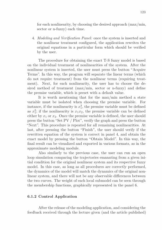
123
for each nonlinearity, by choosing the desired approach (max/min,sector or n-fuzzy) each time.
4. Modeling and Verification Panel: once the system is inserted andthe nonlinear treatment configured, the application rewrites theoriginal equations in a particular form which should be verifiedby the user.
The procedure for obtaining the exact T-S fuzzy model is basedon the individual treatment of nonlinearities of the system. After thenonlinear system is inserted, the user must press the button “AcquireTerms”. In this way, the program will separate the linear terms (whichdo not require treatment) from the nonlinear terms (requiring treat-ment). Next, for each nonlinearity, the user has to choose the de-sired method of treatment (max/min, sector or n-fuzzy) and definethe premise variable, which is preset with a default value.
It is worth mentioning that for the max/min method a statevariable must be isolated when choosing the premise variable. Forinstance, if the nonlinearity is x3
1, the premise variable must be definedas x2
1; if the nonlinearity is x1x2, the premise variable can be definedeither by x1 or x2. Once the premise variable is defined, the user shouldpress the button “Set PV / Plot”, verify the graph and press the button“Next”. This procedure is repeated for all remaining nonlinearities. Atlast, after pressing the button “Finish”, the user should verify if therewritten equation of the system is correct in panel 4, and obtain theexact model by pressing the button “Obtain Model”. In this way, thefinal result can be visualized and exported in various formats, as in theapproximate modeling module.
Also similarly to the previous case, the user can run an openloop simulation comparing the trajectories emanating from a given ini-tial condition for the original nonlinear system and its respective fuzzymodel. In this case, as long as all procedures are correctly performed,the dynamics of the model will match the dynamics of the original non-linear system, and there will not be any observable differences betweenthe two curves. The weight of each local submodel can be seen throughthe membership functions, graphically represented in the panel 6.
6.1.2 Control Application
After the release of the modeling application, and considering thefeedback received through the lecture given (and the article published)

124
at the XX-CBA 2014, a second Matlab-based application aiming thefuzzy controller design was developed. Thus, the two apps becomean interesting tool to study the control of nonlinear systems via T-Sfuzzy models. This is one of the contributions of this work, since veryfew similar works are found in the literature which systematizes thenonlinear control design in light of results found in the scope of Linear-Time Invariant (LTI) systems.
To use this application, it is necessary to have previously ob-tained the T-S fuzzy model with the modeling software (if necessary,the model can be manually inserted, using permitted notation and sym-bols). The program is able to load .mat files (a Matlab format) andcompute the controller gains based on a selected control law and a fewperformance requirements and optimization settings. The user musthave installed the Yalmip Interface, and solvers Sedumi and SPDT3.
Until now, the following fuzzy controllers are available: statefeedback, state and sector nonlinearity feedback, and dynamic outputfeedback, depending on how the system is represented (classical or N-fuzzy). These controllers are based on the work described in the pre-ceding chapters and in the articles Klug & Castelan (2011), Klug &Castelan (2012) and Klug et al. (2014).
Figure 34 shows the user’s interface window. The use of themenu is similar to the modeling application, allowing the user to loadpre-defined examples and change the language, among other features.The following panels have specific functions:
2. Fuzzy Model Loading Panel: the user has to import the fuzzymodel obtained with the modeling app or insert it manually usinga .mat file.
3. Controller Settings Panel: the user defines the desired control lawand the optimization objectives to be used.
4. Solver Settings Panel: it allows the user to choose the solver andits properties/settings.
5. Statistics Panel: it allows the user to visualize the data returnedby the solver in the solution of the optimization problem.
6. Simulation and Controller Gains Panel: it displays the controllergains and enables the execution of a closed-loop simulation.
The use of the app is simple. Once the fuzzy model data isloaded, the application identifies the type of model and the numberof rules, only enabling the relevant controllers, depending on how the
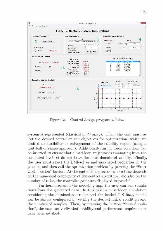
125
Figure 34 – Control design program window
system is represented (classical or N-fuzzy). Then, the user must se-lect the desired controller and objectives for optimization, which arelimited to feasibility or enlargement of the stability region (using aunit ball or shape approach). Additionally, an inclusion condition canbe inserted to ensure that closed-loop trajectories emanating from thecomputed level set do not leave the local domain of validity. Finally,the user must select the LMI-solver and associated properties in thepanel 4, and then call the optimization problem by pressing the “StartOptimization” button. At the end of this process, whose time dependson the numerical complexity of the control algorithm, and also on thenumber of rules, the controller gains are displayed in panel 6.
Furthermore, as in the modeling app, the user can run simula-tions from the generated data. In this case, a closed-loop simulationconsidering the obtained controller and the loaded T-S fuzzy modelcan be simply configured by setting the desired initial condition andthe number of samples. Then, by pressing the button “Start Simula-tion”, the user can verify that stability and performance requirementshave been satisfied.

126
6.2 HIL IMPLEMENTATION
In this section some aspects related to the practical implemen-tation of T-S fuzzy controllers on real platforms are considered. Forthis purpose, HIL simulations were performed comparing a controllerdeveloped in this thesis, and other found in literature. In this sense,the study of the computational burden to the digital implementation ofnonlinear control systems is evaluated using the classical and N-fuzzyapproaches.
The HIL simulation is a technique for the development and testof complex systems, typically used at the project level to design andtune a controller. It is common to simulate the dynamics of the plantin real-time, either because the physical prototype is not available orbecause real experiments of the project involve unnecessary costs incertain phases (development time and investment). The HIL frame-work is characterized by the combined use of real and simulated compo-nents/parts, where e.g. the hardware is the controller, and the softwareis a virtual simulation of the real system.
The platform chosen to embed the control law is the FPGA de-velopment board DE2−115, manufactured by Altera and illustrated inFigure 35. This board is equipped with the Cyclone EP4CE115F29C7,114480 logic elements and 266 multipliers. The FPGAs are emergingas appropriate platforms for the implementation of control systems be-cause, for instance, they offer advantages such as high performance andconcurrent computing, since the hardware is optimized to run a specificapplication (GUPTA; KHARE; SINGH, 2010; LOPES; FAVARIM; CARATI,2012). Moreover, this type of device is more efficient in terms of powerand performance compared to General Purpose Processors (GPPs, suchas microcontrollers and digital signal processors), and it has a shorterdesign validation cycle and lower costs compared to Application SpecificIntegrated Circuits (ASICs). Although the performance improvementin the execution of high-demanding applications is prominent, there aresome obstacles still making difficult further dissemination of the use ofFPGAs, such as: the learning of new programming languages (Hard-ware Description Languages - HDLs), and the paradigm that allows theexecution of several tasks in parallel.
In this context, the proposed setup consists on a Matlab/Simulinkapplication based and the HDL Coder/Verifier toolbox to generate codefor the embedded device and also to perform verification tests, savingtime and avoiding the introduction of coding errors.

127
Figure 35 – FPGA development board DE2 − 115
In Figure 36, a comparison of the percentages of time spent forthe development of a functional design in HDL using manual and au-tomatic coding is presented (BEEK; SHARMA, 2011).
0 10 20 30 40 50 60 70 80 90 100
Schedule Time (%)
HD
LC
od
ing
Ma
nu
al
Au
to
ma
tic
Requirements Phase Functional Design Detailed Design
HDL Creation HDL Verification Hardware IterationFinal Implementation
Figure 36 – FPGA prototyping workflow
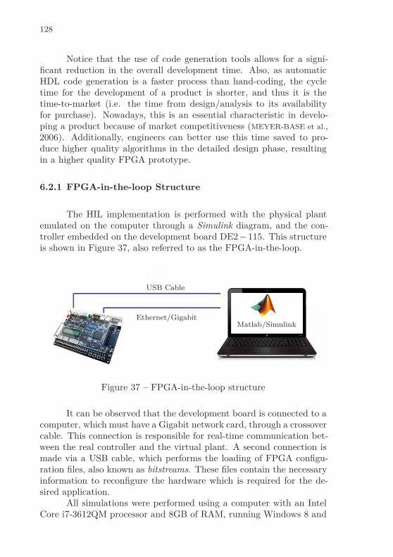
128
Notice that the use of code generation tools allows for a signi-ficant reduction in the overall development time. Also, as automaticHDL code generation is a faster process than hand-coding, the cycletime for the development of a product is shorter, and thus it is thetime-to-market (i.e. the time from design/analysis to its availabilityfor purchase). Nowadays, this is an essential characteristic in develo-ping a product because of market competitiveness (MEYER-BASE et al.,2006). Additionally, engineers can better use this time saved to pro-duce higher quality algorithms in the detailed design phase, resultingin a higher quality FPGA prototype.
6.2.1 FPGA-in-the-loop Structure
The HIL implementation is performed with the physical plantemulated on the computer through a Simulink diagram, and the con-troller embedded on the development board DE2 − 115. This structureis shown in Figure 37, also referred to as the FPGA-in-the-loop.
USB Cable
Ethernet/GigabitMatlab/Simulink
Figure 37 – FPGA-in-the-loop structure
It can be observed that the development board is connected to acomputer, which must have a Gigabit network card, through a crossovercable. This connection is responsible for real-time communication bet-ween the real controller and the virtual plant. A second connection ismade via a USB cable, which performs the loading of FPGA configu-ration files, also known as bitstreams. These files contain the necessaryinformation to reconfigure the hardware which is required for the de-sired application.
All simulations were performed using a computer with an IntelCore i7-3612QM processor and 8GB of RAM, running Windows 8 and
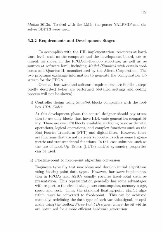
129
Matlab 2013a. To deal with the LMIs, the parser YALPMIP and thesolver SDPT3 were used.
6.2.2 Requirements and Development Stages
To accomplish with the HIL implementation, resources at hard-ware level, such as the computer and the development board, are re-quired, as shown in the FPGA-in-the-loop structure, as well as re-sources at software level, including Matlab/Simulink with certain tool-boxes and Quartus II, manufactured by the Altera Corporation. Thetwo programs exchange information to generate the configuration bit-stream for the FPGA.
Once all hardware and software requirements are fulfilled, stepsbriefly described below are performed (detailed settings and codingprocess will not be shown):
i) Controller design using Simulink blocks compatible with the tool-box HDL Coder
At this development phase the control designer should pay atten-tion to use only blocks that have HDL code generation compatibi-lity. There are over 170 blocks available, including basic arithmeticoperations, logical operations, and complex functions such as theFast Fourier Transform (FFT) and digital filter. However, thereare functions that are not natively supported, such as some trigono-metric and transcendental functions. In this case solutions such asthe use of Look-Up Tables (LUTs) and/or symmetry propertiescan be used.
ii) Floating-point to fixed-point algorithm conversion
Engineers typically test new ideas and develop initial algorithmsusing floating-point data types. However, hardware implementa-tion in FPGAs and ASICs usually requires fixed-point data re-presentation. This representation generally has some advantageswith respect to the circuit size, power consumption, memory usage,speed and cost. Thus, the standard floating-point Matlab algo-rithm must be converted to fixed-point. This can be achievedmanually, redefining the data type of each variable/signal, or opti-mally using the toolbox Fixed-Point Designer, where the bit widthsare optimized for a more efficient hardware generation.
130
iii) VHDL Coding
Once the controller algorithm is correctly set to run in fixed-point,the control designer have to generate the HDL code to be embed-ded in the FPGA development board. For this purpose the HDLcoder toolbox is employed, which can generate codes compatiblewith Simulink diagrams using the hardware description languagesVerilog and VHDL (or VHSIC hardware description language, fromVery High Speed Integrated Circuits). In this work the second lan-guage was used, which is currently the most popular.
iv) Preparing FPGA-in-the-loop simulation
In this step, the configurations for the proper communication bet-ween the virtual plant and the real controller are performed. ASimulink diagram should be built containing the dynamics of theplant, which will exchange data over the Ethernet network with thecontroller embedded in the development board DE2 − 115. Thus,for a correct communication between Simulink and developmentboard, the Internet Protocol (IP) settings must be correctly con-figured. To assist in this process, the HDL WorkAdvisor inside theHDL Coder toolbox can be used.
v) Loading FPGA and simulation
Finally, the code generated in the previous steps shall be loadedinto the FPGA by using an USB cable. Then, with the FPGAconfigured by the bitstream file, it is possible to execute the HILsimulation and analyze the collected data. Several reports are gene-rated, allowing comparisons in terms of time consumption, numberof operations, number of logic elements, among others, which areexplored in the example described in the following section.
6.2.3 Complexity of Implementation
The complexity analysis of the control systems digital implemen-tation is of great importance to determine the ideal programmable plat-form in which is embedded the control law, ensuring there exists enoughprocessing power to perform all the required computations in the stipu-lated time. In this perspective, together with the growing demand forhigh-performance devices with reduced size and low-energy consump-tion, the objective is to demonstrate that the use of N-fuzzy modelshas significant advantages, when compared to the classical fuzzy tech-niques.
131
It is worth noting that the fuzzy rule reduction provided by theuse of N-fuzzy models yields a smaller numerical complexity of thecontrol algorithms. This property has already been demonstrated inAppendix D, and it can also be checked considering the time requiredto solve the optimization problems of the preceding chapters. Thisis an important attribute because it prevents the computational bur-den from increasing to a point where solvers may fail even in solvingsimple problems. However, it should be clarified that, commonly, thecomputational system that solves the optimization algorithm is not thesame as that performing the control action. In addition, the processfor obtaining the controller gains runs offline, and it is not necessaryto recalculate at each sampling time. Thus, although there are obviousadvantages related to feasibility and the time to solve the control algo-rithms, the numerical complexity analysis has no direct influence overthe real implementation (platform to be chosen).
For comparing the complexity of implementation between con-trollers developed for classical and N-fuzzy models, the following dy-namic output feedback control laws are considered:
• Controller 1: Theorem 8.10 of Feng (2010)
• Controller 2: Theorem 1 of Klug, Castelan & Silva (2012)
The conditions established in the above articles have been adap-ted to obtain a fair comparative criterion. Hence, the conditions re-garding the domain of validity, saturation treatment, among others,were not taken into account. In other words, only those related to thestabilization problem were used.
6.2.3.1 Nonlinear System
Consider the unidimensional nonlinear system represented by:
x(k + 1) = x3(k) + sin(x(k)) + (0, 2 + x2(k))u(k). (6.1)
It is assumed, for instance, due to physical reasons, that the systemstate is restricted to the region represented by x(k) ∈ [−π/3, π/3].Therefore, it is possible to locally encompass the nonlinearity sin(xk)into a limited sector, i.e., ϕ(k) = sin(x(k)) ∈ S[Ω1, Ω2], with Ω1 =3√
3/2π and Ω2 = 1. Also, the premise variable νk = x2(k) is defined,and then ν(k) ∈ [d1, d2], with d1 = 0 and d2 = π2/9 being the limitsof ν(k). Thus, system (6.1) can be described by the following N-fuzzy
132
model with two nonlinear local rules:
x(k + 1) =2∑
i=1
α(i)(k) [dix(k) + (0, 2 + di)u(k)] + ϕ(k), (6.2)
with α(1)(k) =d2 − ν(k)
d2 − d1and α(2)(k) =
ν(k) − d1
d2 − d1.
Otherwise, the nonlinearity ϕ(k) might be rewritten as follows:
ϕ(k) = sin(x(k)) =
2∑
j=1
ǫ(j)(k)Ωj
x(k), (6.3)
with ǫ(j)(k), j = 1, 2, being any function validating (6.3) and satisfyingthe properties ǫ(1) + ǫ(2) = 1 and ǫ(j) ≥ 0, j = 1, 2. For instance, onecan choose1
ǫ(1) =
sin(x) − Ω1x
x(Ω2 − Ω1), x 6= 0
1, x = 0and ǫ(2) =
Ω2x − sin(x)
x(Ω2 − Ω1), x 6= 0
0, x = 0
Hence, the following classic T-S fuzzy model with four linear local rulesis obtained:
x(k + 1) =2∑
i=1
2∑
j=1
α(i)(k)ǫ(j)(k) (di + Ωj)x(k) + (0.2 + di)u(k)
=4∑
i=1
h(i)(k) Aix(k) + Biu(k)
(6.4)where Ai = di + Ωj , Bi = 0.2 + di and h(i)(k) = α(i)(k)ǫ(j)(k), fori = j + 2(i − 1) and i, j = 1, 2.
6.2.3.2 Results
Four different cases are defined to analyze the complexity of im-plementation, taking into account the type of fuzzy modeling used torepresent the system to be controlled and the structure of the dynamiccompensator (previously presented in section 6.2.3):
1For convenience, the time dependence is omitted.
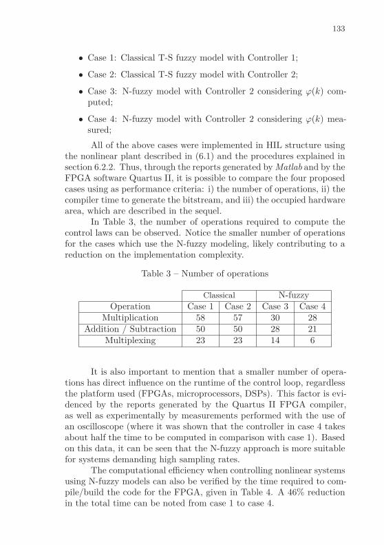
133
• Case 1: Classical T-S fuzzy model with Controller 1;
• Case 2: Classical T-S fuzzy model with Controller 2;
• Case 3: N-fuzzy model with Controller 2 considering ϕ(k) com-puted;
• Case 4: N-fuzzy model with Controller 2 considering ϕ(k) mea-sured;
All of the above cases were implemented in HIL structure usingthe nonlinear plant described in (6.1) and the procedures explained insection 6.2.2. Thus, through the reports generated by Matlab and by theFPGA software Quartus II, it is possible to compare the four proposedcases using as performance criteria: i) the number of operations, ii) thecompiler time to generate the bitstream, and iii) the occupied hardwarearea, which are described in the sequel.
In Table 3, the number of operations required to compute thecontrol laws can be observed. Notice the smaller number of operationsfor the cases which use the N-fuzzy modeling, likely contributing to areduction on the implementation complexity.
Table 3 – Number of operations
Classical N-fuzzyOperation Case 1 Case 2 Case 3 Case 4
Multiplication 58 57 30 28Addition / Subtraction 50 50 28 21
Multiplexing 23 23 14 6
It is also important to mention that a smaller number of opera-tions has direct influence on the runtime of the control loop, regardlessthe platform used (FPGAs, microprocessors, DSPs). This factor is evi-denced by the reports generated by the Quartus II FPGA compiler,as well as experimentally by measurements performed with the use ofan oscilloscope (where it was shown that the controller in case 4 takesabout half the time to be computed in comparison with case 1). Basedon this data, it can be seen that the N-fuzzy approach is more suitablefor systems demanding high sampling rates.
The computational efficiency when controlling nonlinear systemsusing N-fuzzy models can also be verified by the time required to com-pile/build the code for the FPGA, given in Table 4. A 46% reductionin the total time can be noted from case 1 to case 4.
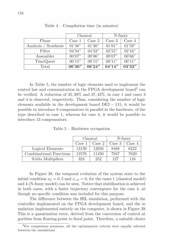
134
Table 4 – Compilation time (in minutes)
Classical N-fuzzyPhase Case 1 Case 2 Case 3 Case 4
Analysis / Synthesis 01’40” 01’30” 01’01” 01’59”Filter 04’34” 04’33” 02’55” 02’16”
Assembler 00’07” 00’06” 00’07” 00’06”TimeQuest 00’15” 00’15” 00’11” 00’11”
Total 06’36” 06’24” 04’14” 03’32”
In Table 5, the number of logic elements used to implement thecontrol law and communication in the FPGA development board2 canbe verified. A reduction of 35, 39% and 37, 42%, in case 1 and cases 3and 4 is observed, respectively. Thus, considering the number of logicelements available in the development board DE2 − 115, it would bepossible to introduce 8 compensators in parallel in the hardware, of thetype described in case 1, whereas for case 4, it would be possible tointroduce 13 compensators.
Table 5 – Hardware occupation
Classical N-fuzzyCase 1 Case 2 Case 3 Case 4
Logical Elements 13139 12056 8488 8222Combinational Functions 12576 11450 7947 7620
9-bits Multipliers 324 252 127 116
In Figure 38, the temporal evolution of the system state to theinitial condition x0 = 0, 5 and xc,0 = 0, for the cases 1 (classical model)and 4 (N-fuzzy model) can be seen. Notice that stabilization is achievedin both cases, with a faster trajectory convergence for the case 4, al-though no specific condition was included for this purpose.
The difference between the HIL simulation, performed with thecontroller implemented on the FPGA development board, and the si-mulation implemented entirely on the computer, is shown in Figure 39.This is a quantization error, derived from the conversion of control al-gorithm from floating-point to fixed point. Therefore, a suitable choice
2For comparison purposes, all the optimization criteria were equally selectedbetween the simulations
135
0 1 2 3 4 5 6 7 8 9 100
0.1
0.2
0.3
0.4
0.5
0.6
0.7
k(samples)
xk
case 1case 4
Figure 38 – State trajectory x(k)
of the bit widths is important to avoid overflows, which may affect theperformance of the closed loop system.
0 1 2 3 4 5 6 7 8 9 100
0.5
1
1.5
2
2.5
3
3.5
4x 10
−3
k(samples)
Err
or
case 1case 4
Figure 39 – Quantization error
6.3 CONCLUDING REMARKS
In this chapter, general tools concerning the analysis and designof nonlinear control systems using T-S fuzzy models were presented.Two software programs were developed in order to assist researchersand engineers to design, in a few steps, a reasonable controller for aknown nonlinear system. It also allows users to quickly obtain resultsfor comparison with their own techniques. From another point of view,the software interactivity enhances the learning process by exploiting
136
the advantages of immediately seeing the effects of changes, which cannever be shown in static pictures. Three languages are available, as wellas other interesting features, such as different types of modeling, pre-defined examples, possibility to open/save and export data in variousformats, as well as the execution of open and closed-loop simulations.Presently, the first app has been published as a Matlab app, also runningfrom an executable file, provided the user has the Matlab CompilerRuntime (MCR) installed. In a future release it will be launched it as astandalone application, independent of external libraries and/or othertoolboxes.
Regarding the practical implementation of fuzzy controllers, HILsimulations were performed considering the physical plant running vir-tually in a Matlab/Simulink environment using a desktop computer,and the control law embedded in a FPGA development board. Thus,a higher numerical and implementation efficiency when using N-fuzzymodels was demonstrated, with a significant reduction in the computa-tional burden required to obtain the controller gains, in the time takento generate the internal architecture of the FPGA, in the number ofoperations to compute the control law, and in the area of the FPGA cir-cuit. This proves that the use of the N-fuzzy model is more adequate forcritical applications in terms of sampling rate, and/or low-powered pro-gramming platforms, without compromising the overall performance ofthe control system.
7 CONCLUSION
In this thesis, novel approaches to control design, applied tononlinear discrete-time systems by means of T-S fuzzy models havebeen presented. For fuzzy modeling, an alternative method was pro-posed based on the use of nonlinear local rules, instead of the classicalones, providing the following benefits: i) it can reduce the number ofrules when compared to the classical T-S representation, leading toa lower numerical complexity while maintaining the model exactness;and ii) it allows the design and practical implementation of dynamicoutput feedback controllers in the presence of unmeasurable nonlineari-ties. Furthermore, the proposed results consider inherent issues in thecontrol problem, such as the regional validity of the T-S fuzzy models,physical constraints of actuators, and the presence of external signalsusually found in real systems. Examples were provided throughout thedocument, in order to illustrate the proposed techniques.
At first, in Chapter 2, the features and mathematical machineryof T-S fuzzy models were presented. The procedure to obtain an N-fuzzy model for a class of nonlinear systems was described in detail. Itis important to remark that the local characteristic of T-S modeling isoften not considered in most literature FMB results, which may lead topoor performance or even instability of the closed-loop system. Also,rule reduction, provided by the use of nonlinear local submodels, and itsimplication in the numerical complexity, were demonstrated, preventingthe computational burden from increasing to a point where solvers mayfail to solve even simple problems.
Next, in Chapter 3, the synthesis of a fuzzy dynamic outputfeedback controller was discussed, taking into account the saturationof the actuator and the regional validity of the fuzzy model. An anti-windup gain was considered as an attempt to mitigate the undesiredeffects of saturation, as well as the use of a performance index basedon the λ-contractivity of the level set, associated with the Lyapunovfunction, in order to ensure a certain rate of temporal convergence ofthe closed-loop system trajectories.
In Chapters 4 and 5, the control of nonlinear systems subject toexternal disturbances, bounded in energy and amplitude, respectively,was considered. In the first case, LMI-based conditions and three con-vex optimization problems were proposed to locally ensure the input-to-state stability in the ℓ2-sense and a certain input-to-output performancethrough an upper bound for the system ℓ2-gain. Otherwise, in the pre-

138
sence of amplitude bounded disturbances, it is not possible to ensurethe asymptotic stability of the origin, and in this case the concept ofultimate bounded (UB) stability was considered. Two ellipsoidal setshaving different shapes, associated to the set of admissible initial con-ditions and to the concept of UB stability, were taken into accountto handle the control problem. Moreover, the proposed dynamic con-troller admits the presence of unmeasurable nonlinearities, which is notpossible for the classical PDC dynamic controllers.
Later, in Chapter 6, practical aspects of the real implementationof fuzzy controllers were considered. Hardware-in-the-loop simulationswere performed, enabling the complexity analysis of the digital imple-mentation of classical and N-fuzzy controllers. Also, an interactive toolaiming to assist students and researchers in the nonlinear control designusing fuzzy strategies was presented.
7.1 CONTRIBUTIONS OF THE THESIS
Prior to this document, the contributions of the research through-out this PhD include the following journal articles:
• Local Stabilization of Nonlinear Discrete-Time SystemsSubject to Amplitude Bounded Disturbances. Klug, M.,Castelan, E. B. and Coutinho, D. in submission process.
• T-S Fuzzy Approach to the Local Stabilization of Nonli-near Discrete-Time Systems Subject to Energy-BoundedDisturbances. Klug, M., Castelan, E. B. and Coutinho, D.Journal of Control, Automation and Electrical Systems - IJCAES2015.
• Fuzzy Dynamic Output Feedback Control Through Non-linear Takagi-Sugeno Models. Klug, M., Castelan, E. B.,Leite, V. J. S. and Silva, L. F. P. Fuzzy Sets and Systems - FSS2014.
• Local Stabilization of Time-Delay Nonlinear Discrete-TimeSystems Using Takagi-Sugeno Models and Convex Opti-mization. Silva, L. F. P., Leite, V. J. S., Castelan, E. B. andKlug, M. Mathematical Problems in Engineering - 2014.
• Compensadores Dinâmicos para Sistemas Discretos noTempo com Parâmetros Variantes e Aplicação a um Sis-

139
tema Fuzzy Takagi-Sugeno. Klug, M. and Castelan, E. B.Revista SBA: Controle & Automação - 2012.
The following papers, published in conference proceedings, were also apart of this research:
• Interactive Software for Modeling and Control of Nonli-near Systems: A T-S Fuzzy Approach. Klug, M., Castelan,E. B. and Coutinho, D. XII Simpósio Brasileiro de AutomaçãoInteligente - SBAI 2015.
• Compensadores Dinâmicos para Sistemas Não LinearesUtilizando Modelos Fuzzy T-S: Estudo Comparativo eImplementação HIL. Klug, M., Castelan, E. B., Coutinho, D.and Silva, L. F. P. XX Congresso Brasileiro de Automática - CBA2014.
• Local Stabilization of Nonlinear Discrete-Time Systemswith Uncertain Time-Delay Using T-S Models. Silva, L.F. P., Leite, V. J. S., Castelan, E. B., Feng, G. and Klug, M. XXCongresso Brasileiro de Automática - CBA 2014.
• Control of Nonlinear Discrete-Time Systems Subject toℓ2-Bounded Disturbances Using Local Nonlinear FuzzyT-S Models. Klug, M., Castelan, E. B. and Coutinho, D. IEEE52nd Annual Conference on Decision and Control - CDC 2013.
• Controle Seguro de Sistemas Não Lineares UtilizandoModelos Híbridos Fuzzy L’ure com Saturação dos At-uadores. Klug, M., Castelan, E. B. and Silva, L. F. P. XIXCongresso Brasileiro de Automática - CBA 2012.
• Síntese Convexa de Controladores Fuzzy para SistemasTakagi-Sugeno Discretos no Tempo com Atraso e Limi-tação nos Estados. Silva, L. F. P., Leite, V. J. S., Castelan, E.B. and Klug, M. XIX Congresso Brasileiro de Automática - CBA2012.
• A Dynamic Compensator for Parameter Varying Sys-tems Subject to Actuator Limitations Applied to a T-SFuzzy System. Klug, M., Castelan, E. B. and Leite, V. J. S.Proc. of 18th IFAC World Congress - IFAC 2011.
• Redução de Regras e Compensação Robusta para Sis-temas Takagi-Sugeno com Utilização de Modelos Não

140
Lineares Locais. Klug, M. and Castelan, E. B. X SimpósioBrasileiro de Automação Inteligente - SBAI 2011.
Further, all acquired expertise also provided the doctoral studentwith the opportunity to give a lecture entitled “Control of NonlinearSystems Using T-S Fuzzy Models: Theory and Implementation”, of-fered in CBA 2014, as well as invitations to review articles in the follo-wing journals: Automatica, Journal of the Franklin Institute, Mathe-matical Problems in Engineering, IET Control Theory & Applications,International Journal of Adaptative Control and Signal Processing andNeurocomputing; and conferences: IFAC 2011, CBA 2012 and 2014,SBAI 2011 and 2015, and ISIE 2015.
7.2 PERSPECTIVES
Among some possible extensions to the work presented in thisthesis, the following research directions can be mentioned:
• Extend the proposed approaches to the application in nonlinearcontinuous-time systems;
• Investigate the use of N-fuzzy models with non-PDC strategies,suitable for static and dynamic output feedback controllers;
• Consider other typical actuator nonlinearities, such as dead-zone,backlash, hysteresis and relay;
• Analyze the effects of discretization when considering hybrid sys-tems;
• Improve the control algorithms in order to obtain less conservativeresults regarding the guaranteed domain of stability;
• Apply the concepts and strategies developed to real systems.
141
REFERENCES
ALATA, M.; DEMIRLI, K.; BULGAK, A. Interpolation behaviorof T-S fuzzy controllers. In: IEEE International Symposium onIntelligent Control. Cambridge, MA, USA: [s.n.], 1999. p. 359–364.
ANDREA, C. Q.; PINTO, J. O. P.; ASSUNÇÃO, E.; TEIXEIRA, M.C. M. Controle ótimo H∞ de sistemas não lineares com modelos fuzzyTakagi-Sugeno. Revista Controle & Automação, v. 19, n. 3, p. 256–269,2008.
ARCAK, M.; LARSEN, M.; KOKOTOVIC, P. Circle and Popovcriteria as tools for nonlinear feedback designs. Automatica, v. 39, p.643–650, 2003.
ASEMANI, M. H.; MAJD, V. J. A robust H∞ observer-basedcontroller design for uncertain T–S fuzzy systems with unknownpremise variables via LMI. Fuzzy Sets and Systems, v. 212, n. 1, p.21–40, 2013.
BEEK, S.; SHARMA, S. Best practices for FPGA prototyping ofMatlab and Simulink algotithms. Journal of Electronic Engineering,2011.
BOYD, S.; GHAOUI, L. E.; FERON, E.; BALAKRISHNAN, V.Linear Matrix Inequalities in System and Control Theory. Philadelphia,USA: Society for Industrial and Applied Mathematics, 1994.
CASTELAN, E. B.; LEITE, V. J. S.; MIRANDA, M. F.; MORAES,V. M. Synthesis of Output Feedback Controllers for a Class ofNonlinear Parameter-Varying Discrete-Time Systems Subject toActuators Limitations. In: American Control Conference (ACC), 2010.Baltimore, USA: [s.n.], 2010. p. 4235–4240.
CASTELAN, E. B.; TARBOURIECH, S.; QUEINNEC, I. Controldesign for a class of nonlinear continuous-time systems. Automatica,v. 44, n. 8, p. 2034–2039, 2008.
CHADLI, M.; GUERRA, T. M. LMI Solution for Robust StaticOutput Feedback Control of Takagi-Sugeno Fuzzy Models. IEEETransactions on Fuzzy Systems, v. 20, n. 6, p. 1160–1165, 2012.
142
CHANG, X. Robust nonfragile H∞ filter of fuzzy systems with linearfractional parametric uncertainties. IEEE Transactions on FuzzySystems, v. 20, n. 6, p. 1001–1011, 2012.
CHANG, X.; YANG, G. Nonfragile H∞ filter desing for T-Sfuzzy systems in standard form. IEEE Transactions on IndustrialElectronics, v. 61, n. 7, p. 3448–3458, 2014.
DARUICHI, E. R. M. Modelagem e Controle de Sistemas FuzzyTakagi-Sugeno. Tese (Doutorado) — Universidade Estadual Paulista(UNESP) - Faculdade de Engenharia de Ilha Solteira, 2003.
DILDA, V.; JUNGERS, M.; CASTELAN, E. B. Uniform ultimateboundedness analysis and synthesis for linear systems with dead-zonein the actuators. International Journal of Robust and NonlinearControl, doi:10.1002/rnc.3223, 2014.
DONG, J.; WANG, Y.; YANG, G. Control synthesis of continuous-time T-S fuzzy systems with local nonlinear models. Systems, Man,and Cybernetics, Part B: Cybernetics, IEEE Transactions on, v. 39,n. 5, p. 1245–1258, October 2009.
DONG, J.; WANG, Y.; YANG, G. Output feedback fuzzy controllerdesign with local nonlinear feedback laws for discrete-time nonlinearsystems. Systems, Man, and Cybernetics, Part B: Cybernetics, IEEETransactions on, v. 40, n. 6, p. 1447–1459, December 2010.
DONG, J.; YANG, G. Dynamic output feedback control synthesisfor continuous-time T-S fuzzy systems via a switched fuzzy controlscheme. Systems, Man, and Cybernetics, Part B: Cybernetics, IEEETransactions on, v. 38, n. 4, p. 1166–1175, August 2008.
FARIA, F. A.; SILVA, G. N.; OLIVEIRA, V. A. Reducing theconservatism of LMI-based stabilization conditions for T-S fuzzysystems using fuzzy Lyapunov functions. International Journal ofSystems Science, v. 44, n. 10, p. 1956–1969, 2013.
FENG, G. A survey on analysis and design of model-based fuzzycontrol systems. Fuzzy Systems, IEEE Transactions on, v. 14, n. 5, p.676–697, October 2006.
FENG, G. Analysis and Synthesis of Fuzzy Control Systems: AModel-Based Approach. [S.l.]: CRC Press, 2010.

143
FENG, G.; MA, J. Quadratic stabilization of uncertain discrete-timefuzzy dynamics systems. IEEE Transaction on Circuits and Systems -I: Fundamental Theory and Applications, v. 48, n. 11, p. 1337–1344,2001.
FIGUEREDO, L. F. C.; ISHIHARA, J. Y.; BORGES, G. A.;BAUCHSPIESS, A. Robust H∞ output tracking control for a class ofnonlinear systems with time-varying delays. Circuits, Systems andSignal Processing, v. 33, p. 1451–1471, 2014.
GAHINET, P.; NEMIROVSKI, A.; LAUB, A. J.; CHILALI, M. LMIControl Toolbox for use with Matlab - User Guide. Natick, MA: TheMathWorks Inc, 1995.
GAO, Q.; ZENG, X. J.; FENG, G.; WANG, Y. Universal FuzzyModels and Universal Fuzzy Controllers Based on GeneralizedT-S Fuzzy Models. In: IEEE World Congress on ComputationalIntelligence, Brisbane, Australia. [S.l.: s.n.], 2012.
GOLABI, A.; BEHESHTI, M.; ASEMANI, M. H. H∞ robust fuzzydynamic observer-based controller for uncertain Takagi-Sugenofuzzy systems. IET Control Theory and Applications, v. 6, n. 10, p.1434–1444, 2012.
Gomes da Silva Jr., J. M.; TARBOURIECH, S. Anti-windupdesign with guaranteed regions of stability: an LMI-based approach.Automatic Control, IEEE Transactions on, v. 50, n. 1, p. 106–111,January 2005.
GUERRA, T. M.; BERNAL, M.; GUELTON, K.; LABIOD, S. Non-Quadratic Local Stabilization for Continuous-Time Takagi-SugenoModels. Fuzzy Sets and Systems, v. 201, n. 16, p. 40–54, 2012.
GUERRA, T. M.; KERKENI, H.; LAUBER, J.; VERMEIREN, L. Anefficient Lyapunov function for discrete T-S models: Observer design.IEEE Transactions on Fuzzy Systems, v. 20, n. 1, p. 187–192, 2012.
GUERRA, T.-M.; KRUSZEWSKI, A.; LAUBER, J. DiscreteTagaki-Sugeno models for control: Where are we? Annual Reviews inControl, v. 33, n. 1, p. 37–47, 2009.
GUERRA, T. M.; VERMEIREN, L. LMI-based relaxed nonquadraticstabilization conditions for nonlinear systems in the Takagi-Sugeno’sform. Automatica, v. 40, n. 5, p. 823–829, 2004.

144
GUPTA, V.; KHARE, K.; SINGH, R. P. Efficient Design andFPGA Implementation of Digital Controller Using Xilinx SysGen.International Journal of Electronics Engineering, v. 2, n. 1, p. 99–102,2010.
GUZMAN, J. L.; ASTRON, K. J.; DORMIDO, S.; HAGGLUND, T.;PIGUET, Y.; BERENGUEL, M. Interactive learning module: Basicmodelling and identification concepts. In: Proceedings of the 17thIFAC World Congress. [S.l.: s.n.], 2008. p. 14606–14611.
HU, T.; Z., L. Composite quadratic Lyapunov functions for contrainedcontrol systems. Automatic Control, IEEE Transactions on, v. 48,n. 3, p. 440–450, March 2003.
HU, T.; Z., L.; M., C. B. An analysis and design method for linearsystems subject to actuator saturation and disturbance. Automatica,v. 38, n. 2, p. 351–359, 2002.
HUANG, S.; HE, X.; ZHANG, N. New results on H∞ filter designfor nonlinear systems with time delay via T-S fuzzy models. IEEETransactions on Fuzzy Systems, v. 19, n. 1, p. 193–199, 2011.
JUNGERS, M.; CASTELAN, E. Gain-sheduled control design for aclass of discrete-time nonlinear systems with saturating actuators.Systems & Control Letters, v. 60, n. 3, p. 169–173, 2011.
KHALIL, H. K. Nonlinear Systems. Third. [S.l.]: Prentice Hall, 2003.
KLUG, M.; CASTELAN, E.; COUTINHO, D. Local stabilizationof nonlinear discrete-time systems subject to amplitude boundeddisturbances. Submitted to the International Journal of SystemsScience, 2015.
KLUG, M.; CASTELAN, E.; SILVA, L. F. P. Controle seguro desistemas não lineares utilizando modelos híbridos Fuzzy L’ure comsaturação nos atuadores. In: Proc. of XIX CBA. [S.l.: s.n.], 2012. p.2620–2626.
KLUG, M.; CASTELAN, E. B. Redução de regras e compensaçãorobusta para sistemas Takagi-Sugeno com utilização de modelos nãolineares locais. In: Proc. of X SBAI. [S.l.: s.n.], 2011.
KLUG, M.; CASTELAN, E. B. Compensadores dinâmicos parasistemas discretos no tempo com parâmetros variantes e aplicaçãoa um sistema fuzzy Takagi-Sugeno. Revista Controle & Automação,v. 23, n. 5, p. 517–529, 2012.
145
KLUG, M.; CASTELAN, E. B.; COUTINHO, D. Control of nonlineardiscrete-time systems subject to ℓ2-bounded disturbances using localnonlinear fuzzy T-S models. In: 52nd IEEE Conference on Decisionand Control. [S.l.: s.n.], 2013.
KLUG, M.; CASTELAN, E. B.; COUTINHO, D. Interactive Softwarefor Modeling and Control of Nonlinear Systems: A T-S FuzzyApproach. In: Proc. of XII SBAI. [S.l.: s.n.], 2015.
KLUG, M.; CASTELAN, E. B.; COUTINHO, D. A T-S fuzzyapproach to the local stabilization of nonlinear discrete-timesystems subject to energy-bounded disturbances. Journal of Control,Automation and Electrical Systems, v. 26, n. 3, p. 191–200, 2015.
KLUG, M.; CASTELAN, E. B.; COUTINHO, D.; SILVA, L. F. P.Compensadores Dinâmicos para Sistemas Não Lineares UtilizandoModelos Fuzzy T-S: Estudo Comparativo e Implementação HIL. In:Proc. of XX CBA. [S.l.: s.n.], 2014.
KLUG, M.; CASTELAN, E. B.; LEITE, V. J. S. A dynamiccompensator for parameter varying systems subject to actuatorlimitations applied to a T-S fuzzy system. In: Proc. of 18th IFACWorld Congress. Milan, Italy: [s.n.], 2011. p. 14495–14500.
KLUG, M.; CASTELAN, E. B.; LEITE, V. J. S.; SILVA, L.F. P. Fuzzy dynamic output feedback control through nonlinearTakagi-Sugeno models. Fuzzy Sets and Systems, v. 263, p. 92–111,2014.
KOSKO, B. Fuzzy Engineering. [S.l.]: Prentice Hall, 1997.
LAM, H. K. LMI-based stability analysis for fuzzy-model-basedcontrol systems using artificial T-S fuzzy model. IEEE Transactionson Fuzzy Systems, v. 19, n. 3, p. 505–513, 2011.
LEE, D. H.; JOO, Y. H.; TAK, M. H. Local H∞ Control andInvariant Set Analysis for Continuous-Time T–S Fuzzy Systems withMagnitude- and Energy-Bounded Disturbances. In: Proc. of IEEEInternational Conference on Fuzzy Systems. Beijing, China: [s.n.],2014. p. 1990–1997.
LEEKWIJCK W. V. AMD KERRE, E. Defuzzification: Criteria andclassification. Fuzzy Sets and Systems, v. 108, n. 2, p. 159–178, 1999.
146
LEITE, V. J. S.; MONTAGNER, V. F.; OLIVEIRA, P. J.; OLIVEIRA,R. C. L. F.; RAMOS, D. C. W.; PERES, P. L. D. Estabilidade robustade sistemas lineares através de desigualdades matriciais lineares.Revista Controle & Automação, SciELO Brasil, v. 15, p. 24–40, 2004.
LöFBERG, J. YALMIP: A toolbox for modeling and optimization inMATLAB. In: Proceedings of the CACSD Conference. Taipei, Taiwan:[s.n.], 2004.
LI, F.; SHI, P.; WU, L.; ZHANG, X. Fuzzy-Model-Based D-Stabilityand Nonfragile Control for Discrete-Time Descriptor Systems WithMultiple Delays. IEEE Transactions on Fuzzy Systems, v. 22, n. 4,2014.
LIBERZON, M. R. Essays on the absolute stability theory. Automationand Remote Control, v. 67, n. 10, p. 1610–1644, 2006.
LO, J. C.; LIN, M. L. Robust H∞ nonlinear control via fuzzy staticoutput feedback. IEEE Transactions on Circuits and Systems I:Fundamental Theory and Applications, v. 50, n. 11, p. 1494–1502,2003.
LOPES, A. B.; FAVARIM, F.; CARATI, E. G. Estruturas ParalelasBaseadas em FPGA para Implementação de Compensadores Seletivosde Harmônicas. In: Proc. of XX CBAI. [S.l.: s.n.], 2012. p. 3329–3336.
MAMDANI, E. Application of fuzzy algotithms for control of simpledynamic plant. In: IEEE Control & Science. [S.l.: s.n.], 1974. v. 121,n. 12, p. 1585–1588.
MAMDANI, E. Application of Fuzzy Logic to Approximate ReasoningUsing Linguistic Synthesis. IEEE Transactions on Computers, v. 26,n. 12, p. 1182–1191, 1977.
MAMDANI, E. H.; ASSILIAN, S. An experiment in linguisticsynthesis with a fuzzy logic controller. Int. J. Man-machine Studies,v. 7, p. 1–13, 1975.
MEYER-BASE, U.; VERA, A.; MEYER-BASE, A.; PATTICHIS,M.; PERRY, R. Discrete Wavelet Transform FPGA Design UsingMatlab/Simulink. In: Proc. of International Society for Optics andPhotonics. [S.l.: s.n.], 2006. v. 6247.
MONTAGNER, V. F.; OLIVEIRA, R. C.; PERES, P. L. D.Relaxações convexas de convergência garantida para o projeto de
147
controladores para sistemas nebulosos de Takagi Sugeno. RevistaControle & Automação, v. 21, n. 1, p. 82–95, 2010.
MOZELLI, L. A.; PALHARES, R. M. Less conservative H∞ fuzzycontrol for discrete-time Takagi-Sugeno systems. MathematicalProblems in Engineering, 2011.
MOZELLI, L. A.; PALHARES, R. M. Stability analysis of lineartime-varying systems: improving conditions by adding moreinformation about parameter variation. Systems & Control Letters,v. 60, n. 5, p. 338–343, 2011.
NGUYEN, A.; DEQUIDT, A.; DAMBRINE, M. Anti-windupbased dynamic output feedback controller design with performanceconsideration for constrained Takagi-Sugeno systems. EngineeringApplications of Artificial Intelligence, v. 40, p. 76–83, 2015.
OLIVEIRA, M. Z.; SILVA JUNIOR, J. M. G.; COUTINHO, D.;TARBOURIECH, S. Anti-windup Design for a Class of MultivariableNonlinear Control Systems: an LMI-based Approach. In: 50th IEEEConference on Decision and Control, 2011. CDC. [S.l.: s.n.], 2011. p.4797–4802.
QIU, J.; FENG, G.; GAO, H. Static-output-feedback H∞ controlof continous-time T-S fuzzy affine systems via piecewise Lyapunovfunctions. IEEE Transactions on Fuzzy Systems, v. 21, n. 2, p.245–261, 2013.
SCHERER, C.; GAHINET, P.; CHILALI, M. Multiobjectiveoutput-feedback control via LMI optimization. Automatic Control,IEEE Transactions on, v. 42, n. 7, p. 896–911, July 1997.
SILVA, L. F. P.; LEITE, V. J. S.; CASTELAN, E. B.; KLUG, M.Local Stabilization of Time-Delay Nonlinear Discrete-Time SystemsUsing Takagi-Sugeno Models and Convex Optimization. MathematicalProblems in Engineering, v. 2014, n. 10 pages, 2014.
STURM, J. Using SeDuMi 1.02, a MATLAB toolbox for optimizationover symmetric cones. Optimization Methods and Software, v. 11-12,p. 625–653, 1999.
SU, X.; SHI, P.; WU, L.; SONG, Y. A novel approach to filter designfor T-S fuzzzy discrete-time systems with time-varying delay. IEEETransactions on Fuzzy Systems, v. 20, n. 6, p. 1114–1129, 2012.

148
TAKAGI, T.; SUGENO, M. Fuzzy identification of systems and itsapplications to modeling and control. IEEE Transactions on Systems,Man and Cybernetics, SMC-15, n. 1, p. 116–132, 1985.
TANAKA, K.; TANAKA, M.; OHTAKE, H.; WANG, H. O.Polynomial fuzzy observer designs: A sum-of-squares approach. IEEETransactions on Systems, Man, and Cybernetics, v. 42, n. 5, p.1330–1342, 2012.
TANAKA, K.; TANAKA, M.; OHTAKE, H.; WANG, H. O. Sharednonlinear control in wireless-based remote stabilization: A theoreticalapproach. IEEE/ASME Transactions on Mechatronics, v. 17, n. 3, p.443–453, 2012.
TANAKA, K.; WANG, H. O. Fuzzy Control Systems Design andAnalysis: A Linear Matrix Inequality Approach. New York, USA: JohnWiley & Sons, 2001.
TANIGUCHI, T.; TANAKA, K.; OHTAKE, H.; WANG, H. O. Modelconstruction, rule reduction, and robust compensation for generalizedform of Takagi-Sugeno fuzzy systems. IEEE Transactions on FuzzySystems, v. 9, n. 4, p. 525–538, August 2001.
TARBOURIECH, S.; GARCIA, G.; Gomes da Silva Jr., J. M.;QUEINNEC, I. Stability and Stabilization of Linear Systems withSaturating Actuators. [S.l.]: Springer-Verlag London, 2011.
TARBOURIECH, S.; QUEINNEC, I.; ALAMO, T.; FIACCHINI,M.; CAMACHO, T. Ultimate bounded stability and stabilization oflinear systems interconnected with generalized saturated functions.Automatica, v. 47, n. 1, p. 1473–1481, 2011.
TARBOURIECH, S.; VALMÓRBIDA, G.; GARCIA, G.; BIANNIC,J.-M. Stability and performance analysis for linear systems withactuator and sensor saturations subject to unmodeled dynamics. In:Proceedings of the 2008 American Control Conference. Seattle, WA,USA: [s.n.], 2008. p. 401–406.
TEIXEIRA, M. C. M.; ZAK, H. Stabilizing controller design foruncertains nonlinear systems using fuzzy models. IEEE Transactionson Fuzzy Systems, v. 7, n. 2, p. 133–142, 1999.
TOGNETTI, E. S.; OLIVEIRA, R. C. L. F.; PERES, P. L. D.Selective H2 and H∞ stabilization of Takagi-Sugeno fuzzy systems.IEEE Transactions on Fuzzy Systems, v. 19, n. 5, p. 890–900, 2011.

149
TOGNETTI, E. S.; OLIVEIRA, R. C. L. F.; PERES, P. L. D.Reduced-order dynamic output feedback control of continuou-timeT-S fuzzy systems. Fuzzy Sets and Systems, v. 207, p. 27–44, 2012.
TOGNETTI, E. S.; OLIVEIRA, R. C. L. F.; PERES, P. L. D. LMIRelaxations for H∞ and H2 Static Output Feedback of Takagi-SugenoContinuous-Time Fuzzy Systems. Journal of Control, Automation andElectrical Systems, v. 24, p. 33–45, 2013.
TOGNETTI, E. S.; OLIVEIRA, V. A. Fuzzy pole placement based onpiecewise Lyapunov functions. International Journal of Robust andNonlinear Control, v. 20, p. 571–578, 2009.
TOH, K. C.; TUTUNCU, R. H.; TODD, M. J. On the implementationof SDPT3 (version 3.1) - a MATLAB software package forSemidefinite-Quadratic-Linear Programming. In: IEEE InternationalSymposium on CACSD. [S.l.: s.n.], 2004. p. 290–296.
VIDYASAGAR, M. Nonlinear Systems Analysis. Second. [S.l.]: SIAM:Society for Industrial and Applied Mathematics, 2002.
WANG, L. K.; LIU, X. D. Local analysis of continuous-timeTakagi–Sugeno fuzzy system with disturbances bounded by magnitudeor energy: A Lagrange multiplier method. Information Sciences,v. 248, n. 1, p. 89–102, 2013.
WANG, L. K.; PENG, J. L.; LIU, X. D.; ZHANG, H. G. An approachto observer design of continuous-time Takagi–Sugeno fuzzy modelwith bounded disturbances. Information Sciences, v. 324, n. 1, p.108–125, 2015.
WU, L.; SU, X.; SHI, P.; QIU, J. A new approach to stabilityanalysis and stabilization of discrete-time T-S fuzzy time-varyingdelay systems. IEEE Transactions on Systems Man and Cybernetics,v. 41, n. 1, p. 273–286, 2011.
YANG, Z.; YANG, Y. New delay-dependent stability analysis andsynthesis of T-S fuzzy systems with time-varying delay. InternationalJournal of Robust and Nonlinear Control, v. 20, p. 313–322, 2012.
YONEYAMA, J. Non-fragile output feedback control design ofuncertain Takagi-Sugeno fuzzy systems. In: 53rd IEEE Conference onDecision and Control. [S.l.: s.n.], 2014. p. 6764–6769.

150
ZADEH, L. Fuzzy sets. Information and Control, v. 8, p. 338–353,1965.
ZHANG, K.; JIANG, B.; STAROSWIECKI, M. Dynamic outputfeedbacl fault tolerant controller design for Takagi-Sugeno fuzzysystems with actuators faults. IEEE Transactions on Fuzzy Systems,v. 18, n. 1, p. 194–201, 2010.
ZHU, B.; LIU, A.; GU, Y.; ZHANG, Q. Finite-time H∞ performanceanalysis for a kind of T-S fuzzy descriptor system with time-Delayelay.In: 27th CCDC. [S.l.: s.n.], 2015. p. 210–215.

APPENDIX A -- Approximate Modeling

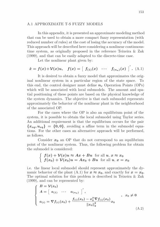
153
A.1 APPROXIMATE T-S FUZZY MODELS
In this appendix, it is presented an approximate modeling methodthat can be used to obtain a more compact fuzzy representation (withreduced number of rules) at the cost of losing the accuracy of the model.This approach will be described here considering a nonlinear continuous-time system, as originally proposed in the reference Teixeira & Zak(1999), and that can be easily adapted to the discrete-time case.
Let the nonlinear plant given by:
x = f(x)+V(x)u, f(x) =[
f(1)(x) · · · f(nx)(x)]
′
. (A.1)
It is desired to obtain a fuzzy model that approximates the orig-inal nonlinear system in a particular region of the state space. Tothis end, the control designer must define nr Operation Points (OPs)which will be associated with local submodels. The amount and spa-tial positioning of these points are based on the physical knowledge ofthe system dynamics. The objective is that each submodel representsapproximately the behavior of the nonlinear plant in the neighborhoodof the associated OP.
For the cases where the OP is also an equilibrium point of thesystem, it is possible to obtain the local submodel using Taylor series.An additional requirement is that the equilibrium occurs for the pairxeq, ueq = 0, 0, avoiding a affine term in the submodel equa-tions. For the other cases an alternative approach will be performed,as follows.
Consider x0 an OP that do not correspond to an equilibriumpoint of the nonlinear system. Thus, the following problem for obtainthe submodel is considered:
f(x) + V(x)u ≈ Ax + Bu for all u, x ≈ x0
f(x0) + V(x0)u = Ax0 + Bu for all u, x = x0
i.e. the linear local submodel should represent approximately the dy-namic behavior of the plant (A.1) for x ≈ x0, and exactly for x = x0.The optimal solution for this problem is described in Teixeira & Zak(1999), and can be represented by:
B = V(x0)
A =[
a(1) · · · a(nx)
]′
,
a(i) = ∇f(i)(x0) +f(i)(x0) − xT
0 ∇f(i)(x0)
‖x0‖22
x0
, x0 6= 0
(A.2)

154
where ∇f(i)(x) =[
∂f(i)(x)/∂x(1) · · · ∂f(i)(x)/∂x(nx)
]′
and‖x0‖
2 = x′
0x0. So, the T-S fuzzy model is given by
x =nr∑
i=1
h(i) Aix + Biu
with h(i), ∀ i = 1, ..nr being membership functions chosen by thecontrol designer generally with one of the following shapes: triangular,trapezoidal, gaussian or bell, as show in Figure 40.
(a) Triangular (b) Trapezoidal
(c) Gaussian (d) Bell
Figure 40 – Typical membership functions
It is interesting to emphasize again, that the optimal local mo-dels, for OPs that are not equilibrium points of the systems, cannotbe obtained by linearization using Taylor series. This is due to thefact that Taylor linearizes the model in terms of the variations of thevariables, and not in their original values, thus yielding an affine modelfor each OP that is not an equilibrium point.
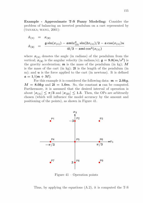
155
Example - Approximate T-S Fuzzy Modeling: Consider theproblem of balancing an inverted pendulum on a cart represented by(TANAKA; WANG, 2001):
x(1) = x(2)
x(2) =g sin(x(1)) − amlx2
(2) sin(2x(1))/2 − a cos(x(1))u
4l/3 − aml cos2(x(1))
where x(1) denotes the angle (in radians) of the pendulum from thevertical; x(2) is the angular velocity (in radians/s); g = 9.8(m/s2) isthe gravity acceleration; m is the mass of the pendulum (in kg); Mis the mass of the cart (in kg); 2l is the length of the pendulum (inm); and u is the force applied to the cart (in newtons). It is defineda = 1/(m + M).
For this example it is considered the following data: m = 2.0kg,M = 8.0kg and 2l = 1.0m. So, the constant a can be computed.Furthermore, it is assumed that the desired interval of operation isabout
∣
∣x(1)
∣
∣ ≤ π/3 and∣
∣x(2)
∣
∣ ≤ 1.5. Then, the OPs are arbitrarilychosen (which will influence the model accuracy by the amount andpositioning of the points), as shown in Figure 41.
P1 P3
P4 P5 P6
P7 P8 P9
P2
x1
x2
−π/3 π/3
−3
3
Figure 41 – Operation points
Thus, by applying the equations (A.2), it is computed the T-S

156
fuzzy model as follows
x =9∑
i=1
h(i) Aix + Biu
where the functions h(i) are chosen with one of the shapes defined inFigure 40, and the matrices that compose the submodels are given by:
A1 =
[
0 17.3487 −1.6412
]
, B1 =
[
0−0.0779
]
,
A2 =
[
0 115.7059 0
]
, B2 =
[
0−0.1765
]
,
A3 =
[
0 17.3487 1.6412
]
, B3 =
[
0−0.0779
]
,
A4 =
[
0 112.6304 0
]
, B4 =
[
0−0.0779
]
,
A5 =
[
0 19.3600 0
]
, B5 =
[
0−0.0052
]
,
A6 =
[
0 112.6304 0
]
, B6 =
[
0−0.0779
]
,
A7 =
[
0 17.3487 −1.6412
]
, B7 =
[
0−0.0779
]
,
A8 =
[
0 115.7059 0
]
, B8 =
[
0−0.1765
]
,
A9 =
[
0 17.3487 −1.6412
]
, B9 =
[
0−0.0779
]
.

APPENDIX B -- Examples of Fuzzy Models

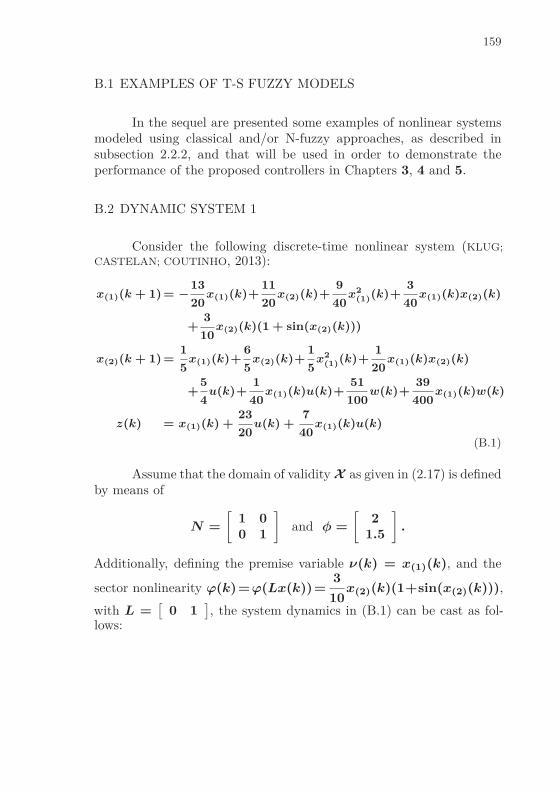
159
B.1 EXAMPLES OF T-S FUZZY MODELS
In the sequel are presented some examples of nonlinear systemsmodeled using classical and/or N-fuzzy approaches, as described insubsection 2.2.2, and that will be used in order to demonstrate theperformance of the proposed controllers in Chapters 3, 4 and 5.
B.2 DYNAMIC SYSTEM 1
Consider the following discrete-time nonlinear system (KLUG;
CASTELAN; COUTINHO, 2013):
x(1)(k + 1) = −13
20x(1)(k)+
11
20x(2)(k)+
9
40x2
(1)(k)+3
40x(1)(k)x(2)(k)
+3
10x(2)(k)(1 + sin(x(2)(k)))
x(2)(k + 1) =1
5x(1)(k)+
6
5x(2)(k)+
1
5x2
(1)(k)+1
20x(1)(k)x(2)(k)
+5
4u(k)+
1
40x(1)(k)u(k)+
51
100w(k)+
39
400x(1)(k)w(k)
z(k) = x(1)(k) +23
20u(k) +
7
40x(1)(k)u(k)
(B.1)
Assume that the domain of validity X as given in (2.17) is definedby means of
N =[
1 00 1
]
and φ =[
21.5
]
.
Additionally, defining the premise variable ν(k) = x(1)(k), and the
sector nonlinearity ϕ(k)=ϕ(Lx(k))=3
10x(2)(k)(1+sin(x(2)(k))),
with L =[
0 1]
, the system dynamics in (B.1) can be cast as fol-lows:

160
x(k + 1) =
−13
20
11
201
5
6
5
+ν(k)
9
40
3
401
5
1
20
x(k) +
[
1
0
]
ϕ(k)
+
[
0
5
4
]
+ν(k)
[
0
1
40
]
u(k)+
[
0
51
100
]
+ν(k)
[
0
39
200
]
w(k)
z(k) = x(1)(k) +
(
23
20+
7
40ν(k)
)
u(k)
(B.2)
where x(k) =[
x(1)(k) x(2)(k)]
′
.Note that the nonlinearity ϕ(k) can be globally encompassed
into a sector bounded nonlinearity, i.e., ϕ(k) ∈ S[0, 0.7], as shown inFigure 42.
x(2)
ϕ = 310
x(2)(1 + sin(x(2))) 0.7x(2)
Figure 42 – Global sector for ϕ = 310
x(2)(1 + sin(x(2)))
Also, it can be observed that ν(k) ∈ [d1, d2], with d1 = −2 andd2 = 2 being the extremum points of ν(k) for the domain X . Thus,the system in (B.2) can be exactly described by the following N-fuzzymodel:

161
x(k + 1) =
2∑
i=1
h(i)(k)Aix(k)+Biu(k)+Bwiw(k)+Giϕ(k)
z(k) =
2∑
i=1
h(i)(k)Czix(k)+Bziu(k)+Bzwiw(k)+Gziϕ(k)
(B.3)
with h(1)(k) =d2 − ν(k)
d2 − d1
, h(2)(k) =ν(k) − d1
d2 − d1
, and the following
system matrices, for i = 1, 2:
Ai =
−13
20+
9
40di
11
20+
3
40di
1
5+
1
5di
6
5+
1
20di
, Bi =
0
5
4+
1
40di
Bwi =
051
100+
39
200di
, Gi = G =
[
1
0
]
Czi =Cz =[
1 0]
, Bzi =23
20+
7
40di, Bzwi =0 and Gzi =0.
B.3 DYNAMIC SYSTEM 2
Consider the control problem of backing-up a truck-trailer asstudied in (FENG; MA, 2001; LO; LIN, 2003; KLUG; CASTELAN; COUTI-
NHO, 2015b). The state space representation of the system is describedby
x(1)(k + 1) = x(1)(k) −vT
Lsin(x(1)(k)) +
vT
lu(k)
x(2)(k + 1) = x(2)(k) +vT
Lsin(x(1)(k)) + 0.2w(k)
x(3)(k + 1) = x(3)(k) + vT cos(x(1)(k)) sin(x(2)(k)
+vT
2Lsin(x(1)(k))) + 0.1w(k)
z(k) = 7x(1)(k) − vT x(2)(k) + 0.03x(3)(k) −vT
lu(k)
(B.4)

162
where x(1)(k) represents the angle between the truck and the trailer,x(2)(k) denotes the angle of the trailer, x(3)(k) is the vertical positionof the rear, and l and L represent the length of the vehicle and ofthe trailer, respectively. T is the sampling time, and v the constantreverse speed. In particular, we consider l = 2.8m, L = 5.5m,v = −1.0m/s and T = 2.0s. Due to physical limitations and/or toguarantee a safe operation of the system, such as preventing the jack-knife effect that occurs when x(1)(k) = ±π/2, the considered domainof validity X in (2.17) is defined as follows (LO; LIN, 2003)
N =[
1 0 00 1 0
]
and φ =[
π
3
170π
180
]′
.
Then, by defining the premise variables
ν(1)(k) =sin(x(1)(k))
x(1)(k), ν(2)(k) =
cos(x(1)(k))
x(1)(k), ν(3)(k) =
sin(ρ(k))
ρ(k),
with ρ = x(2)(k) + vT
2Lsin(x(1)(k)), and observing that ν(1)(k) ∈
[b1, b2], ν(2)(k) ∈ [d1, d2] and ν(3)(k) ∈ [g1, g2] for the considereddomain X , with b1 = 1, b2 = 0.827, d1 = 1, d2 = 0.5, g1 = 1 andg2 = 10−2/π, it is obtained the following classical T-S model of thesystem (B.4) with eight linear local rules
x(k + 1) =8∑
i=1
h(i)(k) (Aix(k) + Biu(k) + Bwiw(k))
z(k) = Czx(k) + Bzu(k) + Bzww(k)(B.5)
where
Ai =Ajkl =
1 −vT
Lbj 0 0
vT
Lbj 1 0
v2T 2
2Lbjdkgl vT dkgl 1
,
Bi = B =
vT
l0
0
, Bwi = Bw =
0
0.2
0.1
,

163
Cz =[
7 −2 0.03]
, Bz = −vT
l, and Bzw = 0,
with i = l + 2(k − 1) + 4(j − 1), for j, k, l = 1, 2. The member-ship functions h(i)(k), i = 1, ..., 8, are the binary product betweenfunctions M i
j , j = 1, 2 and i = 1, 2, 3, defined as:
M11 =
sin(x(1)(k)) − b2x(1)(k)
x(1)(k)(b1 − b2), x(1)(k) 6= 0
1, x(1)(k) = 0
, M12 = 1 − M1
1 ,
M21 =
cos(x(1)(k)) − d2
d1 − d2
, M22 = 1 − M2
1 and
M31 =
sin(ρ) − g2ρ
ρ(g1 − g2), ρ 6= 0
1, ρ = 0, M3
2 = 1 − M31 .
B.4 DYNAMIC SYSTEM 3
Consider the following discrete-time nonlinear system (KLUG;
CASTELAN; COUTINHO, 2015):
x(1)(k + 1) =3
10x(1)(k)−
1
2x(2)(k)−
1
10x2
(1)(k)+1
4x(1)(k)x(2)(k)
+3
10x(2)(k)(1 + sin(x(2)(k)))+
7
10u(k)+
1
20x(1)(k)u(k)
−1
2w(1)(k)−
1
4x(1)(k)w(1)(k)−
11
20w(2)(k)+
7
40x(1)(k)w(2)(k)
x(2)(k + 1) =1
20x(1)(k)−
3
10x(2)(k)+
9
40x2
(1)(k)−1
10x(1)(k)x(2)(k)
−1
20u(k)+
1
40x(1)(k)u(k)+
9
10w(1)(k)+
9
20x(1)(k)w(1)(k)
+1
20w(2)(k)+
19
40x(1)(k)w(2)(k)
(B.6)
Assume that the domain of validity X as given in (2.17) is definedby means of
N =[
1 00 1
]
and φ =[
21.5
]
.

164
i) Classical T-S Modeling: Defining the premise variables ν(1)(k) =x(1)(k) and ν(2)(k) = sin x(1)(k), the system dynamics in (B.6) canbe cast as follows:
x(k + 1) =
−1
2−
11
209
10
1
40
+ ν(1)(k)
−1
4
7
409
20
19
40
w(k)
+
3
10−
1
51
20−
3
10
+ν(1)(k)
−1
10
1
49
40−
1
10
+ν(2)(k)
03
10
0 0
x(k)
+
7
10
−1
20
+ν(1)(k)
1
201
40
u(k).
(B.7)
where x(k)=[
x(1)(k) x(2)(k)]
′
and w(k)=[
w(1)(k) w(2)(k)]
′
.In the domain X , the maximum and minimum values of the
premise variables are such that ν(1)(k) ∈ [d1, d2], with d1 = −2 andd2 = 2, and ν(2)(k) ∈ [e1, e2], with e1 = −0.998 and e2 = 0.998.Thus, the system in (B.6) can be exactly described by the followingclassical T-S fuzzy model:
x(k + 1) =4∑
i=1
hk(i) (Aix(k) + Biu(k) + Bwiw(k)) (B.8)
where, for j, l = 1, 2 and i = l + 2(j − 1):
Ai =
3
10−
1
10dj −
1
5+
1
4dj +
3
10el
1
20+
9
40dj −
3
10−
1
10dj
,
Bi =
7
10+
1
20dj
−1
20+
1
40dj
, Bwi =
−1
2−
1
4dj −
11
20+
7
40dj
9
10+
9
20dj
1
40+
19
40dj
.
The membership functions h(i)(k), i = 1, ..., 4, are the binary product

165
between functions M ij , j = 1, 2 and i = 1, 2, defined as:
M11 =
d2 − ν(1)(k)
d2 − d1
, M12 =
ν(1)(k) − d1
d2 − d1
,
M21 =
e2 − ν(2)(k)
e2 − e1
, M22 =
ν(2)(k) − e1
e2 − e1
.
ii) N-Fuzzy Modeling: Considering the sector nonlinearity ϕ(k) =
ϕ(Lx(k)) =3
10x(2)(k)(1+sin(x(2)(k))), and by defining the pre-
misse variable ν(k) = x(1)(k), the system dynamics in (B.6) can becast as follows:
x(k + 1) =
3
10−
1
21
20−
3
10
+ν(k)
−1
10
1
49
40−
1
10
x(k) +
[
1
0
]
ϕ(k)
+
−1
2−
11
209
10
1
40
+ ν(1)(k)
−1
4
7
409
20
19
40
w(k)
+
7
10
−1
20
+ν(k)
1
201
40
u(k)
(B.9)
where x(k)=[
x(1)(k) x(2)(k)]
′
and w(k)=[
w(1)(k) w(2)(k)]
′
.Notice that the nonlinearity ϕ(k) is the same as that presented
in the dynamic system 1, therefore it can be globally encompassedinto a sector bounded nonlinearity, i.e., ϕk ∈ S[0, 0.7], as well asν(k) ∈ [d1, d2], with d1 = −2 and d2 = 2 being the extremumpoints for ν(k) in the domain X . Thus, the system in (B.9) can beexactly described by the following N-fuzzy model:
x(k + 1) =2∑
i=1
hk(i) (Aix(k) + Biu(k) + Bwiw(k) + Giϕk)
(B.10)where, for i = 1, 2:
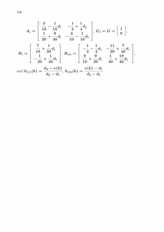
166
Ai =
3
10−
1
10di −
1
2+
1
4dj
1
20+
9
40di −
3
10−
1
10di
, Gi = G =[
10
]
,
Bi =
7
10+
1
20di
−1
20+
1
40di
, Bwi =
−1
2−
1
4di −
11
20+
7
40di
9
10+
9
20di
1
40+
19
40di
,
and h(1)(k) =d2 − ν(k)
d2 − d1
, h(2)(k) =ν(k) − d1
d2 − d1
.

APPENDIX C -- Mesh Transformation

169
C.1 TRANSFORMATION ϕ ∈ [Ω1, Ω2] IN ϕ ∈ [0, Ω]
This appendix demonstrates a transformation process with sec-tor nonlinearities which is required to compatibilize the representationgiven in (2.6) with the condition (2.3).
Let ϕ(k) = ϕ(Lx(k)) a vector of nonlinearities belonging tothe bounded sector condition ϕ(.) ∈ [Ω1, Ω2], i.e. for the matrices Ω1
and Ω2 the following condition is satisfied
[ϕ(k) − Ω1Lx(k)]′
∆−1[ϕ(k) − Ω2Lx(k)] ≤ 0, ϕ(0) = 0. (C.1)
Defining ϕ(k) = ϕ(k) − Ω1Lx(k) ⇒ ϕ(k) = ϕ(k) + Ω1Lx(k) andreplacing in (C.1), leads to
ϕ′
(k)∆−1[ϕ(k) − (Ω2 − Ω1)Lx(k)] ≤ 0.
If Ω = Ω2 − Ω1, then the mesh transformation ϕ ∈ [Ω1, Ω2] inϕ ∈ [0, Ω] is computed by
ϕ′
(k)∆−1[ϕ(k) − ΩLx(k)] ≤ 0, ϕ(0) = 0,Ω = Ω2 − Ω1 e ϕ(k) = ϕ(k) − Ω1Lx(k)
(C.2)
Example 1 - Sector nonlinearity ϕ = sin(x), L = 1: It ispossible to verify the for the region |x| ≤ d, with d = 2π/3, thenonlinearity is encompassed into the bounded sector
ϕ(.) ∈ [Ω1, Ω2], Ω1 =sin(2π/3)
2π/3and Ω2 = 1.
Applying the mesh transformation elucidated in (C.2), it is obtained
ϕ = sin(x) −sin(2π/3)
2π/3x, belonging to the bounded sector
ϕ(.) ∈ [0, Ω], Ω = Ω2 − Ω1, for |x| ≤ d.
A graphic description of the transformation process can be seenin Figure 43.
Example 2: - Effect upon the system matrices: Let the subsys-tems described by:
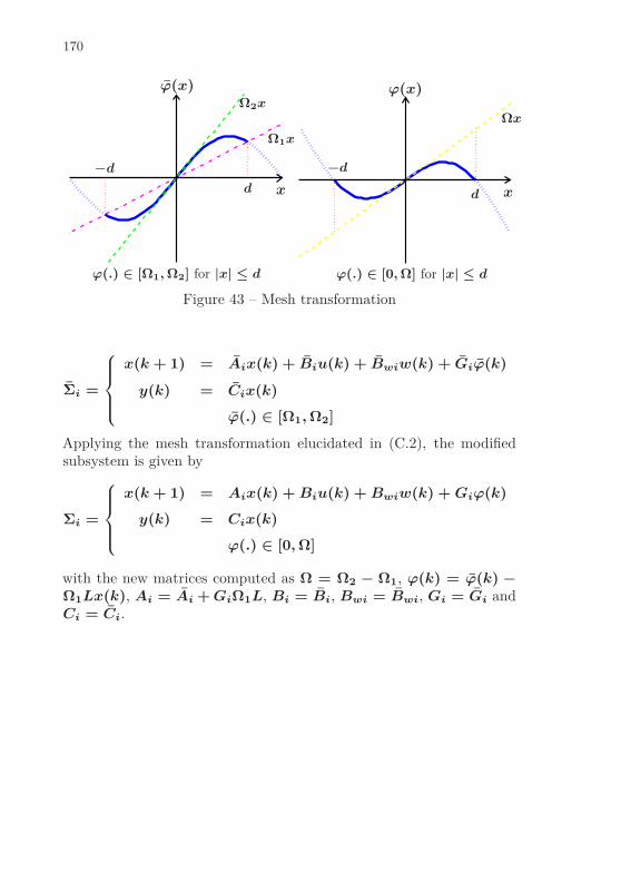
170
x
ϕ(x)
Ω1x
Ω2x
d
−d
ϕ(.) ∈ [Ω1, Ω2] for |x| ≤ d
x
ϕ(x)
Ωx
d
−d
ϕ(.) ∈ [0, Ω] for |x| ≤ d
Figure 43 – Mesh transformation
Σi =
x(k + 1) = Aix(k) + Biu(k) + Bwiw(k) + Giϕ(k)
y(k) = Cix(k)
ϕ(.) ∈ [Ω1, Ω2]
Applying the mesh transformation elucidated in (C.2), the modifiedsubsystem is given by
Σi =
x(k + 1) = Aix(k) + Biu(k) + Bwiw(k) + Giϕ(k)
y(k) = Cix(k)
ϕ(.) ∈ [0, Ω]
with the new matrices computed as Ω = Ω2 − Ω1, ϕ(k) = ϕ(k) −Ω1Lx(k), Ai = Ai + GiΩ1L, Bi = Bi, Bwi = Bwi, Gi = Gi andCi = Ci.

APPENDIX D -- Conditions of Literature and NumericalComplexity Analysis

173
D.1 CONDITIONS OF LITERATURE
In the following, stabilization conditions for nonlinear systemsrepresented by T-S fuzzy models deriving from literature works arepresented. The structure of this appendix is as follows: conditions inSections D.2.1 and D.2.2 deals with state feedback problem and wereused to perform a Numerical Complexity Analysis in Section D.2.3, alsogenerating the comparative Tables 6 and 7. Section D.3 deals with thedynamic output feedback problem and their conditions were used inthe Illustrative Example 2.3.
D.2 NUMERICAL COMPLEXITY
It is noteworthy that the numerical complexity for the solutionof LMI-based optimization problems is related to the number of scalardecision variables, K , and the number of rows, L, of the consideredLMIs. The number of floating point operations (FLOP) or the time re-quired to solve a problem, using interior point methods, is proportionalto K 3L (GAHINET et al., 1995; LEITE et al., 2004).
For comparison purposes, the following conditions, associatedwith literature control laws, are considered:
D.2.1 Adapted conditions of Klug & Castelan (2011)
The results presented below are stabilization conditions based inthe work Klug & Castelan (2011). For this case are considered nonlinearsystems that can be represented by N-fuzzy models, as described in(2.5). The proposed control law is based on the feedback of states andsector nonlinearities, given by
u(k) = K(h(k))x(k) + Γ(h(k))ϕ(k). (D.1)
It is interesting to note that these conditions effectively do notguarantee the closed-loop stability when applied to the original nonli-near system, since the additional condition that deal with the regionalvalidity issue is not taken into consideration. Such factor is required toexist a fair comparison regarding the techniques from literature.
Proposition 2 in Klug & Castelan (2011) - Adapted: Given areal scalar λ ∈ (0, 1], suppose that there exists symmetric positive defi-
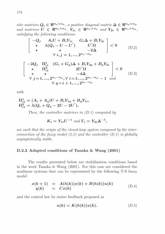
174
nite matrices Qi ∈ ℜnx×nx , a positive diagonal matrix ∆ ∈ ℜnϕ×nϕ
and matrices U ∈ ℜnx×nx , Y1i ∈ ℜnu×nx and Y2i ∈ ℜnu×nϕ ,satisfying the following conditions:
−Qj AiU + BiY1i Gi∆ + BiY2i
⋆ λ(Qi − U − U′
) U′
Ω⋆ ⋆ −2∆
< 0
∀ i, j = 1, ..., 2ns−nϕ
(D.2)
−2Qj Π1i1 (Gi + Gq)∆ + BiY2q + BqY2i
⋆ Π2i1 2U
′
Ω⋆ ⋆ −4∆
< 0
∀ j =1, ..., 2ns−nϕ , ∀ i=1, ..., 2ns−nϕ − 1 and∀ q = i + 1, ..., 2ns−nϕ
(D.3)
with
Π1i1 = (Ai + Aq)U + BiY1q + BqY1i,
Π2i1 = λ(Qi + Qq − 2U − 2U
′
).
Then, the controller matrices in (D.1) computed by
Ki = Y1iU−1 and Γi = Y2i∆−1,
are such that the origin of the closed-loop system composed by the inter-connection of the fuzzy model (2.5) and the controller (D.1) is globallyasymptotically stable.
D.2.2 Adapted conditions of Tanaka & Wang (2001)
The results presented below are stabilization conditions basedin the work Tanaka & Wang (2001). For this case are considered thenonlinear systems that can be represented by the following T-S fuzzymodel
x(k + 1) = A(h(k))x(k) + B(h(k))u(k)y(k) = Cx(k)
(D.4)
and the control law by states feedback proposed as
u(k) = K(h(k))x(k). (D.5)
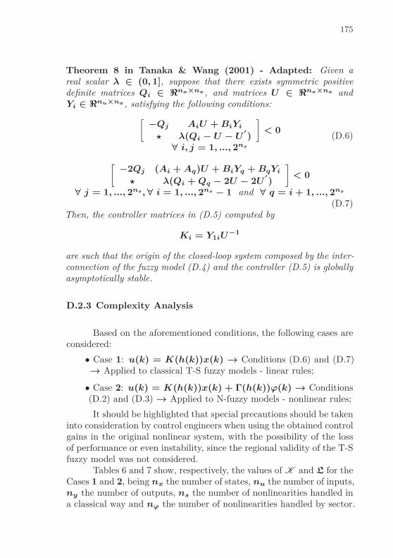
175
Theorem 8 in Tanaka & Wang (2001) - Adapted: Given areal scalar λ ∈ (0, 1], suppose that there exists symmetric positivedefinite matrices Qi ∈ ℜnx×nx , and matrices U ∈ ℜnx×nx andYi ∈ ℜnu×nx , satisfying the following conditions:
[
−Qj AiU + BiYi
⋆ λ(Qi − U − U′
)
]
< 0
∀ i, j = 1, ..., 2ns
(D.6)
[
−2Qj (Ai + Aq)U + BiYq + BqYi
⋆ λ(Qi + Qq − 2U − 2U′
)
]
< 0
∀ j = 1, ..., 2ns , ∀ i = 1, ..., 2ns − 1 and ∀ q = i + 1, ..., 2ns
(D.7)Then, the controller matrices in (D.5) computed by
Ki = Y1iU−1
are such that the origin of the closed-loop system composed by the inter-connection of the fuzzy model (D.4) and the controller (D.5) is globallyasymptotically stable.
D.2.3 Complexity Analysis
Based on the aforementioned conditions, the following cases areconsidered:
• Case 1: u(k) = K(h(k))x(k) → Conditions (D.6) and (D.7)→ Applied to classical T-S fuzzy models - linear rules;
• Case 2: u(k) = K(h(k))x(k) + Γ(h(k))ϕ(k) → Conditions(D.2) and (D.3) → Applied to N-fuzzy models - nonlinear rules;
It should be highlighted that special precautions should be takeninto consideration by control engineers when using the obtained controlgains in the original nonlinear system, with the possibility of the lossof performance or even instability, since the regional validity of the T-Sfuzzy model was not considered.
Tables 6 and 7 show, respectively, the values of K and L for theCases 1 and 2, being nx the number of states, nu the number of inputs,ny the number of outputs, ns the number of nonlinearities handled ina classical way and nϕ the number of nonlinearities handled by sector.
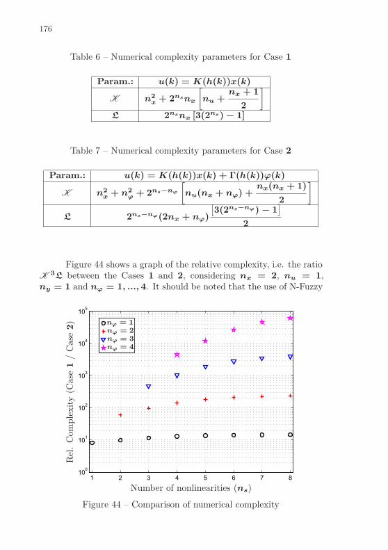
176
Table 6 – Numerical complexity parameters for Case 1
Param.: u(k) = K(h(k))x(k)
K n2x + 2nsnx
[
nu +nx + 1
2
]
L 2nsnx [3(2ns) − 1]
Table 7 – Numerical complexity parameters for Case 2
Param.: u(k) = K(h(k))x(k) + Γ(h(k))ϕ(k)
K n2x + n2
ϕ + 2ns−nϕ
[
nu(nx + nϕ) +nx(nx + 1)
2
]
L 2ns−nϕ(2nx + nϕ)
[
3(2ns−nϕ) − 1]
2
Figure 44 shows a graph of the relative complexity, i.e. the ratioK 3L between the Cases 1 and 2, considering nx = 2, nu = 1,ny = 1 and nϕ = 1, ..., 4. It should be noted that the use of N-Fuzzy
1 2 3 4 5 6 7 810
0
101
102
103
104
105
Number of nonlinearities (ns)
Rel
.C
ompl
exit
y(C
ase
1/
Cas
e2) nϕ = 1
nϕ = 2
nϕ = 3
nϕ = 4
Figure 44 – Comparison of numerical complexity

177
models (Case 2) provides a meaningful numerical complexity reductioncompared to classical T-S fuzzy models (Case 1), which becomes morepronounced with an increase in nϕ. This characteristic is explained bythe rule reduction provided by the nonlinear approach, dominant overthe generation of new decision variables, such as ∆ and Y2i.
D.3 ADAPTED CONDITIONS OF FENG (2010)
The results presented below are stabilization conditions basedin the work Feng (2010). For comparison purposes, the conditionswere adapted to handle with the stabilization problem, considering thefollowing fuzzy representation of the nonlinear system (2.1)
x(k + 1) = A(h(k))x(k) + B(h(k))u(k)y(k) = C(h(k))x(k)
(D.8)
in which the definition of variables and functions are identical as thoseestablished in equation (3.1). The dynamic output feedback controlleris defined by
xc(k + 1) = A(h(k))xc(k) + B(h(k))y(k)u(k) = C(h(k))xc(k)
(D.9)
where it should be emphasized that the matrix structure of Ac(h(k)),Bc(h(k)) and Cc(h(k)) are not the same as in (3.7). The candidatefuzzy Lyapunov function is
V (ξ(k)) = ξ′
(k)
(
nr∑
i=1
h(i)(k)X−1i
)
ξ(k). (D.10)
Theorem 8.10 in Feng (2010) - Adapted: The closed-loop sys-tem, formed by the T-S fuzzy model (D.8) and the controller (D.9), isglobally exponentially stable if exists the positive definite matrices
Xi =[
Xi1 ⋆
Xi2 Xi3
]
, ∀i = 1, ..., nr,

178
and matrices G1, U1, M , Ai, Bi, Ci, ∀i = 1, ..., nr, such that thefollowing LMIs are verified:
Xi1 − G1 − G′
1 ⋆ ⋆ ⋆
Xi2 − M − I Xi3 − U1 − U′
1 ⋆ ⋆
AiG1 + B1i~Cj Ai −Xl1 ⋆
~Ai U1Ai + ~BrCi −Xl2 −Xl3
≤ 0
∀ i, j, r, l = 1, ..., nr
Furthermore, the controller gains can be computed by
A(h(k)) =(
~A(h(k)) − U1A(h(k))G1 − ~B(h(k))C(h(k))G1
−U1B1(h(k)) ~C(h(k)))
(M − U1G1)−1,
B(h(k)) = ~B(h(k)),
C(h(k)) = ~C(h(k)) (M − U1G1)−1,
with[
~A (h(k)) ~B (h(k)) ~C (h(k)) A (h(k)) B (h(k)) C (h(k))]
=nr∑
i=1
h(i)(k)[
~Ai~Bi
~Ci Ai Bi Ci
]
.
Proof The procedures used for determining the conditions of the abovetheorem can be found in Chapter 8 of the work Feng (2010).

APPENDIX E -- Projections


181
E.1 PROJECTION OF AN ELLIPSOID
Consider E(P ) a ellipsoid such that ξ′
P ξ ≤ 1, with ξ =[
xxc
]
. It is desired to obtain the projection of this ellipsoid over,
for example, the subspace of x. Thus, for a given E(P ), it has thefollowing decomposition
P =[
P11 P12
P′
12 P22
]
> 0
and the definition
ξ =[
xxc
]
=[
I 0−P −1
22 P′
12 I
] [
xxc
]
.
Notice that P −122 exists, because P > 0. Hence, ξ
′
P ξ ≤ 1 can berewritten as
[
x′
x′
c
]
[
I −P12P −122
0 I
][
P11 P12
P′
12 P22
][
I 0−P −1
22 P′
12 I
][
xxc
]
≤ 1 ⇒
[
x′
x′
c
]
[
P11 − P12P −122 P
′
12 00 P22
] [
xxc
]
≤ 1. (E.1)
Since x and xc are decoupled in equation (E.1), the associated projec-tion can be defined by
Proj [E(P )]over x =
x : x′
(P11 − P12P −122 P
′
12)x ≤ 1
. (E.2)
In this way, the Schur complement of P in relation to P22 pro-vides the orthogonal projection of E(P ) over the portion of space rela-tive to x.
Example - Projection of an ellipse: Let the ellipse given by:
[x y] P [x y]′
≤ 1, P =[
0.3 −0.4−0.4 1
]
, (E.3)
to which it is desired to obtain the orthogonal projections over the axesx and y. Using the definition in (E.2), the projections are equivalent

182
to:
Proj [Ellipse]over x =
x : x′
(P11 − P12P −122 P
′
12)x ≤ 1
⇒ |x| ≤ 2.6726
Proj [Ellipse]over y =
y : y′
(P22 − P′
12P −111 P12)y ≤ 1
⇒ |y| ≤ 1.4639(E.4)
The graphics of the ellipse (represented by a continuous line) andits projections obtained by (E.4) (where the projections over x and yare represented by a dashed and dashed-dotted lines, respectively) areshown in Figure 45.
−3 −2 −1 0 1 2 3
−1.5
−1
−0.5
0
0.5
1
1.5
x
y
Figure 45 – Projection of an ellipse
Example - Projection of an Ellipsoid: Let the generic ellipsoidξ
′
P ξ ≤ 1, with ξ ∈ ℜ3. The Figure 46 represents the ellipsoid trans-lated from the state space origin (for the sake of better visualization),as well as its projection (green ellipse) over a plane formed by the greenand red axes, and the respective intersection over the same plane (redellipse).

183
Figure 46 – Projection of an ellipsoid