Introduction to run Siesta

Javier Junquera

UniversitUniversitéé de Li de Lièègege

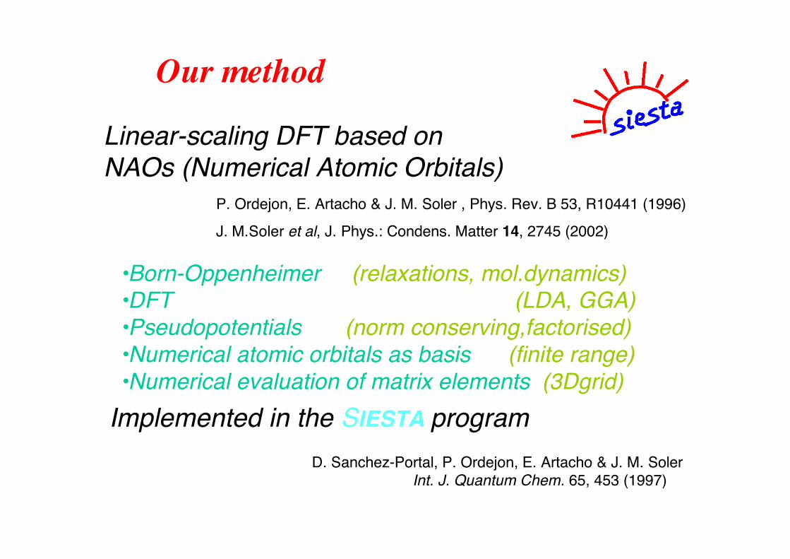
Our method

Linear-scaling DFT based onNAOs (Numerical Atomic Orbitals)

P. Ordejon, E. Artacho & J. M. Soler , Phys. Rev. B 53, R10441 (1996)J. M.Soler et al, J. Phys.: Condens. Matter 14, 2745 (2002)

•Born-Oppenheimer (relaxations, mol.dynamics)•DFT (LDA, GGA)•Pseudopotentials (norm conserving,factorised)•Numerical atomic orbitals as basis (finite range)•Numerical evaluation of matrix elements (3Dgrid)

Implemented in the SIESTA programD. Sanchez-Portal, P. Ordejon, E. Artacho & J. M. Soler Int. J. Quantum Chem. 65, 453 (1997)

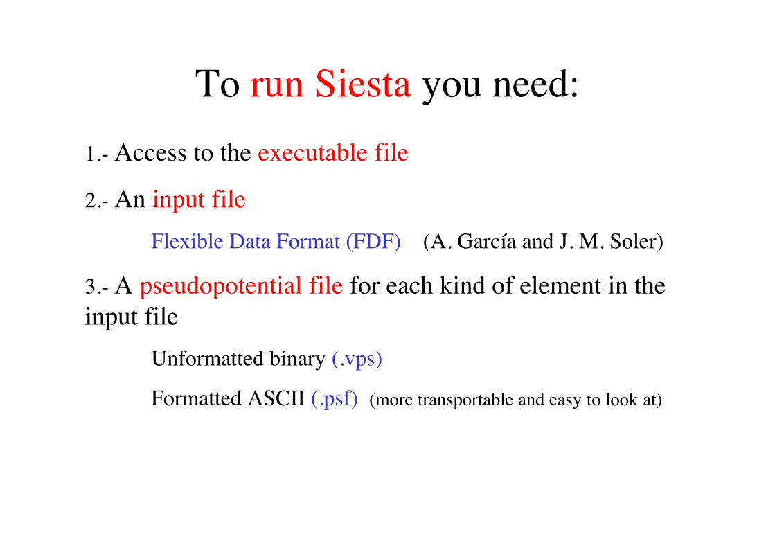
To run Siesta you need:1.- Access to the executable file

2.- An input fileFlexible Data Format (FDF) (A. García and J. M. Soler)

3.- A pseudopotential file for each kind of element in theinput file

Unformatted binary (.vps)

Formatted ASCII (.psf) (more transportable and easy to look at)

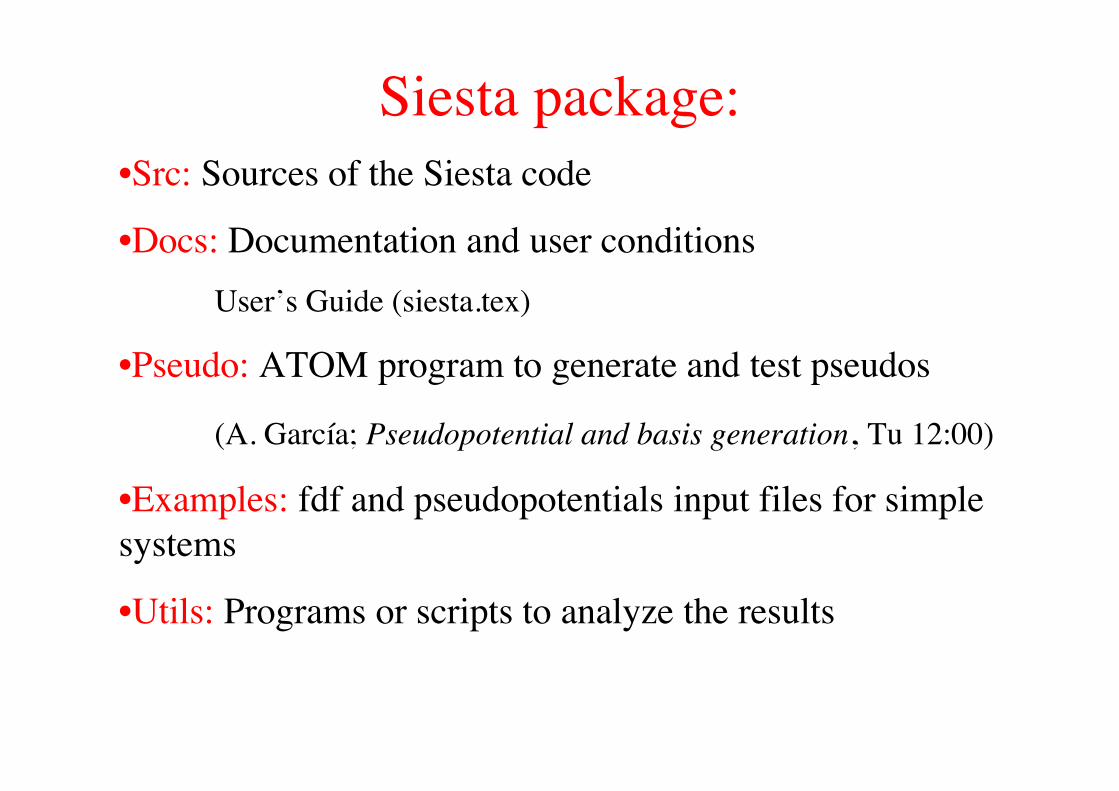
Siesta package:•Src: Sources of the Siesta code

•Docs: Documentation and user conditionsUser’s Guide (siesta.tex)

•Pseudo: ATOM program to generate and test pseudos

(A. García; Pseudopotential and basis generation, Tu 12:00)

•Examples: fdf and pseudopotentials input files for simplesystems

•Utils: Programs or scripts to analyze the results

The input file

Main input file:

•Physical data of the system

•Variables to control the approximations

•Flexible Data Format (FDF)

developped by A. García and J. M. Soler

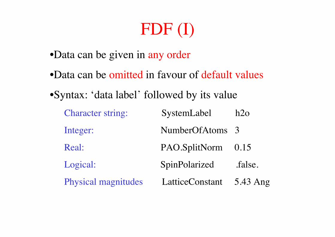
FDF (I)•Data can be given in any order

•Data can be omitted in favour of default values

•Syntax: ‘data label’ followed by its valueCharacter string: SystemLabel h2o

Integer: NumberOfAtoms 3

Real: PAO.SplitNorm 0.15

Logical: SpinPolarized .false.

Physical magnitudes LatticeConstant 5.43 Ang

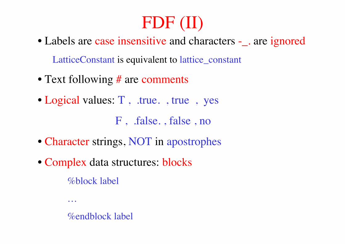
FDF (II)• Labels are case insensitive and characters -_. are ignored

LatticeConstant is equivalent to lattice_constant

• Text following # are comments

• Logical values: T , .true. , true , yes

F , .false. , false , no

• Character strings, NOT in apostrophes

• Complex data structures: blocks%block label

…

%endblock label

FDF (III)• Physical magnitudes: followed by its units.

Many physical units are recognized for each magnitude

(Length: m, cm, nm, Ang, bohr)

Automatic conversion to the ones internally required.

• You may ‘include’ other FDF files or redirect the searchto another file

Basic input variables

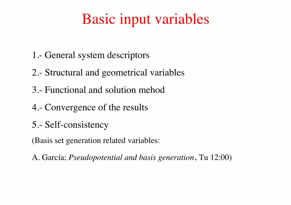
1.- General system descriptors

2.- Structural and geometrical variables

3.- Functional and solution mehod

4.- Convergence of the results

5.- Self-consistency(Basis set generation related variables:

A. García; Pseudopotential and basis generation, Tu 12:00)

General system descriptor

SystemName: descriptive name of the systemSystemName Si bulk, diamond structure

SystemLabel: nickname of the system to name output filesSystemLabel Si

(After a succesful run, you should have files like

Si.DM : Density matrix

Si.XV: Final positions and velocities

...)

Structural and geometrical variablesNumberOfAtoms: number of atoms in the simulation

NumberOfAtoms 2

NumberOfSpecies: number of different atomic speciesNumberOfSpecies 1

ChemicalSpeciesLabel: specify the different chemicalspecies.

%block ChemicalSpeciesLabel

1 14 Si

%endblock ChemicalSpeciesLabel

ALL THESE VARIABLES ARE MANDATORY

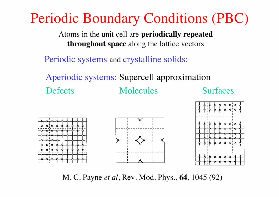
Periodic Boundary Conditions (PBC)

M. C. Payne et al, Rev. Mod. Phys., 64, 1045 (92)

Defects Molecules SurfacesAperiodic systems: Supercell approximation

Atoms in the unit cell are periodically repeatedthroughout space along the lattice vectors

Periodic systems and crystalline solids: ÷

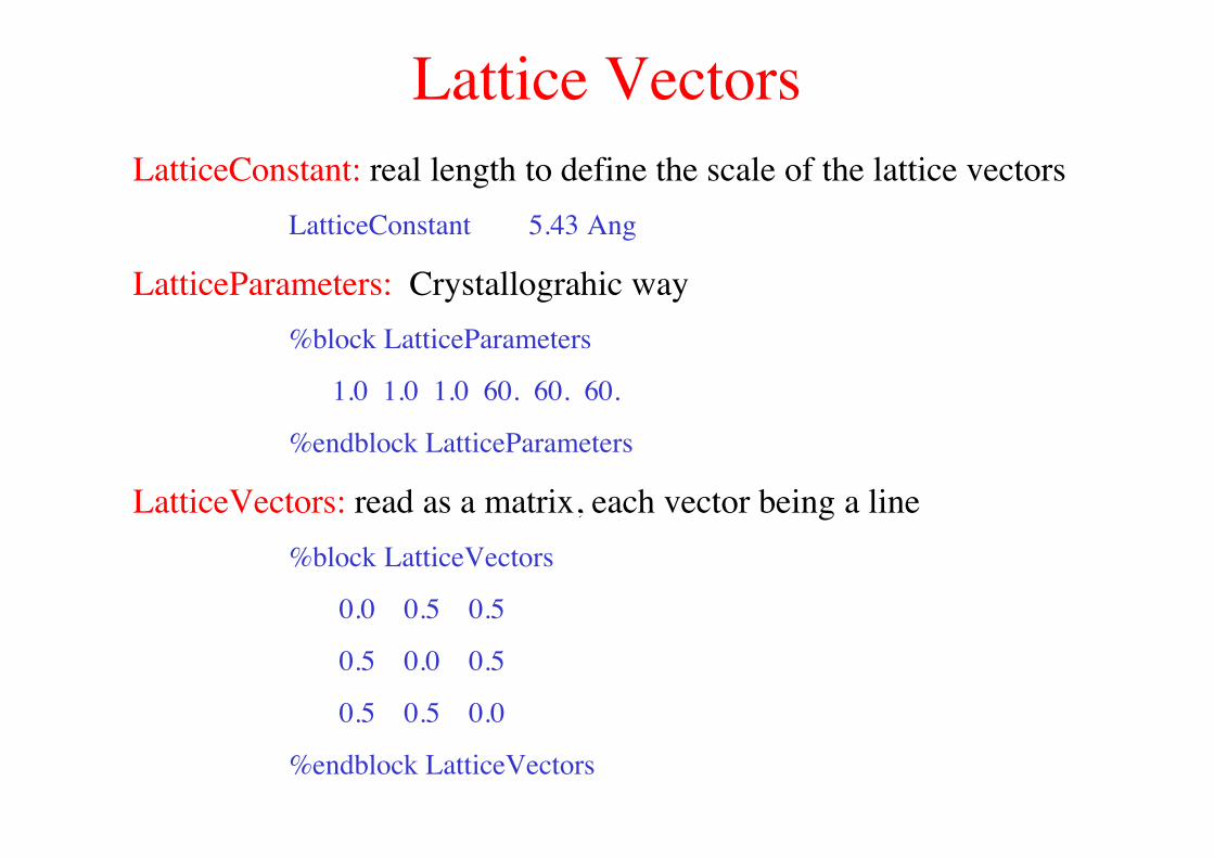
Lattice VectorsLatticeConstant: real length to define the scale of the lattice vectors

LatticeConstant 5.43 Ang

LatticeParameters: Crystallograhic way%block LatticeParameters

1.0 1.0 1.0 60. 60. 60.

%endblock LatticeParameters

LatticeVectors: read as a matrix, each vector being a line%block LatticeVectors

0.0 0.5 0.5

0.5 0.0 0.5

0.5 0.5 0.0

%endblock LatticeVectors

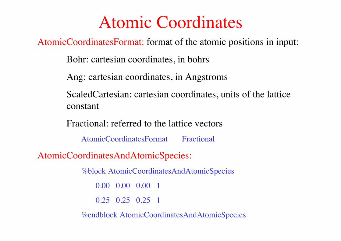
Atomic CoordinatesAtomicCoordinatesFormat: format of the atomic positions in input:

Bohr: cartesian coordinates, in bohrs

Ang: cartesian coordinates, in Angstroms

ScaledCartesian: cartesian coordinates, units of the latticeconstant

Fractional: referred to the lattice vectorsAtomicCoordinatesFormat Fractional

AtomicCoordinatesAndAtomicSpecies:%block AtomicCoordinatesAndAtomicSpecies

0.00 0.00 0.00 1

0.25 0.25 0.25 1

%endblock AtomicCoordinatesAndAtomicSpecies

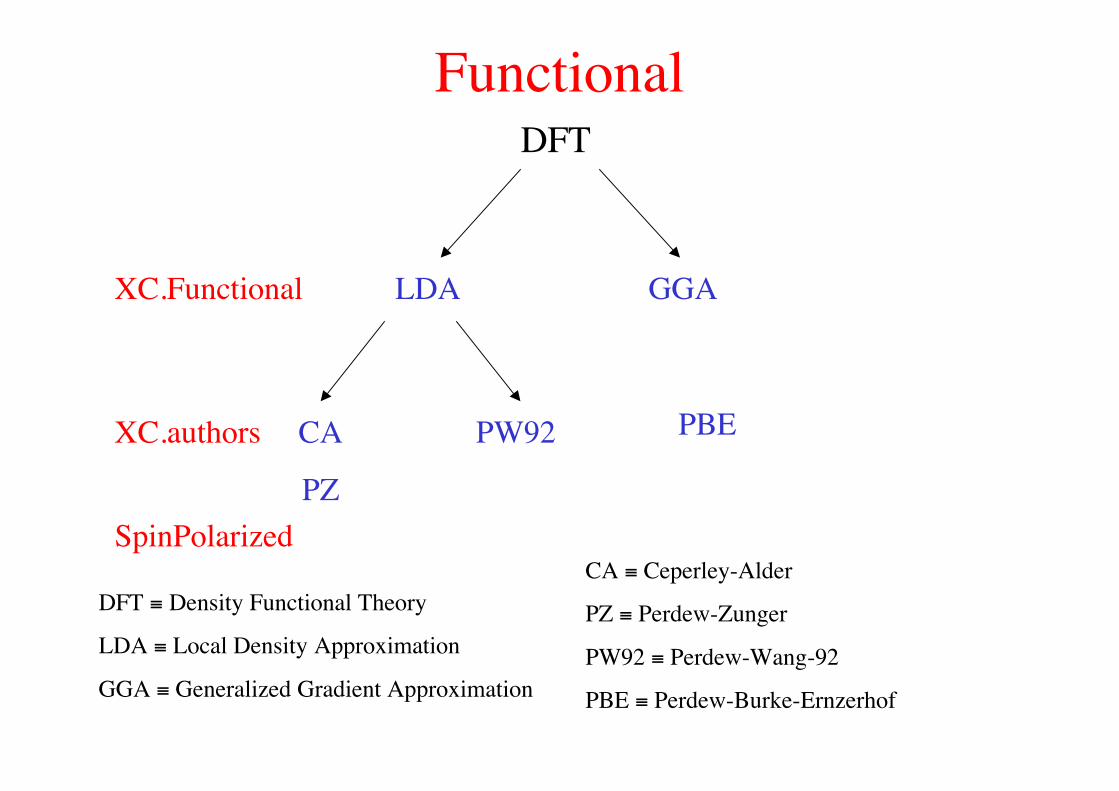
FunctionalDFT

XC.Functional LDA GGA

XC.authors PW92CA

PZ

PBE

DFT ≡ Density Functional Theory

LDA ≡ Local Density Approximation

GGA ≡ Generalized Gradient Approximation

CA ≡ Ceperley-Alder

PZ ≡ Perdew-Zunger

PW92 ≡ Perdew-Wang-92

PBE ≡ Perdew-Burke-Ernzerhof

SpinPolarized

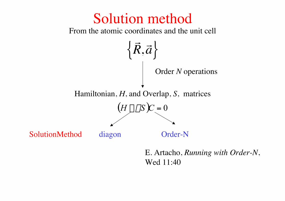
Solution method

r R , r a { }

Hamiltonian, H, and Overlap, S, matrices

Order N operations

( ) 0=- CSH e

SolutionMethod diagon Order-N

From the atomic coordinates and the unit cell

E. Artacho, Running with Order-N,Wed 11:40

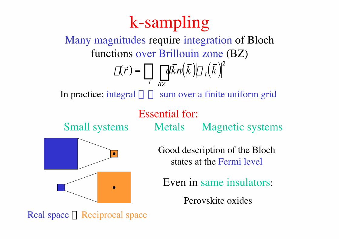
k-samplingMany magnitudes require integration of Bloch

functions over Brillouin zone (BZ)

r

r r ( ) = dr k n

r k ( )

BZÚ

i y i

r k ( )2

In practice: integral æÆ sum over a finite uniform grid

Essential for:Small systems

Real space ´Reciprocal space

Metals Magnetic systems

Good description of the Blochstates at the Fermi level

Even in same insulators:

Perovskite oxides

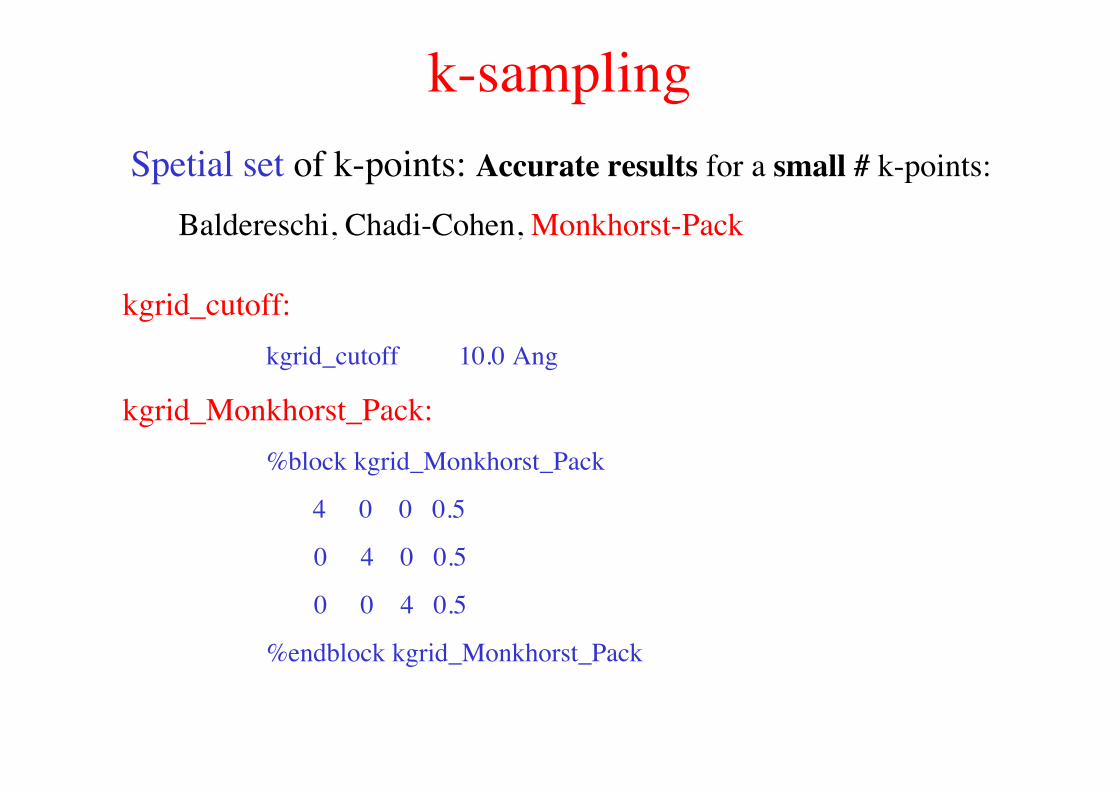
k-sampling

kgrid_cutoff:kgrid_cutoff 10.0 Ang

kgrid_Monkhorst_Pack:%block kgrid_Monkhorst_Pack

4 0 0 0.5

0 4 0 0.5

0 0 4 0.5

%endblock kgrid_Monkhorst_Pack

Spetial set of k-points: Accurate results for a small # k-points:

Baldereschi, Chadi-Cohen, Monkhorst-Pack

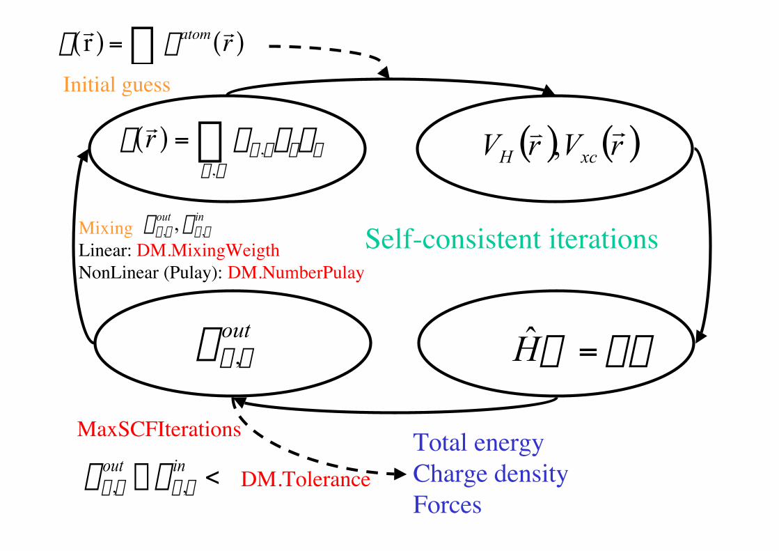
Self-consistent iterations

r

r r ( ) = rm,nfmfnm,n ( ) ( )rVrV xcH

rv,

yey =H

MaxSCFIterations

rr r ( ) = ratom r r ( )Â

Initial guess

outnmr ,

Total energyCharge densityForces

<- inoutnmnm rr ,, DM.Tolerance

Mixing Linear: DM.MixingWeigthNonLinear (Pulay): DM.NumberPulay

inoutnmnm rr ,, ,

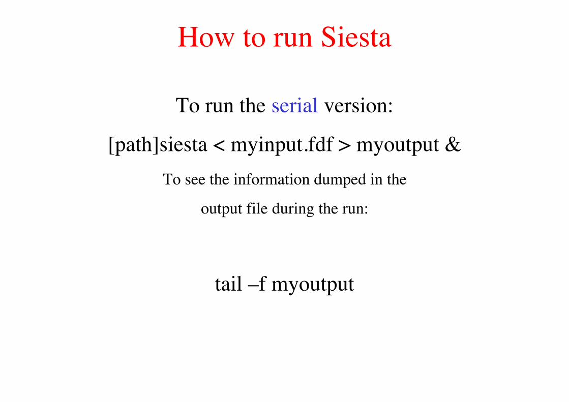
How to run Siesta

To run the serial version:

[path]siesta < myinput.fdf > myoutput &To see the information dumped in the

output file during the run:

tail –f myoutput

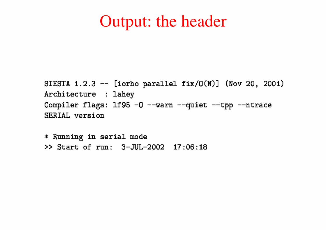
Output: the header

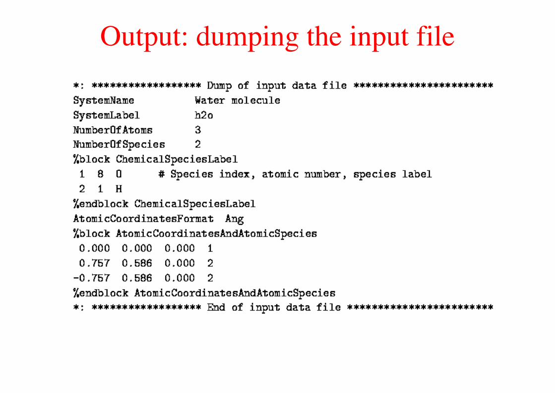
Output: dumping the input file

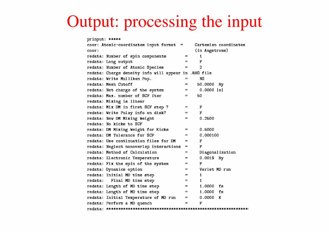
Output: processing the input

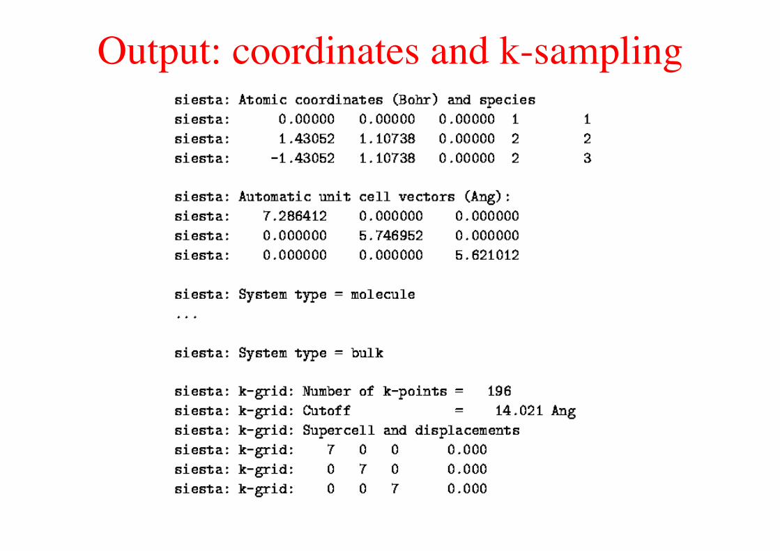
Output: coordinates and k-sampling

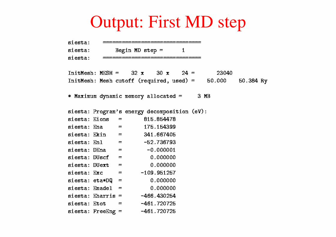
Output: First MD step

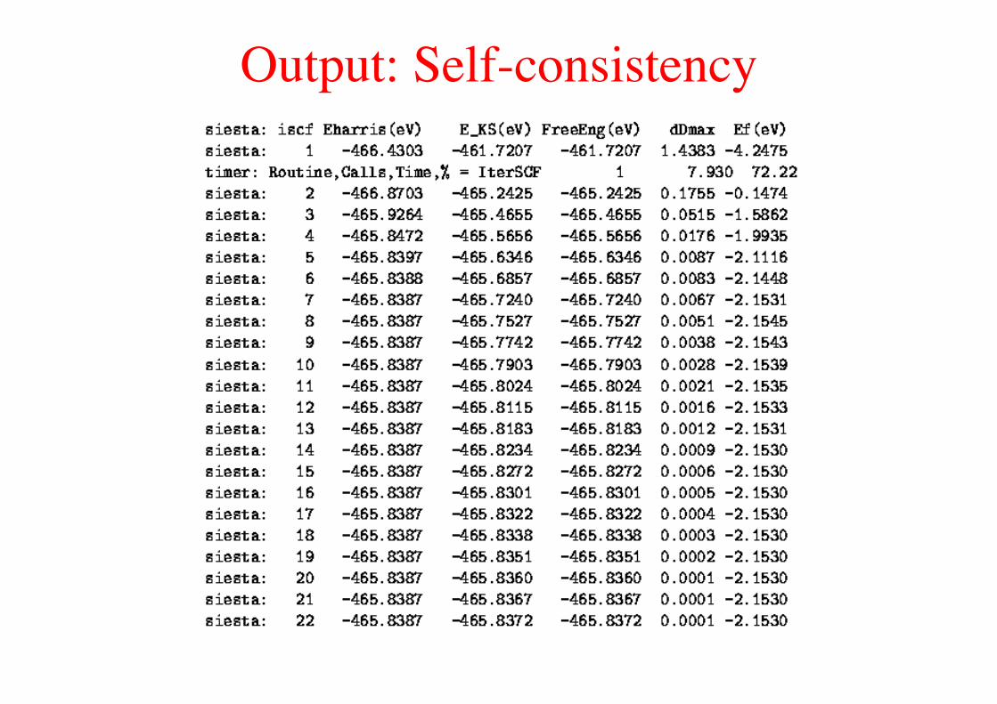
Output: Self-consistency

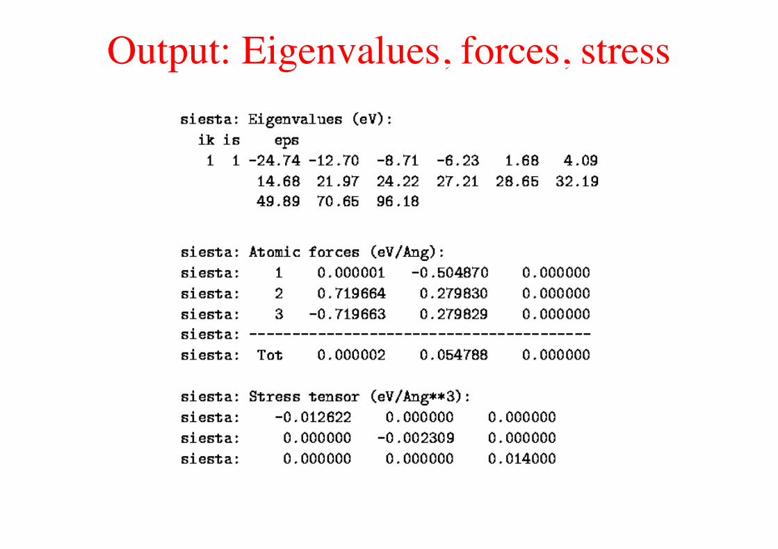
Output: Eigenvalues, forces, stress

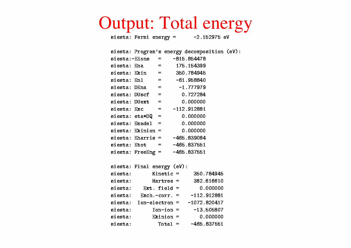
Output: Total energy

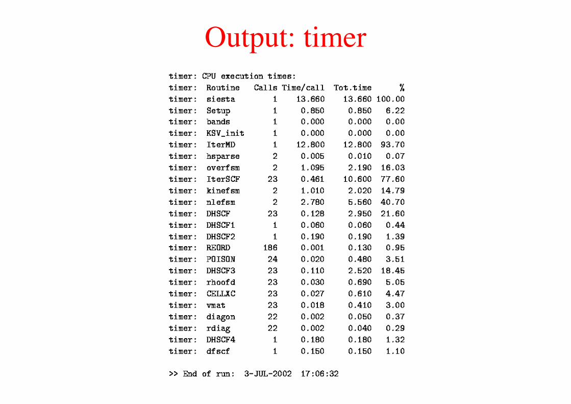
Output: timer

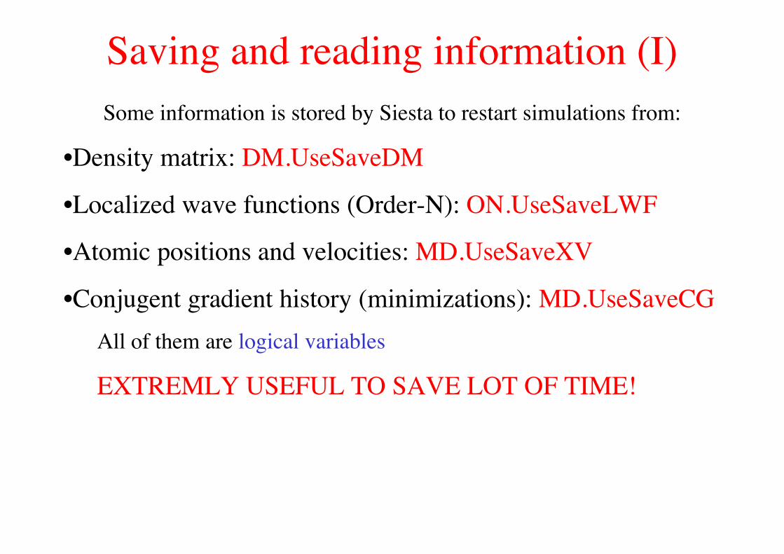
Saving and reading information (I)Some information is stored by Siesta to restart simulations from:

•Density matrix: DM.UseSaveDM

•Localized wave functions (Order-N): ON.UseSaveLWF

•Atomic positions and velocities: MD.UseSaveXV

•Conjugent gradient history (minimizations): MD.UseSaveCGAll of them are logical variables

EXTREMLY USEFUL TO SAVE LOT OF TIME!

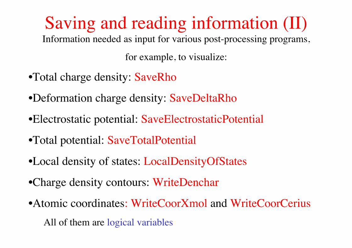
Saving and reading information (II)Information needed as input for various post-processing programs,

for example, to visualize:

•Total charge density: SaveRho

•Deformation charge density: SaveDeltaRho

•Electrostatic potential: SaveElectrostaticPotential

•Total potential: SaveTotalPotential

•Local density of states: LocalDensityOfStates

•Charge density contours: WriteDenchar

•Atomic coordinates: WriteCoorXmol and WriteCoorCeriusAll of them are logical variables

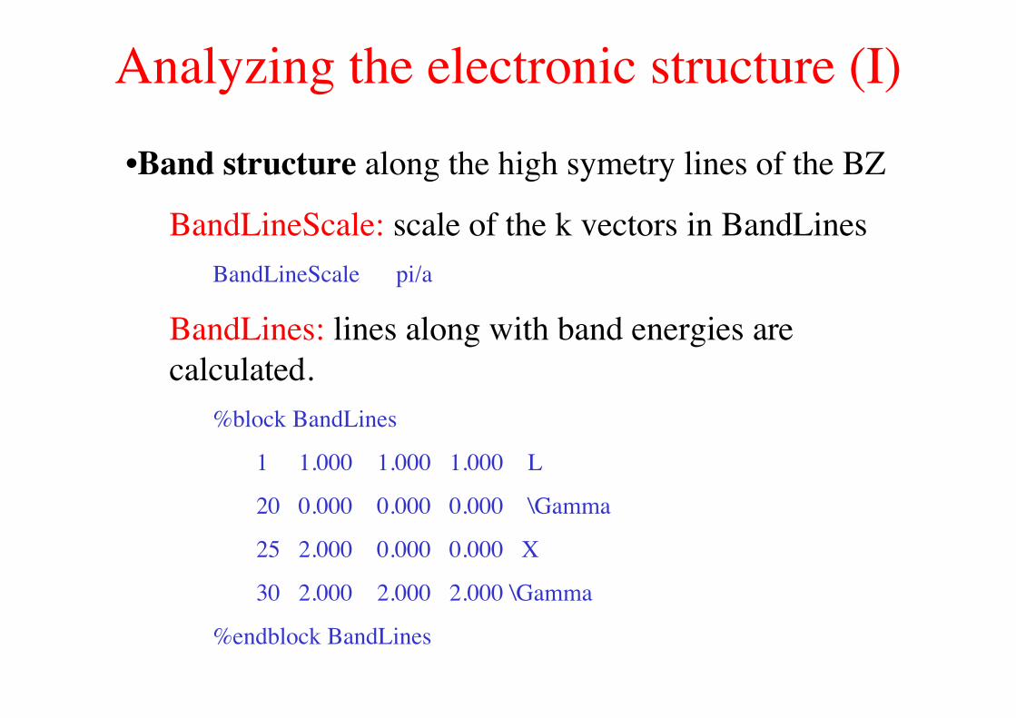
Analyzing the electronic structure (I)•Band structure along the high symetry lines of the BZ

BandLineScale: scale of the k vectors in BandLinesBandLineScale pi/a

BandLines: lines along with band energies arecalculated.

%block BandLines

1 1.000 1.000 1.000 L

20 0.000 0.000 0.000 \Gamma

25 2.000 0.000 0.000 X

30 2.000 2.000 2.000 \Gamma

%endblock BandLines

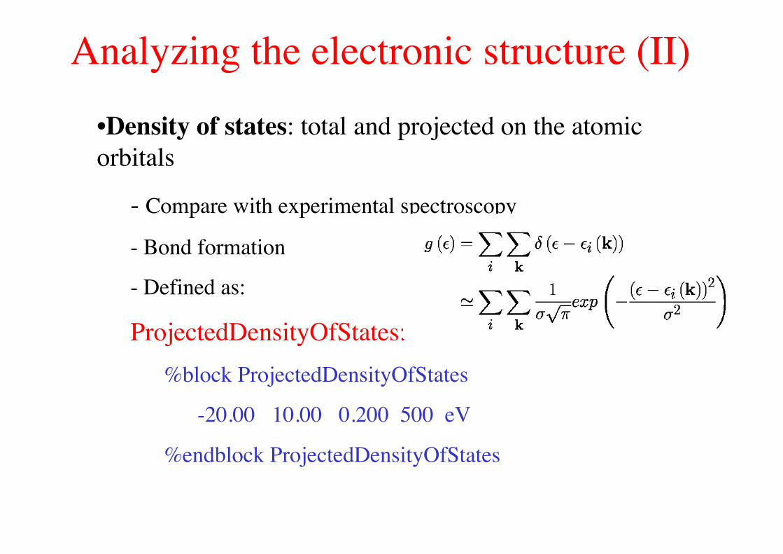
Analyzing the electronic structure (II)•Density of states: total and projected on the atomicorbitals

- Compare with experimental spectroscopy

- Bond formation

- Defined as:

ProjectedDensityOfStates:%block ProjectedDensityOfStates

-20.00 10.00 0.200 500 eV

%endblock ProjectedDensityOfStates

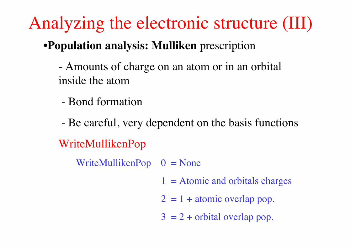
Analyzing the electronic structure (III)•Population analysis: Mulliken prescription

- Amounts of charge on an atom or in an orbitalinside the atom

- Bond formation

- Be careful, very dependent on the basis functions

WriteMullikenPop WriteMullikenPop 0 = None

1 = Atomic and orbitals charges

2 = 1 + atomic overlap pop.

3 = 2 + orbital overlap pop.

Tools (I)•Various post-processing programs:

-PHONONS:

-Finite differences: VIBRA (P. Ordejón)

-Linear response: LINRES ( J. M. Alons-Pruneda et al.)

-Interphase with Phonon program (Parlinsky)

-Visualize of the CHARGE DENSITY and POTENTIALS

-3D: PLRHO (J. M. Soler)

-2D: CONTOUR (E. Artacho)

-2D: DENCHAR (J. Junquera)

Tools (II)

-TRANSPORT PROPERTIES:

-TRANSIESTA (M. Brandbydge et al.)

-PSEUDOPOTENTIAL and BASIS information:

-PyAtom (A. García)

-ATOMIC COORDINATES:

-Sies2arc (J. Gale)