universitat politècnica de catalunya - iri · universitat politècnica de catalunya ... obstacle...

Universitat Politècnica de Catalunya

Master:

Automatic Control and Robotics

Master Thesis

Obstacle avoidance for mobile robotsusing lidar sensors

Juan Esteban Rodríguez Rosales

Director: Juan Andrade Cetto

Academic Course 2010/11

September 2011

Obstacle avoidance for mobile robots using lidar sensors 1

Abstract

This master thesis is aimed at developing a ROS compatible obstacle avoidance module

for a Segway RMP400 platform using lidar sensors. The algorithm implemented supports

different 3D scenarios, such as slopes and precipices. Given that the currently available

navigation modules in the ROS stack work only for 2D, significant modification of the

navigation stack was mandatory. The proposed solution does not take into account the

non-holonomic constraints of the platform. An alternative method is developed to tackle

this issue for the case of tele operated motion.

2 UNIVERSITAT POLITÈCNICA DE CATALUNYA

Index

Abstract 1

1 Introduction 7

2 Objectives 9

3 Related work 11

4 Design 17

4.1 Approach . . . . . . . . . . . . . . . . . . . . . . . . . . . . . . . . . . . . 17

4.2 Implementation . . . . . . . . . . . . . . . . . . . . . . . . . . . . . . . . . 19

4.2.1 From scans to point clouds . . . . . . . . . . . . . . . . . . . . . . . 19

4.2.2 From a 2D to a 3D representation of the world . . . . . . . . . . . . 20

4.2.3 Estimating the normals . . . . . . . . . . . . . . . . . . . . . . . . . 21

4.2.4 Concatenating point clouds . . . . . . . . . . . . . . . . . . . . . . 21

4.2.5 Avoiding obstacles . . . . . . . . . . . . . . . . . . . . . . . . . . . 22

4.3 Using the ROS navigation stack . . . . . . . . . . . . . . . . . . . . . . . . 23

4.4 Using teleoperation . . . . . . . . . . . . . . . . . . . . . . . . . . . . . . . 24

5 Experiments 25

5.1 Stairs . . . . . . . . . . . . . . . . . . . . . . . . . . . . . . . . . . . . . . . 26

5.2 Curb . . . . . . . . . . . . . . . . . . . . . . . . . . . . . . . . . . . . . . . 28

5.3 Static obstacles that can be surrounded . . . . . . . . . . . . . . . . . . . . 29

5.4 Cliff . . . . . . . . . . . . . . . . . . . . . . . . . . . . . . . . . . . . . . . 29

5.5 Slope . . . . . . . . . . . . . . . . . . . . . . . . . . . . . . . . . . . . . . . 31

5.5.1 Grass slope . . . . . . . . . . . . . . . . . . . . . . . . . . . . . . . 31

5.5.2 Soft slope . . . . . . . . . . . . . . . . . . . . . . . . . . . . . . . . 31

5.6 Mobile obstacles . . . . . . . . . . . . . . . . . . . . . . . . . . . . . . . . . 33

Conclusions 35

3


Future Work 35

Appendix A 37

Acknowledgments 45

Figure list

4.1 Point Cloud normal estimation . . . . . . . . . . . . . . . . . . . . . . . . 18

4.2 From scans to point clouds . . . . . . . . . . . . . . . . . . . . . . . . . . . 20

4.3 Clouder . . . . . . . . . . . . . . . . . . . . . . . . . . . . . . . . . . . . . 22

4.4 Zones for teleoperated navigation . . . . . . . . . . . . . . . . . . . . . . . 24

5.1 Comparison detection algorithm with data coming from a full 3D laser.

Left, the robot stays on a slope at a point A(see the stairs at point E,

and the departing ground region at point C). Right, the robot stays on the

horizontal ground. . . . . . . . . . . . . . . . . . . . . . . . . . . . . . . . . 26

5.2 Upward stairs. A) Scenario image, B) RVIZ visualization image . . . . . . 27

5.3 Curb. A) Scenario image, B) RVIZ visualization image. . . . . . . . . . . . 28

5.4 Tree. A) Scenario image, B) RVIZ visualization image . . . . . . . . . . . 29

5.5 Cliff. A) Scenario image, B) RVIZ visualization image . . . . . . . . . . . 30

5.6 Slopes. A) Grass slope scenario image, B) RVIZ soft slope visualization

image . . . . . . . . . . . . . . . . . . . . . . . . . . . . . . . . . . . . . . 32

7 Navigation Stack Overview . . . . . . . . . . . . . . . . . . . . . . . . . . . 41

8 IRI’s robot Teo . . . . . . . . . . . . . . . . . . . . . . . . . . . . . . . . . 43

5


1. Introduction

One of the most challenging aspects in autonomous outdoor mobile robot navigation

is reliability. That is, a mobile robot must me able to reach its destination safely, every

single time, not only avoiding collisions to obstacles and humans around it, but also

successfully driving through difficult paths such as slopes, bumps, or potholes.

Given a planed path formed by a set of waypoints, a low level navigation routine

should make the robot traverse from the departing node at a given kinematic constraint

(pose and speed) and reach the destination node also at a desired pose and speed.

During such navigation task from one intermediate waypoint to the next, sensor data

at high frame rate is analyzed in order to determine whether the path is traversable, or

whether an obstacle is found, and a countermeasure to the navigation commands must

be computed to safely clear the obstacle. This thesis pertains the computation of such

navigation commands.

Sensors that can be used for obstacle avoidance typically estimate the distance or time

to contact between the robot and the obstacles. These include:

• A belt of proximity sensors (ultrasound, infrared, etc).

• One or more lidar sensors at different orientations.

• A monocular or stereo vision system.


The choice of sensor modality depends on the environment and on the algorithms to be

used. For instance, infrared sensors are used only for small indoor robots, and sonar rings

are adequate for larger robots but also for indoor environments. Vision-based systems

are suitable for on-road outdoor navigation. But the use of pure vision systems is often

unreliable due to significantly varying illumination conditions. Laser-based systems are a

more robust alternative for outdoor off-road obstacle avoidance. The work presented here

uses this type of devices.

Many algorithmic solutions exist in the literature to solve the obstacle avoidance prob-

lem. Although most of them are designed for indoor scenarios, some implement strategies

to detect obstacles in 3D. Nevertheless, almost all of them lack the capability of navigating

in real 3D environments, clearing slopes or bumps, or avoiding stairs and cliffs.

In this master thesis, a 3D obstacle avoidance algorithm was devised, implemented and

tested using a Segway RMP400 robot, that is capable of traversing slopes and bumps,

and of avoiding stairs and cliffs.

This document summarizes our experiences conducting this research. Chapter 2 states

the objectives, framing the reach of our study. Related work is analyzed in chapter 3,

and our proposed method is developed in chapter 4. A mirage of experiments under very

different terrain conditions is presented in chapter 5. Conclusions and future work are

explained in the last two chapters. For readers with limited knowledge about the ROS

environment, a brief appendix is included. It also contains technical details about our

robot Teo.


2. Objectives

The objectives of this master thesis are:

• To implement a 3D ROS compatible obstacle avoidance method for a Segway RMP400.

• To be capable of using the system even with 2D odometry readings from the plat-

form.

• To implement and test the method within the current ROS Navigation Stack.

• To implement and test the method also under teleoperation of the platform using a

joystick.

• To extensively validate its use both indoors and outdoors with a Segway RMP400

mobile robot.


3. Related work

In this chapter, related work about obstacle avoidance is presented. Only some of

the most representative methods are analyzed, and conclusions are dawn to direct our

research.

The first step of any obstacle avoidance algorithm is to determine which part of the

environment is traversable, and which is an obstacle. This decision is carried out by

analyzing proprioceptive sensor data, and is obviously platform dependent. The most

typical approach is to discretize the space in front of the robot, either as a 2D plane, or in

3D, and label cells according to its traversability condition. One such method that uses

stereo vision for region segmentation is [7]. The procedure is divided in three steps:

First, a segmentation by region growing is performed. The output of this process is a

set of planar regions Pi with the following attributes; Pi = (ni, di, Ni, bi, Ai,Bi). Here ni

is the unit length normal vector of the plane, di the signed distance to the origin, Ni the

total number of points belonging to this plane, bi and Ai are the first two moments times

Ni , and Bi describes the region border which is represented as a vector of pairs where

each pair holds the start and end index of data points belonging to the plane for a given

scan line.


Using this information, a 3D occupancy grid is generated. Then, combining this

information with a floor map (i.e. x, y coordinates of the world around) the method

generates a floor obstacle grid (FOG). FOG : (x, y) → (t, h) where h is the cell number

and t one of the following types:

• floor: ever surface the robot can step on.

• stairs: small change in the floor height.

• border: large change in floor height.

• tunnel: low ceiling above the floor,

• obstacle: an obstacle the robot has to avoid,

• unknown: unclassified terrain.

The resulting representation classifies areas into one of six different types while also

providing object height information. This FOG is then fed to a robot controller to avoid

obstacles.

Once a reliable obstacle map is obtained one must come up with a method to navigate

around such obstacles, either reactively, following a predefined path, or both. A method

that propose a control law to such end is proposed in [8]. Despite being a 2D solution,

the method is defined as an obstacle avoidance navigation tool, and is based in the com-

bination of a nonlinear control law for path following coupled with a Deformable Virtual

Zone for obstacle avoidance.

The method consists in a guidance solution that embeds the path-following require-

ments in a desired proximity function (with respect to the obstacles) that drives the

robot to contour the obstacles while guaranteeing convergence on the path when there is

no obstacle.

The approach is based on the derivation of a Lyapunov function that guarantees

asymptotic convergence to the path without obstacles, and the boundedness of a variable


called the intrusion ratio, that captures the surrounding obstacles proximity and the

current robot situation with respect to the path.

Unfortunately, the kinematic model used and the kinematic control laws derived which

guarantee asymptotic convergence to the path (positive definiteness of the Lyapunov

function and negative semi definiteness of its derivative) are not easily extensible to the

3D case.

Obstacle avoidance from range data can be improved if sensor gaze can be controlled.

An interesting strategy to actively control sensor gaze is presented in [9]. In this case, a

3D obstacle avoidance method for mobile robots that uses a 2D laser range finder and a

ToF camera was proposed. To overcome the limited field of view of the sensor, the ToF

camera was mounted on the head of an anthropomorphic robot. This allows to change

the gaze direction through the robot head’s pan tilt and its torso yaw joint.

The method for obstacle detection is divided again in three steps: filtering, detection

of obstacle points and extraction of virtual scans. Filtering is done by detecting jump

edges when two points approximately lie along the line of sight of the camera. They

can be detected by examining local pixel neighborhoods. Secondly, a point pi,j is classi-

fied as belonging to an obstacle, if the difference between the maximum and minimum

height values in a local window around pi,j is above a minimum tolerable obstacle height

threshold.

At last, to create a virtual scan for each column of the ToF camera’s distance image,

the obstacle point with the shortest Euclidean distance to the robot is chosen. This

distance constitutes the range in the scan. If no obstacle point is detected in a column,

such scan point is marked invalid, giving it the maximum range of the sensor.

The resulting virtual scan of the scene is compared with the scan from the laser range

finder. For example, with a laser range finder, only the legs of a chair are detected, but,

when using the virtual scan, the whole contour of the chair is detected and added to the


occupancy grid.

Gaze control is directed by means of short temporal saccadic motions to the closest

objects to the robot. When no obstacles are present in the scene no saccades are executed

and the gaze is simple directed towards the forward looking direction of the robot.

Besides gaze control, another method to increase system performance is to use a

hierarchy of obstacle avoidance modules. In [10] for instance, two levels in the hierarchy

are proposed.

The first level is a dynamic hard stop which is designed to immediately stop the robot

if a large obstacle suddenly appears in its forward path at a close distance (< 2.5m). The

second level is reactive obstacle avoidance which modifies the follower path locally based

on a traversability map of obstacle free areas up to 5m away.

Using visual odometry, the hard stop obstacle detection algorithm fills in a ground

aligned Cartesian grid where each cell stores the height above ground for 3D points de-

tected at that location. It then aggregates the height statistics for each grid cell within

the designated area of interest (near robot, in its forward path) and applies thresholds for

acceptable sizes of obstacles after some noise removal.

Using this information, the hard stop module reports the presence of lethal obstacles

within the zone being monitored. The next level in the hierarchy determines the location

and severity of obstacles in a scene described by 3D range data. The range data is derived

from a real-time dense multi-resolution correlation based stereo algorithm and the camera

pose comes from the visual navigation solution. The algorithm produces an analog output

that measures obstacle severity (in terms of height, slope and size), so that subsequent

thresholding can determine which obstacles are considered to be traversable, based on

the characteristics of the vehicle. Frame-level obstacle maps are then stitched together,

in real-time, to form a local traversability map that is provided as input to path planning

module.


The algorithm proceeds as follows. The stereo range data is pre-filtered to reduce

noise and then transferred to Cartesian ground coordinates from image coordinates such

that ground resolution variation is accounted for. The data is then analyzed at multiple

resolutions to detect obstacles with varying slopes. The obstacle height is computed

from the heights of points on the obstacle boundary. The map representing these heights

is merged with the slope contribution to yield a traversability cost map. Finally, the

reactive path planner uses a time aggregated version of this map to navigate around

obstacles locally.

Related work conclusion

Our first conclusion is that regardless of the type of sensors used: lasers, stereo vision

or Time of Flight cameras, most methods resort to grid structures to locate obstacles in

the scene. Unfortunately, none of these techniques is reliable for the 3D navigation as

they will fail in regions with slopes or bumps. All of the above mentioned methods are

capable of detecting obstacles above or below the horizontal plane. Stairs and cliffs will

also be hard conditions for all of the methods studied.

Due to this, it is necessary to design a custom 3D navigation method that includes

a full 3D representation of the world, where the robot is capable of determining which

obstacles are traversable or not, taking into account scenarios in which the ground does

not follow a horizontal plane.


4. Design

In this chapter we will first explain how to detect and evade obstacles by analyzing

data from laser range finder streams and acting accordingly. Secondly, we will explain

how the method was implemented with the Teo robot using the ROS operating software.

4.1 Approach

In order to detect obstacles, the robot needs a 3D representation of the world around

it. By 3D representation, we mean a 3D point cloud that indicates where obstacles are,

i.e. walls, tables, people, etc. To classify the elements in a point cloud, a number of

computations need to be made on all points. For instance, to decide whether a region

local to each point in the cloud is a slope, floor, wall, or an object, we need to compute

curvature locally, as well as proximity to other points in the set. To this end, we compute,

for each point in the cloud, its normal vector, perpendicular to a local planar patch on

each point, and the Euclidean distance to its neighbors. See Figure Figure 4.1.

To fit normals to local planar patches we use a similar algorithm that the one presented

for segmentation of 3D urban mapping in [6]. Thus, considering each 3D point in the

dataset with coordinates p = (x, y, z)T , the error between a fitted planar patch and the


Figure 4.1: Point Cloud normal estimation

range map values for the kNNs to p is given by

ε =∑i∈K

(piTn− d)2,

where n = (nx, ny, nz)T is the local surface normal at p, K is the set of kNNs to p, and d

is the distance from p to the plane. This error can be re-expressed in the following form

ε = nT (∑i∈K

(pipiT ))︸︷︷︸

Q

n− 2d (∑i∈K

(piT ))︸︷︷︸

q

n+ |K|2d2.

Combining the above error metric with the orthonormality property for each local

surface normal into a Lagrangian of the form

l(nT , d, λ) = ε+ λ(1− nTn),

The local surface normal that best fits the patch K is the one that minimizes the above

expression. Deriving l with respect to n and d, and setting the derivatives to zero, it turns

out that the solution is the eigenvector asociated to the smallest eigenvalue of

(Q− qqT

|K|2)n = λn.


4.2 Implementation

First, we needed a device to measure 3D range data from the environment in the form

of point clouds. A Microsoft Kinect camera was the first option. This type of cameras

triangulate infrared modulated light to compute a 2D image of range data. We tested

the camera at both indoor and outdoor scenarios, testing different illumination cases and

several distances of obstacles to the camera. The results of these tests were that the

Kinect camera showed a reasonably good behavior at indoor scenarios, but not outdoors.

With severe sunlight exposure, the performance of the Kinect camera was poor, and thus

the sensor was unreliable for our purposes.

Our alternative was to use a Hokuyo laser range finder, which is more reliable both

indoors and outdoors. However, these lasers only return a single scan, indicating how far

from lasers there is anything in a semi-circle in front of them. Thus, we needed a software

module to aggregate single scans from the moving platform into a point cloud.

4.2.1 From scans to point clouds

In order to aggregate single laser scans into a 3D point cloud, we use a ROS Laser

Scan Assembler service. The laser assembler needs two parameters to work, the laser scan

topic and the output point cloud frame. Then, when a client requests a new point cloud

indicating a time interval, the laser assembler generates the point cloud using all scans

received inside that time interval.

The client used was a snapshotter. This module has a permanent trigger, that every

fixed number of seconds requests a cloud to the laser assembler. Then it publishes this

cloud as a new topic. This entire process (which is repeated at a determined frequency)

is shown in Figure 4.2.


Laser Assembler(ROS service)

Snapshotter(Client)

req res

Laser Scan TopicLaser Frame

Point Cloud TopicDesired Frame

Figure 4.2: From scans to point clouds

4.2.2 From a 2D to a 3D representation of the world

The robot platform Teo is an all-terrain vehicle designed for navigation in outdoor

scenarios, and specially in uneven terrains. However, the odometric data that can be

computed from the robot wheel encoders is essentially 2D. This produces undesired effects

in the treatment of the range data coming from its forward looking range sensors. For

instance, sensing the floor in front of the robot whilst entering and exiting a ramp will be

interpreted as obstacles appearing in front of the robot.

In order to fix this issue, our algorithm takes the pitch angle value from the segway’s

internal inertial measurement units, and uses it to transform the current scan, multiplying


by the rotation matrix below:

R =

cos θ 0 sin θ

0 1 0

− sin θ 0 cos θ

where θ is the current pitch angle.

4.2.3 Estimating the normals

The next step is to compute the local orientation of planar patches for each point in

the cloud. For this, we used the ROS Point Cloud Library.

Two criteria have been devised to select the set of neighbors to a point: by using a

fixed radius (i.e., all points inside a sphere centered on the query point are considered

neighbors), or by counting a fixed number of neighbors to a point. We choose the later

option in all of our experiments because by using a fixed radius is too computationally

expensive, forbidding real time.

The computation of the normals for the entire point cloud is an expensive computation

process. Therefore, our dense aggregated point clouds are first downsampled by a regular

grid. If more than one point is inside any cell, the filter only left one, eliminating the

others.

4.2.4 Concatenating point clouds

Now, each point cloud includes its normals, but this is not enough to make a good 3D

representation because they are small clouds (only a few laser scans). This is the reason

why we concatenate each new cloud with a predefined number of previous clouds. Thus,

a bigger point cloud allows a better representation of the world.


In our algorithm, either estimating the normals and concatenating point clouds is

performed by a new module, called Clouder. To concatenate point clouds, Clouder uses a

ROS Cloud Assembler service, with the same functioning of the laser assembler, but using

point clouds. Finally, Clouder publishes these bigger clouds in a new topic, as shown in

Figure 4.3.

Clouder

DownsamplingNormal

EstimationConcatenating

Topic Type:Point CloudDense: YesSize: Small

Topic Type:Point CloudDense: NoSize: Small

Topic Type Normal Point CloudDense: NoSize: Small

Topic Type Normal Point CloudDense: NoSize: Big

Figure 4.3: Clouder

4.2.5 Avoiding obstacles

Using this bigger cloud, the algorithm detects the obstacles around. First of all, one

can realize that the frame in which points will be checked is the base frame of the robot,

thus, value of z lower than zero means that the point is below the ground. Given that

points located below the z plane cannot be considered as obstacles (for example slopes),

all computations are made in absolute coordinates.

Then, if the component z of the normal is low, it means that the orientation of the

planar patch is heavily tilted away from the horizontal plane. In this case, the area might

belong to a wall, person or any other obstacle. On the other hand, if the value of z in

the normal to a point is medium or high, the point cloud is explored looking for points

lower than the point of interest, in a rectangle column (15 cms long and 5 cms width).

When finding one point that satisfies these conditions, all three normal components are


compared, if they are similar it indicates that both points belong to the same structure

(i.e. same wall, ground, etc). If this new point is close to z = 0, and its normal indicates

that belongs to a soft slope, it means that the robot can pass through those points, so

they will not be marked as obstacles.

In order to make the algorithm faster, points near to the ground are not studied,

because the kinematic properties of the robot are sufficient for it to overtake them. Also,

the algorithm takes into account the maximum possible height of the obstacles. This

means that if any obstacle is higher than that value, then it is not marked as obstacle.

Thus, the algorithm disregards those points that pass above the vehicle without collision.

4.3 Using the ROS navigation stack

When the robot knows where the obstacles are it can navigate without collision. Thus,

in this section we explain the changes done to adapt ROS Navigation Stack to our robot.

This task was a difficult one because the stack is a large software project and is not

optimally documented.

Since the stack does not make use of local orientation to each point in the cloud.

Passing the newly created data structure to the module was unnecessary. The first change

was to strip down the point cloud from its normals and pass it in the requested data type.

The ROS navigation stack computes a costmap. That is, a small grid in front of the

robot in which each cell is given a value that determines the capability of the robot for

passing thru it. Cells with obstacles have a low traversability value in the cost map,

whereas free space has higher traversability. Obviously, determining the costmap was

the module that more changes suffered. Instead of using the detecting obstacle method

implemented by ROS developers, our algorithm was implemented.

Nevertheless, for navigation purposes, we decided to stick to the 2D costmap from our


3D representation. This does not affect robot navigation, because the robot movements

are locally constrained to a plane.

4.4 Using teleoperation

This navigation method was implemented for to guide the robot with a joystick. The

algorithm takes into account the current velocity of the robot and a the input clouds,

then this method is capable of determining if the robot may collide with any obstacle.

Instead of using a costmap as in the ROS Navigation Stack, this method defines six

parameterized zones in front of the robot, as shown in Figure 4.4.

TEO

ZONE F

ZONE E

ZONE D

ZONE C

ZONE B

ZONE A

x

y

Figure 4.4: Zones for teleoperated navigation

If any obstacle is detected, depending on its position, the algorithm forbids velocities

that conduce to collision. For example, if the obstacle is in Zone E, only backward or in

place rotation velocities are allowed, if these are in Zone C, high translational velocities

and soft left turns are forbidden. For those cases, the robot will stop until it receives a

new allowed velocity command or the obstacle disappears.


5. Experiments

One of the most important steps during the development phase was the testing and

validation of the various software modules developed during the project. In our case, the

first required validation is the one that concerns to obstacle detection algorithm. In order

to achieve this, we compared our results with those of a 3D laser that represents perfectly

the world around the vehicle.

Figure 5.1 shows the result of applying our algorithm to a scenario with several obsta-

cles. In such scenario, the algorithm only detects as obstacles those points that the robot

can not overtake, which are marked in red. On the other hand, green points represent

traversable points. In the Figure, A is robot itself, B is a person, C is a slope (on left

image, Teo stays on a slope, so the horizontal ground is seen as a slope by the robot), D

are trees, E are stairs with edge and F is a wall. On left image, Teo stays on a slope, then,

it moves forward, until it stays on the horizontal ground, as seen on the right image.

Given the low density of leafs and branches on trees and bushes, parts of these are

marked as traversable space. This is not a problem because, the rest of the plant is still

marked as obstacle, which is sufficient to avoid collision.

Once the obstacle detection algorithm was validated, the next set of experiments


B

A

C

D

E

D

B

A

CDE

F

Figure 5.1: Comparison detection algorithm with data coming from a full 3D laser. Left,

the robot stays on a slope at a point A(see the stairs at point E, and the departing ground

region at point C). Right, the robot stays on the horizontal ground.

was intended to test algorithm behavior within ROS navigation stack and also during

teleoperated navigation. A number of scenarios is chosen that represent prototypical

situations for the Teo robot, a vehicle designed to navigate in human pedestrian areas.

First, the scenario of interest is introduced, where the robot always starts a few meters far

from the obstacles. Then the robot is directed towards the obstacle, and data is gathered.

We present the results of using both the ROS Navigation Stack and the teleoperated

navigation. When using the ROS stack, the goal pose is defined behind the obstacle. On

the other hand, during teleoperated navigation, we used a joystick to guide the robot.

5.1 Stairs

In the first test Teo is facing a set of upward stairs, as shown at the left of Figure

5.2, in which Teo is moving straight ahead to the stairs. At the right, the image shows

rviz visualization, where the red arrow marks the goal pose, the green dots belongs to the


point cloud generated with the floor laser scans, the front laser is marked in white, red

points are obstacles and inflated obstacle space (i.e the robot’s center can not stay in this

zone). The robot is denoted by its frames. As it can be seen, both the front laser and

floor laser detect the step as obstacle.

A B

Figure 5.2: Upward stairs. A) Scenario image, B) RVIZ visualization image

Navigation Method Result

ROS Navigation Stack When it realizes that there is an obstacle to collide

with, it looks for an alternative path, moving around

the stairs. Depending on the configuration of the stack,

the robot reacts on different ways. In our case, after

a few meters, the robot stops, waiting for a new goal,

because it is not capable of find a path without obsta-

cles. For example, other configurable behavior is that

the robot continues searching a new path indefinitely..

Teleoperated When the robot detects the stairs, it stops, waiting for

a new velocity command that avoids collision.


5.2 Curb

This test shows algorithm response when the robot is facing a curb, either going up

or down. In this case, depending on the height of the curb two behaviors are expected. If

Teo is capable of overtaking the curb, this will not be marked as obstacle, so the robot will

be able to pass through it. Otherwise, if the curb is big, it will be treated like any other

obstacle. A typical curb is shown in Figure 5.3. In our experiments, the curb used is big

enough to be marked as an obstacle. As shown in the image to the right, the downlooking

front laser detects a jump edge a few centimeters below the ground floor (green dots), so

the algorithm is able to detect the step as an obstacle, as indicated by the red and orange

marks.

A B

Figure 5.3: Curb. A) Scenario image, B) RVIZ visualization image.


ROS Navigation Stack Again, the robot tries to surround the obstacle unsuc-

cessfully. Teo stops and waits for a new goal. This

behavior is repeated either going up and going down.

Teleoperated Again, the curb is marked as an obstacle, so Teo stops

and waits for a new velocity command.


5.3 Static obstacles that can be surrounded

By Static obstacles we mean those obstacles that are easily surrounded, such obstacles

are tables, benches, trees, etc. For example, in Figure 5.4 a tree is shown. In these cases,

the expected behavior is that Teo marks them as obstacles.

A B

Figure 5.4: Tree. A) Scenario image, B) RVIZ visualization image


ROS Navigation Stack In this case, Teo is capable of surrounding the tree,

reaching the goal. It avoids the obstacle with no prob-

lem.

Teleoperated Teo stops and waits for a new velocity to avoid collision.

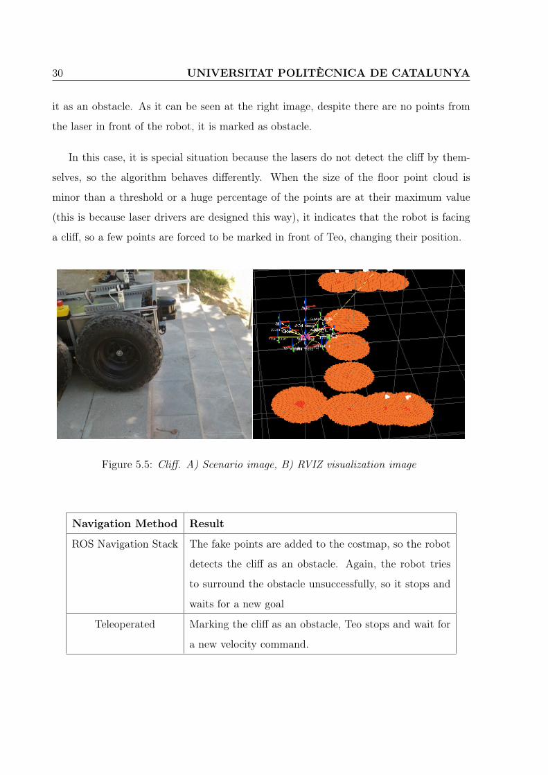
5.4 Cliff

This scenario is a representation of stairs when going down, either indoor or outdoor.

An example is shown in Figure 5.5. Obviously, the expected behavior is that Teo marks


it as an obstacle. As it can be seen at the right image, despite there are no points from

the laser in front of the robot, it is marked as obstacle.

In this case, it is special situation because the lasers do not detect the cliff by them-

selves, so the algorithm behaves differently. When the size of the floor point cloud is

minor than a threshold or a huge percentage of the points are at their maximum value

(this is because laser drivers are designed this way), it indicates that the robot is facing

a cliff, so a few points are forced to be marked in front of Teo, changing their position.

A B

Figure 5.5: Cliff. A) Scenario image, B) RVIZ visualization image


ROS Navigation Stack The fake points are added to the costmap, so the robot

detects the cliff as an obstacle. Again, the robot tries

to surround the obstacle unsuccessfully, so it stops and

waits for a new goal

Teleoperated Marking the cliff as an obstacle, Teo stops and wait for

a new velocity command.


5.5 Slope

This test is aimed to show how Teo behaves when facing slopes. In order to test this,

two slopes were tested. The first of them is a big irregular slope, and the second one

is a soft regular slope. The slopes used are shown in Figure 5.6. The left image shows

a big grass slope and the right image shows rviz visualization of a soft slope seen from

the side. In this case, the floor point cloud (green dots) is not cleared out because we

intend to show what happens in this scenario. Thus, the point cloud should represent the

horizontal ground, then an up slope and finally a horizontal ground again. Nevertheless,

when the Teo’s status changes (i.e. goes from horizontal to inclined or viceversa), it does

not represent well the ground, and the robot sees an imaginary step as shown at the right

image. This issue also occurs when taking into account the pitch angle status. Although

using this pitch status improves the representation, it is not enough to achieve a perfect

representation of the world. Due to this, Teo detects an imaginary step, so it sees an

obstacle.

5.5.1 Grass slope

Although this is a big slope, Teo is capable of overtaking it, so the expected behavior

is that the slope will not be marked as an obstacle.

5.5.2 Soft slope

As an example, a disabled people slope was used to test Teo behavior. Being a soft

slope, the robot is capable of going through it, so the expected behavior is that Teo will

not marked the slope as obstacle.


A B

Figure 5.6: Slopes. A) Grass slope scenario image, B) RVIZ soft slope visualization image


ROS Navigation Stack Due to ground irregularities and the large steepness of

the slope, the ROS Navigation Stack marks the slope as

obstacle but, when Teo gets closer looking for an alterna-

tive path, it realizes that there is no obstacle, so finally

overtakes the slope. When Teo is going down, given that

it is a very steep slope, the downward looking floor laser

does not detect it, so unfortunately is marked as a cliff.

Teleoperated Using teleoperated Navigation, when marking as obsta-

cle the slope, Teo stops, so it is not capable of overtake

it. Again, when Teo is going down, the floor laser does

not detect the slope, so it is marked as a cliff.



ROS Navigation Stack Due to Teo detects an imaginary step, it stops less than

a second until the step disappears, so the robot realizes

that there is no obstacle, and finally overtakes the slope.

Teleoperated The robot behavior in this case is the same, first it stops

less than a second, and then it continues moving.

5.6 Mobile obstacles

People are the most common mobile obstacles that the robot can collide with, so this

test intends to probe how Teo reacts to these obstacles. The expected behavior is that,

if the obstacle does not disappear, both methods react avoiding collision. On the other

hand, if the obstacle disappears, the robot must continue its movement.

Due to the people is first detected by the front laser, they can walk at a normal

velocity being detected by the robot without collision. If the person is running (or the

mobile obstacle is fast) at a few meters by second, collision may occur.


ROS Navigation Stack The robot will change its path avoiding collision. If

the obstacle disappears before the robot gets closer, the

costmap will be cleared, so no change happens.

Teleoperated The robot stops until it receives a new velocity command

or the obstacle disappears.


Conclusions

In this work we have implemented a navigation method that builds a 3D representation

of the world.

Our algorithm is modular, integrated with the ROS environment and takes as input

a point cloud. Thus, it could also work for other ROS-enabled robots and sensors, such

as a ToF camera or dense stereo data from images.

But, as we explained before, the obstacle detection algorithm works fine when a perfect

representation of the world around is achieved. This means that the robot perfectly knows

its local position in the world. Nevertheless, we did not achieve this perfect representation

in this Master Thesis, because our algorithm designed to generate the aggregated point

cloud is dependent of accurate 3D robot odometry. As it stands today, the odometry of

the robot is only 2D and using the pitch angle did not completely fix this issue. Although,

sufficient improvement in the world representation was achieved to successfully finalize

the proposed experimental benchmarks.

Even when using the current ROS navigation stack the method did not work perfectly

(i.e. Teo is not capable of making long curved trajectories), some 3D navigation was

achieved. Using the teleoperated navigation allowed faster tests and use of our algorithm

in those cases in which the ROS navigation stack failed.


Future work

Even when modest obstacle avoidance was possible for outdoor environments, reliable

3D navigation in all conditions is still down the road. As a result of the experience gained

in the realization of this project, these are our suggestions for future research to improve

the results of the method. For example, improve the navigation stack for non-holonomic

vehicles. Also, the implementation of 3D Time of Flight camera instead of lasers to avoid

the need to aggregate a point cloud.


Appendix A

In this appendix, we describe the tools that we used in this research. First, the

integrated software environment in which it was developed. Secondly, we present the

robot used to implement our algorithm.

Robot Operating System (ROS)

ROS is an open-source, meta-operating system for any robot. It provides the services

expected from an operating system, including hardware abstraction, low-level device con-

trol, implementation of commonly-used functionality, message-passing between processes,

and package management. It also provides tools and libraries for obtaining, building,

writing, and running code across multiple computers. The ROS runtime "graph" is a

peer-to-peer network of processes that are loosely coupled using the ROS communication

infrastructure. ROS implements several different styles of communication, including syn-

chronous RPC-style communication over services, asynchronous streaming of data over

topics, and storage of data on a Parameter Server.


ROS Filesystem Level

The filesystem level concepts are ROS resources that it may be encounter on disk,

such as:

• Packages: Packages are the main unit for organizing software in ROS. A package

may contain ROS runtime processes (nodes), a ROS-dependent library, datasets,

configuration files, or anything else that is usefully organized together.

• Stacks: Stacks are collections of packages that provide aggregate functionality,

such as a "navigation stack." Stacks are also how ROS software is released and have

associated version numbers.

• Message (msg) types: Message descriptions, define the data structures for mes-

sages sent in ROS.

• Service (srv) types: Service descriptions, define the request and response data

structures for services in ROS.

ROS Computation Graph Level

The Computation Graph is the peer-to-peer network of ROS processes that are pro-

cessing data together. The basic Computation Graph concepts of ROS are nodes, Master,

Parameter Server, messages, services, topics, and bags, all of which provide data to the

Graph in different ways.

• Nodes: Nodes are processes that perform computation. ROS is designed to be

modular at a fine-grained scale; a robot control system will usually comprise many

nodes. For example, one node controls a laser range-finder, one node controls the

wheel motors, one node performs localization, one node performs path planning,

etc.


• Master: The ROS Master provides name registration and lookup to the rest of the

Computation Graph. Without the Master, nodes would not be able to find each

other, exchange messages, or invoke services.

• Parameter Server: The Parameter Server allows data to be stored by key in a

central location. It is currently part of the Master.

• Messages: Nodes communicate with each other by passing messages. A message

is a simply a data structure, comprising typed fields.

• Topics: Messages are routed via a transport system with publish/subscribe seman-

tics. A node sends out a message by publishing it to a given topic. The topic is a

name that is used to identify the content of the message.There may be multiple con-

current publishers and subscribers for a single topic, and a single node may publish

and/or subscribe to multiple topics.

• Services: The publish/subscribe model is a very flexible communication paradigm,

but its many-to-many, one-way transport is not appropriate for request/reply inter-

actions, which are often required in a distributed system. Request/reply is done via

services, which are defined by a pair of message structures: one for the request and

one for the reply.

Nodes connect to other nodes directly; the Master only provides lookup information,

much like a DNS server. Nodes that subscribe to a topic will request connections from

nodes that publish that topic, and will establish that connection over an agreed upon

connection protocol. The most common protocol used in a ROS is called TCPROS,

which uses standard TCP/IP sockets.


Navigation Stack

Navigation is a ROS stack that takes in information from odometry, sensor streams,

and a goal pose and outputs safe velocity commands that are sent to a mobile base. At

the moment, it is only a 2D navigation stack.

Although this stacks groups several packages, the most important ones used in this

Master Thesis are:

• move_base: The move_base package provides an implementation of an action

that, given a goal in the world, will attempt to reach it with a mobile base. The

move_base node links together a global and local planner to accomplish its global

navigation task.

• nav_core: This package provides common interfaces for navigation specific robot

actions. Currently, this package provides the BaseGlobalPlanner, BaseLocalPlan-

ner, and RecoveryBehavior interfaces, which can be used to build actions that can

easily swap their planner, local controller, or recovery behavior for new versions

adhering to the same interface.

• base_local_planner/dwa_local_planner: This package provides implemen-

tations of the Trajectory Rollout and Dynamic Window approaches to local robot

navigation on a plane. Given a plan to follow and a costmap, the controller produces

velocity commands to send to a mobile base.

• costmap_2d: This package provides an implementation of a 2D costmap that

takes in sensor data from the world, builds a 2D or 3D occupancy grid of the data

(depending on whether a voxel based implementation is used), and inflates costs in

a 2D costmap based on the occupancy grid and a user specified inflation radius.

• voxel_grid: provides an implementation of an efficient 3D voxel grid. The occu-

pancy grid can support 3 different representations for the state of a cell: marked,


free, or unknown.

Using this packages, the navigation stack is capable to lead the mobile base to a

determined goal. In Figure 7 a conceptual overview of the navigation stack is shown.

This figure shows how it works, what topics and their types are needed to accomplish a

successful navigation.

The sensor transform node indicates relationships between different used frames, for

example, between sensor frames and the robot base frame. This node is necessary to trans-

form input scans from sensor sources. Using those sensor scans, both the global_costmap

and the local_costmap are updated. If there is any new obstacle it is added to the

costmaps. In case that current global or local planned path will guide the robot to collide,

both paths are modified, so new velocities are sent to mobile base. Recovery_behaviors

may optionally perform alternative behaviors when the robot perceives itself as stuck.

Figure 7: Navigation Stack Overview


Teo Robot

Teo is a robot designed at the Institut de Robòtic a i Informàtica Industrial, a Joint

Research Center of the Technical University of Catalonia (UPC) and the Spanish Council

for Scientific Research (CSIC).

This robot is a mobile robot based on a Segway RMP400, and is made of two Segway

units rigidly attached in a skid steer configurations. That is, Teo is a non-holonomic

robot.

Components

With a server computer and a router, both wifi and ethernet communications are

possible. Also, it has many sensors to infer about with the world around it. The principal

components are:

• Processing:

Arbor FPC7300 - Rugged Industrial PC

• Communications:

Router D-Link DIR-825

Switch D-Link DES-1005D

Bluetooth dongle Trust 16008

• Sensors:

PointGrey Flea Cameras (2)

Hokuyo lasers (3)

Septentrio AstRx1 GPS with antenna


TCM3 Compass

H3D laser (3D laser)

• Power:

VI-J41-EW-B1 Conversor 74..12V

SDS-035A-05 Conversor 12..5V

• Other:

Viper S4 Emergency Remote Relay

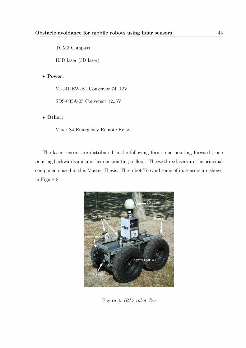
The laser sensors are distributed in the following form: one pointing forward , one

pointing backwards and another one pointing to floor. Theese three lasers are the principal

components used in this Master Thesis. The robot Teo and some of its sensors are shown

in Figure 8.

3D Laser

Flea Cameras

Front Laser

Floor Laser

Rear Laser

Segway RMP 400

Figure 8: IRI’s robot Teo


Teo & ROS

Teo’s ROS packages and drivers are developed at IRI.


Acknowledgements

To the wolf pack. Without them I would have abandoned this master after a few

months probably. They did not give me either strength, motivation or anything else.

They just stayed beside me, and we supported each other and kept walking, always

forward.

Bibliography

[1] Sebastian Thrun, Wolfram Burgard and Dieter Fox, Probabilistic Robotics, The MIT

Press, September 2005.

[2] Gregory Dudek and Michael Jenkin, Computational Principles of Mobile Robotics,

Cambridge University Press, July 2010.

[3] Willow Garage, Robot Operating System, www.ros.org, consulted February-August

2011.

[4] Willow Garage, NVidia, Google, and Toyota, Point Cloud Library,

www.pointclouds.org, consulted February-August 2011.

[5] Institut de Robòtica i Informàtica Industrial, Universitat Politècnica de Catalunya,

Teo Robot,www.wikiri.upc.es, consulted February-August 2011.

[6] Agustín Ortega, Ismael Haddad and Juan Andrade-Cetto, Graph-based Segmentation

of Range Data with Applications to 3D Urban Mapping, In Proc. of European Confer-

ence on Mobile Robots, 23-25 September 2009, Mlini/Dubrovnik, Croatia, pp. 193-198

[7] Jens-Steffen Gutmann, Masaki Fukuchi and Masahiro Fujita, 3D Perception and En-

vironment Map Generation for Humanoid Robot Navigation, International Journal of

Robotics Research, Vol. 27, No. 10, October 2008, pp. 1117-1134.

47


[8] Lionel Lapierre, Rene Zapata and Pascal Lepinay, Combined Path-following and Obsta-

cle Avoidance Control of a Wheeled Robot, International Journal of Robotics Research,

Vol. 26, No. 4, April 2007, pp. 361-375.

[9] David Droeschel, Dirk Holz, Jörg Stückler and Sven Behnke, Using Time-of-Flight

Cameras with Active Gaze Control for 3D Collision Avoidance. In Proc. of IEEE

International Conference on Robotics and Automation, pp. 4035-4040, 3-7 May 2010,

Anchorage, Alaska, USA.

[10] Aveek Das, Oleg Naroditsky, Zhiwei Zhu, Supun Samarasekera and Rakesh Kumar,

Robust Visual Path Following for Heterogeneous Mobile Platforms, In Proc. of IEEE

International Conference on Robotics and Automation, pp. 2431-2437, 3-7 May 2010,

Anchorage, Alaska, USA.

universitat politècnica de catalunya - iri · universitat politècnica de catalunya ... obstacle...

Documents