université de montréal deep learning of representations and its
TRANSCRIPT
Universite de Montreal
Deep learning of representations and its application to computer vision
par Ian Goodfellow
Departement d’informatique et de recherche operationnelleFaculte des arts et des sciences
These presentee a la Faculte des arts et des sciencesen vue de l’obtention du grade de Philosophiæ Doctor (Ph.D.)
en informatique
Avril, 2014
c� Ian Goodfellow, 2014.
Résumé
L’objectif de cette these par articles est de presenter modestement quelquesetapes du parcours qui menera (on espere) a une solution generale du probleme del’intelligence artificielle. Cette these contient quatre articles qui presentent chacunune di↵erente nouvelle methode d’inference perceptive en utilisant l’apprentissagemachine et, plus particulierement, les reseaux neuronaux profonds. Chacun de cesdocuments met en evidence l’utilite de sa methode proposee dans le cadre d’unetache de vision par ordinateur. Ces methodes sont applicables dans un contexteplus general, et dans certains cas elles ont ete appliquees ailleurs, mais ceci ne serapas aborde dans le contexte de cette de these.
Dans le premier article, nous presentons deux nouveaux algorithmes d’inferencevariationelle pour le modele generatif d’images appele codage parcimonieux “spike-and-slab” (CPSS). Ces methodes d’inference plus rapides nous permettent d’utiliserdes modeles CPSS de tailles beaucoup plus grandes qu’auparavant. Nous demon-trons qu’elles sont meilleures pour extraire des detecteur de caracteristiques quandtres peu d’exemples etiquetes sont disponibles pour l’entraınement. Partant d’unmodele CPSS, nous construisons ensuite une architecture profonde, la machine deBoltzmann profonde partiellement dirigee (MBP-PD). Ce modele a ete concu demaniere a simplifier d’entraınement des machines de Boltzmann profondes qui ne-cessitent normalement une phase de pre-entraınement glouton pour chaque couche.Ce probleme est regle dans une certaine mesure, mais le cout d’inference dans lenouveau modele est relativement trop eleve pour permettre de l’utiliser de manierepratique.
Dans le deuxieme article, nous revenons au probleme d’entraınement joint demachines de Boltzmann profondes. Cette fois, au lieu de changer de famille demodeles, nous introduisons un nouveau critere d’entraınement qui donne naissanceaux machines de Boltzmann profondes a multiples predictions (MBP-MP). LesMBP-MP sont entraınables en une seule etape et ont un meilleur taux de succesen classification que les MBP classiques. Elles s’entraınent aussi avec des methodesvariationelles standard au lieu de necessiter un classificateur discriminant pour ob-tenir un bon taux de succes en classification. Par contre, un des inconvenients detels modeles est leur incapacite de generer des echantillons, mais ceci n’est pas tropgrave puisque la performance de classification des machines de Boltzmann pro-fondes n’est plus une priorite etant donne les dernieres avancees en apprentissagesupervise. Malgre cela, les MBP-MP demeurent interessantes parce qu’elles sont ca-pable d’accomplir certaines taches que des modeles purement supervises ne peuventpas faire, telles que celle de classifier des donnees incompletes ou encore celle decombler intelligemment l’information manquante dans ces donnees incompletes.
ii
Le travail presente dans cette these s’est deroule au milieu d’une periode detransformations importantes du domaine de l’apprentissage a reseaux neuronauxprofonds qui a ete declenchee par la decouverte de l’algorithme de “dropout” parGeo↵rey Hinton. Dropout rend possible un entraınement purement supervise d’ar-chitectures de propagation unidirectionnel sans etre expose au danger de sur-entraınement. Le troisieme article presente dans cette these introduit une nouvellefonction d’activation specialement concue pour aller avec l’algorithme de Dropout.Cette fonction d’activation, appelee maxout, permet l’utilisation de aggregationmulti-canal dans un contexte d’apprentissage purement supervise. Nous demon-trons comment plusieurs taches de reconnaissance d’objets sont mieux accompliespar l’utilisation de maxout.
Pour terminer, sont presentons un vrai cas d’utilisation dans l’industrie pour latranscription d’adresses de maisons a plusieurs chi↵res. En combinant maxout avecune nouvelle sorte de couche de sortie pour des reseaux neuronaux de convolution,nous demontrons qu’il est possible d’atteindre un taux de succes comparable a celuides humains sur un ensemble de donnees coriace constitue de photos prises par lesvoitures de Google. Ce systeme a ete deploye avec succes chez Google pour lireenviron cent million d’adresses de maisons.
Mots-cles: reseau de neurones, apprentissage profond, apprentissage non su-pervise, apprentissage supervise, apprentissage semi-supervise, machines de Boltz-mann, les modeles bases sur l’energie, l’inference variationnel, l’apprentissage va-riationnel, le codage parcimonieux, reseaux neuronaux de convolution, la fonctiond’activation, “dropout,” la reconnaissance d’objets, transcription, reconnaissanceoptique de caracteres, geocodage, entrees manquantes
iii
Summary
The goal of this thesis is to present a few small steps along the road to solvinggeneral artificial intelligence. This is a thesis by articles containing four articles.Each of these articles presents a new method for performing perceptual inferenceusing machine learning and deep architectures. Each of these papers demonstratesthe utility of the proposed method in the context of a computer vision task. Themethods are more generally applicable and in some cases have been applied to otherkinds of tasks, but this thesis does not explore such applications.
In the first article, we present two fast new variational inference algorithmsfor a generative model of images known as spike-and-slab sparse coding (S3C).These faster inference algorithms allow us to scale spike-and-slab sparse coding tounprecedented problem sizes and show that it is a superior feature extractor forobject recognition tasks when very few labeled examples are available. We thenbuild a new deep architecture, the partially-directed deep Boltzmann machine (PD-DBM) on top of the S3C model. This model was designed to simplify the trainingprocedure for deep Boltzmann machines, which previously required a greedy layer-wise pretraining procedure. This model partially succeeds at solving this problem,but the cost of inference in the new model is high enough that it makes scaling themodel to serious applications di�cult.
In the second article, we revisit the problem of jointly training deep Boltz-mann machines. This time, rather than changing the model family, we present anew training criterion, resulting in multi-prediction deep Boltzmann machines (MP-DBMs). MP-DBMs may be trained in a single stage and obtain better classificationaccuracy than traditional DBMs. They also are able to classify well using standardvariational inference techniques, rather than requiring a separate, specialized, dis-criminatively trained classifier to obtain good classification performance. However,this comes at the cost of the model not being able to generate good samples. Theclassification performance of deep Boltzmann machines is no longer especially inter-esting following recent advances in supervised learning, but the MP-DBM remainsinteresting because it can perform tasks that purely supervised models cannot, suchas classification in the presence of missing inputs and imputation of missing inputs.
The general zeitgeist of deep learning research changed dramatically during themidst of the work on this thesis with the introduction of Geo↵rey Hinton’s dropoutalgorithm. Dropout permits purely supervised training of feedforward architectureswith little overfitting. The third paper in this thesis presents a new activationfunction for feedforward neural networks which was explicitly designed to workwell with dropout. This activation function, called maxout, makes it possible tolearn architectures that leverage the benefits of cross-channel pooling in a purely
iv
supervised manner. We demonstrate improvements on several object recognitiontasks using this activation function.
Finally, we solve a real world task: transcription of photos of multi-digit housenumbers for geo-coding. Using maxout units and a new kind of output layer forconvolutional neural networks, we demonstrate human level accuracy (with limitedcoverage) on a challenging real-world dataset. This system has been deployed atGoogle and successfully used to transcribe nearly 100 million house numbers.
Keywords: neural network, deep learning, unsupervised learning, supervisedlearning, semi-supervised learning, Boltzmann machines, energy-based models, vari-ational inference, variational learning, feature learning, sparse coding, convolutionalnetworks, activation function, dropout, pooling, object recognition, transcription,optical character recognition, inpainting, missing inputs
v
Contents
Resume . . . . . . . . . . . . . . . . . . . . . . . . . . . . . . . . . . . . ii
Summary . . . . . . . . . . . . . . . . . . . . . . . . . . . . . . . . . . . iv
Contents . . . . . . . . . . . . . . . . . . . . . . . . . . . . . . . . . . . vi
List of Figures . . . . . . . . . . . . . . . . . . . . . . . . . . . . . . . . x
List of Tables . . . . . . . . . . . . . . . . . . . . . . . . . . . . . . . . xii
1 Machine Learning . . . . . . . . . . . . . . . . . . . . . . . . . . . . . 11.1 Introduction to Machine Learning . . . . . . . . . . . . . . . . . . . 1
1.1.1 Generalization and the IID assumptions . . . . . . . . . . . 31.1.2 Maximum likelihood estimation . . . . . . . . . . . . . . . . 41.1.3 Optimization . . . . . . . . . . . . . . . . . . . . . . . . . . 5
1.2 Supervised learning . . . . . . . . . . . . . . . . . . . . . . . . . . . 81.2.1 Support vector machines and statistical learning theory . . . 9
1.3 Unsupervised learning . . . . . . . . . . . . . . . . . . . . . . . . . 111.4 Feature learning . . . . . . . . . . . . . . . . . . . . . . . . . . . . . 12
2 Structured Probabilistic Models . . . . . . . . . . . . . . . . . . . . 172.1 Directed models . . . . . . . . . . . . . . . . . . . . . . . . . . . . . 172.2 Undirected models . . . . . . . . . . . . . . . . . . . . . . . . . . . 18
2.2.1 Sampling . . . . . . . . . . . . . . . . . . . . . . . . . . . . 202.3 Latent variables . . . . . . . . . . . . . . . . . . . . . . . . . . . . . 21
2.3.1 Latent variables versus structure learning . . . . . . . . . . . 212.3.2 Latent variables for feature learning . . . . . . . . . . . . . . 22
2.4 Stochastic approximations to maximum likelihood . . . . . . . . . . 232.4.1 Example: The restricted Boltzmann machine . . . . . . . . . 25
2.5 Variational approximations . . . . . . . . . . . . . . . . . . . . . . . 262.5.1 Variational learning . . . . . . . . . . . . . . . . . . . . . . . 272.5.2 Variational inference . . . . . . . . . . . . . . . . . . . . . . 28
vi
2.6 Combining approximations: The deep Boltzmann machine . . . . . 29
3 Supervised deep learning . . . . . . . . . . . . . . . . . . . . . . . . . 31
4 Prologue to First Article . . . . . . . . . . . . . . . . . . . . . . . . . 364.1 Article Details . . . . . . . . . . . . . . . . . . . . . . . . . . . . . . 364.2 Context . . . . . . . . . . . . . . . . . . . . . . . . . . . . . . . . . 364.3 Contributions . . . . . . . . . . . . . . . . . . . . . . . . . . . . . . 374.4 Recent Developments . . . . . . . . . . . . . . . . . . . . . . . . . . 38
5 Scaling up Spike-and-Slab Models for Unsupervised Feature Learn-ing . . . . . . . . . . . . . . . . . . . . . . . . . . . . . . . . . . . . . . . 395.1 Introduction . . . . . . . . . . . . . . . . . . . . . . . . . . . . . . . 395.2 Models . . . . . . . . . . . . . . . . . . . . . . . . . . . . . . . . . . 42
5.2.1 The spike-and-slab sparse coding model . . . . . . . . . . . . 425.2.2 The partially directed deep Boltzmann machine model . . . 42
5.3 Learning procedures . . . . . . . . . . . . . . . . . . . . . . . . . . 455.3.1 Avoiding greedy pretraining . . . . . . . . . . . . . . . . . . 46
5.4 Inference procedures . . . . . . . . . . . . . . . . . . . . . . . . . . 475.4.1 Variational inference for S3C . . . . . . . . . . . . . . . . . . 485.4.2 Variational inference for the PD-DBM . . . . . . . . . . . . 51
5.5 Comparison to other feature encoding methods . . . . . . . . . . . 525.5.1 Comparison to sparse coding . . . . . . . . . . . . . . . . . . 525.5.2 Comparison to restricted Boltzmann machines . . . . . . . . 535.5.3 Other related work . . . . . . . . . . . . . . . . . . . . . . . 56
5.6 Runtime results . . . . . . . . . . . . . . . . . . . . . . . . . . . . . 565.7 Classification results . . . . . . . . . . . . . . . . . . . . . . . . . . 59
5.7.1 CIFAR-10 . . . . . . . . . . . . . . . . . . . . . . . . . . . . 615.7.2 CIFAR-100 . . . . . . . . . . . . . . . . . . . . . . . . . . . 625.7.3 Transfer learning challenge . . . . . . . . . . . . . . . . . . . 625.7.4 Ablative analysis . . . . . . . . . . . . . . . . . . . . . . . . 63
5.8 Sampling results . . . . . . . . . . . . . . . . . . . . . . . . . . . . . 645.9 Conclusion . . . . . . . . . . . . . . . . . . . . . . . . . . . . . . . . 67
6 Prologue to Second Article . . . . . . . . . . . . . . . . . . . . . . . 696.1 Article Details . . . . . . . . . . . . . . . . . . . . . . . . . . . . . . 696.2 Context . . . . . . . . . . . . . . . . . . . . . . . . . . . . . . . . . 696.3 Contributions . . . . . . . . . . . . . . . . . . . . . . . . . . . . . . 706.4 Recent Developments . . . . . . . . . . . . . . . . . . . . . . . . . . 70
7 Multi-Prediction Deep Boltzmann Machines . . . . . . . . . . . . 717.1 Introduction . . . . . . . . . . . . . . . . . . . . . . . . . . . . . . . 717.2 Review of deep Boltzmann machines . . . . . . . . . . . . . . . . . 72
vii
7.3 Motivation . . . . . . . . . . . . . . . . . . . . . . . . . . . . . . . . 737.4 Methods . . . . . . . . . . . . . . . . . . . . . . . . . . . . . . . . . 74
7.4.1 Multi-prediction Training . . . . . . . . . . . . . . . . . . . 747.4.2 The Multi-Inference Trick . . . . . . . . . . . . . . . . . . . 767.4.3 Justification and advantages . . . . . . . . . . . . . . . . . . 827.4.4 Regularization . . . . . . . . . . . . . . . . . . . . . . . . . . 837.4.5 Related work: centering . . . . . . . . . . . . . . . . . . . . 847.4.6 Sampling, and a connection to GSNs . . . . . . . . . . . . . 84
7.5 Experiments . . . . . . . . . . . . . . . . . . . . . . . . . . . . . . . 857.5.1 MNIST experiments . . . . . . . . . . . . . . . . . . . . . . 857.5.2 NORB experiments . . . . . . . . . . . . . . . . . . . . . . . 86
7.6 Conclusion . . . . . . . . . . . . . . . . . . . . . . . . . . . . . . . . 87
8 Prologue to Third Article . . . . . . . . . . . . . . . . . . . . . . . . 898.1 Article Details . . . . . . . . . . . . . . . . . . . . . . . . . . . . . . 898.2 Context . . . . . . . . . . . . . . . . . . . . . . . . . . . . . . . . . 898.3 Contributions . . . . . . . . . . . . . . . . . . . . . . . . . . . . . . 908.4 Recent Developments . . . . . . . . . . . . . . . . . . . . . . . . . . 90
9 Maxout Networks . . . . . . . . . . . . . . . . . . . . . . . . . . . . . 919.1 Introduction . . . . . . . . . . . . . . . . . . . . . . . . . . . . . . . 919.2 Review of dropout . . . . . . . . . . . . . . . . . . . . . . . . . . . 929.3 Description of maxout . . . . . . . . . . . . . . . . . . . . . . . . . 939.4 Maxout is a universal approximator . . . . . . . . . . . . . . . . . . 959.5 Benchmark results . . . . . . . . . . . . . . . . . . . . . . . . . . . 96
9.5.1 MNIST . . . . . . . . . . . . . . . . . . . . . . . . . . . . . 979.5.2 CIFAR-10 . . . . . . . . . . . . . . . . . . . . . . . . . . . . 989.5.3 CIFAR-100 . . . . . . . . . . . . . . . . . . . . . . . . . . . 999.5.4 Street View House Numbers . . . . . . . . . . . . . . . . . . 100
9.6 Comparison to rectifiers . . . . . . . . . . . . . . . . . . . . . . . . 1019.7 Model averaging . . . . . . . . . . . . . . . . . . . . . . . . . . . . . 1029.8 Optimization . . . . . . . . . . . . . . . . . . . . . . . . . . . . . . 103
9.8.1 Optimization experiments . . . . . . . . . . . . . . . . . . . 1049.8.2 Saturation . . . . . . . . . . . . . . . . . . . . . . . . . . . . 1049.8.3 Lower layer gradients and bagging . . . . . . . . . . . . . . . 105
9.9 Conclusion . . . . . . . . . . . . . . . . . . . . . . . . . . . . . . . . 105
10 Prologue to Fourth Article . . . . . . . . . . . . . . . . . . . . . . . . 11210.1 Article Details . . . . . . . . . . . . . . . . . . . . . . . . . . . . . . 11210.2 Context . . . . . . . . . . . . . . . . . . . . . . . . . . . . . . . . . 11210.3 Contributions . . . . . . . . . . . . . . . . . . . . . . . . . . . . . . 113
viii
10.4 Recent Developments . . . . . . . . . . . . . . . . . . . . . . . . . . 113
11Multi-digit Number Recognition from Street View Imagery us-ing Deep Convolutional Neural Networks . . . . . . . . . . . . . . 11411.1 Introduction . . . . . . . . . . . . . . . . . . . . . . . . . . . . . . . 11411.2 Related work . . . . . . . . . . . . . . . . . . . . . . . . . . . . . . 11511.3 Problem description . . . . . . . . . . . . . . . . . . . . . . . . . . . 11711.4 Methods . . . . . . . . . . . . . . . . . . . . . . . . . . . . . . . . . 11911.5 Experiments . . . . . . . . . . . . . . . . . . . . . . . . . . . . . . . 120
11.5.1 Public Street View House Numbers dataset . . . . . . . . . . 12011.5.2 Internal Street View data . . . . . . . . . . . . . . . . . . . 12111.5.3 Performance analysis . . . . . . . . . . . . . . . . . . . . . . 12411.5.4 Application to Geocoding . . . . . . . . . . . . . . . . . . . 125
11.6 Discussion . . . . . . . . . . . . . . . . . . . . . . . . . . . . . . . . 126
12General conclusion . . . . . . . . . . . . . . . . . . . . . . . . . . . . . 129
A Example transcription network inference . . . . . . . . . . . . . . . 131
References . . . . . . . . . . . . . . . . . . . . . . . . . . . . . . . . . . 135
ix
List of Figures
1.1 Feature learning example . . . . . . . . . . . . . . . . . . . . . . . . 131.2 Deep learning example . . . . . . . . . . . . . . . . . . . . . . . . . 15
2.1 An example RBM drawn as a Markov network . . . . . . . . . . . . 252.2 An example graph of a deep Boltzmann machine . . . . . . . . . . . 30
3.1 Number of neurons in animals and machine learning models . . . . 343.2 Average number of connections per neuron in animals and machine
learning models . . . . . . . . . . . . . . . . . . . . . . . . . . . . . 35
5.1 A graphical model depicting an example PD-DBM. . . . . . . . . . 445.2 Histogram of feature values . . . . . . . . . . . . . . . . . . . . . . 475.3 Iterative sparsification of S3C features . . . . . . . . . . . . . . . . 485.4 Inference by minimizing variational free energy . . . . . . . . . . . . 515.5 Scale of S3C problems . . . . . . . . . . . . . . . . . . . . . . . . . 585.6 Example S3C filters . . . . . . . . . . . . . . . . . . . . . . . . . . . 585.7 Inference speed . . . . . . . . . . . . . . . . . . . . . . . . . . . . . 595.8 Classification with limited amounts of labeled examples . . . . . . . 605.9 CIFAR-100 classification . . . . . . . . . . . . . . . . . . . . . . . . 605.10 Performance of several limited variants of S3C . . . . . . . . . . . . 635.11 S3C samples . . . . . . . . . . . . . . . . . . . . . . . . . . . . . . . 645.12 DBM and PD-DBM samples . . . . . . . . . . . . . . . . . . . . . . 655.13 DBM and PD-DBM weights . . . . . . . . . . . . . . . . . . . . . . 66
7.1 Greedy layerwise training of a DBM . . . . . . . . . . . . . . . . . . 767.2 Multi-prediction training . . . . . . . . . . . . . . . . . . . . . . . . 777.3 Mean field inference applied to MNIST digits . . . . . . . . . . . . 787.4 Multi-inference trick . . . . . . . . . . . . . . . . . . . . . . . . . . 797.5 GSN-style samples from an MP-DBM . . . . . . . . . . . . . . . . . 807.6 Quantitive results on MNIST . . . . . . . . . . . . . . . . . . . . . 85
9.1 Using maxout to implement pre-existing activation functions . . . . 949.2 The activations of maxout units are not sparse. . . . . . . . . . . . 949.3 Universal approximator network . . . . . . . . . . . . . . . . . . . . 959.4 Example maxout filters . . . . . . . . . . . . . . . . . . . . . . . . . 969.5 CIFAR-10 learning curves . . . . . . . . . . . . . . . . . . . . . . . 100
x
9.6 Comparison to rectifier networks . . . . . . . . . . . . . . . . . . . . 1079.7 Monte Carlo classification . . . . . . . . . . . . . . . . . . . . . . . 1089.8 KL divergence from Monte Carlo predictions . . . . . . . . . . . . . 1099.9 Optimization of deep models . . . . . . . . . . . . . . . . . . . . . . 1109.10 Avoidance of “dead units” . . . . . . . . . . . . . . . . . . . . . . . 111
11.1 Example input image and graph of transcriber output . . . . . . . . 11711.2 Correctly classified di�cult examples . . . . . . . . . . . . . . . . . 12211.3 Incorrectly classified examples . . . . . . . . . . . . . . . . . . . . . 12311.4 Classification accuracy improves with depth . . . . . . . . . . . . . 12511.5 Geocoding example . . . . . . . . . . . . . . . . . . . . . . . . . . . 128
A.1 Convolutional net architecture . . . . . . . . . . . . . . . . . . . . . 134
xi

List of Tables
9.1 Permutation invariant MNIST classification . . . . . . . . . . . . . 979.2 Convolutional MNIST classification . . . . . . . . . . . . . . . . . . 989.3 CIFAR-10 classification . . . . . . . . . . . . . . . . . . . . . . . . . 999.4 CIFAR-100 classification . . . . . . . . . . . . . . . . . . . . . . . . 1019.5 SVHN classification . . . . . . . . . . . . . . . . . . . . . . . . . . . 101
xii
List of Abbreviations
AIS Annealed Importance Sampling
CD Contrastive Divergence
CNN Convolutional Neural Network
DBM Deep Boltzmann Machine
DBN Deep Belief Network
EBM Energy-Based Model
EM Expectation Maximization
(GP)-GPU (General Purpose) Graphics Processing Unit
GSN Generative Stochastic Network
I.I.D Independent and Identically-Distributed
KL Kullback-Leibler
LBFGS Limited-memory Boyden-Fletcher-Goldfarb-Shanno algorithm
MAP Maximum a posteriori
mcRBM Mean-Covariance Restricted Boltzmann Machine
MLP Multi-Layer Perceptron
MP-DBM Multi-Prediction Deep Boltzmann Machine
MPT Multi-Prediction Training
NADE Neural Autoregressive Distribution Estimator
NN Neural Network
OCR Optical Character Recognition
OMP Orthogonal Matching Pursuit
PCD Persistent Contrastive Divergence (also SML)
PD-DBM Partially Directed Deep Boltzmann Machine
xiii
PDF Probability Density Function
PWL Piece-Wise Linear
RBF Radial Basis Function
RBM Restricted Boltzmann Machine
SRBM Semi-Restricted Boltzmann Machine
S3C Spike-and-Slab Sparse Coding
SC Sparse Coding
SGD Stochastic Gradient Descent
SML Stochastic Maximum Likelihood (also PCD)
ssRBM Spike & Slab Restricted Boltzmann Machine
SVHN Street View House Numbers
SVM Support Vector Machine
ZCA Zero-phase Component Analysis
xiv
Acknowledgments
I’d like to thank many people who helped me along my path to writing thisthesis.
I’d especially like to thank my thesis advisor, Yoshua Bengio, for taking meunder his wing, and for running a lab where so many researchers are so free toexplore creative ideas. I’d also like to thank my co-advisor Aaron Courville, for allof his advice and knowledge he has shared with me.
All of my co-authors–Aaron Courville, Yoshua Bengio, David Warde-Farley,Mehdi Mirza, Yaroslav Bulatov, Julian Ibarz, Sacha Arnoud, and Vinay Shet–werea pleasure to work with, and I could not have written this thesis without them.
I’d like to thank several people at Stanford who were instrumental in gettingme interested in machine learning and starting me along this path, including JerryCain, Andrew Ng, Daphne Koller, Ethan Dreyfuss, Stephen Gould, and AndrewSaxe.
I’d like to thank Google for awarding me the Google PhD Fellowship in DeepLearning. The fellowship has given me the freedom to spend time on projectslike the Pylearn2 open source machine learning library and helping Yoshua write atextbook on deep learning.
I’d like to thank Frederic Bastien for keeping all of the computing and softwareinfrastructure at LISA running smoothly, and helping get convolutional networksrunning fast in Theano.
I’d like to thank Guillaume Alain and Nicolas Boulanger-Lewandowski for theirhelp translating the summary of this thesis into French. I’d like to thank GuillaumeAlain, Kyungyun Cho, and Paula Goodfellow for their feedback on drafts of thisthesis. I’d like to thank David Warde-Farley and Nicolas Boulanger-Lewandowskifor help with various LATEX commands, and Guillaume Desjardins for letting mecopy the basic LATEX template for a Universite de Montreal PhD thesis from hisown.
Several members of the LISA lab made LISA a fun and intellectual atmosphere.I’d especially like to thank David Warde-Farley, Yann Dauphin, Mehdi Mirza, LiYao, Guillaume Desjardins, James Bergstra, Razvan Pascanu, and Guillaume Alainfor many good lunches, fun game nights, and interesting discussions.
I’d like to thank the people I worked with at Google for making my internshipan enjoyable time and providing a lot of help and mentorship. In addition to my co-authors mentioned above, I’d especially like to thank Samy Bengio, Rajat Monga,Marc’Aurelio Ranzato, and Ilya Sutskever.
I’d like to thank my parents, Val and Paula Goodfellow, for raising me tovalue education education. My grandmother Jalaine was especially adamant thatI pursuse a PhD.
Several people were very supportive in my personal life during the past fouryears. I’d like to thank Dumitru Erhan for letting me sublet his apartment when
xv

I first arrived in Montreal. I’d like to thank David Warde-Farley for helping methrow my couch o↵ my fourth story balcony. I’d like to thank my friend Sarah forher seemingly infinite patience and support; without her it’s hard to imagine howI would have survived the foreign student experience. I’d like to thank my friendand exercise partner Claire for helping me stay in shape while working hard on myresearch. Finally, I’d like to thank my girlfriend Daniela for all of her support andunderstanding, and the many sacrifices she’s made to let me continue pursuing myresearch.
xvi
1Machine Learning
This thesis focuses on advancing the state of the art of machine perception,
with a particular focus on computer vision. Computer vision and many other
forms of machine perception are too di�cult to solve by manually designing rules
for processing inputs. Instead, some degree of learning is necessary. My personal
view is that nearly the entire perception system should be learned.
Throughout the rest of this thesis, the narrator will be referred to as “we,”
rather than “I.”This is because, as a thesis by articles, this thesis presents research
conducted in a collaborative setting. It should be understood that the writing
outside of the articles themselves is my own.
This chapter provides some background on machine learning in general. The
subsequent chapters give more background on the particular kinds of machine learn-
ing used in the rest of the thesis. The remainder of the thesis presents the articles
containing new methods.
1.1 Introduction to Machine Learning
Machine learning is the study of designing machines (or more commonly, soft-
ware for general purpose machines) that can learn from data. This is useful for
solving a variety of tasks, including computer vision, for which the solution is too
di�cult for a human software engineer to specify in terms of a fixed piece of soft-
ware. Moreover, since learning is a critical part of intelligence, studying machine
learning can shed light on the principles that govern intelligence.
But what exactly does it mean for a machine to learn? A commonly-cited
definition is “A computer program is said to learn from experience E with respect
to some class of tasks T and performance measure P , if its performance at tasks
in T , as measured by P , improves with experience E” (Mitchell, 1997) . One can
1
imagine a very wide variety of experiences E, tasks T , and performance measures
P .
In this work, the experience E always includes the experience of observing a
set of examples encoded in a design matrix X 2 Rm⇥n. Each of the m rows of
X represents a di↵erent example which is described by n features. For computer
vision tasks in which the examples are images, each feature is the intensity of a
di↵erent pixel in the image.
For most but not all of the experiments in this thesis, the experience E also
includes observing a label for each of the examples. For classification tasks such as
object recognition, the labels are encoded in a vector y 2 {1, . . . , k}m, with element
yi
specifying which of k object classes example i belongs to. Each numeric value
in the domain of yi
corresponds to a real-world category, e.g. 0 can mean “dogs”, 1
can mean “cats”, 2 can mean “cars”, etc.
In some experiments in this thesis, the label for each example is a vector, speci-
fying a sequence of symbols to associate with each example. This is used in chapter
11 for transcribing multi-digit house numbers from photos.
Machine learning researchers study very many di↵erent tasks T . In this work,
we explore the following tasks:
— Density estimation: In this task, the machine learning algorithm is asked
to learn a function pmodel
: Rn ! R, where pmodel
(x) can be interpreted as
a probability density function on the space that the examples were drawn
from. To do this task well (we’ll specify exactly what that means when we
discuss performance measures P ), the algorithm needs to learn the structure
of the data it has seen. It must know where examples cluster tightly and
where they are unlikely to occur.
— Imputation of missing values: In this task, the machine learning algorithm
is given a new example x 2 Rn, but with some entries xi
of x missing. The
algorithm must provide a prediction of the values of the missing entries.
This task is closely related to density estimation, because it can be solved
by learning pmodel
(x) then conditioning on the observed entries of x.
— Classification: In this task, the algorithm is asked to output a function
f : Rn ! {1, . . . , k}. Here f(x) can be interpreted as an estimate of the
category that x belongs to. There are other variants of the classification task,
for example, where f outputs a probability distribution over classes, but this
2
thesis does not make any extensive use of the probability distribution over
classes.
— Classification with missing inputs : This is similar to classification, except
rather than providing a single classification function, the algorithm must
learn a set of functions. Each function corresponds to classifying x with a
di↵erent subset of its inputs missing.
— Transcription : This is similar to classification, except that the output is a
sequence of symbols, rather than a single symbol.
Each of these tasks must be evaluated with a performance measure P . For the
density estimation task, one could define a new set of examples X(test) and measure
the probability of these examples according to the model. Evaluating the perfor-
mance of a density estimation algorithm is di�cult and we often turn to proxies for
this value. For missing values imputation, we can measure the conditional proba-
bility the model assigns to the missing pixels in the test set, or some proxy thereof.
For the classification and related tasks, one could define a set of labels y(test), and
measure the classification accuracy of the model, i.e., the frequency with which
f(X(test)
i,:
) = y(test)
i
.
1.1.1 Generalization and the IID assumptions
An important aspect of the performance measures described above is that they
both depend on a test set of data not seen during the learning process. This
means that the learning algorithm must be able to generalize to new examples.
Generalization is what makes machine learning di↵erent from optimization.
In order to be able to generalize from the training set to the test set, one needs
to assume that there is some common structure in the data. The most commonly
used set of assumptions are the i.i.d. assumptions . These assumptions state that
the data is independently and identically distributed: each example is generated
independently from the other examples, and each example is drawn from the same
distribution pdata
(Cover, 2006) . Formally,
pdata
(X,y) = ⇧i
pdata
(Xi:
, yi
).
This assumption is crucial to theoretically establishing that the procedures de-
scribed in the subsequent subsections will generalize.
3
1.1.2 Maximum likelihood estimation
An extremely popular approach to machine learning is maximum likelihood es-
timation. In this approach, one defines a probabilistic model that is controlled by a
set of parameters ✓. The model provides a probability distribution pmodel
(x; ✓) over
examples x. (In this work we do not explore non-parametric modeling in which
p is some function of the training set which can not be encoded in a fixed-length
parameter vector) One can then use a statistical estimator to obtain the correct
value of ✓, drawn from set ⇥ of permissible values.
The estimator used in maximum likelihood is
✓ = argmax✓2⇥
⇧i
pmodel
(Xi:
; ✓)
= argmax✓2⇥
X
i
log pmodel
(Xi:
; ✓).
In other words, the maximum likelihood estimation procedure is to pick the
parameters that maximize the probability that the model will generate the training
data. As shown above, one usually exploits the monotonically increasing property
of the logarithm and instead optimizes the log likelihood, an alternative criterion
which is maximized by the same value of ✓. The log likelihood is more convenient to
work with than the likelihood. As a product of several factors in the interval [0, 1],
computing the likelihood on a digital computer often results in numerical underflow.
The log likelihood avoids this di�culty. It also conveniently decomposes into a sum
over separate examples, which makes many forms of mathematical analysis more
convenient.
To justify the maximum likelihood estimation approach, assume that pdata
(x) 2{p
model
(x; ✓), ✓ 2 ⇥}. Given this and the i.i.d assumptions one can prove that in
the limit of infinite data, the maximum likelihood estimator recovers a pmodel
that
matches pdata
. Note that we claim we can recover the true probability distribution,
not the true value of ✓. This is because the value of ✓ that was used to generate the
training data cannot be determined if multiple values of ✓ correspond to the same
probability distribution. The ability of the estimator to asymptotically recover the
correct distribution is called consistency (Newey and McFadden, 1994).
Of course, to generalize well the maximum likelihood estimator must also do
4
well without infinite data. In the case of finite data, the maximum likelihood es-
timator is not always the best possible approach. In cases where very little data
is available, maximum likelihood estimation of parametric models performs poorly
compared to other approaches such as Bayesian inference (in which one makes
new predictions by integrating over all possible values of ✓). Unfortunately, the
family of models for which this integral can be evaluated analytically is extremely
limited. Bayesian inference usually entails computationally expensive Monte Carlo
approximations. In practice, a commonly used middle ground between maximum
likelihood and Bayesian inference is to use an estimator which has been regular-
ized. This usually has roughly the same computation cost as maximum likelihood
yet generalizes better. Regularization is often achieved by biasing the maximum
likelihood estimator so that new predictions from the model will resemble those
obtained by Bayesian inference. Typically this means maximizing a function with
two terms, one term being the log likelihood of the data given ✓ and the other being
the log likelihood of ✓ under some prior. This is equivalent to performing Bayesian
inference by approximating the integral over all ✓ with a Dirac distribution centered
on the MAP estimate of ✓.
In this work, we usually use maximum likelihood estimation only in situations
where at least tens of thousands of examples are available, and we typically use at
least one form of regularization. With this amount of data available, it is reasonable
to expect maximum likelihood to do a good job of recovering ✓, especially when
using regularization.
1.1.3 Optimization
Much of machine learning can be cast as optimization. In the case of maxi-
mum likelihood estimation, one can define an objective function given by the log
likelihood
`(✓) =X
i
log pmodel
(Xi:
; ✓)
and solve the optimization problem
maximize `(✓)
subject to ✓ 2 ⇥.
5
Sometimes this can be done simply by analytically solving r✓
`(✓) = 0 for ✓.
Other times, there is no closed-form solution to that equation and the solution
must be obtained by an iterative optimization method.
One of the simplest iterative optimization methods is gradient ascent. This
algorithm is based on the observation that r✓
`(✓) gives the direction in which `
increases most rapidly in a local neighborhood around ✓. The idea is to take small
steps in the direction of the gradient.
On iteration t of the gradient ascent algorithm, we compute the updated value
of ✓ using the following rule:
✓(t) = ✓(t�1) + ↵(t)r✓
`(✓)
where ↵(t) is a positive scalar controlling the size of the step (Bishop, 2006,
Chapter 3) . The scalar ↵ is commonly referred to as the learning rate.
Gradient ascent may be expensive if there is a lot of redundancy in the dataset.
It may take only a small number of examples to get a good estimate of the direction
of the gradient from the current value of ✓ but gradient ascent will compute the
gradient contribution of every single example in the dataset. As an extreme case,
consider the behavior of gradient ascent when all m examples in the training set are
the same as each other. In this case, the cost of computing the gradient is m times
what is necessary to obtain the correct step direction. More generally, consider the
standard error of the mean of our estimate of the gradient. The denominator ispm, meaning that the error of our estimate of the true gradient decreases slower
than linearly as we add more examples. Because the computation of the estimate
increases linearly, it is usually not computationally cost-e↵ective to use a large
number of examples to estimate the gradient.
An alternative algorithm resolves this problem. In stochastic gradient ascent
(Bishop, 2006, Chapter 3) , use the following update rule:
✓(t) = ✓(t�1) + ↵(t)r✓
X
i2S
log pmodel
(Xi:
; ✓)
where S is a random subset of {1, . . . , m}. The randomly selected training
examples are called a minibatch. Typical minibatch sizes range from 1 to 128.
Stochastic gradient descent is widely believed to have other beneficial charac-
teristics besides reducing redundant computations, but not all of these are well-
6
characterized, and we do not explore them here.
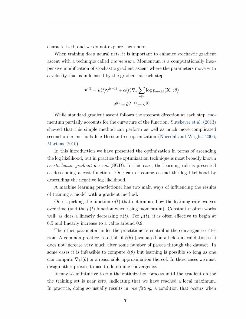
When training deep neural nets, it is important to enhance stochastic gradient
ascent with a technique called momentum. Momentum is a computationally inex-
pensive modification of stochastic gradient ascent where the parameters move with
a velocity that is influenced by the gradient at each step:
v(t) = µ(t)v(t�1) + ↵(t)r✓
X
i2S
log pmodel
(Xi:
; ✓)
✓(t) = ✓(t�1) + v(t)
While standard gradient ascent follows the steepest direction at each step, mo-
mentum partially accounts for the curvature of the function. Sutskever et al. (2013)
showed that this simple method can perform as well as much more complicated
second order methods like Hessian-free optimization (Nocedal and Wright, 2006;
Martens, 2010).
In this introduction we have presented the optimization in terms of ascending
the log likelihood, but in practice the optimization technique is most broadly known
as stochastic gradient descent (SGD). In this case, the learning rule is presented
as descending a cost function. One can of course ascend the log likelihood by
descending the negative log likelihood.
A machine learning practictioner has two main ways of influencing the results
of training a model with a gradient method.
One is picking the function ↵(t) that determines how the learning rate evolves
over time (and the µ(t) function when using momentum). Constant ↵ often works
well, as does a linearly decreasing ↵(t). For µ(t), it is often e↵ective to begin at
0.5 and linearly increase to a value around 0.9.
The other parameter under the practitioner’s control is the convergence crite-
rion. A common practice is to halt if `(✓) (evaluated on a held-out validation set)
does not increase very much after some number of passes through the dataset. In
some cases it is infeasible to compute `(✓) but learning is possible so long as one
can compute r✓
`(✓) or a reasonable approximation thereof. In these cases we must
design other proxies to use to determine convergence.
It may seem intuitive to run the optimization process until the gradient on the
the training set is near zero, indicating that we have reached a local maximum.
In practice, doing so usually results in overfitting, a condition that occurs when
7
the model memorizes spurious patterns in the training set and as a result obtains
much worse accuracy on the test set. Generally, in machine learning applications,
we care about performance on the test set, which we can estimate by monitoring
performance on a held out validation set. The best criteria for deep learning usually
are based on validation set performance. The main goal of such criteria is to
prevent overfitting, not to make sure that a maximum has been reached. A common
approach is to store the parameters that have attained the best accuracy on the
validation set, and stop training when no new best parameters have been found
within some fixed number of update steps. At the end of training, we use the best
stored parameters, not the last parameters visited by SGD.
Many other sophisticated optimization algorithms exist, but they have not
proven as e↵ective for deep learning as stochastic gradient and momentum have.
1.2 Supervised learning
Supervised learning is the class of learning problems where the desired output of
the model on some training set is known in advance and supplied by a supervisor.
One example of this is the aforementioned classification problem, where the learned
model is a function f(x) that maps examples x to category IDs. Another common
supervised learning problem is regression. In the context of regression, the training
set consists of a design matrix X and a vector of real-valued targets y 2 Rm (or a
matrix of outputs in the case of multiple output targets for each example). In this
work, we do not study regression.
It is possible to solve the classification problem using maximum likelihood es-
timation and stochastic gradient ascent. One simply fits a model p(y | x; ✓) or
p(x, y; ✓) to the training set, and returns f(x) = argmaxy
p(y | x).
The maximum likelihood approach is the one most commonly employed in deep
learning. We describe deep supervised learning in more detail in chapter 3.
Among shallow learning models, one of the best known supervised learning
approaches is the support vector machine.
8
1.2.1 Support vector machines and statistical learning the-
ory
The support vector machine (SVM) is a widely used model and associated learn-
ing algorithm for supervised learning. SVMs may be used to solve both regression
(Drucker et al., 1996) and classification (Cortes and Vapnik, 1995) problems. We
found classification SVMs useful for some of the work described in this thesis.
When solving the classification problem, an SVM discriminates between two
classes. In order to solve a k-class classification problem, one may train k di↵erent
SVMs. SVM i learns to discriminate class i from the other k � 1 classes. This is
called one-against-all classification (bo Duan and Keerthi, 2005). Other methods
of solving multi-class problems exist, but this is the one we use in the current work.
When training a basic two-class SVM it is conventional to regard labels yi
as
drawn from {�1, 1}. This makes some of the algebraic expressions that follow more
compact. Examples belonging to class 1 are referred to as positive examples while
examples belong to class -1 are known as negative examples.
The SVM works by finding a hyperplane that separates the positive examples
from the negative examples as well as possible (di↵erent kinds of SVMs have dif-
ferent ways of quantifying “as well as possible,” and the simplest form of SVM
is only applicable to data that can be separated perfectly). This hyperplane
is parameterized by a vector w and a scalar b. The classification function is
f(x) = sign(w>x+b). In order to obtain good generalization, none of the examples
should lie very close to the hyperplane. If a training example lies close to the hy-
perplane, a similar test example might cross the hyperplane and receive a di↵erent
label. To this end, SVM training algorithms try to ensure that y(w>x+ b) � 1 for
all training examples x.
SVMs are commonly used with the kernel trick. The kernel trick replaces dot
products x>z with evaluations of a kernel function K(x, z) = �(x)>�(z). All
operations that the SVM and its training algorithm perform on the input can be
written in terms of dot products x>z. By replacing these dot products with K(x, z),
one can train the SVM in �-mapped space rather than the original space. Clever
choices of K allow the use of high-dimensional, even infinite-dimensional, �. In the
case of non-linear �, the SVM will have a non-linear decision boundary rather than
a separating hyperplane in the original data space. Its decision function will still
9
be a hyperplane in �-mapped space. While the kernel trick is popular, it has many
disadvantages, including requiring the training algorithm to be adapted in ways
that reduce its ability to scale to very large numbers of training examples. Because
of these di�culties, we do not use the kernel trick in this work. The deep learning
methods employed in this thesis can be considered as analogous to learning the
kernel.
Various methods of training SVMs exist. We found that a variant called the L2-
SVM (Keerthi et al., 2005) is easy to train and obtains the best generalization on the
tasks we consider here. The L2-SVM is controlled by a regularization parameter C.
C must be positive and it determines the cost of misclassifying a training example.
Larger values of C mean that the SVM will learn to have higher accuracy on the
training set. Too large of a value of C can however result in overfitting.
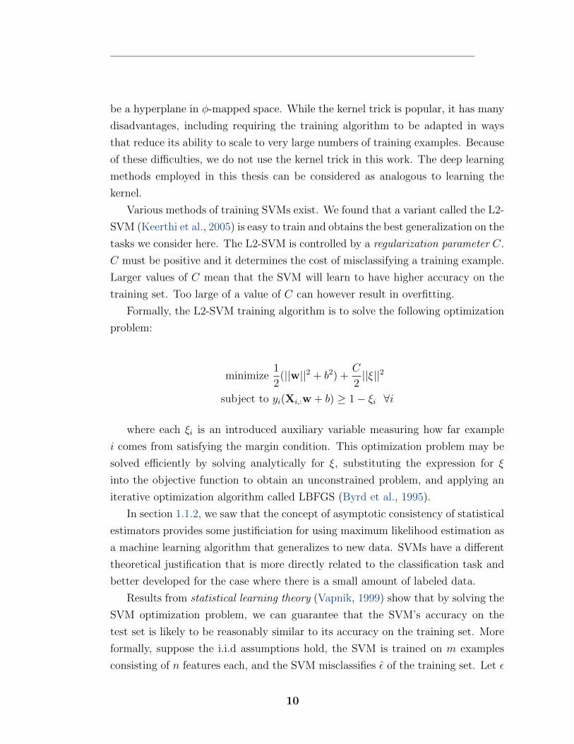
Formally, the L2-SVM training algorithm is to solve the following optimization
problem:
minimize1
2(||w||2 + b2) +
C
2||⇠||2
subject to yi
(Xi,:
w + b) � 1 � ⇠i
8i
where each ⇠i
is an introduced auxiliary variable measuring how far example
i comes from satisfying the margin condition. This optimization problem may be
solved e�ciently by solving analytically for ⇠, substituting the expression for ⇠
into the objective function to obtain an unconstrained problem, and applying an
iterative optimization algorithm called LBFGS (Byrd et al., 1995).
In section 1.1.2, we saw that the concept of asymptotic consistency of statistical
estimators provides some justificiation for using maximum likelihood estimation as
a machine learning algorithm that generalizes to new data. SVMs have a di↵erent
theoretical justification that is more directly related to the classification task and
better developed for the case where there is a small amount of labeled data.
Results from statistical learning theory (Vapnik, 1999) show that by solving the
SVM optimization problem, we can guarantee that the SVM’s accuracy on the
test set is likely to be reasonably similar to its accuracy on the training set. More
formally, suppose the i.i.d assumptions hold, the SVM is trained on m examples
consisting of n features each, and the SVM misclassifies ✏ of the training set. Let ✏
10
represent the proportion of examples drawn from pdata
that the SVM misclassifies
(i.e., its error rate on an infinitely large test set). For any � 2 (0, 1) we can
guarantee (Vapnik and Chervonenkis, 1971)
with probability 1 � �, ✏ ✏ +
s(n + 1) log( 2m
n+1
+ 1) � log( �
4
)
m
This is a conservative bound; it applies to any pdata
and any classifier based
on a separating hyperplane. Real-world distributions usually result in much better
test set performance. It is also possible to obtain tighter bounds that are specific
to SVMs.
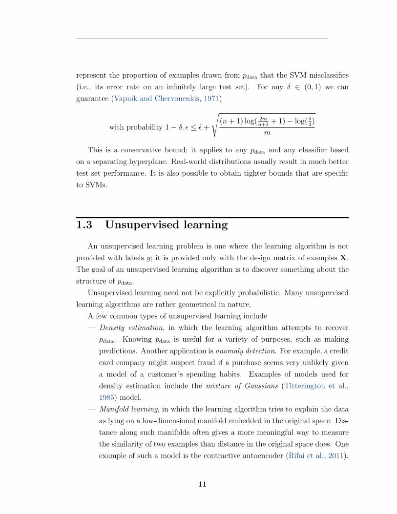
1.3 Unsupervised learning
An unsupervised learning problem is one where the learning algorithm is not
provided with labels y; it is provided only with the design matrix of examples X.
The goal of an unsupervised learning algorithm is to discover something about the
structure of pdata
.
Unsupervised learning need not be explicitly probabilistic. Many unsupervised
learning algorithms are rather geometrical in nature.
A few common types of unsupervised learning include
— Density estimation, in which the learning algorithm attempts to recover
pdata
. Knowing pdata
is useful for a variety of purposes, such as making
predictions. Another application is anomaly detection. For example, a credit
card company might suspect fraud if a purchase seems very unlikely given
a model of a customer’s spending habits. Examples of models used for
density estimation include the mixture of Gaussians (Titterington et al.,
1985) model.
— Manifold learning, in which the learning algorithm tries to explain the data
as lying on a low-dimensional manifold embedded in the original space. Dis-
tance along such manifolds often gives a more meaningful way to measure
the similarity of two examples than distance in the original space does. One
example of such a model is the contractive autoencoder (Rifai et al., 2011).
11
— Clustering, in which the learning algorithm attempts to discover a set of
categories that the data can be divided into neatly. For example, an online
store might cluster its customers based on their purchasing habits. When
a new customer buys one item, the store can see which cluster of previous
customers tends to buy that item the most, and recommend other items
bought by customers in that cluster. Examples of clustering algorithms
include k-means (Steinhaus, 1957) and mean-shift (Fukunaga and Hostetler,
1975) clustering.
These are not necessarily mutually exclusive categories (density estimation is
commonly but not always used to achieve all of the others). Nor are all of their goals
clearly defined (a dataset of carrots, oranges, radishes, and apples could equally well
be divided into two clusters consisting of fruit and vegetables or into two clusters
consisting of orange objects and red objects).
As an example, the mixture of Gaussians model supposes that the data can
be divided into k di↵erent categories. A latent variable h 2 {1, . . . , k} whose dis-
tribution is governed by a parameter c identifies which category a given example
belongs to. The distribution over members of category i is given by a multivari-
ate Gaussian distribution with mean µ(i) and covariance matrix ⌃(i). Often ⌃ is
restricted to be a diagonal matrix for computational and statistical reasons. The
complete generative model is:
p(h = i) = ci
p(x | h) = N (x | µ(h),⌃(h)).
This model can be fit with straightforward maximum likelihood estimation tech-
niques. Fitting the model accomplishes both a density estimation task and a clus-
tering task– an example x belongs to the cluster argmaxh
p(h | x).
1.4 Feature learning
Feature learning (also known as representation learning) is an important strat-
egy in machine learning. Many learning problems become “easier” if the inputs x
are transformed to a new set of inputs �(x). Properly designed feature mappings
12
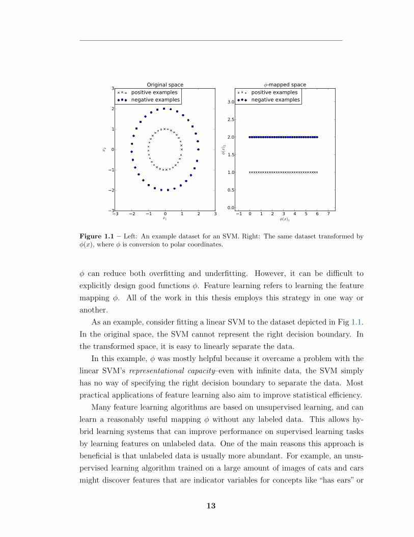
Figure 1.1 – Left: An example dataset for an SVM. Right: The same dataset transformed by�(x), where � is conversion to polar coordinates.
� can reduce both overfitting and underfitting. However, it can be di�cult to
explicitly design good functions �. Feature learning refers to learning the feature
mapping �. All of the work in this thesis employs this strategy in one way or
another.
As an example, consider fitting a linear SVM to the dataset depicted in Fig 1.1.
In the original space, the SVM cannot represent the right decision boundary. In
the transformed space, it is easy to linearly separate the data.
In this example, � was mostly helpful because it overcame a problem with the
linear SVM’s representational capacity–even with infinite data, the SVM simply
has no way of specifying the right decision boundary to separate the data. Most
practical applications of feature learning also aim to improve statistical e�ciency.
Many feature learning algorithms are based on unsupervised learning, and can
learn a reasonably useful mapping � without any labeled data. This allows hy-
brid learning systems that can improve performance on supervised learning tasks
by learning features on unlabeled data. One of the main reasons this approach is
beneficial is that unlabeled data is usually more abundant. For example, an unsu-
pervised learning algorithm trained on a large amount of images of cats and cars
might discover features that are indicator variables for concepts like “has ears” or
13
“has wheels.” A classifier trained with these high-level input features then needs
few labeled examples in order to generalize well.
Even when all of the available examples are labeled, training the features to
model the input can provide some regularization.
Unsupervised feature learning is also useful because it allows the model to be
split into pieces and trained one component at a time, even if each individual
component cannot be meaningfully associated with an output target. For example,
if we divide a 32 ⇥ 32 pixel image of a cat into a collection of small 6 ⇥ 6 pixel
image patches, many of these patches do not contain any portion of the cat at all
and those that do contain some portion of the cat probably do not contain enough
information to identify it. We therefore cannot associate each image patch with a
label, so supervised learning cannot make progress with the input divided up in this
way. Unsupervised learning can still learn good descriptions of each image patch,
allowing us to learn thousands of features per image patch. When extracted at all
locations in the image, this corresponds to millions of features per image. Learning
these millions of features on a per-patch basis greatly reduces the computational
cost of training such a system. This patch-based learning approach has been used in
several practical applications (Lee et al., 2009; Coates et al., 2011) and is exploited
in this thesis.
A closely related idea to feature learning is deep learning (Bengio, 2009). In deep
learning, the feature extractor � is formed by composing several simpler mappings:
�(x) = �(L)(�(L�1)(. . . �(1)(x)))
where L is the total number of mappings. Each mapping �(i) is known as a layer.
The composite feature extractor � is considered “deep” because the computational
graph describing it has several of these layers. Each layer of a deep learning system
can be thought of as being analogous to a line of code in a program–each layer
references the results of earlier layers, and complicated tasks can be accomplished
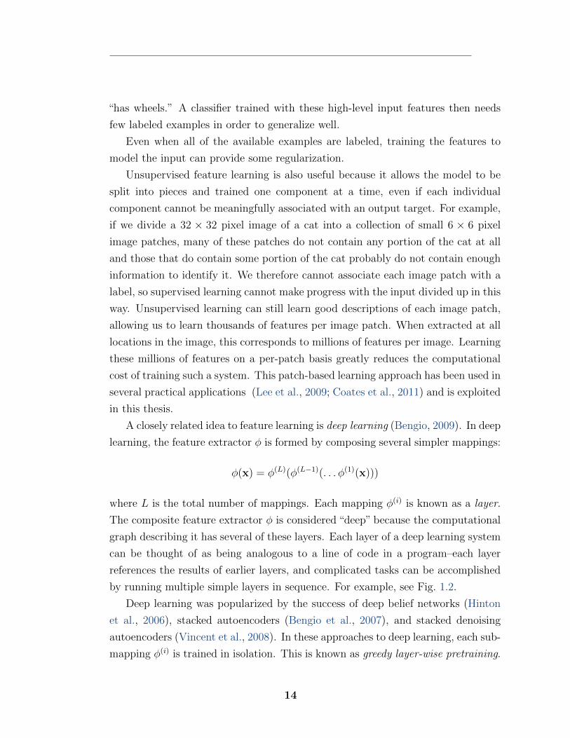
by running multiple simple layers in sequence. For example, see Fig. 1.2.
Deep learning was popularized by the success of deep belief networks (Hinton
et al., 2006), stacked autoencoders (Bengio et al., 2007), and stacked denoising
autoencoders (Vincent et al., 2008). In these approaches to deep learning, each sub-
mapping �(i) is trained in isolation. This is known as greedy layer-wise pretraining.
14
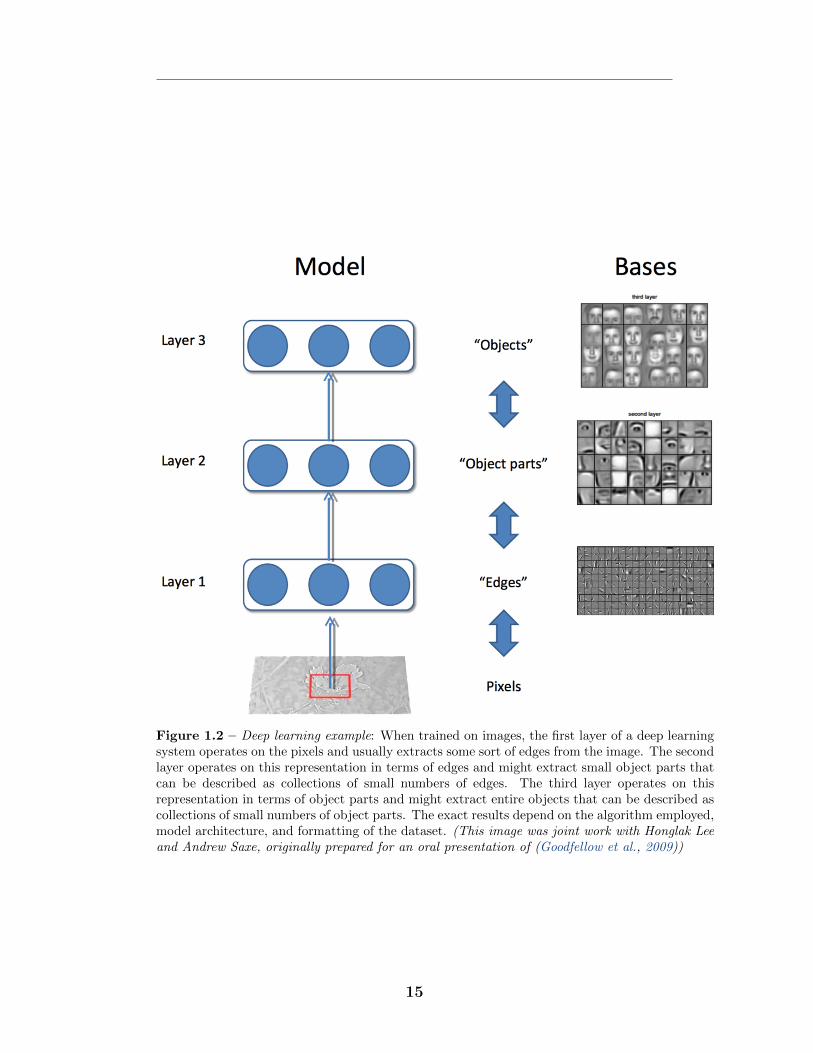
Figure 1.2 – Deep learning example: When trained on images, the first layer of a deep learningsystem operates on the pixels and usually extracts some sort of edges from the image. The secondlayer operates on this representation in terms of edges and might extract small object parts thatcan be described as collections of small numbers of edges. The third layer operates on thisrepresentation in terms of object parts and might extract entire objects that can be described ascollections of small numbers of object parts. The exact results depend on the algorithm employed,model architecture, and formatting of the dataset. (This image was joint work with Honglak Leeand Andrew Saxe, originally prepared for an oral presentation of (Goodfellow et al., 2009))
15
This pretraining is usually followed by joint fine-tuning of the entire system.
Since this style of deep learning system is formed by composing shallow learn-
ers, a popular form of deep learning research is devising new shallow learners.
Some examples of recent work in developing shallow learners for feature learn-
ing includes work with sparse coding (Raina et al., 2007), restricted Boltzmann
machines (RBMs) (Hinton et al., 2006; Courville et al., 2011a), the aforemen-
tioned autoencoder-based methods, and hybrids of autoencoders and sparse cod-
ing (Kavukcuoglu et al., 2010a). The spike-and-slab sparse coding work we intro-
duce in chapter 5 can be seen as a continuation of this line of research.
Other approaches to deep learning involve training the entire deep learning
system simultaneously. This is the approach we use in the remainder of this thesis.
16
2 Structured Probabilistic
Models
Chapter 1 presented some of the basic ideas of probabilistic modeling with
maximum likelihood estimation. This chapter explores these ideas in greater depth,
applying maximum likelihood estimation to more complicated models that require
us to introduce approximations.
Sections 2.1 and 2.2 describe two ways of representing structure in a probabilistic
model. Viewing probabilistic models as containing simplifying structure is a crucial
cognitive tool that motivates design choices throughout the rest of this thesis.
Section 2.3 explains a basic design choice about how to represent complicated
interactions between multiple units.
Section 2.4 explains how to train models for which the likelihood cannot be
computed using sampling-based approximations to the gradient of the log likeli-
hood. Other approximate methods of training are possible for these models but
the strategies detailed in this section are the ones that are used in this thesis.
Section 2.5, demonstrates how models with an intractable posterior distribution
over their latent variables can be trained using variational approximations. Again,
other approximations are possible, so the presentation here focuses on the methods
actually used in the present work.
Finally, I’ll discuss combining both forms of approximation in section 2.6.
2.1 Directed models
In general, a probability distribution over a vector-valued variable x repre-
sents probabilistic interactions between all of the variables. Suppose that x 2{1, . . . , k}n. To parameterize a fully general P (x) on discrete data like this is re-
quires a table containing kn � 1 entries! (one entry for all but one of the members
17
of the outcome space, with the probability of the last entry determined by the
constraint that a probability distribution sum to 1)
Fortunately, most probability distributions we actually work with in practice do
not involve all possible interactions between all possible variables. Many variables
interact with each other only indirectly. This allows us to greatly simplify our
representation of the distribution.
Probabilistic models that exploit this idea are called structured probabilistic
models, because they represent the variables as belonging to a structure that re-
stricts their ability to interact directly. Structure enables a model to do its job with
fewer parameters, thus reducing the computational cost of storing it and increas-
ing its statistical e�ciency. It also reduces the computational cost of performing
operations like computing marginal or conditional distributions over subsets of the
variables (Koller and Friedman, 2009).
A common form of structured probabilistic model is the Bayesian network
(Pearl, 1985). A Bayesian network is defined by a directed acyclic graph G whose
vertices are the random variables in the model, and a set of local conditional prob-
ability distributions p(xi
| PaG(xi
)) where PaG(xi
) returns the parents of xi
in G.
The probability distribution over x is given by
p(x) = ⇧i
p(xi
| PaG(xi
)).
So long as each variable has few parents in the graph, the distribution can be
represented with very few parameters. Simple restrictions on the graph structure
can also guarantee that operations like computing marginal or conditional distri-
butions over subsets of variables are e�cient.
2.2 Undirected models
Some interactions between variables may not be well-captured by local con-
ditional probability distributions. For example, when modeling the pixels in an
image, there is no clear reason for one pixel to be a parent of the other; their
interactions are basically symmetrical.
18
A Markov network (Kindermann, 1980) is a structured graphical model defined
on an undirected graph G. For each clique C in the graph, a factor �(C) measures the
a�nity of the variables in that clique for being in each of their possible states. The
factors are constrained to be non-negative. Together they define an unnormalized
probability distribution
p(x) = ⇧C2G�(C).
The unnormalized probability distribution is e�cient to work with so long as
all the cliques are small.
Obtaining the normalized probability distribution may be costly. To do so,
one must compute the partition function Z (though Z is conventionally written
without arguments, it is in fact a function of whatever parameters govern each of
the � functions). Since
Z =
Z
x
p(x)dx
it may be intractable to compute for high-dimensional x, depending on the
structure of G and the functional form of the �s.
Many interesting theoretical results about undirected models depend on the
assumption that 8x, p(x) > 0. A convenient way to enforce this to use an energy-
based model (EBM) where
p(x) = exp(�E(x))
and E(x) is known as the energy function. This can still be interpreted as a
standard Markov network; the exponentation makes each term in the energy func-
tion correspond to a factor for a di↵erent clique. The � sign isn’t strictly necessary
from a computational point of view (and some machine learning researchers have
tried to do without it, e.g. (Smolensky, 1986)). It is a commonly used conven-
tion inherited from statistical phyiscs, along with the terms “energy function” and
“partition function.”
Some results in this chapter are presented in terms of energy-based models. For
these results, the theory doesn’t hold if p(x) = 0 for some x. Note that a directed
graphical model may be encoded as an energy-based model so long as this condition
is respected.
19
2.2.1 Sampling
Drawing a sample x from the probability distribution p(x) defined by a struc-
tured model is an important operation. We briefly describe how to sample from
directed models and EBMs here. For more detail, see (Koller and Friedman, 2009).
Sampling from a directed model is straightforward, assuming that one can sam-
ple from each of the conditional probability distributions. The procedure used in
this case is called ancestral sampling. One simply draws samples of each of the
variables in the network in an order that respects the network topology, i.e., before
sampling a variable xi
from P (xi
| Paxi), sample each of the members of Pa
xi . This
defines an e�cient means of sampling all variables with a single pass through the
network.
Sampling from an EBM is not straightforward. Suppose we have an EBM
defining a distribution p(a, b). In order to sample a, we must draw it from p(a | b),
and in order to sample b, we must draw it from p(b | a). This “chicken and
egg” problem means we can no longer use ancestral sampling. Since G is no longer
directed and acyclical, we don’t have a way of ordering the variables such that every
variable can be sampled given only variables that come earlier in the ordering.
It turns out that we can sample from an EBM, but we can not generally do
so with a single pass through the network. Instead we need to sample using a
Markov chain. A Markov chain is defined by a state x and a transition distribution
T (x0 | x). Running the Markov chain means repeatedly updating the state x to a
value x0 sampled from T (x0 | x).
Under certain distributions, a Markov chain is eventually guaranteed to draw
x from an equilibrium distribution ⇡(x0), defined by the condition
8x0, ⇡(x0) =X
x
T (x0 | x)⇡(x).
This condition guarantees that repeated applications of the transition sampling
procedure don’t change the distribution over the state of the Markov chain. Run-
ning the Markov chain until it reaches its equilibrium distribution is called“burning
in” the Markov chain.
Unfortunately, there is no theory to predict how many steps the Markov chain
must run before reaching its equilibrium distribution, nor any way to tell for sure
that this event has happened. Also, even though successive samples come from the
20
same distribution, they are highly correlated with each other, so to obtain multiple
independent samples one should run the Markov chain for several steps between
collecting each sample. Markov chains tend to get stuck in a single mode of ⇡(x)
for several steps. The speed with which a Markov chain moves from mode to mode
is called its mixing rate. Since burning in a Markov chain and getting it to mix
well may take several sampling steps, sampling correctly from an EBM is still a
somewhat costly procedure.
Of course, all of this depends on ensuring ⇡(x) = p(x) . Fortunately, this is easy
so long as p(x) is defined by an EBM. The simplest method is to use Gibbs sampling,
in which sampling from T (x0 | x) is accomplished by selecting one variable xi
and
sampling it from p conditioned on its neighbors in G. It is also possible to sample
several variables at the same time so long as they are conditionally independent
given all of their neighbors.
2.3 Latent variables
Most of this thesis concerns models that have two types of variables: observed
or “visible” variables v and latent or “hidden” variables h. v corresponds to the
variables actually provided in the design matrix X during training. h consists of
variables that are introduced to the model in order to help it explain the structure
in v. Generally the exact semantics of h depend on the model parameters and are
created by the learning algorithm. The motivation for this is twofold.
2.3.1 Latent variables versus structure learning
Often the di↵erent elements of v are highly dependent on each other. A good
model of v which did not contain any latent variables would need to have very
large numbers of parents per node in a Bayesian network or very large cliques in a
Markov network. Just representing these higher order interactions is costly–both
in a computational sense, because the number of parameters that must be stored in
memory scales exponentially with the number of members in a clique, but also in a
statistical sense, because this exponential number of parameters requires a wealth
of data to estimate accurately.
21
There is also the problem of learning which variables need to be in such large
cliques. An entire field of machine learning called structure learning is devoted to
this problem . Most structure learning techniques involve fitting a model with a
specific structure to the data, assigning it some score that rewards high training
set accuracy and penalizes model complexity, then greedily adding or subtracting
an edge from the graph in a way that is expected to increase the score. See (Koller
and Friedman, 2009) for details of several approaches.
Using latent variables mostly avoids the problem of learning structure. A fixed
structure over visible and hidden variables can use direct interactions between
visible and hidden units to impose indirect interactions between visible units. Using
simple parameter learning techniques we can learn a model with a fixed structure
that imputes the right structure on the marginal p(v). Of course, one still has the
problem of determining the amount of latent variables and their connectivity, but it
is usually not as important to determine the absolutely optimal model architecture
when using latent variables as when using structure learning on fully observed
models. Usually, in the context of deep learning and latent variable models, the
architecture is controlled by a small number of hyperparameters, which are searched
relatively coarsely.
2.3.2 Latent variables for feature learning
Another advantage of using latent variables is that they often develop useful
semantics. As discussed in section 1.3, the mixture of Gaussians model learns a
latent variable that corresponds to which category of examples the input was drawn
from. Other more sophisticated models with more latent variables can create even
richer descriptions of the input. Most of the approaches mentioned in section 1.4
accomplish feature learning by learning latent variables. Often, given some model
of v and h, it turns out that E[h | v] or argmaxh
p(h,v) is a good feature mapping
for v.
22
2.4 Stochastic approximations to maximum
likelihood
Consider an energy-based model p(v,h) = 1
Z
exp(�E(v,h)).
Suppose that the partition function Z cannot be computed. This model may
still be useful. As explained in section 2.2.1, one can still draw samples from this
model, perhaps even e�ciently. One might also be able to compute the ratio of
the probability of two events, p(v,h)/p(v0,h0), or the posterior p(h | v), which as
shown in 2.3 could be useful as a set of features to describe v.
Given that such a model is useful, learning one is a desirable capability. How-
ever, our primary method of learning models is maximum likelihood estimation.
As seen in section 1.1.3, this involves computing
r✓
log p(v).
Unfortunately, if we expand the definition of p(v), we see that this expression
contains Z:
r✓
log p(v) � r✓
log Z.
Since Z is intractable, there doesn’t seem to be much hope of computing
r✓
log Z.
Fortunately, so long as Leibniz’s rule applies, a sampling trick can approximate
the gradient:
23
@
@✓i
log Z
=@
@✓i
log
Z
v
Z
h
p(v,h)dhdv
=@
@✓i
Rv
Rh
p(v,h)dhdvRv
Rh
p(v,h)dhdv
=1
Z
Z
v
Z
h
@
@✓i
exp(�E(v,h))dhdv
= � 1
Z
Z
v
Z
h
exp(�E(v,h))@
@✓i
E(v,h)dhdv
= �Ev,h
[@
@✓i
E(v,h)]
The expectation can be approximated by drawing samples of v and h, but this
of course raises the question of how to set up the Markov chain in a way that yields
a good approximation and is e�cient.
The naive approach is to initialize a new Markov chain and run it to its equilib-
rium distribution on every step of stochastic gradient ascent. Unfortunately, that
is too expensive.
One solution to this problem is contrastive divergence (CD-k) (Hinton, 2002).
This approach makes use of several Markov chains in parallel, one per example
in the minibatch. At each learning step, each Markov chain is initialized with
the corresponding data example and run for k steps. Typically k = 1. Clearly this
approach only explores parts of space that are near the data points. This procedure
generally results in the model’s distribution having about the right shape near the
data points, but the model may inadvertently learn to represent other modes far
from the data.
Another approach is known alternatively as stochastic maximum likelihood (SML)
(Younes, 1998) or persistent contrastive divergence (PCD) (Tieleman, 2008). This
approach also makes use of parallel Markov chains but each is initialized only once,
at the start of training. The state of each chain is sampled once per gradient
ascent step. This approach depends on the assumption that the learning rate is
small enough that the Markov chains will remain at their equilibrium distribution
24
h1
h2
h3
v1
v2
v3
h4
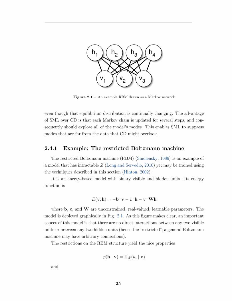
Figure 2.1 – An example RBM drawn as a Markov network
even though that equilibrium distribution is continually changing. The advantage
of SML over CD is that each Markov chain is updated for several steps, and con-
sequently should explore all of the model’s modes. This enables SML to suppress
modes that are far from the data that CD might overlook.
2.4.1 Example: The restricted Boltzmann machine
The restricted Boltzmann machine (RBM) (Smolensky, 1986) is an example of
a model that has intractable Z (Long and Servedio, 2010) yet may be trained using
the techniques described in this section (Hinton, 2002).
It is an energy-based model with binary visible and hidden units. Its energy
function is
E(v,h) = �b>v � c>h � v>Wh
where b, c, and W are unconstrained, real-valued, learnable parameters. The
model is depicted graphically in Fig. 2.1. As this figure makes clear, an important
aspect of this model is that there are no direct interactions between any two visible
units or between any two hidden units (hence the “restricted”; a general Boltzmann
machine may have arbitrary connections).
The restrictions on the RBM structure yield the nice properties
p(h | v) = ⇧i
p(hi
| v)
and
25
p(v | h) = ⇧i
p(vi
| h).
The individual conditionals are simple to compute as well, for example
p(hi
= 1 | v) = ��v>W
i
+ bi
�
where � is the logistic sigmoid function.
Together these properties allow for e�cient block Gibbs sampling, alternating
between sampling all of h simultaneously and sampling all of v simultaneously.
Since the energy function itself is just a linear function of the parameters, it is
easy to take the needed derivatives. For example,
@
@Wij
E(v,h) = �vi
hj
.
These two properties–e�cient Gibbs sampling and e�cient derivatives– make
it possible to train the RBM with stochastic approximations to r✓
log Z.
2.5 Variational approximations
Another common di�culty in probabilistic modeling is that for many models
the posterior distribution p(h | v) is infeasible to compute or even represent. Alter-
nately, it may be infeasible to take expectations with respect to this distribution.
This poses problems for our goal outlined in section 2.3.2 of using E[h | v] as
features. It also usually means that maximum likelihood estimation is infeasible.
As shown in (Neal and Hinton, 1999), maximizing p(v) is equivalent to maximizing
Eh⇠P (h|v)
log P (v,h).
Fortunately, variational approximations provide a solution to both of these dif-
ficulties.
26
2.5.1 Variational learning
For any distribution Q(h), the log likelihood may be decomposed (Neal and
Hinton, 1999) into two terms.
log p(v) = DKL
(Q(h)kp(h | v)) + L(v, Q).
Here, DKL
is the Kullback-Leibler (KL) divergence (Kullback and Leibler, 1951)
and L is the negative variational free energy. The KL divergence is guaranteed to
be non-negative, so this decomposition proves
log p(v) � L(v, Q).
L(v, Q) is thus a lower bound on the log likelihood. The KL divergence measures
the di↵erence between two distributions, and goes to 0 when the two distributions
are the same. Thus this lower bound is tight when Q(h) = P (h | v). Consequently,
one can maximize L(v, Q) as a proxy for log p(v). Note that this maximization
will involve modifying both the distribution Q (to make the lower bound tighter)
and the parameters controlling p (to optimize the model using the bound).
In order to maximize L, let’s examine its functional form:
L(v, Q) = Eh⇠Q
[log P (v,h)] + HQ
(h)
where HQ
(h) is the Shannon entropy (Cover, 2006) of h under Q.
Since computing L(v, Q) involves taking an expectation with respect to Q, it is
necessary to restrict Q in order to make the expectation tractable. A particularly
elegant way to restrict Q is to require it to take the form of a graphical model with
a specific graph structure G (Saul and Jordan, 1996). A common approach is to
use the mean field approximation
Q(h) = ⇧i
Q(hi
)
which corresponds to a G with no edges. So long as inference in Q remains tractable,
one can obtain better approximations by using a more complicated G. This ap-
proach is known as structured variational approximation.
27
2.5.2 Variational inference
A common operation is to compute the Q that minimizes DKL
(Q(h)kP (h | v)).
This is necessary for extracting features E[h | v]. It is also a common inner-loop to
variational learning algorithms which alternate between optimizing L(v, Q) with
respect to Q and optimizing it with respect to the model parameters.
This operation is called variational inference (Koller and Friedman, 2009) be-
cause in the general case it involves solving a calculus of variations problem. Calcu-
lus of variations is the study of optimizing functionals. A functional is a mapping
much like a function, except that a functional takes a function as its input. In
variational inference, the functional being minimized is the KL divergence. The
function being optimized is the distribution Q. Note that in the special case where
none of the h variables is continuous, Q is merely a vector and may be optimized
with traditional calculus techniques.
Usually variational inference involves using calculus of variations to find the
functional form of Q, followed by an iterative procedure to find the parameters of
Q. Consider the following example from (Bishop, 2006).
Suppose h 2 R2 and p(h | v) = N (h | µ, ��1) (for the purpose of simplicity, in
this example, the hidden units do not actually interact with the visible units).
Constrain Q with the mean field assumption Q(h) = Q(h1
)Q(h2
). Using calcu-
lus of variations one may then show
Q(hi
) = N (hi
| hi
, 1/�i,i
).
In other words, the fact that p(h | v) is jointly Gaussian implies that the
correct Q is also Gaussian. We never assumed that Q was Gaussian, only that it
was factorial. The Gaussian nature of Q had to be derived via calculus of variations.
There is still an unknown: the mean of Q, h. This is an example of a variational
parameter, a parameter controlling Q that cannot be found analytically. These
parameters must be obtained by an iterative optimization procedure. Gradient
descent would work, but is a slow and expensive procedure to use in the inner
loop of a learning algorithm. Typically it is faster to optimize these parameters by
iterating between fixed point equations.
28
2.6 Combining approximations: The deep
Boltzmann machine
This chapter has described the tools needed to fit a very broad class of proba-
bilistic models. Which tool to use depends on which aspects of the log-likelihood
are problematic.
For the simplest distributions p, the log likelihood is tractable, and the model
can be fit with a straightforward application of maximum likelihood estimation and
gradient ascent as described in chapter 1.
This chapter has shown to implement probabilistic models in two di↵erent di�-
cult cases. In the case where Z is intractable, one may still use maximum likelihood
estimation via the sampling approximation techniques described in section 2.4. In
the case where p(h | v) is intractable, one may still train the model using the
negative variational free energy rather than the likelihood, as described in 2.5.
It is also possible that both of these di�culties will arise. An example of this
occurs with the deep Boltzmann machine (Salakhutdinov and Hinton, 2009), which
is a sequence of RBMs chained together with undirected connections. The model
is depicted graphically in Fig. 2.2.
This model still has the same problem with computing the partition function
as the simpler RBM does. It has also discarded the restricted structure that made
P (h | v) easy to represent in the RBM. The typical way to train the DBM is
to minimize the variational free energy rather than maximize the likelihood. Of
course, the variational free energy still depends on the partition function, so it is
necessary to use sampling techniques to approximate its gradient.
We put all of these techniques to use in chapter 5.2.2 when we introduce our
own partially-directed deep Boltzmann machine.
29
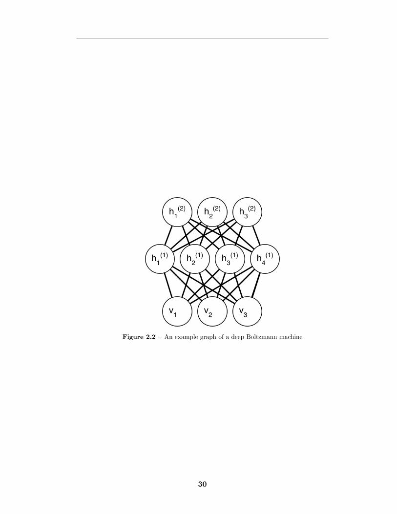
h1
(1) h2
(1) h3
(1)
v1
v2
v3
h1
(2) h2
(2) h3
(2)
h4
(1)
Figure 2.2 – An example graph of a deep Boltzmann machine
30
3 Supervised deep learning
The current version of deep learning models that is most widely used to solve
di�cult engineering problems for industrial scale applications is based on purely
supervised learning.
The standard deep learning model is the multilayer perceptron (MLP) , also
known as the feed-forward neural network (Rumelhart et al., 1986a). This consists
of a neural network that takes some input x and composes together transformations
defined by several layers to produce an output:
f(x) = fL
(fL�1
(. . . f1
(x)))
Each layer typically provides a matrix of learnable parameters W and a vector
of learnable parameters b defining an a�ne transformation of the input. If each
layer consisted only of an a�ne transformation, the entire function f would also
be a�ne, so each layer also includes some fixed non-linear activation function g:
fi
(v) = g(Wv + b).
Such models are motivated by a philosophy called connectionism (McClelland
et al., 1986). The idea behind connectionism is that an individual neuron in an
animal or a human being is not capable of doing anything interesting in isolation,
but populations of neurons acting together can achieve intelligent behavior. Sim-
ilarly, a single unit of a hidden layer in an MLP is useless, but any function can
be approximated with any desired non-zero amount of error by an MLP with su�-
ciently many hidden units (Cybenko, 1989; Stinchcombe and White, 1989; Hornik
et al., 1989). One can view humans and animals as a proof of concept illustrating
that di↵erent amounts of intelligent behavior are possible with the amount of com-
putational resources possessed by di↵erent species of animals. It may be possible
for us to design algorithms that use hardware even more e�ciently.
A special case of MLPs is the convolutional neural network (CNN). For a re-
31
cent review including a history of the development of this technique, see (Lecun,
Kavukcuoglu, and Farabet, Lecun et al.). This thesis is primarily concerned with
describing how the method works.
These networks restrict the structure of W and b for some of their layers.
Specifically, when the input to the layer can be seen as samples taken on a grid in
some space (for example, a rasterized image is a set of samples of brightness values
collected by a 2-D grid of sensors, an audio recording is a set of samples of amplitude
values collected on a 1-D grid throughout time, etc.), W may be restricted to
define a discrete convolution rather than a general matrix multiplication. This
makes Wx become equivariant to translations of the input. Because convolutions
use the same parameters at every location, this significantly reduces the number
of parameters that need to be stored and learned, improving both the model’s
memory requirements and statistical e�ciency. Typically, the kernel used for the
discrete convolution is small, meaning that the network is sparsely connected, which
further reduces the number of parameters, and reduces the runtime of inference and
backpropagation in the network.
Convolutional networks also typically include some kind of spatial pooling in
their activation functions g; this refers to taking summary statistics over small
spatial regions of the output in order to make the final output invariant to small
spatial translations of the input. CNNs have been very successful for commerical
image processing applications since the early 1990s. This commercial success con-
tinues today, with convolutional nets being used to perform a variety of computer
vision tasks (Krizhevsky et al., 2012; Zeiler and Fergus, 2013b; Szegedy et al., 2013;
Goodfellow et al., 2014).
MLPs and CNNs may be trained using stochastic gradient descent and mo-
mentum. The gradient, as defined by the chain rule of di↵erentiation, contains
very many terms. Fortunately, the di↵erent elements of the gradient contain many
common subexpressions. Using a dynamic programming 1approach, one can avoid
re-computing these subexpressions in order to compute the gradient e�ciently.
This idea is the basis of the backpropagation algorithm commonly used to compute
the gradient (Bryson et al., 1963; Werbos, 1974; Rumelhart et al., 1986b). Not all
1. “Dynamic programming” is an overloaded term and can refer to table-filling algorithms thatavoid repeatedly computing sommon subexpressions, or to iterating the Bellman equations. Herewe use the former sense of the term.
32
modern approaches necessarily use the backpropagation algorithm per se (di↵erent
choices of how to set up the dynamic programming process yield di↵erent speed-
memory tradeo↵s) but all do use symbolic di↵erentiation strategies that employ
the same basic dynamic programming technique.
Supervised deep learning has existed for decades and was even been used to
solve some commercial applications long before the recent resurgence in its pop-
ularity. However, some commercially interesting problems, such as general object
recognition, only recently became feasible to solve with this approach. This is for
three major reasons:
First, significantly larger labeled datasets are available now than were available
previously. This allows much larger models to be fit than was previously possible,
and reduces the need to design algorithms that avoid overfitting.
Second, until recently, the hardware and software infrastructure available did
not allow for training of su�ciently large networks. If we refer back to the bi-
ological inspiration for connectionism, and view biological intelligence as a proof
of concept giving some indication of what we can hope to achieve by simulating
di↵erent amounts of neurons, Fig. 3.1 shows that until recently our networks were
smaller than even the most primitive of biological nervous systems. As shown in
Fig. 3.2, machine learning models were able to compensate for this somewhat by
being nearly as densely connected as biological systems. However, we still lag ab-
solute scale of the human nervous system by many orders of magnitude. It is only
recently, with GPU-GPU implementations of machine learning algorithms (Chel-
lapilla et al., 2006), optimizing compilers for GP-GPU based on machine learning-
oriented domain-specific languages (Bergstra et al., 2010; Bastien et al., 2012) and
distributed (Dean et al., 2012) implementations of machine learning software that
we have started to approach the necessary scale. Maxout, presented in chapter 9,
can be seen as an attempt to increase the amount of feature detectors in the model
without requiring a proportional increase in connections between feature detectors.
Third, SGD often produces less than satisfactory results for the types of ac-
tivation functions g that were used until recently. The use of the rectified linear
activation function (Jarrett et al., 2009; Glorot et al., 2011)
g(z)i
= max{zi
, 0}
33
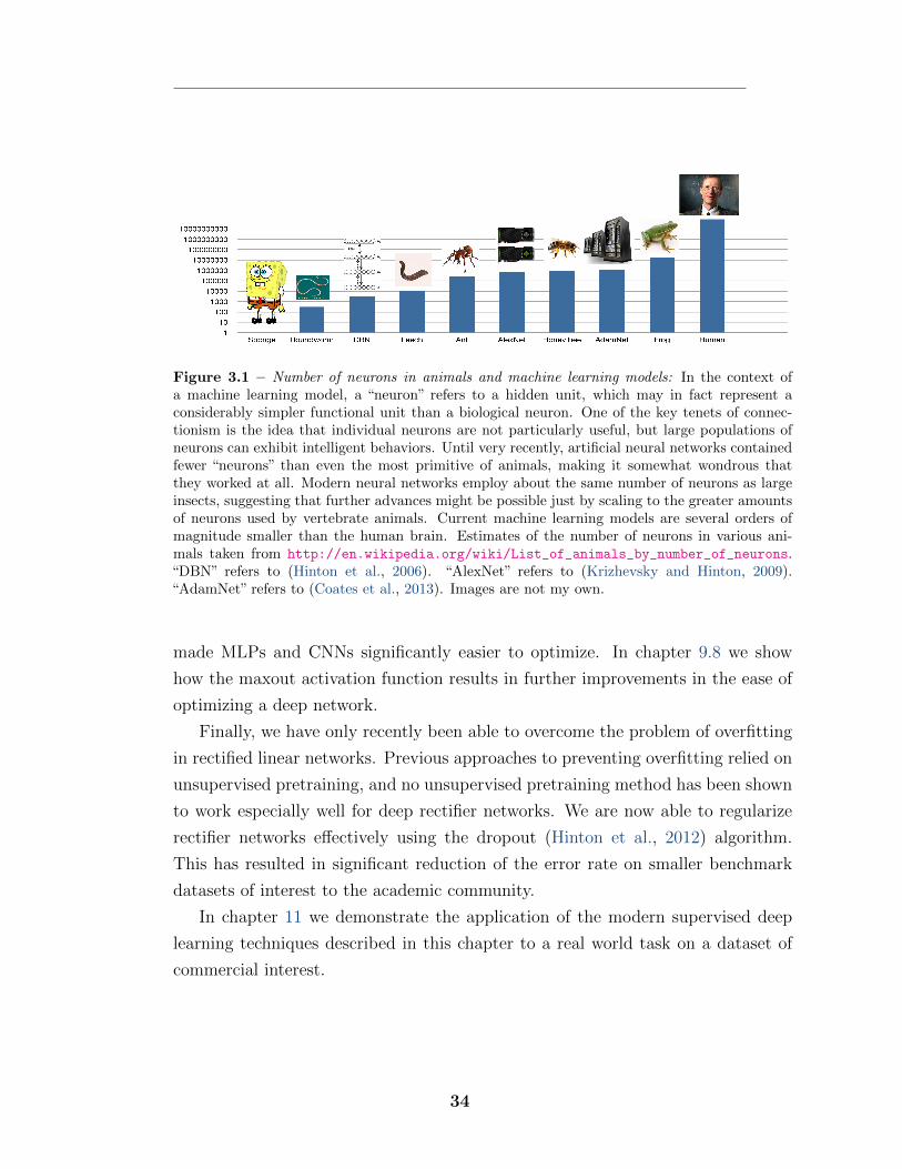
Figure 3.1 – Number of neurons in animals and machine learning models: In the context ofa machine learning model, a “neuron” refers to a hidden unit, which may in fact represent aconsiderably simpler functional unit than a biological neuron. One of the key tenets of connec-tionism is the idea that individual neurons are not particularly useful, but large populations ofneurons can exhibit intelligent behaviors. Until very recently, artificial neural networks containedfewer “neurons” than even the most primitive of animals, making it somewhat wondrous thatthey worked at all. Modern neural networks employ about the same number of neurons as largeinsects, suggesting that further advances might be possible just by scaling to the greater amountsof neurons used by vertebrate animals. Current machine learning models are several orders ofmagnitude smaller than the human brain. Estimates of the number of neurons in various ani-mals taken from http://en.wikipedia.org/wiki/List_of_animals_by_number_of_neurons.“DBN” refers to (Hinton et al., 2006). “AlexNet” refers to (Krizhevsky and Hinton, 2009).“AdamNet” refers to (Coates et al., 2013). Images are not my own.
made MLPs and CNNs significantly easier to optimize. In chapter 9.8 we show
how the maxout activation function results in further improvements in the ease of
optimizing a deep network.
Finally, we have only recently been able to overcome the problem of overfitting
in rectified linear networks. Previous approaches to preventing overfitting relied on
unsupervised pretraining, and no unsupervised pretraining method has been shown
to work especially well for deep rectifier networks. We are now able to regularize
rectifier networks e↵ectively using the dropout (Hinton et al., 2012) algorithm.
This has resulted in significant reduction of the error rate on smaller benchmark
datasets of interest to the academic community.
In chapter 11 we demonstrate the application of the modern supervised deep
learning techniques described in this chapter to a real world task on a dataset of
commercial interest.
34
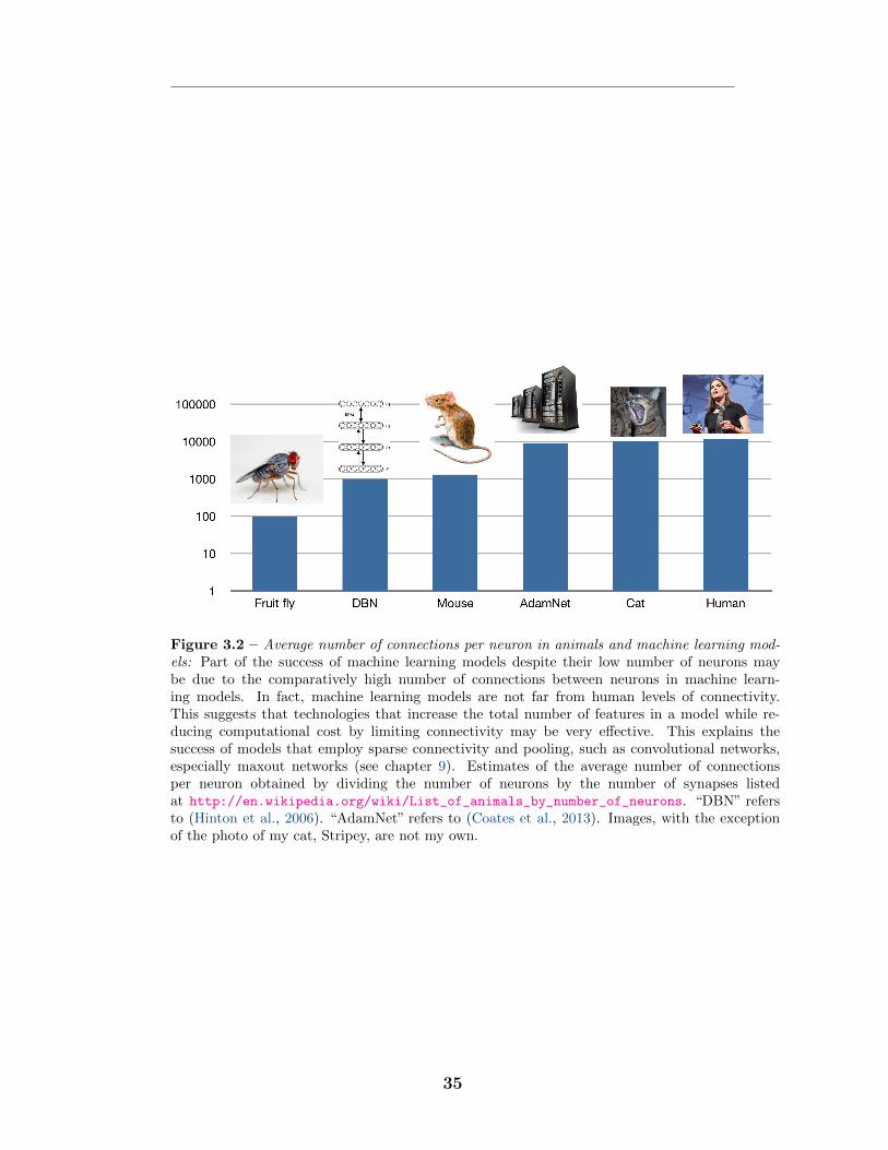
Figure 3.2 – Average number of connections per neuron in animals and machine learning mod-els: Part of the success of machine learning models despite their low number of neurons maybe due to the comparatively high number of connections between neurons in machine learn-ing models. In fact, machine learning models are not far from human levels of connectivity.This suggests that technologies that increase the total number of features in a model while re-ducing computational cost by limiting connectivity may be very e↵ective. This explains thesuccess of models that employ sparse connectivity and pooling, such as convolutional networks,especially maxout networks (see chapter 9). Estimates of the average number of connectionsper neuron obtained by dividing the number of neurons by the number of synapses listedat http://en.wikipedia.org/wiki/List_of_animals_by_number_of_neurons. “DBN” refersto (Hinton et al., 2006). “AdamNet” refers to (Coates et al., 2013). Images, with the exceptionof the photo of my cat, Stripey, are not my own.
35

4 Prologue to First Article
4.1 Article Details
Scaling up Spike-and-Slab Models for Unsupervised Feature Learn-
ing. Ian J. Goodfellow, Aaron Courville, and Yoshua Bengio. IEEE Transactions
on Pattern Analysis and Machine Intelligence 35 (8), 1902-1914.
Personal Contribution. The idea that a structured variational inference in a
sparse coding model could provide an e↵ective means of feature extraction was
my own idea. Aaron Courville suggested using spike-and-slab sparse coding as the
base model; my original idea was to use binary sparse coding. Aaron Courville
also suggested one of the two inference algorithms presented in the paper, the
method based on conjugate gradient descent. Aaron Courville and I developed
the equations necessary for inference and learning jointly. The partially directed
deep Boltzmann machine was my own idea. I implemented all of the necessary
software and performed all of the experiments. I wrote the majority of the paper,
with significant contributions to the writing from both Aaron Courville and Yoshua
Bengio. I produced all of the figures.
4.2 Context
At the time that we wrote this article, the state of the art approach to object
recognition on many datasets was to train a high-dimensional dictionary describing
an image patch, extract the features of this dictionary at all locations in the image,
pool the extracted features, and classify the resulting feature vector with an SVM.
This pipeline was popularized by Coates et al. (2011). Later, Coates and Ng (2011)
showed that, in this pipeline, sparse coding yields more regularized features than
other feature extraction methods. This motivated us to explore applications of
36
sparse coding. In this article, we develop a means of scaling inference in the more
regularized spike-and-slab sparse coding model to unprecedented problem sizes.
We present the original paper as it appeared in IEEE TPAMI without modifi-
cation, but take the opportunity to provide some clarifications. The term “sparse
coding”may be used specifically to refer to the inference problem of finding a sparse
set of coe�cients that describe a point using a given set of basis vectors. This ar-
ticle uses that term to refer to the more broad problem of learning a generative
model that relies heavily on such an inference process. In other words, this arti-
cle uses the term “sparse coding” to refer to techniques that other authors might
describe as “sparse modeling” or “dictionary learning.” The references chosen for
the paper were primarily intended to reflect our most recent influences and were
necessarily restricted in order to fit within page limits for conference and journal
publications. A historically inclined reader should be aware of many other relevent
references. For background on contemporary approaches to sparse modeling, see
(Mairal et al., 2009; Yang et al., 2010; Boureau et al., 2010). A variety of other
earlier work explores the general idea of learning dictionaries intended to be used
with some sort of sparse coe�cients (Lee et al., 2007; Ranzato et al., 2007,?,?;
Jarrett et al., 2009; Kavukcuoglu et al., 2010b) though many of these approaches
use autoencoder models rather than iterative optimization procedures to perform
the inference.
4.3 Contributions
The contribution of this paper is the introduction of two algorithms for perform-
ing fast inference in the spike-and-slab sparse coding (S3C) probabilistic model.
The improved speed of these algorithms on parallel architectures allows us to scale
S3C to unprecedented problem sizes. In particular, S3C is now a viable feature
extractor for object recognition problems. It is most useful when labeled data is
scarce. We demonstrated its utility in this regime by using S3C to win a transfer
learning competition.
37
4.4 Recent Developments
Following the invention of dropout (Hinton et al., 2012), the importance of
unsupervised feature learning as a means of regularizing classifiers has significantly
diminished. This has reduced the practical utility of the work presented in this
article, but S3C may become useful again when computer hardware advances to
the point that we are able to run models larger than can be successfully regularized
with dropout alone.
There have been numerous advances in generative models of natural images, but
none of these has resulted in significant advances in the approach of regularizing
classifiers via generative pretraining.
38
5Scaling up Spike-and-Slab
Models for Unsupervised
Feature Learning
5.1 Introduction
It is di�cult to overstate the importance of the quality of the input features
to supervised learning algorithms. A supervised learning algorithm is given a set
of examples V = {v(1), . . . , v(m)} and associated labels {y(1), . . . , y(m)} from which
it learns a mapping from v to y that can predict the labels y of new unlabeled
examples v. The di�culty of this task is strongly influenced by the choice of rep-
resentation, or the feature set used to encode the input examples v. The premise
of unsupervised feature discovery is that, by learning the structure of V , we can
discover a feature mapping �(v) that renders standard supervised learning algo-
rithms, such as the support vector machine, more e↵ective. Because �(v) can be
learned from unlabeled data, unsupervised feature discovery can be used for semi-
supervised learning (where many more unlabeled examples than labeled examples
are available) or transfer learning (where the classifier will be evaluated on only a
subset of the categories present in the training data).
When adopting a deep learning (Bengio, 2009) approach, the feature learning
algorithm should discover a � that consists of the composition of several simple
feature mappings, each of which transforms the output of the earlier mappings in
order to incrementally disentangle the factors of variation present in the data. Deep
learning methods are typically created by repeatedly composing together shallow
unsupervised feature learners. Examples of shallow models applied to feature dis-
covery include sparse coding (Raina et al., 2007), restricted Boltzmann machines
(RBMs) (Hinton et al., 2006; Courville et al., 2011a), various autoencoder-based
models (Bengio et al., 2007; Vincent et al., 2008), and hybrids of autoencoders and
sparse coding (Kavukcuoglu et al., 2010a).
In this paper, we describe how to use a model which we call spike-and-slab sparse
coding (S3C) as an e�cient feature learning algorithm. We also demonstrate how to
39
construct a new deep model, the partially directed deep Boltzmann machine (PD-
DBM) with S3C as its first layer. Both are models of real-valued data, and as such
are well-suited to modeling images, or image-like data, such as audio that has been
preprocessed into an image-like space (Deng et al., 2010). In this paper, we focus
on applying these models to object recognition.
Single-layer convolutional models based on simple thresholded linear feature
extractors are currently among the state-of-the-art performers on the CIFAR-10
object recognition dataset (Coates and Ng, 2011; Jia and Huang, 2011). However,
the CIFAR-10 dataset contains 5,000 labels per class, and this amount of labeled
data can be inconvenient or expensive to obtain for applications requiring more than
10 classes. Previous work has shown that the performance of a simple thresholded
linear feature set degrades sharply in accuracy as the number of labeled examples
decreases (Coates and Ng, 2011).
We introduce the use of the S3C model as a feature extractor in order to make
features more robust to this degradation. This is motivated by the observation
that sparse coding performs relatively well when the number of labeled examples is
low (Coates and Ng, 2011). Sparse coding inference invokes a competition among
the features to explain the data and therefore, relative to simple thresholded linear
feature extractors, acts as a more regularized feature extraction scheme. We specu-
late that this additional regularization is responsible for its improved performance
in the low-labeled-data regime. S3C can be considered as employing an alternative
regularization for feature extraction where, unlike sparse coding, the sparsity prior
is decoupled from the magnitude of the non-zero, real-valued feature values.
The S3C generative model can be viewed as a hybrid of sparse coding and
the recently introduced spike-and-slab RBM (Courville et al., 2011b). Like the
spike-and-slab RBM (ssRBM), S3C possesses a layer of hidden units composed of
real-valued slab variables and binary spike variables. The binary spike variables
are well suited as inputs to subsequent layers in a deep model. However, like sparse
coding and unlike the ssRBM, S3C can be interpreted as a directed graphical model,
implying that features in S3C compete with each other to explain the input. As
we show, S3C can be derived either from sparse coding by replacing the factorial
Laplace prior with a factorial spike-and-slab prior, or from the ssRBM, by simply
adding a term to its energy function that causes the hidden units to compete with
each other.
40
We hypothesize that S3C features have a stronger regularizing e↵ect than sparse
coding features due to the greater sparsity in the spike-and-slab prior relative to
the Laplace prior. We validate this hypothesis by showing that S3C has superior
performance when labeled data is scarce. We present results on the the CIFAR-10
and CIFAR-100 object classification datasets. We also describe how we used S3C
to win a transfer learning challenge.
The major technical challenge in using S3C is that exact inference over the pos-
terior of the latent layer is intractable. We derive an e�cient structured variational
approximation to the posterior distribution and use it to perform approximate in-
ference as well as learning as part of a variational Expectation Maximization (EM)
procedure (Saul and Jordan, 1996). Our inference algorithm allows us to scale in-
ference and learning in the spike-and-slab coding model to the large problem sizes
required for state-of-the-art object recognition.
Our use of a variational approximation for inference distinguishes S3C from
standard sparse coding schemes where maximum a posteriori (MAP) inference is
typically used. It also allows us to naturally incorporate S3C as a module of a deeper
model. We introduce learning rules for the resulting PD-DBM, describe some of its
interesting theoretical properties, and demonstrate how this model can be trained
jointly by a single algorithm, rather than requiring the traditional greedy learning
algorithm that consists of composing individually trained components (Salakhutdi-
nov and Hinton, 2009). The ability to jointly train deep models in a single unified
learning stage has the advantage that it allows the units in higher layers to influence
the entire learning process at the lower layers. We anticipate that this property
may become essential in the future as the size of the models increases. Consider an
extremely large deep model, with size su�cient that it requires sparse connections.
When this model is trained jointly, the feedback from the units in higher layers will
cause units in lower layers to naturally group themselves so that each higher layer
unit receives all of the information it needs in its sparse receptive field. Even in
small, densely connected models, greedy training may get caught in local optimal
that joint training can avoid.
41
5.2 Models
We now describe the models considered in this paper. We first study a model
we call the spike-and-slab sparse coding (S3C) model. This model has appeared
previously in the literature in a variety of di↵erent domains (Lucke and Sheikh,
2011; Garrigues and Olshausen, 2008; Mohamed et al., 2012; Zhou et al., 2009;
Titsias and Lazaro-Gredilla, 2011). Next, we describe a way to incorporate S3C
into a deeper model, with the primary goal of obtaining a better generative model.
5.2.1 The spike-and-slab sparse coding model
The spike-and-slab sparse coding model consists of latent binary spike variables
h 2 {0, 1}N , latent real-valued slab variables s 2 RN , and real-valued visible vector
v 2 RD generated according to this process:
8i 2 {1, . . . , N}, d 2 {1, . . . , D},
p(hi
= 1) = �(bi
)
p(si
| hi
) = N (si
| hi
µi
, ↵�1
ii
) (5.1)
p(vd
| s, h) = N (vd
| Wd:
(h � s), ��1
dd
)
where � is the logistic sigmoid function, b is a set of biases on h, µ and W govern the
linear dependence of s on h and v on s respectively, ↵ and � are diagonal precision
matrices of their respective conditionals, and h�s denotes the element-wise product
of h and s.
To avoid overparameterizing the distribution, we constrain the columns of W
to have unit norm, as in sparse coding. We restrict ↵ to be a diagonal matrix and
� to be a diagonal matrix or a scalar. We refer to the variables hi
and si
as jointly
defining the ith hidden unit, so that there are a total of N rather than 2N hidden
units. The state of a hidden unit is best understood as hi
si
, that is, the spike
variables gate the slab variables 1.
5.2.2 The partially directed deep Boltzmann machine model
As described above, the S3C prior is factorial over the hidden units (hi
si
pairs).
Distributions such as the distribution over natural images are rarely well described
1. We can essentially recover hi and si from hisi since si = 0 has zero measure.
42
by simple independent factor models, and so we expect that S3C will likely be a
poor generative model for the kinds of data that we wish to consider. We now
show one way of incorporating S3C into a deeper model, with the primary goal of
obtaining a better generative model. If we assume that µ becomes large relative
to ↵, then the primary structure we need to model is in h. We therefore propose
placing a DBM prior rather than a factorial prior on h. The resulting model can
be viewed as a deep Boltzmann machine with directed connections at the bottom
layer. We call the resulting model a partially directed deep Boltzmann machine
(PD-DBM).
The PD-DBM model consists of an observed input vector v 2 RD, a vector
of slab variables s 2 RN
0 , and a set of binary vectors h = {h(0), . . . , h(L)} where
h(l) 2 {0, 1}Nl and L is the number of layers added on top of the S3C model.
The model is parameterized by �, ↵, and µ, which play the same roles as in
S3C. The parameters W (l) and b(l), l 2 {0, . . . , L} provide the weights and biases
of both the S3C model and the DBM prior attached to it.
Together, the complete model implements the following probability distribution:
PPD�DBM
(v, s,h) = PS3C
(v, s|h(0))PDBM
(h)
where
PDBM
(h) / exp
�
LX
l=0
b(l)T h(l) �LX
l=1
h(l�1)T W (l)h(l)
!.
A version of the model with three hidden layers (L = 2) is depicted graphically in
Fig. 5.1.
Besides admitting a straightforward learning algorithm, the PD-DBM has sev-
eral useful properties:
— The partition function exists for all parameter settings. This is not true of
the spike-and-slab restricted Boltzmann machine (ssRBM), which is a very
good generative model of natural images (Courville et al., 2011b).
— The model family is a universal approximator. The DBM portion, which is a
universal approximator of binary distributions (Le Roux and Bengio, 2008),
can implement a one-hot prior on h(0), thus turning the overall model into
a mixture of Gaussians, which is a universal approximator of real-valued
distributions (Titterington et al., 1985).
— Inference of the posterior involves feedforward, feedback, and lateral connec-
43
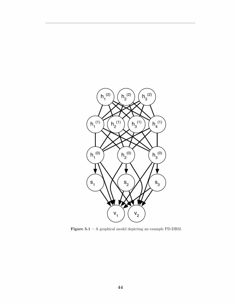
h1
(1) h2
(1) h3
(1)
h1
(0) h2
(0) h3
(0)
s1
s2
s3
v1
v2
h1
(2) h2
(2) h3
(2)
h4
(1)
Figure 5.1 – A graphical model depicting an example PD-DBM.
44
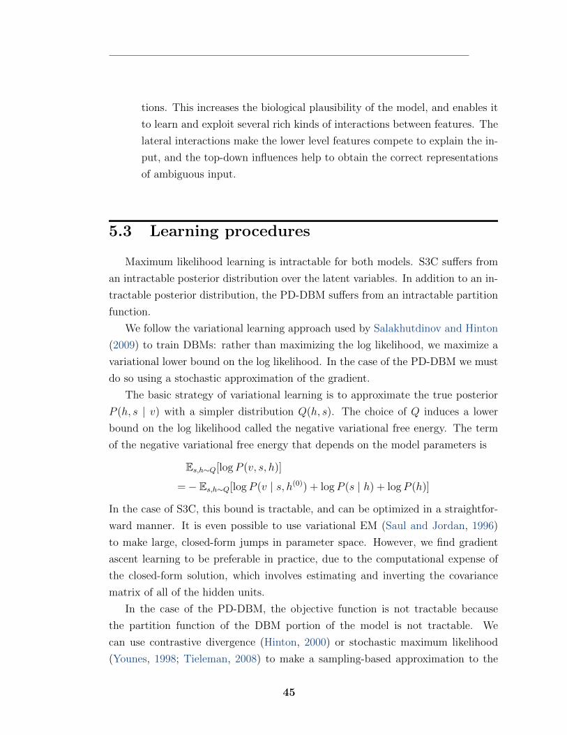
tions. This increases the biological plausibility of the model, and enables it
to learn and exploit several rich kinds of interactions between features. The
lateral interactions make the lower level features compete to explain the in-
put, and the top-down influences help to obtain the correct representations
of ambiguous input.
5.3 Learning procedures
Maximum likelihood learning is intractable for both models. S3C su↵ers from
an intractable posterior distribution over the latent variables. In addition to an in-
tractable posterior distribution, the PD-DBM su↵ers from an intractable partition
function.
We follow the variational learning approach used by Salakhutdinov and Hinton
(2009) to train DBMs: rather than maximizing the log likelihood, we maximize a
variational lower bound on the log likelihood. In the case of the PD-DBM we must
do so using a stochastic approximation of the gradient.
The basic strategy of variational learning is to approximate the true posterior
P (h, s | v) with a simpler distribution Q(h, s). The choice of Q induces a lower
bound on the log likelihood called the negative variational free energy. The term
of the negative variational free energy that depends on the model parameters is
Es,h⇠Q
[log P (v, s, h)]
= � Es,h⇠Q
[log P (v | s, h(0)) + log P (s | h) + log P (h)]
In the case of S3C, this bound is tractable, and can be optimized in a straightfor-
ward manner. It is even possible to use variational EM (Saul and Jordan, 1996)
to make large, closed-form jumps in parameter space. However, we find gradient
ascent learning to be preferable in practice, due to the computational expense of
the closed-form solution, which involves estimating and inverting the covariance
matrix of all of the hidden units.
In the case of the PD-DBM, the objective function is not tractable because
the partition function of the DBM portion of the model is not tractable. We
can use contrastive divergence (Hinton, 2000) or stochastic maximum likelihood
(Younes, 1998; Tieleman, 2008) to make a sampling-based approximation to the
45
DBM partition function’s contribution to the gradient. Thus, unlike S3C, we must
do gradient-based learning rather than closed-form parameter updates. However,
the PD-DBM model still has some nice properties in that only a subset of the
variables must be sampled during training. The factors of the partition function
originating from the S3C portion of the model are still tractable. In particular,
training does not ever require sampling real-valued variables. This is a nice property
because it means that the gradient estimates are bounded for fixed parameters and
data. When sampling real-valued variables, it is possible for the sampling procedure
to make gradient estimates arbitrarily large.
We found that using the “true gradient” (Douglas et al., 1999) method to be
useful for learning with the norm constraint on W . We also found that using
momentum (Hinton, 2010) is very important for learning PD-DBMs.
5.3.1 Avoiding greedy pretraining
Deep models are commonly pretrained in a greedy layerwise fashion. For ex-
ample, a DBM is usually initialized from a stack of RBMs, with one RBM trained
on the data and each of the other RBMs trained on samples of the previous RBM’s
hidden layer.
Any greedy training procedure can obviously get stuck in a local minimum.
Avoiding the need for greedy training could thus result in better models. For
example, when pretraining with an RBM, the lack of explaining away in the pos-
terior prevents the first layer from learning nearly parallel weight vectors, since
these would result in similar activations (up to the bias term, which could simply
make one unit always less active than the other). Even though the deeper layers
of the DBM could implement the explaining away needed for these weight vectors
to function correctly (ie, to have the one that resembles the input the most acti-
vate, and inhibit the other unit), the greedy learning procedure does not have the
opportunity to learn such weight vectors.
Previous e↵orts at jointly training even two layer DBMs on MNIST have failed
(Salakhutdinov and Hinton, 2009; Desjardins et al., 2012; Montavon and Muller,
2012). Typically, the jointly trained DBM does not make good use of the second
layer, either because the second layer weights are very small or because they contain
several duplicate weights focused on a small subset of first layer units that became
46
Figure 5.2 – This example histogram of EQ[hisi] shows that Q is a sparse distribution. For this6,000 hidden unit S3C model trained on 6 ⇥ 6 image patches, Q(hi = 1) < .01 99.7% of the time.
active early during training. We hypothesize that this is because the second layer
hidden units in a DBM must both learn to model correlations in the first layer
induced by the data and to counteract correlations in the first layer induced by the
model family. When the second layer weights are set to 0, the DBM prior acts to
correlate hidden units that have similar weight vectors (see Section 5.5.2).
The PD-DBM model avoids this problem. When the second layer weights are set
to 0, the first layer hidden units are independent in the PD-DBM prior (essentially
the S3C prior). The second layer thus has only one task: to model the correlations
between first layer units induced by the data. As we will show, this hypothesis is
supported by the fact that we are able to succesfully train a two layer PD-DBM
without greedy pre-training.
5.4 Inference procedures
The goal of variational inference is to maximize the lower bound on the log
likelihood with respect to the approximate distribution Q over the unobserved
variables. This is accomplished by selecting the Q that minimizes the Kullback–
Leibler divergence:
DKL
(Q(h, s)kP (h, s|v)) (5.2)
47
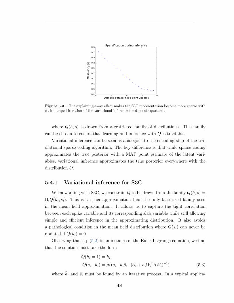
Figure 5.3 – The explaining-away e↵ect makes the S3C representation become more sparse witheach damped iteration of the variational inference fixed point equations.
where Q(h, s) is drawn from a restricted family of distributions. This family
can be chosen to ensure that learning and inference with Q is tractable.
Variational inference can be seen as analogous to the encoding step of the tra-
diational sparse coding algorithm. The key di↵erence is that while sparse coding
approximates the true posterior with a MAP point estimate of the latent vari-
ables, variational inference approximates the true posterior everywhere with the
distribution Q.
5.4.1 Variational inference for S3C
When working with S3C, we constrain Q to be drawn from the family Q(h, s) =
⇧i
Q(hi
, si
). This is a richer approximation than the fully factorized family used
in the mean field approximation. It allows us to capture the tight correlation
between each spike variable and its corresponding slab variable while still allowing
simple and e�cient inference in the approximating distribution. It also avoids
a pathological condition in the mean field distribution where Q(si
) can never be
updated if Q(hi
) = 0.
Observing that eq. (5.2) is an instance of the Euler-Lagrange equation, we find
that the solution must take the form
Q(hi
= 1) = hi
,
Q(si
| hi
) = N (si
| hi
si
, (↵i
+ hi
W>i
�Wi
)�1) (5.3)
where hi
and si
must be found by an iterative process. In a typical applica-
48
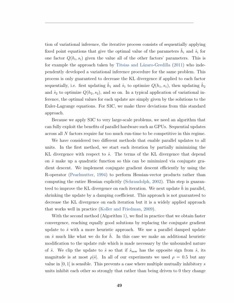
tion of variational inference, the iterative process consists of sequentially applying
fixed point equations that give the optimal value of the parameters hi
and si
for
one factor Q(hi
, si
) given the value all of the other factors’ parameters. This is
for example the approach taken by Titsias and Lazaro-Gredilla (2011) who inde-
pendently developed a variational inference procedure for the same problem. This
process is only guaranteed to decrease the KL divergence if applied to each factor
sequentially, i.e. first updating h1
and s1
to optimize Q(h1
, s1
), then updating h2
and s2
to optimize Q(h2
, s2
), and so on. In a typical application of variational in-
ference, the optimal values for each update are simply given by the solutions to the
Euler-Lagrange equations. For S3C, we make three deviations from this standard
approach.
Because we apply S3C to very large-scale problems, we need an algorithm that
can fully exploit the benefits of parallel hardware such as GPUs. Sequential updates
across all N factors require far too much run-time to be competitive in this regime.
We have considered two di↵erent methods that enable parallel updates to all
units. In the first method, we start each iteration by partially minimizing the
KL divergence with respect to s. The terms of the KL divergence that depend
on s make up a quadratic function so this can be minimized via conjugate gra-
dient descent. We implement conjugate gradient descent e�ciently by using the
R-operator (Pearlmutter, 1994) to perform Hessian-vector products rather than
computing the entire Hessian explicitly (Schraudolph, 2002). This step is guaran-
teed to improve the KL divergence on each iteration. We next update h in parallel,
shrinking the update by a damping coe�cient. This approach is not guaranteed to
decrease the KL divergence on each iteration but it is a widely applied approach
that works well in practice (Koller and Friedman, 2009).
With the second method (Algorithm 1), we find in practice that we obtain faster
convergence, reaching equally good solutions by replacing the conjugate gradient
update to s with a more heuristic approach. We use a parallel damped update
on s much like what we do for h. In this case we make an additional heuristic
modification to the update rule which is made necessary by the unbounded nature
of s. We clip the update to s so that if snew
has the opposite sign from s, its
magnitude is at most ⇢|s|. In all of our experiments we used ⇢ = 0.5 but any
value in [0, 1] is sensible. This prevents a case where multiple mutually inhibitory s
units inhibit each other so strongly that rather than being driven to 0 they change
49
sign and actually increase in magnitude. This case is a failure mode of the parallel
updates that can result in s amplifying without bound if clipping is not used.
Note that Algorithm 1 does not specify a convergence criterion. Many conver-
gence criteria are possible–the convergence criterion could be based on the norm of
the gradient of the KL divergence with respect to the variational parameters, the
amount that the KL divergence has decreased in the last iteration, or the amount
that the variational parameters have changed in the final iteration. Salakhutdinov
and Hinton (2009) use the third approach when training deep Boltzmann machines
and we find that it works well for S3C and the PD-DBM as well.
Algorithm 1 Fixed-Point Inference
Initialize
ˆh(0) = �(b), s(0) = µ, and k = 0.
while not converged do
Compute the individually optimal value s⇤i for each i simultaneously:
s⇤i =
µi↵ii + v>�Wi �Wi�hP
j 6=i Wjˆhj sj(k)
i
↵ii + W>i �Wi
Clip reflections by assigning
ci = ⇢sign(s⇤i )|si(k)|
for all i such that sign(s⇤i ) 6= sign(si(k)) and |s⇤i | > ⇢|si(k)|, and assigning ci = s⇤i for all other i.Damp the updates by assigning
s(k + 1)i = ⌘sc + (1� ⌘s)s(k)
where ⌘s 2 (0, 1].
Compute the individually optimal values for
ˆh:
zi =
0
@v �X
j 6=i
Wj sj(k + 1)
ˆhj(k)�1
2
Wisi(k + 1)
1
A>
�Wisi(k + 1) + bi �1
2
↵ii(si(k + 1)� µi)2 �
1
2
log(↵ii + W>i �Wi) +
1
2
log(↵ii)
ˆh⇤i = �(z)
Damp the update to
ˆh:
ˆh(k + 1) = ⌘hˆh⇤
+ (1� ⌘h)
ˆh(k)
k k + 1
end while
We include some visualizations that demonstrate the e↵ect of our inference
procedure. Figure 5.2 shows that it produces a sparse representation. Figure
5.3 shows that the explaining-away e↵ect incrementally makes the representation
more sparse. Figure 5.4 shows that the inference procedure increases the negative
variational free energy.
50
Figure 5.4 – The negative variational free energy of a batch of 5000 image patches increasesduring the course of variational inference.
5.4.2 Variational inference for the PD-DBM
Inference in the PD-DBM is very similar to inference in S3C. We use the vari-
ational family
Q(s, h) = ⇧N
0
i=1
Q(si
, h(0)
i
)⇧L
l=1
⇧Nli=1
Q(h(l)
i
)
whose solutions take the form
Q(h(l)
i
= 1) = h(l)
i
,
Q(si
| h(0)
i
) = N (si
| h(0)
i
si
, (↵i
+ hi
W>i
�Wi
)�1).
We apply more or less the same inference procedure as in S3C. On each update
step we update either s or h(l) for some value of l. The update to s is exactly the
same as in S3C. The update to h(0) changes slightly to incorporate top-down influ-
ence from h(1). When computing the individually optimal values of the elements
of h(0) we use the following fixed-point formula:
h(0)⇤i
= �(zi
+ W (1)h(1))
The update to h(l) for l > 0 is simple; it is the same as the mean field update in
the DBM. No damping is necessary for this update. The conditional independence
properties of the DBM guarantee that the optimal values of the elements of h(l) do
not depend on each other, so the individually optimal values are globally optimal
(for a given h(l�1) and h(l+1)). The update is given by
h(l)⇤ = �⇣b(l) + h(l�1)T W (l) + W (l+1)h(l+1)
⌘
where the term for layer l + 1 is dropped if l + 1 > L.
51
5.5 Comparison to other feature encoding
methods
Here we compare S3C as a feature discovery algorithm to other popular ap-
proaches. We describing how S3C occupies a middle ground between two of these
methods, sparse coding and the ssRBM, while avoiding many of the respective
disadvantages when applied as feature discovery algorithms.
5.5.1 Comparison to sparse coding
Sparse coding (Olshausen and Field, 1997) has been widely used to discover
features for classification (Raina et al., 2007). Recently Coates and Ng (2011)
showed that this approach achieves excellent performance on the CIFAR-10 object
recognition dataset. Sparse coding refers to a class of generative models where the
observed data v is normally distributed given a set of continuous latent variables
s and a dictionary matrix W : v ⇠ N (Ws, �I). Sparse coding places a factorial
and heavy tailed prior distribution over s (e.g. a Cauchy or Laplace distribution)
chosen to encourage the mode of the posterior p(s | v) to be sparse. One can derive
the S3C model from sparse coding by replacing the factorial Cauchy or Laplace
prior with a spike-and-slab prior.
One drawback of sparse coding is that the latent variables are not merely en-
couraged to be sparse; they are encouraged to remain close to 0, even when they
are active. This kind of regularization is not necessarily undesirable, but in the
case of simple but popular priors such as the Laplace prior (corresponding to an
L1
penalty on the latent variables s), the degree of regularization on active units
is confounded with the degree of sparsity. There is little reason to believe that in
realistic settings, these two types of complexity control should be so tightly bound
together. The S3C model avoids this issue by controlling the sparsity of units via
the b parameter that determines how likely each spike unit is to be active, while
separately controlling the magnitude of active units via the µ and ↵ parameters
that govern the distribution over s. Sparse coding has no parameter analogous to
µ and cannot control these aspects of the posterior independently.
Another drawback of sparse coding is that the factors are not actually sparse in
the generative distribution. Indeed, each factor is zero with probability zero. The
52
features extracted by sparse coding are only sparse because they are obtained via
MAP inference. In the S3C model, the spike variables ensure that each factor is
zero with non-zero probability in the generative distribution. Since this places a
greater restriction on the code variables, we hypothesize that S3C features provide
more of a regularizing e↵ect when solving classification problems.
Sparse coding is also di�cult to integrate into a deep generative model of data
such as natural images. While Yu et al. (2011) and Zeiler et al. (2011) have recently
shown some success at learning hierarchical sparse coding, our goal is to integrate
the feature extraction scheme into a proven generative model framework such as
the deep Boltzmann machine (Salakhutdinov and Hinton, 2009). Existing inference
schemes known to work well in the DBM-type (deep Boltzmann machine) setting
are all either sample-based or are based on variational approximations to the model
posteriors, while sparse coding schemes typically employ MAP inference. Our use
of variational inference makes the S3C framework well suited to integrate into the
known successful strategies for learning and inference in DBM models. In fact,
the compatibility of the S3C and DBM inference procedures is confirmed by the
success of the PD-DBM inference procedure. It is not obvious how one can employ
a variational inference strategy to standard sparse coding with the goal of achieving
sparse feature encoding.
Sparse coding models can be learned e�ciently by alternately running MAP
inference for several examples and then making a large, closed-form updates to
the parameters. The same approach is also possible with S3C, and is in fact more
principled since it is based on maximizing a variational lower bound rather than
the MAP approximation. We do not explore this learning method for S3C in this
paper.
5.5.2 Comparison to restricted Boltzmann machines
The S3C model also resembles another class of models commonly used for fea-
ture discovery: the RBM. An RBM (Smolensky, 1986) is a model defined through
an energy function that describes the interactions between the observed data vari-
ables and a set of latent variables. It is possible to interpret the S3C as an energy-
based model, by rearranging p(v, s, h) to take the form exp{�E(v, s, h)}/Z, with
53
the following energy function:
E(v, s, h) =1
2
v �
X
i
Wi
si
hi
!>
�
v �
X
i
Wi
si
hi
!
+1
2
NX
i=1
↵i
(si
� µi
hi
)2 �NX
i=1
bi
hi
, (5.4)
The ssRBM model family is a good starting point for S3C because it has demon-
strated both reasonable performance as a feature discovery scheme and remarkable
performance as a generative model (Courville et al., 2011b). Within the ssRBM
family, S3C’s closest relative is a variant of the µ-ssRBM, defined by the following
energy function:
E(v, s, h) = �NX
i=1
vT �Wi
si
hi
+1
2vT �v
+1
2
NX
i=1
↵i
(si
� µi
hi
)2 �NX
i=1
bi
hi
, (5.5)
where the variables and parameters are defined identically to those in S3C. Com-
parison of equations 5.4 and 5.5 reveals that the simple addition of a latent factor
interaction term 1
2
(h � s)>W>�W (h � s) to the ssRBM energy function turns the
ssRBM into the S3C model. With the inclusion of this term S3C moves from
an undirected ssRBM model to the directed graphical model described in equa-
tion (5.1). This change from undirected modeling to directed modeling has three
important e↵ects, that we describe in the following paragraphs:
The e↵ect on the partition function: The most immediate consequence of
the transition to directed modeling is that the partition function becomes tractable.
Because the RBM parition function is intractable, most training algorithms for the
RBM require making stochastic approximations to the partition function, the same
as our learning procedure for the PD-DBM does. Since the S3C partition function
is tractable, we can follow its true gradient, which provides one advantage over
the RBM. The partition function of S3C is also guaranteed to exist for all possible
settings of the model parameters, which is not true of the ssRBM. In the ssRBM,
for some parameter values, it is possible for p(s, v | h) to take the form of a normal
distribution whose covariance matrix is not positive definite. Courville et al.
(2011b) have explored resolving this issue by constraining the parameters, but this
54
was found to hurt classification performance.
The e↵ect on the posterior: RBMs have a factorial posterior, but S3C
and sparse coding have a complicated posterior due to the “explaining away” e↵ect.
For this reason, RBMs can use exact inference and maximum likelihood estimation.
Models with an intractable posterior such as S3C and DBMs must use approximate
inference and are often trained with a variational lower bound on the likelihood.
The RBMs factorial posterior means that features defined by similar basis func-
tions will have similar activations, while in directed models, similar features will
compete so that only the most relevant features will remain significantly active.
As shown by Coates and Ng (2011), the sparse Gaussian RBM is not a very good
feature extractor – the set of basis functions W learned by the RBM actually work
better for supervised learning when these parameters are plugged into a sparse
coding model than when the RBM itself is used for feature extraction. We think
this is due to the factorial posterior. In the vastly overcomplete setting, being able
to selectively activate a small set of features that cooperate to explain the input
likely provides S3C a major advantage in discriminative capability.
Considerations of biological plausibility also motivate the use of a model with
a complicated posterior. As described in (Hyvarinen et al., 2009), a phenomenon
called “end stopping” similar to explaining away has been observed in V1 simple
cells. End-stopping occurs when an edge detector is inhibited when retinal cells
near the ends of the edge it detects are stimulated. The inhibition occurs due to
lateral interactions with other simple cells, and is a major motivation for the lateral
interactions present in the sparse coding posterior.
The e↵ect on the prior: The addition of the interaction term causes S3C
to have a factorial prior. This probably makes it a poor generative model, but this
is not a problem for the purpose of feature discovery. Moreover, the quality of the
generative model can be improved by incorporating S3C into a deeper architecture,
as we will show.
RBMs were designed with a nonfactorial prior because factor models with fac-
torial priors are generally known to result in poor generative models. However,
in the case of real-valued data, typical RBM priors are not especially useful. For
55
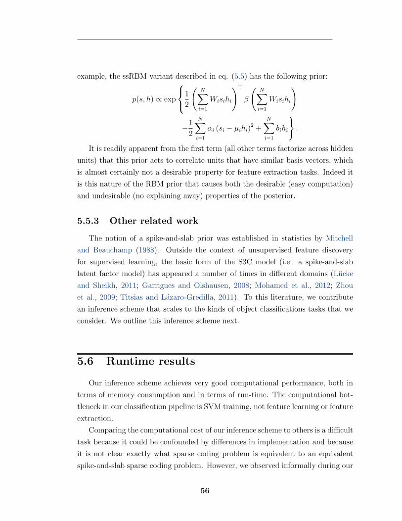
example, the ssRBM variant described in eq. (5.5) has the following prior:
p(s, h) / exp
8<
:1
2
NX
i=1
Wi
si
hi
!>
�
NX
i=1
Wi
si
hi
!
�1
2
NX
i=1
↵i
(si
� µi
hi
)2 +NX
i=1
bi
hi
).
It is readily apparent from the first term (all other terms factorize across hidden
units) that this prior acts to correlate units that have similar basis vectors, which
is almost certainly not a desirable property for feature extraction tasks. Indeed it
is this nature of the RBM prior that causes both the desirable (easy computation)
and undesirable (no explaining away) properties of the posterior.
5.5.3 Other related work
The notion of a spike-and-slab prior was established in statistics by Mitchell
and Beauchamp (1988). Outside the context of unsupervised feature discovery
for supervised learning, the basic form of the S3C model (i.e. a spike-and-slab
latent factor model) has appeared a number of times in di↵erent domains (Lucke
and Sheikh, 2011; Garrigues and Olshausen, 2008; Mohamed et al., 2012; Zhou
et al., 2009; Titsias and Lazaro-Gredilla, 2011). To this literature, we contribute
an inference scheme that scales to the kinds of object classifications tasks that we
consider. We outline this inference scheme next.
5.6 Runtime results
Our inference scheme achieves very good computational performance, both in
terms of memory consumption and in terms of run-time. The computational bot-
tleneck in our classification pipeline is SVM training, not feature learning or feature
extraction.
Comparing the computational cost of our inference scheme to others is a di�cult
task because it could be confounded by di↵erences in implementation and because
it is not clear exactly what sparse coding problem is equivalent to an equivalent
spike-and-slab sparse coding problem. However, we observed informally during our
56
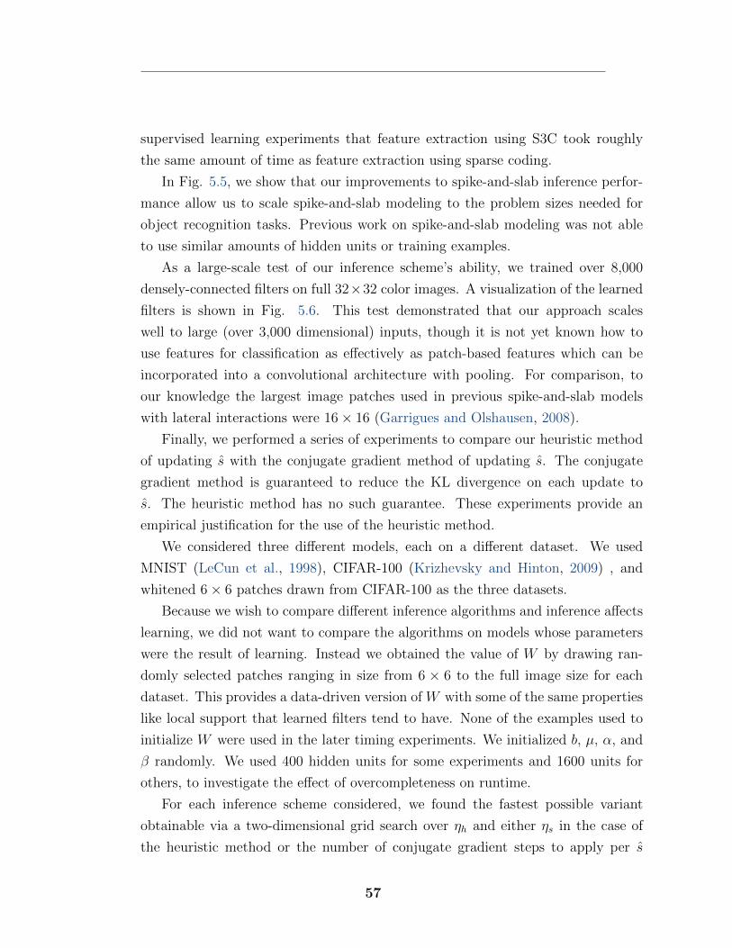
supervised learning experiments that feature extraction using S3C took roughly
the same amount of time as feature extraction using sparse coding.
In Fig. 5.5, we show that our improvements to spike-and-slab inference perfor-
mance allow us to scale spike-and-slab modeling to the problem sizes needed for
object recognition tasks. Previous work on spike-and-slab modeling was not able
to use similar amounts of hidden units or training examples.
As a large-scale test of our inference scheme’s ability, we trained over 8,000
densely-connected filters on full 32⇥32 color images. A visualization of the learned
filters is shown in Fig. 5.6. This test demonstrated that our approach scales
well to large (over 3,000 dimensional) inputs, though it is not yet known how to
use features for classification as e↵ectively as patch-based features which can be
incorporated into a convolutional architecture with pooling. For comparison, to
our knowledge the largest image patches used in previous spike-and-slab models
with lateral interactions were 16 ⇥ 16 (Garrigues and Olshausen, 2008).
Finally, we performed a series of experiments to compare our heuristic method
of updating s with the conjugate gradient method of updating s. The conjugate
gradient method is guaranteed to reduce the KL divergence on each update to
s. The heuristic method has no such guarantee. These experiments provide an
empirical justification for the use of the heuristic method.
We considered three di↵erent models, each on a di↵erent dataset. We used
MNIST (LeCun et al., 1998), CIFAR-100 (Krizhevsky and Hinton, 2009) , and
whitened 6 ⇥ 6 patches drawn from CIFAR-100 as the three datasets.
Because we wish to compare di↵erent inference algorithms and inference a↵ects
learning, we did not want to compare the algorithms on models whose parameters
were the result of learning. Instead we obtained the value of W by drawing ran-
domly selected patches ranging in size from 6 ⇥ 6 to the full image size for each
dataset. This provides a data-driven version of W with some of the same properties
like local support that learned filters tend to have. None of the examples used to
initialize W were used in the later timing experiments. We initialized b, µ, ↵, and
� randomly. We used 400 hidden units for some experiments and 1600 units for
others, to investigate the e↵ect of overcompleteness on runtime.
For each inference scheme considered, we found the fastest possible variant
obtainable via a two-dimensional grid search over ⌘h
and either ⌘s
in the case of
the heuristic method or the number of conjugate gradient steps to apply per s
57
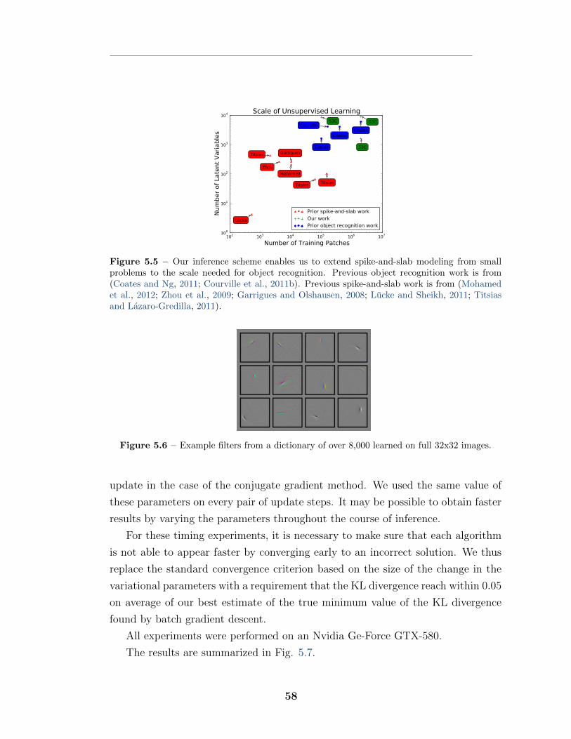
Figure 5.5 – Our inference scheme enables us to extend spike-and-slab modeling from smallproblems to the scale needed for object recognition. Previous object recognition work is from(Coates and Ng, 2011; Courville et al., 2011b). Previous spike-and-slab work is from (Mohamedet al., 2012; Zhou et al., 2009; Garrigues and Olshausen, 2008; Lucke and Sheikh, 2011; Titsiasand Lazaro-Gredilla, 2011).
Figure 5.6 – Example filters from a dictionary of over 8,000 learned on full 32x32 images.
update in the case of the conjugate gradient method. We used the same value of
these parameters on every pair of update steps. It may be possible to obtain faster
results by varying the parameters throughout the course of inference.
For these timing experiments, it is necessary to make sure that each algorithm
is not able to appear faster by converging early to an incorrect solution. We thus
replace the standard convergence criterion based on the size of the change in the
variational parameters with a requirement that the KL divergence reach within 0.05
on average of our best estimate of the true minimum value of the KL divergence
found by batch gradient descent.
All experiments were performed on an Nvidia Ge-Force GTX-580.
The results are summarized in Fig. 5.7.
58
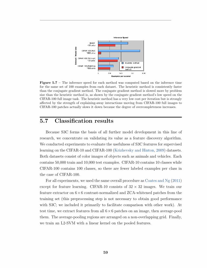
Figure 5.7 – The inference speed for each method was computed based on the inference timefor the same set of 100 examples from each dataset. The heuristic method is consistently fasterthan the conjugate gradient method. The conjugate gradient method is slowed more by problemsize than the heuristic method is, as shown by the conjugate gradient method’s low speed on theCIFAR-100 full image task. The heuristic method has a very low cost per iteration but is stronglya↵ected by the strength of explaining-away interactions–moving from CIFAR-100 full images toCIFAR-100 patches actually slows it down because the degree of overcompleteness increases.
5.7 Classification results
Because S3C forms the basis of all further model development in this line of
research, we concentrate on validating its value as a feature discovery algorithm.
We conducted experiments to evaluate the usefulness of S3C features for supervised
learning on the CIFAR-10 and CIFAR-100 (Krizhevsky and Hinton, 2009) datasets.
Both datasets consist of color images of objects such as animals and vehicles. Each
contains 50,000 train and 10,000 test examples. CIFAR-10 contains 10 classes while
CIFAR-100 contains 100 classes, so there are fewer labeled examples per class in
the case of CIFAR-100.
For all experiments, we used the same overall procedure as Coates and Ng (2011)
except for feature learning. CIFAR-10 consists of 32 ⇥ 32 images. We train our
feature extractor on 6⇥6 contrast-normalized and ZCA-whitened patches from the
training set (this preprocessing step is not necessary to obtain good performance
with S3C; we included it primarily to facilitate comparison with other work). At
test time, we extract features from all 6⇥6 patches on an image, then average-pool
them. The average-pooling regions are arranged on a non-overlapping grid. Finally,
we train an L2-SVM with a linear kernel on the pooled features.
59
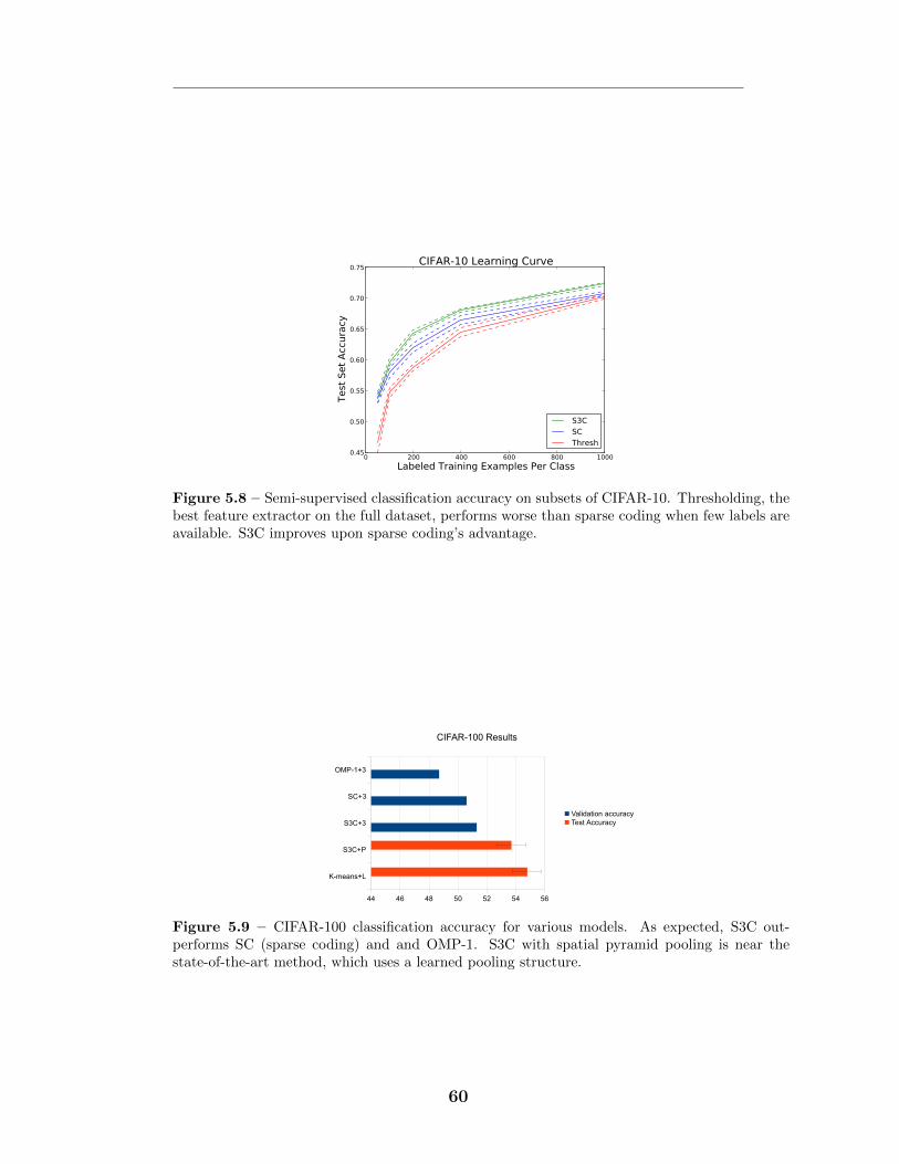
Figure 5.8 – Semi-supervised classification accuracy on subsets of CIFAR-10. Thresholding, thebest feature extractor on the full dataset, performs worse than sparse coding when few labels areavailable. S3C improves upon sparse coding’s advantage.
Sheet1
Page 1
Model Validation accuracyTest Accuracy ErrorK-means+L 54.8 1S3C+P 53.7 1S3C+3 51.3SC+3 50.6OMP-1+3 48.7
K-means+L
S3C+P
S3C+3
SC+3
OMP-1+3
44 46 48 50 52 54 56
CIFAR-100 Results
Validation accuracy
Test Accuracy
Figure 5.9 – CIFAR-100 classification accuracy for various models. As expected, S3C out-performs SC (sparse coding) and and OMP-1. S3C with spatial pyramid pooling is near thestate-of-the-art method, which uses a learned pooling structure.
60
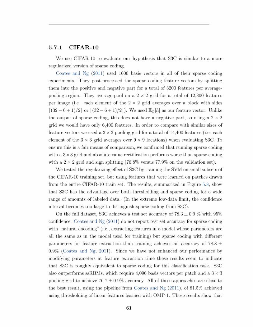
5.7.1 CIFAR-10
We use CIFAR-10 to evaluate our hypothesis that S3C is similar to a more
regularized version of sparse coding.
Coates and Ng (2011) used 1600 basis vectors in all of their sparse coding
experiments. They post-processed the sparse coding feature vectors by splitting
them into the positive and negative part for a total of 3200 features per average-
pooling region. They average-pool on a 2 ⇥ 2 grid for a total of 12,800 features
per image (i.e. each element of the 2 ⇥ 2 grid averages over a block with sides
d(32 � 6 + 1)/2e or b(32 � 6 + 1)/2c). We used EQ
[h] as our feature vector. Unlike
the output of sparse coding, this does not have a negative part, so using a 2 ⇥ 2
grid we would have only 6,400 features. In order to compare with similar sizes of
feature vectors we used a 3 ⇥ 3 pooling grid for a total of 14,400 features (i.e. each
element of the 3 ⇥ 3 grid averages over 9 ⇥ 9 locations) when evaluating S3C. To
ensure this is a fair means of comparison, we confirmed that running sparse coding
with a 3⇥3 grid and absolute value rectification performs worse than sparse coding
with a 2 ⇥ 2 grid and sign splitting (76.8% versus 77.9% on the validation set).
We tested the regularizing e↵ect of S3C by training the SVM on small subsets of
the CIFAR-10 training set, but using features that were learned on patches drawn
from the entire CIFAR-10 train set. The results, summarized in Figure 5.8, show
that S3C has the advantage over both thresholding and sparse coding for a wide
range of amounts of labeled data. (In the extreme low-data limit, the confidence
interval becomes too large to distinguish sparse coding from S3C).
On the full dataset, S3C achieves a test set accuracy of 78.3 ± 0.9 % with 95%
confidence. Coates and Ng (2011) do not report test set accuracy for sparse coding
with “natural encoding” (i.e., extracting features in a model whose parameters are
all the same as in the model used for training) but sparse coding with di↵erent
parameters for feature extraction than training achieves an accuracy of 78.8 ±0.9% (Coates and Ng, 2011). Since we have not enhanced our performance by
modifying parameters at feature extraction time these results seem to indicate
that S3C is roughly equivalent to sparse coding for this classification task. S3C
also outperforms ssRBMs, which require 4,096 basis vectors per patch and a 3 ⇥ 3
pooling grid to achieve 76.7 ± 0.9% accuracy. All of these approaches are close to
the best result, using the pipeline from Coates and Ng (2011), of 81.5% achieved
using thresholding of linear features learned with OMP-1. These results show that
61
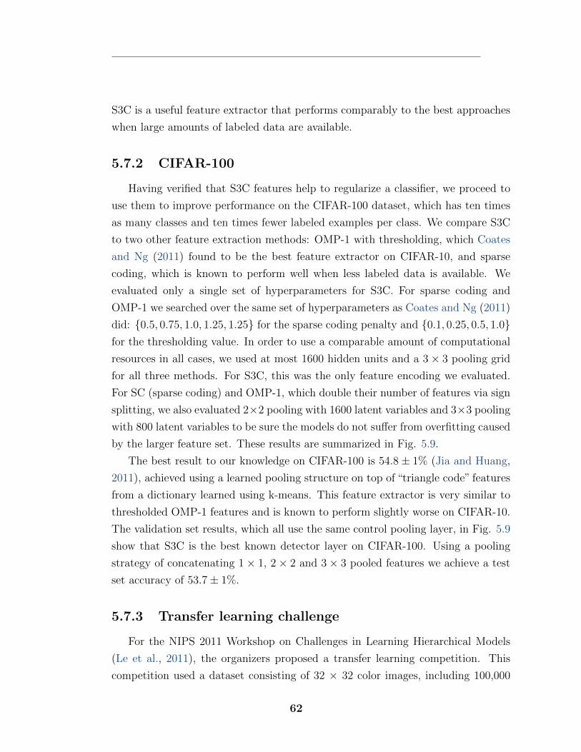
S3C is a useful feature extractor that performs comparably to the best approaches
when large amounts of labeled data are available.
5.7.2 CIFAR-100
Having verified that S3C features help to regularize a classifier, we proceed to
use them to improve performance on the CIFAR-100 dataset, which has ten times
as many classes and ten times fewer labeled examples per class. We compare S3C
to two other feature extraction methods: OMP-1 with thresholding, which Coates
and Ng (2011) found to be the best feature extractor on CIFAR-10, and sparse
coding, which is known to perform well when less labeled data is available. We
evaluated only a single set of hyperparameters for S3C. For sparse coding and
OMP-1 we searched over the same set of hyperparameters as Coates and Ng (2011)
did: {0.5, 0.75, 1.0, 1.25, 1.25} for the sparse coding penalty and {0.1, 0.25, 0.5, 1.0}for the thresholding value. In order to use a comparable amount of computational
resources in all cases, we used at most 1600 hidden units and a 3 ⇥ 3 pooling grid
for all three methods. For S3C, this was the only feature encoding we evaluated.
For SC (sparse coding) and OMP-1, which double their number of features via sign
splitting, we also evaluated 2⇥2 pooling with 1600 latent variables and 3⇥3 pooling
with 800 latent variables to be sure the models do not su↵er from overfitting caused
by the larger feature set. These results are summarized in Fig. 5.9.
The best result to our knowledge on CIFAR-100 is 54.8 ± 1% (Jia and Huang,
2011), achieved using a learned pooling structure on top of “triangle code” features
from a dictionary learned using k-means. This feature extractor is very similar to
thresholded OMP-1 features and is known to perform slightly worse on CIFAR-10.
The validation set results, which all use the same control pooling layer, in Fig. 5.9
show that S3C is the best known detector layer on CIFAR-100. Using a pooling
strategy of concatenating 1 ⇥ 1, 2 ⇥ 2 and 3 ⇥ 3 pooled features we achieve a test
set accuracy of 53.7 ± 1%.
5.7.3 Transfer learning challenge
For the NIPS 2011 Workshop on Challenges in Learning Hierarchical Models
(Le et al., 2011), the organizers proposed a transfer learning competition. This
competition used a dataset consisting of 32 ⇥ 32 color images, including 100,000
62
Sheet1
Page 1
S3C, E[h], 6000 units 68.8 1.1S3C, E[h] 68.4 1.1S3C, random patches 67.7 1.1S3C, MAP h under Q 66.6 1.1S3C, E[h], zero mean 66.4 1.1S3C, mu=0, alpha=1e6 66.3 1.1
S3C, E[h], 6000 units
S3C, E[h]
S3C, random patches
S3C, MAP h under Q
S3C, E[h], zero mean
S3C, mu=0, alpha=1e6
64 65 66 67 68 69 70
Ablative Analysis
Test Set Accuracy (Percent)
Figure 5.10 – Performance of several limited variants of S3C
unlabeled examples, 50,000 labeled examples of 100 object classes not present in
the test set, and 120 labeled examples of 10 object classes present in the test set.
The test set was not made public until after the competition. We recognized this
contest as a chance to demonstrate S3C’s ability to perform well with extremely
small amounts of labeled data. We chose to disregard the 50,000 labels and treat
this as a semi-supervised learning task.
We applied the same approach as on the CIFAR datasets, albeit with a small
modification to the SVM training procedure. Due to the small labeled dataset size,
we used leave-one-out cross validation rather than five fold cross validation.
We won the competition, with a test set accuracy of 48.6 %. We do not have
any information about the competing entries, other than that we outperformed
them. Our test set accuracy was tied with a method run by the contest organizers,
based on a combination of methods (Coates et al., 2011; Le et al., 2011). Since
these methods do not use transfer learning either, this suggests that the contest
primarily provides evidence that S3C is a powerful semi-supervised learning tool.
5.7.4 Ablative analysis
In order to better understand which aspects of our S3C object classification
method are most important to obtaining good performance, we conducted a series
of ablative analysis experiments. For these experiments we trained on 5,000 labels
of the STL-10 dataset (Coates et al., 2011). Previous work on the STL-10 dataset
is based on training on 1,000 label subsets of the training set, so the performance
numbers in this section should only be compared to each other, not to previous
work. The results are presented in Fig. 5.10.
63
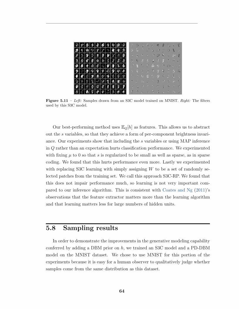
Figure 5.11 – Left: Samples drawn from an S3C model trained on MNIST. Right: The filtersused by this S3C model.
Our best-performing method uses EQ
[h] as features. This allows us to abstract
out the s variables, so that they achieve a form of per-component brightness invari-
ance. Our experiments show that including the s variables or using MAP inference
in Q rather than an expectation hurts classification performance. We experimented
with fixing µ to 0 so that s is regularized to be small as well as sparse, as in sparse
coding. We found that this hurts performance even more. Lastly we experimented
with replacing S3C learning with simply assigning W to be a set of randomly se-
lected patches from the training set. We call this approach S3C-RP. We found that
this does not impair performance much, so learning is not very important com-
pared to our inference algorithm. This is consistent with Coates and Ng (2011)’s
observations that the feature extractor matters more than the learning algorithm
and that learning matters less for large numbers of hidden units.
5.8 Sampling results
In order to demonstrate the improvements in the generative modeling capability
conferred by adding a DBM prior on h, we trained an S3C model and a PD-DBM
model on the MNIST dataset. We chose to use MNIST for this portion of the
experiments because it is easy for a human observer to qualitatively judge whether
samples come from the same distribution as this dataset.
64
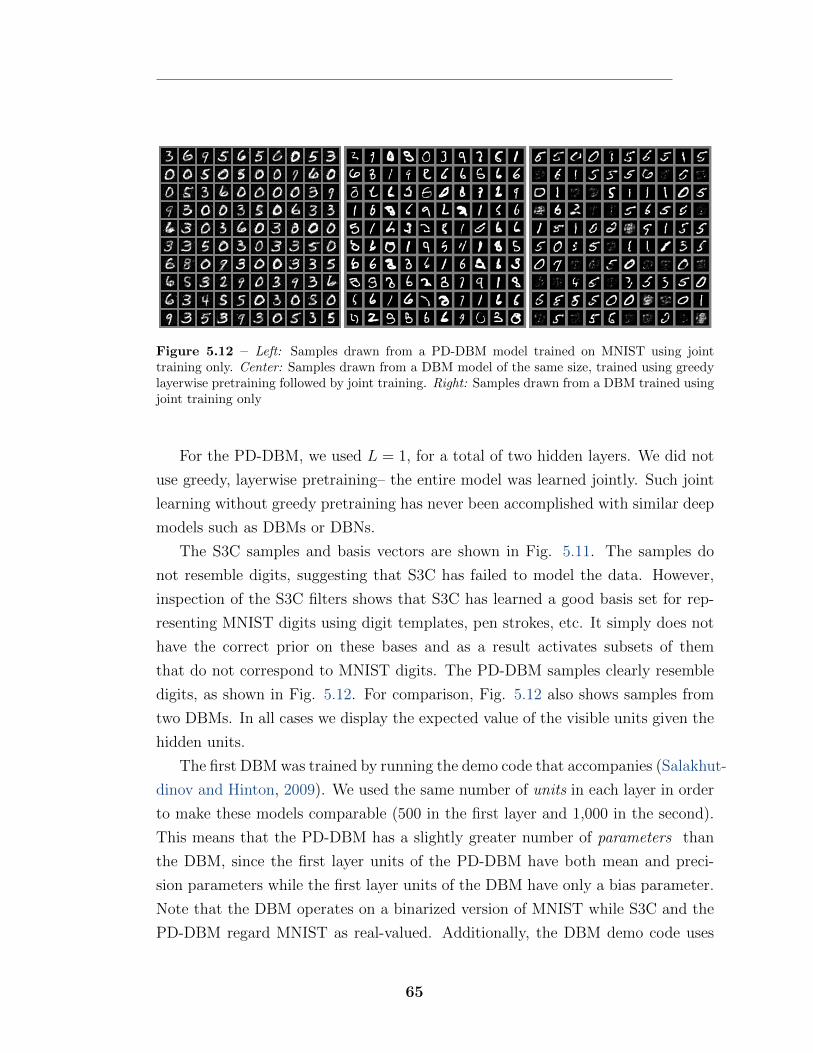
Figure 5.12 – Left: Samples drawn from a PD-DBM model trained on MNIST using jointtraining only. Center: Samples drawn from a DBM model of the same size, trained using greedylayerwise pretraining followed by joint training. Right: Samples drawn from a DBM trained usingjoint training only
For the PD-DBM, we used L = 1, for a total of two hidden layers. We did not
use greedy, layerwise pretraining– the entire model was learned jointly. Such joint
learning without greedy pretraining has never been accomplished with similar deep
models such as DBMs or DBNs.
The S3C samples and basis vectors are shown in Fig. 5.11. The samples do
not resemble digits, suggesting that S3C has failed to model the data. However,
inspection of the S3C filters shows that S3C has learned a good basis set for rep-
resenting MNIST digits using digit templates, pen strokes, etc. It simply does not
have the correct prior on these bases and as a result activates subsets of them
that do not correspond to MNIST digits. The PD-DBM samples clearly resemble
digits, as shown in Fig. 5.12. For comparison, Fig. 5.12 also shows samples from
two DBMs. In all cases we display the expected value of the visible units given the
hidden units.
The first DBM was trained by running the demo code that accompanies (Salakhut-
dinov and Hinton, 2009). We used the same number of units in each layer in order
to make these models comparable (500 in the first layer and 1,000 in the second).
This means that the PD-DBM has a slightly greater number of parameters than
the DBM, since the first layer units of the PD-DBM have both mean and preci-
sion parameters while the first layer units of the DBM have only a bias parameter.
Note that the DBM operates on a binarized version of MNIST while S3C and the
PD-DBM regard MNIST as real-valued. Additionally, the DBM demo code uses
65
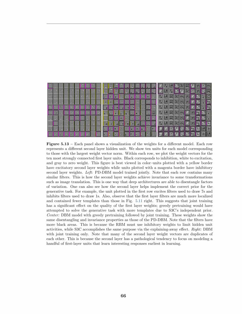
Figure 5.13 – Each panel shows a visualization of the weights for a di↵erent model. Each rowrepresents a di↵erent second layer hidden unit. We show ten units for each model correspondingto those with the largest weight vector norm. Within each row, we plot the weight vectors for theten most strongly connected first layer units. Black corresponds to inhibition, white to excitation,and gray to zero weight. This figure is best viewed in color–units plotted with a yellow borderhave excitatory second layer weights while units plotted with a magenta border have inhibitorysecond layer weights. Left: PD-DBM model trained jointly. Note that each row contains manysimilar filters. This is how the second layer weights achieve invariance to some transformationssuch as image translation. This is one way that deep architectures are able to disentangle factorsof variation. One can also see how the second layer helps implement the correct prior for thegenerative task. For example, the unit plotted in the first row excites filters used to draw 7s andinhibits filters used to draw 1s. Also, observe that the first layer filters are much more localizedand contained fewer templates than those in Fig. 5.11 right. This suggests that joint traininghas a significant e↵ect on the quality of the first layer weights; greedy pretraining would haveattempted to solve the generative task with more templates due to S3C’s independent prior.Center: DBM model with greedy pretraining followed by joint training. These weights show thesame disentangling and invariance properties as those of the PD-DBM. Note that the filters havemore black areas. This is because the RBM must use inhibitory weights to limit hidden unitactivities, while S3C accomplishes the same purpose via the explaining-away e↵ect. Right: DBMwith joint training only. Note that many of the second layer weight vectors are duplicates ofeach other. This is because the second layer has a pathological tendency to focus on modeling ahandful of first-layer units that learn interesting responses earliest in learning.
66
the MNIST labels during generative training while the PD-DBM and S3C were
not trained with the benefit of the labels. The DBM demo code is hardcoded to
pretrain the first layer for 100 epochs, the second layer for 200 epochs, and then
jointly train the DBM for 300 epochs. We trained the PD-DBM starting from a
random initialization for 350 epochs.
The second DBM was trained using two modifications from the demo code
in order to train it in as similar a fashion to our PD-DBM model as possible:
first, it was trained without access to labels, and second, it did not receive any
pretraining. This model was trained for only 230 epochs because it had already
converged to a bad local optimum by this time. This DBM is included to provide an
example of how DBM training fails when greedy layerwise pretraining is not used.
DBM training can fail in a variety of ways and no example should be considered
representative of all of them.
To analyze the di↵erences between these models, we display a visualization of
the weights of the models that shows how the layers interact in Fig. 5.13.
5.9 Conclusion
We have motivated the use of the S3C model for unsupervised feature discov-
ery. We have described a variational approximation scheme that makes it feasible
to perform learning and inference in large-scale S3C and PD-DBM models. We
have demonstrated that S3C is an e↵ective feature discovery algorithm for both
supervised and semi-supervised learning with small amounts of labeled data. This
work addresses two scaling problems: the computation problem of scaling spike-
and-slab sparse coding to the problem sizes used in object recognition, and the
problem of scaling object recognition techniques to work with more classes. We
demonstrate that this work can be extended to a deep architecture using a similar
inference procedure, and show that the deeper architecture is better able to model
the input distribution. Remarkably, this deep architecture does not require greedy
training, unlike its DBM predecessor.
67
Acknowledgments
This work was funded by DARPA and NSERC. The authors would like to thank
Pascal Vincent for helpful discussions. The computation done for this work was
conducted in part on computers of RESMIQ, Clumeq and SharcNet. We would like
to thank the developers of Theano (Bergstra et al., 2010) and pylearn2 (Warde-
Farley et al., 2011).
68

6 Prologue to Second Article
6.1 Article Details
Multi-Prediction Deep Boltzmann Machines. Ian J. Goodfellow, Mehdi
Mirza, Aaron Courville, and Yoshua Bengio. In Advances in Neural Information
Processing Systems 26 (NIPS ’13), pp. 646-654.
Personal Contribution. The basic ideas of multi-prediction training and the
multi-inference trick were my own. The details were refined with guidance from
Aaron Courville and Yoshua Bengio. Yoshua Bengio discovered the connection to
generative stochastic networks. I implemented the training and inference proce-
dures. Mehdi Mirza assisted with hyperparameter search and creation of the fig-
ures. I did most of the writing, with assistance from Aaron Courville and Yoshua
Bengio.
6.2 Context
See chapter 2.6 for an overview of deep Boltzmann machines. Deep Boltzmann
machines are probabilistic models that are among the best performers in terms
of likelihood on datasets such as MNIST. DBMs have also proven their value for
tasks such as classification. At the time that we began this work, pretraining via
unsupervised learning was the dominant strategy for obtaining a well-regularized,
high capacity classifier. Today, purely supervised networks outperform pretrained
networks on most tasks, but on the MNIST dataset, the deep Boltzmann machine
remains the basis for the state of the art classification method (Hinton et al., 2012).
Unfortunately, deep Boltzmann machines are di�cult to train. They require
multiple training stages, including a troublingly greedy layer-wise pretraining stage.
69
Practitioners seeking to apply deep Boltzmann machines must have a good theo-
retical and intuitive understanding of Markov chain Monte Carlo sampling in order
to diagnose problems with the model that arise during hyperparameter search.
Moreover, to obtain good classification results, inference in the generative model
defined by the deep Boltzmann machine is insu�cient. Instead, the deep Boltz-
mann machine must be used as a feature extractor for a specialized classifier. This
dependence on a specialized classifier subtracts from the usefulness of the deep
Boltzmann machine, since inference cannot be used to fill in arbitrary subsets of
variables with high accuracy, as one would expect from a probabilistic model.
6.3 Contributions
The primary contribution of this paper is to introduce a new means of train-
ing the deep Boltzmann machine. This new method allows the deep Boltzmann
machine to be trained in a single stage and results in a model that can classify
well simply by using approximate inference, without needing to train dedicated
classifiers for specific inference problems. This comes at the cost of the model not
being able to generate good samples, but it makes the model useful for engineering
tasks such as imputing missing values or classifying despite missing inputs. It also
simplifies the process of training the model as a classifier.
6.4 Recent Developments
Since the development of this model, Uria et al. (2013) have developed a crite-
rion similar to multi-prediction training. Rather than using a family of recurrent
nets, it uses a family of NADE models.
70
7Multi-Prediction Deep
Boltzmann Machines
7.1 Introduction
A deep Boltzmann machine (DBM) (Salakhutdinov and Hinton, 2009) is a struc-
tured probabilistic model consisting of many layers of random variables, most of
which are latent. DBMs are well established as generative models and as feature
learning algorithms for classifiers.
Exact inference in a DBM is intractable. DBMs are usually used as feature
learners, where the mean field expectations of the hidden units are used as input
features to a separate classifier, such as an MLP or logistic regression. To some
extent, this erodes the utility of the DBM as a probabilistic model–it can generate
good samples, and provides good features for deterministic models, but it has not
proven especially useful for solving inference problems such as predicting class labels
given input features or completing missing input features.
Another drawback to the DBM is the complexity of training it. Typically it is
trained in a greedy, layerwise fashion, by training a stack of RBMs. Training each
RBM to model samples from the previous RBM’s posterior distribution increases a
variational lower bound on the likelihood of the DBM, and serves as a good way to
initialize the joint model. Training the DBM from a random initialization generally
does not work. It can be di�cult for practitioners to tell whether a given lower
layer RBM is a good starting point to build a larger model.
We propose a new way of training deep Boltzmann machines called multi-
prediction training (MPT). MPT uses the mean field equations for the DBM to
induce recurrent nets that are then trained to solve di↵erent inference tasks. The
resulting trained MP-DBM model can be viewed either as a single probabilistic
model trained with a variational criterion, or as a family of recurrent nets that
solve related inference tasks.
71
We find empirically 1that the MP-DBM does not require greedy layerwise train-
ing, so its performance on the final task can be monitored from the start. This
makes it more suitable than the DBM for practitioners who do not have extensive
experience with layerwise pretraining techniques or Markov chains. Anyone with
experience minimizing non-convex functions should find MP-DBM training familiar
and straightforward. Moreover, we show that inference in the MP-DBM is useful–
the MP-DBM does not need an extra classifier built on top of its learned features to
obtain good inference accuracy. We show that it outperforms the DBM at solving a
variety of inference tasks including classification, classification with missing inputs,
and prediction of randomly selected subsets of variables. Specifically, we use the
MP-DBM to outperform the classification results reported for the standard DBM
by Salakhutdinov and Hinton (2009) on both the MNIST handwritten character
dataset (LeCun et al., 1998) and the NORB object recognition dataset (LeCun
et al., 2004).
7.2 Review of deep Boltzmann machines
Typically, a DBM contains a set of D input features v that are called the
visible units because they are always observed during both training and evaluation.
When a class label is present the DBM typically represents it with a discrete-valued
label unit y. The unit y is observed (on examples for which it is available) during
training, but typically is not available at test time. The DBM also contains several
latent variables that are never observed. These hidden units are usually organized
into L layers h(i) of size Ni
, i 2 {1, . . . , L}, with each unit in a layer conditionally
independent of the other units in the layer given the neighboring layers.
The DBM is trained to maximize the mean field lower bound on log P (v, y).
Unfortunately, training the entire model simultaneously does not seem to be feasi-
ble. See (Goodfellow et al., 2013) for an example of a DBM that has failed to learn
using the naive training algorithm. Salakhutdinov and Hinton (2009) found that
for their joint training procedure to work, the DBM must first be initialized by
training one layer at a time. After each layer is trained as an RBM, the RBMs can
1. Code and hyperparameters available at http://www-etud.iro.umontreal.ca/~goodfeli/mp_dbm.html
72
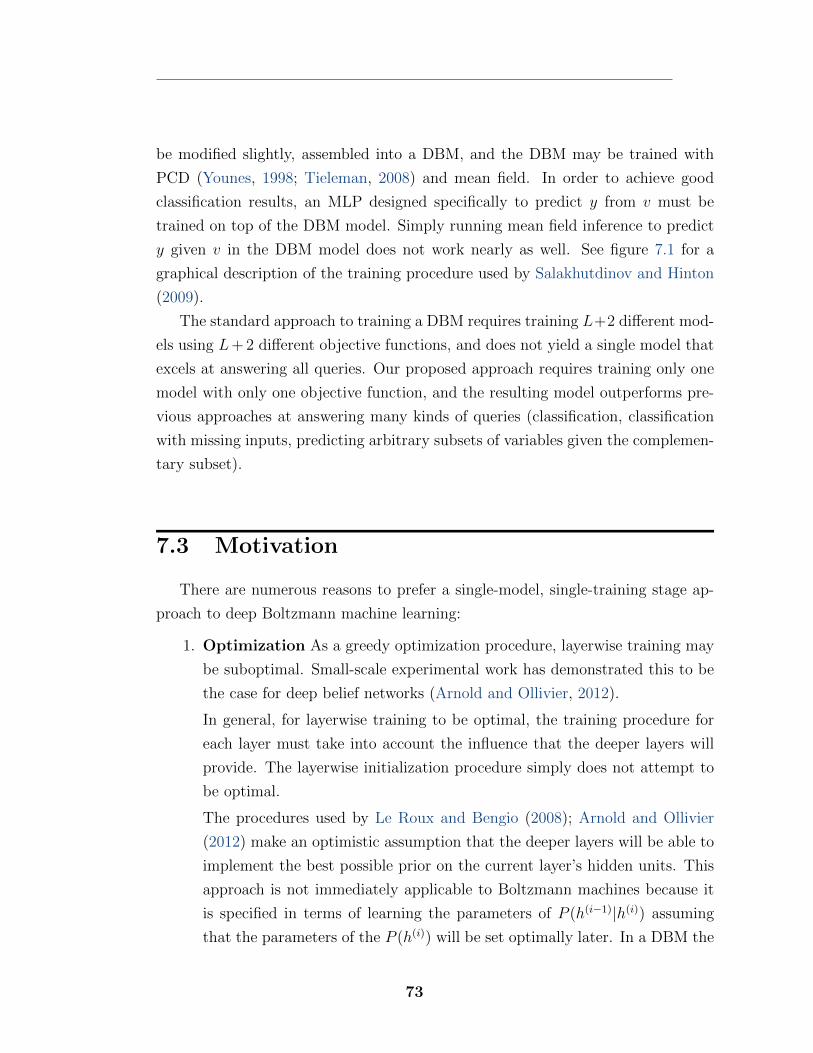
be modified slightly, assembled into a DBM, and the DBM may be trained with
PCD (Younes, 1998; Tieleman, 2008) and mean field. In order to achieve good
classification results, an MLP designed specifically to predict y from v must be
trained on top of the DBM model. Simply running mean field inference to predict
y given v in the DBM model does not work nearly as well. See figure 7.1 for a
graphical description of the training procedure used by Salakhutdinov and Hinton
(2009).
The standard approach to training a DBM requires training L+2 di↵erent mod-
els using L+2 di↵erent objective functions, and does not yield a single model that
excels at answering all queries. Our proposed approach requires training only one
model with only one objective function, and the resulting model outperforms pre-
vious approaches at answering many kinds of queries (classification, classification
with missing inputs, predicting arbitrary subsets of variables given the complemen-
tary subset).
7.3 Motivation
There are numerous reasons to prefer a single-model, single-training stage ap-
proach to deep Boltzmann machine learning:
1. Optimization As a greedy optimization procedure, layerwise training may
be suboptimal. Small-scale experimental work has demonstrated this to be
the case for deep belief networks (Arnold and Ollivier, 2012).
In general, for layerwise training to be optimal, the training procedure for
each layer must take into account the influence that the deeper layers will
provide. The layerwise initialization procedure simply does not attempt to
be optimal.
The procedures used by Le Roux and Bengio (2008); Arnold and Ollivier
(2012) make an optimistic assumption that the deeper layers will be able to
implement the best possible prior on the current layer’s hidden units. This
approach is not immediately applicable to Boltzmann machines because it
is specified in terms of learning the parameters of P (h(i�1)|h(i)) assuming
that the parameters of the P (h(i)) will be set optimally later. In a DBM the
73
symmetrical nature of the interactions between units means that these two
distributions share parameters, so it is not possible to set the parameters of
the one distribution, leave them fixed for the remainder of learning, and then
set the parameters of the other distribution. Moreover, model architectures
incorporating design features such as sparse connections, pooling, or factored
multilinear interactions make it di�cult to predict how best to structure one
layer’s hidden units in order for the next layer to make good use of them.
2. Probabilistic modeling Using multiple models and having some models
specialized for exactly one task (like predicting y from v) loses some of the
benefit of probabilistic modeling. If we have one model that excels at all
tasks, we can use inference in this model to answer arbitrary queries, perform
classification with missing inputs, and so on. The standard DBM training
procedure gives this up by training a rich probabilistic model and then using
it as just a feature extractor for an MLP.
3. Simplicity Needing to implement multiple models and training stages
makes the cost of developing software with DBMs greater, and makes using
them more cumbersome. Beyond the software engineering considerations,
it can be di�cult to monitor training and tell what kind of results during
layerwise RBM pretraining will correspond to good DBM classification ac-
curacy later. Our joint training procedure allows the user to monitor the
model’s ability of interest (usually ability to classify y given v) from the very
start of training.
7.4 Methods
We now described the new methods proposed in this paper, and some pre-
existing methods that we compare against.
7.4.1 Multi-prediction Training
Our proposed approach is to directly train the DBM to be good at solving
all possible variational inference problems. We call this multi-prediction training
74
because the procedure involves training the model to predict any subset of variables
given the complement of that subset of variables.
Let O be a vector containing all variables that are observed during training. For
a purely unsupervised learning task, O is just v itself. In the supervised setting,
O = [v, y]>. Note that y won’t be observed at test time, only training time. Let
D be the training set, i.e. a collection of values of O. Let S be a sequence of
subsets of the possible indices of O. Let Qi
be the variational (e.g., mean-field)
approximation to the joint of OSi and h given O�Si .
Qi
(OSi , h) = argmin
Q
DKL
(Q(OSi , h)kP (O
Si , h | O�Si)) .
In all of the experiments presented in this paper, Q is constrained to be factorial,
though one could design model families for which it makes sense to use richer struc-
ture in Q. Note that there is not an explicit formula for Q; Q must be computed
by an iterative optimization process. In order to accomplish this minimization, we
run the mean field fixed point equations to convergence. Because each fixed point
update uses the output of a previous fixed point update as input, this optimization
procedure can be viewed as a recurrent neural network. (To simplify implemen-
tation, we don’t explicitly test for convergence, but run the recurrent net for a
pre-specified number of iterations that is chosen to be high enough that the net
usually converges)
We train the MP-DBM by using minibatch stochastic gradient descent on the
multi-prediction (MP) objective function
J(D, ✓) = �X
O2D
X
i
log Qi
(OSi)
In other words, the criterion for a single example O is a sum of several terms,
with term i measuring the model’s ability to predict (through a variational approx-
imation) a subset of the variables in the training set, OSi , given the remainder of
the observed variables, O�Si .
During SGD training, we sample minibatches of values of O and Si
. Sampling
O just means drawing an example from the training set. Sampling an Si
uniformly
simply requires sampling one bit (1 with probability 0.5) for each variable, to
determine whether that variable should be an input to the inference procedure
or a prediction target. To compute the gradient, we simply backprop the error
75
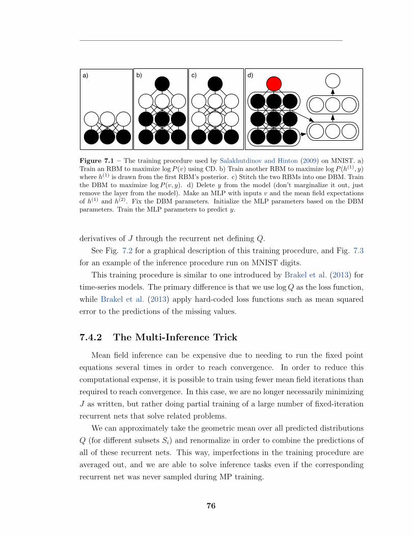
c) d)b)a)
Figure 7.1 – The training procedure used by Salakhutdinov and Hinton (2009) on MNIST. a)Train an RBM to maximize log P (v) using CD. b) Train another RBM to maximize log P (h(1), y)where h(1) is drawn from the first RBM’s posterior. c) Stitch the two RBMs into one DBM. Trainthe DBM to maximize log P (v, y). d) Delete y from the model (don’t marginalize it out, justremove the layer from the model). Make an MLP with inputs v and the mean field expectationsof h(1) and h(2). Fix the DBM parameters. Initialize the MLP parameters based on the DBMparameters. Train the MLP parameters to predict y.
derivatives of J through the recurrent net defining Q.
See Fig. 7.2 for a graphical description of this training procedure, and Fig. 7.3
for an example of the inference procedure run on MNIST digits.
This training procedure is similar to one introduced by Brakel et al. (2013) for
time-series models. The primary di↵erence is that we use log Q as the loss function,
while Brakel et al. (2013) apply hard-coded loss functions such as mean squared
error to the predictions of the missing values.
7.4.2 The Multi-Inference Trick
Mean field inference can be expensive due to needing to run the fixed point
equations several times in order to reach convergence. In order to reduce this
computational expense, it is possible to train using fewer mean field iterations than
required to reach convergence. In this case, we are no longer necessarily minimizing
J as written, but rather doing partial training of a large number of fixed-iteration
recurrent nets that solve related problems.
We can approximately take the geometric mean over all predicted distributions
Q (for di↵erent subsets Si
) and renormalize in order to combine the predictions of
all of these recurrent nets. This way, imperfections in the training procedure are
averaged out, and we are able to solve inference tasks even if the corresponding
recurrent net was never sampled during MP training.
76
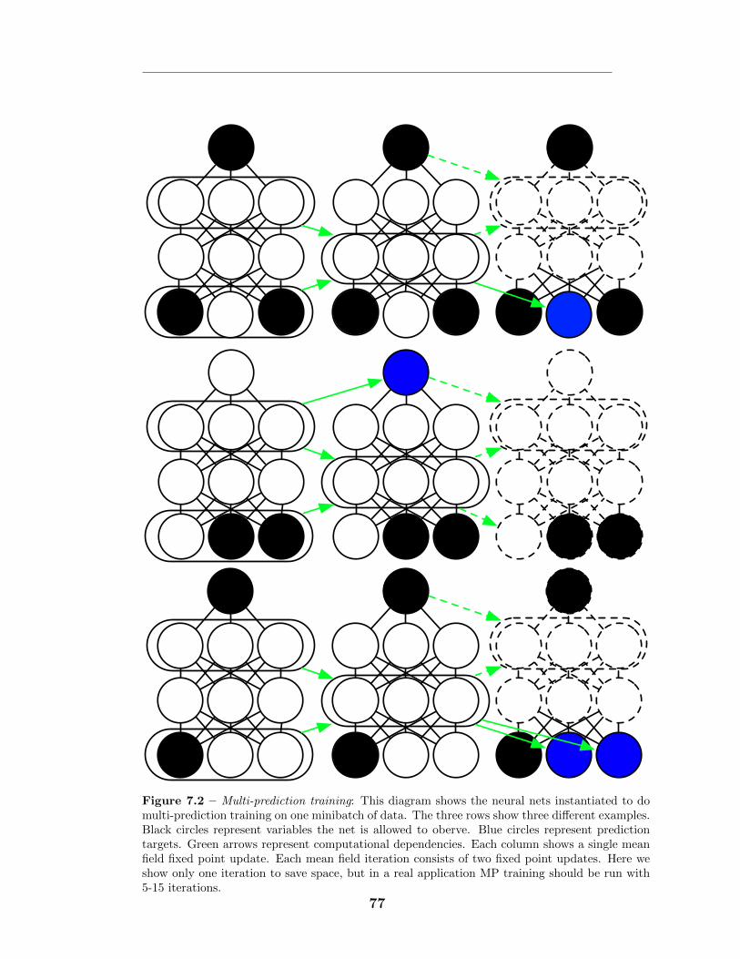
Figure 7.2 – Multi-prediction training: This diagram shows the neural nets instantiated to domulti-prediction training on one minibatch of data. The three rows show three di↵erent examples.Black circles represent variables the net is allowed to oberve. Blue circles represent predictiontargets. Green arrows represent computational dependencies. Each column shows a single meanfield fixed point update. Each mean field iteration consists of two fixed point updates. Here weshow only one iteration to save space, but in a real application MP training should be run with5-15 iterations.
77
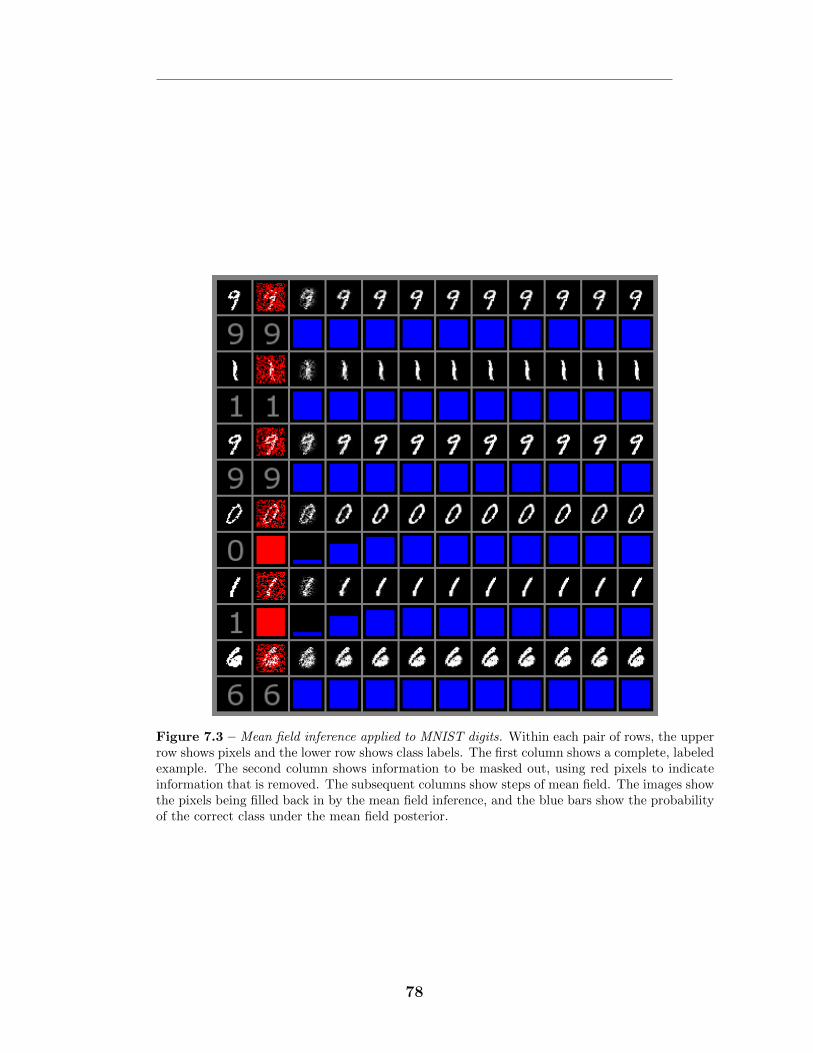
Figure 7.3 – Mean field inference applied to MNIST digits. Within each pair of rows, the upperrow shows pixels and the lower row shows class labels. The first column shows a complete, labeledexample. The second column shows information to be masked out, using red pixels to indicateinformation that is removed. The subsequent columns show steps of mean field. The images showthe pixels being filled back in by the mean field inference, and the blue bars show the probabilityof the correct class under the mean field posterior.
78
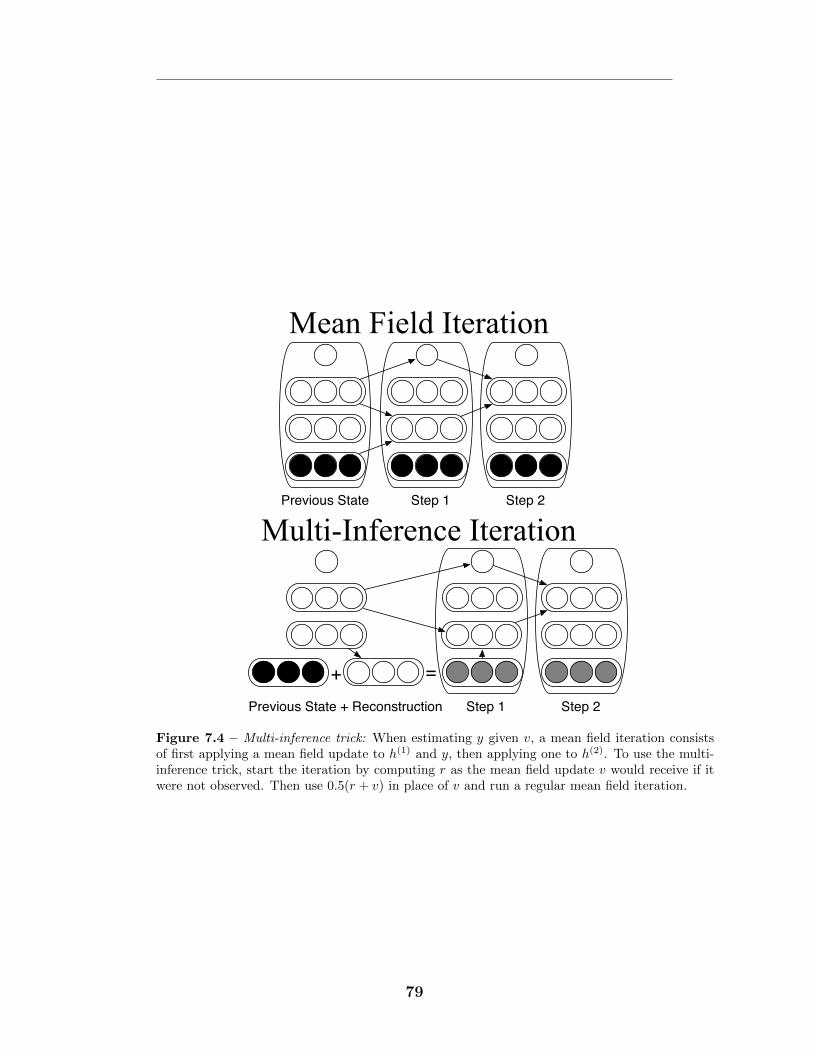
Mean Field Iteration
Multi-Inference Iteration
+ =
Step 1 Step 2Previous State + Reconstruction
Step 1 Step 2Previous State
Figure 7.4 – Multi-inference trick: When estimating y given v, a mean field iteration consistsof first applying a mean field update to h(1) and y, then applying one to h(2). To use the multi-inference trick, start the iteration by computing r as the mean field update v would receive if itwere not observed. Then use 0.5(r + v) in place of v and run a regular mean field iteration.
79
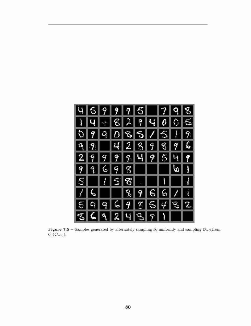
Figure 7.5 – Samples generated by alternately sampling Si uniformly and sampling O�Si fromQi(O�Si).
80
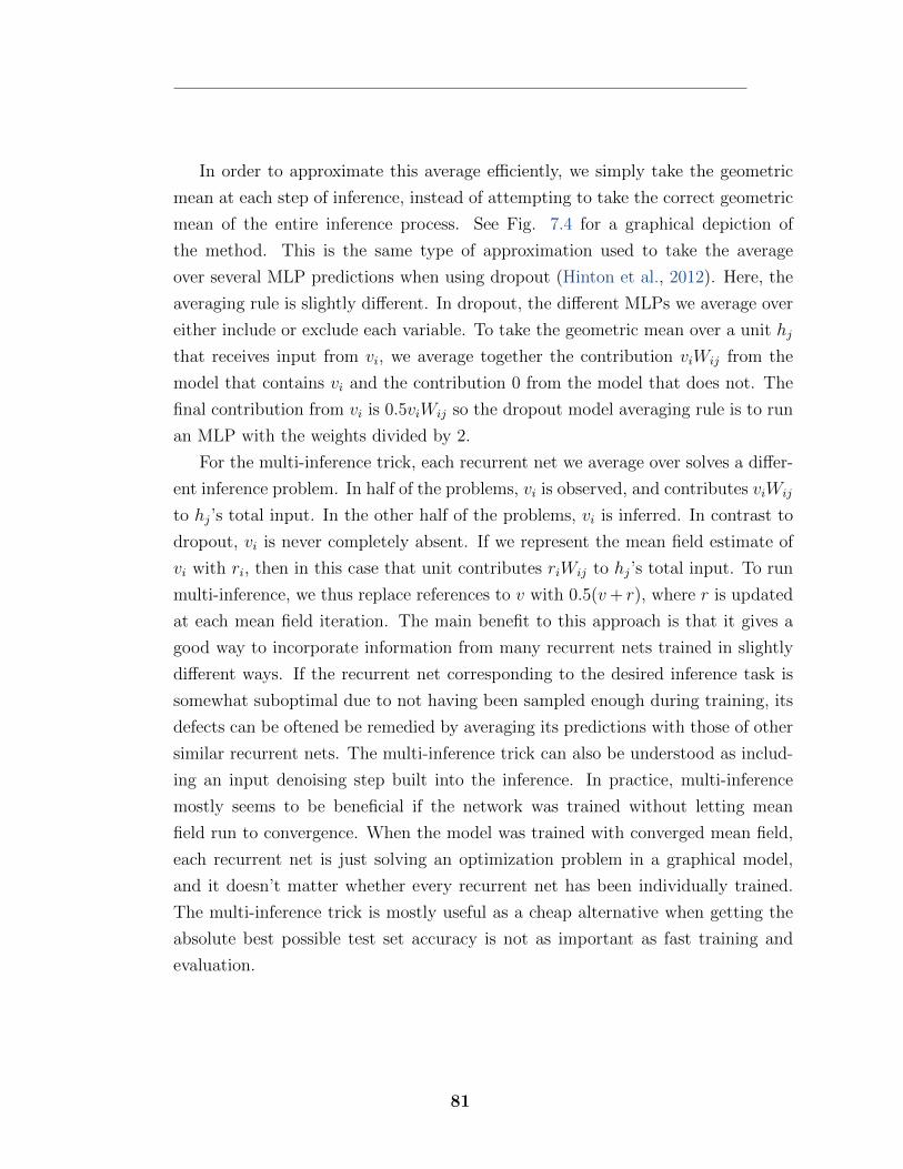
In order to approximate this average e�ciently, we simply take the geometric
mean at each step of inference, instead of attempting to take the correct geometric
mean of the entire inference process. See Fig. 7.4 for a graphical depiction of
the method. This is the same type of approximation used to take the average
over several MLP predictions when using dropout (Hinton et al., 2012). Here, the
averaging rule is slightly di↵erent. In dropout, the di↵erent MLPs we average over
either include or exclude each variable. To take the geometric mean over a unit hj
that receives input from vi
, we average together the contribution vi
Wij
from the
model that contains vi
and the contribution 0 from the model that does not. The
final contribution from vi
is 0.5vi
Wij
so the dropout model averaging rule is to run
an MLP with the weights divided by 2.
For the multi-inference trick, each recurrent net we average over solves a di↵er-
ent inference problem. In half of the problems, vi
is observed, and contributes vi
Wij
to hj
’s total input. In the other half of the problems, vi
is inferred. In contrast to
dropout, vi
is never completely absent. If we represent the mean field estimate of
vi
with ri
, then in this case that unit contributes ri
Wij
to hj
’s total input. To run
multi-inference, we thus replace references to v with 0.5(v + r), where r is updated
at each mean field iteration. The main benefit to this approach is that it gives a
good way to incorporate information from many recurrent nets trained in slightly
di↵erent ways. If the recurrent net corresponding to the desired inference task is
somewhat suboptimal due to not having been sampled enough during training, its
defects can be oftened be remedied by averaging its predictions with those of other
similar recurrent nets. The multi-inference trick can also be understood as includ-
ing an input denoising step built into the inference. In practice, multi-inference
mostly seems to be beneficial if the network was trained without letting mean
field run to convergence. When the model was trained with converged mean field,
each recurrent net is just solving an optimization problem in a graphical model,
and it doesn’t matter whether every recurrent net has been individually trained.
The multi-inference trick is mostly useful as a cheap alternative when getting the
absolute best possible test set accuracy is not as important as fast training and
evaluation.
81
7.4.3 Justification and advantages
In the case where we run the recurrent net for predicting Q to convergence, the
multi-prediction training algorithm follows the gradient of the objective function
J . This can be viewed as a mean field approximation to the generalized pseudo-
likelihood.
While both pseudolikelihood and likelihood are asymptotically consistent esti-
mators, their behavior in the limited data case is di↵erent. Maximum likelihood
should be better if the overall goal is to draw realistic samples from the model, but
generalized pseudolikelihood can often be better for training a model to answer
queries conditioning on sets similar to the Si
used during training.
Note that our variational approximation is not quite the same as the way vari-
ational approximations are usually applied. We use variational inference to ensure
that the distributions we shape using backprop are as close as possible to the
true conditionals. This is di↵erent from the usual approach to variational learn-
ing, where Q is used to define a lower bound on the log likelihood and variational
inference is used to make the bound as tight as possible.
In the case where the recurrent net is not trained to convergence, there is an
alternate way to justify MP training. Rather than doing variational learning on a
single probabilistic model, the MP procedure trains a family of recurrent nets to
solve related prediction problems by running for some fixed number of iterations.
Each recurrent net is trained only on a subset of the data (and most recurrent nets
are never trained at all, but only work because they share parameters with the
others). In this case, the multi-inference trick allows us to justify MP training as
approximately training an ensemble of recurrent nets using bagging.
Stoyanov et al. (2011) have observed that a training strategy similar to MPT
(but lacking the multi-inference trick) is useful because it trains the model to work
well with the inference approximations it will be evaluated with at test time. We
find these properties to be useful as well. The choice of this type of variational learn-
ing combined with the underlying generalized pseudolikelihood objective makes an
MP-DBM very well suited for solving approximate inference problems but not very
well suited for sampling.
Our primary design consideration when developing multi-prediction training
was ensuring that the learning rule was state-free. PCD training uses persistent
Markov chains to estimate the gradient. These Markov chains are used to approx-
82
imately sample from the model, and only sample from approximately the right
distribution if the model parameters evolve slowly. The MP training rule does not
make any reference to earlier training steps, and can be computed with no burn in.
This means that the accuracy of the MP gradient is not dependent on properties
of the training algorithm such as the learning rate which can easily break PCD for
many choices of the hyperparameters.
Another benefit of MP is that it is easy to obtain an unbiased estimate of the
MP objective from a small number of samples of v and i. This is in contrast
to the log likelihood, which requires estimating the log partition function. The
best known method for doing so is AIS, which is relatively expensive (Neal, 2001).
Cheap estimates of the objective function enable early stopping based on the MP-
objective (though we generally use early stopping based on classification accuracy)
and optimization based on line searches (though we do not explore that possibility
in this paper).
7.4.4 Regularization
In order to obtain good generalization performance, Salakhutdinov and Hinton
(2009) regularized both the weights and the activations of the network.
Salakhutdinov and Hinton (2009) regularize the weights using an L2 penalty. We
find that for joint training, it is critically important to not do this (on the MNIST
dataset, we were not able to find any MP-DBM hyperparameter configuration
involving weight decay that performs as well as layerwise DBMs, but without weight
decay MP-DBMs outperform DBMs). When the second layer weights are not
trained well enough for them to be useful for modeling the data, the weight decay
term will drive them to become very small, and they will never have an opportunity
to recover. It is much better to use constraints on the norms of the columns of the
weight vectors as done by Srebro and Shraibman (2005).
Salakhutdinov and Hinton (2009) regularize the activities of the hidden units
with a somewhat complicated sparsity penalty. See
http://www.mit.edu/~rsalakhu/DBM.html for details. We use max(|Eh⇠Q(h)
[h]�t| � �, 0) and backpropagate this through the entire inference graph. t and � are
hyperparameters.
83
7.4.5 Related work: centering
Montavon and Muller (2012) showed that an alternative, “centered” representa-
tion of the DBM results in successful generative training without a greedy layerwise
pretraining step. However, centered DBMs have never been shown to have good
classification performance. We therefore evaluate the classification performance of
centering in this work. We consider two methods of variational PCD training. In
one, we use Rao-Blackwellization (Blackwell, 1947; Kolmogorov, 1953; Rao, 1973)
of the negative phase particles to reduce the variance of the negative phase. In the
other variant (“centering+”), we use a special negative phase that Salakhutdinov
and Hinton (2009) found useful. This negative phase uses a small amount of mean
field, which reduces the variance further but introduces some bias, and has better
symmetry with the positive phase. See http://www.mit.edu/~rsalakhu/DBM.html
for details.
7.4.6 Sampling, and a connection to GSNs
The focus of this paper is solving inference problems, not generating samples, so
we do not investigate the sampling properties of MP-DBMs extensively. However, it
is interesting to note that an MP-DBM can be viewed as a collection of dependency
networks (Heckerman et al., 2000) with shared parameters. Dependency networks
are a special case of generative stochastic networks or GSNs (Bengio et al. (2014),
section 3.4). This means that the MP-DBM is associated with a distribution arising
out of the Markov chain in which at each step one samples an Si
uniformly and then
samples O from Qi
(O). Example samples are shown in figure 7.5. Furthermore, it
means that if MPT is a consistent estimator of the conditional distributions, then
MPT is a consistent estimator of the probability distribution defined by the sta-
tionary distribution of this Markov chain. Samples drawn by Gibbs sampling in the
DBM model do not look as good (probably because the variational approximation
is too damaging). This suggests that the perspective of the MP-DBM as a GSN
merits further investigation.
84
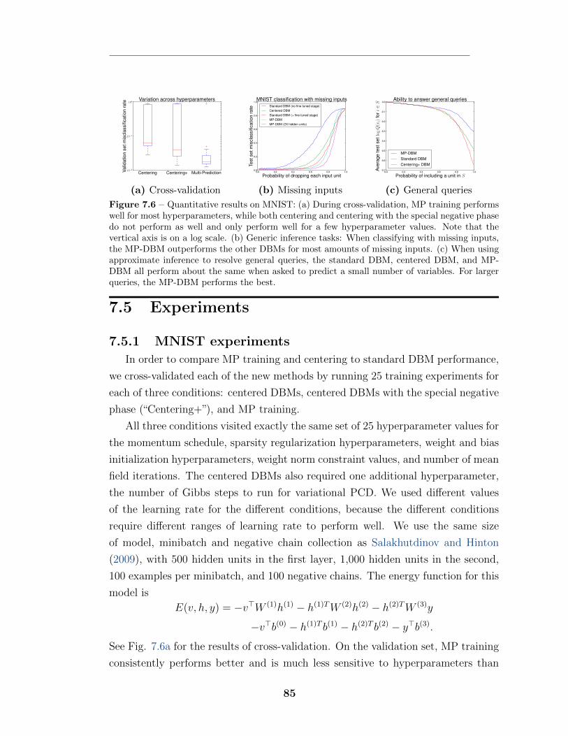
Centering Centering+ Multi-Prediction10�2
10�1
100
Valid
atio
nse
tmis
clas
sific
atio
nra
te Variation across hyperparameters
(a) Cross-validation
0.0 0.2 0.4 0.6 0.8 1.0
Probability of dropping each input unit0.0
0.2
0.4
0.6
0.8
1.0
Test
setm
iscl
assi
ficat
ion
rate
MNIST classification with missing inputsStandard DBM (no fine tuned stage)Centered DBMStandard DBM (+ fine tuned stage)MP-DBMMP-DBM (2X hidden units)
(b) Missing inputs
0.0 0.2 0.4 0.6 0.8 1.0
Probability of including a unit in S-0.7
-0.6
-0.5
-0.4
-0.3
-0.2
-0.1
0.0
Aver
age
test
setl
ogQ
(vi)
fori
2S
Ability to answer general queries
MP-DBMStandard DBMCentering+ DBM
(c) General queries
Figure 7.6 – Quantitative results on MNIST: (a) During cross-validation, MP training performswell for most hyperparameters, while both centering and centering with the special negative phasedo not perform as well and only perform well for a few hyperparameter values. Note that thevertical axis is on a log scale. (b) Generic inference tasks: When classifying with missing inputs,the MP-DBM outperforms the other DBMs for most amounts of missing inputs. (c) When usingapproximate inference to resolve general queries, the standard DBM, centered DBM, and MP-DBM all perform about the same when asked to predict a small number of variables. For largerqueries, the MP-DBM performs the best.
7.5 Experiments
7.5.1 MNIST experimentsIn order to compare MP training and centering to standard DBM performance,
we cross-validated each of the new methods by running 25 training experiments for
each of three conditions: centered DBMs, centered DBMs with the special negative
phase (“Centering+”), and MP training.
All three conditions visited exactly the same set of 25 hyperparameter values for
the momentum schedule, sparsity regularization hyperparameters, weight and bias
initialization hyperparameters, weight norm constraint values, and number of mean
field iterations. The centered DBMs also required one additional hyperparameter,
the number of Gibbs steps to run for variational PCD. We used di↵erent values
of the learning rate for the di↵erent conditions, because the di↵erent conditions
require di↵erent ranges of learning rate to perform well. We use the same size
of model, minibatch and negative chain collection as Salakhutdinov and Hinton
(2009), with 500 hidden units in the first layer, 1,000 hidden units in the second,
100 examples per minibatch, and 100 negative chains. The energy function for this
model is
E(v, h, y) = �v>W (1)h(1) � h(1)T W (2)h(2) � h(2)T W (3)y
�v>b(0) � h(1)T b(1) � h(2)T b(2) � y>b(3).
See Fig. 7.6a for the results of cross-validation. On the validation set, MP training
consistently performs better and is much less sensitive to hyperparameters than
85
the other methods. This is likely because the state-free nature of the learning rule
makes it perform better with settings of the learning rate and momentum schedule
that result in the model distribution changing too fast for a method based on
Markov chains to keep up.
When we add an MLP classifier (as shown in Fig. 7.1d), the best “Center-
ing+” DBM obtains a classification error of 1.22% on the test set. The best MP-
DBM obtains a classification error of 0.88%. This compares to 0.95% obtained by
Salakhutdinov and Hinton (2009).
If instead of adding an MLP to the model, we simply train a larger MP-DBM
with twice as many hidden units in each layer, and apply the multi-inference trick,
we obtain a classification error rate of 0.91%. In other words, we are able to classify
nearly as well using a single large DBM and a generic inference procedure, rather
than using a DBM followed by an entirely separate MLP model specialized for
classification.
The original DBM was motivated primarily as a generative model with a high
AIS score and as a means of initializing a classifier. Here we explore some more
uses of the DBM as a generative model. Fig. 7.6b shows an evaluation of various
DBM’s ability to classify with missing inputs. Fig. 7.6c shows an evaluation of
their ability to resolve queries about random subsets of variables. In both cases we
find that the MP-DBM performs the best for most amounts of missing inputs.
7.5.2 NORB experiments
NORB consists of 96⇥96 binocular greyscale images of objects from five di↵erent
categories, under a variety of pose and lighting conditions. Salakhutdinov and
Hinton (2009) preprocessed the images by resampling them with bigger pixels near
the border of the image, yielding an input vector of size 8,976. We used this
preprocessing as well. Salakhutdinov and Hinton (2009) then trained an RBM
with 4,000 binary hidden units and Gaussian visible units to preprocess the data
into an all-binary representation, and trained a DBM with two hidden layers of
4,000 units each on this representation. Since the goal of this work is to provide a
single unified model and training algorithm, we do not train a separate Gaussian
RBM. Instead we train a single MP-DBM with Gaussian visible units and three
hidden layers of 4,000 units each. The energy function for this model is
86
E(v, h, y) = �(v � µ)>�W (1)h(1) � h(1)T W (2)h(2) � h(2)T W (3)h(3) � h(3)T W (4)y
+1
2(v � µ)>�(v � µ) � h(1)T b(1) � h(2)T b(2) � h(3)T b(3) � y>b(4).
where µ is a learned vector of visible unit means and � is a learned diagonalprecision matrix.
By adding an MLP on top of the MP-DBM, following the same architecture as
Salakhutdinov and Hinton (2009), we were able to obtain a test set error of 10.6%.
This is a slight improvement over the standard DBM’s 10.8%.
On MNIST we were able to outperform the DBM without using the MLP clas-
sifier because we were able to train a larger MP-DBM. On NORB, the model size
used by Salakhutdinov and Hinton (2009) is already as large as we are able to fit
on most of our graphics cards, so we were not able to do the same for this dataset.
It is possible to do better on NORB using convolution or synthetic transformations
of the training data. We did not evaluate the e↵ect of these techniques on the
MP-DBM because our present goal is not to obtain state-of-the-art object recog-
nition performance but only to verify that our joint training procedure works as
well as the layerwise training procedure for DBMs. There is no public demo code
available for the standard DBM on this dataset, and we were not able to reproduce
the standard DBM results (layerwise DBM training requires significant experience
and intuition). We therefore can’t compare the MP-DBM to the original DBM
in terms of answering general queries or classification with missing inputs on this
dataset.
7.6 Conclusion
This paper has demonstrated that MP training and the multi-inference trick
provide a means of training a single model, with a single stage of training, that
matches the performance of standard DBMs but still works as a general proba-
bilistic model, capable of handling missing inputs and answering general queries.
We have verified that MP training outperforms the standard training procedure at
classification on the MNIST and NORB datasets where the original DBM was first
applied. We have shown that MP training works well with binary, Gaussian, and
softmax units, as well as architectures with either two or three hidden layers. In
87

future work, we hope to apply the MP-DBM to more practical applications, and
explore techniques, such as dropout, that could improve its performance further.
Acknowledgments
We would like to thank the developers of Theano (Bergstra et al., 2010; Bastien
et al., 2012), Pylearn2 (Goodfellow et al., 2013). We would also like to thank
NSERC, Compute Canada, and Calcul Quebec for providing computational re-
sources.
88
8 Prologue to Third Article
8.1 Article Details
Maxout Networks. Ian J. Goodfellow, David Warde-Farley, Mehdi Mirza,
Aaron Courville, and Yoshua Bengio. Proceedings of the 30th International Con-
ference on Machine Learning (ICML ’13), pp. 1319-1327.
Personal Contribution. The idea for the maxout activation function and using
it in combination with dropout was my own. All of my co-authors suggested experi-
ments for understanding the e↵ectiveness of this combination. David Warde-Farley,
Mehdi Mirza, and I jointly ran these more scientific experiments. I wrote the code
for the activation function itself. David Warde-Farley and I jointly wrote the code
to accelerate convolution in Theano along with help from other Theano developers.
I found the best hyperparameters for both versions of the MNIST dataset. I found
hyperparameters for non-augmented CIFAR-10 that improved upon the state of
the art, and then David Warde-Farley improved upon mine further and obtained
the state of the art on augmented CIFAR-10 as well. I found the best hyperparam-
eters for CIFAR-100. Mehdi Mirza implemented the infrastructure code needed
to handle large datasets in order to work with SVHN. He also implemented the
preprocessing code for SVHN and found the best hyperparameters for this dataset.
David Warde-Farley, Mehdi Mirza, and I each made figures for the paper. All
authors contributed to the writing of the paper. I supplied the basic idea for the
universal approximation proof, and Aaron Courville wrote the formal proof sketch.
8.2 Context
At the time that we wrote this article, the dropout (Hinton et al., 2012) algo-
rithm had been recently introduced. In the excitement following the introduction
89
of dropout, we were interested in finding a model family that would synergize
well with dropout. Dropout also presented the opportunity to train models that
had previously su↵ered from overfitting. The maxout activation function, with its
cross-channel pooling, is one such model.
8.3 Contributions
The main contribution of this paper is to introduce a new activation function
for feedforward neural networks that significantly improves their performance. We
also perform detailed experiments to explain these performance gains.
8.4 Recent Developments
Since its publication, this work has been frequently cited and expanded upon.
Wang and Manning (2013) developed a fast analytical approximation to dropout
and included formulas for using their method with maxout layers. Smirnov (2013)
used maxout for whale call detection. Xie et al. (2013) used maxout to rank highly
in a machine learning contest (Goodfellow et al., 2013). Miao et al. (2013) used
maxout for low resource speech recognition. Cai et al. (2013) also applied maxout
to speech recognition, and found that maxout works well even without dropout
training, so long as the dataset is large and the number of pieces per maxout unit
is low. Alsharif and Pineau (2013) used maxout networks to implement the condi-
tional probability distributions in a larger graphical model used to transcribe text
from photos. Goodfellow et al. (2014) used maxout networks directly to transcribe
house numbers from photos, as presented in chapter 11.
90
9Maxout Networks
9.1 Introduction
Dropout (Hinton et al., 2012) provides an inexpensive and simple means of
both training a large ensemble of models that share parameters and approximately
averaging together these models’ predictions. Dropout applied to multilayer per-
ceptrons and deep convolutional networks has improved the state of the art on
tasks ranging from audio classification to very large scale object recognition (Hin-
ton et al., 2012; Krizhevsky et al., 2012). While dropout is known to work well in
practice, it has not previously been demonstrated to actually perform model aver-
aging for deep architectures 1 . Dropout is generally viewed as an indiscriminately
applicable tool that reliably yields a modest improvement in performance when
applied to almost any model.
We argue that rather than using dropout as a slight performance enhancement
applied to arbitrary models, the best performance may be obtained by directly de-
signing a model that enhances dropout’s abilities as a model averaging technique.
Training using dropout di↵ers significantly from previous approaches such as ordi-
nary stochastic gradient descent. Dropout is most e↵ective when taking relatively
large steps in parameter space. In this regime, each update can be seen as mak-
ing a significant update to a di↵erent model on a di↵erent subset of the training
set. The ideal operating regime for dropout is when the overall training procedure
resembles training an ensemble with bagging under parameter sharing constraints.
This di↵ers radically from the ideal stochastic gradient operating regime in which a
single model makes steady progress via small steps. Another consideration is that
dropout model averaging is only an approximation when applied to deep models.
Explicitly designing models to minimize this approximation error may thus enhance
dropout’s performance as well.
1. Between submission and publication of this paper, we have learned that Srivastava (2013)performed experiments on this subject similar to ours.
91
We propose a simple model that we call maxout that has beneficial characteris-
tics both for optimization and model averaging with dropout. We use this model in
conjunction with dropout to set the state of the art on four benchmark datasets 2 .
9.2 Review of dropout
Dropout is a technique that can be applied to deterministic feedforward archi-
tectures that predict an output y given input vector v. These architectures contain
a series of hidden layers h = {h(1), . . . , h(L)}. Dropout trains an ensemble of models
consisting of the set of all models that contain a subset of the variables in both v
and h. The same set of parameters ✓ is used to parameterize a family of distri-
butions p(y | v; ✓, µ) where µ 2 M is a binary mask determining which variables
to include in the model. On each presentation of a training example, we train
a di↵erent sub-model by following the gradient of log p(y | v; ✓, µ) for a di↵erent
randomly sampled µ. For many parameterizations of p (such as most multilayer
perceptrons) the instantiation of di↵erent sub-models p(y | v; ✓, µ) can be obtained
by elementwise multiplication of v and h with the mask µ. Dropout training is
similar to bagging (Breiman, 1994), where many di↵erent models are trained on
di↵erent subsets of the data. Dropout training di↵ers from bagging in that each
model is trained for only one step and all of the models share parameters. For
this training procedure to behave as if it is training an ensemble rather than a
single model, each update must have a large e↵ect, so that it makes the sub-model
induced by that µ fit the current input v well.
The functional form becomes important when it comes time for the ensem-
ble to make a prediction by averaging together all the sub-models’ predictions.
Most prior work on bagging averages with the arithmetic mean, but it is not
obvious how to do so with the exponentially many models trained by dropout.
Fortunately, some model families yield an inexpensive geometric mean. When
p(y | v; ✓) = softmax(v>W +b), the predictive distribution defined by renormalizing
the geometric mean of p(y | v; ✓, µ) over M is simply given by softmax(v>W/2+b).
In other words, the average prediction of exponentially many sub-models can be
2. Code and hyperparameters available at http://www-etud.iro.umontreal.ca/~goodfeli/maxout.html
92
computed simply by running the full model with the weights divided by 2. This
result holds exactly in the case of a single layer softmax model. Previous work on
dropout applies the same scheme in deeper architectures, such as multilayer per-
ceptrons, where the W/2 method is only an approximation to the geometric mean.
The approximation has not been characterized mathematically, but performs well
in practice.
9.3 Description of maxout
The maxout model is simply a feed-forward achitecture, such as a multilayer
perceptron or deep convolutional neural network, that uses a new type of activation
function: the maxout unit. Given an input x 2 Rd (x may be v, or may be a hidden
layer’s state), a maxout hidden layer implements the function
hi
(x) = maxj2[1,k]
zij
where zij
= x>W···ij + bij
, and W 2 Rd⇥m⇥k and b 2 Rm⇥k are learned parameters.
In a convolutional network, a maxout feature map can be constructed by taking the
maximum across k a�ne feature maps (i.e., pool across channels, in addition spatial
locations). When training with dropout, we perform the elementwise multiplication
with the dropout mask immediately prior to the multiplication by the weights in
all cases–we do not drop inputs to the max operator. A single maxout unit can
be interpreted as making a piecewise linear approximation to an arbitrary convex
function. Maxout networks learn not just the relationship between hidden units,
but also the activation function of each hidden unit. See Fig. 9.1 for a graphical
depiction of how this works.
Maxout abandons many of the mainstays of traditional activation function de-
sign. The representation it produces is not sparse at all (see Fig. 9.2), though
the gradient is highly sparse and dropout will artificially sparsify the e↵ective rep-
resentation during training. While maxout may learn to saturate on one side or
the other this is a measure zero event (so it is almost never bounded from above).
While a significant proportion of parameter space corresponds to the function being
bounded from below, maxout is not constrained to learn to be bounded at all. Max-
out is locally linear almost everywhere, while many popular activation functions
93
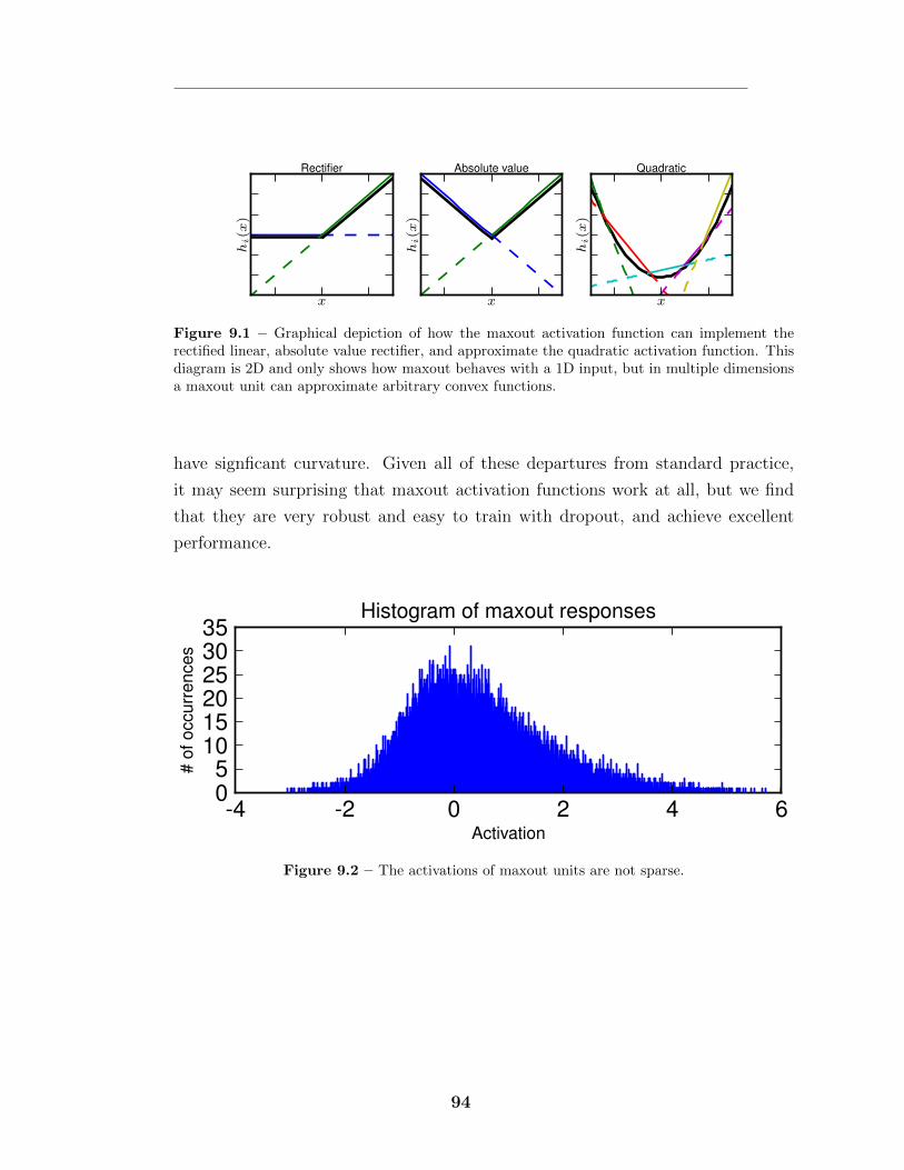
x
hi(x
)
Rectifier
x
hi(x
)
Absolute value
x
hi(x
)
Quadratic
Figure 9.1 – Graphical depiction of how the maxout activation function can implement therectified linear, absolute value rectifier, and approximate the quadratic activation function. Thisdiagram is 2D and only shows how maxout behaves with a 1D input, but in multiple dimensionsa maxout unit can approximate arbitrary convex functions.
have signficant curvature. Given all of these departures from standard practice,
it may seem surprising that maxout activation functions work at all, but we find
that they are very robust and easy to train with dropout, and achieve excellent
performance.
-4 -2 0 2 4 6Activation
05
101520253035
#of
occu
rren
ces
Histogram of maxout responses
Figure 9.2 – The activations of maxout units are not sparse.
94
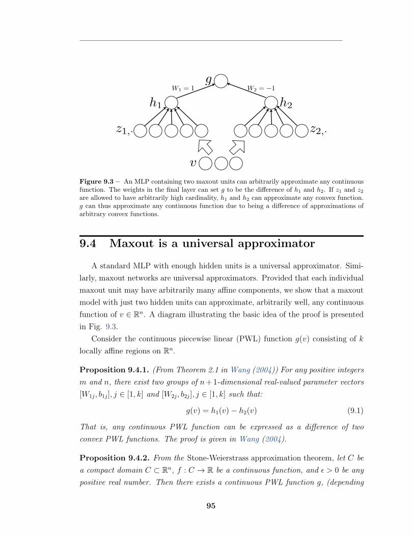
h2h1
g
z2,·z1,·
v
W1 = 1 W2 = �1
Figure 9.3 – An MLP containing two maxout units can arbitrarily approximate any continuousfunction. The weights in the final layer can set g to be the di↵erence of h1 and h2. If z1 and z2
are allowed to have arbitrarily high cardinality, h1 and h2 can approximate any convex function.g can thus approximate any continuous function due to being a di↵erence of approximations ofarbitrary convex functions.
9.4 Maxout is a universal approximator
A standard MLP with enough hidden units is a universal approximator. Simi-
larly, maxout networks are universal approximators. Provided that each individual
maxout unit may have arbitrarily many a�ne components, we show that a maxout
model with just two hidden units can approximate, arbitrarily well, any continuous
function of v 2 Rn. A diagram illustrating the basic idea of the proof is presented
in Fig. 9.3.
Consider the continuous piecewise linear (PWL) function g(v) consisting of k
locally a�ne regions on Rn.
Proposition 9.4.1. (From Theorem 2.1 in Wang (2004)) For any positive integers
m and n, there exist two groups of n+1-dimensional real-valued parameter vectors
[W1j
, b1j
], j 2 [1, k] and [W2j
, b2j
], j 2 [1, k] such that:
g(v) = h1
(v) � h2
(v) (9.1)
That is, any continuous PWL function can be expressed as a di↵erence of two
convex PWL functions. The proof is given in Wang (2004).
Proposition 9.4.2. From the Stone-Weierstrass approximation theorem, let C be
a compact domain C ⇢ Rn, f : C ! R be a continuous function, and ✏ > 0 be any
positive real number. Then there exists a continuous PWL function g, (depending
95
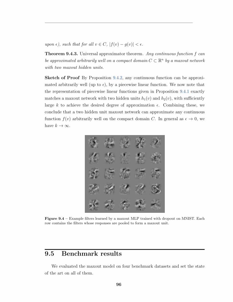
upon ✏), such that for all v 2 C, |f(v) � g(v)| < ✏.
Theorem 9.4.3. Universal approximator theorem. Any continuous function f can
be approximated arbitrarily well on a compact domain C ⇢ Rn by a maxout network
with two maxout hidden units.
Sketch of Proof By Proposition 9.4.2, any continuous function can be approxi-
mated arbitrarily well (up to ✏), by a piecewise linear function. We now note that
the representation of piecewise linear functions given in Proposition 9.4.1 exactly
matches a maxout network with two hidden units h1
(v) and h2
(v), with su�ciently
large k to achieve the desired degree of approximation ✏. Combining these, we
conclude that a two hidden unit maxout network can approximate any continuous
function f(v) arbitrarily well on the compact domain C. In general as ✏ ! 0, we
have k ! 1.
Figure 9.4 – Example filters learned by a maxout MLP trained with dropout on MNIST. Eachrow contains the filters whose responses are pooled to form a maxout unit.
9.5 Benchmark results
We evaluated the maxout model on four benchmark datasets and set the state
of the art on all of them.
96
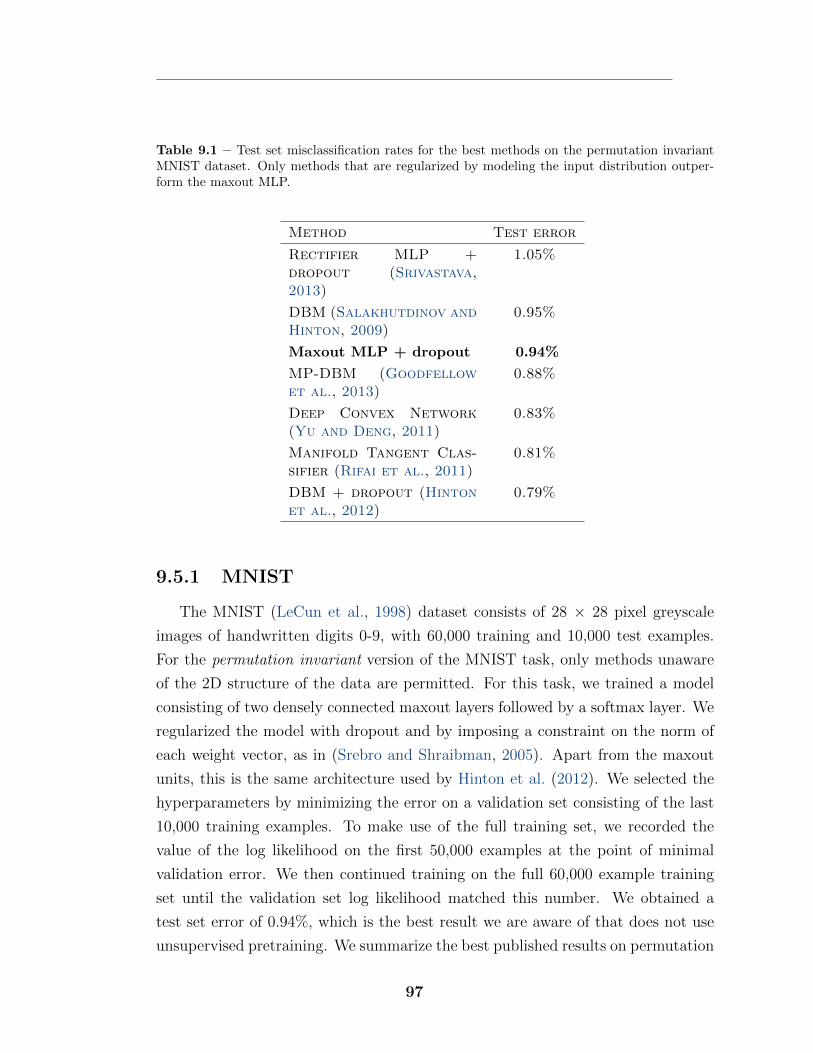
Table 9.1 – Test set misclassification rates for the best methods on the permutation invariantMNIST dataset. Only methods that are regularized by modeling the input distribution outper-form the maxout MLP.
Method Test error
Rectifier MLP +dropout (Srivastava,2013)
1.05%
DBM (Salakhutdinov andHinton, 2009)
0.95%
Maxout MLP + dropout 0.94%
MP-DBM (Goodfellowet al., 2013)
0.88%
Deep Convex Network(Yu and Deng, 2011)
0.83%
Manifold Tangent Clas-sifier (Rifai et al., 2011)
0.81%
DBM + dropout (Hintonet al., 2012)
0.79%
9.5.1 MNIST
The MNIST (LeCun et al., 1998) dataset consists of 28 ⇥ 28 pixel greyscale
images of handwritten digits 0-9, with 60,000 training and 10,000 test examples.
For the permutation invariant version of the MNIST task, only methods unaware
of the 2D structure of the data are permitted. For this task, we trained a model
consisting of two densely connected maxout layers followed by a softmax layer. We
regularized the model with dropout and by imposing a constraint on the norm of
each weight vector, as in (Srebro and Shraibman, 2005). Apart from the maxout
units, this is the same architecture used by Hinton et al. (2012). We selected the
hyperparameters by minimizing the error on a validation set consisting of the last
10,000 training examples. To make use of the full training set, we recorded the
value of the log likelihood on the first 50,000 examples at the point of minimal
validation error. We then continued training on the full 60,000 example training
set until the validation set log likelihood matched this number. We obtained a
test set error of 0.94%, which is the best result we are aware of that does not use
unsupervised pretraining. We summarize the best published results on permutation
97
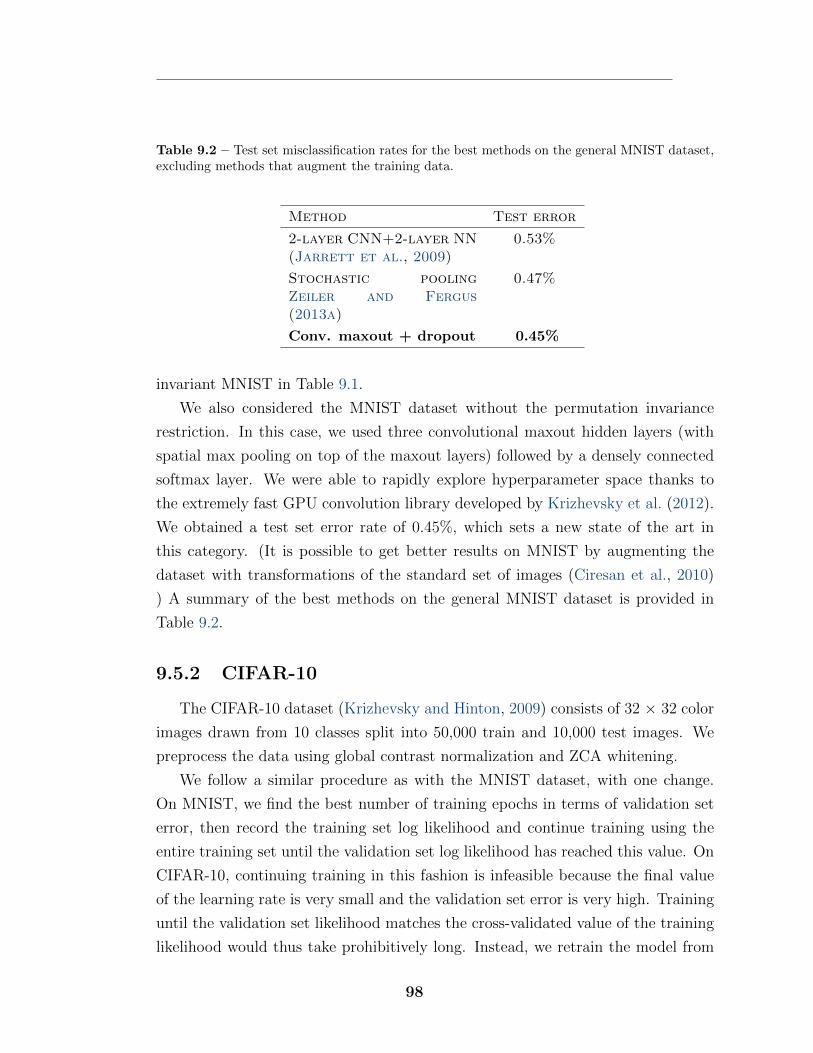
Table 9.2 – Test set misclassification rates for the best methods on the general MNIST dataset,excluding methods that augment the training data.
Method Test error
2-layer CNN+2-layer NN(Jarrett et al., 2009)
0.53%
Stochastic poolingZeiler and Fergus(2013a)
0.47%
Conv. maxout + dropout 0.45%
invariant MNIST in Table 9.1.
We also considered the MNIST dataset without the permutation invariance
restriction. In this case, we used three convolutional maxout hidden layers (with
spatial max pooling on top of the maxout layers) followed by a densely connected
softmax layer. We were able to rapidly explore hyperparameter space thanks to
the extremely fast GPU convolution library developed by Krizhevsky et al. (2012).
We obtained a test set error rate of 0.45%, which sets a new state of the art in
this category. (It is possible to get better results on MNIST by augmenting the
dataset with transformations of the standard set of images (Ciresan et al., 2010)
) A summary of the best methods on the general MNIST dataset is provided in
Table 9.2.
9.5.2 CIFAR-10
The CIFAR-10 dataset (Krizhevsky and Hinton, 2009) consists of 32 ⇥ 32 color
images drawn from 10 classes split into 50,000 train and 10,000 test images. We
preprocess the data using global contrast normalization and ZCA whitening.
We follow a similar procedure as with the MNIST dataset, with one change.
On MNIST, we find the best number of training epochs in terms of validation set
error, then record the training set log likelihood and continue training using the
entire training set until the validation set log likelihood has reached this value. On
CIFAR-10, continuing training in this fashion is infeasible because the final value
of the learning rate is very small and the validation set error is very high. Training
until the validation set likelihood matches the cross-validated value of the training
likelihood would thus take prohibitively long. Instead, we retrain the model from
98
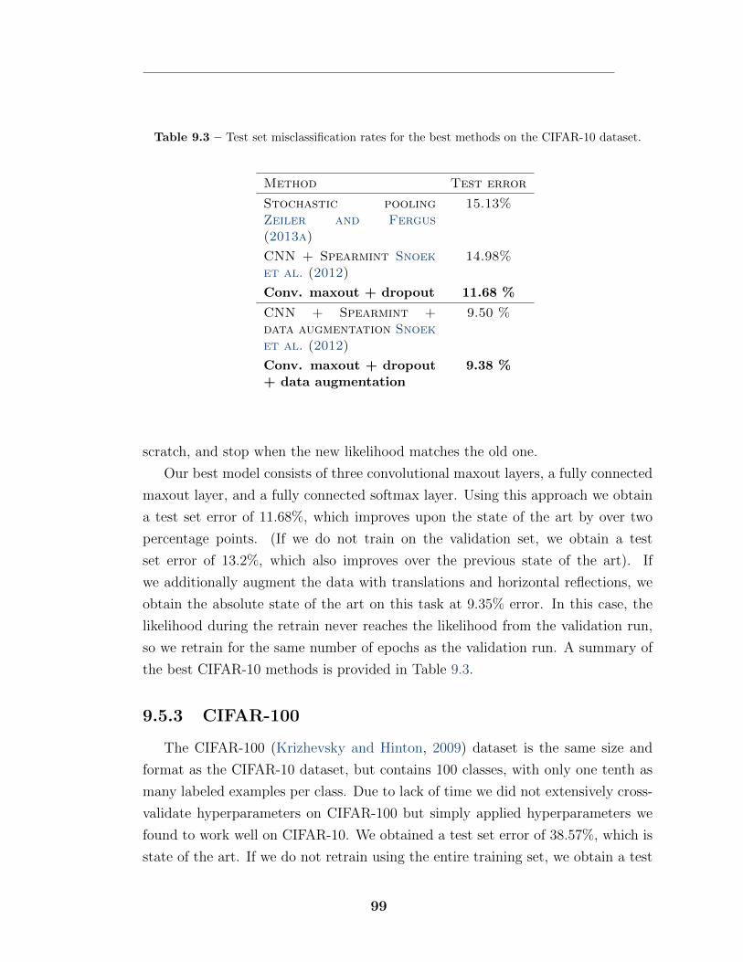
Table 9.3 – Test set misclassification rates for the best methods on the CIFAR-10 dataset.
Method Test error
Stochastic poolingZeiler and Fergus(2013a)
15.13%
CNN + Spearmint Snoeket al. (2012)
14.98%
Conv. maxout + dropout 11.68 %
CNN + Spearmint +data augmentation Snoeket al. (2012)
9.50 %
Conv. maxout + dropout+ data augmentation
9.38 %
scratch, and stop when the new likelihood matches the old one.
Our best model consists of three convolutional maxout layers, a fully connected
maxout layer, and a fully connected softmax layer. Using this approach we obtain
a test set error of 11.68%, which improves upon the state of the art by over two
percentage points. (If we do not train on the validation set, we obtain a test
set error of 13.2%, which also improves over the previous state of the art). If
we additionally augment the data with translations and horizontal reflections, we
obtain the absolute state of the art on this task at 9.35% error. In this case, the
likelihood during the retrain never reaches the likelihood from the validation run,
so we retrain for the same number of epochs as the validation run. A summary of
the best CIFAR-10 methods is provided in Table 9.3.
9.5.3 CIFAR-100
The CIFAR-100 (Krizhevsky and Hinton, 2009) dataset is the same size and
format as the CIFAR-10 dataset, but contains 100 classes, with only one tenth as
many labeled examples per class. Due to lack of time we did not extensively cross-
validate hyperparameters on CIFAR-100 but simply applied hyperparameters we
found to work well on CIFAR-10. We obtained a test set error of 38.57%, which is
state of the art. If we do not retrain using the entire training set, we obtain a test
99
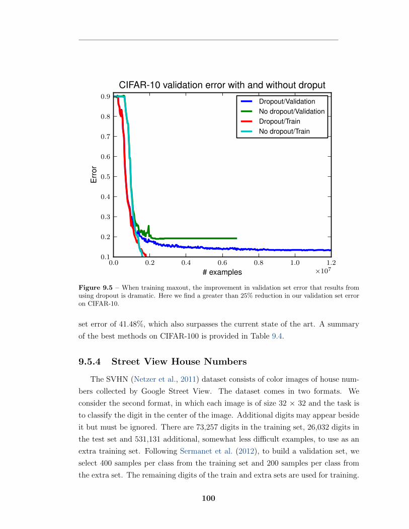
0.0 0.2 0.4 0.6 0.8 1.0 1.2
# examples ⇥10
7
0.1
0.2
0.3
0.4
0.5
0.6
0.7
0.8
0.9
Err
orCIFAR-10 validation error with and without droput
Dropout/ValidationNo dropout/ValidationDropout/TrainNo dropout/Train
Figure 9.5 – When training maxout, the improvement in validation set error that results fromusing dropout is dramatic. Here we find a greater than 25% reduction in our validation set erroron CIFAR-10.
set error of 41.48%, which also surpasses the current state of the art. A summary
of the best methods on CIFAR-100 is provided in Table 9.4.
9.5.4 Street View House Numbers
The SVHN (Netzer et al., 2011) dataset consists of color images of house num-
bers collected by Google Street View. The dataset comes in two formats. We
consider the second format, in which each image is of size 32 ⇥ 32 and the task is
to classify the digit in the center of the image. Additional digits may appear beside
it but must be ignored. There are 73,257 digits in the training set, 26,032 digits in
the test set and 531,131 additional, somewhat less di�cult examples, to use as an
extra training set. Following Sermanet et al. (2012), to build a validation set, we
select 400 samples per class from the training set and 200 samples per class from
the extra set. The remaining digits of the train and extra sets are used for training.
100
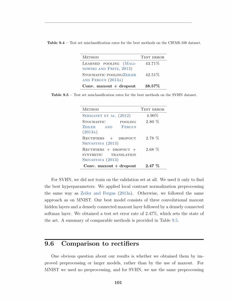
Table 9.4 – Test set misclassification rates for the best methods on the CIFAR-100 dataset.
Method Test error
Learned pooling (Mali-nowski and Fritz, 2013)
43.71%
Stochastic poolingZeilerand Fergus (2013a)
42.51%
Conv. maxout + dropout 38.57%
Table 9.5 – Test set misclassification rates for the best methods on the SVHN dataset.
Method Test error
Sermanet et al. (2012) 4.90%
Stochastic poolingZeiler and Fergus(2013a)
2.80 %
Rectifiers + dropoutSrivastava (2013)
2.78 %
Rectifiers + dropout +synthetic translationSrivastava (2013)
2.68 %
Conv. maxout + dropout 2.47 %
For SVHN, we did not train on the validation set at all. We used it only to find
the best hyperparameters. We applied local contrast normalization preprocessing
the same way as Zeiler and Fergus (2013a). Otherwise, we followed the same
approach as on MNIST. Our best model consists of three convolutional maxout
hidden layers and a densely connected maxout layer followed by a densely connected
softmax layer. We obtained a test set error rate of 2.47%, which sets the state of
the art. A summary of comparable methods is provided in Table 9.5.
9.6 Comparison to rectifiers
One obvious question about our results is whether we obtained them by im-
proved preprocessing or larger models, rather than by the use of maxout. For
MNIST we used no preprocessing, and for SVHN, we use the same preprocessing
101
as Zeiler and Fergus (2013a). However on the CIFAR datasets we did use a new
form of preprocessing. We therefore compare maxout to rectifiers run with the
same processing and a variety of model sizes on this dataset.
By running a large cross-validation experiment (see Fig. 9.6) we found that
maxout o↵ers a clear improvement over rectifiers. We also found that our pre-
processing and size of models improves rectifiers and dropout beyond the previous
state of the art result. Cross-channel pooling is a method for reducing the size of
state and number of parameters needed to have a given number of filters in the
model. Performance seems to correlate well with the number of filters for maxout
but with the number of output units for rectifiers–i.e, rectifier units do not benefit
much from cross-channel pooling. Rectifier units do best without cross-channel
pooling but with the same number of filters, meaning that the size of the state
and the number of parameters must be about k times higher for rectifiers to obtain
generalization performance approaching that of maxout.
9.7 Model averaging
Having demonstrated that maxout networks are e↵ective models, we now ana-
lyze the reasons for their success. We first identify reasons that maxout is highly
compatible with dropout’s approximate model averaging technique.
The intuitive justification for averaging sub-models by dividing the weights
by 2 given by (Hinton et al., 2012) is that this does exact model averaging for
a single layer model, softmax regression. To this characterization, we add the
observation that the model averaging remains exact if the model is extended to
multiple linear layers. While this has the same representational power as a single
layer, the expression of the weights as a product of several matrices could have
a di↵erent inductive bias. More importantly, it indicates that dropout does exact
model averaging in deeper architectures provided that they are locally linear among
the space of inputs to each layer that are visited by applying di↵erent dropout
masks.
We argue that dropout training encourages maxout units to have large linear
regions around inputs that appear in the training data. Because each sub-model
must make a good prediction of the output, each unit should learn to have roughly
102

the same activation regardless of which inputs are dropped. In a maxout network
with arbitrarily selected parameters, varying the dropout mask will often move
the e↵ective inputs far enough to escape the local region surrounding the clean
inputs in which the hidden units are linear, i.e., changing the dropout mask could
frequently change which piece of the piecewise function an input is mapped to.
Maxout trained with dropout may have the identity of the maximal filter in each
unit change relatively rarely as the dropout mask changes. Networks of linear
operations and max(·) may learn to exploit dropout’s approximate model averaging
technique well.
Many popular activation functions have significant curvature nearly everywhere.
These observations suggest that the approximate model averaging of dropout will
not be as accurate for networks incorporating such activation functions. To test
this, we compared the best maxout model trained on MNIST with dropout to a
hyperbolic tangent network trained on MNIST with dropout. We sampled several
subsets of each model and compared the geometric mean of these sampled mod-
els’ predictions to the prediction made using the dropout technique of dividing the
weights by 2. We found evidence that dropout is indeed performing model averag-
ing, even in multilayer networks, and that it is more accurate in the case of maxout.
See Fig. 9.7 and Fig. 9.8 for details.
9.8 Optimization
The second key reason that maxout performs well is that it improves the bagging
style training phase of dropout. Note that the arguments in section 9.7 motivating
the use of maxout also apply equally to rectified linear units (Salinas and Abbott,
1996; Hahnloser, 1998; Glorot et al., 2011). The only di↵erence between maxout
and max pooling over a set of rectified linear units is that maxout does not include
a 0 in the max. Superficially, this seems to be a small di↵erence, but we find that
including this constant 0 is very harmful to optimization in the context of dropout.
For instance, on MNIST our best validation set error with an MLP is 1.04%. If we
include a 0 in the max, this rises to over 1.2%. We argue that, when trained with
dropout, maxout is easier to optimize than rectified linear units with cross-channel
pooling.
103
9.8.1 Optimization experiments
To verify that maxout yields better optimization performance than max pooled
rectified linear units when training with dropout, we carried out two experiments.
First, we stressed the optimization capabilities of the training algorithm by training
a small (two hidden convolutional layers with k = 2 and sixteen kernels) model on
the large (600,000 example) SVHN dataset. When training with rectifier units the
training error gets stuck at 7.3%. If we train instead with maxout units, we obtain
5.1% training error. As another optimization stress test, we tried training very
deep and narrow models on MNIST, and found that maxout copes better with
increasing depth than pooled rectifiers. See Fig. 9.9 for details.
9.8.2 Saturation
Optimization proceeds very di↵erently when using dropout than when using
ordinary stochastic gradient descent. SGD usually works best with a small learn-
ing rate that results in a smoothly decreasing objective function, while dropout
works best with a large learning rate, resulting in a constantly fluctuating objec-
tive function. Dropout rapidly explores many di↵erent directions and rejects the
ones that worsen performance, while SGD moves slowly and steadily in the most
promising direction. We find empirically that these di↵erent operating regimes
result in di↵erent outcomes for rectifier units. When training with SGD, we find
that the rectifier units saturate at 0 less than 5% of the time. When training with
dropout, we initialize the units to sature rarely but training gradually increases
their saturation rate to 60%. Because the 0 in the max(0, z) activation function is
a constant, this blocks the gradient from flowing through the unit. In the absence of
gradient through the unit, it is di�cult for training to change this unit to become
active again. Maxout does not su↵er from this problem because gradient always
flows through every maxout unit–even when a maxout unit is 0, this 0 is a function
of the parameters and may be adjusted Units that take on negative activations
may be steered to become positive again later. Fig. 9.10 illustrates how active
rectifier units become inactive at a greater rate than inactive units become active
when training with dropout, but maxout units, which are always active, transition
between positive and negative activations at about equal rates in each direction.
We hypothesize that the high proportion of zeros and the di�culty of escaping
104
them impairs the optimization performance of rectifiers relative to maxout.
To test this hypothesis, we trained two MLPs on MNIST, both with two hidden
layers and 1200 filters per layer pooled in groups of 5. When we include a constant
0 in the max pooling, the resulting trained model fails to make use of 17.6% of
the filters in the second layer and 39.2% of the filters in the second layer. A small
minority of the filters usually took on the maximal value in the pool, and the rest
of the time the maximal value was a constant 0. Maxout, on the other hand, used
all but 2 of the 2400 filters in the network. Each filter in each maxout unit in the
network was maximal for some training example. All filters had been utilised and
tuned.
9.8.3 Lower layer gradients and bagging
To behave di↵erently from SGD, dropout requires the gradient to change notice-
ably as the choice of which units to drop changes. If the gradient is approximately
constant with respect to the dropout mask, then dropout simplifies to SGD training.
We tested the hypothesis that rectifier networks su↵er from diminished gradient
flow to the lower layers of the network by monitoring the variance with respect to
dropout masks for fixed data during training of two di↵erent MLPs on MNIST.
The variance of the gradient on the output weights was 1.4 times larger for maxout
on an average training step, while the variance on the gradient of the first layer
weights was 3.4 times larger for maxout than for rectifiers. Combined with our
previous result showing that maxout allows training deeper networks, this greater
variance suggests that maxout better propagates varying information downward
to the lower layers and helps dropout training to better resemble bagging for the
lower-layer parameters. Rectifier networks, with more of their gradient lost to sat-
uration, presumably cause dropout training to resemble regular SGD toward the
bottom of the network.
9.9 Conclusion
We have proposed a new activation function called maxout that is particularly
well suited for training with dropout, and for which we have proven a universal
approximation theorem. We have shown empirical evidence that dropout attains
105
a good approximation to model averaging in deep models. We have shown that
maxout exploits this model averaging behavior because the approximation is more
accurate for maxout units than for tanh units. We have demonstrated that opti-
mization behaves very di↵erently in the context of dropout than in the pure SGD
case. By designing the maxout gradient to avoid pitfalls such as failing to use
many of a model’s filters, we are able to train deeper networks than is possible
using rectifier units. We have also shown that maxout propagates variations in
the gradient due to di↵erent choices of dropout masks to the lowest layers of a
network, ensuring that every parameter in the model can enjoy the full benefit of
dropout and more faithfully emulate bagging training. The state of the art per-
formance of our approach on five di↵erent benchmark tasks motivates the design
of further models that are explicitly intended to perform well when combined with
inexpensive approximations to model averaging.
Acknowledgements
The authors would like to thank the developers of Theano (Bergstra et al.,
2010; Bastien et al., 2012), in particular Frederic Bastien and Pascal Lamblin for
their assistance with infrastructure development and performance optimization.
We would also like to thank Yann Dauphin for helpful discussions.
106
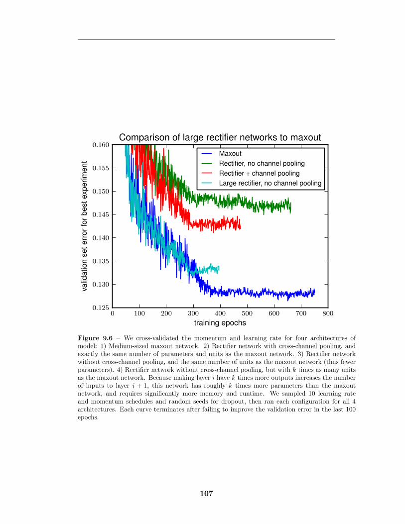
0 100 200 300 400 500 600 700 800
training epochs
0.125
0.130
0.135
0.140
0.145
0.150
0.155
0.160
valid
atio
nse
terr
orfo
rbes
texp
erim
ent
Comparison of large rectifier networks to maxout
MaxoutRectifier, no channel poolingRectifier + channel poolingLarge rectifier, no channel pooling
Figure 9.6 – We cross-validated the momentum and learning rate for four architectures ofmodel: 1) Medium-sized maxout network. 2) Rectifier network with cross-channel pooling, andexactly the same number of parameters and units as the maxout network. 3) Rectifier networkwithout cross-channel pooling, and the same number of units as the maxout network (thus fewerparameters). 4) Rectifier network without cross-channel pooling, but with k times as many unitsas the maxout network. Because making layer i have k times more outputs increases the numberof inputs to layer i + 1, this network has roughly k times more parameters than the maxoutnetwork, and requires significantly more memory and runtime. We sampled 10 learning rateand momentum schedules and random seeds for dropout, then ran each configuration for all 4architectures. Each curve terminates after failing to improve the validation error in the last 100epochs.
107
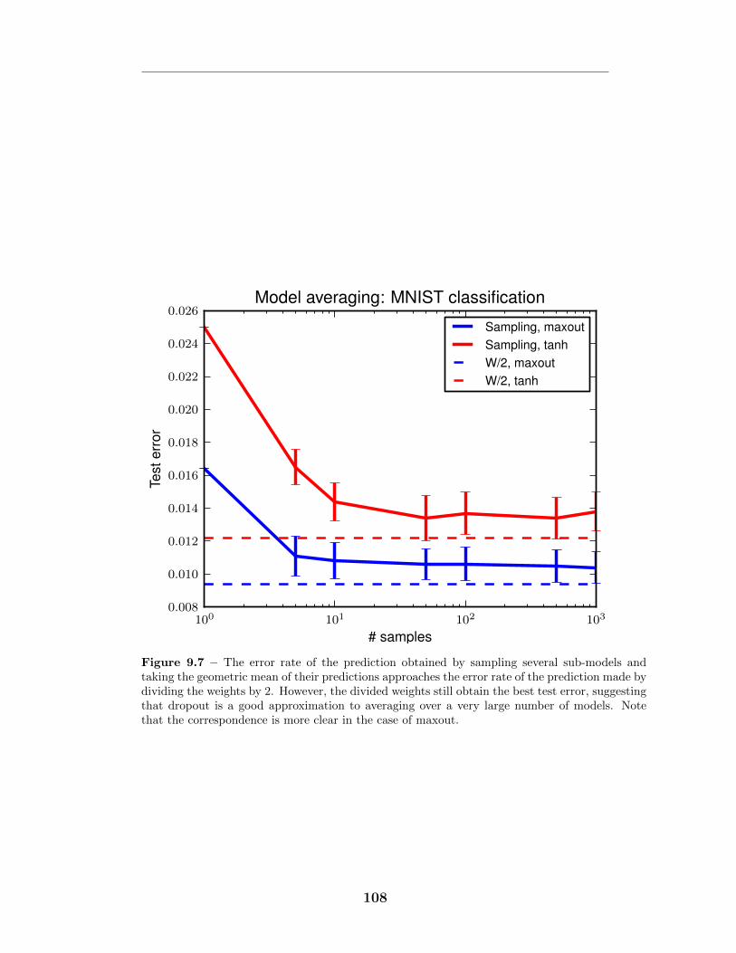
10
0
10
1
10
2
10
3
# samples
0.008
0.010
0.012
0.014
0.016
0.018
0.020
0.022
0.024
0.026
Test
erro
r
Model averaging: MNIST classification
Sampling, maxoutSampling, tanhW/2, maxoutW/2, tanh
Figure 9.7 – The error rate of the prediction obtained by sampling several sub-models andtaking the geometric mean of their predictions approaches the error rate of the prediction made bydividing the weights by 2. However, the divided weights still obtain the best test error, suggestingthat dropout is a good approximation to averaging over a very large number of models. Notethat the correspondence is more clear in the case of maxout.
108
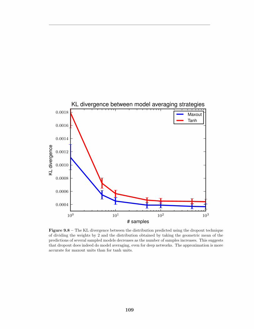
10
0
10
1
10
2
10
3
# samples
0.0004
0.0006
0.0008
0.0010
0.0012
0.0014
0.0016
0.0018
KL
dive
rgen
ce
KL divergence between model averaging strategies
MaxoutTanh
Figure 9.8 – The KL divergence between the distribution predicted using the dropout techniqueof dividing the weights by 2 and the distribution obtained by taking the geometric mean of thepredictions of several sampled models decreases as the number of samples increases. This suggeststhat dropout does indeed do model averaging, even for deep networks. The approximation is moreaccurate for maxout units than for tanh units.
109
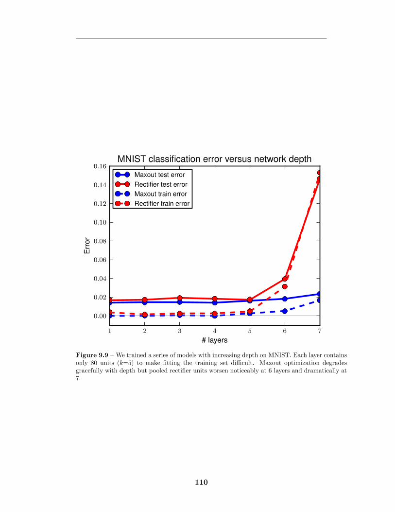
1 2 3 4 5 6 7
# layers
0.00
0.02
0.04
0.06
0.08
0.10
0.12
0.14
0.16
Err
or
MNIST classification error versus network depth
Maxout test errorRectifier test errorMaxout train errorRectifier train error
Figure 9.9 – We trained a series of models with increasing depth on MNIST. Each layer containsonly 80 units (k=5) to make fitting the training set di�cult. Maxout optimization degradesgracefully with depth but pooled rectifier units worsen noticeably at 6 layers and dramatically at7.
110
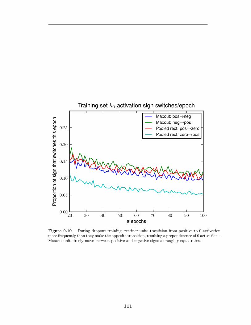
20 30 40 50 60 70 80 90 100
# epochs
0.00
0.05
0.10
0.15
0.20
0.25
Pro
porti
onof
sign
that
switc
hes
this
epoc
h
Training set h0 activation sign switches/epoch
Maxout: pos�negMaxout: neg�posPooled rect: pos�zeroPooled rect: zero�pos
Figure 9.10 – During dropout training, rectifier units transition from positive to 0 activationmore frequently than they make the opposite transition, resulting a preponderence of 0 activations.Maxout units freely move between positive and negative signs at roughly equal rates.
111

10 Prologue to Fourth Article
10.1 Article Details
Multi-digit number recognition from Street View imagery using deep
convolutional neural networks. Ian J. Goodfellow, Yaroslav Bulatov, Julian
Ibarz, Sacha Arnoud, and Vinay Shet (2014). In International Conference on
Learning Representations.
Personal Contribution. Because this article was written in the context of an
internship with the Street Smart team at Google, my personal contribution to this
article was less than to the other articles used in this thesis. The rest of the Street
Smart team already had the basic idea of doing transcription with a single neural
net before I arrived, and ran the experiments necessary for scientific publication
after I left. My main contribution was to clearly define the equations needed for
maximum likelihood training and MAP inference in the output sequence model, to
write the code for those features, and to configure the system for good performance
on the internal, private dataset. I did not perform any of the experiments designed
to explain the factors driving the success of the system, nor did I do any of the
work on the publicly available dataset.
10.2 Context
Prior to this work, no results had been published for the full sequence tran-
scription task on the Street View House Numbers dataset. Previous work, such
as that presented in chapter 9, had exclusively focused on the isolated digit recog-
nition task. Viable technologies already existed for sequence transcription, but
were mostly evaluated on other datasets. These technologies were not based on
learning to perform localization and segmentation in a single neural network, but
112
rather employed hand-designed probabilistic models that sometimes used neural
networks to implement individual conditional probability distributions within the
model. See (Alsharif and Pineau, 2013) for an example of a recent state of the art
system employing this approach.
We reproduce the paper here as it appeared in ICLR in its original form. How-
ever, it should be stressed that the ICLR version was written as a conference paper
and as such emphasized recent references. This work in fact builds on a very long
history of work on sequence recognition using convolutional neural networks. See
for example (Matan et al., 1992; Burges et al., 1992; Bengio et al., 1995; Schenkel
et al., 1993; LeCun and Bengio, 1994; Schenkel et al., 1995; Guyon et al., 1996; Bot-
tou et al., 1996, 1997; LeCun et al., 1997; LeCun et al., 1998; Bottou and LeCun,
2005).
10.3 Contributions
The contribution of this paper is twofold. First, we demonstrate a solution
to the problem of short sequence transcription for geocoding. Second, in doing
so, we have shown that deep neural networks can learn to perform complicated
localization and segmentation tasks rather than simply recognition tasks.
10.4 Recent Developments
This paper is very recent, and will in fact not be presented until after the writing
of this thesis. There are therefore no more recent developments to report.
113
11
Multi-digit Number
Recognition from Street
View Imagery using Deep
Convolutional Neural
Networks
11.1 Introduction
Recognizing multi-digit numbers in photographs captured at street level is an
important component of modern-day map making. A classic example of a cor-
pus of such street level photographs is Google’s Street View imagery comprised of
hundreds of millions of geo-located 360 degree panoramic images. The ability to
automatically transcribe an address number from a geo-located patch of pixels and
associate the transcribed number with a known street address helps pinpoint, with
a high degree of accuracy, the location of the building it represents.
More broadly, recognizing numbers in photographs is a problem of interest to
the optical character recognition community. While OCR on constrained domains
like document processing is well studied, arbitrary multi-character text recognition
in photographs is still highly challenging. This di�culty arises due to the wide
variability in the visual appearance of text in the wild on account of a large range
of fonts, colors, styles, orientations, and character arrangements. The recognition
problem is further complicated by environmental factors such as lighting, shad-
ows, specularities, and occlusions as well as by image acquisition factors such as
resolution, motion, and focus blurs.
In this paper, we focus on recognizing multi-digit numbers from Street View
panoramas. While this reduces the space of characters that need to be recognized,
the complexities listed above still apply to this sub-domain. Due to these com-
plexities, traditional approaches to solve this problem typically separate out the
localization, segmentation, and recognition steps.
In this paper we propose a unified approach that integrates these three steps
via the use of a deep convolutional neural network that operates directly on the
image pixels. This model is configured with multiple hidden layers (our best con-
figuration had eleven layers, but our experiments suggest deeper architectures may
114
obtain better accuracy, with diminishing returns), all with feedforward connections.
We employ DistBelief to implement these large-scale deep neural networks. The
key contributions of this paper are: (a) a unified model to localize, segment, and
recognize multi-digit numbers from street level photographs (b) a new kind of out-
put layer, providing a conditional probabilistic model of sequences (c) empirical
results that show this model performing best with a deep architecture (d) reaching
human level performance at specific operating thresholds.
We have evaluated this approach on the publicly available Street View House
Numbers (SVHN) dataset and achieve over 96% accuracy in recognizing street
numbers. We show that on a per-digit recognition task, we improve upon the state-
of-the-art and achieve 97.84% accuracy. We also evaluated this approach on an even
more challenging dataset generated from Street View imagery containing several
tens of millions of street number annotations and achieve over 90% accuracy. Our
evaluations further indicate that at specific operating thresholds, the performance
of the proposed system is comparable to that of human operators. To date, our
system has helped us extract close to 100 million street numbers from Street View
imagery worldwide.
The rest of the paper is organized as follows: Section 11.2 explores past work on
deep neural networks and on Photo-OCR. Sections 11.3 and 11.4 list the problem
definition and describe the proposed method. Section 11.5 describes the experi-
mental set up and results. Key takeaway ideas are discussed in Section 11.6.
11.2 Related work
Convolutional neural networks (Fukushima, 1980; LeCun et al., 1998) are neural
networks with sets of neurons having tied parameters. Like most neural networks,
they contain several filtering layers with each layer applying an a�ne transforma-
tion to the vector input followed by an elementwise non-linearity. In the case of
convolutional networks, the a�ne transformation can be implemented as a discrete
convolution rather than a fully general matrix multiplication. This makes convo-
lutional networks computationally e�cient, allowing them to scale to large images.
It also builds equivariance to translation into the model (in other words, if the
image is shifted by one pixel to the right, then the output of the convolution is
115
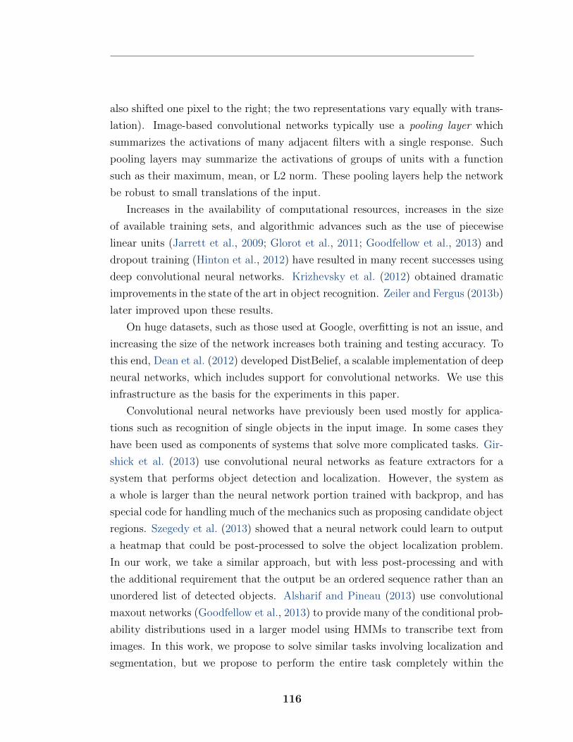
also shifted one pixel to the right; the two representations vary equally with trans-
lation). Image-based convolutional networks typically use a pooling layer which
summarizes the activations of many adjacent filters with a single response. Such
pooling layers may summarize the activations of groups of units with a function
such as their maximum, mean, or L2 norm. These pooling layers help the network
be robust to small translations of the input.
Increases in the availability of computational resources, increases in the size
of available training sets, and algorithmic advances such as the use of piecewise
linear units (Jarrett et al., 2009; Glorot et al., 2011; Goodfellow et al., 2013) and
dropout training (Hinton et al., 2012) have resulted in many recent successes using
deep convolutional neural networks. Krizhevsky et al. (2012) obtained dramatic
improvements in the state of the art in object recognition. Zeiler and Fergus (2013b)
later improved upon these results.
On huge datasets, such as those used at Google, overfitting is not an issue, and
increasing the size of the network increases both training and testing accuracy. To
this end, Dean et al. (2012) developed DistBelief, a scalable implementation of deep
neural networks, which includes support for convolutional networks. We use this
infrastructure as the basis for the experiments in this paper.
Convolutional neural networks have previously been used mostly for applica-
tions such as recognition of single objects in the input image. In some cases they
have been used as components of systems that solve more complicated tasks. Gir-
shick et al. (2013) use convolutional neural networks as feature extractors for a
system that performs object detection and localization. However, the system as
a whole is larger than the neural network portion trained with backprop, and has
special code for handling much of the mechanics such as proposing candidate object
regions. Szegedy et al. (2013) showed that a neural network could learn to output
a heatmap that could be post-processed to solve the object localization problem.
In our work, we take a similar approach, but with less post-processing and with
the additional requirement that the output be an ordered sequence rather than an
unordered list of detected objects. Alsharif and Pineau (2013) use convolutional
maxout networks (Goodfellow et al., 2013) to provide many of the conditional prob-
ability distributions used in a larger model using HMMs to transcribe text from
images. In this work, we propose to solve similar tasks involving localization and
segmentation, but we propose to perform the entire task completely within the
116
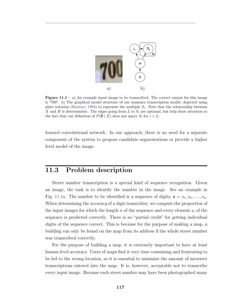
X
H
L SiN
a) b)
Figure 11.1 – a) An example input image to be transcribed. The correct output for this imageis “700”. b) The graphical model structure of our sequence transcription model, depicted usingplate notation (Buntine, 1994) to represent the multiple Si. Note that the relationship betweenX and H is deterministic. The edges going from L to Si are optional, but help draw attention tothe fact that our definition of P (S | X) does not query Si for i > L.
learned convolutional network. In our approach, there is no need for a separate
component of the system to propose candidate segmentations or provide a higher
level model of the image.
11.3 Problem description
Street number transcription is a special kind of sequence recognition. Given
an image, the task is to identify the number in the image. See an example in
Fig. 11.1a. The number to be identified is a sequence of digits, s = s1
, s2
, . . . , sn
.
When determining the accuracy of a digit transcriber, we compute the proportion of
the input images for which the length n of the sequence and every element si
of the
sequence is predicted correctly. There is no “partial credit” for getting individual
digits of the sequence correct. This is because for the purpose of making a map, a
building can only be found on the map from its address if the whole street number
was transcribed correctly.
For the purpose of building a map, it is extremely important to have at least
human level accuracy. Users of maps find it very time consuming and frustrating to
be led to the wrong location, so it is essential to minimize the amount of incorrect
transcriptions entered into the map. It is, however, acceptable not to transcribe
every input image. Because each street number may have been photographed many
117
times, it is still quite likely that the proportion of buildings we can place on the map
is greater than the proportion of images we can transcribe. We therefore advocate
evaluating this task based on the coverage at certain levels of accuracy, rather than
evaluating only the total degree of accuracy of the system. To evaluate coverage,
the system must return a confidence value, such as the probability of the most likely
prediction being correct. Transcriptions below some confidence threshold can then
be discarded. The coverage is defined to be the proportion of inputs that are not
discarded. The coverage at a certain specific accuracy level is the coverage that
results when the confidence threshold is chosen to achieve that desired accuracy
level. For map-making purposes, we are primarily interested in coverage at 98%
accuracy or better, since this roughly corresponds to human accuracy.
Using confidence thresholding allows us to improve maps incrementally over
time–if we develop a system with poor accuracy overall but good accuracy at some
threshold, we can make a map with partial coverage, then improve the coverage
when we get a more accurate transcription system in the future. We can also use
confidence thresholding to do as much of the work as possible via the automated
system and do the rest using more expensive means such as hiring human operators
to transcribe the remaining di�cult inputs.
One special property of the street number transcription problem is that the
sequences are of bounded length. Very few street numbers contain more than five
digits, so we can use models that assume the sequence length n is at most some
constant N , with N = 5 for this work. Systems that make such an assumption
should be able to identify whenever this assumption is violated and refuse to re-
turn a transcription so that the few street numbers of length greater than N are
not incorrectly added to the map after being transcribed as being length N . (Al-
ternately, one can return the most likely sequence of length N , and because the
probability of that transcription being correct is low, the default confidence thresh-
olding mechanism will usually reject such transcriptions without needing special
code for handling the excess length case)
118
11.4 Methods
Our basic approach is to train a probabilistic model of sequences given images.
Let S represent the output sequence and X represent the input image. Our goal is
then to learn a model of P (S | X) by maximizing log P (S | X) on the training set.
To model S, we define S as a collection of N random variables S1
, . . . , SN
representing the elements of the sequence and an additional random variable L
representing the length of the sequence. We assume that the identities of the
separate digits are independent from each other, so that the probability of a specific
sequence s = s1
, . . . , sn
is given by
P (S = s|X) = P (L = n | X)⇧n
i=1
P (Si
= si
| X).
This model can be extended to detect when our assumption that the sequence has
length at most N is violated. To allow for detecting this case, we simply add an
additional value of L that represents this outcome.
Each of the variables above is discrete, and when applied to the street number
transcription problem, each has a small number of possible values: L has only 7
values (0, . . . , 5, and “more than 5”), and each of the digit variables has 10 possible
values. This means it is feasible to represent each of them with a softmax classifier
that receives as input features extracted from X by a convolutional neural network.
We can represent these features as a random variable H whose value is deterministic
given X. In this model, P (S | X) = P (S | H). See Fig. 11.1b for a graphical model
depiction of the network structure.
To train the model, one can maximize log P (S | X) on the training set using
a generic method like stochastic gradient descent. Each of the softmax models
(the model for L and each Si
) can use exactly the same backprop learning rule
as when training an isolated softmax layer, except that a digit classifier softmax
model backprops nothing on examples for which that digit is not present.
At test time, we predict
s = (l, s1
, . . . , sl
) = argmaxL,S
1
,...,SLlog P (S | X).
This argmax can be computed in linear time. The argmax for each character can
be computed independently. We then incrementally add up the log probabilities
for each character. For each length l, the complete log probability is given by this
running sum of character log probabilities, plus log P (l | x). The total runtime is
119
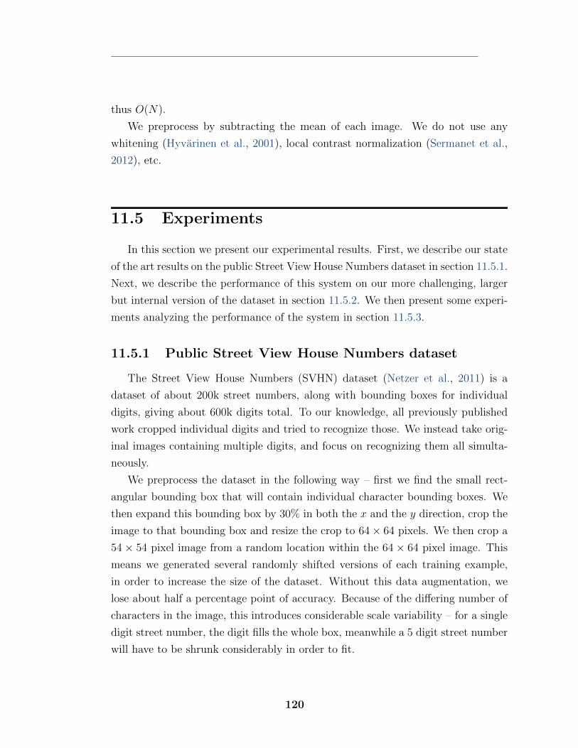
thus O(N).
We preprocess by subtracting the mean of each image. We do not use any
whitening (Hyvarinen et al., 2001), local contrast normalization (Sermanet et al.,
2012), etc.
11.5 Experiments
In this section we present our experimental results. First, we describe our state
of the art results on the public Street View House Numbers dataset in section 11.5.1.
Next, we describe the performance of this system on our more challenging, larger
but internal version of the dataset in section 11.5.2. We then present some experi-
ments analyzing the performance of the system in section 11.5.3.
11.5.1 Public Street View House Numbers dataset
The Street View House Numbers (SVHN) dataset (Netzer et al., 2011) is a
dataset of about 200k street numbers, along with bounding boxes for individual
digits, giving about 600k digits total. To our knowledge, all previously published
work cropped individual digits and tried to recognize those. We instead take orig-
inal images containing multiple digits, and focus on recognizing them all simulta-
neously.
We preprocess the dataset in the following way – first we find the small rect-
angular bounding box that will contain individual character bounding boxes. We
then expand this bounding box by 30% in both the x and the y direction, crop the
image to that bounding box and resize the crop to 64 ⇥ 64 pixels. We then crop a
54 ⇥ 54 pixel image from a random location within the 64 ⇥ 64 pixel image. This
means we generated several randomly shifted versions of each training example,
in order to increase the size of the dataset. Without this data augmentation, we
lose about half a percentage point of accuracy. Because of the di↵ering number of
characters in the image, this introduces considerable scale variability – for a single
digit street number, the digit fills the whole box, meanwhile a 5 digit street number
will have to be shrunk considerably in order to fit.
120
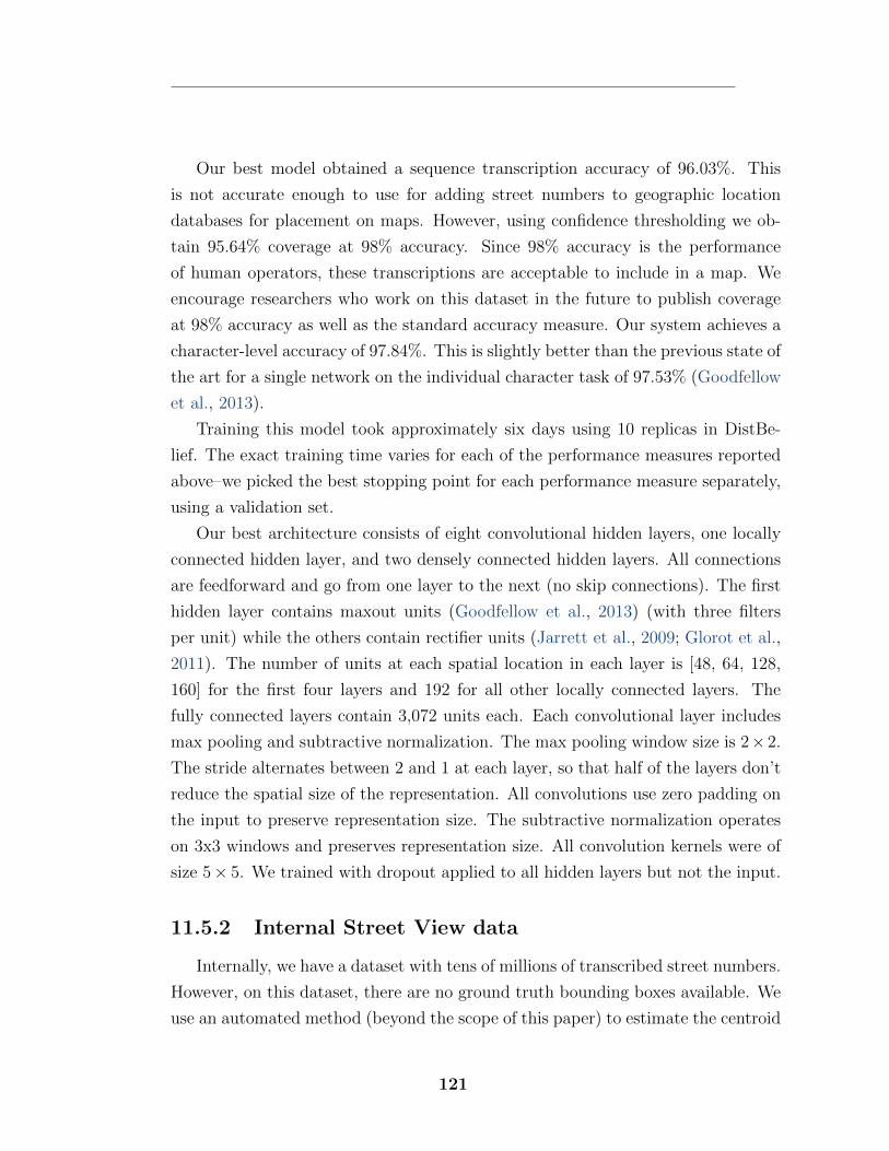
Our best model obtained a sequence transcription accuracy of 96.03%. This
is not accurate enough to use for adding street numbers to geographic location
databases for placement on maps. However, using confidence thresholding we ob-
tain 95.64% coverage at 98% accuracy. Since 98% accuracy is the performance
of human operators, these transcriptions are acceptable to include in a map. We
encourage researchers who work on this dataset in the future to publish coverage
at 98% accuracy as well as the standard accuracy measure. Our system achieves a
character-level accuracy of 97.84%. This is slightly better than the previous state of
the art for a single network on the individual character task of 97.53% (Goodfellow
et al., 2013).
Training this model took approximately six days using 10 replicas in DistBe-
lief. The exact training time varies for each of the performance measures reported
above–we picked the best stopping point for each performance measure separately,
using a validation set.
Our best architecture consists of eight convolutional hidden layers, one locally
connected hidden layer, and two densely connected hidden layers. All connections
are feedforward and go from one layer to the next (no skip connections). The first
hidden layer contains maxout units (Goodfellow et al., 2013) (with three filters
per unit) while the others contain rectifier units (Jarrett et al., 2009; Glorot et al.,
2011). The number of units at each spatial location in each layer is [48, 64, 128,
160] for the first four layers and 192 for all other locally connected layers. The
fully connected layers contain 3,072 units each. Each convolutional layer includes
max pooling and subtractive normalization. The max pooling window size is 2⇥2.
The stride alternates between 2 and 1 at each layer, so that half of the layers don’t
reduce the spatial size of the representation. All convolutions use zero padding on
the input to preserve representation size. The subtractive normalization operates
on 3x3 windows and preserves representation size. All convolution kernels were of
size 5 ⇥ 5. We trained with dropout applied to all hidden layers but not the input.
11.5.2 Internal Street View data
Internally, we have a dataset with tens of millions of transcribed street numbers.
However, on this dataset, there are no ground truth bounding boxes available. We
use an automated method (beyond the scope of this paper) to estimate the centroid
121
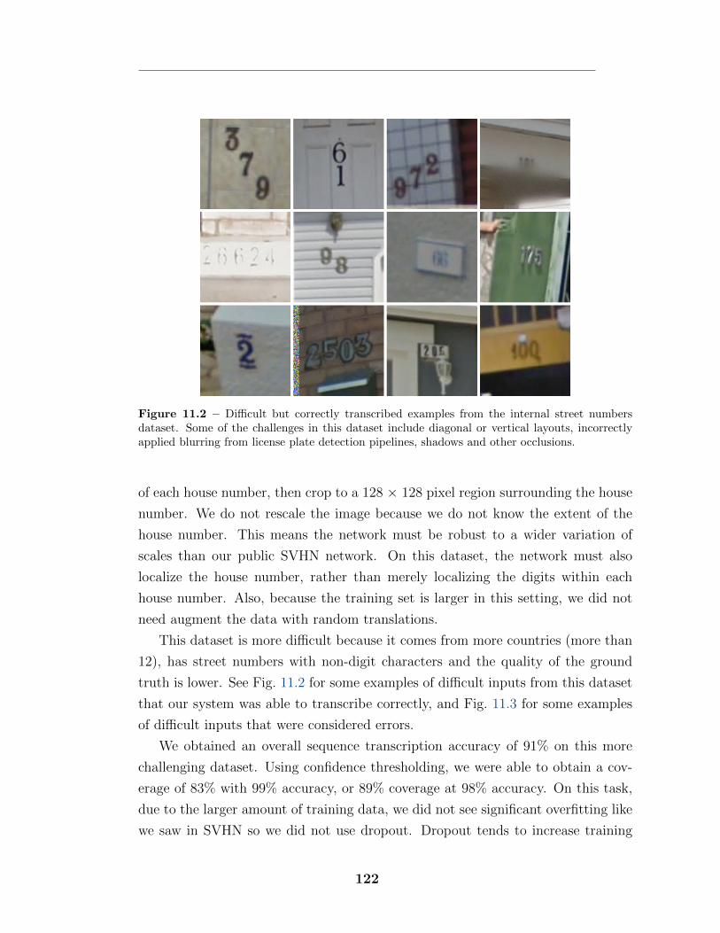
Figure 11.2 – Di�cult but correctly transcribed examples from the internal street numbersdataset. Some of the challenges in this dataset include diagonal or vertical layouts, incorrectlyapplied blurring from license plate detection pipelines, shadows and other occlusions.
of each house number, then crop to a 128 ⇥ 128 pixel region surrounding the house
number. We do not rescale the image because we do not know the extent of the
house number. This means the network must be robust to a wider variation of
scales than our public SVHN network. On this dataset, the network must also
localize the house number, rather than merely localizing the digits within each
house number. Also, because the training set is larger in this setting, we did not
need augment the data with random translations.
This dataset is more di�cult because it comes from more countries (more than
12), has street numbers with non-digit characters and the quality of the ground
truth is lower. See Fig. 11.2 for some examples of di�cult inputs from this dataset
that our system was able to transcribe correctly, and Fig. 11.3 for some examples
of di�cult inputs that were considered errors.
We obtained an overall sequence transcription accuracy of 91% on this more
challenging dataset. Using confidence thresholding, we were able to obtain a cov-
erage of 83% with 99% accuracy, or 89% coverage at 98% accuracy. On this task,
due to the larger amount of training data, we did not see significant overfitting like
we saw in SVHN so we did not use dropout. Dropout tends to increase training
122
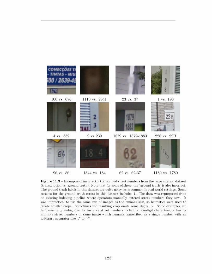
100 vs. 676 1110 vs. 2641 23 vs. 37 1 vs. 198
4 vs. 332 2 vs 239 1879 vs. 1879-1883 228 vs. 22B
96 vs. 86 1844 vs. 184 62 vs. 62-37 1180 vs. 1780
Figure 11.3 – Examples of incorrectly transcribed street numbers from the large internal dataset(transcription vs. ground truth). Note that for some of these, the “ground truth” is also incorrect.The ground truth labels in this dataset are quite noisy, as is common in real world settings. Somereasons for the ground truth errors in this dataset include: 1. The data was repurposed froman existing indexing pipeline where operators manually entered street numbers they saw. Itwas impractical to use the same size of images as the humans saw, so heuristics were used tocreate smaller crops. Sometimes the resulting crop omits some digits. 2. Some examples arefundamentally ambiguous, for instance street numbers including non-digit characters, or havingmultiple street numbers in same image which humans transcribed as a single number with anarbitrary separator like “,” or “-”.
123
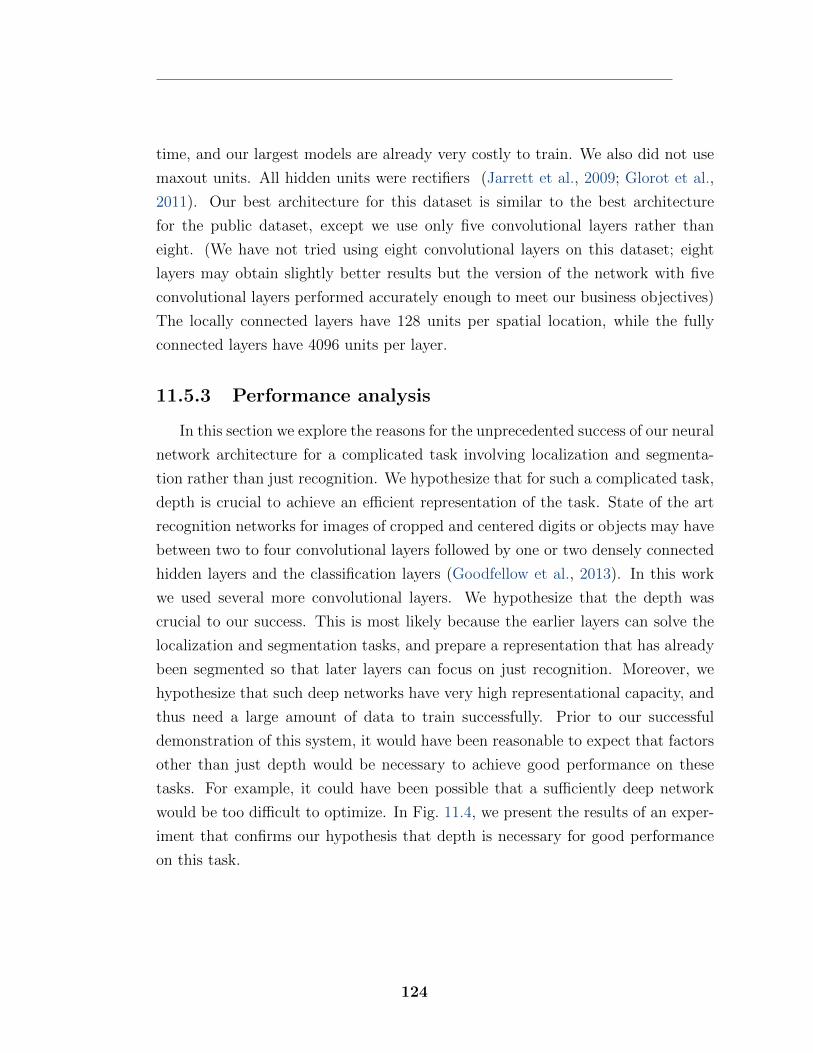
time, and our largest models are already very costly to train. We also did not use
maxout units. All hidden units were rectifiers (Jarrett et al., 2009; Glorot et al.,
2011). Our best architecture for this dataset is similar to the best architecture
for the public dataset, except we use only five convolutional layers rather than
eight. (We have not tried using eight convolutional layers on this dataset; eight
layers may obtain slightly better results but the version of the network with five
convolutional layers performed accurately enough to meet our business objectives)
The locally connected layers have 128 units per spatial location, while the fully
connected layers have 4096 units per layer.
11.5.3 Performance analysis
In this section we explore the reasons for the unprecedented success of our neural
network architecture for a complicated task involving localization and segmenta-
tion rather than just recognition. We hypothesize that for such a complicated task,
depth is crucial to achieve an e�cient representation of the task. State of the art
recognition networks for images of cropped and centered digits or objects may have
between two to four convolutional layers followed by one or two densely connected
hidden layers and the classification layers (Goodfellow et al., 2013). In this work
we used several more convolutional layers. We hypothesize that the depth was
crucial to our success. This is most likely because the earlier layers can solve the
localization and segmentation tasks, and prepare a representation that has already
been segmented so that later layers can focus on just recognition. Moreover, we
hypothesize that such deep networks have very high representational capacity, and
thus need a large amount of data to train successfully. Prior to our successful
demonstration of this system, it would have been reasonable to expect that factors
other than just depth would be necessary to achieve good performance on these
tasks. For example, it could have been possible that a su�ciently deep network
would be too di�cult to optimize. In Fig. 11.4, we present the results of an exper-
iment that confirms our hypothesis that depth is necessary for good performance
on this task.
124
Figure 11.4 – Performance analysis experiments on the public SVHN dataset show that fairlydeep architectures are needed to obtain good performance on the sequence transcription task.
11.5.4 Application to Geocoding
The motivation for the development of this model was to decrease the cost of
geocoding as well as scale it worldwide and keep up with change in the world.
The model has now reached a high enough quality level that we can automate the
extraction of street numbers on Street View images. Also, even if the model can
be considered quite large, it is still e�cient.
We can for example transcribe all the views we have of street numbers in France
in less than an hour using our Google infrastructure. Most of the cost actually
comes from the detection stage that locates the street numbers in the large Street
View images. Worldwide, we automatically detected and transcribed close to 100
million physical street numbers at operator level accuracy. Having this new dataset
significantly increased the geocoding quality of Google Maps in several countries
especially the ones that did not already have other sources of good geocoding. In
Fig. 11.5, you can see some automatically extracted street numbers from Street
View imagery captured in South Africa.
125
11.6 Discussion
We believe with this model we have solved OCR for short sequences for many
applications. On our particular task, we believe that now the biggest gain we could
easily get is to increase the quality of the training set itself as well as increasing its
size for general OCR transcription.
One caveat to our results with this architecture is that they rest heavily on
the assumption that the sequence is of bounded length, with a reasonably small
maximum length N . For unbounded N , our method is not directly applicable,
and for large N our method is unlikely to scale well. Each separate digit classifier
requires its own separate weight matrix. For long sequences this could incur too
high of a memory cost. When using DistBelief, memory is not much of an issue
(just use more machines) but statistical e�ciency is likely to become problematic.
Another problem with long sequences is the cost function itself. It’s also possible
that, due to longer sequences having more digit probabilities multiplied together,
a model of longer sequences could have trouble with systematic underestimation of
the sequence length.
One possible solution could be to train a model that outputs one “word” (N
character sequence) at a time and then slide it over the entire image followed by a
simple decoding. Some early experiments in this direction have been promising.
Perhaps our most interesting finding is that neural networks can learn to per-
form complicated tasks such as simultaneous localization and segmentation of or-
dered sequences of objects. This approach of using a single neural network as an
entire end-to-end system could be applicable to other problems, such as general
text transcription or speech recognition.
126

Acknowledgments
We would like to thank Ilya Sutskever and Samy Bengio for helpful discussions.
We would also like to thank the entire operation team in India that did the labeling
e↵ort and without whom this research would not have been possible.
127

Figure 11.5 – Automatically extracted street numbers from Street View imagery captured inSouth Africa.
.
128
12 General conclusion
The work in this thesis has tracked the general change in the zeitgeist of deep
learning research that took place during the time it was written.
The projects begun earlier in the work for this thesis were based on the paradigm
of representation learning. The hypothesis guiding these works was that by learning
to represent the world, we might learn to reason about it more accurately, and
improve accuracy on supervised learning tasks. In the short run, that hypothesis
has proven to be of little value. The MP-DBM, trained simultaneously to model the
input and to predict the output, performs slightly better than a purely supervised
maxout network, but the improvement in accuracy is small compared to the increase
in complexity of the network.
Instead, we have found that averaging together large ensembles of models is a
much more powerful, and in the short term, feasible approach to improving the
generalization of models for computer vision. The success of the MP-DBM is
attributable in part to the fact that it trains an exponentially large ensemble of
recurrent networks. Likewise, the later projects in this thesis, leverage dropout to
train exponentially large ensembles of feedforward networks.
Similarly, it seems that in the short term it is much easier to collect large
amounts of data than to learn to generalize well from small amounts of data. Using
this strategy, we were able to automatically transcribe over one hundred million
address numbers from photos around the world.
This shift from representation learning to implicit ensembles and supervised
learning with large datasets has been an industry-wide phenomenon. This thesis
also highlights a few nuances of the overall findings of the research community over
the past few years. First, the experiments with S3C and small amounts of labeled
data show that representation learning is of some use when the amount of unlabeled
data greatly exceeds the amount of labeled data. However, these approaches are
not yet su�cient to succeed at AI-style tasks. The experiments with the MP-DBM
have also shown that generative models can still be useful even when su�cient
129
labeled data is available. The MP-DBM can replace missing input values and
can perform classification even when some inputs are missing. This suggests that
generative modeling may still be relevant even in the age of “big data.”
Finally, one lesson that can be gleaned from this thesis is that it is possible
to achieve powerful synergy in a machine learning system by designing each of its
components to interact well with each other. As engineers, we draw great benefit
from designing modular systems, with components that can be analyzed separately.
Machine learning systems can usually be broken into subsystems that represent
knowledge, subsystems that perform inference given the stored knowledge, and op-
timization procedures that inject new knowledge into the representation. Being
able to diagnose which of these subsystems performs the worst is usually the best
basis we have for determining how to improve a machine learning system. This
ability to consider the components in isolation is crucial to understanding machine
learning systems. But we should not forget to also consider their combined per-
formance. Maxout works well because it is a representation system that works
especially well with both the optimization procedure and the inference procedure
used when training with dropout. This general principle of seeking synergy be-
tween components that remain simple to analyze in isolation could lead to more
advances in other machine learning systems.
130
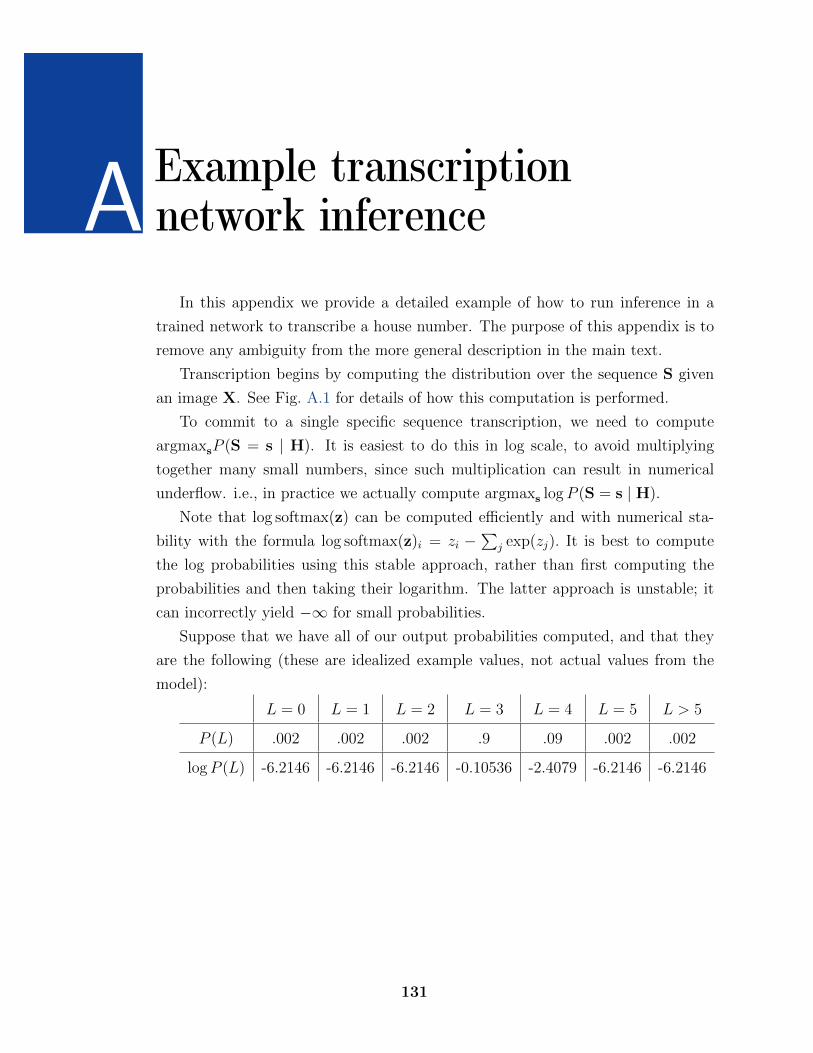
A Example transcription
network inference
In this appendix we provide a detailed example of how to run inference in a
trained network to transcribe a house number. The purpose of this appendix is to
remove any ambiguity from the more general description in the main text.
Transcription begins by computing the distribution over the sequence S given
an image X. See Fig. A.1 for details of how this computation is performed.
To commit to a single specific sequence transcription, we need to compute
argmaxs
P (S = s | H). It is easiest to do this in log scale, to avoid multiplying
together many small numbers, since such multiplication can result in numerical
underflow. i.e., in practice we actually compute argmaxs
log P (S = s | H).
Note that log softmax(z) can be computed e�ciently and with numerical sta-
bility with the formula log softmax(z)i
= zi
� Pj
exp(zj
). It is best to compute
the log probabilities using this stable approach, rather than first computing the
probabilities and then taking their logarithm. The latter approach is unstable; it
can incorrectly yield �1 for small probabilities.
Suppose that we have all of our output probabilities computed, and that they
are the following (these are idealized example values, not actual values from the
model):
L = 0 L = 1 L = 2 L = 3 L = 4 L = 5 L > 5
P (L) .002 .002 .002 .9 .09 .002 .002
log P (L) -6.2146 -6.2146 -6.2146 -0.10536 -2.4079 -6.2146 -6.2146
131
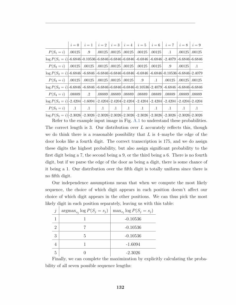
i = 0 i = 1 i = 2 i = 3 i = 4 i = 5 i = 6 i = 7 i = 8 i = 9
P (S1 = i) .00125 .9 .00125 .00125 .00125 .00125 .00125 .1 .00125 .00125
log P (S1 = i) -6.6846 -0.10536 -6.6846 -6.6846 -6.6846 -6.6846 -6.6846 -2.4079 -6.6846 -6.6846
P (S2 = i) .00125 .00125 .00125 .00125 .00125 .00125 .00125 .9 .00125 .1
log P (S2 = i) -6.6846 -6.6846 -6.6846 -6.6846 -6.6846 -6.6846 -6.6846 -0.10536 -6.6846 -2.4079
P (S3 = i) .00125 .00125 .00125 .00125 .00125 .9 .1 .00125 .00125 .00125
log P (S3 = i) -6.6846 -6.6846 -6.6846 -6.6846 -6.6846 -0.10536 -2.4079 -6.6846 -6.6846 -6.6846
P (S4 = i) .08889 .2 .08889 .08889 .08889 .08889 .08889 .08889 .08889 .08889
log P (S4 = i) -2.4204 -1.6094 -2.4204 -2.4204 -2.4204 -2.4204 -2.4204 -2.4204 -2.4204 -2.4204
P (S5 = i) .1 .1 .1 .1 .1 .1 .1 .1 .1 .1
log P (S5 = i) -2.3026 -2.3026 -2.3026 -2.3026 -2.3026 -2.3026 -2.3026 -2.3026 -2.3026 -2.3026
Refer to the example input image in Fig. A.1 to understand these probabilities.
The correct length is 3. Our distribution over L accurately reflects this, though
we do think there is a reasonable possibility that L is 4–maybe the edge of the
door looks like a fourth digit. The correct transcription is 175, and we do assign
these digits the highest probability, but also assign significant probability to the
first digit being a 7, the second being a 9, or the third being a 6. There is no fourth
digit, but if we parse the edge of the door as being a digit, there is some chance of
it being a 1. Our distribution over the fifth digit is totally uniform since there is
no fifth digit.
Our independence assumptions mean that when we compute the most likely
sequence, the choice of which digit appears in each position doesn’t a↵ect our
choice of which digit appears in the other positions. We can thus pick the most
likely digit in each position separately, leaving us with this table:
j argmaxsj
log P (Sj
= sj
) maxsj log P (S
j
= sj
)
1 1 -0.10536
2 7 -0.10536
3 5 -0.10536
4 1 -1.6094
5 0 -2.3026Finally, we can complete the maximization by explicitly calculating the proba-
bility of all seven possible sequence lengths:
132
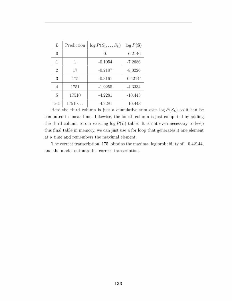
L Prediction log P (S1
, . . . SL
) log P (S)
0 0. -6.2146
1 1 -0.1054 -7.2686
2 17 -0.2107 -8.3226
3 175 -0.3161 -0.42144
4 1751 -1.9255 -4.3334
5 17510 -4.2281 -10.443
> 5 17510. . . -4.2281 -10.443
Here the third column is just a cumulative sum over log P (SL
) so it can be
computed in linear time. Likewise, the fourth column is just computed by adding
the third column to our existing log P (L) table. It is not even necessary to keep
this final table in memory, we can just use a for loop that generates it one element
at a time and remembers the maximal element.
The correct transcription, 175, obtains the maximal log probability of �0.42144,
and the model outputs this correct transcription.
133
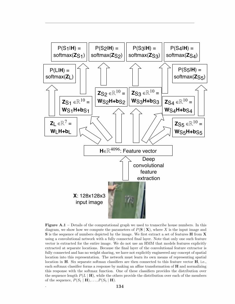
X: 128x128x3 input image
Deep convolutional
feature extraction
H∈�4096: Feature vector
ZS1 ∈�10 =WS1H+bS1
ZL ∈�7 =WLH+bL
ZS2 ∈�10 =WS2H+bS2
ZS3 ∈�10 =WS3H+bS3 ZS4 ∈�10 =
WS4H+bS4
ZS5 ∈�10 =WS5H+bS5
P(L|H) =softmax(ZL)
P(S1|H) =softmax(ZS1)
P(S2|H) =softmax(ZS2)
P(S3|H) =softmax(ZS3)
P(S4|H) =softmax(ZS4)
P(S5|H) =softmax(ZS5)
Figure A.1 – Details of the computational graph we used to transcribe house numbers. In thisdiagram, we show how we compute the parameters of P (S | X), where X is the input image andS is the sequence of numbers depicted by the image. We first extract a set of features H from Xusing a convolutional network with a fully connected final layer. Note that only one such featurevector is extracted for the entire image. We do not use an HMM that models features explicitlyextracted at separate locations. Because the final layer of the convolutional feature extractor isfully connected and has no weight sharing, we have not explicitly engineered any concept of spatiallocation into this representation. The network must learn its own means of representing spatiallocation in H. Six separate softmax classifiers are then connected to this feature vector H, i.e.,each softmax classifier forms a response by making an a�ne transformation of H and normalizingthis response with the softmax function. One of these classifiers provides the distribution overthe sequence length P (L | H), while the others provide the distribution over each of the membersof the sequence, P (S1 | H), . . . , P (S5 | H).
. 134
Bibliography
Alsharif, O. and J. Pineau (2013). End-to-end text recognition with hybrid HMM
maxout models. Technical report, arXiv:1310.1811.
Arnold, L. and Y. Ollivier (2012, December). Layer-wise learning of deep generative
models. Technical report, arXiv:1212.1524.
Bastien, F., P. Lamblin, R. Pascanu, J. Bergstra, I. J. Goodfellow, A. Bergeron,
N. Bouchard, and Y. Bengio (2012). Theano: new features and speed improve-
ments. Deep Learning and Unsupervised Feature Learning NIPS 2012 Workshop.
Bengio, Y. (2009). Learning deep architectures for AI. Foundations and Trends in
Machine Learning 2 (1), 1–127. Also published as a book. Now Publishers, 2009.
Bengio, Y., P. Lamblin, D. Popovici, and H. Larochelle (2007). Greedy layer-wise
training of deep networks. In B. Scholkopf, J. Platt, and T. Ho↵man (Eds.),
Advances in Neural Information Processing Systems 19 (NIPS’06), pp. 153–160.
MIT Press.
Bengio, Y., Y. LeCun, C. Nohl, and C. Burges (1995). Lerec: A NN/HMM hybrid
for on-line handwriting recognition. Neural Computation 7 (6), 1289–1303.
Bengio, Y., E. Thibodeau-Laufer, G. Alain, and J. Yosinski (2014). Deep generative
stochastic networks trainable by backprop. Technical Report arXiv:1306.1091.
Bergstra, J., O. Breuleux, F. Bastien, P. Lamblin, R. Pascanu, G. Desjardins,
J. Turian, D. Warde-Farley, and Y. Bengio (2010, June). Theano: a CPU and
GPU math expression compiler. In Proceedings of the Python for Scientific Com-
puting Conference (SciPy). Oral Presentation.
Bishop, C. M. (2006). Pattern Recognition and Machine Learning. Springer.
Blackwell, D. (1947). Conditional Expectation and Unbiased Sequential Estima-
tion. Ann.Math.Statist. 18, 105–110.
135
bo Duan, K. and S. S. Keerthi (2005). Which is the best multiclass SVM method?
an empirical study. In Proceedings of the Sixth International Workshop on Mul-
tiple Classifier Systems, pp. 278–285.
Bottou, L., Y. Bengio, and Y. A. Le Cun (1996, July). Document analysis with
generalized transduction. Technical Report HA6156000-960701-01TM, AT&T
Laboratories, Holmdel, New-Jersey.
Bottou, L., Y. Bengio, and Y. LeCun (1997). Global training of document process-
ing systems using graph transformer networks. In Proceedings of the Computer
Vision and Pattern Recognition Conference (CVPR’97), Puerto Rico, pp. 490–
494. IEEE.
Bottou, L. and Y. LeCun (2005). Graph transformer networks for image recogni-
tion. Bulletin of the International Statistical Institute.
Boureau, Y.-L., F. Bach, Y. LeCun, and J. Ponce (2010). Learning mid-level
features for recognition. In The Twenty-Third IEEE Conference on Computer
Vision and Pattern Recognition, CVPR 2010, San Francisco, CA, USA, 13-18
June 2010, pp. 2559–2566. IEEE.
Brakel, P., D. Stroobandt, and B. Schrauwen (2013). Training energy-based models
for time-series imputation. Journal of Machine Learning Research 14, 2771–2797.
Breiman, L. (1994). Bagging predictors. Machine Learning 24 (2), 123–140.
Bryson, A. E., W. F. Denham, and S. E. Dreyfus (1963). Optimal programming
problems with inequality constraints. AIAA journal 1 (11), 2544–2550.
Buntine, W. (1994). Operations for learning with graphical models. Journal of
Artificial Intelligence Research 2, 159–225.
Burges, C., O. Matan, Y. LeCun, J. Denker, L. Jackel, C. Stenard, C. Nohl, and
J. Ben (1992). Shortest path segmentation: A method for training a neural
network to recognize character strings. In International Joint Conference on
Neural Networks (IJCNN), Volume 3, Baltimore, pp. 165–172.
Byrd, R. H., P. Lu, J. Nocedal, and C. Zhu (1995, September). A limited memory
algorithm for bound constrained optimization. SIAM J. Sci. Comput. 16 (5),
1190–1208.
136
Cai, M., Y. Shi, and J. Liu (2013). Deep maxout neural networks for speech
recognition. In Automatic Speech Recognition and Understanding (ASRU), 2013
IEEE Workshop on, pp. 291–296. IEEE.
Chellapilla, K., S. Puri, and P. Simard (2006, October). High Performance Con-
volutional Neural Networks for Document Processing. In Guy Lorette (Ed.),
Tenth International Workshop on Frontiers in Handwriting Recognition, La
Baule (France). Universite de Rennes 1: Suvisoft. http://www.suvisoft.com.
Ciresan, D. C., U. Meier, L. M. Gambardella, and J. Schmidhuber (2010). Deep
big simple neural nets for handwritten digit recognition. Neural Computation 22,
1–14.
Coates, A., B. Huval, T. Wang, D. Wu, B. Catanzaro, and N. Andrew (2013, May).
Deep learning with cots hpc systems. In S. Dasgupta and D. McAllester (Eds.),
Proceedings of the 30th International Conference on Machine Learning (ICML-
13), Volume 28, pp. 1337–1345. JMLR Workshop and Conference Proceedings.
Coates, A., H. Lee, and A. Y. Ng (2011). An analysis of single-layer networks
in unsupervised feature learning. In Proceedings of the Thirteenth International
Conference on Artificial Intelligence and Statistics (AISTATS 2011).
Coates, A. and A. Y. Ng (2011). The importance of encoding versus training with
sparse coding and vector quantization. In ICML’2011.
Cortes, C. and V. Vapnik (1995). Support vector networks. Machine Learning 20,
273–297.
Courville, A., J. Bergstra, and Y. Bengio (2011a). A Spike and Slab Restricted
Boltzmann Machine. In Proceedings of The Fourteenth International Conference
on Artificial Intelligence and Statistics (AISTATS’11).
Courville, A., J. Bergstra, and Y. Bengio (2011b, June). Unsupervised models of
images by spike-and-slab RBMs. In Proceedings of theTwenty-eight International
Conference on Machine Learning (ICML’11).
Cover, T. (2006). Elements of Information Theory. Wiley-Interscience.
137
Cybenko, G. (1989). Approximation by superpositions of a sigmoidal function.
Mathematics of Control, Signals, and Systems 2, 303–314.
Dean, J., G. Corrado, R. Monga, K. Chen, M. Devin, Q. Le, M. Mao, M. Ranzato,
A. Senior, P. Tucker, K. Yang, and A. Y. Ng (2012). Large scale distributed deep
networks. In NIPS’2012.
Deng, L., M. Seltzer, D. Yu, A. Acero, A. Mohamed, and G. Hinton (2010). Binary
coding of speech spectrograms using a deep auto-encoder. In Interspeech 2010,
Makuhari, Chiba, Japan.
Desjardins, G., A. C. Courville, and Y. Bengio (2012). On training deep Boltzmann
machines. CoRR abs/1203.4416.
Douglas, S., S.-I. Amari, and S.-Y. Kung (1999). On gradient adaptation with
unit-norm constraints.
Drucker, H., C. J. Burges, L. Kaufman, C. J. C, B. L. Kaufman, A. Smola, and
V. Vapnik (1996). Support vector regression machines.
Fukunaga, K. and L. Hostetler (1975, January). The estimation of the gradient of a
density function, with applications in pattern recognition. Information Theory,
IEEE Transactions on 21 (1), 32–40.
Fukushima, K. (1980). Neocognitron: A self-organizing neural network model for
a mechanism of pattern recognition una↵ected by shift in position. Biological
Cybernetics 36, 193–202.
Garrigues, P. and B. Olshausen (2008). Learning horizontal connections in a sparse
coding model of natural images. In J. Platt, D. Koller, Y. Singer, and S. Roweis
(Eds.), Advances in Neural Information Processing Systems 20 (NIPS’07), pp.
505–512. Cambridge, MA: MIT Press.
Girshick, R., J. Donahue, T. Darrell, and J. Malik (2013). Rich feature hierar-
chies for accurate object detection and semantic segmentation. Technical report,
arXiv:1311.2524.
Glorot, X., A. Bordes, and Y. Bengio (2011, April). Deep sparse rectifier neural net-
works. In JMLR W&CP: Proceedings of the Fourteenth International Conference
on Artificial Intelligence and Statistics (AISTATS 2011).
138
Goodfellow, I., Q. Le, A. Saxe, and A. Ng (2009). Measuring invariances in deep
networks. In Y. Bengio, D. Schuurmans, C. Williams, J. La↵erty, and A. Culotta
(Eds.), Advances in Neural Information Processing Systems 22 (NIPS’09), pp.
646–654.
Goodfellow, I. J., Y. Bulatov, J. Ibarz, S. Arnoud, and V. Shet (2014). Multi-digit
number recognition from Street View imagery using deep convolutional neural
networks. In International Conference on Learning Representations.
Goodfellow, I. J., A. Courville, and Y. Bengio (2013, August). Scaling up spike-and-
slab models for unsupervised feature learning. IEEE Transactions on Pattern
Analysis and Machine Intelligence 35 (8), 1902–1914.
Goodfellow, I. J., D. Erhan, P.-L. Carrier, A. Courville, M. Mirza, B. Ham-
ner, W. Cukierski, Y. Tang, D. Thaler, D.-H. Lee, Y. Zhou, C. Ramaiah,
F. Feng, R. Li, X. Wang, D. Athanasakis, J. Shawe-Taylor, M. Milakov, J. Park,
R. Ionescu, M. Popescu, C. Grozea, J. Bergstra, J. Xie, L. Romaszko, B. Xu,
Z. Chuang, and Y. Bengio (2013). Challenges in representation learning: A
report on three machine learning contests.
Goodfellow, I. J., M. Mirza, A. Courville, and Y. Bengio (2013, December). Multi-
prediction deep Boltzmann machines. In Advances in Neural Information Pro-
cessing Systems 26 (NIPS’13). NIPS Foundation (http://books.nips.cc).
Goodfellow, I. J., D. Warde-Farley, P. Lamblin, V. Dumoulin, M. Mirza, R. Pas-
canu, J. Bergstra, F. Bastien, and Y. Bengio (2013). Pylearn2: a machine learn-
ing research library. arXiv preprint arXiv:1308.4214 .
Goodfellow, I. J., D. Warde-Farley, M. Mirza, A. Courville, and Y. Bengio (2013).
Maxout networks. In S. Dasgupta and D. McAllester (Eds.), Proceedings of the
30th International Conference on Machine Learning (ICML’13), pp. 1319–1327.
ACM.
Guyon, I., M. Schenkel, and J. Denker (1996). Overview and synthesis of on-line
cursive handwriting recognition techniques. In P. S. P. Wang and H. Bunke
(Eds.), Handbook on Optical Character Recognition and Document Image Anal-
ysis. World Scientific.
139
Hahnloser, R. H. R. (1998). On the piecewise analysis of networks of linear threshold
neurons. Neural Networks 11 (4), 691–697.
Heckerman, D., D. M. Chickering, C. Meek, R. Rounthwaite, and C. Kadie (2000).
Dependency networks for inference, collaborative filtering, and data visualiza-
tion. Journal of Machine Learning Research 1, 49–75.
Hinton, G. E. (2000). Training products of experts by minimizing contrastive
divergence. Technical Report GCNU TR 2000-004, Gatsby Unit, University
College London.
Hinton, G. E. (2002). Training products of experts by minimizing contrastive
divergence. Neural Computation 14, 1771–1800.
Hinton, G. E. (2010). A practical guide to training restricted Boltzmann machines.
Technical Report UTML TR 2010-003, Department of Computer Science, Uni-
versity of Toronto.
Hinton, G. E., S. Osindero, and Y. Teh (2006). A fast learning algorithm for deep
belief nets. Neural Computation 18, 1527–1554.
Hinton, G. E., N. Srivastava, A. Krizhevsky, I. Sutskever, and R. Salakhutdinov
(2012). Improving neural networks by preventing co-adaptation of feature detec-
tors. Technical report, arXiv:1207.0580.
Hornik, K., M. Stinchcombe, and H. White (1989). Multilayer feedforward networks
are universal approximators. Neural Networks 2, 359–366.
Hyvarinen, A., J. Hurri, and P. O. Hoyer (2009). Natural Image Statistics: A
probabilistic approach to early computational vision. Springer-Verlag.
Hyvarinen, A., J. Karhunen, and E. Oja (2001). Independent Component Analysis.
Wiley-Interscience.
Jarrett, K., K. Kavukcuoglu, M. Ranzato, and Y. LeCun (2009). What is the best
multi-stage architecture for object recognition? In Proc. International Confer-
ence on Computer Vision (ICCV’09), pp. 2146–2153. IEEE.
140
Jia, Y. and C. Huang (2011). Beyond spatial pyramids: Receptive field learning
for pooled image features. NIPS*2011 Workshop on Deep Learning and Unsu-
pervised Feature Learning.
Kavukcuoglu, K., P. Sermanet, Y.-L. Boureau, K. Gregor, M. Mathieu, and Y. Le-
Cun (2010a). Learning convolutional feature hierarchies for visual recognition.
In NIPS’10.
Kavukcuoglu, K., P. Sermanet, Y.-L. Boureau, K. Gregor, M. Mathieu, and Y. Le-
Cun (2010b). Learning convolutional feature hierarchies for visual recognition.
In NIPS’2010.
Keerthi, S. S., D. Decoste, and T. Joachims (2005). A modified finite Newton
method for fast solution of large scale linear SVMs. Journal of Machine Learning
Research 6, 2005.
Kindermann, R. (1980). Markov Random Fields and Their Applications (Contem-
porary Mathematics ; V. 1). American Mathematical Society.
Koller, D. and N. Friedman (2009). Probabilistic Graphical Models: Principles and
Techniques. MIT Press.
Kolmogorov, A. (1953). Unbiased Estimates:. American Mathematical Society
translations. American Mathematical Society.
Krizhevsky, A. and G. Hinton (2009). Learning multiple layers of features from
tiny images. Technical report, University of Toronto.
Krizhevsky, A., I. Sutskever, and G. Hinton (2012). ImageNet classification with
deep convolutional neural networks. In Advances in Neural Information Process-
ing Systems 25 (NIPS’2012).
Kullback, S. and R. A. Leibler (1951). On information and su�ciency. Annals of
Mathematical Statistics 22, 49–86.
Le, Q. V., A. Karpenko, J. Ngiam, and A. Y. Ng (2011). ICA with reconstruction
cost for e�cient overcomplete feature learning. In J. Shawe-Taylor, R. Zemel,
P. Bartlett, F. Pereira, and K. Weinberger (Eds.), Advances in Neural Informa-
tion Processing Systems 24, pp. 1017–1025.
141
Le, Q. V., M. Ranzato, R. Salakhutdinov, A. Ng, and J. Tenenbaum (2011). NIPS
Workshop on Challenges in Learning Hierarchical Models: Transfer Learning
and Optimization. https://sites.google.com/site/nips2011workshop.
Le Roux, N. and Y. Bengio (2008, June). Representational power of restricted
Boltzmann machines and deep belief networks. Neural Computation 20 (6), 1631–
1649.
LeCun, Y. and Y. Bengio (1994). Word-level training of a handritten word rec-
ognizer based on convolutional neural networks. In IEEE (Ed.), International
Conference on Pattern Recognition (ICPR’94), Jerusalem 1994.
LeCun, Y., L. Bottou, and Y. Bengio (1997, Apr). Reading checks with multilayer
graph transformer networks. In IEEE International Conference on Acoustics,
Speech, and Signal Processing (ICASSP’97), Volume 1, pp. 151–154.
LeCun, Y., L. Bottou, Y. Bengio, and P. Ha↵ner (1998, November). Gradient-based
learning applied to document recognition. Proceedings of the IEEE 86 (11), 2278–
2324.
LeCun, Y., F.-J. Huang, and L. Bottou (2004). Learning methods for generic
object recognition with invariance to pose and lighting. In Proceedings of the
Computer Vision and Pattern Recognition Conference (CVPR’04), Volume 2,
Los Alamitos, CA, USA, pp. 97–104. IEEE Computer Society.
Lecun, Y., K. Kavukcuoglu, and C. Farabet. Convolutional networks and applica-
tions in vision.
Lee, H., A. Battle, R. Raina, and A. Ng (2007). E�cient sparse coding algorithms.
In B. Scholkopf, J. Platt, and T. Ho↵man (Eds.), Advances in Neural Information
Processing Systems 19 (NIPS’06), pp. 801–808. MIT Press.
Lee, H., R. Grosse, R. Ranganath, and A. Y. Ng (2009). Convolutional deep belief
networks for scalable unsupervised learning of hierarchical representations. In
L. Bottou and M. Littman (Eds.), Proceedings of the Twenty-sixth International
Conference on Machine Learning (ICML’09). Montreal, Canada: ACM.
142
Long, P. M. and R. A. Servedio (2010). Restricted Boltzmann machines are hard
to approximately evaluate or simulate. In Proceedings of the 27th International
Conference on Machine Learning (ICML’10).
Lucke, J. and A.-S. Sheikh (2011). A closed-form EM algorithm for sparse coding.
arXiv:1105.2493.
Mairal, J., F. Bach, J. Ponce, and G. Sapiro (2009). Online dictionary learning for
sparse coding. In ICML’2009.
Malinowski, M. and M. Fritz (2013). Learnable pooling regions for image classi-
fication. In International Conference on Learning Representations: Workshop
track.
Martens, J. (2010, June). Deep learning via Hessian-free optimization. In L. Bottou
and M. Littman (Eds.), Proceedings of the Twenty-seventh International Con-
ference on Machine Learning (ICML-10), pp. 735–742. ACM.
Matan, O., C. J. C. Burges, Y. LeCun, and J. S. Denker (1992). Multi-digit
recognition using a space displacement neural network. In J. M. S. Hanson
and R. Lippmann (Eds.), Advances in Neural Information Processing Systems 4
(NIPS’91), San Mateo CA, pp. 488–495. Morgan Kaufmann.
McClelland, J. L., D. E. Rumelhart, and the PDP Research Group (1986). Par-
allel Distributed Processing: Explorations in the Microstructure of Cognition,
Volume 2. Cambridge: MIT Press.
Miao, Y., F. Metze, and S. Rawat (2013). Deep maxout networks for low-
resource speech recognition. In Automatic Speech Recognition and Understanding
(ASRU), 2013 IEEE Workshop on, pp. 398–403. IEEE.
Mitchell, T. J. and J. J. Beauchamp (1988). Bayesian variable selection in linear
regression. J. Amer. Statistical Assoc. 83 (404), 1023–1032.
Mitchell, T. M. (1997). Machine Learning. New York: McGraw-Hill.
Mohamed, S., K. Heller, and Z. Ghahramani (2012). Bayesian and L1 approaches
to sparse unsupervised learning. In ICML’2012.
143

Montavon, G. and K.-R. Muller (2012). Learning feature hierarchies with centered
deep Boltzmann machines. CoRR abs/1203.4416.
Neal, R. and G. Hinton (1999). A view of the EM algorithm that justifies incre-
mental, sparse, and other variants. In M. I. Jordan (Ed.), Learning in Graphical
Models. Cambridge, MA: MIT Press.
Neal, R. M. (2001, April). Annealed importance sampling. Statistics and Comput-
ing 11 (2), 125–139.
Netzer, Y., T. Wang, A. Coates, A. Bissacco, B. Wu, and A. Y. Ng (2011). Reading
digits in natural images with unsupervised feature learning. Deep Learning and
Unsupervised Feature Learning Workshop, NIPS.
Newey, W. and D. McFadden (1994). Large sample estimation and hypothesis
testing. Handbook of Econometrics 4, 2111–2245.
Nocedal, J. and S. Wright (2006). Numerical Optimization. Springer.
Olshausen, B. A. and D. J. Field (1997, December). Sparse coding with an over-
complete basis set: a strategy employed by V1? Vision Research 37, 3311–3325.
Pearl, J. (1985, August). Bayesian networks: A model of self-activated memory
for evidential reasoning. In Proceedings of the 7th Conference of the Cognitive
Science Society, University of California, Irvine, pp. 329–334.
Pearlmutter, B. (1994). Fast exact multiplication by the Hessian. Neural Compu-
tation 6 (1), 147–160.
Raina, R., A. Battle, H. Lee, B. Packer, and A. Y. Ng (2007). Self-taught learning:
transfer learning from unlabeled data. In Z. Ghahramani (Ed.), Proceedings of
the Twenty-fourth International Conference on Machine Learning (ICML’07),
pp. 759–766. ACM.
Ranzato, M., Y. Boureau, S. Chopra, and Y. LeCun (2007). A unified energy-based
framework for unsupervised learning. In Proceedings of the Eleventh International
Conference on Artificial Intelligence and Statistics (AISTATS’07), San Juan,
Porto Rico. Omnipress.
144
Ranzato, M., F. Huang, Y. Boureau, and Y. LeCun (2007). Unsupervised learn-
ing of invariant feature hierarchies with applications to object recognition.
In Proceedings of the Computer Vision and Pattern Recognition Conference
(CVPR’07). IEEE Press.
Ranzato, M., C. Poultney, S. Chopra, and Y. LeCun (2007). E�cient learning of
sparse representations with an energy-based model. In B. Scholkopf, J. Platt,
and T. Ho↵man (Eds.), Advances in Neural Information Processing Systems 19
(NIPS’06), pp. 1137–1144. MIT Press.
Rao, C. R. (1973). Linear Statistical Inference and its Applications (2nd ed.). New
York: J. Wiley and Sons.
Rifai, S., Y. Dauphin, P. Vincent, Y. Bengio, and X. Muller (2011). The manifold
tangent classifier. In NIPS’2011. Student paper award.
Rifai, S., G. Mesnil, P. Vincent, X. Muller, Y. Bengio, Y. Dauphin, and X. Glorot
(2011). Higher order contractive auto-encoder. In European Conference on Ma-
chine Learning and Principles and Practice of Knowledge Discovery in Databases
(ECML PKDD).
Rumelhart, D. E., G. E. Hinton, and R. J. Williams (1986a). Learning internal
representations by error propagation. In D. E. Rumelhart and J. L. McClel-
land (Eds.), Parallel Distributed Processing, Volume 1, Chapter 8, pp. 318–362.
Cambridge: MIT Press.
Rumelhart, D. E., G. E. Hinton, and R. J. Williams (1986b). Learning representa-
tions by back-propagating errors. Nature 323, 533–536.
Salakhutdinov, R. and G. Hinton (2009). Deep Boltzmann machines. In Proceedings
of the Twelfth International Conference on Artificial Intelligence and Statistics
(AISTATS 2009), Volume 8.
Salinas, E. and L. F. Abbott (1996, October). A model of multiplicative neural
responses in parietal cortex. Proc Natl Acad Sci U S A 93 (21), 11956–11961.
Saul, L. K. and M. I. Jordan (1996). Exploiting tractable substructures in in-
tractable networks. In D. Touretzky, M. Mozer, and M. Hasselmo (Eds.), Ad-
145
vances in Neural Information Processing Systems 8 (NIPS’95). MIT Press, Cam-
bridge, MA.
Schenkel, M., I. Guyon, and D. Henderson (1995). On-line cursive script recognition
using time delay neural networks and hidden Markov models. Machine Vision
and Applications , 215–223.
Schenkel, M., H. Weissman, I. Guyon, C. Nohl, and D. Henderson (1993).
Recognition-based segmentation of on-line hand-printed words. In C. Giles,
S. Hanson, and J. Cowan (Eds.), Advances in Neural Information Processing
Systems 5 (NIPS’92), Denver, CO, pp. 723–730.
Schraudolph, N. N. (2002). Fast curvature matrix-vector products for second-order
gradient descent. Neural Computation 14 (7), 1723–1738.
Sermanet, P., S. Chintala, and Y. LeCun (2012). Convolutional neural networks
applied to house numbers digit classification. In International Conference on
Pattern Recognition (ICPR 2012).
Smirnov, E. (2013). North atlantic right whale call detection with convolutional
neural networks.
Smolensky, P. (1986). Information processing in dynamical systems: Foundations
of harmony theory. In D. E. Rumelhart and J. L. McClelland (Eds.), Parallel
Distributed Processing, Volume 1, Chapter 6, pp. 194–281. Cambridge: MIT
Press.
Snoek, J., H. Larochelle, and R. P. Adams (2012). Practical bayesian optimization
of machine learning algorithms. In Neural Information Processing Systems.
Srebro, N. and A. Shraibman (2005). Rank, trace-norm and max-norm. In Proceed-
ings of the 18th Annual Conference on Learning Theory, pp. 545–560. Springer-
Verlag.
Srivastava, N. (2013). Improving neural networks with dropout. Master’s thesis,
U. Toronto.
Steinhaus, H. (1957). Sur la division des corps materiels en parties. In Bull. Acad.
Polon. Sci., pp. 801–804.
146
Stinchcombe, M. and H. White (1989). Universal approximation using feedforward
networks with non-sigmoid hidden layer activation function. In International
Joint Conference on Neural Networks (IJCNN), Washington DC, pp. 613–617.
IEEE.
Stoyanov, V., A. Ropson, and J. Eisner (2011). Empirical risk minimization of
graphical model parameters given approximate inference, decoding, and model
structure. In AISTATS’2011.
Sutskever, I., J. Martens, G. Dahl, and G. Hinton (2013). On the importance of
initialization and momentum in deep learning. In ICML.
Szegedy, C., A. Toshev, and D. Erhan (2013). Deep neural networks for object
detection. In NIPS’2013.
Tieleman, T. (2008). Training restricted Boltzmann machines using approxima-
tions to the likelihood gradient. In W. W. Cohen, A. McCallum, and S. T.
Roweis (Eds.), Proceedings of the Twenty-fifth International Conference on Ma-
chine Learning (ICML’08), pp. 1064–1071. ACM.
Titsias, M. K. and M. Lazaro-Gredilla (2011). Spike and slab variational inference
for multi-task and multiple kernel learning. In NIPS’2011.
Titterington, D., A. Smith, and U. Makov (1985). Statistical Analysis of Finite
Mixture Distributions. Wiley, New York.
Uria, B., I. Murray, and H. Larochelle (2013). A deep and tractable density esti-
mator. Technical Report arXiv:1310.1757.
Vapnik, V. N. (1999). An overview of statistical learning theory. Neural Networks,
IEEE Transactions on 10 (5), 988–999.
Vapnik, V. N. and A. Y. Chervonenkis (1971). On the uniform convergence of
relative frequencies of events to their probabilities. Theory of Probability and Its
Applications 16, 264–280.
Vincent, P., H. Larochelle, Y. Bengio, and P.-A. Manzagol (2008). Extracting and
composing robust features with denoising autoencoders. In ICML 2008.
147
Wang, S. (2004). General constructive representations for continuous piecewise-
linear functions. IEEE Trans. Circuits Systems 51 (9), 1889–1896.
Wang, S. and C. Manning (2013). Fast dropout training. In ICML’2013.
Warde-Farley, D., I. J. Goodfellow, P. Lamblin, G. Desjardins, F. Bastien, and
Y. Bengio (2011). pylearn2. http://deeplearning.net/software/pylearn2.
Werbos, P. (1974). Beyond Regression: New Tools for Prediction and Analysis in
the Behavioral Sciences. Ph. D. thesis, Harvard University.
Xie, J., B. Xu, and Z. Chuang (2013). Horizontal and vertical ensemble with
deep representation for classification. Workshop on Challenges in Representation
Learning, ICML.
Yang, J., K. Yu, Y. Gong, and T. Huang (2010). Linear spatial pyramid matching
using sparse coding for image classification. In Proc. Conference on Computer
Vision and Pattern Recognition (CVPR’2010).
Younes, L. (1998). On the convergence of Markovian stochastic algorithms with
rapidly decreasing ergodicity rates. In Stochastics and Stochastics Models, pp.
177–228.
Yu, D. and L. Deng (2011). Deep convex net: A scalable architecture for speech
pattern classification. In INTERSPEECH, pp. 2285–2288.
Yu, K., Y. Lin, and J. La↵erty (2011). Learning image representations from the
pixel level via hierarchical sparse coding. In CVPR’2011.
Zeiler, M., G. Taylor, and R. Fergus (2011). Adaptive deconvolutional networks
for mid and high level feature learning. In ICML.
Zeiler, M. D. and R. Fergus (2013a). Stochastic pooling for regularization of deep
convolutional neural networks. In International Conference on Learning Repre-
sentations.
Zeiler, M. D. and R. Fergus (2013b). Visualizing and understanding convolutional
networks. Technical Report Arxiv 1311.2901.
148
Zhou, M., H. Chen, J. W. Paisley, L. Ren, G. Sapiro, and L. Carin (2009). Non-
parametric Bayesian dictionary learning for sparse image representations. In
Advances in Neural Information Processing Systems 22 (NIPS’09), pp. 2295–
2303.
149